Copyright is owned by the Author of the thesis. Permission is given for a copy to be downloaded by an individual for the purpose of research and private study only. The thesis may not be reproduced elsewhere without the permission of the Author.

A SIMULATION STUDY OF THE EFFECTS OF ApPLYING JIT

MANUFACTURING TECHNIQUES IN A JOB SHOP ENVIRONMENT

WITH KANBAN-BASED PRODUCTION CONTROL

A thesis presented in partial fulfilment of the requirements

for the degree of

Doctor of Philosophy

In

Production Technology

at Massey University, Palmerston North

New Zealand

ling-Wen Li

1999

i i

ABSTRACT

lust-in-Time (JIT) manufacturing has long been considered effective for improving the

performance of job shop manufacturing. For application in a job shop environment, the

most often suggested lIT techniques include: cellular manufacturing, processing and

transporting parts one at a time (i .e . single-unit production and conveyance), demand­

pul l production control with the Kanban (i .e. a visual signal ), employing faster material

handl ing faci lities, and reducing the variability of setup / processing time.

However, how and to what extent these suggested JIT techniques can affect the

performance of job shop manufacturing is sti l l not wel l explored. Accordingly, the

motivation behind this study was to gain more understanding of the effects of

implementing the suggested lIT techniques on the production performance in a job shop

environment. Two simulation experiments were carried out to investigate the effects of

five influential factors that are related to the application of the JIT techniques in a job r-----

shop . ........

The findings through this study show that functional layout was more suitable for a

Kanban-control led job shop when the achievable amount of setup time reduction

through the use of cellular manufacturing was smal l . On the other hand, if a large setup

time reduction was achievable through cellular manufacturing, cellular layout should be

adopted. As for a medium amount of setup time reduction achievable through cel lular

manufacturing, the performances for the two layouts were similar, except that cellular

layout was more suitable with a medium to low setup time variabi l ity.

Although the use of single-unit production and conveyance (SUPC) in cellular layout

had been emphasised by many lIT proponents, we found that SUPC was only suitable

for a Kanban-control led job shop with unidirectional intra-cell production flow and a

large amount of setup time reduction achievable through cel lular manufacturing.

i i i

The effects of material handling speed and variability of setup / processing time were

not as essential as those of other influential factors. Therefore, to attain better

performance for job shop manufacturing with Kanbans, employing faster material

handl ing facil ities and reducing setup / processing t ime variabil ity should only be

considered after the selection of appropriate shop layout and production flow patterns.

IV

ACKNOWLEDGEMENTS

I would l ike to thank my Chief Supervisor, Professor Don Barnes for his positive

attitude towards this research project, enthusiastic guidance and careful examination of

the draft of the thesis.

I would also l ike to thank Dr. Saeid Nahavandi of Deakin University, Austral ia, who

was my Chief Supervisor at the commencement of the project. This project wouldn't

have been undertaken without his encouragement. Thanks are also due to Dr. Jamil

Khan, my Co-Supervisor for his support throughout the course of this project.

I have appreciated the funding provided by Massey University for the project through

the Graduate Research Fund.

Finally, I would l ike to express my deepest gratitude and love to my wife, Ting-Fen and

my chi ldren. Their support and understanding has made my study possible.

TABLE OF CONTENTS

Abstract

Acknowledgements

Table of Contents

Chapter 1 I ntroduction

1 . 1 Characteristics of Job Shop Manufacturing

1 .2 The Need for Reforming Job Shop Manufacturing

1 .3 HT Techniques for Reforming Job Shop Manufacturing

1 .4 Purposes of this Research Project

Chapter 2 Advantages of Adopting JIT M anufacturing Techniques in

Job Shop Environments

2 . 1 Adopting Cellular Manufacturing

2 .2 Employing Single-Unit Production & Conveyance and Faster

Material Handling Facil ities

2 .3 Implementing Demand-Pull Production Control with Kanbans

2 .4 Reducing the Variability of Setup and Processing Times

Chapter 3 I mplementation of the Kanban System in Job Shop

Environments

Chapter 4 Research Questions to be Answered by This Study

Chapter 5 Design of the Experimental System

5 .1 Design of the Operation Sequences of the Parts Manufactured

5 .2 Cel l Configuration Design for the Cellular Layouts

5 .2 . 1 Cel l configuration design for the cel lular layout with

v

ii

iv

v

1

1

3

4

5

8

9

1 1

1 2

1 5

17

21

24

24

27

backtracking flow allowed 28

5 .2 .2 Cel l configuration design for the cel lular layout with unidirectional flow 37

5 .3 Configuration Design for the Functional Layout

5 .4 Design of the Shop Layout

5 .4 . 1 Preparation of the flow relationship diagrams

5 .4.2 Preparation of the space relationship diagrams

5.4.3 Determination of the inter-ce l l / department and intra-cel l travel l ing distances

5 .5 Design of the Shop Operations

5 .5 . 1 Arrival of jobs

5 .5 .2 Production control using a hybrid push/pul l Kanban system

5 . 5.3 Processing of jobs

5 .5.4 Material handl ing speed settings

Chapter 6 Design of the First Set of Experiments

6. 1 Selection of the Independent Variables and Their Levels to be

I nvestigated

6.2 Selection of the Dependent Variables to be Measured

6 .3 Selection of the Appropriate Statistical analyses of the

S imulation Output

6.3 . 1 Statistical output analyses by the F-test

6 .3 .2 Statistical output analyses by the planned comparison

Chapter 7 Development and Operation of the Simulation M odel for the

First Set of Experiments

7. 1 Selection of the Simulation Language

7.2 Development / Coding of the Simulation Model

7.2 . 1 Description of the preamble

7.2.2 Description of the main program and related routines

7 .2.3 Description of the mach ines-level model

7 .2 .4 Description of the workstation-Ievel model

7 .2 .5 Description of the cel l-level model

7 .2.6 Description of the shop-level model

7.3 Verification of the Simulation Model

7.4 Running the Simulation Program

v i

45

46

47

50

52

54

54

57

6 1

63

67

68

70

7 1

71

72

76

76

78

78

84

87

93

99

1 04

1 08

1 09

7 A.I Determination of the initial transient period

7A.2 Determination of the numbers of conveyance Kanban-container sets

7A.3 Determination of the simulation run length (repl ications)

7AA Performing the production simulation runs

Chapter 8 Analyses and D iscussion of the Simulation Results for the

First Set of Experiments

8 . 1 S imulation Results and Discussions for the High PFSRF level

8 . 1 . 1 Discussions of the simulation output presented in bar charts

8 . 1 .2 Discussions of the results of overall F-tests and planned comparisons

VII

1 1 0

1 1 2

1 1 7

1 1 9

120

1 20

1 20

1 25

8 .2 S imulation Results and Discussions for the Medium PFSRF Level 1 30

8 .2 . 1 Discussions of the simulation output presented in bar charts

8.2.2 Discussions of the results of overal l F-tests and planned comparisons

8 .3 S imulation Results and Discussions for the Low PFSRF Level

8.3. 1 Discussions of the simulation output presented in bar charts

8.3 .2 Discussions of the results of overall F-tests and planned comparisons

Chapter 9 Design and Execution of the Second Set of Experiments -

For Investigating the Effects of the Variability of Setup and

Processing Times

1 30

1 32

1 36

1 37

1 39

146

9. 1 Design of the Experimental System 1 47

9.2 Selection of the Independent Variables and Their Levels to be

I nvestigated 1 47

9 .3 Selection of the Dependent Variables to be Measured 1 49

9.4 Settings of the Material Handling Speed 1 50

9.5 Selection of the Appropriate Statistical Analyses of the Simulation

Output 1 5 1

9 .5 . 1 Statistical output analyses by the F-test

9.5 .2 Statistical output analyses by the planned comparison

9.6 Development and Operation of the Simulation Model

1 53

1 53

1 54

VIII

Chapter 10 Analyses and Discussions of the Simulation Results for the

Second Set of Experiments 156

1 0. 1 Simulation Results and Discussions for the High PFSRF level 1 56

1 0. I . I Discussions of the simulation output presented in bar charts 156

1 0. 1 .2 Discussions of the results of overal l F-tests and planned comparisons 1 60

1 0.2 Simulation Results and Discussions for the Medium PFSRF Level 1 65

1 0.2. 1 Discussions of the simulation output presented in bar charts 1 65

1 0.2.2 Discussions of the results of overal l F-tests and planned comparisons 1 68

1 0.3 S imulation Results and Discussions for the Low PFSRF Level 1 74

1 0.3 . 1 Discussions of the simulation output presented in bar charts 1 75

1 0. 3 .2 Discussions of the results of overal l F-tests and planned comparisons 1 78

Chapter 11 Conclusions 1 87

1 1 . 1 Effect of Shop Layout and Production Flow Patterns 1 88

I 1 . 1 . 1 Comparison between the cel lular layout and the functional layout 1 89

1 1 . 1 .2 Comparison between the cel lular layouts with unidirectional flow and those with backtracking flow al lowed 1 9 1

1 1 . 1 .3 Comparison between the cel lular layouts with SUPC and those with SPC 1 93

1 1 .2 Effect of Material Handling Speed 1 94

I 1 .2 . 1 Conclusions for the high PFSRF level 195

I 1 .2 .2 Conclusions for the medium PFSRF level 195

I 1 .2 .3 Conclusions for the low PFSRF level 1 96

1 1 .3 Effect of the Variabi l ity of Setup and Processing Times 1 96

1 1 . 3 . I Conclusions for the h igh PFSRF level 197

1 1 .3.2 Conclusions for the medium PFSRF level 198

1 1 .3 .3 Conclusions for the high PFSRF level 1 99

1 1 .4 Effect for the Extent of Setup Time Reduction Achievable through

Cellular Manufacturing

Chapter 12 M anagerial I mplications and Recommendations

1 2 . 1 Managerial Implications

200

202

202

ix

1 2 .2 Recommendations for I ndustrial Applications 205

1 2.2. 1 Vulnerabi l ity of the Kanban-based systems to disturbances 205

1 2 .2.2 Incorporate the plann ing of cel lular manufacturing in TQM activities 205

1 2.2.3 Using simulation and statistical methods correctly 206

1 2.3 Recommendations for Future Research Work 208

1 2 .3 . 1 Investigating the effects of setup times and the setup to processing time ratio 208

1 2 . 3 .2 Investigating the influence of setup time reduction by improving setup operations 209

1 2 .3 .3 Assessing the importance of influential factors using fractional factorial design 209

Refferences 2 12

Appendixes

Appendix 1 From-To Charts for the Various Shop Layouts 2 1 7

Appendix 2 Flow-of-Material Intensities for the Various Shop Layouts 2 1 9

Appendix 3 Flow Relationship Diagrams for the Various Shop Layouts 223

Appendix 4 Space Relationship Diagrams for the Various Shop Layouts 226

Appendix 5 I nter-Cell / Department and Intra-Cell Travell ing Distance

Matrices

Appendix 6 Dependent Variable Moving Average Plots for the First Set

of Experiments

Appendix 7 Numbers of Intra-Cell and Inter-Cell Conveyance Kanbans

Appendix 8 Summary of the S imulation Output for the First Set of

Experiments

Appendix 9 Summary of Overall F-test Results for the First Set of

Experiments

Appendix 1 0 Results of Planned Comparison for the First Set of

Experiments

Appendix 1 1 Dependent Variable Moving Average Plots for the Second

Set of Experiments

Appendix 1 2 Summary of the S imulation Output for the Second Set of

Experiments

229

245

247

260

269

2 7 1

277

279

Appendix 1 3 Summary of Overall F-test Results for the Second Set of

x

Experiments 288

Appendix 1 4 Results of Planned Comparison for the Second Set of

Experiments 290

Appendix 1 5 List of Publications 296

CHAPTER!

INTRODUCTION

Among the various types of manufacturing, job shop m�ufac ring is often adopted for

producing products having low volume and large varieties, and requiring diversified

processing sequences. However, the characteristics of job shop manufacturing can easi ly

lead to poor production performance. In the face of today's competitive market, there is

a need for reforming job shop manufacturing to achieve better shop performance.

Several lust-in-Time (TIT) manufacturing techniques were often suggested as effective

tools for improving the performance of j ob shop manufacturing. In this research project,

we investigated the effects of applying these suggested T IT techniques in a job shop

environment, and arrived at several practical guidelines on the effective use of these T IT

techniques in job shop environments.

In the fol lowing sections, we wil l describe the characteristics of job shop manufacturing,

the need for reforming job shop manufacturing, the lIT techniques for reforming job

shop manufacturing and the purposes of this research project.

1.1 Characteristics of Job Shop Manufacturing

As given by Grunwald et al. ( 1 989) and Cheng and Podolsky ( 1 993 : 1 7), manufacturing

environments can be classified into two broad categories : c�ntinuous production, and

intermittent production. Continuous production typical ly involves the production of one

or a few families of products in large volume with only a minimal amount of

interruption in the process flow. On the other hand, intermittent production is usually

used for producing a larger number of product fan1ilies. Therefore, changeovers of the

production system for producing different part families are often required for

intermittent production.

2

The intermittent production can be further classified into job shop manufacturing and

repetitive manufacturing. Job shop manufacturing is distinguished from repetitive

manufacturing by the complexity of product routings . In summary, job shop

manufacturing is characterised by low and irregular volume of demand, high product

variety and complex product routings through the production processes.

It is important to note that the 'job shop' as defined above is different from a 'project

shop' (or a jobbing shop) where each job is 'made-to-design' ( i .e . a one off) and a

specific product is rarely repeated. On the other hand, in a job shop environment, the

range of products to be produced is known and therefore, a specific product may be

repeated for different job orders. However, in a job shop environment, because of the

low and irregular volume of demand, it is not cost effective to set up flow l ines as for

repetitive manufacturing or mass production where the same product mi� is repeated

over and over again for a extended period of time.

As a result, job shop manufacturing often happens in small to medium size companies,

which are more l ikely to have too small markets to adopt flow l ines to achieve

economies of scale as in large companies. In New Zealand this aspect is particularly

important as most manufacturers would be considered small on an international scale. In

New Zealand, a manufacturer employing less than 50 people is generally considered a

smal l enterprise.

The definition of job shop does not necessari ly restrict consideration of the application

of the principles studied in this project to individual companies only. Job shops may

exist as part of a large company as wel l (e.g. the machining shop of an automotive

company) . Discussions regarding the production strategies for job shop manufacturing

are presented in the following sections and the next chapter.

1.2 The Need for Reforming Job Shop Manufacturing

3

In this study, the work to be accomplished on a machine for processing a batch of parts

is composed of two components: the work for setting up the machine (e.g. change of

tools and fixtures, adjustment, etc . ) and the work actual ly performed on parts (e.g.

cutting, machining, inspection, etc.) . The time required for setting up a machine for

processing a batch of parts was referred to as a ' setup time' , while the time required for

completing the work actual ly performed on a part was referred to as a 'processing time' .

As pointed out by Schonberger ( 1 986: 6), the characteristics of job shop manufacturing

often contribute to its lower production efficiency when compared with that of other

manufacturing environments. Because of the variable demand and product variety,

frequent machine changeovers ( i .e . setups) are often required to process different

products. When setup times are long, frequent setups will unavoidably lead to long

production lead times. Traditionally in job shop environments, manufacturers try to

reduce the number of setups by increasing lot sizes. However, since all other parts in a

lot have to wait in the queue while any part of the same lot is being processed, large lot

sizes wi ll increase the waiting time ( i .e . delay by lot conveyance), and may eventually

offset the lead time reduction brought about by the reduction in the number of machine

setups (Monden 1 983 : 73, Shingo 1 989: 34) .

In addition, with large lot sizes, the accumulation of parts during machine setups wil l

cause high work-in-process (WIP) inventory. The situation wil l be even worse with long

setup times. Large lot sizes also extend the horizon of production planning and lead to

slower response to changes in demand. Consequently, the finished good inventory (FOI)

will increase and the level of customer satisfaction will be decreased with larger lot

sizes. The above discussion shows that carrying out efficiently frequent machine setups

is critical for improving the production performance of job shop manufacturing.

Considering the adverse effects brought about by larger lot sizes, effort should be

devoted to reducing setup times instead of increasing lot sizes.

4

Furthermore, traditional job shops are arranged in the so cal led 'functional layout' where

machines of a similar function are grouped into a department. Parts are routed around

the plant for different operations at different departments. S ince product routings are

more complicated for job shop manufacturing, the production flow in a traditional job

shop is not as smooth as that in a flow shop ( i .e . a repetitive manufacturing shop). As a

result, production control is made more difficult in traditional job shops (Vakharia and

Selim 1 994).

Although the production performance in traditional job shop environments is usually

lower than that of continuous production and repetitive manufacturing job shop

manufacturing is often necessary for producing products with lower and highly

diversified demand. However, in today's changing and competitive market, job shop

manufacturing firms do face the pressure to shorten production lead times and to keep a

fast response to demand changes, without sacrificing product quality and increasing the

production cost. Therefore, the traditional type of job shop manufacturing needs to be

reformed and effective techniques for achieving better production performance in job

shop environments should be adopted.

1.3 JIT Techniques for Reforming Job Shop Manufacturing

Among the available approaches for reforming job shop manufacturing, TIT ----

manufacturing techniques have long been considered as effective tools for �hieving

better production performance in job shop environments. For application in job shop

environments, the most suggested lIT manufacturing teclmiques include:

( 1 ) Converting the traditional functional layout into cellular layout ( i .e. adopting

cellular manufacturing).

(2) Transporting a part to the succeeding workstation immediately after the operation at

the preceding workstation is completed ( i .e . single-unit production and conveyance).

(3) Employing faster material handling facil ities.

5

(4) Implementing demand-pull production control with visual signals ( i .e . ' Kanbans' in

Japanese) .

( 5 ) Reducing the variabil ity o f setup and processing times.

The effectiveness of these suggested JIT manufacturing techniques in increasing the

production performance of job shop manufacturing had been reported by several JIT

proponents. The advantages of applying these JIT manufacturing techniques in job shop

environments will be further i l lustrated in the next chapter.

1.4 Purposes of this Research Project

Although effective JIT manufacturing techniques for reforming job shop manufacturing

had been reported, how to implement them effectively in job shop environments is stil l

not wel l understood. Most of the reports on the implementation of J IT manufacturing

focused on the continuous production or repetitive manufacturing environments, where

JIT manufacturing techniques were first developed. Far less attention has been given to

the application of JIT manufacturing in job shop environments. In particular, how, and

to what extent these suggested JIT techniques can affect the production performance of

job shop manufacturing is sti l l not wel l explored.

Because of the lack of practical guidelines on the correct use of those suggested JIT

manufacturing techniques in job shop environments, job shop manufacturing firms wil l

be eventually prevented from applying these useful techniques. Accordingly, in order to

support the use of JIT manufacturing techniques in job shop environments, this project

was aimed at achieving the fol lowing purposes:

( 1 ) to investigate the effects of applying those suggested JIT manufacturing techniques

on the production performance of job shop manufacturing, and

(2) to provide manufacturers with practical guidelines on effective use of the those

suggested J IT manufacturing techniques in job shop environments.

6

We designed a shop environment which possessed the typical characteristics of job shop

manufacturing. Demand-pull production control with Kanbans (one of the suggested J IT

techniques for job shop manufacturing) was adopted in the designed shop environment.

The designed shop environment was then implemented as a simulation model .

We identified five influential factors related to the effectiveness of applying those

suggested lIT techniques in job shop environments with Kanban-based production

control . Two groups of simulation experiments were carried out by operating the

developed simulation model to investigate the effects of the five influential factors on

the performance of the experimental job shop.

In the first set of experiments, we investigated the effects of four influential factors,

namely: shop layout, production flow patterns, the amount of setup time reduction

achievable by adopting cellular manufacturing and increasing material handling speed.

It is important to recognise that in these experiments the term "layout" refers to specific

changes from functional to cellular with certain restriction in the case of cel lular layout.

It is not concerned with detailed machine placement within a cell or cell layout within

the factory. These changes can improve the performance of a job shop but are not the

specific area for study in this program. The aim of the simulation experiments in this

study is to compare the effects of changing from the broad categories of cellular layout

with backtracking flow al lowed, cellular layout with unidirectional flow and functional

layout, and to identify the conditions under which these layouts can improve the

performance of a job shop.

In the second set of experiments, the first three influential factors studied were made the

same as for the first set of experiments, but material handl ing speed was replaced as a

variable by coefficients of variation for setup and processing times. Graphical and

statistical methods were employed to interpret and analyse the results obtained from the

two sets of experiments and conclusions based on our findings were arrived at.

7

The following chapters are organised as fol lows. In Chapter 2, to justify the use of the

five suggested lIT techniques in job shop environments, we will describe their

advantages in detail . In Chapter 3, we wi ll then review the literature related to the

application of the Kanban-based production control in job shop environments. As

mentioned earl ier, Kanban-based production control was adopted in our experimental

shop environment as wel l . By reviewing the information reported in previous studies of

this field, we were able to identify the way to carry out our study so that the information

that was lacking in previous studies could be revealed. In Chapter 4, we further clarify

the purposes of this research project by specifying the research questions to be answered.

Two sets of simulation experiments were carried out to answer the specified research

questions. The design of the experimental system for both sets of experiments is

presented in Chapter 5 . Detai ls regarding the first group of experiments are presented in

Chapters 6-8. The design of this set of experiments is presented in Chapter 6 . In Chapter

7, we wi ll describe the development and operation of the simulation model for the

experiments. The analyses and discussions of the simulation results for this set of

experiments are given in Chapter 8 .

The detai ls regarding the second group of experiments are given in Chapters 9- 1 0. The

design and execution of this set of experiments are presented in Chapter 9. The analyses

and discussions of the simulation results for these experiments are given in Chapter 1 0.

Finally, conclusions from the findings of our study, and managerial implications and

recommendations are presented in Chapters 1 1 and 1 2, respectively.

CHAPTER 2

ADVANTAGES OF ADOPTING JIT MANUFACTURING TECHNIQUES IN

JOB SHOP ENVIRONMENTS

8

Since the lust-in-Time (lIT) manufacturing techniques were perfected at Toyota

production plants in the early 1 970's, lIT has been adopted by many manufacturers not

only in lapan, but also in countries around the world. The potential of JIT

manufacturing in improving quality and production efficiency has been widely reported

and drawn world-wide attention. A recent empirical study (Nakamura et al. 1 998),

which investigated 40 U.S . manufacturing plants, reported that implementation of JIT

did lead to significant improvements in various plant performances, such as machine

downtime, product quality, cycle time, production lead time and inventory levels.

The objective of lIT manufacturing is to produce the quantities of products needed, at

the time they are needed and with the qual ities needed. To produce the products at

exactly the time they are required, it is essential to achieve smooth production flow (i .e .

with no or few interruptions in production processes). Smoother production flow leads

to stable production lead times, which are essential for ordering the materials and

shipping the final products at the right time.

Because of the prerequisite of smooth production flow for achieving J IT production, the

implementation of lIT manufacturing has mainly taken place in continuous production

or repetitive manufacturing environments (e.g. automotive, home appliance, electronic

industries), where smooth production flow is easier to be achieved. On the other hand,

the implementation of lIT manufacturing techniques in job shop environments is not as

easy as in the other manufacturing environments. The characteristics of job shop

manufacturing, such as irregular demand and complex product routings (See Section 1 . 1 )

make it more difficult to achieve smooth production flow. This should explain why

most reports on the implementation of lIT manufacturing focused on continuous

production and repetitive manufacturing.

9

Although several investigators (Kel leher 1 986, Schonberger 1 986, Gravel and Price

1 988, Lee et al . 1 994) reported that job shop manufacturing firms are able to benefit

from the JIT concepts as well , it is not l ikely that the whole of the J IT manufacturing

concepts is as applicable in job shop environments as in repetitive and continuous

manufacturing environments. Therefore, before we can study the effectiveness of

implementing JIT manufacturing in job shop environments, it is essential to identify

those core JIT manufacturing techniques useful for improving the production

performance of job shop manufacturing.

The ultimate goal of J IT manufacturing is complete elimination of waste where waste is

defined as covering no rejects, no delays, no stock pi les, no queues, no idleness and no

useless motion. The fundamental JIT precept to achieve this goal is to expose wastes so

that they can be 'visually' identified and then eliminated immediately (Monden 1 983,

Cheng and Podolsky 1 993, Schonberger 1 986). By reviewing previous reports, we

identified five JIT techniques essential for achieving this fundamental principle in job

shop environments and therefore, improving the production performance. They are :

( 1 ) Converting the traditional functional layout into cellular layout ( i .e . adopting

cellular manufacturing).

(2) Transporting a part to the succeeding workstation immediately after the operation at

the preceding workstation is completed (i .e . single-unit production and conveyance).

(3) Employing faster material handling facilities.

(4) Implementing demand-pull production control with visual signals ( i .e . 'Kanbans' in

Japanese).

(5) Reducing the variabil ity of setup and processing times.

These techniques wi ll be described in detail in the following sections.

2.1 Adopting Cellular Manufacturing

Several investigators (Monden 1 983: 67, Kel leher 1 986, Schonberger 1 986: 9 and

Cheng and Podolsky 1 993 : 1 8) emphasised the importance of transforming the

1 0

traditional functional layout into the so called 'cellular layout' ( i .e . adopting cellular

manufacturing). To convert the functional layout in traditional job shops into the

cellular layout, parts are first grouped into several part families of similar operation

sequences. Then machines are grouped into cells, with each cell being dedicated to the

production of a family of parts. In a cellular layout, parts requiring similar operations

are grouped into individual part famil ies processed by dedicated cells . The benefits

brought about by adopting cellular manufacturing in job shop environments include:

smoother production flow, setup time reduction and flexible assignment of

workers. Cellular manufacturing is essential for achieving smoother production flow in

job shop environments. For continuous production and repetitive manufacturing,

smooth production flow is achieved by repetitive production of the same product and

the same product mix, respectively. With cellular manufacturing, the similar repetition

is emulated by producing the same product family in a cel l . As emphasised previously,

smooth production flow is essential for visual identification of wastes (e.g. build-up of

inventory) so that actions can be taken to eliminate the wastes immediately.

Another benefit brought about by cel lular manufacturing is reduction in setup time by

capital ising on the similarity among the operation sequences ( i .e . routings) of the parts

to be produced. Since parts with similar operation sequences may share some common

setup up operations, these setup operations can be avoided when a fami ly of parts are

processed in a dedicated cel l . As a result, setup times can be reduced with cellular

manufacturing. The survey by Wemmerl6v and Hyer ( 1 989) showed that an average of

4 1 % reduction in setup time can be achieved through cellular manufacturing. V akhari a

and Selim ( 1 994) also reported that setup costs can be decreased by 20% to 60% with

cellular layout.

In this study, we particularly addressed the aspect of cel lular manufacturing in setup

time reduction because as discussed in Section 1 .2, it is crucial for improving the

performance of job shop manufacturing. Although setup time reduction can be achieved

by other measures (e.g. improving setup operations) as well , we focused on setup time

reduction brought about by cellular manufacturing since this study was concerned with

1 1

determining what level of performance improvement can be gained in the three

performance indicators chosen by changing to a cellular layout which gives a specified

level of setup time reduction.

A direct effect of setup up time reduction is the decrease in production lot sizes. As

discussed in Section 1 .2, the frequent machine setups required in job shop environments

may lead to larger lot sizes. Consequently, the extended planning horizons brought

about by larger lot sizes will deteriorate the accuracy of production schedules (Kelleher

1 986; Schonberger 1 986: 9) and lead to slow responses to demand changes. Therefore,

the smaller lot sizes brought about by setup time reduction wil l enable fast response to

demand changes, and thus improve the level of customer satisfaction. Monden ( 1 983:

74) also emphasised that ultimately Toyota's ideal of smal l-lot production final ly rests

upon the crucial prerequisite of setup time reduction.

Another benefit brought about by cel lular manufacturing is the flexibility in worker

assignment (Monden 1 983 : 1 00- 1 1 1 ) . The machines in a lIT cel l are usually arranged in

a U-shaped loop. These machines are operated by multi-skil led workers with each

worker being capable of operating several machines. Such U-shapes cel l layout with

multi-skil led workers allows the flexibil ity of quickly altering the number of workers

and allocating operations among workers to adapt to variation in demand. However, as

stated above, in this study, we focused on the effect of setup time reduction by adopting

cellular layout rather than the effect of worker flexibi lity or other ways of achieving

reduction in setup times.

2.2 Employing Single-u nit Production & Conveyance and Faster Material

Handling Facilities

Single-unit production and conveyance is made possible by the adoption of cellular

manufacturing. Since machines for processing the same family of parts are grouped

close together in a cel l, parts can be transferred immediately to the succeeding machine

as soon as the operation on the preceding machines is finished. Such a production

1 2

method o f achieving flow o f one part at a time i n a cell was termed single-uni t

production and conveyance at Toyota (Monden 1 983 : 68) . It was bel ieved that the delay

by lot conveyance (See Section 1 .2 ) can be eliminated and production lead times,

substantial ly reduced with single-unit production and conveyance.

However, with single-unit production and conveyance, the problem of increased

frequency of part movement also arises. I t was therefore suggested that more efficient

material handl ing facilities (e.g. conveyors, chutes, etc . ) be employed to reduce part

conveyance time.

2.3 I mplementing Demand-pull Production Control with Kanbans

In the traditional job shop environment, production control is normally carried out based

on estimated production schedules. Production of parts is initiated or materials are

suppl ied at the requirement date less the standard production (or del ivery) lead times.

When the processing of a batch of parts is completed at a workstation, they are shipped

to the next location, where they wil l wait in a queue until they gain the priority for

processing or shipment. This production control mechanism is termed a 'push system'

since it depends on the system to 'push' the material through the production processes

according to the predetermined production schedules. However, in a job shop

environment, some problems may arise due to the adoption of the push system:

- The proper operation of the push system ultimately relies on the assumption that the

generated schedules can be correctly executed, and generation of correct schedules in

turn relies on the accuracy of the estimated standard lead times. However, in a job

shop environment, since the parts handled by a workstation may involve

considerably different operations, substantial variations in setup and / or processing

times may exist and cause severe variations in lead times. Furthermore, in the

functional layout, the variable waiting times and conveyance times as parts go

through different departments for different operations make the accurate estimation

of lead times even more difficult (Schonberger 1 986: 1 72) . Consequently, to

-- --- - - ---------

1 3

compensate for the lead time inaccuracy, safety factors have to be introduced in

generating schedules, and excess inventory bui ld-up will occur if materials are

supplied or parts are completed earlier than required.

- In the push system, correct initiation and tracking of job orders require that inventory

data and schedules be constantly updated to reflect the conditions on the shop floor.

Since disturbances l ike rework on defective products, changes of customer orders,

engineering design changes, machine breakdown, etc. are fairly common on the shop

floor, procedures for securing correct inventory transactions with the presence of

disturbances must be available to make the system function as planned. CV ol lmann et

al . 1 992 : 43-47). However, the attributes of product variety and routing complexity

of job shop manufacturing may require more facil ities (e.g. clerks, computer systems,

etc . ) and strict procedures to keep the inventory data up to date.

On the other hand, one of the important aspects of JIT manufacturing is the 'demand­

pul l ' production control system using the Kanban. The word, Kanban, is the Japanese

name for the signboard of a store. But for JIT manufacturing, it means any visual signal

(e.g. a card, an empty space, a lighting signal , etc . ) used for authorising part processing

and movement.

For example, in a two-card Kanban system, each workstation is affiliated with an input

buffer area for storing materials or parts waiting to be processed and an output buffer

area for storing processed parts. A conveyance Kanban is attached to each container

stored in the input buffer. The conveyance Kanban indicates the name and amount of

parts carried in a specific container and the preceding workstation from which these

parts are withdrawn. A production Kanban, which shows the name and amount of

processed parts carried, is attached to each container at the output buffer.

When the faci l ities in a workstation are avai lable for processing a container in the input

buffer, the container is removed from the input buffer for processing and the

conveyance Kanban on the container is detached. The detached conveyance Kanban is

1 4

then used to acqUlre another container fi lled with parts to be processed from the

preceding workstation. If an fi l led container, which contains the parts specified by the

conveyance Kanban, is present at the output buffer of the preceding workstation, the

conveyance Kanban is attached to this fil led container. With a conveyance Kanban

attached, this fil led container is authorised to be moved to the succeeding workstation.

If any container in the output buffer of a workstation is withdrawn by the succeeding

workstation, the production Kanban attached on the container is removed and sent to the

process area of the workstation. Holding a production Kanban, the workstation is

authorised to produce a container of parts designated by the production Kanban. The

associated production Kanban will be attached to the container filled with processed

parts. Detailed descriptions of the operations of the Kanban-based system were given by

Monden ( 1 983 : 1 3-33 ), Esparrago, 1r.( 1 988) and Shingo ( 1 989: 1 82- 1 89) .

As opposed to the push system, the Kanban-based production control constitutes a

'demand-pul l ' mechanism. As i l lustrated above, parts can only be moved from a

preceding workstation to a succeeding workstation with the authorisation of conveyance

Kanbans, which indicate the demand for parts at the succeeding workstation. After a

fil led container is shipped to the succeeding workstation, the production at the preceding

workstation wi l l then be triggered by a production Kanban. Ultimately, the production

and movement of parts in a demand-pull system is control led by the actual demand at

the final workstation.

By adopting the demand-pull production control system with Kanbans, the difficulties

in achieving effective production control in job shop environments can be resolved.

Because parts are produced according to the actual demand represented by Kanbans

instead of production schedules based on estimated lead times, the unnecessary

inventory bui lt-up due to incorrect lead time estimation can be avoided. I n addition, in a

Kanban-based production control system, production control is embedded in the shop

operations co-ordinated by the visual Kanban signals. When disturbances happen at the

shop floor, they can be identified immediately through the status of Kanban flow (e.g. A

1 5

workstation is idle because of the shortage of production Kanbans.) and measures can be

taken to remedy the problems. It is not necessary to depend on another control faci lities,

such as computer systems, for tracking transactions and therefore, production control is

simplified and made effective.

The potential of Kanban-based production control in increasing the production

performance of job shop manufacturing was reported by several investigators (Sandras

1 985 , Gravel and Price 1 988, Martin-Vega et al . 1 989, Lee et al . 1 994) . Benefits that

Kanban-based production control can bring about in manufacturing shops include

reduced inventory, reduced product defect rate, improved productivity, etc. (Gravel and

Price 1 988) . Furthermore, the production control with Kanbans was also considered one

of the important lIT techniques for driving continuous improvement activities in job

shop environments (Sandras 1 985, Stockton and Lindley 1 995) . Various problems on the

shopfloor can be exposed by lowering inventory levels (through reducing the number of

Kanbans), and then problem solving techniques (e.g. Total Quality Management) can be

employed to eliminate the problems.

In Subsection 5 . 5 .2, we will describe in detail the Kanban-based production control

mechanism employed in the shop model for this study.

2.4 Reducing the Variability of Setup and Processing Times

Both Shingo ( 1 989: 1 4 1 - 1 48) and Monden ( 1 983 : 85-86) stressed the importance of

standardised operations, which lead to lower setup and processing time variability, in

achieving lIT production. Reduced setup and processing time variabi l ity brings about

two benefits. First, because wasteful motions in setup and processing operations are

eliminated, productivity can be increased. Second, low setup and processing time

variabil ity avoids the fluctuation of production flow among workstations. When the

variabil ity of setup and processing times is too high, the throughputs of different

workstations tend to be more variable. As a result, higher work-in-process inventory is

necessary to buffer the fluctuation of production flow caused by less balanced

throughputs among workstations. Therefore, by reducing setup and processing time

1 6

variabi l ity ( i .e . standardising setup and processing operations), the level of the

fluctuation in production flow can be decreased and excessive work-in-process

inventory, eliminated.

In addition, the smooth production flow brought about by reduction in setup and

processing variabi l ity is essential for successful implementation of the Kanban-based

production control . Kimura and Terada ( 1 98 1 ) and Vil leda et al. ( 1 988) both reported

that fluctuations in some part of a Kanban-based system can be easily transmitted (and

even amplified) to the entire system. Since setup and processing times tend to be more

variable in traditional job shops, reducing setup and processing time variability is more

important for realising the benefits of Kanban system in this case.

In this chapter, we have described the benefits of five essential l IT manufacturing

techniques useful for improving the production performance of job shop manufacturing.

In the next chapter, we will review previous reports regarding the application of nT

manufacturing in job shop environments and, in particular, look for the evidence

supporting the effectiveness of applying the five suggested nT manufacturing

techniques in job shop environments.' Since our study focuses on the job shop

environment with Kanban-based production control, which plays an important role in

reforming job shop manufacturing, we wi ll review those reports related to the

implementation of lIT manufacturing in job shop environments with Kanban-based

production control .

1 7

CHAPTER 3

IMPLEMENT ATION OF THE KANBAN SYSTEM IN JOB SHOP ENVIRONMENTS

I n this chapter, we wi ll present the review of prevIOUS reports related to the

implementation of lIT manufacturing in job shop environments with Kanban-based

production control . Through the review of previous reports, we sought to find out the

ways in which these suggested lIT manufacturing techniques should be implemented in

job shop environments so that their benefits can be real ised.

The first implementation of the Kanban technique in a Hewlett Packard's low volume,

complex product l ine was reported by Sandras ( 1 985) . The effectiveness of Kanban and

TQC techniques in improving process performance were highl ighted. However, since

the detailed shop conditions, such as product routings, features of production (e.g. the

operations involved), the type of shop layout (e.g. cellular or functional) were not

reported, l ittle information regarding successful implementation of nT techniques in a

Kanban-control led job shop could be derived.

Phi l ipoom et al. ( 1 987) presented a simulation approach for determining the initial

number of Kanbans at a workcenter through a hypothetical job shop and the effect of

less-than-ideal production factors on the number of Kanbans was also examined. They

developed a hypothetical job shop environment with Kanban-based production control .

Their shop model was based on a functional layout with s ix workstations. Two products

were produced in their shop environment. Their findings supported the importance of

reducing processing time variabil ity for real ising the benefits of using Kanbans in a job

shop environment, but the influence of setup time variabil ity was not investigated in

their study. Furthermore, their study did not answer whether the influence of setup and

processing time variabi l ity was as significant in a job shop environment with cel lular

layout as with functional layout. Furthermore, because of the small size of their shop

model, it is doubtful that their findings reflect the real situation in a larger job shop.

1 8

Gravel and Price ( 1 988) carried out a pilot study in which the Kanban-based production

control was used for producing one outdoor garment product. Their pi lot shop

comprised eight workstations arranged in functional layout. Some benefits l ike

improved qual ity control, less in-process stock, shortened production lead time,

increased throughput capacity, reduced floor space, and rel ieving some boredom

previously experienced by workers were identified.

Since only one product was manufactured in their pilot study, it was unclear whether the

same benefits could be achieved if Kanbans were used for producing all other products

throughout the plant. If the Kanban system was to be applied to the whole shop, the

problem of what layout (functional layout vs. cellular layout) to be adopted would arise.

It is also noteworthy that the nearly negl igible machine setup times of their pilot shop

had little influence on the shop performance. This condition did not reflect the situations

in the majority of job shops.

Martin-Vega et al. ( 1 989) applied the Kanban demand-pull concept to wafer fabrication.

They emphasised that to real ise the benefits of demand-pull system with Kanbans, it is

essential to achieve several lIT principles, such as housekeeping, layout changes, lot

size reduction, setup time reduction and improved operator flexibil ity. Their finding

regarding the importance of layout changes, lot size reduction and setup time reduction

agrees with our discussion in Section 2 . 1 . Since they had successfully applied the

demand-pull production control with Kanbans in an actual shop ( instead of a pilot shop),

their empirical study provided valuable information on successful implementation of the

Kanban system in job shop environments. However, they did not investigate the degrees

of influence for those factors influencing the performance of a Kanban system (e.g. the

effects of different levels of setup time reduction on the shop performance) .

Furthermore, their study did not examine the effects of applying those five lIT

techniques identified in Chapter 2 .

1 9

Lee et al. ( 1 994) implemented a hybrid demand-pull system with Kanbans i n a make-to­

order job shop with the cel lular manufacturing concept. A functional layout was adopted

in their shop. The machines required for manufacturing a fami ly of twenty-six highly

demanding products were identified. Instead of grouping these machines into a cell, this

family of parts were routed through these specific machines without physically

rearranging the shop layout.

Their study was one of the few addressing the effects of applying the cellular

manufacturing concept in a job shop environment with Kanban-based production

control . They attempted to shorten the production lead times for those highly

demanding products by uti l ising the similarities among the operation sequences of these

products. However, their study had a number of deficiencies. As i l lustrated in Section

2 . 1 , the adoption of cellular manufacturing is not only to reduce setup times by grouping

parts into famil ies, but also to reduce part movement by physical ly grouping machines

for processing a family of parts into a cel l . Since they did not actual ly group machines

into cells, it was not l ikely that the ful l potential of cellular manufacturing could be

realised. Furthermore, because some workcentres were not dedicated to the processing

of the part fami ly ( i .e . the highly demanding parts), the difficulty of prioritising the part

fami ly and other parts at shared workcentres arose .

The results of trial runs showed that their approach simplified the production schedul ing

task and the decision logic used by operators to control material flow, and shortened the

flow times of those highly demanding parts. However, they also pointed out that the

operation of their Kanban system suffered from disruptions caused by frequent arrivals

of orders with very short lead times. To a large extent, this problem arose because

production lead times at their shop were too long due to the large production lot sizes

caused by substantial ly long machine setup times at some workcentres. Therefore it

may reflect that the amount of setup time reduction achieved by sequencing the highly­

demanded parts through the specific workcentres was too small to justify the adoption

of their approach.

20

From the above review of literature, we can reveal some deficiencies in those previous

studies of the implementation of the Kanban system in job shop environments:

( 1 ) The shop sizes employed in some studies (Phil ipoom et al. , Gravel and Price) were

too small to represent a typical job shop environment. Therefore, the conclusions

derived from these studies do not necessari ly hold true when larger shop sizes are

considered.

(2) All the previous reports, except for that by Philipoom et al. , studied the shop

performance under only the conditions of the speci fic shop environments

investigated. I n other words, the shop performances in most of the previous studies

were not investigated under different combinations of shop conditions ( i .e .

scenarios) . Consequently, it is doubtful whether their conclusions can be extended

to job shop environments with different shop conditions (e.g. different shop layouts,

material handling methods, etc . )

(3 ) Although five essential lIT techniques, as discussed in Chapter 2, had been

suggested by several investigators as effective tools for improving the performance

of job shop manufacturing, the effects of applying these suggested JIT techniques

were not investigated in those previous studies reviewed. On the contrary, several

studies (Flynn 1 987, Flynn and lacobs 1 987, Morris and Tersine 1 990) did show

that cellular layout is not necessari ly superior to traditional job shop (functional)

layout. Hence it is necessary to investigate if the same argument holds true in a job

shop environment with Kanban-based production control .

In summary, the previous reports did not answer how, and to what extent the J IT

techniques suggested in Chapter 2 can affect the performance of job shop manufacturing.

Therefore, in our study, we investigated the effects of five influential factors, which

were related to the five suggested J IT techniques, on the performance of a job shop

environment with Kanban-based production control . In the next chapter, we wil l present

the specific research questions to be answered by this study.

2 1

CHAPTER 4

RESEARCH QUESTIONS TO BE ANSWERED BY Tms STUDY

As discussed in the last chapter, the previous reports on the implementation of flT

techniques in job shop environments with the Kanban system did not investigate the

effects of applying the five J IT techniques identified in Section 1 . 3 under different shop

conditions. The purpose of this project was therefore to fill in this gap in the research for

the application of l IT manufacturing.

In order to express the objectives of this project more specifically, we wil l address the

effects of applying the suggested l IT techniques in job shop environments by answering

the fol lowing four corresponding research questions:

Research questions 1: Do shop layout and part flow patterns have any influence on the

performance of a job shop with Kanban-based production control ? This research

question addresses the effects of two JIT techniques: cellular manufacturing and single­

unit production and conveyance.

Note that one of the objectives of this study is to investigate the effects of applying the

selected l IT manufacturing techniques on the production performance of job shop

manufacturing (See Section 1 .4). As indicated in Section 2 . 1 , layout change is the most

often suggested JIT approach for improving the performance of job shop manufacturing.

In this study, we investigated the performances of different ' types' of shop layout,

instead of different 'methods of shop layout design ' . In particular the types of layout

studied are functional and cellular with single-unit or batch production and cel lular with

backtracking flow allowed or unidirectional flow. Layout design today can be highly

sophisticated using specialist computer programmes such as FactoryFLOW, CRAFT

(Computerised Relative Allocation of Facil ities Technique), ALDEP (Automated

22

Layout Design Program) or simulation software such as PROMODEL. However, this is

not the focus of this study.

To compare the performances of different shop layouts, research question I can be

further addressed by four subsections:

Sub-question 1 . 1 : For the cel lular layout shops with batch production and

conveyance (as opposed to single-unit production and conveyance), is there any

difference between the performances of shop with backtracking intra-cell flow

(backtracking flow hereafter) allowed and the shop with unidirectional intra-cell

flow (unidirectional flow hereafter) ? Note that in this study, comparison of shop

performance was based on three performance measures: average work-in-process

inventory, average flow time and the average setup to processing time ratios, which

are further described in Section 6 .2 .

Sub-question 1 .2 : Simi lar to Sub-question 1 . 1 , but for the cellular layout shops with

single-unit production and conveyance.

Sub-question 1 .3 : Among the shops with cel lular layout, are those with batch

production and conveyance different from those with single-unit production and

conveyance in their performances?

Sub-question 1 .4 : Is there any difference between functional layout and cellular

layout in terms of shop performance ?

Research question 2: How does the amount of setup time reduction achievable through

the use of cellular manufacturing affect the performances of the Kanban-control led job

shops with the various layouts and production flow patterns ? This research question

addresses the effect of adopting cellular manufacturing.

Research question 3: How does material handl ing speed affect the performances of the

Kanban-controlled job shops with the various layouts and production flow patterns ?

23

This research question addresses the effect of employing faster material handl ing

facil ities.

Research question 4: To what extent does the variabi l ity of setup and processing times

influence the performances of the Kanban-controlled job shops with the various layouts

and production flow patterns ? This research question addresses the J IT concept of

reducing setup and processing time variabil ity.

Hypotheses corresponding to the four research questions were formulated (to be

i l lustrated in Chapters 6 and 9). Two sets of simulation experiments were carried out to

collect the statistics on the shop performance required for testing the hypotheses. The

research questions were then answered by investigating the results from testing the

proposed hypotheses. In the next chapter, we wi ll i l lustrate the design of the job shop

environment, which was the basis of developing the simulation model for the

experiments.

24

CHAPTER S

DESIGN OF THE EXPERIMENTAL SYSTEM

The major objective of the experimental system design is to develop a manufacturing

environment which exhibits the characteristics of job shop manufacturing and enables

us to investigate the system behaviour under different system configurations and

parameter settings. Accordingly, to fulfil the above objective, the experimental system

design involves the fol lowing stages:

( 1 ) Design of the operation sequences of the parts manufactured

(2) Cell configuration design for the cellular layouts

(3) Configuration design for the functional layout

(4) Design of the shop layout

(5) Design of the shop operations

These stages will be i l lustrated in detai ls in the fol lowing sections.

5.1 Design of the Operation Sequences of the Parts Manufactured

In this study, an ' operation' was defined as the work to be accomplished on a machine

of a workstation for processing a part. A workstation consisted of one or more identical

and exchangeable machines. A machine could handle only one operation ( for one part )

at a time. An 'operation sequence' or ' routing' stands for the sequence of machines that

a part has to visit to complete al l its operations.

The operation sequences of different part types were taken from those gIven by

Vakharia and Wemmerl6v ( 1 990). This set of data was chosen because it had been used

in another study (lrani and Ramakrishnan 1 995) for studying cell formation as wel l and

reasonable number of cells with simi lar sizes can be created from the data. In addition,

in comparison with the routing data used in some previous simulation studies (Villeda et

---- -------------

25

al. 1 988, Morris and Tersine 1 990, Yavuz and Satir 1 995), this set of data is sufficient

to distinguish the difference in the complexity of product routings between repetitive

manufacturing and job shop manufacturing. Another advantage of using this set of

routing data is that it is suitable for creating cells with or without inter-cell part

movement, as required for this study. The operation sequences and demands of the

different part types are summarised in Table 5 . 1 . The shop environment consists of

twenty-eight machines of twelve types and nineteen part types in total . The available

numbers of machines for individual machine types are given in Table 5 .2 .

I t i s noted that though we have striven to select a suitable set of part routing data,

different part routing data will lead to different shop designs. A lthough the sensitivity of

experimental results to the different shop designs resulting from different part routing

data is not the focus of this study, it is an issue deserving further study for future work.

When the shop was arranged in a functional layout, machines were grouped into 1 2

functional departments, with each department consisting of one or more identical and

interchangeable machines. Parts were routed through different departments in the

sequences specified by the routing data for operations required on specific machine

types.

When the shop was arranged in a cellular layout, the different part types were grouped

into several part fami lies. There were more than one manufacturing cel ls in the shop,

with each cel l being dedicated to processing a family of parts. Each cell comprised one

or more workstations with a workstation having one or more identical and

interchangeable machines. In the functional layout, parts were transported among

departments in lots (batches). In the cel lular layout, once parts entered a cell, they were

routed through various workstations according to the routing data.

26

Table 5.1 Operation seq uences and demands of part types

Part type Operation sequence Portion of total number of parts manufactured

(in sequence of mach ine types) annually (%)

1 1 - 4 - 8 - 9 3 .27

2 1 - 4 - 7 - 4 - 8 - 7 2 . 97

3 1 - 2 - 4 - 7- 8 - 9 3 . 53

4 1 - 4 - 7 - 9 5 . 1 8

5 1 - 6 - 1 0 - 7 - 9 5 .77

6 6 - 1 0 -7 - 8 - 9 2 .89

7 6 - 4 - 8 - 9 2 .75

8 3 - 5 - 2 - 6 - 4 - 8 - 9 4 .26

9 3 - 5 - 6 - 4 - 8 - 9 4 .5 1

1 0 4 - 7 - 4 - 8 3 .70

1 1 6 3 .96

1 2 1 1 - 7 - 1 2 1 1 .43

1 3 1 1 - 1 2 7 . 38

1 4 1 1 - 7 - 1 0 1 4. 8 1

1 5 1 - 7 - 1 1 - 1 0 - 1 1 - 1 2 2 .58

1 6 1 - 7 - 1 1 - 1 0 - 1 1 - 1 2 2 .58

1 7 1 1 - 7 - 1 2 8 .83

1 8 6 - 7 - 1 0 6 .43

1 9 1 2 3 . 1 7

Since it is quite common in practice that because of the complexity of routines, cells are

sometimes dedicated to partial operation sequences rather than to the processing of

27

complete parts (Flynn and Jacobs 1 987), parts were allowed to visit more than one cell

( i .e . Inter-cel l part movement was allowed.) . While parts were transported among cel l s

in lots, they were moved among workstations in a cel l one at a time for single-unit

production and conveyance and in lots for batch production and conveyance.

Table 5.2 Avai lable number of machines for ind ividual mach ine types

Machine Type 1 2 3 4 5 6 7 8 9 1 0 1 1 1 2

Number of 2 Machines Avai lable 2 1 3 1 3 4

5.2 Cell Configuration Design for the Cellular Layouts

3 3 3 2 1

The objective of the cell configuration design process was to group the various part

types into part famil ies. Then machines were assigned to several cel ls, with each cell

being dedicated to processing a part family. Considering the benefits brought about by

the U-Ioop cell layout , as discussed in Chapter 2, the cell configuration design process

in this study was aimed at creating flow l ine cells arranged in U-shape loops.

Two basic types of cel lular layouts were investigated in this study: the cellular layout

with backtracking flow allowed and the cel lular layout with unidirectional flow. In the

cellular layout with backtracking flow allowed, parts were allowed to move in both

forward and backward directions along the U-Ioop in a cel l . On the other hand, in the

cellular layout with unidirectional flow, parts were only allowed to move in the forward

direction along the U-loop in a cel l . The configuration design of the two basic types of

cellular layouts was i l lustrated individual ly in the following subsections.

------------------

28

5 .2 . 1 Cell configuration design for the cellular layout with backtracking flow allowed

The cell configuration design for the cellular layout with backtracking flow allowed,

involved three steps: formation of cells/part famil ies, allocating machines to individual

cells, and arrangement of the sequences of machines in individual cells. They are

described as fol lows.

( 1 ) Formation of cells/part families

Cells / part famil ies can be formed based on either 'part design' (e.g. the part coding

system) or 'part operations' (e.g. Production Flow Analysis) . The part design method is

appropriate where a coding system is available for classifying the shapes of parts. In

addition, the part design method requires considerable manpower and time for carrying

out the coding of parts. On the other hand, the part operations method is used for

grouping part famil ies without altering the existing part operations. This method is

particularly suitable for modifying an existing layout quickly with much less cost than

using the part design method. For this study, since we intended to form cel ls / part

famil ies from the part operation sequences shown in Table 5 . 1 , the part operations

method was employed.

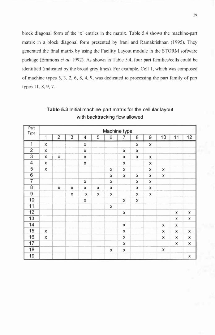
For the cellular layout with backtracking flow allowed, Production Flow Analysis

(Burbidge 1 989) was used for identifying part families and forming cells. First, the

processing requirements of part types on machines were represented by a machine-part

matrix, as shown in Table 5 . 3 . An 'x ' appearing at the intersection of row i and column}

of the machine-part matrix indicates that machine } was required for processing part i.

For example, machine types 1 , 2, 4, 7, 8, 9 were required to process part type 3 . Note

that in the matrix, the machine types required for processing individual part types are

not necessari ly in the order of corresponding operation sequences.

In order to al locate machine types to cells and part types to part fami l ies the order of

the rows and columns of the initial machine-part matrix must be rearranged to find a

29

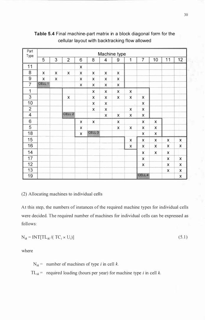
block diagonal form of the 'x ' entries in the matrix. Table 5 .4 shows the machine-part

matrix in a block diagonal form presented by I rani and Ramakrishnan ( 1 995). They

generated the final matrix by using the Facil ity Layout module in the STORM software

package (Emmons et al. 1 992). As shown in Table 5 .4, four part fami lies/cells could be

identified (indicated by the broad grey l ines). For example, Cell 1 , which was composed

of machine types 5, 3 , 2, 6, 8, 4, 9, was dedicated to processing the part family of part

types 1 1 , 8, 9, 7 .

Part Type

Table 5.3 I n it ial machine-part matrix for the cel lu lar layout

with backtracking flow al lowed

Machine type 1 2 3 4 5 6 7 8 9 1 0 1 1 1 2

1 x �_.... .... · I ' I � 1 -L 1--2 --1-'-" +- � j

.... ......

.....

- l -� - :-:--. tr .. �--"-"t- x -� ... � F:�r, .. �--I-----+---I I---!---i .. - .. -� .... J -.?<-- - -- - ..... -. .. �------ .. -- � .. ..... � .. --� - 1 -"-- -" - --I�--i

I---�---. -... I -L __ .. ---.---.. -f---I!---+----I 5 x I x x x X I----+--i__ 6 x x x x x 7 x x x x I 8 X i X x x x x x l t---:--t ...............

................ , ........................... -I .. -.... -............... + . .......... -... ...t ...... -.... · ............ · .. +· .... .... ·.......... + -..... -........... c· .. · ........ ·---.. t ·- .. · .. · .. ·-·· .... · .. ·L-..... -......... ---t-----t

t--_9_, ......... . _ .. __ +i .... _. __ I,_ .... x ... _ ... _ .... ,1 __ ... _x ....... _ ...... I-............ x .... _ ........ + .... _._X._ .. _f ................ _ .. _ ....... il._X_._ .. r ... _ ...... x ......... _ ..... +-I .. _ .............. _ . ... _ .. _ _ _ t--�-�---4 .. --.-... -....... , .. ---.-........ +_ ...... . _ ...... +. _._X_._ .... t ....... -...... -.-... -+I-.-X ........ --i--._X-.... -.. +-.. -X--I ..... -.-.... -.... +-___ __''',_

I------t ........... --j----r---.. I!----+---f---+--t----t---t---j---t----i 1 2 x x x I----j-...... ·· .. ----!---·---·--f----f---+---!---f--- -·---+--f--+----I---I 1 3 x x t--i-i---4 =�-+ ..... -....

.. --+I:· .. -.. · .... · .. --·-

-

.. +-.. --+ .. .. -·-- �· ---+-·· : r -....

. tl--:--t--:"-+-�--i 1 7 ---....

-.-. .. --'-... ---Ir .. -.---.+ ............ --

.... -I--..... -..... X-i� _ _ ...... _ ..... ---I_---I_x---l_x--t 1 8 x x i I x 1 9

.... --r.. -- - ....... --- ..... X-i I

Part Type

Ta ble 5.4 Fina l machine-part matrix in a block d iagonal form for the

cel lu lar layout with backtracking flow al lowed

Machine type 5 3 2 6 8 1 4 9 1 7 1 0 1 1

30

1 2

r-=��--�--�I---; � I x ��.I�x--�

I-�--+--�-+--�---;

.--1_8 __ 1- _ __ ....... _ _ +. _ _ . __ ._._f . __ ._ _

x CELL311 x x 1 5 j x x x x x 11 46 . - . -.i -- -----�.-... ---

..... -.- --t--.--... --.-..

.

.

.

.

....

-...... ---.--

.

.

. --.-

...

.

1-.--. -.-.... _

x--t

: -· --�:=I= X =· .... -x----- --x--x x x I----t-----·---!---+---f----f·-··-.. -.. ---t-·--,f ----f----I---+--+_--t---t

I--j-�-�-:: :-=:--t -1+-=1 =-t -=r-·---i-·+-· ---I-C-�-L-4+----+--:--t-�-i

(2) Allocating machines to individual cel l s

At this step, the numbers of instances of the required machine types for individual cells

were decided. The required number of machines for individual cells can be expressed as

follows:

Nik = INT[TLik I( Tei x Di)]

where

Nik = number of machines of type i in cel l k.

TLik = required loading (hours per year) for machine type i in cell k.

(5 . 1 )

U; = maximum uti l isation rate for machine type i = 0 .9 for all i.

TC; = avai lable annual capacity for each machine of type i

3 1

However, since the lot sizes for individual part types would affect TL;k (Smaller lot

sizes will result in more production lots (batches), and therefore more machine loading

time has to be spent in setting up the machines), it is necessary to incorporate lot sizing

in the allocation of machines. Accordingly, we extended the formula presented by South

( 1 986) so that the order (Kanban) lot sizes for individual part types could be taken into

account in calculating the required machine loading in a cellular layout. In this study, an

order lot size was defined as the number of parts in each batch ( lot) of production (i .e .

for one machine setup). Order lot sizes were the same as the Kanban lot sizes for

individual part types. In other words, the number of parts carried in a standard container

was equal to the order (Kanban) lot size of that specific part type.

Assuming that the shop was operated on two 6-hour shifts per working day with 5

working days per week, the available capacity for each machine would be 3 1 20 hours

for a year of 52 weeks. Therefore, given that the instances of a specific machine type in

a cell are contained in one and only one workstation (Note: This restriction is needed to

avoid the complexity associated with parallel operations when two or more identical

machines are avai lable in a cell for processing a given part.) , the deterministic model of

the required machine loading in each cell can be expressed as fol lows:

p TL;k = I [ INT(D/ Lj) x rjik x TSjik + Dj x TPjik ]

.1= 1

and

c I N;k = N;, for i = 1 , 2, . . . , m

k = 1

(5 .2)

(5 .3)

(5 .4)

where

TLik = required loading (hours per year) for machine type i in cell k.

Dj = demand of part type} (number of parts per year).

Lj = order (Kanban) lot size of part type j. fJik = number of operations required by part type} on machine type i in cell k.

TSjik = setup time for part type} on machine type i in cell k (hours per batch)

TPjik = processing time for part type} on machine type i in cell k (hours per part)

Ui = maximum util isation rate for machine type i = 0.9 for all i. Nik = number of machines of type i in cell k.

32

TCi = available annual capacity for each machine of type i = 3 1 20 hours for all i

p = total number of part types

Ni = total avai lable number of machines of type i c = total number of cells

m = total number of machine types

The lot sizes for the nineteen part types were individual ly adjusted to achieve as high as

possible loading for individual machines, provided the constraints specified by (5 .3) and

(5 .4) were satisfied. At the same time, the loading of individual machines and machine

capacities al located to individual part types in a cell were kept as even as possible. The

final allocation of machines for the cellular layout with backtracking flow allowed is

shown in Table 5 . 5 . Table 5 .6 shows the resulting order lot sizes and annual demands

(in lots) for individual part types.

Note that the annual lot demands derived from the configuration design for both the

cellular and functional layouts were preliminary. To achieve reasonable shop loads, the

prel iminary demands were further fine-tuned by adjusting the mean job inter-arrival

time values for the individual shop configurations. However, the percentages of the total

annual lot demand for individual part types were not changed. The setting of the mean

job inter-arrival time values is described in Subsection 5 . 5 . 1 .

Table 5.5 Allocation of machines for the cel lu lar layout with

backtracking flow al lowed

Cell Al located N umber of Mach ine Type

No. 1 2 3 4 5 6 7 8 9 1 0 1 1 1 2

1 0 1 1 1 1 1 0 1 1 0 0 0

2 1 1 0 2 0 0 1 1 1 0 0 0

3 1 0 0 0 0 2 2 1 1 2 0 0

4 0 0 0 0 0 0 1 0 0 1 2 1

Total 2 2 1 3 1 3 4 3 3 3 2 1

Table 5.6 Order (Kanban) lot sizes and annual lot demands for the cel lu la r

layout with backtracking flow al lowed

Part type Order ( Kanban) Annual demand lot s izes in lots*

1 3 273 2 4 1 86 3 3 295 4 6 2 1 6 5 2 722 6 2 362 7 3 230 8 3 355 9 4 282 1 0 5 1 85 1 1 4 248 1 2 1 6 1 79 1 3 1 0 1 85 1 4 1 9 1 95 1 5 5 1 29 1 6 4 1 62 1 7 1 5 1 48 1 8 2 804 1 9 1 4 57

Total 5,2 1 3 • Based on Dj = 2,500, TSjik = 2 . 1 and TPj ik = 0. 1 .

33

Since backtracking flow was allowed in cells, inter-cell part movement was kept to a

minimum. Only part types 1 5 and 1 6, whose demand accounted for 5 . 1 6% of the total

34

number of parts manufactured annual ly, required inter-cell movement. This was due to

the limitation of the avai lable number of machine type 1 , which was required for

processing part type 1 5 and 1 6. Therefore, part types 1 5 and 1 6 had to be processed on

the machine type 1 in cell 3 , and then moved to cell 4 for the rest of the operations.

(3) Arrangement of the sequences of machines in individual cel ls

The heuristic procedure proposed by Vakharia and Wemmerlov ( 1 990) was uti l ised to

determine the machine sequences in the flow line cel ls by minimising backtracking

flows. The resulting travel charts for the four cells are given in Tables 5 . 7 through 5 . 1 0.

Each row and column of the travel chart represents a machine type that is required for

processing the family of parts assigned to the cel l . The sequences of machines have

been arranged according to the procedure proposed by Vakharia and Wemrnerlov ( 1 990)

so that backtracks in cells were minimised. In addition to the machines required, an

input and output sections were added to each cel l . Each entry, xkl, at row k and column I of the travel chart is defined as:

Xkl = total number of batches (in percentage of total number of batches produced

annual ly) which flow from machine type ' k' to machine type ' /' per year for the part

family manufactured by the cel l . The values of Xkk (i .e . the diagonal entries) are not

defined.

The flow parameter (FP) which is the ratio of the number of backtracks of batches

(weighted by the 'distances' between operations) to the number of forward moves of

batches, was used as a measure of backtracking movements of parts in a cel l .

35

Table 5.7 Travel chart for Cell 1

Unit· % of total batches per year to

from in 3 5 2 6 4 8 9 out

in - 0 . 1 22 0.092 3 - 0. 1 22 5 - 0.068 0.054 2 - 0.068 6 - 0. 1 66 0.048 4 - 0. 1 66 8 - 0 . 1 66 9 - 0. 1 66

out -

FP = 0

Table 5.8 Travel chart for Cell 2

Unit· % of total batches per year

to from in 1 2 4 8 7 9 out

in - 0. 1 86 0.036 1 - 0 .057 0. 1 30 2 - 0.057 4 - 0. 1 24 0. 1 69 8 - 0.036 0. 1 09 0.036 7 0.071 0.057 - 0.041 0.036 9 - 0. 1 50

out -

FP = 0 .31

Table 5.9 Travel chart for Cel l 3 Un it: % of total batches per year

to from in 1 6 1 0 7 8 9 out

in - 0. 1 94 0.224 1 - 0. 1 39 0.056 6 - 0.208 0. 1 54 1 0 - 0.208 0. 1 54 7 0. 1 54 - 0.069 0. 1 39 8 - 0.069 9 - 0.208

out -

FP = 0. 1 4

- - -----------

36

Table 5. 1 0 Travel chart for Cell 4 un it: % of total batches per year

to from in 1 1 7 1 0 1 2 out

in - 0. 1 36 0.056 0 .01 1 1 1 - 0. 1 00 0.056 0 .09 1 7 0.056 - 0.037 0.063 1 0 0.056 - 0.037 1 2 - 0 . 1 65 out -

FP = 0.38

The smaller the FP, the lower was the amount of backtracking movement in a cell . I t

was defined as :

K L K L FP = [ I I x kl ( k - 1 ) ] I[ I I X kl

where:

k = 1 1=1 k=1 1= 1 l<k k --+ I

Xkl = as defined previously.

k � 1 = operation ' k' immediately precedes operation ' l' .

K = L = number of rows (or col umns) in the travel chart.

(5 .5)

The final cel l configurations of the cellular layout with backtracking flow allowed are

summarised in Table 5 . 1 1 . The ' machine sequence' in the table indicates the types of

machines assigned to a cel l , and the sequence in which they were arranged along the U­

shape loop.

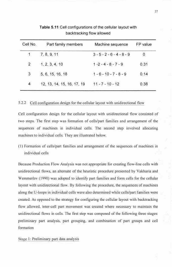
Table 5.1 1 Cell configurations of the cel lu lar layout with

backtracking flow a l lowed

Cell No. Part family members Machine seq uence FP value

1 7 , 8 , 9, 1 1 3 - 5 - 2 - 6 - 4 - 8 - 9 0

2 1 , 2 , 3 , 4 , 1 0 1 -2 - 4 - 8 - 7 - 9 0 .3 1

3 5 , 6 , 1 5 , 1 6 , 1 8 1 - 6 - 1 0 - 7 - 8 - 9 0 . 1 4

4 1 2 , 1 3 , 1 4 , 1 5 , 1 6, 1 7 , 1 9 1 1 - 7 - 1 0 - 1 2 0 .38

5 .2 .2 Cel l configuration design for the cellular layout with unidirectional flow

37

Cell configuration design for the cellular layout with unidirectional flow consisted of

two steps. The first step was formation of cells/part famil ies and arrangement of the

sequences of machines in individual cel ls. The second step involved allocating

machines to individual cells. They are i l lustrated below.

( 1 ) Formation of cells/part families and arrangement of the sequences of machines in

individual cells

Because Production Flow Analysis was not appropriate for creating flow-line cells with

unidirectional flows, an alternate of the heuristic procedure presented by Vakharia and

Wemmerlov ( 1 990) was adopted to identify part famil ies and form cells for the cellular

layout with unidirectional flow. By following the procedure, the sequences of machines

along the U-Ioops in individual cells were also determined while cells/part fami lies were

created. As opposed to the strategy for configuring the cellular layout with backtracking

flow allowed, inter-cell part movement was created where necessary to maintain the

unidirectional flows in cells. The first step was composed of the fol lowing three stages:

preliminary part analysis, part grouping, and combination of part groups and cell

formation

Stage 1 : Preliminary part data analysis

38

At this stage, parts were classified into three mutually exclusive sets as fol lows:

(a) Set <D , consists of part types 1 1 , 1 3 and 1 9 . These are the part types with single or

dual operations.

(b) Set <D2 consists of part types 2, 1 0, 1 5 , 1 6. These part types have backtracking in

their operation sequences.

(c) Set <D3 consists of part types 1 , 3-9, 1 2, 1 4, 1 7 and 1 8 . There is no backtracking in

the sequences of operations for these part types.

Stag� 2 : Part grouping

At the second stage, part groups consisting of the part types in sets <D2 and <D3 with

identical operation sequences, were created. For example, the operation sequences for

part types 1 , 3 and 4 are { l ,4,8,9 } , { 1 ,2,4,7,8,9 } and { 1 ,4,7,9 } , respectively (See Table

5 . 1 ) . S ince both the operation sequences of part types 1 and 4 are contained in that of

part type 3 , the three part types can be merged to form a part group with the composite

operation sequence, { 1 ,2,4,7,8,9 } . Sets <D2 and <D3 were treated separately. Table 5 . 1 2

gives the part groups created and their operation sequences, OR' .

Stage t Combination of part groups and cell formation

Part groups were merged and cel ls were formed in this stage. A similarity matrix, SO

(Vakharia and Wemmerl6v 1 990) was first computed for the part groups without

backtracks (Group p). Then the part groups were merged to form larger groups with

composite operation sequences based on the similarity measures among the part groups.

Final ly parts with single or dual operations and with backtracks (Group g and r) were

allocated to the composite operation sequences and cel ls were formed.

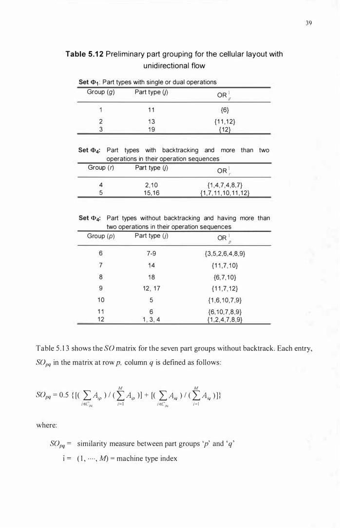
Table 5.1 2 Prel iminary part g rouping for the cel lu lar layout with

un id i rectional flow

Set <l>f Part types with single or dual operations

Group (g) Part type (j) OR I g

2 3

1 1 {6}

1 3 1 9

{ 1 1 , 1 2} { 1 2}

Set <1>4: Part types with backtracking and more than two operations in their operation sequences

Group (r) Part type (j) OR I r

4 5

2 , 1 0 1 5, 1 6

{1 ,4 ,7 ,4 ,8 ,?} { 1 ,7 , 1 1 , 1 0, 1 1 , 1 2}

Set <1>4: Part types without backtracking and having more than two operations in their operation sequences

Group (p) Part type (j) OR I p

6 7-9 {3,5 ,2 ,6,4,8 ,9}

7 1 4 { 1 1 ,7 , 1 0}

8 1 8 {6, 7, 1 0}

9 1 2 , 1 7 { 1 1 ,7 , 1 2}

1 0 5 { 1 ,6 , 1 0 ,7 ,9}

1 1 6 {6, 1 0,7 ,8 ,9} 1 2 1 , 3 , 4 { 1 ,2 ,4 ,7 ,8 ,9}

39

Table 5 . 1 3 shows the SO matrix for the seven part groups without backtrack. Each entry,

SOpq in the matrix at row p, column q is defined as follows :

M M SOpq = 0.5 { [( I A,p ) / ( I A,p )] + [( I A'Q ) / ( I A'Q ) ] } where:

SOpq = similarity measure between part groups 'p' and 'q'

I = ( 1 , . . . . , M) = machine type index

{a

l if machine type I i' is required to process parts in part group I p'

otherwise

Cpq = set of machine types whose members appear in both OR � and OR � in the

same relative order.

Table 5.1 3 SO matrix for the part g roups without backtracks (Group p)

6 7 8 9 1 0 1 1 1 2

6 -7 0 -

8 0 0.67 -

9 0 0.67 0 -

1 0 0 .34 0 0 .53 0 -1 1 0 .51 0 0 .53 0 0.80 -1 2 0.62 0 0 0 0.37 0 .55 -

40

SOpq measures the proportion of machine types used by two part groups 'p' and 'q' in

the same order. The Vakharia and Wemmerlov' s procedure involves an iterative process

of clustering part groups in descending order of their SO measures. However, their

procedure unavoidably may lead to greatly different cell sizes. In addition, since they

allocated all part groups with backtracks to a single cel l , their procedure is not sufficient

for creating pure unidirectional flow l ine cel ls required for this study. Thus instead, a

modified procedure was adopted in this study for cell formation.

First, by examining the SO matrix, we decided that the three clusters of the part groups,

{ 1 O, l l } , { 7,8,9 } and { 6, l 2 } were merged to form three basic composite groups because

of their larger SO measures. The unidirectional composite operation sequences for the

three basic composite part groups are:

OR �,o+ , , ) = { 1 ,6, 1 O,7,8,9 } ,

OR �7+8+9 ) = { 1 1 ,6,7, l a, l 2 } , and

OR �6+ 1 2 ) = { 3 ,5, 1 ,2,6,4,7,8,9 }

4 1

Then the part groups with backtracking, and with single and dual operations were

allocated to the three basic composite part groups. To accommodate the part groups

with single and dual operations, and with backtracking, the operation sequences of the

preliminary parts groups in Table 5 . 1 2 were broken down into sub-sequences where

necessary to achieve unidirectional part flow. Since the way of breaking the operation

sequences of the preliminary part groups would affect the loading of individual

machines, this procedure of breaking operation sequences and the next step, allocating

machines to individual cells were actually performed iteratively to meet the constraint

of avai lable numbers of individual machine types and to achieve as even cell sizes as

possible.

The resulting reorganised part grouping is presented in Table 5 . 1 4. Both part groups 6

and 1 1 were broken down into two groups because both OR �b and OR �Ih could be

contained in other groups. The operation sequences of the part groups with backtracking

were broken down into sub-groups without backtracking. Note that two machines of

type 1 1 were used in the sequence, OR ;b to avoid backtracking. The reorganised part

groups in Table 5 . 1 4 were then merged to form part famil ies and cells.

The final cel l formation and composite part groups are shown in Table 5 . 1 5 . The

operation sequences shown in Table 5 . 1 5 were the arrangement of the sequences of

machines along the U-loops in individual cells.

As shown in Table 5 . 1 5 , five cells (part famil ies) were created for the cel lular layout

with unidirectional flow. Eight part types, whose demand accounted for 26% of the total

number of parts manufactured annually, required inter-cel l movement. S ince no intra­

cell backtracking was allowed, the FP values for all cells were, therefore, zero.

Table 5 . 1 4 Re-organ ised part g rouping for the cel lu lar layout with

un id i rectional flow

Set <1>1 : Part types with single or dual operations

Group (g) Part type (j) OR 2 g

2 3

1 1 {6}

1 3 1 9

{ 1 1 , 1 2} { 1 2}

Set <1>4: Part types with backtracking and more than two operations in their operation sequences

Group (r) Part type (j) OR 2 r

4a 2, 1 0 { 1 ,4 ,7}

4b 2 , 1 0 {4 ,8}

4c 2 {7}

5a 1 5 , 1 6 { 1 , 7} 5b 1 5 , 1 6 { 1 1 , 1 0, 1 1 , 1 2}

Set <1>4: Part types without backtracking and having more than two operations in their operation sequences

Group (p) Part type (j) OR 2 p 6a 7-9 {3,5,2,6}

6b 7-9 {4,8 ,9}

7 1 4 { 1 1 , 7, 1 0}

8 1 8 {6,7 , 1 0}

9 1 2 , 1 7 { 1 1 ,7 , 1 2}

1 0 5 { 1 ,6 , 1 0 ,7 ,9}

1 1 a 6 {6 , 1 0 ,7}

1 1 b 6 {8, 9}

1 2 1 , 3, 4 {1 ,2 ,4 , 7 ,8 ,9}

(2) Allocating machines to individual cells

42

As for the cellular layout with backtracking flow allowed, equations (5 .2), (5 . 3 ) and (5 .4)

were used to determine the order lot sizes for individual part types, and number of

machines required for individual cells. The resulting machine allocation for individual

cel ls is shown in Table 5 . 1 6 . Table 5 . I 7 shows the order lot sizes and annual demand (in

43

lots) for the cel lular layout with unidirectional flow. The final cell configurations are

summarised in Table 5 . 1 8 .

Table 5.1 5 Final cel l formation for the cel lu lar layout with un id i rectional flow

Cell No. Composite part g roup Operation sequence

1 ( 1 +5a + 1 0+1 1 a) {1 ,6 , 1 0 ,7 ,9} 2 (4a+4c+1 1 b+ 1 2) { 1 ,2 .4 ,7 ,8 ,9} 3 (2+3+5b +7+8+9) {1 1 ,6 ,7 , 1 0 , 1 1 , 1 2} 4 6a {3 , 5 ,2 ,6} 5 (4b+6b) {4 ,8 ,9}

Table 5. 1 6 Allocation of mach ines for the cel lu lar layout with u n id i rectional flow

Cel l Allocated N umber of Machine Type

No. 1 2 3 4 5 6 7 8 9 1 0 1 1 1 2 1 1 0 0 0 0 1 1 0 1 1 0 0 2 1 1 0 1 0 0 1 1 1 0 0 0 3 0 0 0 0 0 1 2 0 0 2 2 1 4 0 1 1 0 1 1 0 0 0 0 0 0 5 0 0 0 2 0 0 0 2 1 0 0 0

Total 2 2 1 3 1 3 4 3 3 3 2 1

- ------

Table 5. 1 7 Order (Kanban) lot s izes and annual lot demands for the cel lu lar

layout with un id i rectional flow

Part type Order (Kanban) Annual demand lot s izes

1 3 2 5 3 3 4 7 5 3 6 2 7 3 8 3 9 2 1 0 6 1 1 4 1 2 1 6 1 3 1 0 1 4 1 9 1 5 5 1 6 4 1 7 1 5 1 8 2 1 9 1 4

Total • Based on Dj - 2,500, TSjik - 2 . 1 and TPjik - 0. 1 .

i n lots*

273 1 49 295 1 85 481 362 230 355 564 1 55 248 1 79 1 85 1 95 1 29 1 62 1 48 804 57

5, 1 56

Table 5.1 8 Cell configurations of the cel lu lar layout with

un id i rectional flow

44

Cell No . Part family members Machine seq uence FP value

1 5 , 6 , 1 1 , 1 5 , 1 6 1 - 6 - 1 0 - 7 - 9 0

2 1 , 2 , 3 , 4 , 6 , 1 0 1 - 2 - 4 - 7 - 8 - 9 0

3 1 2 , 1 3 , 14 , 1 5, 1 6 , 1 7 , 1 8 , 1 9 1 1 - 6 - 7 - 1 0 - 1 1 - 1 2 0

4 7 , 8 , 9 3 - 5 - 2 - 6 0

5 2 , 7, 8, 9, 1 0 4 - 8 - 9 0

5.3 Configuration Design for the Functional Layout

45

When the shop was configured in a functional layout, it was equivalent to there being

only a single cell in the shop. All machines of the same type were allocated in a

functional department. Therefore the functional departments of the functional layout

were regarded as large workstations grouped in a cel l . The only task required for

configuring the functional layout was to determine the order lot sizes for individual part

types so that the constraint of avai lable machine capacity was satisfied. As for the

cellular layouts, equations (5 .2), (5 .3 ) and (5 .4) were used to determine the appropriate

order lot sizes. The order lot sizes and annual demand (in lots) for the functional layout

is given in Table 5 . 1 9 .

Table 5.1 9 Order (Kanban) lot sizes and annual lot demands for the

functional layout

Part type Order (Kanban) lot sizes

3 2 4 3 2 4 6 5 3 6 2 7 3 8 3 9 3 1 0 5 1 1 3 1 2 2 1 1 3 1 2 1 4 9 1 5 4 1 6 3 1 7 1 7 1 8 2 1 9 1 2

Total

Annual demand in lots*

395 270 640 31 3 698 524 333 5 1 5 545 269 479 1 98 223 597 234 3 1 2 1 89

1 1 66 96

7 ,996 • Based on Dj - 36,250, TSj ik - 0.97 and TPj ik = 0. 1 .

5.4 Design of the Shop Layout

46

The purpose of the shop layout design process was to position the departments / cells in

the avai lable shop floor area to achieve as few inter-department/cell part movements as

possible. As i l lustrated in Chapter 4, one of the research questions to be answered

through this research project was whether different shop layouts (functional layout and

various cel lular layouts) made any difference in the performance of job shop

manufacturing with Kanbans. To correctly investigate the influence of shop layout, it

was essential that the relative positions among departments / cel ls were carefully

designed because different relative positions would lead to different part movement

distance and in turn, different shop performance.

In the shop modelled, each machine (including the input and output buffers, and

auxil iary faci l ities) had a footprint of 1 4 feet by 1 4 feet. The total avai lable shop floor

area was 84 feet by 84 feet. In addition to functional departments / manufacturing cells,

a receiving and a shipping departments were added to all layouts. All jobs were initiated

in the receiving department and terminated in the shipping department. The methods of

Systematic Layout Planning (Muther 1 973) were employed to allocate the functional

departments / manufacturing cells to the available shop floor area. The procedure of

Systematic Layout Planning involved three steps. At the first step, Flow relationship

diagrams, which were based on the intensity of flows among cells / departments, were

constructed to determine the importance of closeness among cel ls / departments. At the

next step, space relationship diagrams were prepared by individually placing the areas

of cells / departments in the shop floor area according to the information provided by

the flow relationship diagrams. Finally, the resulting space relationship diagrams were

then used to determine the travel li ng distances of part movement among workstations as

well as among cells / departments. The three steps of the shop layout design are

individually i l lustrated below.

5 .4 . 1 Preparation of the flow relationship diagrams

47

To construct the flow relationship diagrams for the three basic shop layouts ( i .e. the

cellular layout with unidirectional flow, the cel lular layout with backtracking flow

allowed and the functional layout), the ' from-to charts' for the various shop layouts had

to be prepared first. Table 5 .20 shows the from-to chart for the cellular layout with

unidirectional flow. Each entry xi}, at row i and column } of the from-to chart indicates

the total number of batches of parts which flow from cell / department i to cell /

department } per year. For example, as shown in Table 5 .20, there were 3 04 batches of

parts flowing from cell 2 to cell 5 annual ly. The from-to charts for all the three basic

layouts are given in Appendix 1 .

Table 5.20 From-to chart for the cel lu lar layout with un id i rectional flow

un it : batches per year From To (Cell) (Cell)

I n 1 2 3 4 5 Out

* 1 382 1 057 1 568 1 1 49 I n --

1 -- 362 291 729

2 -- 304 1 264

3 -- 1 859

4 -- 1 1 49

5 149 -- 1 304

Out* --. . * " I n" represents the receiving department, and "Out" , the shipping department.

Next, from the from-to charts, the total annual number of batches travelling between

each pair of cells / departments in both directions ( i .e . flow-of-material intensity) was

calculated for each shop layout. The flow-of-material intensity values for each shop

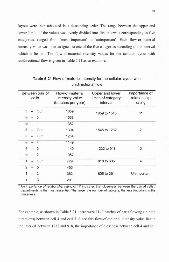
48

layout were then tabulated in a descending order. The range between the upper and

lower l imits of the values was evenly divided into five intervals corresponding to five

categories, ranged from 'most important' to 'unimportant' . Each flow-or-material

intensity value was then assigned to one of the five categories according to the interval

which it l ies in . The flow-of-material intensity values for the cellular layout with

unidirectional flow is given in Table 5 .2 1 as an example.

Table 5.21 Flow-of-material i ntensity for the cel lu lar layout with

un id i rectional flow

Between pair of Flow-of-material Upper and lower Importance of cel ls i ntensity value l im its of category relationship

(batches per year) i nterval rating

3 Out 1 859 1 859 to 1 545 1 * I n 3 1 568 I n 1 1 382 5 Out 1 304 1 545 to 1 232 2 2 Out 1 264 I n -- 4 1 1 49 4 5 1 1 49 1 232 to 9 1 8 3 I n 2 1 057 1 Out 729 91 8 to 605 4 2 5 453 1 2 362 605 to 291 Unimportant 1 3 291

* An importance of relationship rating of ' 1 ' ind icates that closeness between the pair of cells / departments is the most essential. The larger the number of rating is, the less important is the closeness.

For example, as shown in Table 5 .2 1 , there were 1 1 49 batches of parts flowing (in both

directions) between cell 4 and cel l 5 . Since this flow-of-material intensity value l ies in

the interval between 1 232 and 9 1 8, the importance of closeness between cell 4 and cell

49

5 was classified as ' 3 ' .The flow-of-material intensities for the three basic shop layouts

are l isted in Appendix 2 .

The importance of relationship ratings for the three basic shop layouts were then

presented in the form of flow relationship diagrams. As an example, F igure 5 . 1 shows

the resulting flow relationship diagram for the cellular layout with unidirectional flow.

0::::::::::::- · ·- · 0 : : _ . . - . : :::: : : :::: : : :::: : : :::: : : 5 I : t , I I I

' "

I I I I I I

I

I I I I

.4Ai<' , (�) }�

� ' ',> . . . . . . . . . '

,� LEGEND

ri"� . . . .. �:. � "

U ····· · · · · · · · · · · · · · · · � �� · ? W Receiving department

W S hipping department

o Manufacturing cell

Importance of relationship

1 = = = 2 = : : = : : = 3 . . . . . . . . . . . . . 4 No connection: unimportant

Figure 5.1 Flow relat ionship d iagram for the cel lu lar layout with

un id i rectional flow

By presenting the relationship between cells / departments in graphic symbols, the

importance of closeness between each pair of cells / departments was more easily

recognised visually through the flow relationship diagrams. The flow relationship

diagrams for al l the three basic shop layouts were presented in Appendix 3 . These

50

resulting flow relationship diagrams constituted the basis for preparmg the space

relationship diagrams in the following subsection.

5 .4 .2 Preparation of the space relationship diagrams

The space relationship diagram shows the exact relative positions among cells /

departments in the avai lable shop floor area. The space relationship diagrams were

constructed by inserting the 'blocks' representing the required areas for cells/

departments into the available shop floor area. The blocks for cells / departments were

inserted one pair at a time, beginning from the pair with the highest importance of

closeness ( i .e. the pair(s) with importance of relationship rating of ' 1 ' ) through the ones

with ' unimportant' ratings. In the process of inserting blocks, the orientation and

relative positions of inserted blocks were adjusted when necessary to fit into the

confines of the available shop floor area.

As an example, the space relationship diagram for the cel lular layout with unidirectional

flow is presented in Figure 5 .2 . From Figure 5 . 1 , we knew that the closeness between

cell 3 and the receiving department, and between cell 3 and the shipping department was

the most important. Therefore, the area blocks for cel l 3 , the receiving department and

the shipping department were inserted in the shop floor area first. Note that the

receiving and the shipping departments were both placed next to cell 3 to shorten the

travel l ing distances of parts between the two departments and cell 3 .

After positioning the cells / departments with the most important relationships, we then

looked at the relationships with next importance ratings ( i .e . the rating '2 ' ) . From Figure

5 . 1 , we knew that the importance of the relationships for the three pairs, cell 1 -

receiving department, cell 2 - shipping department and cell 5 - shipping department was

rated '2 ' . Therefore, the block for cell 1 was inserted next to the receiving department.

Then the blocks for cell 2 and cel l 5 were positioned next to the shipping department.

5 1

Final ly, cell 4 was placed at a position as close to the receiving department and cel l 5 as

possible, since the importance of the relationships between cell 4 and the receiving

department, and between cell 4 and cell 5 was rated ' 3 ' . However, the closeness of cell 4

to the receiving department and cell 5 was not as essential as that of previously

considered relationships.

CELL 1

I Q- - , 1 I 1

7 1 1

CELL 4 6 m � - -> []

1 (OUT)

3 (IN)

84' 0"

CELL 3

-l 0 1

� O 8... 1

Shipping Dept.

Cl tTl r r Vl

CELL 2

, 7

b 't co

LEGEND

__ I nter-cell part movement path

Intra-cell part - -> movement path

with conveyors

� Cell incoming job storage

EEl Cell outgoing job storage

D Machine footprin ( 1 4 Ft x 14 ft)

Figure 5.2 Space relationship d iagram for the cel lu lar layout with

un id i rectional flow

By fol lowing the procedure, pairs of cells I departments with more important

relationship ratings were placed closer to each other and eventually, a reasonably

arranged shop layout could be obtained. Possible alternative orientations and positions

of cel ls were also considered in the procedure to achieve better results. The same

procedure was fol lowed to prepare the space relationship diagrams for other layouts.

The completed space relationship diagrams for the three basic shop layouts were given

in Appendix 4.

--------

5 .4 .3 Determination of the inter-cell / department and intra-cell travell ing distances.

52

After the space relationship diagrams were created, the travel l ing distances of parts

between workstations / cells / departments could then be obtained by directly measuring

these distances on the diagrams. The travell ing distance between two workstations was

measured between their centre points. In this study, we also took into account the

possibi l ity that different material handl ing methods could lead to different intra-cell

travel ling distances.

We wil l take cell 1 in Figure 5 .2 as an example. If parts are moved from machine type 1

to machine type 9 by a worker, who can move directly between the centre points of the

machines, the travell ing distance is 1 4 feet. However, if parts are moved by a conveyor

in the cell, parts at machine type 1 have to travel along the U-Ioop (i .e . through machine

types 6, 1 0, 7) before reaching machine type 9. The travel ling distance in this case will

be 70 feet. Therefore, for each cel l , the intra-cel l distance matrices for both manual

material handling and material handling by a conveyor were constructed.

As an example, Table 5 .22 gives the intra-cell travel l ing distance matrix with material

handling by a conveyor for cell 1 of the cellular layout with unidirectional flow. The

intra-cell travell ing distance matrix for the same cell, but with manual material handling

is presented in Table 5 .23 . The differences in the intra-cel l travel l ing distances because

of the different material handl ing methods can be distinguished between the two

matrices. The complete intra-cel l travel l ing distances matrices are given in Tables A5 . 1

through AS . 1 8 i n Appendix 5 .

The travel ling distance between two cel ls / departments was measured from the

outgoing storage of the preceding cell / department to the incoming storage of the

succeeding cel l / department. Inter-cell / department distance matrices for the three basic

shop layouts are given in Tables A5. 1 9 through A5.2 1 in Appendix 5. The travel l ing

distance matrices were later incorporated in the simulation model of the shop

53

environment, and used for calculating travel l ing times of part movements during

simulation runs.

Table 5.22 I ntra-cel l d istance matrix for Cell 1 with un id i rectional flow

(material handl ing by a conveyor)

un it : feet

From To Workstation No.lMachine Type Workstation No.!

Machine type I n 1 /1 2/6 3/1 0 4/7 5/9 Out

I n -- 7 2 1 49 63 77 84 1 /1 -- 1 4 42 56 70 77

-- --

2/6 -- 28 42 56 63 --

3/1 0 -- 1 4 28 35 ---

4/7 -- 1 4 2 1 ---------

5/9 -- 7 . . _----------- ---

Out --

Table 5.23 I ntra-cel l d istance matrix for Cell 1 with un id i rectional flow

(manual material handl ing)

u nit: feet

From To Workstation No.lMachi ne Type Workstation No.!

Machine type I n 1 /1 2/6 3/1 0 4/7 5/9 Out

I n --

__ Jj5 49 35 2 1 --

1 /1 -- 28 42 28 1 4 2 1 --- ----

2/6 -- 28 1 4 28 35 ._--- ------------f--

3/1 0 -- 28 42 49 ---_._.- _ ... _--

4/7 -- 28 35 --- -

5/9 I -- 7 ------_ .. _ .. _ . .

i Out 1 --

5.5 Design of the Shop Operations

In the shop model, the shop operations included the fol lowing four elements:

arrival of jobs: introducing new jobs i nto the system,

production control : routing jobs through the shop,

processing of jobs, and

material handl ing speed settings.

54

For the design of the shop operations, we defined the algorithms and parameters

regarding the four elements. The design of the four elements are described in detail in

the following subsections.

5 . 5 . 1 Arrival of jobs

To simulate the irregular demand pattern of a job shop environment, the inter-arrival

times of jobs were assumed to be exponentially distributed. I n order to have a fair

comparison of the shop performance across difference shop configurations and

parameters, the mean values of job inter-arrival time were manipulated so that the same

amount of each part type was manufactured annually for al l the three basic shop layouts

( i .e . functional layout, cellular layout with unidirectional flow and cellular layout with

backtracking flow allowed). The mean job inter-arrival time for a specific basic layout

was calculated as the total working hours per year divided by the total number of lots

produced per year:

p TMJI = WH / I INT(Dj / Lj) (5 .6)

.1=1

where

TMJI = mean job inter-arrival time

WH = working hours per year = 3 1 20 hours

Dj = demand of part type} (number of parts per year).

Lj = order (Kanban) lot size of part type j. p = total number of part types = 1 9

55

As mentioned above, Dj was the same for al l the three basic layouts. S ince Lj, } = 1 , 2,

. . . , p, were different for the three basic layouts, one mean job inter-arrival time value

was needed for each basic layout. In addition, the job inter-arrival time for a specific

basic layout was also affected by the part family setup reduction factor (PFSRF) used in

this study (See Subsection 5 .5 .3 ) . The PFSRF represents the portion of the standard

setup time required when consecutive jobs processed on a machine belong to the same

part fami ly . As the part fami ly setup reduction factor became smaller, the machine

loading was lower because less time was spent for setting up machines. Consequently,

more parts can be produced by the shop at lower PFSRFs (i .e. Dj was larger at lower

PFSRFs). S ince three PFSRF levels, 0.7, 0 .5 and 0.2 were used in this study (See

Section 6. 1 . ), a set of job inter-arrival time values was needed for each level of the

PFSRF.

To obtain the suitable mean job inter-arrival time values, preliminary simulation runs

were performed for the cellular layout with backtracking flow allowed and single unit

production & conveyance, at each of the three part family setup reduction factor levels,

to find out the annual demand level, Dj at which the average bottleneck machine

uti l isation reached about 66%. One set of Dj was therefore obtained for each level of

PFSRF. The three sets of Dj for the three PFSRF levels were then used in equation (5 .6)

to calculate the mean job inter-arrival time values for the three basic layouts. The mean

job inter-arrival time values are summarised in Table 5 .24. I n total, nine mean job inter­

arrival t ime values (3 basic layouts at three levels of part fami ly setup reduction factor)

were used.

Upon the arrival of a job, the probabi l ity of a specific part type being assigned to the job

is given in Table 5 .25 . The probability value for a part type was obtained by calculating

the percentage of total batches of parts produced for that part type.

56

Table 5.24 List of mean job inter-arrival t ime values

Level of Shop layout Mean job inter- Average annual total number of

PFSRF arrival time (hrs) parts manufactured (pcs)

Functional layout 0 .7069 20000 0 .7 CLUF* 0.7564 20000

CLBF** 0.7481 20000 Functional layout 0 .5953 23750

0 .5 CLUF 0.6370 23750 CLBF 0 .6300 23750

Functional layout 0 .3900 36250 0.2 CLUF 0 .4 1 73 36250

CLBF 0 .4 1 28 36250 * Cellular layout with unidirectional flow * * Cellular layout with backtracking flow al lowed

For example, as shown in Table 5 .6 of Subsection 5 .2 . 1 , through the process of

allocating machines to individual cells for the cellular layout with backtracking flow

allowed, we arrived at the total number of batches ( lots) of parts manufactured per year

was 52 1 3 . I n addition, among these annual total batches manufactured, the total number

of batches manufactured for part type 1 was 273 . Accordingly, the probability value for

part type 1 for the cellular layout with backtracking flow allowed was 273/52 1 3 =

0.0524 or 5 .24%, as shown in Table 5 .25 . In other words, in the long run, 5 .24% out of

the total batches of parts produced by the shop belonged to part type 1 .

Once the part type for an arriving job was decided, the lot size for the part type (as given

in Table 5 .6, 5 . 1 7 or 5 . 1 9, according to the basic shop layout investigated) was assigned

to the job, and a container of parts with the specified part type and lot size was then

launched into the system.

--- ------------

Table 5.25 Probabi l ity of part types to be assigned to an arriving job

Part type Functional Cellular layout with Cellular Layout with layout unidirectional flow backtracking flow allowed 0.0494 0.0529 0.0524

2 0.0338 0.0289 0.0357

3 0.0800 0.0572 0.0566

4 0.0391 0.0359 0.04 1 4

5 0.0873 0.0933 0. 1 385

6 0.0655 0.0702 0.0694

7 0.04 1 6 0.0446 0.0441

8 0.0644 0.0689 0.0681

9 0. 0682 0. 1 094 0.0541

1 0 0.0336 0.030 1 0.0355

1 1 0 .0599 0.0481 0.0476

1 2 0.0248 0.0347 0.0343

1 3 0.0279 0.0359 0.0355

1 4 0.0747 0.0378 0.0374

1 5 0.0293 0.0250 0.0247

1 6 0.0390 0.03 1 4 0.03 1 1

1 7 0 . 0236 0.0287 0.0284

1 8 0 . 1 459 0 . 1 559 0. 1 543

1 9 0 .01 20 0 .01 1 1 0 .01 09

5 .5 .2 Production control using a hybrid push/pull Kanban system

57

To apply the Kanban-based production control method to the job shop environment, a

hybrid push/pull Kanban system instead of a 'pure' Kanban system was adopted in this

study. The pure demand-pull Kanban system is the typical Kanban system used for

repetitive manufacturing environments, where demand (both in volume and product

types) is much more stable than that of job shop environments. Smooth operation of

such Kanban system, where component replenishment is triggered by the demand at the

final assembly l ine requires that:

58

( 1 ) Fixed and l imited stock of parts is kept at each stage for the consumption by the

succeeding stage, and

(2) Signals are issued for replenishment of parts to be stocked at each stage when

necessary.

However, these requirements are not l ikely to be attainable in the job shop environment.

Since job shop environments are usually characterised by i rregular demand patterns (in

volume and/or product mixes), it is not cost-effective to keep a fixed stock of all the part

types manufactured. Besides, without a uniformly sequenced final assembly schedule,

there is no consumption of parts at the next higher assembly level to signal the need for

replenishment (Kelleher 1 986, Stockton and Lindley 1 995).

Therefore, to adapt the Kanban-based production control method to the job shop

environment, a hybrid push/pul l Kanban system (Gravel and Price 1 988, Lee et al. 1 994,

Li and Nahavandi 1 997) was used instead for production control .

As shown in Figure 5 .3 , in the hybrid system, each cell (department) was assigned an

incoming storage area for keeping containers carrying materials or parts to be processed

and an outgoing storage area where containers holding processed parts to be transported

to other cel ls (departments) were stocked. A specific number of empty

container/conveyance Kanban sets (denoted by CD and <ID) were allocated in the outgoing

storage area for each part type produced in a cell (department).

Empty containers served as production Kanbans as wel l as storage spaces for holding

processed parts. Each container was associated with a conveyance Kanban that

authorises the moving of the container to the succeeding cell (department) designated by

the Kanban. When a job order was released to the shop, the required materials or parts

were launched to the incoming storage area of the first cel l (department) on its routing.

However, the job could only be processed when there was an available empty container

(production Kanban) (denoted by @) for storing the processed parts. Processed parts

59

were stored in a container (denoted by ®) and kept in the outgoing storage until an

available conveyance Kanban (denoted by ®) authorising the movement of the specific

container was present. The conveyance Kanban was then attached to the container

(denoted by ®), which was transported to the incoming storage area of the succeeding

cell (department) specified by the Kanban.

from prec eding

C

Cell A Incoming storage

Cell A Outgoing storage

....... Cell B

Incoming storage .. . . @] ill

Cell B Outgoing storage from

succeeding cell

� __ lcCK I D <D &J B CK � ..... .,. I@JD B �. ··· IT � " ' ....

. ....... ."

to P

I@D I1 , \ �J� �\

" . ·· ·�JcCK ID receding

\ cell

.. . ,. .. @

\ 6 � � @ ',--

Workstation area Cell A

LEGEND ,...." filled fCK1 conveyance LY container � Kanban

� empty -----+ container LY container flow

V

\ � 2=v Workstation area

Cell B

.......... • Kanban flow

@] -.. \ ' \ t

@] ....

to s ucceeding cell

Figure 5.3 Operation of the hybrid push/pul l Kanban system among cells

When parts in a container at the incoming storage began to be processed, the attached

conveyance Kanban (denoted by CD) was removed and sent back to the preceding cell

(department). A container was sent back to the outgoing storage of the preceding cell

(department) when emptied (denoted by @). The procedure was thus continued until the

job was completed. In such a system, instead of being triggered by the requirement at

the final assembly l ine, the production process was initiated by 'pushing' materials or

60

parts into the system, and then parts were 'pul led' through cells (departments) according

to Kanban signals.

The operation of the hybrid push/pull Kanban system among workstations within a cell

is presented in F igure 5.4. The incoming and outgoing storage areas of cells are now

replaced by the input and output buffer of workstations, respectively. Containers and

Kanbans were circulated among workstations in the same manner as that among cells.

The functional departments of the functional layout were regarded as workstations in a

single cel l .

om fr prec

work eding station

Workstation A Workstation A Input buffer Output buffer

(!) � �lccK ID CD � B CK . .... .... ........ .... ..

receding to P wo rkstation

".

ICCK ID ;.

'. ..... . 1 �0 1.\ .... @] \ \ � b

.� Process area Workstation A

LEGEND ....-rJ fi l led t'CKl conveyance LY container � Kanban

11==71 empty __ container LY container flow

Workstation B Input buffer

I@D ;;ICcK ID

� ------

Workstation B Output buffer

B �. /

.

I1 �\ \ 2=D

Process area Workstation B

... Kanban flow

. .... \ ....

from succeeding WQ(kstation

'. '.

to s ucceeding WQ(k$tation

Figure 5.4 Operation of the hybrid push/pul l Kanban system among

workstations

6 1

5 .5 . 3 Processing of jobs

Once a job (representing a container filled with parts of a specific part type) was

launched into the shop, it would be routed through and processed at various cells I departments and workstations according to its operation sequence. I n our shop model,

two aspects were related to the processing of jobs: the setup and processing times for

processing parts, and the scheduling of jobs.

(a) Setup and processing times for processing parts

As defined in Section 1 .2, the time required to accomplish the work for processing a

batch of parts on a machine at a workstation comprises two components: the setup time

and the processing time.

Operations on all machines required the same mean processing time of 0 . 1 hours per

part and the actual processing time values of individual operations were derived from

the gamma distribution with a shape parameter, a = 3 . The gamma distribution was

chosen because the histogram of service time data often has a shape similar to that of its

density function (Law and Kelton 1 99 1 ) .

Sequence-dependent setup times were employed in this study. If a job to be processed

on a machine was not in the same part family as the preceding completed job, a ful l

setup would be required. I f two consecutive jobs were of the same part fami ly but

different part types, only a partial setup was incurred. I f the succeeding job was of

exactly the same part type as that of the preceding job, no setup was required at all .

For each setup operation, a major setup time value was generated from the gamma

distribution with an a value of 2 and a mean of 2 hours. The major setup time was then

mUltiplied by a part family setup reduction factor (PFSRF) to obtain the partial setup

time if applicable. Therefore, the lower the PFSRF, the larger is the amount of setup

time reduction achieved by adopting cel lular manufacturing. The a value of 2 was used

because setup times are usually more variable than processing times in a job shop

62

environment. Consequently, in a cel lular layout, the setup times incurred were either

partial or zero since only the same fami ly of parts were processed in a cel l , while in a

functional layout, setup times could be ful l , partial or zero.

(b) Scheduling of jobs

As depicted in Subsection 5 . 5 .2, the hybrid push / pull Kanban system was adopted for

the production control in the shop model . When a job (i .e . a container fil led with parts)

arrived at the incoming storage area of a cell and there was an available empty container

( i .e . production Kanban) for storing the completed parts at the outgoing storage area,

parts in the container would be moved to the input buffer of the first workstation on

their routing if storage space was avai lable. Parts were moved in lots for batch

production and conveyance, and one piece by one piece for single-unit production and

conveyance. I f either an empty container at the outgoing storage area of the cell or

storage space in the input buffer (signified by a conveyance Kanban) of the workstation

was not avai lable, the job would be queued in the incoming storage area unti l both were

available.

After a job was transferred to the input buffer of a workstation, it could only be

processed when there were both an avai lable empty container ( i .e. production Kanban)

for keeping processed parts in the output buffer and an available machine, or it would be

queued in the input buffer unti l both were avai lable. If more than one machines were

available for processing a job, the one having the most similar setup to that required for

the job would be selected. I f al l machines had the same setup, the machine to process

the part was selected at random. When any machine in a workstation became idle, both

a queue selection heuristic and a job selection rule were executed to select a job from

those queued in the input buffer. The queue selection heuristic based on the 'repetitive

lots' procedure (Flynn 1 987) was performed first to search for a job of the same part

type as that of the last processed job. If any one was found, the first one by order of

arrival was selected. This procedure took advantage of sequence-dependent setup times

and attempted to further minimise setups by not switching to another part type until all

63

jobs of the same part type were completed. I f no such matched part type was found, a

job was selected for processing based on the shortest processing time (SPT) job

selection rule. In circumstances when the SPT rule was not able to break ties among

jobs, the first-come-first-serve (FCFS) rule was appl ied to break the ties. As depicted in

the last section, transferring of jobs among workstations was authorised by the

conveyance Kanban signals.

The functional departments of the functional layout operated in the same way as that of

the workstations of a cellular layout as if there had been only one cell in the shop.

However, since jobs processed by a department could be of different part families, the

execution of the queue selection heuristic was a l ittle different. I f a job of the same part

type could not be located, searching for a job of the same part fami ly as that of the last

completed job would be attempted. If sti l l no matched job was found, the procedure was

then reverted to the shortest processing time job selection rule. In this manner, the

benefit of setup time reduction brought about by cellular manufacturing could stil l be

realised indirectly in the functional layout by the adoption of the queue selection

heuristic without physically grouping machines into cel ls.

5 . 5 .4 Material handling speed settings

S ince material handling speed had been claimed to be one of the essential factors for

real ising the benefits of cellular manufacturing (Monden 1 983 : 74, Shingo 1 989: 37),

both inter-cel l (department) and intra-cell material handling speeds were explicitly

incorporated in the shop model to examine their effects on the shop performance. The

settings of material handling speed were derived from the data given by Apple ( 1 963)

and Apple ( 1 972). Both high and low settings were investigated for al l speeds.

Considering the times for loading and unloading parts (stored in containers) with

different sizes and weights may vary significantly, the loading and unloading times were

uniformly distributed.

64

The material handling speed settings for inter-cell I department part movement are

summarised in Table 5 .26. Parts were transported in batches (lots) for inter-cell /

department movement. The high speed setting was based on that of a fork l ift truck. The

travelling speed was 4 miles per hour (mph). Loading and unloading times were

uniformly distributed between 1 0 and 1 4 minutes per batch ( lot) moved. At the low

speed setting, four-wheel hand trucks were used. The travelling speed was 0 .8 mph, one

fifth of the high setting value. Distribution of loading and unloading times was the same

as that for fork l ift trucks.

Table 5 .27 gives the material handling speed settings for intra-cel l part movement with

batch production and conveyance. Parts were transferred among workstations within a

cell in lots with batch production and conveyance. At the high speed setting, l ive rol ler

conveyors with a speed of 6 mph were used. The times for loading and unloading were

uniformly distributed between 0.8 and 1 .2 minutes per batch ( lot) moved. Two-wheel

hand trucks were used at the low speed setting. Their travel l ing speed was 1 .2 mph, one

fifth of the high setting value. Loading and unloading times had a uniform distribution

between 2.4 and 3 .6 minutes per batch ( lot) of parts moved.

Table 5.26 Materia l hand l ing speed sett ings for inter-cel l / department

part movement

Materia l handl ing speed sett ings

High

Low

Equipment type

Fork l ift truck

Four-wheel hand truck

Travel l ing speed

4 mph, constant

0 . 8 mph, constant

Load ing & un load ing time

Uniformly d istributed with Upper l imit: 1 4 min/lot Lower l imit: 1 0 minllot

Un iformly d istributed with Upper l imit: 1 4 min/lot Lower l imit: 1 0 min/lot

For intra-cell part movement with single-unit production and conveyance, parts were

transferred among workstations within a cell one piece by one piece. As shown in Table

65

5 .28, the high setting was the same as that for batch production and conveyance. At the

low speed setting, parts were handled manual ly by workers with a travel l ing speed of

1 .2 mph. Times for loading and unloading were uniformly distributed between 1 4 and

22 seconds per part moved.

Table 5.27 Material handl ing speed sett ings for intra-cel l part movement with

batch prod uction and conveyance

Material handl ing Equipment Travel l ing Load ing & unload ing speed sett ings type speed time

High Live rol ler 6 mph, Uniformly d istributed with

conveyor constant Upper l imit: 1 .2 minllot Lower l imit: 0 .8 minllot

Low Two-wheel 1 .2 mph, Uniformly d istributed with

hand truck constant Upper l imit: 3 .6 minllot Lower l imit: 2.4 minllot

Table 5.28 Material handl ing speed settings for intra-cel l part movement with

s ing le-un it production and conveyance

Materia l handl ing Equipment Travel l ing Load ing & un load ing speed settings type speed time

H igh Live rol ler 6 mph, Uniformly distributed with

conveyor constant Upper l imit: 1 .2 min/part Lower l imit: 0 .8 min/part

Low Manual 1 .2 mph, Uniformly d istributed with

handl ing by constant Upper l imit: 22 sec/part

workers Lower l imit: 14 sec/part

To take into account the adverse effects of backtracking part movement on material

handl ing, it was assumed that intra-cel l backtracking part movement speeds were always

kept at the corresponding low settings. For example, in the case of intra-cel l part

movement with single-unit production and conveyance, backtracking parts were always

handled manually by workers, even when live rol ler conveyors were being used.

66

Besides, as described in Subsection 5 .4 .3 , the fact that different material handl ing

methods may lead to, not only different material handling speeds, but also quite

different travel ling distances was also taken into account in this study. In a

manufacturing cell where a l ive rol ler conveyor was used, parts always had to travel

along the V-loop path from a workstation to another even though the two workstations

are opposite to each others. However, in the case where parts were transported manually

in a cel l , workers were free to move in the area of the cel l and hence always had the

flexibi lity to fol low the shortest path to travel around workstations without being

l imited to a fixed path. Consequently, the two different transportation methods would

lead to different travel l ing distances.

Through the design of the experimental system, we had developed a manufacturing

environment with the necessary features and parameters for our investigation. The

hybrid push / pull Kanban system constituted the fundamental mechanism of the shop

operation since the objective of our study was to investigate the performance of job

shop manufacturing with Kanban-based production control . The resultant algorithms

and parameters through the design stage were later implemented in the simulation

model of the manufacturing shop. The actual performance measures used to evaluate the

shop performance are addressed in Chapter 6.

67

CHAPTER 6

DESIGN OF THE FIRST SET OF EXPERIMENTS

Two groups of simulation experiments were performed in this study. In the first set of

experiments, the influence of four factors: shop layout, production flow patterns,

material handling speed and part family setup reduction factor (PFSRF) on the

performance of job shop manufacturing with Kanbans was investigated.

In the first set of experiments the coefficients of variation (the ratios of standard

deviation to mean) of setup and processing times were held constant for all shop models.

However, as reported by Philipoom et al. ( 1 987), the variability of processing times had

a substantial effect on the performance of a job shop with Kanban-based production

control . Vi l leda et al. ( 1 988) also addressed the influence of the variability of operation

times on a Kanban-based system. Therefore, the second set of simulation experiments

was designed to investigate the influence of the variabil ity (expressed in coefficients of

variation) of processing and setup times on the performance of a job shop environment

with Kanban-based production control .

In the second set of experiments, the coefficients of variation of setup and processing

times were introduced as a factor to investigate their influence on the shop performance.

The material handling speed was treated as a background variable (See Section 9.4 for

detai ls) in this set of experiments and the information gained in the first set of

experiments was uti l ised to determine the material handl ing speed settings. Other

factors investigated were the same as for the first set of experiments. This chapter

covers the design of the first set of experiments. The design of the second set of

experiments is i l lustrated in Chapter 9.

Since this research project was a simulation experiment In nature, a Design of

Experiment approach was essential to plan the way the experiment was conducted and

how the output of the experiment was analysed. The design of the experiment involved

68

the selection of three elements: the independent variables and their levels to be

investigated, the dependent variables to be measured, and the appropriate statistical

analyses of the simulation output.

Note that the definition of independent and dependent variables is taken from Moen et

al. ( 1 99 1 ). A dependent variable is a variable observed or measured in an experiment

( i .e. the outcome of an experiment). An independent variable is a variable that is

deliberately varied or changed in a control led manner in an experiment to observe its

impact on the response variable. The three aspects for the design of the first set of

experiments will be covered in the fol lowing sections.

6.1 Selection of the Independent Variables and Their Levels to be I nvestigated

In the first set of experiments, the three independent variables, Shop Layout, Part

Fami ly Setup Reduction Factor and Material Handl ing Speed represented the influential

factors that may affect the performance of a Kanban-control led job shop. The design of

the levels for the three independent variables is i l lustrated below.

The Shop Layout (SL) variable incorporated not only various types of layouts, but also

production flow patterns. The three basic layouts investigated were functional layout

(FL), cel lular layout with backtracking flow allowed and cel lular layout with

unidirectional flow. Each of the basic cellular layouts was further distinguished between

the one with batch production and conveyance (BPC) and the one with single-unit

production and conveyance (SUpe). Hence, as shown in Table 6. 1 , five levels of the SL

variable, FL, CBB, CBU, CSB and CSU were investigated.

As discussed in Subsection 5 .5 . 3 , the Part Family Setup Reduction Factor (PFSRF)

variable stands for the portion of ful l setup time incurred when a machine process

consecutive jobs of the same part family. As summarised in Table 6 . 1 , high, medium

--------------------

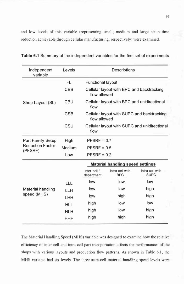
69

and low levels of this variable (representing small , medium and large setup time

reduction achievable through cellular manufacturing, respectively) were examined.

Table 6 . 1 Summary of the independent variables for the first set of experiments

I ndependent Levels Descriptions variable

FL Functional layout

CBB Cel lu lar layout with BPC and backtracking flow al lowed

Shop Layout (SL) CBU Cel lu lar layout with BPC and un id i rectional flow

CSB Cel lu lar layout with SUPC and backtracking flow a l lowed

CSU Cel lu lar layout with SUPC and un id i rectional flow

Part Fami ly Setup High PFSRF = 0.7 Reduction Factor Med ium PFSRF = 0 .5 (PFSRF)

Low PFSRF = 0.2

Material handl ing s�eed setti ngs

inter-cell / intra-cell with I ntra-cel l with deeartment SPC SUPC

LLL low low low

Material handl ing LLH low low high speed (MHS)

LHH low high h igh

HLL high low low

HLH h igh low high

HHH high h igh high

The Material Handling Speed (MHS) variable was designed to examine how the relative

efficiency of inter-cell and intra-cel l part transportation affects the performances of the

shops with various layouts and production flow patterns. As shown in Table 6 . 1 , the

MHS variable had six levels. The three intra-cel l material handling speed levels were

70

investigated at both high and low inter-cell / department material handling speed

settings.

Note that in a wel l-managed manufacturing shop, a single part should be able to be

handled more efficiently than a batch of parts. In other words, it is not l ikely that the

speed of moving parts in batches is faster than that of moving parts one piece by one

piece. Therefore, the MHS levels at which the material handl ing speed setting was high

for intra-cel l part movement with BPC and low for intra-cell part movement with SUPC

(i .e . LHL and HHL levels) were not investigated. The high and low settings for inter­

cell and intra-cell material handling speeds have been i l lustrated in Subsection 5 .5 .4 .

Thus, this set of experiments was based on the 5 x 3 x 6 ful l factorial design, with five,

three and six levels for the SL, PFSRF and MHS independent variables, respectively.

6.2 Selection of the Dependent Variables to be Measured

As summarised in Table 6.2, three dependent variables were used for evaluating the

shop performance, namely : average work-in-process inventory (A WIP), average flow

time (AFT) and average setup to processing time ratio (ASPTR). A WIP and AFT were

selected because they were considered two of the most important performance measures

for lIT manufacturing. The effectiveness of applying TIT techniques is eventually

reflected on the decrease of flow time. As wastes (defined in the broadest sense) are

being eliminated, delays in production processes are reduced and therefore, parts are

routed through production processes faster. In addition, existence of wastes in

production processes is best identified visual ly by the inventory level . As wastes happen,

parts are accumulated due to delays in production processes, and consequently, the

inventory level goes up. Although ASPTR is not directly related to shop performance,

it was selected particularly for evaluating the effectiveness of cellular manufacturing in

setup time reduction (Refer to Section 2 . 1 ) . Statistics on the results of the three

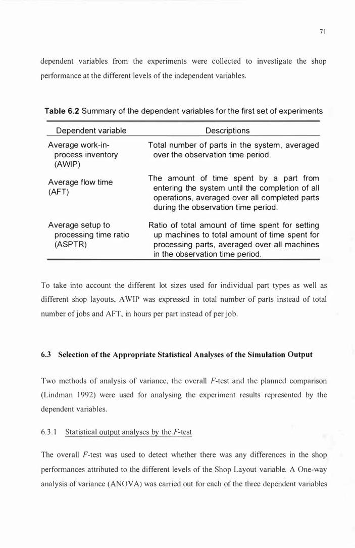
7 1

dependent variables from the experiments were collected to investigate the shop

performance at the different levels of the independent variables.

Table 6.2 Summary of the dependent variables for the first set of experiments

Dependent variable

Average work-in­process inventory (AWI P)

Average flow time (AFT)

Average setup to processing time ratio (ASPTR)

Descriptions

Total number of parts in the system, averaged over the observation time period .

The amount of time spent by a part from entering the system unti l the completion of a l l operations, averaged over a l l completed parts during the observation t ime period .

Ratio of total amount of t ime spent for setting up machines to total amount of t ime spent for processing parts , averaged over al l machines in the observation time period .

To take into account the different lot sizes used for individual part types as well as

different shop layouts, A WIP was expressed in total number of parts instead of total

number of jobs and AFT, in hours per part instead of per job.

6.3 Selection of the Appropriate Statistical Analyses of the Simulation Output

Two methods of analysis of variance, the overall F-test and the planned comparison

(Lindman 1 992) were used for analysing the experiment results represented by the

dependent variables.

6 .3 . 1 Statistical output analyses by the F-test

The overall F-test was used to detect whether there was any differences in the shop

performances attributed to the different levels of the Shop Layout variable. A One-way

analysis of variance (ANOVA) was carried out for each of the three dependent variables

72

at each of level of the PFSRF and MHS variables. Therefore in total 3x3x6 = 54

ANOV As were performed to achieve the results of overal l F-tests.

6 . 3 .2 Statistical output analyses by the planned comparison

The overall F-tests by ANOV As, however, were of limited use to this study because

they did not tel l where the differences came from if there were any. Therefore,

Lindman's planned comparison was used to pinpoint the causes of differences by

answering the fol lowing research questions, as put forward in Chapter 4 (Note that

Research question 4 was answered by the second set of experiments. ) :

Research question 1 : Do shop layout and part flow patterns have any influence on the

performance of a Kanban-controlled job shop? This question is addressed through the

following four sub-questions.

Sub-question 1 . 1 : For the cellular layout shops with batch production and

conveyance (BPC), is there any difference in performance between the shop with

backtracking flow al lowed and the shop with unidirectional flow ?

Sub-question 1 .2 : Simi lar to Sub-question 1 . 1 , but for the cellular layout shops with

single-unit production and conveyance (SUPC).

Sub-question 1 .3 : Among the shops with cellular layouts, are those with BPC

different from those with SUPC in their performance ?

Sub-question 1 .4 : I s there any difference between functional layout and cellular

layout in terms of shop performance ?

Research question 2 : How does the extent of setup time reduction through cellular

manufacturing affect the performances of the shops with the various layouts and

production flow patterns ?

Research question 3 : How does material handl ing speed affect the performances of the

shops with the various layouts and production flow patterns ?

73

To apply planned companson to answer the research questions, null hypotheses

corresponding to the research questions were first formulated. For example, sub­

question 1 . 1 is equivalent to investigating the truth of the statement: "For the cellular

layout shops with BPC, the shop performance with backtracking flow allowed is the

same as that with unidirectional flow". Since this statement has not yet been proved to

be true or false, it is a ' null hypothesis' . If the nul l hypothesis cannot be rejected ( i .e . is

true), we may conclude that there is no difference between the shop performances (or on

the contrary) . The null hypothesis for sub-question 1 , Ho( 1 a), can be expressed by the

following equation :

Ho( 1 a) : ).lCBB = ).lCBU, (6. 1 )

where ).lx = the population mean of the dependent variable studied at level x of the Shop

Layout independent variable, at each of the MHS and PFSRF levels. Similarly, the null

hypothesis for sub-question 1 .2 , Ho( 1 b), can be written as :

Ho( 1 b): ).lCSB = ).lCSU. (6.2)

Sub-question 1 .3 was answered by testing the null hypothesis:

Ho(2) : ).lCBB + ).lCBU = /lCSB + ).lcsu (6 .3)

If Ho(2) was true ( i .e . couldn't be rejected), no significant difference could be identified

between the cel lular layouts with batch production and conveyance ( i .e . CBB and CBU)

and those with single-unit production and conveyance (i .e . CSB and CSU). Hence, Sub­

question 1 .4 was answered by comparing the performance of the functional layout with

overall average performance of all the cel lular layouts and accordingly, the fol lowing

nul l hypothesis was tested:

Ho(3) : ).lFL = 1 I4( ).lCBB + /lCBU + ).lCSB + ).lcsu)· (6.4)

If Ho(3) was true (i .e . couldn't be rejected), no significant difference could be identified

between the cel lular layouts and the functional layout.

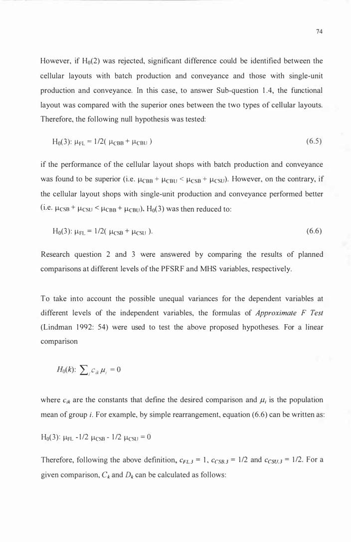
74

However, if Ho(2) was rejected, significant difference could be identified between the

cel lular layouts with batch production and conveyance and those with single-unit

production and conveyance. In this case, to answer Sub-question 1 .4, the functional

layout was compared with the superior ones between the two types of cellular layouts.

Therefore, the fol lowing null hypothesis was tested:

Ho(3) : �FL = 1 12( �eBB + �eBU ) (6 .5)

if the performance of the cel lular layout shops with batch production and conveyance

was found to be superior ( i .e . !leBB + !leBu < !lesB + !lesu). However, on the contrary, if

the cellular layout shops with single-unit production and conveyance performed better

( i .e . !lesB + !lesu < !leBB + !leBu), Ho(3) was then reduced to :

Ho(3 ) : !lFL = 1 12( !lesB + !lesu ) . C6.6)

Research question 2 and 3 were answered by comparmg the results of planned

comparisons at different levels of the PFSRF and MHS variables, respectively.

To take into account the possible unequal varlances for the dependent variables at

different levels of the independent variables, the formulas of Approximate F Test

(Lindman 1 992: 54) were used to test the above proposed hypotheses. For a l inear

comparison

where Cik are the constants that define the desired comparison and f.1i is the population

mean of group i. For example, by simple rearrangement, equation C6.6) can be written as :

Ho(3) : !lFL - 1 12 !lesB - 1 12 !lesu = 0

Therefore, fol lowing the above definition CFU = 1 , CCSB. 3 = 1 12 and CCSU, 3 = 1 12. For a

given comparison, Ck and Dk can be calculated as fol lows:

75

(6.7)

(6.8)

where X i- , a} and ni are the sample mean, variance and size of group i respectively.

Then approximately,

where F( I , d,_ ) is the F distribution with 1 degree of freedom in the numerator and dk

degrees of freedom in the denominator. dk is approximately

(6.9)

Let Fa( l .dd be the value of F to reach the a level of significance and p be the

probabil ity that

The null hypothesis, Ho(k), is rejected if and only if p � a .

In summary, unequal variances result in lower degrees of freedom and thus loss of some

power for the test. However, since a large sample size was adopted in this study, all

hypotheses were tested with high degrees of freedom (as shown in Appendix 1 0 and 1 4),

and thus high accuracy sti l l could be achieved for the planned comparisons.

76

CHAPTER 7

DEVELOPMENT AND OPERATION OF THE SIMULATION MODEL FOR THE

FmST SET OF EXPERIMENTS

In Chapter 5, we had described the design of the experimental system. In order to make

production runs so that the necessary statistics on the dependent variables for different

system conditions (Refer to Chapter 6) can be col lected, the designed experimental

system must actual ly be implemented.

In this study, simulation modelling was employed for system implementation. As

defined by Russell ( 1 990: 1 - 1 ), a simulation of a system is the operation of a model that

is a representation of the system. Therefore, to simulate the designed experimental

system, a simulation model of the system was first developed in the form of a

simulation program. Then, the simulation program, with input data corresponding to

different system conditions, was executed and statistics on the dependent variables were

col lected for further analysis. The development and operation of the simulation model

involved four parts: selection of the simulation language, development / coding of the

simulation model, verification of the simulation model and running the simulation

program. They will be i l lustrated individually below.

7.1 Selection of the Simulation Language

In order to select a suitable language for developing the simulation model, we must first

understand the differences between a simulation program and a general-purpose

program, such as a program coded in C, FORTRAN or BASIC language. The

differences are mainly in three aspects:

( l ) In a simulation program, concurrent execution of program modules is often

involved. For example, in a manufacturing shop with more than one machine, all

machines are running concurrently. Therefore, there must be a timing routine in the

77

background which controls the concurrent execution ( in simulated time) of the

routines for all machines. Similar examples are parts being processed

simultaneously, forklift trucks travel ling at the same time, etc.

(2) Queues are very often involved in a simulation program. For example, when a

container of parts arrives at a workstation, it has to be put in a queue if all machines

are busy at that time. Therefore, a mechanism for handling queues is required in a

simulation program.

(3) Usual ly, collection of the statistics of variables is necessary in a simulation program.

Some examples are average total number of parts in the system, average time spent

for machine setup, etc . A simulation program must support col lection of a variety of

statistics on variables.

Although al l the above differences can be coded by a general-purpose language as well ,

coding of these special functions is time consuming and the programmer needs

knowledge of the methods to implement these functions. On the other hand, simulation

languages support all these specific functions for simulation. A model builder needs not

to know the underlying principles for implementing these functions. Therefore,

development of a simulation model is more straightforward and effective with a

simulation language.

Considering the requirements for a simulation program, we selected SIMSCRl PT 1 1 . 5

general-purpose simulation language for developing the simulation model . Although

plenty of advanced simulation software packages other than SIMSCRlPT 1 1 .5 , such as

Promodel, Arena, AweSim, Witness, Simprocess, etc . are avai lable, we selected

SIMSCRlPT 1 1 .5 for the following reasons :

1 . It supports all the above mentioned special functions for a simulation program.

2 . Most of the other simulation packages are module-oriented. Although this feature

makes development of simulation models easier, particularly for those researchers

78

without programming background, some flexibil ity ill model development I S

usually sacrificed.

3 . On the other hand, the general-purpose nature o f S IMSCRIPT n . 5 similar to other

high-level languages, such as BASIC and FORTRAN, supports the programming of

complicated and fully customised logic and modell ing elements, which are

required for this study because of the complexity of the shop model .

4 . The English-l ike structure of S IMSCRIPT 1 1 .5 enables development and coding of

a simulation model at the same time. Model building is therefore made more

efficient.

Detai led descriptions of the SIMSCRIPT n . s simulation program developed for the

shop model will be presented in the next section.

7.2 Development / Coding of the Simulation Model

A S IMSCRI PT n . s program consists of three primary sections:

( 1 ) A preamble that declares the model ling elements used in the program,

(2) A main program where execution of statements begins, and

(3 ) Routines called by the main program or other routines.

The preamble and main progran1 will be i l lustrated in Subsections 7.2 . 1 and 7.2.2,

respectively. The routines for the four stages of model development will be described in

Subsections 7 .2 .3 through 7 .2 .6 .

7.2 . 1 Description of the preamble

The preamble is the first section of any SIMSCRIPT n . s program. It includes no

executable statements. All modell ing elements must be declared in the preamble. Four

modell ing elements, namely : processes, permanent entities, temporary entities and

79

global variables were declared in the preamble of our simulation program. They are

described as fol lows.

(a) Processes

In SIMSCRIPT I I .S , a process IS the pnmary dynamic model l ing element, which

represents an object and the sequence of actions it experiences throughout its l ife in the

model. There may be one or more instances (or copies) of a process during a simulation

run. The processes used in the shop model for this study are l isted in Table 7 . 1 .

Table 7 . 1 List of processes for the s imulation model

Process name Description

EXPERI MENT Generates mach ines and in itiates jobs into the system.

S I M . R U N . MASTER* Collects and resets statistics in a simulation run.

MAC H I N E Sets u p machines and processes parts.

SHIP .F ILD . CONTR Moves the containers filled with processed parts from the preceding workstation to the succeeding workstation.

RETN . E MPTY.CONTR Returns empty containers from the succeeding workstation to the preceding workstation.

S H I P . F ILD. CLCON Moves the containers filled with processed parts from the preced ing cell to the succeeding cel l .

RETN . EM PTY.CLCON Returns empty containers to the preceding cel l .

CMPL TD. CLCON Moves containers filled with completed parts to the receiving department

CMPL TD.CONTR Moves containers fi l led with processed parts to the cell outgoing storage area.

* SIMSCRIPT 1 1 . 5 al lows the use of periods in element names for easy identification.

For example, the MACHINE process represents the actions that a machine may carry

out for processing parts or setting up the machine. Since there were twenty-eight

machines in the simulated shop environment, an instance of the MACHINE process was

created to represent each machine. Each process declared in the preamble was further

80

described by a process routine. The process routine embodied the logic description of a

process. For example, the logic in the MACHINE process tells what actions to perform

when a container is emptied, when processing of a container of parts is completed, etc.

One unique feature of the process is the modell ing of the passing of time in the logic of

process routines. For example, in our shop model, the time for processing a part and the

time period that an idle machine had to wait ti l l the next container arrived were

model led in the MACHINE process. The functions of the processes used in the

simulation program of this study will be further described in Subsections 7.2 .3-6.

(b) Permanent entities

In SIMSCRIPT 1 1 . 5 , a permanent entity is used to represent a paSSIve static data

structure . Therefore, permanent entities are suitable for storing the data of system

parameters and configuration. Table 7.2 summarises the permanent entities used in the

shop model for this study.

Table 7.2 List of permanent entities for the simu lation model

Permanent entity name

MACH. ENTY

Description

Defines, for each mach ine:

- the mach ine ID, - the mach ine type, - the ID of the workstation where the machine is located, and - the ID of the cel l where the mach ine is located.

_ ..... _ ...... _--_ ...... _ .... _ ..... __ .. __ . __ .- ......... __ . __ ._._ .. _ .. _-------_ .... __ ...... -. __ .. _-_ .. -... __ ._ ..... _ .. __ ... __ ... _ .. _ .. _---_._-_ .. __ ._ .. _----

JOB. TYPE Defines the lot size for each part type.

JOB. TASK Defines, for each part type:

- the operation sequence, - the part family No. , - the numbers of intra-cell Kanban / container sets, - the numbers of inter-cell Kanban / container sets, and - the intra-cel l travel l ing distances

8 1

For example, as shown in Table 7.2, the MACH.ENTY permanent entity stored the

configuration data for machines. Since these data were static ( i .e. not to be manipulated)

throughout a simulation run, they were, therefore, stored in a permanent entity.

(c) Temporary entities

Temporary entities are used to model passive (as opposed to processes) dynamic objects.

They are passive because no action, logic or lapse of time is involved for temporary

entities. A temporary entity is similar to a data item. However, the data items

represented by temporary entities are dynamic. During the execution of the model, they

may be short-l ived ( i .e . may be destroyed sometime) or their numbers of instances ( i .e .

copies) may vary. In addition, a temporary entity may own a queue or be put in a queue.

Table 7 .3 shows the temporary entities used for the shop model of this study.

For example, the temporary entity, PROD.ORDER was used to model the work order

for an operation (processing a container of parts or setting up the machine) assigned to a

specific machine. When an operation was assigned, an instance of PROD.ORDER was

created. When the assigned operation was completed, the corresponding instance of

PROD.ORDER was then destroyed. Since the number of jobs ( i .e. containers of parts)

being processed in the system varied from time to time, the number of the instances of

PROD.ORDER also varied during the execution of the model . I n addition, when a

machine was busy, the instances of PROD. ORDER assigned to the machine had to be

put in a queue. Therefore, because of the dynamic nature of the work order, it was best

model led by a temporary entity.

(d) Global variables

In SI MSCRlPT n . s , a variable is either global or local in scope. The variables declared

in the preamble are global variables. They can be accessed by the main program and all

the routines. Variables can be defined in routines as wel l . However, variables defmed in

a routine are only temporary for that specific routine. When the routine is called, those

defined variables are created. When the routine is ended, the associated variables are

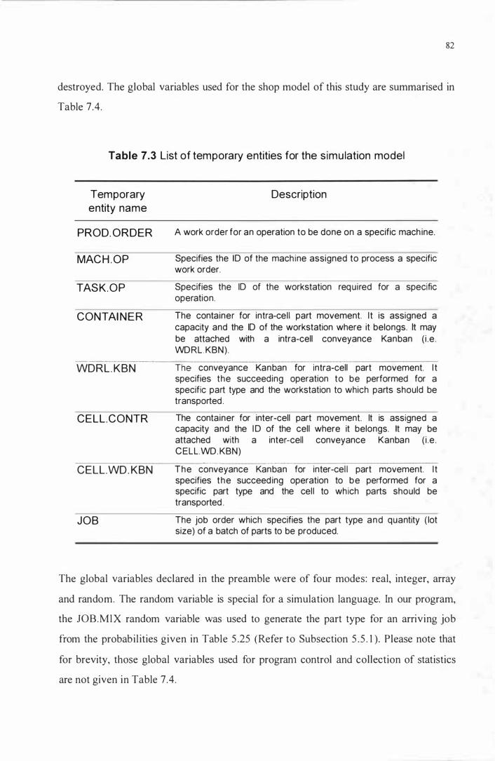
82

destroyed. The global variables used for the shop model of this study are summarised in

Table 7.4.

Table 7.3 List of temporary entities for the s imu lation model

Temporary entity name

PROD. ORDER

MAC H . OP

TASK.OP

CONTAI NER

Description

A work order for an operation to be done on a specific machine.

Specifies the ID of the mach ine assigned to process a specific work order.

Specifies the ID of the workstation required for a specific operation.

The container for intra-cel l part movement. I t is assigned a capacity and the ID of the workstation where it belongs. It may be attached with a intra-cell conveyance Kanban ( i .e . WDRL. KBN) .

---_._--_ .. . _-=-WDRL. KBN The conveyance Kanban for intra-cell part movement. I t

CELL.CONTR

specifies the succeeding operation to be performed for a specific part type and the workstation to which parts should be transported .

The container for inter-cell part movement. It is assigned a capacity and the ID of the cell where it belongs. It may be attached with a inter-cell conveyance Kanban ( i .e . CELL.WD. KBN)

._-_._--_. __ ._----_._ ... __ .. _-_ ....

CELL.WD. KBN The conveyance Kanban for inter-cel l part movement. I t specifies the succeeding operation to be performed for a specific part type and the cel l to wh ich parts should be transported .

JOB The job order which specifies the part type and quantity ( lot size) of a batch of parts to be produced.

The global variables declared in the preamble were of four modes: real, integer, array

and random. The random variable is special for a simulation language. In our program,

the JOB.MIX random variable was used to generate the part type for an arriving job

from the probabil ities given in Table 5 .25 (Refer to Subsection 5 .5 . 1 ). Please note that

for brevity, those global variables used for progran1 control and collection of statistics

are not given in Table 7.4.

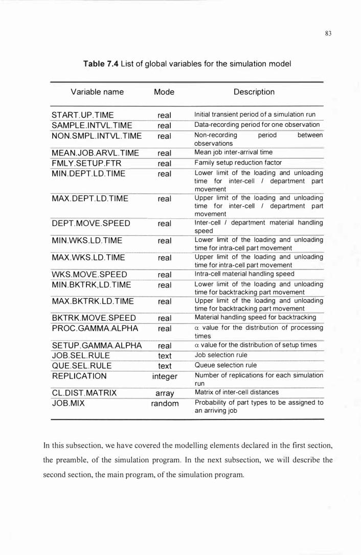
Table 7.4 List of g lobal variables for the simu lation model

Variable name

START UP.T IME SAMPLE . I NTVL.TIM E NON.SMPL. I NTVL.T IME

M EAN.JOB.ARVL.TIME FML Y .SETU P .FTR M I N . DEPT LD.TI ME

MAX. DEPT LD.TI M E

DEPT MOVE.SPEED

M I N .WKS . LD.TI M E _ .... _--_ .... __ .. _ .... __ ._-----_._-

MAX.WKS . LD.TIME

WKS. MOVE.SPEED M I N . BKTRK, LD.TI ME

MAX.BKTRK. LD.T IME

BKTRK.MOVE.SPEED PROC .GAMMA.ALPHA

SETU P . GAMMA.ALPHA JOB.SEL . RULE Q U E.SEL . RULE REPLICATION

CL .D IST MATRIX JOB.MIX

Mode

real real rea l

real real real

rea l

real

real

real

real rea l

rea l

rea l real

real text text

integer

array random

Description

I n itial transient period of a simulation run Data-record ing period for one observation Non-record ing period between observations Mean job inter-arrival time Family setup reduction factor Lower l imit of the load ing and un loading time for inter-cel l / department part movement Upper l imit of the loading and unload ing time for inter-cell / department part movement Inter-cell / department material handling speed Lower limit of the loading and unloading . time for intra-cell part movement Upper limit of the load ing and un loading time for intra-cell part movement Intra-cell material handling speed Lower l imit of the loading and unload ing time for backtracking part movement Upper l imit of the loading and unload ing time for backtracking part movement Material handling speed for backtracking ex value for the distribution of processing times ex value for the distribution of setup times Job selection rule Queue selection rule Number of replications for each simulation run Matrix of inter-cel l distances Probabil ity of part types to be assigned to an arriving job

83

In this subsection, we have covered the modelling elements declared in the fust section,

the preamble, of the simulation program. In the next subsection, we will describe the

second section, the main program, of the simulation program.

7.2 .2 Description of the main program and related routines

84

The main program is the first executable section of a S IMSCRIPT I I . S program. The

execution of the simulation program begins at the first statement of the main program.

The functions of the main program for the shop model we developed are given in Figure

7. 1 .

1 MAIN :

2 CALL READ . I N PUT . DATA r ou t i ne 3 CALL CREAT E . CONTR . W DKBN rou t i ne 4 CALL P R I NT . I N PUT . DATA r ou t i n e 5 CALL P R I N T . WS . D I S TANCE r ou t i n e 6 CALL P R I NT . CONT R . W DKBN rout i n e 7 ACT I VATE a S I M . RUN . MASTER p r o c e s s now 8 ACT I VATE an EXPERI MENT p r o c e s s now 9 s t a r t s imu l a t i on 1 0 E X I T MAI N .

Figure 7 .1 Description of the functions for the Main program

Note that in this subsection and the fol lowing subsections, we use a tool of structured

software design, namely, Structured Engl ish (Sommervi lle 1 996), to describe the

functions of the main program and routines. The program-like language of Structured

English is useful for communicating the actions and logic to be performed in a program

to programmers and nonprogrammers alike. However, for some special actions related

to simulation, we still used the original SIMSCRl PT I I .S commands (e.g. WAIT,

ACTIVATE, SUSPEND, etc . ) . In addition, we wi ll follow the S IMSCRIPT I I .S coding

convention of using capital letters for commands, routine names, variables and model

entities.

As shown in Figure 7 . 1 , the mam program has four functions: setting the system

configuration ( l ines 2-3), printing the system parameters (lines 4-6), initial ising

processes ( l ines 7-8) and starting simulation (l ine 9).

85

The input data was read and Kanban / container sets were created by cal ling the routines

at l ines 2 and 3 , respectively. For the purpose of verification, the input data, distance

matrices and created Kanban / container sets were printed out at l ines 4, 5 and 6,

respectively. At l ine 7, a S IM.RUN.MASTER process was activated for the control of

simulation replications. An EXPERIMENT process was activated ( l ine 8) for initiating

machines and job generation. The simulation run was then started at l ine 9. The

functions of the S IM.RUN.MASTER and EXPERIMENT processes are further

specified as fol lows.

The functions of the S IM.RUN.MASTER process routine are given in Figure 7.2. Note

that lines started with " " " (e.g. l ine 2) are remarks and not executable. In each

simulation run, the statistics on dependent variables were reset ( line 4) after waiting for

a initial transient time period ( l ine 3 ) . The REP EA T UNTIL loop ( lines 6- 1 3 ) performed

the replications for the simulation run. For each repl ication, the statistics on dependent

variables were collected and printed out (l ine 9) after waiting for a data-recording time

period (l ine 8). Each data-recording period was fol lowed by a non-recording period ( line

1 1 ) . The statistics on dependent variables were reset after each non-recording period

( line 1 2).

1 P ro c e s s S IM . RUN . MASTER :

2 " Handling the initial transient period 3 WAI T f o r S TART . U P . T I ME d a y s 4 CALL RE S E T . STAT I C S rout i ne

5 " Performing the replications 6 RE P EAT UNT I L a l l r e p l i c a t i on s comp l e t ed

7 " Collecting and printing statistics 8 WAI T f o r SAMPLE . I NTVL . T I ME d a y s 9 CALL P R I NT . RE S U L T S r out i n e

1 0 " Resetti ng statistics during non-recording period 1 1 WAI T NON . SM P L . I NTVL . T IME da y s 1 2 CALL RE S E T . STAT I ST I C S rout i n e 1 3 EN DRE PEAT 1 4 EX I T S IM . RUN . MASTE R .

Figure 7 .2 Description of the functions for the S I M . RU N . MASTER process

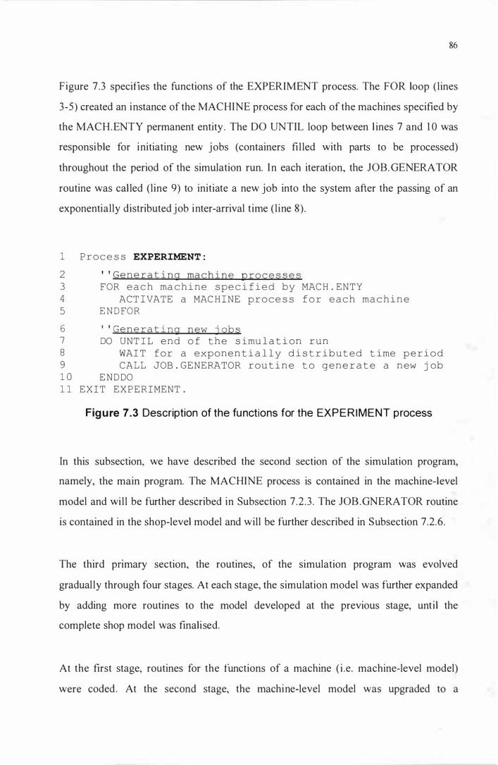
86

Figure 7.3 specifies the functions of the EXPERIMENT process. The FOR loop ( lines

3-5) created an instance of the MACHINE process for each of the machines specified by

the MACH.ENTY permanent entity . The DO UNTIL loop between l ines 7 and 1 0 was

responsible for initiating new jobs (containers fil led with parts to be processed)

throughout the period of the simulation run. I n each iteration, the JOB. GENERA TOR

routine was cal led (line 9) to initiate a new job into the system after the passing of an

exponentially distributed job inter-arrival time ( l ine 8) .

1 P r o c e s s EXPERIMENT :

2 ' ' GeneratinQ machine processes 3 FOR e a c h ma c h i ne s pe c i f i e d by MACH . ENTY 4 ACT I VATE a MAC H I NE p r o ce s s f o r e a c h ma c h i n e 5 E N D FOR

6 7 8 9 1 0

, ' GeneratinQ new jobs DO UNT I L end o f the s imu l a t i on run

WAI T for a exponen t i a l l y d i s t r i b u t e d t ime p e r i o d CALL JOB . GENERATOR rou t i n e t o g e n e r a t e a new j ob

E N D DO 1 1 E X I T E X P E R I MENT .

Fig u re 7.3 Description of the functions for the EXPERIMENT process

In this subsection, we have described the second section of the simulation program,

namely, the main program. The MACHINE process is contained in the machine-level

model and wil l be further described in Subsection 7 .2 .3 . The JOB.GNERATOR routine

is contained in the shop-level model and will be further described in Subsection 7.2.6.

The third pnmary section, the routines, of the simulation program was evolved

gradual ly through four stages. At each stage, the simulation model was further expanded

by adding more routines to the model developed at the previous stage, unti l the

complete shop model was finalised.

At the first stage, routines for the functions of a machine ( i .e. machine-level model)

were coded. At the second stage, the machine-level model was upgraded to a

87

workstation-Ievel model by adding routines supporting part movement between

workstations. The workstation-Ievel model was further upgraded to the cell-level model

at the third stage by adding routines supporting part movement between cel ls. Finally, at

the fourth stage, routines for handl ing arriving and completed jobs were added and the

complete shop-level model was achieved.

The functions of the routines supporting the models of the four development stages wil l

be described individual ly in Subsections 7 .2 .3-6. Please note that because of the large

number of routines developed for the simulation program, we are not intending to cover

all routines in the following subsections. Instead, only those routines necessary for

understanding the principle structure of the simulation program will be described in

detail . A full l isting of the source codes has been produced as a separate document.

7 .2 .3 Description of the machine-level model

At the stage of the machine-level model development the MACHINE process routine,

the CMPL TD.CONTR process routine and the QUE.MASTER routine were developed.

Their functions wi ll be described individually as follows.

(a) Description of the functions for the MACHINE process routine

The functions of the MACHINE process routine are given in Figure 7.4. The

MACHINE process was the 'engine' of the shop model because it was the only active

element that performed operations on parts and machine setups. Since machines exist

throughout the period of a simulation run, the machine process routine was an iterative

DO UNTIL loop between l ines 2 and 32 .

At the beginning of the DO UNTI L loop, the IF statement at l ine 3 checked whether

there was any work order assigned to this machine. If no work order was assigned to

this machine, then this MACHINE process was suspended ( l ine 30) . Note that

SUSPEND is a special S IMSCRlPT I I . S command uniquely for the purpose of

simulation control . Once the SUSPEND command is executed, the execution of the

88

process routine wil l be halted unti l the process is reactivated again. S ince the execution

of the process routine has been halted at the statement containing the SUSPEND

command, there is no way that the process routine can reactivate itself. In other words, a

suspended process routine can only be reactivated by other routines.

1 P ro c e s s MACHINE :

2 DO UNT I L end o f the s imu l a t i on run

3 I F a WORK . ORDER f o r t h i s MACH I N E found

4 " ProcessinG a container of Qarts 5 I F t h i s WORK . ORDER be ing for proce s s i ng a CONTAI N E R 6 REMOVE conveyance KANBAN f r om t h i s CONTA I NE R

7 ' ' ReturninG the conveyance Kanban 8 CALL C L R . KBN . POST r o u t i n e t o r e t u r n t h i s KANBAN 9 RE PEAT UNT I L t h i s CONTAINER emp t i e d 1 0 REMOVE a p a r t f rom t h i s CONA I N E R 1 1 PER FORM ope r a t i on on t h i s p a r t 1 2 PUT p r oce s s ed p a r t i n F I L LE D . CONTAI N E R 1 3 EN DRE P EAT

1 4 ' ' ReturninG the emQty container 1 5 ACT I VATE a RETN . EMPTY . CONTR p r o c e s s t o r e t u r n 1 6 t h i s EMPTY . CONTAI N E R

1 7 " HandlinG the filled container 1 8 ACT I VATE a CMPLT D . CONTR p r o c e s s t o h a n d l e t h i s 1 9 F I LLE D . CONTAINER 2 0 CALL QUE . MASTER rout i n e t o c he c k f o r n e x t j ob

2 1 ' ' A work order for settinG UQ the machine 2 2 E L S E 2 3 GET f u l l s e tup t ime f rom gamma d i s t r ibut i on 2 4 GET p a r t fami l y s e tup reduct i on f a c t o r 2 5 COMPUTE r educed s e t up t ime 2 6 PERFORM s e t up f o r t h i s MACH I N E 2 7 E N D I F

2 8 " NQ wQrk 2 9 E L S E 3 0 S U S PE N D 3 1 E N D I F 3 2 EN D DO 3 3 E X I T MACH I N E .

QrQ�r fQr :th� m��hin�

t h i s MAC H I NE

Figure 7.4 Description of the functions for the MAC H I N E process

89

In our simulation program, we implemented a mechanism for reactivating the

MACHINE process routine by initiating work orders (modelled by PROD.ORDER

temporary entities). Upon the issuing of a new work order to a specific machine, the

corresponding MACHINE process routine was reactivated. Once the suspended

MACHINE process routine was reactivated, the execution of the routine wil l continue

from the statement next to the SUSPEND statement ( i .e . l ine 3 1 in Figure 7.4) and the

DO UNTIL loop would be repeated again starting from the IF statement at l ine 3 . By

using this mechanism of suspending and reactivating the MACHINE process routine,

the idle state ( i .e . waiting for parts to be processed) of a machine can be model led.

As shown in Figure 7.4, if a work order for processing a container of parts was found

for this machine ( line 5), statements from l ine 6 to 20 would be executed. The

conveyance Kanban attached to the assigned container was removed ( l ine 6) and the

CLR.KBN.POST routine was cal led at l ine 8 to return the Kanban to the preceding

workstation. Then the REPEAT UNTIL loop ( l ines 9- 1 3 ) was executed for processing

parts unti l the assigned container was empty. Al l processed parts were stored in another

fil led container ( line 1 2) .

When the assigned container was emptied, a RETN.EMPTYCONTR process was

activated to return the empty container to the preceding workstation ( l ine 1 5) . Upon the

completion of processing al l parts, a CMPLTD.CONTR process was activated to move

the fil led container to the succeeding workstation ( l ine 1 8- 1 9) . The QUE.MASTER

routine was then cal led to check whether there was any container waiting to be

processed by this machine ( l ine 20). The CMPLTD.CONTR process routine and

QUE. MASTER routine wi l l be further described later.

If a work order for machine setup was found ( l ine 22), the statements for machine setup

(lines 23-26) were executed. After the completion of a work order, the DO UNTIL loop

was then repeated again to search for another work order for the machine ( line 3) .

(b) Description of the functions for the CMPL TD. CONTR process routine

90

The CMPLTD.CONTR process routine was called by the MACHINE process routine to

handle the container filled with processed parts . The functions of the CMPL TD.CONTR

process routine are shown in Figure 7 .5 . The processing status of the parts in the

container was checked to decide where to ship this filled container. If all necessary

operations were completed for the parts in the container ( line 3 ) ( i .e. A job had been

completed. ), a CMPLTD.CLCON process would be activated to move this container to

the shipping department ( l ines 4-5). The CMPLTD.CLCON was included in the shop­

level model and wil l be described in Subsection 7.2.6.

1 P r oc e s s CMPLTD . CONTR

2 " All oQerations f i n ished for the Qarts 3 I F a l l ope r a t i on s comp l e t ed f o r t h e F I LLE D . CONTA I N E R 4 ACT I VAT E a CM P LT D . C LCON p r o c e s s t o h a n d l e t h i s 5 F I L L E D . CONTA I N E R

6 " A container reguirinQ intra-cel l movement 7 E L S E , I F t h i s F I L LE D . CONTAI NER t o be s hi p p e d t o 8 s u c c e e d i n g wo r k s t a t i on i n t h e c e l l

9 I F a conveyance KANBAN a va i l ab l e f o r moveme n t 1 0 ATTACH t h i s KANBAN t o t h i s F I LLE D . CONTAINER 1 1 ACT I VATE a S H I P . FI L D . CONTR p ro c e s s t o s h i p t h i s 1 2 F I LLE D . CONTA I N E R 1 3 E L S E 1 4 PUT t h i s F I L LE D . CONTAI N E R i n o u t p u t b u f f e r 1 5 E N D I F

1 6 ' ' A container reguirinQ inter -cell movement 1 7 E L S E , I F t h i s F I L LE D . CONTA I N E R t o b e s h ipped t o 1 8 s u c c e e d i n g c e l l 1 9 I F a conveyance KANBAN a va i l a b l e f o r moveme n t 2 0 ATTACH t h i s KANBAN t o t h i s F I L L E D . CONTAI N E R 2 1 ACT I VATE a S H I P . F I L D . C LCON p r o ce s s t o s h i p t h i s 2 2 FI L L E D . CONTA I NER 2 3 E L S E 2 4

2 5

2 6

PUT thi s F I LLE D . CONTAINER in ce l l outgo i ng s t o rage E N D I F

EN D I F 2 7 EX I T CMPLT D . CONTR

Figure 7.5 Description of the functions for the CMPL TD.CONTR process

If the fil led container was to be moved to a succeeding workstation in the cell ( l ines 7-8),

the statement at l ine 9 searched for a conveyance Kanban authorising the movement of

9 1

this container. I f an available conveyance Kanban was found, the Kanban was then

attached to this fil led container ( l ine 1 0) and a SHIP.FILD.CONTR process was

activated ( l ines 1 1 - 1 2) to move this container to the succeeding workstation designated

by the Kanban. However, if no conveyance Kanban for authorising the movement of

this container was found ( line 1 3 ), this fi l led container would be queued in the output

buffer of the workstation. The SHIP.FILD.CONTR process was included in the

workstation-Ievel model and wil l be described in Subsection 7 .2.4.

I f the fil led container was to be moved to a succeeding workstation in another cell ( l ines

1 7 - 1 8), the statement at l ine 1 9 first checked if a corresponding conveyance Kanban was

available for authorising the movement. If an available Kanban was found, the Kanban

would be attached to this fil led container (l ine 20) and a SHIP .FILD.CLCON process

was activated ( lines 2 1 -22) to ship this fi l led container to the succeeding workstation

designated by the Kanban. However, if no available conveyance Kanban for authorising

this movement could be found ( l ine 23), this fi l led container would be queued in the

outgoing storage of the cell (24). Since the SHIP.FILD.CLCON process involved inter­

cell movement, it was included in the cell-level model and will be described in

Subsection 7 .2 .5 .

(c) Description of the functions for the QUE. MASTER routine

The functions of the QUE.MASTER routine cal led by the MACH INE process routine

are presented in Figure 7.6. The functions of the QUE.MASTER routine were to select a

fil led container which was waiting to be processed by a specific machine, and to issue

work orders to the machine for processing the selected container.

As shown in F igure 7 .6, the REPEAT FOR loop (l ines 2- 1 8) was executed to for each

fil led container waiting to be processed by the machine in the input buffer. Recal l that

for the Kanban system employed in this study, empty containers also served as

production Kanbans (Refer to Subsection 5 .5 .2) . I n other words, the processing of a

container of pats could only be initiated when there was a corresponding empty

92

container available for storing the processed parts. Therefore, the I F statement at l ines 5-

6 checked for an available empty container for storing the processed parts.

1 Rout i n e QUE . MASTER :

2 RE P EAT FOR e a c h F I LLE D . CONTAI NER i n input bu f fe r 3 r e qu i r i n g t h i s MAC H I N E

4 5 6 7

8 9 1 0

1 1 1 2 1 3 1 4

1 5

1 6 1 7 1 8 1 9 2 0 2 1 2 2

" Searching for the job with highest priority I F an EMPTY . CONTAI NE R ava i l a b l e f o r s to r i ng proce s s e d

pa r t s f r om t h i s F I L LE D . CONTA I N E R COM PUTE queue p r i o r i t y f o r t h i s F I LLE D . CONTA I N E R COM PUTE j ob p r i o r i t y f o r t h i s F I L LE D . CONTA I NE R I F queue p r i o r i t y GREATE R T HAN p r e v i ous one

S E T t h i s F I LLE D . CONTAI NE R as NEXT . CONTAI NE R E L S E I F queue p r i o r i t y EQUAL p r e v i o u s o n e

I F j ob p r i o r i t y GREAT E R T HAN p re v i ou s o n e SET t h i s F I LLE D . CONTA I N E R a s

NEXT . CONTA I NE R E N D I F

E N D I F E N D I F

EN DRE PEAT I F a NEXT . CONTAI NE R found

PUT WORK . ORDER f o r s e t t i ng up t h i s MAC H I NE PUT WORK . ORDER f o r p r o ce s s i ng t h i s F I NAL . CONTA I N E R on

t h i s MAC H I N E 2 3 AS S I GN t h i s F I NAL . CONTA I NER and t h i s EMPTY . CONTA I N ER 2 4 t o t h i s MACH I NE 2 5 E N D I F 2 6 EX I T QUE . MASTER .

Figure 7.6 Description of the functions for the QUE .MASTER routine

Recall that both the repetitive-lots queue selection rule and the shortest processing time

(SPT) job selection rule were used in the shop environment for job scheduling (Refer to

Subsection 5 . 5 . 3 (b)). Therefore, if an available empty container was found (l ines 5-6)

for the specific fil led container in the input buffer, both the priority values for queue

selection ( l ine 7) and job selection ( line 8) were calculated. If the queue selection

priority value of the current fil led container was higher than the previous one, the

current fil led container would be designated as the next container (the container to be

processed next) ( lines 9- 1 0). Also, if the current filled container has a queue selection

93

priority value equal to the previous one but a higher job selection priority value ( l ine 1 1 -

1 2), the current fil led container was also designated as the next container ( lines 1 3- 1 4) .

If a next container could be selected ( line 1 9), the work orders for setting up the

machine ( line 20) and processing parts (l ines 2 1 -22) would be initiated. Both the

selected next container and the corresponding empty container were assigned to the

machine ( lines 23-24) .

I n the machine-level model, the interactions (movement of containers and Kanbans)

among different instances of the MACHINE process were handled by five routines.

Three of the five routines, namely: CLR.KBN.POST routine ( l ine 8 in F igure 7.4),

SHIP .FILD.CONTR process routine (l ine 1 1 III Figure 7 .5) and

RETN.EMPTY.CONTR process routine ( l ine 1 5 in Figure 7.4) handled the interactions

among workstations in a cel l . Therefore, they were developed at the stage of

workstation-Ievel model development and wil l be described in detail in the next

subsection.

Another routine, the SHIP.FILD.CLCON process routine handled the movement of

fi l led containers between cel ls. Therefore, it was developed at the stage of cell-level

model development and will be described in detail in Subsection 7 .2 .5 . The last routine,

CMPLTD.CLCON process routine, handled the movement of containers between cells

and the shipping department. It was therefore developed at the stage of shop-level model

development and will be described in detail in Subsection 7.2.6.

7.2.4 Description of the workstation-level model

At this stage of model development, three more routines were added to upgrade the

machine-level model developed at the previous stage to the workstation-level model .

The three routines added, namely: CLR.KBN.POST routine, SHIP.FILD.CONTR

process routine and RETN.EMPTY.CONTR process routine supported the movement of

94

containers (empty or fi l led) and conveyance Kanbans among workstations in a cel l .

They will be described individual ly below.

(a) Description of the functions for the CLR.KBN.POST routine

The functions of the CLR.KBN.POST routine are presented in Figure 7 .7 . This routine

was responsible for returning the conveyance Kanban removed from a fi lled container to

the preceding workstation.

1 Rou t i ne CLR . KBN . POST :

2 " A Kanban for inter-cell part movement 3 I F t h i s Kanban f o r i n t e r - c e l l p a r t movemen t 4 CALL RETN . CL . W DKBN rout i ne f o r r e t urning t h i s KANBAN 5 t o p r e c e d i n g c e l l 6 ' ' A Kanban for intra-cell part movement 7 E L S E 8 MOVE t h i s KANBAN t o p r e c e d i n g wo r k s t a t i on

9 I F a F I LL E D . CONTAINER de s i gnated f o r t h i s KANBAN found 1 0 i n output bu f f e r 1 1 ATTACH t h i s KANBAN t o t h i s FI LLE D . CONTA I NE R 1 2 ACT I VATE a S H I P . FI L D . CONTR p roce s s t o move 1 3 t h i s F I LLE D . CONTA I NER to s u cceeding wo r k s t a t i on 1 4 E L S E

1 5 ' ' No container waiting for the Kanban 1 6 PUT t h i s KANBAN i n Kanban queue 1 7 E N D I F 1 8 E N D I F 1 9 EX I T CLR . KBN . POST .

Figure 7.7 Description of the functions for the CLR .KBN. POST routine

As shown in Figure 7 .7, If the conveyance Kanban was to be returned to a preceding

workstation in another cell (line 3 ), the RETN.CL.WDKBN routine was cal led ( lines 4-

5) for returning this Kanban. Otherwise, this Kanban was returned to the preceding

workstation in the cell ( l ine 8). The functions of the RETN.CL.WDKBN routine will be

described in Subsection 7 .2 .5 .

95

Recall that for the Kanban system employed in the shop environment modelled, a

conveyance Kanban was used to authorise the movement of a container fil led with

processed parts to the succeeding workstation (Refer to Subsection 5 . 5 .2) . Therefore, as

shown in Figure 7.7, upon the arrival of the returned Kanban at a workstation, the filled

containers queued in the output buffer were scanned ( lines 9- 1 0) to find one waiting for

the authorisation of this Kanban for movement. If no fi l led container associated with

this Kanban was found ( line 1 5), the Kanban was then queued in the Kanban queue ( line

1 6) .

If a fi l led container requiring the returned Kanban was found, this Kanban would be

attached to this fil led container ( line 1 1 ) and a SHIP .FILD.CONTR process was

activated ( lines 1 2- 1 3 ) to move this authorised container to the succeeding workstation.

The functions of the SHIP.FILD.CONTR process routine will be described next.

(b) Description of the functions for the SHIP.FILD.CONTR process routine

The SHIP.FILD.CONTR process was responsible for moving a container fil led with

parts to be processed to the succeeding workstation. The functions of the

SHIP.FILD.CONTR process routine are presented in Figure 7 .8 . I f the fil led container

was to be moved to a succeeding workstation in another cell ( l ine 3 ), a

SHIP.FILD.CLCON process was activated (l ines 4-5) for moving this fil led container;

otherwise, the fil led container was moved to the succeeding workstation in the cell ( line

8). The functions of the SHIP.FILD.CLCON process routine wil l be further described in

Subsection 7 .2 .5 .

Upon the arrival of a filled container at the succeeding workstation, the I F statement at

l ines 9- 1 0 checked whether there was any empty container available for storing the

processed parts from the fil led container (Recall that empty containers were also

production Kanbans authorising the processing of parts). If no available empty container

was found ( line 25), the fil led container would be queued in the input buffer of the

workstation ( line 26).

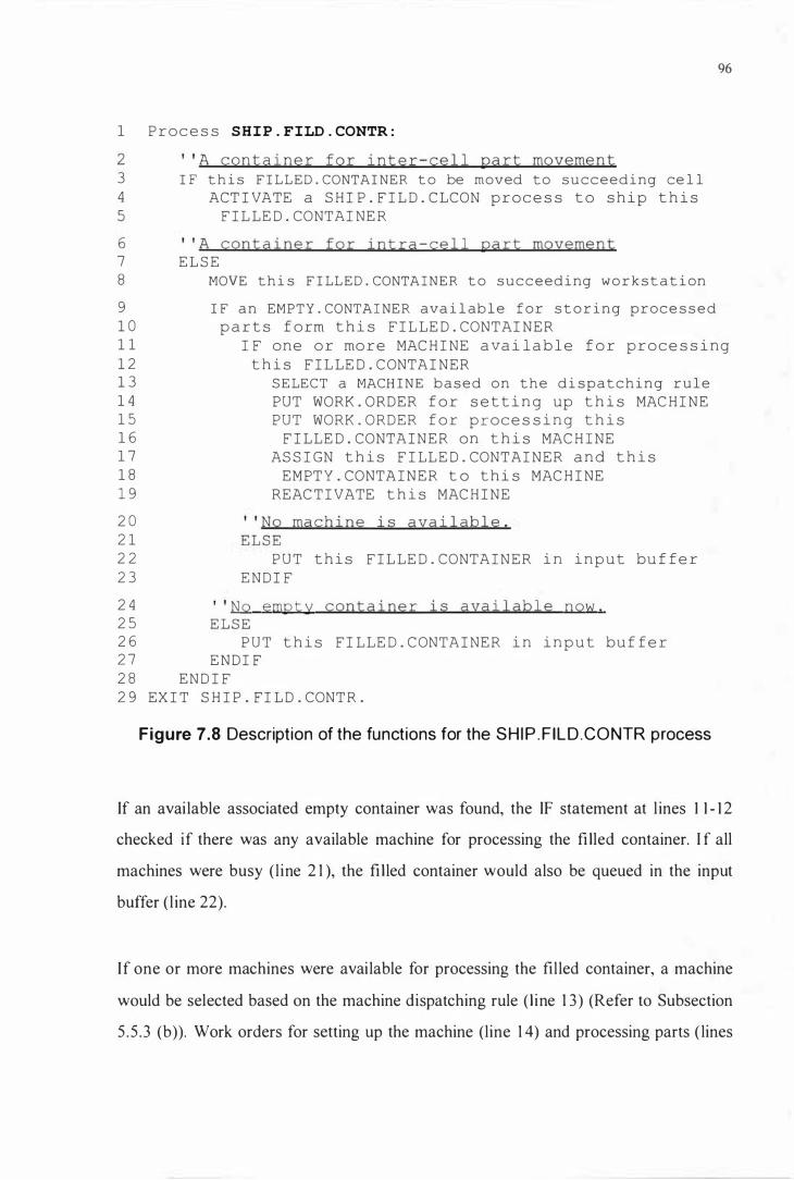
1 P r o c e s s S H I P . FILD . CONTR :

2 ' ' A container for inter -cell Qart movement 3 I F t h i s F I L L E D . CONTAI NER t o be moved t o s u c c e e d i ng ce l l 4 ACT I VATE a S H I P . F I L D . C LCON p r o c e s s t o s h i p t h i s 5 F I L LE D . CONTAI NE R

6 " A container for intra-cell part movement 7 E L S E 8 MOVE t h i s F I LL E D . CONTA I N E R t o s u c c e e d i ng w o r k s t a t i on

9 I F a n EMPTY . CONTAI NE R ava i l ab l e f o r s t o r i n g p r o c e s s e d 1 0 p a r t s f orm t h i s F I L LE D . CONTAI NER

96

1 1 I F one o r mo re MAC H I NE a va i l a b l e f o r p r o ce s s i ng 1 2 t h i s F I L LE D . CONTAI NER 1 3 S E LECT a MACH I N E b a s e d on t h e d i s p a t c h i n g r u l e 1 4 PUT WORK . ORDER f o r s e t t i n g up t h i s MAC H I NE 1 5 PUT WORK . ORDER f o r proce s s i n g t h i s 1 6 F I LLE D . CONTA I N E R on t h i s MAC H I NE 1 7 AS S I GN t h i s F I LLE D . CONTAI NER a n d t h i s 1 8 EMPT Y . CONTA I N E R t o t h i s MAC H I NE 1 9 REAC T I VATE t h i s MAC H I NE

2 0 2 1 2 2

2 3

2 4 2 5 2 6 2 7

2 8

, ' No mach i ne is avai lable . E L S E

P U T t h i s F I L LE D . CONTA I N E R i n i n p u t bu f fe r E N D I F

" No empty container is available now . E L S E

P U T t h i s F I LLE D . CONTA I NE R i n i n p u t bu f fe r E N D I F

EN D I F 2 9 EX I T S H I P . FI L D . CONT R .

Figure 7.8 Description of the functions for the SHI P . F ILD.CONTR process

If an avai lable associated empty container was found, the IF statement at l ines 1 1 - 1 2

checked if there was any available machine for processing the fi lled container. I f all

machines were busy ( l ine 2 1 ), the fi l led container would also be queued in the input

buffer ( l ine 22).

If one or more machines were avai lable for processing the filled container, a machine

would be selected based on the machine dispatching rule ( l ine 1 3 ) (Refer to Subsection

5 .5 .3 (b)). Work orders for setting up the machine (line 1 4) and processing parts ( lines

97

1 5- 1 6) would then be issued. Both the fi l led container and the associated empty

container were assigned to this selected machine ( l ines 1 7- 1 8) .

As described in Subsection 7 .2 .3 , when a machine was idle, the corresponding instance

of the MACHINE process was suspended. Therefore, after the necessary work orders

were issued, the instance of the MACHINE process for the selected machine had to be

reactivated ( l ine 1 9) . As shown in Figure 7.4, after the reactivation of a MACHINE

process routine, the execution of the routine would be resumed from l ine 3 1 . Therefore,

the DO UNTIL loop would be repeated again from line 2 in the MACHINE process

routine and the assigned work orders were processed as described in Subsection 7 .2 .3 .

(c) Description of the functions for the RETN.EMPTY.CONTR process routine

The RETN.EMPTYCONTR process handled the returning of empty containers from

the succeeding workstation to the preceding workstation. The functions of the

RETN.EMPTYCONTR process routine are shown in Figure 7.9. If the empty container

was to be returned to a proceeding workstation in another cel l ( line 3 ), a

RETN.EMPTYCLCON process was activated ( lines 4-5) for returning this container.

S ince an empty container for inter-cell part movement had been returned, a space in the

input buffer was available for storing another container fil led with parts to be processed

from another cell . Therefore, the statement at l ine 7 checked the cell incoming storage

(where fil led containers from another cell were temporari ly held) to find a fil led

container for the same part type as that for the returned empty container. If a matching

fi lled container was found, a SHIP .FILD.CONTR process would be activated ( lines 9-

1 0) to move this fi l led container to this workstation.

If the empty container was to be returned to a preceding workstation in the cell ( l ine 1 3),

it would be moved to the preceding workstation (line 1 4) . As i l lustrated in Subsection

5 . 5 .2, an empty container also served as a production Kanban for authorising the

processing of a specific fil led container. Therefore, the statement at l ines 1 5- 1 6 checked

98

whether this empty container was required for processing any filled container in the

input buffer of this workstation. If this empty container was not required at that time

( line 27), it would be queued in the container queue (l ine 28) .

1 P r o c e s s RETN . EMPTY . CONTR :

2 ' ' A container for inter-cell Qart movement 3 I F t h i s E M P T Y . C ONTA I N E R b e i n g f r om p r e c e d i n g c e l l 4 ACT I VATE a RETN . EM PT Y . C LC ON p r o c e s s t o r e t u r n t h i s 5 EMPTY . C ONTA I N E R t o p r e c e d i n g c e l l

6 " Searching the incoming storage for a new container 7 I F t h e a va i l a b l e i n p u t bu f f e r s p a c e ma t ch i ng a 8 F I L LE D . CONTA I N E R wa i t i ng i n c e l l i n c omi n g s t o r a g e 9 ACT I VATE a S H I P . F I L D . CONTR p r o c e s s t o move t h i s 1 0 F I L LE D . CONTA I N ER t o t h i s wo r k s t a t i on 1 1 E N D I F

1 2 ' ' A contai ner for intra-cell Qart movement 1 3 E L S E 1 4 MOVE t h i s EMPTY . CONTA I NE R t o p r e ce d i n g w o r k s t a t i on

1 5 I F t h i s EMPTY . CONTA I N E R r e q u i r e d f o r p r o c e s s i ng a 1 6 F I LLE D . CONTA I N E R i n i np u t b u f f e r 1 7 I F o n e o r mo r e MAC H I N E a va i l a b l e f o r p r o ce s s i ng 1 8 t h i s F I L LE D . CONTA I N E R 1 9 S E LECT a MACH I N E b a s e d on the d i s p a t c h i n g r u l e 2 0 P U T WORK . ORDER f o r s e t t i n g up t h i s MAC H I N E 2 1 PUT WORK . ORDER f o r p r o c e s s i ng t h i s 2 2 F I LLE D . CONTA I N E R o n t h i s MAC H I NE 2 3 AS S I GN t h i s F I L LE D . CONTA I N E R a n d t h i s 2 4 EMPTY . CONTA I N E R t o t h i s MAC H I N E 2 5 REACT I VAT E t h i s MAC H I N E

2 6 " No machine is available . 2 7 E L S E 2 8 PUT t h i s EMPTY . CONTA I N E R i n c o n t a i n e r queue 2 9 E N D I F

3 0 3 1 3 2 3 3 3 4

" T he emQty contai ner is not required now . E L S E

P U T t h i s EMPTY . C ONTA I NE R i n c on t a i n e r q u e u e E N D I F

E N D I F 3 5 EX I T RETN . EMPTY . CONTR .

Figure 7.9 Description of the functions for the RETN . EMPTY.CONTR process

99

I f a fil led container waiting for this empty container was found, the IF statement at l ines

1 7 - 1 8 checked if there was any avai lable machine for processing the fil led container. I f

all machines were busy ( l ine 27), the empty container would also be queued in the

container queue ( l ine 28) .

However, if one or more machines were avai lable for processing the fi lled container, a

machine would be selected based on the machine dispatching rule ( line 1 9) (Refer to

Subsection 5 . 5 .3 (b)). Work orders for setting up the machine ( line 20) and processing

parts ( l ines 2 1 -22) would then be issued. Both the empty container and the associated

filled container were assigned to this selected machine ( l ines 23-24). As described for

the SHIP .F ILD.CONTR process routine, the instance of the MAC H INE process for the

selected machine had to be reactivated ( line 25) to resume the execution of the process

routine.

At this stage of model development, the workstation-Ievel model was evolved by adding

three routines to the machine-level model developed at the first stage. I n addition, three

routines, namely: RETN.CL.WDKBN routine, SHIP .FILD.CLCON process routine and

RETN.EMPTY.CLCON process routine, were called for handling the interactions

among cells . They will be further described in the next section.

7 .2 .5 Description of the Cel l-level model

The workstation-level model developed in the work described above was next upgraded

to the cell -level model . Three routines, namely, RETN.CL.WDKBN routine,

SHIP.FILD.CLCON process routine and RETN.EMPTY.CLCON process routine, were

added to the simulation program. These routines supported the movement of Kanbans

and containers (empty or fil led) among cells in the shop. Their functions will be

described in detail as fol lows.

Ca) Description of the functions for the RETN.CL.WDKBN routine

1 00

The RETN .CL.WDKBN routine was cal led by the CLR.KBN.POST routine (See

Subsection 7 .2 .4 (a)) to return a conveyance Kanban to a preceding workstation in

another cell or to the receiving department (where job orders were issued) . The

functions of the RETN.CL.WDKBN routine are presented in Figure 7. 1 0.

1 Rou t i ne RETN . CL . WDKBN

2 MOVE t h i s KAN BAN t o p r e c e d i n g c e l l / r e c e i v i n g dept .

3 I F a F I LL E D . CONTA I N E R de s i gnated f o r t h i s KANBAN f ound 4 i n o u t g o i n g s t o r a g e 5 ATTACH t h i s KANBAN t o t h i s F I L LE D . C ONTA I NE R 6 ACT I VAT E a S H I P . F I L D . C LCON p r o c e s s t o move t h i s 7 F I L LE D . CONTA I NE R t o s u c c e e d i n g c e l l 8 E L S E

9 1 0

1 1

" No container waiting for the Kanban PUT t h i s KANBAN i n K a nb a n queue

E N D I F 1 2 EX I T RETN . C L . W DKBN

Figure 7. 1 0 Description of the functions for the RETN .CL.WDKBN routine

When the Kanban was returned to the preceding workstation I receiving department

( l ine 2), the statement at l ines 3 -4 checked the fil led containers at the outgoing storage

of the cel l I receiving department to see whether any container could be authorised for

movement by this Kanban. (Recall that a conveyance Kanban was used to authorise the

movement of a fil led container from a preceding workstation to the succeeding

workstation). If no container was waiting for the authorisation by this Kanban (l ine 8),

this returned Kanban will be queued in the Kanban queue ( line 1 0) .

On the other hand, if a fi l led container waiting authorisation by this Kanban was found,

the Kanban would be attached to this fil led container (l ine 5) . A SHIP.FILD.CLCON

process was then activated ( l ines 6-7) to move this filled container to the succeeding

workstation.

(b) Description of the functions for the SHIP.FILD.CLCON process routine

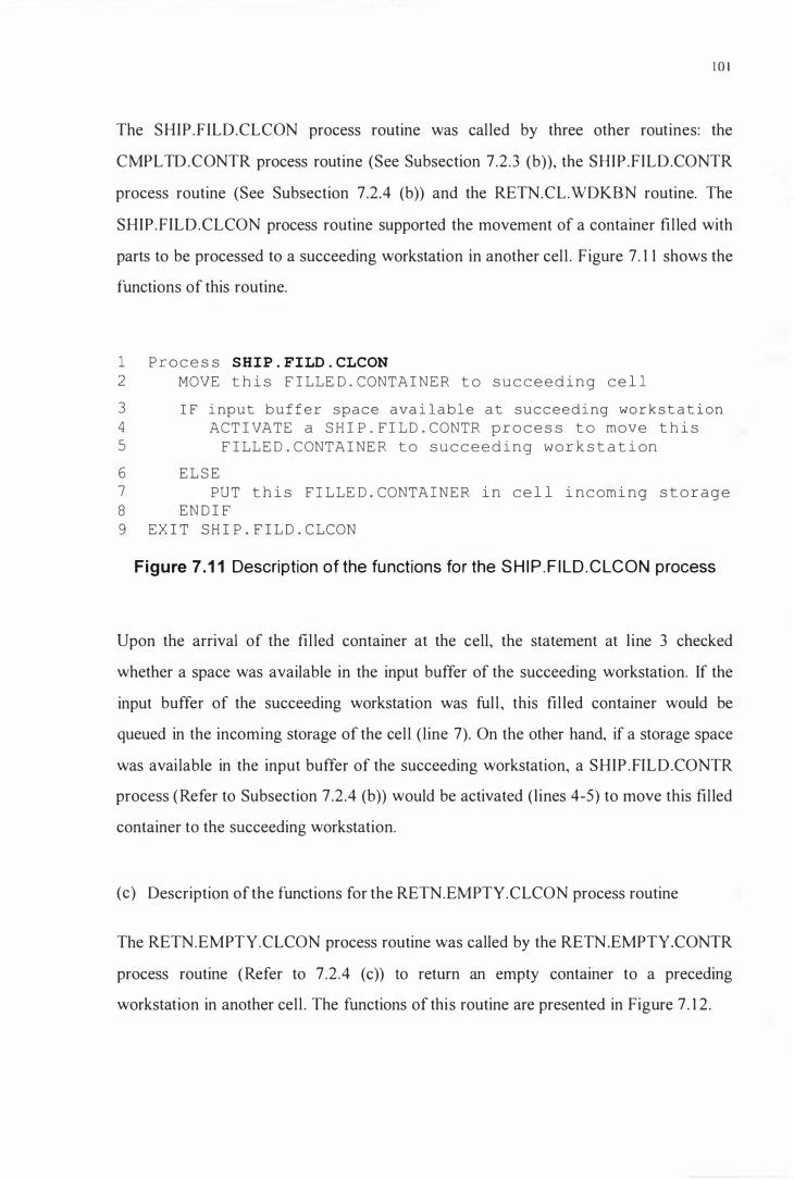
1 0 1

The SHIP .FILD.CLCON process routine was cal led by three other routines: the

CMPLTD.CONTR process routine (See Subsection 7 .2 .3 (b)), the SHIP .FILD.CONTR

process routine (See Subsection 7.2.4 (b)) and the RETN.CL.WDKBN routine. The

SHIP .FILD.CLCON process routine supported the movement of a container fil led with

parts to be processed to a succeeding workstation in another cel l . Figure 7. 1 1 shows the

functions of this routine.

1 P r o c e s s SHIP . FILD . CLCON

2 MOVE t h i s F I LLE D . CONTA I N E R t o s u c c e e d i n g c e l l

3 I F i nput b u f f e r space ava i l a b l e a t s u c c e e d i ng wo r k s t a t i on 4 ACT I VATE a S H I P . F I L D . CONTR p r o c e s s t o move t h i s 5 F I LL E D . C ONTA I NE R t o s u c c e e d i n g w o r k s t a t i on

6 E L S E 7 PUT t h i s F I L LE D . CONTA I N E R i n c e l l i n c omi ng s t o r a g e 8 EN D I F 9 EX I T S H I P . F I L D . C LCON

Figure 7 . 1 1 Description of the functions for the S H I P . F I LD .CLCON process

Upon the arrival of the fil led container at the cell, the statement at l ine 3 checked

whether a space was available in the input buffer of the succeeding workstation. If the

input buffer of the succeeding workstation was ful l , this fil led container would be

queued in the incoming storage of the cel l ( line 7). On the other hand, if a storage space

was avai lable in the input buffer of the succeeding workstation, a SHIP .FILD.CONTR

process (Refer to Subsection 7.2 .4 (b)) would be activated (lines 4-5) to move this fil led

container to the succeeding workstation.

(c) Description of the functions for the RETN.EMPTY.CLCON process routine

The RETN.EMPTY.CLCON process routine was called by the RETN.EMPTY.CONTR

process routine (Refer to 7.2 .4 (c)) to return an empty container to a preceding

workstation in another cel l . The functions of this routine are presented in Figure 7 . 1 2 .

1 P r o ce s s RETN . EMPTY . CLCON

2 " Container for storing raw material parts 3 I F t h i s EMPT Y . CONTA I N E R being f r om t h e r e c e i v i n g dept . 4 MOVE t h i s EMPTY . CONTA I N E R t o r e c e i v i ng dept .

5 I F t h i s EMPTY . CONTAINER r e qu i red b y a queued JOB 6 F I LL t h i s EMPTY . CONTA I N E R w i th r aw mat e r i a l p a r t s 7 requ i red f o r s t a r t ing t h i s JOB

8 I F a conveyance KANBAN a va i l a b l e f o r a u t ho r i s i ng 9 movement o f t h i s F I L L E D . CONTA I N E R 1 0 ATTACH t h i s KANBAN t o t h i s F I L L E D . CONTA I NER

1 02

1 1 ACT I VATE a S H I P . F I L D . C LCON proce s s t o move t h i s 1 2 F I LLE D . CONTAINER t o succeeding ce l l

1 3 E L S E 1 4 " No conveyance Kanban available for shipment 1 5 PUT t h i s F I L L E D . CONTAI N E R i n out g o i ng s t o rage 1 6 EN D I F

1 7 E L S E 1 8 " The empty container not required now 1 9 PUT t h i s EMPT Y . CONTAINER i n cont a i ne r queue 2 0 END I F

2 1 E L S E 2 2 " Container for storing intermediate parts 2 3 MOVE t h i s EMPT Y . CONTAI NE R t o p r e c e d i n g ce l l

2 4 I F t h i s EMPTY . CONTAINER requi red f o r s to r i ng 2 5 p r o ce s s e d pa r t s f r om a F I L L E D . CONTAINER i n i nput 2 6 bu f fe r o f p r e ceding wo r k s t a t i on

2 7 I F one o r more MAC H I N E ava i l a b l e f o r p ro ce s s i ng 2 8 t h i s F I LLE D . CONTAINER 2 9 SELECT a MAC H I N E b a s e d on the d i s p a t ching r u l e 3 0 PUT WORK . ORDER f o r s e t t ing up t h i s MACH I NE 3 1 PUT WORK . ORDER f o r p r o ce s s i ng t h i s 3 2 F I LLE D . CONTA I NER on t h i s MACH I N E 3 3 AS S I GN t h i s F I LLE D . CONTA I N E R a n d t h i s 3 4 EMPTY . CONTAI N E R t o t h i s ma chine 3 5 REACT I VATE thi s MACH I NE

3 6 E L S E 3 7 ' ' No machi ne is avai lable . 3 8 PUT t h i s EMPTY . CONTA I N ER i n c on t a i n e r queue 3 9 EN D I F

4 0 E LS E 4 1 " The empty container not required now 4 2 PUT t h i s EMPTY . CONTA I N E R i n cont a i ne r queue 4 3 EN D I F 4 4 E N D I F 4 5 EX I T RETN . EM P T Y . C LCON

Figure 7. 1 2 Description of the functions for the RETN . EMPTY.CLCON process

1 03

The statement at l ines 3 first checked whether this empty container was to be returned to

the receiving department (i .e. a container for storing raw material parts) or a preceding

cell ( i .e . a container for storing intermediate parts).

If this empty container was for storing raw material parts, it would be moved to the

receiving department ( line 4). S ince an empty container was also a production Kanban

authorising the processing of parts, the statement at line 5 checked whether this empty

container was required for initiating the processing of a queued job. If the container was

not required for initiating a job at that time ( l ine 1 7), it was then queued in the container

queue ( line 1 9) .

I f the empty container was required for initiating the processing of a queued job, the

container would be fil led with the raw material parts for producing the part type

specified by this job ( l ines 6-7). Then the statement at l ines 8-9 checked whether a

conveyance Kanban was available for transporting this container fil led with raw

material parts to the succeeding workstation. I f no conveyance Kanban was available

( line 1 3 ), this fi l led container would be queued in the outgoing storage of the receiving

department, where all job orders were received ( l ine 1 5 ) . However, if a conveyance

Kanban was available, this Kanban would be attached to the fi l led container ( line 1 0)

and a SHIP .FILD.CLCON process would be activated for moving the container (l ines

1 1 - 1 2).

On the other hand, if the empty container was for storing intermediate parts ( l ine 2 1 ), it

was then returned to the preceding workstation in another cell (line 23) . The statement

at l ines 24-26 checked whether this empty container was required for authorising the

processing of a fil led container in the input buffer. I f the empty container was not

required at that time ( line 40), it would be queued in the container queue (line 42) .

However, if this returned empty container was required for storing the processed parts

from a filled container in the input buffer, the statement at l ines 27-28 checked whether

there was any machine available for processing this filled container. I f no machine was

1 04

available ( l ine 36), the empty container was then queued in the container queue (l ine 3 8) .

On the other hand, if one or more machines were avai lable, a machine would be selected

based on the machine dispatching rule ( l ine 29) (Refer to Subsection 5 . 5 . 3 (b» .

After the machine was selected, work orders for setting up this machine (line 30) and for

processing parts ( l ines 3 1 -32) were issued. The empty container and the associated filled

container were then assigned to the machine (l ines 33-34). The instance of the

MACHINE process for the selected machine was then reactivated and the issued work

orders would be processed as described in Subsection 7.2 . 3 .

In this subsection, we have described the three routines that supported the interactions

among cel ls for the cell-level model . In the next subsection, we will describe the

routines that were added to the cell-level model to achieve the final shop-level model .

7 .2 .6 Description of the Shop-level model

At this final stage of model development, the cell-level model was upgraded to achieve

the final shop-level model for the designed shop environment. At the final stage, two

more routines, namely, the JOB.GENERATOR routine and the CMPLTD.CLCON

process routine were added for supporting the generation and termination of jobs. These

two routines will be described in detai l below.

(a) Description of the functions for the JOB. GENERA TOR routine

The JOB. GENERA TOR routine, which was called by the EXPERIMENT process

routine (Refer to Subsection 7.2 .2), generated new jobs and launched the containers

with raw material parts for new jobs into the system. The functions of the

JOB.GENERATOR routine are shown in Figure 7. 1 3 . At the beginning of the routine, a

new job (i .e . an instance of the JOB temporary entity) was created ( line 2) . A part type

was then generated for the new job (l ine 3) according to the probabil ities specified in

Table 5 .25, and the lot size for the part type was assigned to the new job ( line 4).

1 Rou t i n e JOB . GENERATOR

2 CREATE a N E W . JOB 3 G E N E RAT E a p a r t t yp e f o r t h i s N E W . JOB 4 G E T t h e l o t s i z e f o r t h i s N E W . JOB

5 I F an EMPTY . CONTA I N E R ava i l a b l e a t rece i v i ng dept . f o r 6 s t o r i n g raw ma t e r i a l pa r t s f o r t h i s N E W . JOB

1 05

7 F I L L t h i s EMPTY . C ONTA I N E R w i t h r a w ma t e r i a l p a r t s 8 r e q u i r e d f o r s t a r t i n g t h i s N E W . JOB

9 I F a conveyance KANBAN ava i l ab l e f o r a u t ho r i s i ng 1 0 moveme n t o f t h i s F I L LE D . CONTA I NE R 1 1 ATTACH t h i s KANBAN t o t h i s F I LLE D . C ONTA I N E R 1 2 ACT I VAT E a S H I P . F I L D . C LCON p r o c e s s t o move t h i s 1 3 F I L LE D . CONTA I N E R t o s u c c e e d i ng c e l l

1 4 E L S E 1 5 " No conveyance Kanban available for shiQment 1 6 P U T t h i s F I LLE D . CONT A I N E R i n o u t g o i n g s t o r a g e 1 7 E N D I F

1 8 1 9 2 0 2 1

E L S E " No emQty container avai lable PUT t h i s NEW . JOB i n j ob queue

E N D I F 2 2 EX I T JOB . G E N E RATOR

Figure 7.1 3 Description of the functions for the JOB. GENERATOR routine

The statement at l ines 5-6 checked whether an empty container was available in the

receiving department for storing the raw material parts for the new job. I f no empty

container was avai lable for initiating the processing of the new job (line 1 8), the new

job would be queued in the job queue (line 20).

On the other hand, if an empty container was available in the receiving department for

initiating the new job, the empty container would be fil led with the raw material parts

for the part type specified by the new job ( l ines 7-8). Then the statement at l ine 9

checked whether a conveyance Kanban was available for authorising the movement of

the filled container. If no conveyance was available ( line 1 4), the fil led container would

be queued in the outgoing storage of the receiving department (line 1 6) .

1 06

I f an available conveyance Kanban was found, this Kanban would be attached to the

fil led container (line 1 1 ) . A SHIP .FILD.CLCON process (Refer to Subsection 7 .2 .5 (b)

was then activated to move this filled container to the succeeding cel l ( lines 1 2- 1 3) .

(b) Description of the functions for the CMPLTD.CLCON process routine

The CMPLTD.CLCON process routine, which was cal led by the CMPL TD.CONTR

process routine (Refer to Subsection 7.2 .3 (b)), handled a container storing the

completed parts specified by a job. The functions of this routine are presented in F igure

7 . 1 4.

1 P r o c e s s CMPLTD . CLCON

2 MOVE t h i s COMPLET E D . CONTA I NE R t o s h i pp i n g dept . 3 E M P T Y t h i s COMPLET E D . CONTAI NE R 4 D E S T ROY t h e JOB f u l f i l l ed b y t h i s COM P LE T E D . CONTA I N E R 5 ACT I VAT E a RETN . EMPTY . C LCON t o r e t u rn t h i s 6 E M P T Y . C ONTA I N E R t o p r e c e d i n g c e l l 7 EX I T C M P LT D . C LC ON

Figure 7 . 1 4 Description of the functions for the CMPL TD.CLCON process

First, the container filled with completed parts was moved to the shipping department

(l ine 2) and emptied ( l ine 3) . Then the instance of the JOB temporary entity

corresponding to the completed parts was destroyed (i .e . The job was terminated).

Final ly, a RETN.EMPTYCLCON process was activated to return the empty container

to the preceding cel l .

The overall view of the interactions among the routines described above is presented in

Figure 7 . 1 5 . Note that the two process routines ( i .e . S IM.RVN.MASTER and

EXPERIMENT ) cal led by the main program are not included in the figure because they

are not relevant to the modell ing of the shop operations.

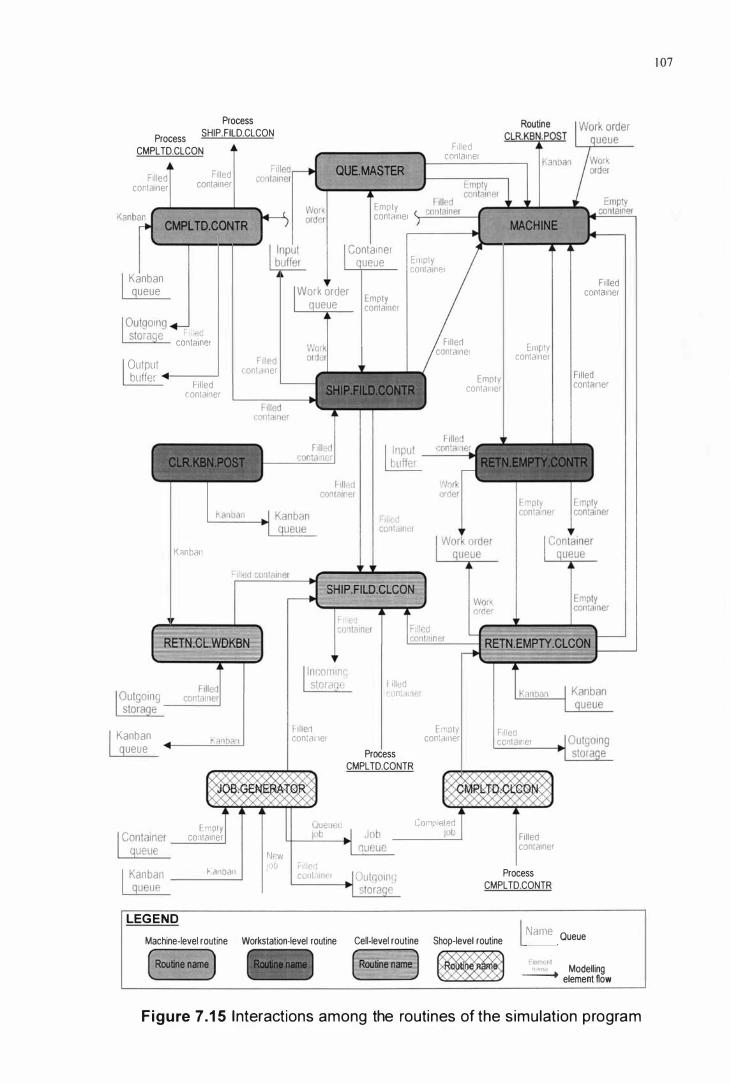
Process

Process SHIP.FlLD.CLCON

CMPLTD.CLCON

Filled container

Filled container

CMPLTO.CONTR

QUE.MASTER

Filled contamer

Empty (_...I;.....z... .... _...I���� contalnel '-.-'''''''-='''----1

Container ueue Empty

conlanlel Kanban queue Work order

ueue Empty container

F i lled contalller

r,ll .d L..:.:":'--==-:'_ cont�lnpr

Output buffer +-----'

Filled container

K�nbal'

Kanban ueue

LEG END

Empty container

I\anban

Fil led container

New

ti l led contallle,

')0 Filled contdlnPJ

Machine-level routine Workstation-Ievel routine ( Routine nana )

f ill"d r ,nt 1I'1er

Process CMPL TD.CONTR

Filled contalnel Empty

container

Empty container

E mpty contalller Filled

container

Filled contalller

Compl ted Filled container

Process CMPL TD.CONTR

Cell-level routine Shop-level routine I Name Queue

� HE!ml·rlr n •• ",;· Modelling

-----+ element flow

Figure 7.1 5 I nteractions among the routines of the simulation program

1 07

1 08

As shown in Figure 7 . 1 5 , the routines interact with each others through two ways: they

interchange modelling elements (e.g. Kanbans, fil led containers, etc . ) with the routines

they cal l , or they interact indirectly with each other through the manipulation of queues

(e.g. the input buffer).

For example, the SHIP .F ILD.CONTR process interacts directly with the MACHINE

process by passing two modell ing elements to it: the fil led container and the empty

container. On the other hand, the SHIP.FILD.CONTR process also interacts with the

MACHINE process indirectly by introducing new 'work orders' to the work order

queue. As described in 7 .2 .3 (a), work orders were used in the simulation program for

conveying the information for processing a container of parts to a specific instance of

the MACHINE process.

In this section, we have described the simulation program for the shop model. In order

to make sure that the developed program operates as we expect, it had to be verified.

The verification of the simulation program will be described in the next section.

7.3 Verification of the Simulation Model

After the simulation program was developed, all routines were successfully compiled

and the execution file for the program was generated by the compi ler. However, at this

stage, the simulation program was not yet completed. We still had to verify that the

logic and operations of the simulation program were executed as we expected.

Verification was carried out immediately after each of the four model development

stages. The fol lowing procedure was adopted to verify the simulation model :

( 1 ) Statements for issuing event messages were inserted in the program codes where

important actions took place (e.g. a container being shipped, a Kanban being

returned, a job being completed, etc . ) .

1 09

(2) Statements for detecting errors were inserted in the program codes where errors

may happen. For example, in the routine, CMPLTD.CLCON (Figure 7. 1 4),

statements were added to check whether the lot size of a container storing

completed parts was consistent with that specified by the job.

(3) The program was run with a set of test data. All event and error messages were

printed out. The size of the test data was smaller than the data for the shop

environment being model led, but sufficient for checking the actions and logic of the

program.

(4) The event messages were walked through to find any incorrect actions and logic.

All identified errors were then corrected.

I n addition, Kanbans and containers played an important role in the control of inventory

level and part movement. Therefore, after the completion of the shop-level model, the

numbers of Kanbans and containers generated were printed out and verified to assure

the routine for creating Kanbans and containers functioned correctly .

After going through the verification process, we were confident that the developed

simulation model was a correct representation of the shop environment designed in

Chapter 5 . Once the simulation model was verified, it could be executed to carry out the

experiments as designed in Chapter 6. In the next section, we will describe how to run

the simulation program to correctly col lect the statistics on the dependent variables.

7.4 Running the Simulation Program

The simulation program was executed in two phases : the prel iminary runs and the

production runs. Through prel iminary runs we determined the initial transient period,

the required numbers of conveyance Kanban-container sets and the simulation run

length (repl ications). After these parameters were determined through the preliminary

runs, production runs were performed to achieve the experiments designed in Chapter 6

and statistics on the dependent variables were collected for analysis. These tasks

1 1 0

regarding preliminary and production simulation runs wi ll be i l lustrated individually in

the fol lowing subsections.

7.4. 1 Determination of the initial transient period

I n this study, a simulation run was started from an 'empty' condition ( i .e. I nitially all

machines are idle and no job is in the system). Hence it could be expected that the

simulated system would go through a initial transient period before the dependent

variables reach a steady state . Therefore, the data gathered during the initial transient

period would have to be discarded to avoid the collected statistics being biased.

The Welch's graphical procedure (Law and Kelton 1 99 1 , p. 545) was used to determine

the initial transient period. The procedure involved the fol lowing steps:

( 1 ) Seven replications with different random number seeds of the simulation run were

made. Each replication was run for 1 30 periods, with each period being 1 20

simulated hours. Statistics on average work-in-process inventory, average flow

time and average machine uti l isation were col lected for each period, leading to

1 30 observations in each replication.

(2) Let �'i be the ith observation from the jth repl ication (j = 1 , 2, . . . , n; i = 1 , 2, . . . , m). For this study, n = 7 and m = 1 30 . To reduce the variation of the original

observations, the fol lowing averages were calculated:

- 11

X i = I Xli' In . ./= i

The above averaged process has the same transient mean curve as the original

process, but its plot has only ( l In)th the variance.

I I I

(3) To smooth out the high-frequency oscil lations in X 1 , X 2, . . . , X m (but leave the

long-run trend), the moving average X i (w) (where w is the ' window' and is a

positive integer such that w :::; [mI2] ) were calculated as fol lows :

5=-W

2 w + 1 if j = W + 1 , . . . , m - W

5=- ( i- 1 )

2; - 1 if ; = 1 , . . . , W

I n this study, w was set to 30.

(4) X i (w) for i = 1 , 2, . . . , m-w was plotted and a value of i = I was chosen so that

X l+ l (W) , X 1+2(W) , . . . appeared to converge.

From the results of prel iminary runs, we found that the cel lular layout shop with single­

unit production & conveyance and backtracking flow allowed ( i .e . the CSB shop) had

the longest average flow times. Therefore, the initial transient period was determined

based on the moving averages of the dependent variables for the CSB shop since it took

the longest time to reach a steady state. The resulting moving average plot of average

work-in-process inventory for the CSB shop was shown in Figure 7. 1 6 . (The moving

average plots for the three dependent variables are presented in Figures A6. 1 -3 of

Appendix 6). The moving averages appeared to converge after the 48th period.

Therefore, we decided to set the initial transient period, 1 = 48 periods = 5760 hours.

200

t 1 50 '" 0..

'+-< � 100 Cl)

.D E Z 50

o

L _ Period ( 1 20 hrs )

Figure 7 . 1 6 Moving average plot of average work-in-process inventory

(Cel lu lar layout with SUPC and backtracking flow al lowed)

7.4.2 Determination of the numbers of conveyance Kanban-container sets

1 1 2

I n a production system with Kanban-based production control, the numbers of

conveyance Kanbans and containers (used as production Kanbans in this study)

designated for each part type at each workstation are critical for the control of

inventory-level and part movement.

The numbers of Kanbans and containers were set in pairs. A container for storing the

parts for a specific part type at a workstation was assigned an associated conveyance

Kanban for authorising the movement of this container. I f the numbers of Kanban /

container sets (for individual part types) were set too small , the production flow would

be too tight ( i .e. be blocked too often) because the numbers of Kanban-container sets

were not enough for circulating parts smoothly. On the other hand, if the numbers of

Kanban-container sets were too large, the production flow would be too loose because

parts would be routed through machines faster at the cost of higher work-in-process

inventory.

1 1 3

In a shop environment where production flow was too tight or too loose, the effects of

independent variables on the responses of dependent variables can be biased. For

example, if the production flow is too tight, a large setup time reduction may result in

significantly less or no improvement in average flow time because of the blockage of

the production flow. Consequently, in order to assess the shop performance corre·ctly,

reasonable numbers of Kanban-container sets need to be determined. I n this study, the

simulation approach presented by Phil ipoom et al. ( 1 987) was used to determine the

required numbers of Kanban-container sets through prel iminary simulation runs.

The fol lowing steps were involved for determining the numbers of Kanban-container

sets required for individual part types among the workstations in a cel l :

( 1 ) A simulation run was made for each workstation assummg that the production

system was operated without backorder. In other words, when a fil led container

arrived at a workstation, there was always an available corresponding empty

container for initiating the processing of the filled container. This assumption

enabled all workstations to be 'decoupled' from each other.

(2) The production lead times of Kanban lots (batches) for each part type at a

workstation were recorded for every 1 1 th arrival so that the dependence among

observations were reduced.

(3) 1 00 observations were collected m this manner for each part type at each

workstation. These 1 00 lead time observations were ranked from smallest to largest

and the 95th highest value was used as the estimated lead time value (denoted by

L T9S)·

(4) The fol lowing formula was used to determine the number of conveyance Kanban /

container sets required for a specific part type at a workstation:

n = D x L T9S (7. 1 )

1 1 4

where n is the number of conveyance Kanban-container sets required for a part type

at a workstation. D is the average demand of the part type in containers ( lots) per

day. LT95 is the estimated lead time value for the part type at the workstation in days.

(5) In addition to equation (7. 1 ), the fol lowing constraint has to be satisfied for the

cellular layout shops with single-unit production and conveyance (Yavuz and Satir

1 995) :

n "2 LS (7.2)

where LS is the order lot size for a specific part type. For a cellular layout shop with

single-unit production and conveyance (SUPC), the Kanban lot size for intra-cel l

part movement was one. Therefore, if the number of intra-cel l Kanbans was set to be

less than the order lot size, the workstation would starve for input material during

the processing of a container (batch) of parts, and the system would be blocked.

As an example, Table 7 .5 shows the numbers of intra-cell conveyance Kanbans for cell

1 of the cellular layout shop with batch production & conveyance (BPC) and

unidirectional flow (i .e . the CBU shop). For example, for part type 6, the required

number of Kanbans at workstation 3 (of machine type 1 0) was one. It means that one

conveyance Kanban-container set was required for transporting the parts for part type 6

from workstation 2 to workstation 3 . Similarly, one conveyance Kanban-container set

was required for the part movement of part type 6 between workstation 3 and

workstation 4.

Note that workstation 2 was the first workstation in cell 1 on the routing for part type 6.

Therefore, the required number of Kanbans at workstation 2 indicates the available

number of input buffer spaces for storing fil led containers moved from the cell

incoming storage.

l i S

Table 7.5 N umbers of intra-cel l Kanbans for cell 1 of the CBU shop

Part Demand Number of Kanbans at Type ( lots/day) Workstation No.lMachine type

1 /1 2/6 3/1 0 4/7 5/9

5 1 .85 1 2 1 1 1

6 1 . 39 1 1 1

1 1 0 .95 1

1 5 0 .50 1 1

1 6 0.62 1 1

The required numbers of conveyance Kanban-container sets for inter-cell part

movement were determined in the same manner by assuming there was no backorders

among cells . The same procedure as described above was followed to determine the

required numbers of conveyance Kanban-container sets for inter-cel l part movement. In

this case, LT95 is the estimated lead time value for a specific part type at a cell in days.

As an example, Table 7.6 shows the required numbers of inter-cel l Kanbans for the

cellular layout shops with unidirectional flow. For example, for part type 6, the required

number of conveyance Kanban-container sets at cel l 2 was two. In other words, two

conveyance Kanban-container sets were required for transporting the parts of part type 6

from cell 1 to cell 2 . Since cell 1 was the first cell on the routing for part type 6, the

requirement of two Kanbans at cell I indicates two conveyance Kanban-container sets

were required for transporting the parts for part type 6 from the receiving department to

cell 1 .

The required numbers of intra-cel l and inter-cel l conveyance Kanban-container sets for

individual part types were given in Appendix 7. Since the shop configurations for the

cellular layout shops with backtracking flow and those with unidirectional flow were

different, a set of figures were obtained for each of the two basic shop layouts.

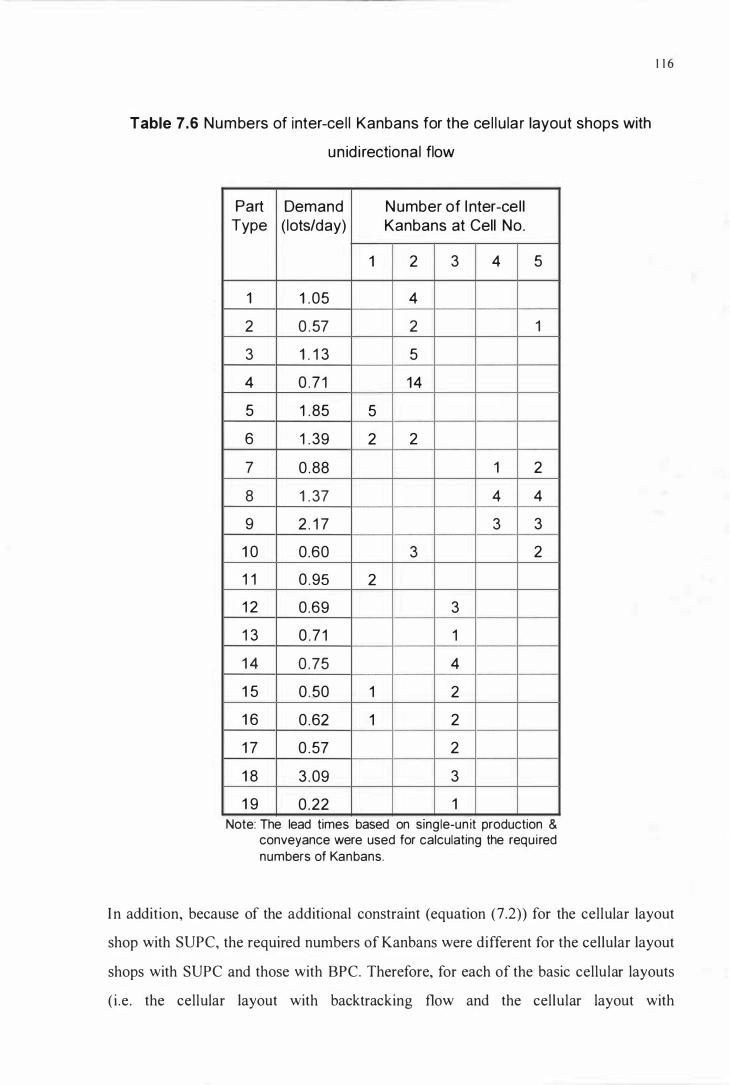
Table 7.6 Numbers of inter-cel l Kanbans for the cel lu lar layout shops with

un id i rectional flow

Part Demand Number of I nter-cel l Type (lots/day) Kanbans at Cell No.

1 2 3 4 5

1 1 .05 4

2 0 .57 2 1

3 1 . 1 3 5

4 0 .71 14

5 1 . 85 5

6 1 . 39 2 2

7 0 .88 1 2

8 1 . 37 4 4

9 2 . 1 7 3 3

1 0 0.60 3 2

1 1 0 .95 2

1 2 0.69 3

1 3 0 .7 1 1

1 4 0 .75 4

1 5 0 ._50 1 2

1 6 0 .62 1 2

1 7 0 .57 2

1 8 3 .09 3

1 9 0 .22 1 Note: The lead times based on single-unit production &

conveyance were used for calculating the required numbers of Kanbans.

1 1 6

I n addition, because of the additional constraint (equation (7.2)) for the cellular layout

shop with SUPC, the required numbers of Kanbans were different for the cellular layout

shops with SUPC and those with BPC. Therefore, for each of the basic cellular layouts

( i .e . the cellular layout with backtracking flow and the cellular layout with

1 1 7

unidirectional flow), the required numbers of Kanbans for SUPC and BPC were

obtained individual ly.

7 .4 .3 Determination of the simulation run length (replications)

As i l lustrated in Subsection 7.4. 1 , in each simulation run, the system would go through

a initial transient period before the dependent variables reach a steady state. At the end

of the transient period, statistics on dependent variables were reset and independent

observations of the statistics on the dependent variables could be col lected. I n this study,

an observation was defined as the statistics (e.g. average) col lected for a specific

dependent variable during a period in the simulation run.

For a simulation model with stochastic characteristics, a simulation run has to be

replicated (to collect more than one observations) to achieve the desired accuracy for the

statistics on dependent variables. Although higher accuracy can be achieved through

more replications, computing time also increases with increasing replications. Therefore,

to perform simulation efficiently, it is important to decide the replications (or simulation

run length) required for calculating statistics with the desired accuracy.

In this study, the blocking method (Emshoff and Sisson 1 970: 1 99-200) was employed

for collecting observations of the statistics on the dependent variables. However, we had

modified thi s primitive method to reduce the degree of correlation among observations.

Through several preliminary simulation runs, we decided to collect observations of the

statistics on the dependent variables for every 1 200-hour data-recording period. To

assure the independence of observations ( i .e . to reduce the auto-correlation), a 520-hour

non-recording period was introduced between any two adjacent data-recording periods

to ensure that jobs entering the system in the previous period were completed before the

start of the next period. Statistics on dependent variables were reset at the beginning of

each data-recording period.

1 1 8

By using the method a/batch means presented by Law and Kelton ( 1 99 1 : 554-555), the

sample mean and variance (as estimators for the population mean, � and variance, 'f/,

respectively) of a dependent variable in a simulation run were given as fol lows:

11 _

Y (n, k) = I Y j (k) j n j= i

n _

S(n) = I [ Yj (k) - Y (n, k)]2 j (n- l ) j=i

where

k = data-recording period = 1 200 hours

(7. 1 )

(7.2)

n = total number of data-recording periods (replications) of the simulation run.

Y (n, k) = sample mean of the dependent variable, Y for the simulation run with n

data-recording periods of length k.

Y /k) = sample mean of the dependent variable, Y in the jth data-recording period.

S (n) = sample variance of the dependent variable, Y for the simulation run

The estimate of the 1 00( l -a) percent confidence interval for the population mean � of

the dependent variable, Y is given by

= [S2W Y (n, k) ± In- I , l -a/2 �--;;- (7.3)

where In- I , l -a/2 is the upper I -a/2 critical point for the t distribution with n- l degrees of

freedom. Formula (7 .3) shows that as the number of replications ( i .e. n) increases, the

error term ( i .e . '"- I . 1 -(112 � 5' ; n ) ) for estimating the population mean decreases.

From the preliminary simulation runs, we found that with twenty-two replications (i .e . n

= 22), errors equal to or smaller than 1 0% could be achieved for estimating the

1 1 9

population means with a 95% confidence interval . Therefore, we decided that

observations of the statistics for the three dependent variables were gathered for twenty­

two data-recording periods (i .e . twenty-two replications) in a simulation run, leading to

twenty-two independent observations.

7.4.4 Performing the production simulation runs

After the initial transient period, the required numbers of Kanbans and the number of

replications had been decided, the simulation experiments were then carried out through

production simulation runs. Each production simulation run was performed with a set of

data representing a different combination of the levels for the independent variables.

The levels of the independent variables to be investigated have been summarised in

Table 6. 1 of Section 6. 1 .

F or example, as shown in Table 6 . 1 , the shop configuration with the SL level = FL, the

PFSRF level = 0.7 and the low inter-department material handling speed setting ( i .e.

with the MHS level = LLL, LLH or LHH) was simulated in one production simulation

run. Therefore, in total 54 production simulation runs (six for the SL level = FL and

twelve for each of the other four SL levels) were performed for the first set of

experiments. Observations of the statistics on the three dependent variables were

collected in each simulation production run as described in the last subsection. The

results of the simulation experiments was then analysed by using the methods presented

in Section 6 .3 .

In this chapter, we have i l lustrated the development and operation of the simulation

model for the first set of experiments. The developed simulation model possessed all the

required functions for the experimental system as presented in Chapter 5 . Furthermore,

we determined several essential parameters for running the simulation model, such as

the initial transient period, the numbers of conveyance Kanban-container sets and the

simulation run length (replications). In the next chapter, we will present the analyses

and discussions of the simulation results for this set of experiments.

CHAPTER 8

ANALYSES AND DISCUSSIONS OF THE SIMULATION RESULTS FOR

THE FIRST SET OF EXPERIMENTS

1 20

This chapter presents the results and discussions of the simulation output and statistical

output analyses for the first set of experiments. As i l lustrated in Subsection 5 .5 . 1 , to

have fair comparisons among the shops with different layouts and production flow

patterns, the total numbers of parts produced for individual part types ( i .e. the demands

for individual part types) were the same for all shops investigated at each level of the

Part Family Setup Reduction Factor (PFSRF). Therefore, to compare the different shops

on the same basis, the results were also presented and discussed for each of the high,

medium and low levels of the PFSRF variable separately. However, the influence of the

Part Family Setup Reduction Factor sti l l can be examined by comparing the results

across the three PFSRF levels.

8.1 Simulation Results and Discussions for the High PFSRF Level

At each of the Part Family Setup Reduction Factor levels the simulation output was

analysed in two ways. First, the graphical method was used. The differences in the

performances of individual shops were examined by presenting the simulation output in

bar charts. Next, the hypotheses proposed in Section 6.3 were tested, and results and

discussions were presented. By using the two analysis methods, the maximum

information can be extracted from the simulation output.

8 . 1 . 1 Discussions of the simulation output presented in bar charts

The sample mean values on the three dependent variables, average work-in-process

inventory (A WIP), average flow time (AFT) and average setup to processing time ratio

(ASPTR) from the first set of experiments at the high PFSRF level are presented in

Figure 8 . 1 .

1 80

1 60

r:::- 140 e 11 1 20 u. 0::: 1 00 (j) u. 80 e:-

a.. 60

� 40 <t:

20

1 I r I - � -re >-1 Ii' ,.. tf - 1 , rr � -I I - .E

I '" i'" ' . f'" f" I l · - l --

-

0 LLL LLH LHH HLL HLH

Level of MHS

* The error l ines indicate the 95% confidence intervals for J1. .

30

25 r:::-

- - -=t

e 20 1 1 i U. 0::: (j) 1 5

1 1 , u.

e:- 1 0 I-u. .... 'Cb r" "'" <t: 5 ,

0 LLL LLH

L

4,5

4,0 r:::-

3,5 e -

P-, 11 3,0 u. I -

0::: (j) 2.5 u. t'-- , :'" -

e:- 2,0 C= �

0::: 1 .5 I- I a.. 1 ,0 (j) r <t: 0,5

0,0 LLL LLH

r ]1

I f

I I

� I I I I

-:-

I 1

� r"--=r' I r"""i"'"

,...

I LHH HLL

Level of MHS

-

� , t

r 1"" -F

� LHH HLL

Level of MHS

-

1 I

F- ,..,

I , HLH

for] I ,

-, I I

I HLH

'f-It --

-

I- :'" f"

� I

HHH

1>- -

f-- -

I r-= I-

HHH

-

"1-I -

fb-f r

f t

HHH

tt

le-I '-I

r

"l r I ,-

'-

I � I

i-FL� I · CBB o CBU . CSB

I[J C� I

-- I 11 FL

I . CBB I j CBU I

I . CSB I 1 ::J CSU I

-,

r. FL I . CBB I CBU I t . CSB I

I' �suj l

Figure 8 . 1 Simu lation output summary of the first set o f experiments at

PFSRF level = High

1 2 1

1 22

For each dependent variable, the sample mean values in bar charts for the individual

levels of the Shop Layout independent variable (i .e. FL, CBB, CBU, CSB and CSU) are

presented for each level of the Material Handling Speed (MHS) independent variable.

(See Section 6 . 1 for the definition of the independent variable levels). The error l ines on

the bar graphs represent the ranges of 95% confidence intervals for the population

means of the dependent variables.

Apparently, at this level of the Part Family Setup Reduction Factor, the performances of

the cellular layout shops with single-unit production and conveyance (SUPC) (i .e. CSB

and CSU shops) were substantial ly inferior to those of other shops, even if the intra-cell

material handling speed was fast (at the LLH, LHH, HLH and HHH levels of MHS).

This outcome was contradictory to the long held view of several lIT proponents (Cheng

and Podolsky 1 993; Monden 1 983 ; Schonberger 1 986; Shingo 1 989) that SUPC is

essential for eliminating delay by lot conveyance and increasing production lead time. I t

seems that the argument does not always hold true in a job shop environment.

In a repetitive manufacturing environment, where job routings and setup times are more

uniform, the benefits of single-unit production and conveyance can be achieved more

easily because parts can be routed through workstations one piece by one piece

smoothly without build-up of queues between operations. However, in a job shop

environment, since routings of jobs are more variable, pieces of parts from different jobs

may arrive at the input buffer of a workstation in the same period. Consequently, pieces

of parts belonging to the same job may not be processed continuously by a workstation.

In other words, delay times wil l be introduced between the operations of a part.

We wil l give an example here to explain the delay between the operations of a part. For

the cellular layout with backtracking flow allowed, both part types 1 and 1 0 were

processed by cell 2 . The sequences of machine types required for processing part types

1 and 1 0 are 1 -4-8-9 and 4-7-4-8 , respectively. We assume that a batch ( lot) of part type

1 is being processed by machine type 1 . Now one piece of part type 1 is completed on

machine type 1 and moved immediately to machine type 4 for another operation. At this

1 23

time, a batch of part type 1 0 arrives and it is queued in front of machine type 4 since the

operation on the piece of part type 1 is going on. If the operation on the piece of part

type 1 on machine 4 is completed before the next piece of part type 1 comes, machine

type 4 will now be setup for processing the batch of part type 1 0 since it is the first in

the queue. Once machine type 4 starts processing the batch of part type 1 0, it will not be

switched to processing other part types unti l the whole batch is completed. Therefore, if

a piece of part type 1 arrives at machine type 4 when the batch of part type 1 0 is being

processed, it has to wait until the completion of the batch of part type 1 0 . As a result, a

period of time delay (while waiting for the completion of the batch of part type 1 0) will

be incurred between this piece and the previous piece of part type 1 . S imilarly the same

situation may happen for machine type 8 since it is required by both part types 1 and 1 0.

This finding about the delay between operations for job shop manufacturing is

consistent with that reported by Kelleher ( 1 986), who claimed that to attain the benefits

of single-unit production and conveyance, there is a need to keep the operations

balanced (synchronised) to avoid queues between operations.

Less synchronised operations led to two major drawbacks. First because machine setups

happened more often to switch the production between different part types (e.g. part

types 1 and 1 0 in the above example), the time spent for setting up machines (or average

setup to processing time ratio) became higher. Consequently, the benefit of setup time

reduction brought about by cellular manufacturing was offset by the higher setup time.

Second, the advantage of eliminating the delay caused by lot conveyance (See Section

1 .2) by adopting single-unit production and conveyance was also offset by the delay

between operations. Eventually, the potential of single-unit production and conveyance

in reducing flow time might not be real ised.

With the high PFSRF level, the effect of unsynchronisation between operations was

more severe because parts had to spend longer times waiting for machine setups and

thus pieces of parts from different jobs were more l ikely to be queued in front of

workstations. Furthermore, because workstations / cells are closely l inked to each other

1 24

through Kanban signals in a Kanban-based system, any fluctuation in part of the system

can be easily transmitted (and even amplified) to the entire system (Kimura and Terada

1 98 1 , Vi l leda et al. 1 988) . Therefore, the highly unsynchronised operations caused by

single-unit production and conveyance rendered the Kanban-control led job shop

unstable and eventually led to its poor performance.

Figure 8 . 1 shows that the influence of material handl ing speed on the individual

performances of the cel lular layout shops with single-unit production and conveyance

(i .e . CSB and CSU) were not significant. Though it seemed that average work-in­

process i nventory or average flow time was lower at some material handl ing speed

levels for the two shops, we are not confident of these differences since there were

always overlaps for their 95% confidence intervals of means at different MHS levels.

For the cellular layout shops with single-unit production and conveyance, the shop with

unidirectional flow (i .e . the CSU shop) had lower average setup to processing time ratio

than that with backtracking flow allowed ( i .e . the CSB shop) at all the MHS levels. The

unidirectional flow seemed to be effective in alleviating the adverse effect of

unsynchronised operations. However, the differences in the A WIP and AFT

performances of the CSB and CSU shops were not as significant as for their ASPTR

because there were always overlaps among the 95% confidence intervals of their A WIP

and AFT.

As shown in Figure 8 . 1 , the cellular layout shops with batch production and conveyance

(i .e . the CBB and CBU shops) had significantly lower average setup to processing time

ratios than those of the functional layout (FL) shop. The superior performance of the

CBB and CBU shops on ASPTR, however, did not result in better performance on

average work-in-process inventory and average flow time. This finding wil l further

discussed in the next subsection

No significant effect of material handl ing speed on the individual performances of the

FL, CBB and CBU shops can be identified.

8 . 1 .2 Discussions of the results of overal l F-tests and planned comparisons

1 25

The bar charts given in Figure 8 . 1 were most useful for identifying the differences in the

performances of individual shops over the different Material Handling Speed levels (e.g.

We can easily see that the mean values on A WIP for the CSU shop are lower at the LLL

and HLL levels of MHS) . However, the use of bar charts in comparing the performances

of different shops, particularly for the comparison between groups of shops (e.g.

comparing the functional layout shop with all the cellular layout shops), was limited.

Overall F-tests and planned comparIsons were more powerful for comparmg the

performances between different shops. The differences in the performances among

different shops could be identified more precisely with a specific level of significance.

In addition, planned comparisons were particularly useful for comparing groups of

shops.

Table 8 . 1 shows the sample means, sample variances and 95% confidence intervals of

population means for average work-in-process inventory at the high level of the Part

Family Setup Reduction Factor. Apparently, the performances of the cellular layout

shops with single-unit production and conveyance ( i .e. CSB and CSU shops) were

highly variable ( i .e . with very large variances) and very inferior to those of other shops

( The output summary of the al l three dependent variables are given in Tables A8 . 1 -3 of

Appendix 8 ) .

The F values calculated with such large differences in variances wil l be significantly

biased although the F-test is robust to the assumption of equality of variances.

Furthermore, although the approximate F test used for the planned comparisons is able

to take into account unequal variances, many degrees of freedom will be lost and the

power of tests will be much lower with greatly different variances. Hence, we decided

that data for the cellular layout with single-unit production and conveyance (i .e. CSB

and CSU) were not to be included in the overall F-test and planned comparisons.

1 26

Table 8 . 1 Simulation output summary on AWI P for the first set of experiments

at the high PFSRF level

Dependent MHS SL Sample 95% confidence Sample variable level level size interval for J.1 variance

FL 22 58.38 ± 1 .28 8.35 eBB 22 61 .98 ± 2 .01 20.50

LLL eBU 22 63.92 ± 1 .99 20.20

CSB 22 143.84 ± 1 3.99 995.08 CSU 22 1 23.50 ± 1 2.03 736.20

FL 22 58 .38 ± 1 .28 8.35 eBB 22 6 1 .98 ± 2 .01 20.50

LLH eBU 22 63.92 ± 1 . 99 20.20 CSB 22 149. 1 8 ± 1 4.97 1 1 40.28 CSU 22 1 32.28 ± 1 3.27 895.94 FL 22 58.38 ± 1 . 28 8.35

Average work·in- eBB 22 60.74 ± 2. 1 1 22.54 process LHH eBU 22 62. 88 ± 1 . 77 1 5.99 inventory CSB 22 1 49. 1 8 ± 1 4.97 1 1 40.28 (AWIP) CSU 22 1 32.28 ± 1 3.27 895.94

FL 22 58 . 1 1 ± 1 . 36 9.39 eBB 22 6 1 .60 ± 2. 1 0 22.33

HLL eBU 22 63.81 ± 1 . 77 1 5.98 CSB 22 1 36.92 ± 1 0. 1 4 523.04 CSU 22 1 24.68 ± 1 2.54 799.44 FL 22 58. 1 1 ± 1 . 36 9.39

eBB 22 6 1 .60 ± 2. 1 0 22.33 HLH eBU 22 63.81 ± 1 .77 1 5.98

eSB 22 1 45.09 ± 1 2.79 832.44 CSU 22 1 29.72 ± 1 1 .9 1 72 1 .6 1 FL 22 58 . 1 1 ± 1 . 36 9.39

eBB 22 60.63 ± 1 . 96 1 9.49 HHH eBU 22 62.73 ± 1 .89 1 8.24

CSB 22 1 45.09 ± 1 2.79 832.44 CSU 22 1 29.72 ± 1 1 .9 1 72 1 .6 1

Since the data for CSB and CSU shops were not included in the planned comparisons,

the two null hypotheses :

Ho( l b) : �CSB = �csu and

Ho(2) : �CBB + �CBU = �CSB + �CSU

were not tested. Ho(3) was then reduced to

Ho(3) : �FL = 1 /2( �CBB + �CBU)'

1 27

Significant overal l differences among the levels of Shop Layout were detected via the

overall F-tests on all dependent variables for all MHS levels at a significance level of

0 .002 or lower (See Table A9. 1 of Appendix 9) . Table 8 .2 summarises the results of the

planned comparisons (Refer to Table A l 0 . 1 -3 of Appendix 1 0 for detai ls). The results

of the hypothesis tests are discussed individually as follows.

Table 8.2 Resu lts of planned comparisons for the first set of experiments

at the h igh PFSRF level

Dependent MHS Ho( 1 a) Ho(3)

variable level

LLL CBB=CBU FL « CBB+CBU)/2

LLH CBB=CBU FL « CBB+CBU)/2

AWI P LHH CBB=CBU FL « CBB+CBU)/2

HLL CBB=CBU FL « CBB+CBU)/2

HLH CBB=CBU FL « CBB+CBU)/2

H H H CBB=CBU FL « CBB+CBU)/2

LLL CBB=CBU FL « CBB+CBU)/2

LLH CBB=CBU FL « CBB+CBU)/2

AFT LHH CBB<CBU FL « CBB+CBU)/2

HLL CBB<CBU FL « CBB+CBU)/2

HLH CBB<CBU FL « CBB+CBU)/2

HHH CBB<CBU FL « CBB+CBU)/2

LLL CBB=CBU FL>(CBB+CBU)/2

LLH CBB=CBU FL>(CBB+CBU)/2

ASPTR LHH CBB<CBU FL>(CBB+CBU)/2

HLL CBB<CBU FL>(CBB+CBU)/2

HLH CBB<CBU FL>(CBB+CBU)/2

HHH CBB<CBU FL>(CBB+CBU)/2

Note: For al l significant differences, p :-:; 0.05.

1 28

(a) Comparison between the two cel lular layout shops with batch production and

conveyance [by testing Ho( 1 a)]

Between the cellular layout shops with batch production and conveyance (BPC), the

shop with backtracking flow allowed (i .e . CBB shop) and the shop with unidirectional

flow (i .e . CBU shop) performed equally in terms of average work-in-process inventory.

But the CBB shop was superior to the CBU shop on the other two dependent variables

when the intra-cell batch flow or inter-cel l part movement speed was at the high setting.

The findings show that more efficient intra-cell material handling did make the shop

with backtracking flow al lowed superior to the shop with unidirectional flow for the

cellular layout with batch production and conveyance at the high PFSRF level .

On the other hand, SInce the CBU shop had been designed to achieve intra-cell

unidirectional flow by creating inter-cell flows wherever necessary, it seems that more

efficient i nter-cell material handling should make the CBU shop perform better.

However, with high PFSRF, even though parts were transported quickly from preceding

cells to succeeding cells, they sti l l had to spend a lot of time waiting for machine setups

because of the higher setup times. Consequently, jobs were more likely to be congested

at succeeding workstations with a high inter-cell material handling speed setting. This

effect resulted in higher average setup to processing time ratio, which in turn led to

higher average flow time.

(b) Comparison between the functional layout and the cellular layouts [by testing Ho(3 )]

The comparison between the functional layout ( i .e. FL) and the cel lular layouts ( i .e .

CBB and CBU) through Ho(3) shows that the shops with cellular layout consistently

demonstrated lower average setup to processing time ratio than that of the shop with

functional layout. This outcome is expected since the cellular layout was designed to

capitalise on the similarities among the operational sequences of parts produced to

achieve setup time reduction. However, despite their superior performance on ASPTR,

the performance of the cellular layout shops on A WIP and AFT was inferior to that of

the functional layout shop.

1 29

Flynn and Jacobs ( 1 987) reported that though cellular manufacturing is effective in

reducing setup times, a certain degree of inflexibil ity is also caused by dedicating

machines in a cell to the production of a specific fami ly of parts. In the functional layout,

when a job arrives at a department with interchangeable machines of the same type, it

can be processed on any machine that is avai lable. However, in the cellular layout, a

machine is only permitted to process parts of the fami ly assigned to it . The consequence

of the inflexibility of cellular layout is that machines tend to be less uti l i sed (Morris and

Tersine 1 990) and build-up of queues is l ikely to happen. When the Part Family Setup

Reduction Factor was high, the effect of inflexible use of machines was prominent for

the cellular layout and led to poor queue-related performance, such as average work-in­

process inventory. Eventual ly, the benefit of reduced setup times brought about by

cellular manufacturing was more than offset by its poor A WIP performance at the high

PFSRF level . Unavoidably, inferior performance on average work-in-process inventory,

in turn, led to the inferior performance of average flow time.

The findings in this section show that functional layout should be more suitable for a

job shop environment with Kanbans when the extent of setup time reduction achievable

through cellular manufacturing is small ( i .e . at the high level of the Part Fami ly Setup

Reduction Factor).

It is useful to note that the (statistical ly) significant differences identified by the planned

comparisons seem not so important (in practice) on the bar charts in Figure 8 . 1 . Those

small differences could be identified statistically because the degrees of freedom for the

planned comparisons were large enough.

Though statistical significance may not be scientifical ly important, it does provide

important guidelines for industrial applications. For example, in Subsection 8 . 1 .2, the

results of planned comparisons show that the functional layout (FL) was superior to the

cellular layouts (eBB and eBU) though the differences were not very important on the

bar charts. Knowing this finding, engineers who are designing Kanban systems in job

shop environments may want to conduct further experiments (with real or simulated

1 30

systems), which incorporate the actual shop conditions and configurations, to assess the

differences among these layouts.

I n addition, it is not l ikely that the conditions in real manufacturing shops are as well

control led as those in simulated shop environments. If the similar experiments are

performed in real shop environments, the dependent variables may be affected not only

by the levels of the independent variables, but also by other uncontrol led factors.

Therefore, differences that may not appear to be practical ly important in simulation

experiments may turn out to be important in real shop environments. Besides, for a wel l

managed shop where production goes smoothly, sometimes even small amounts of

improvement are critical for remaining competitive in the market.

The results and analyses of the simulation output for the medium level of the Part

Family Setup Reduction Factor will be discussed in the next section.

8.2 Simulation Results and Discussions for the Medium PFSRF Level

The discussions in this section are also in two parts. First, bar charts are used to examine

the differences in the performances of individual shops. Next, the results from the

overall F-tests and planned comparisons are presented and discussed.

8 .2 . 1 Discussions of the simulation output presented in bar charts

Figure 8 .2 shows the sample means and the 95% confidence intervals of population

means for the dependent variables at the medium level of PFSRF. Again, material

handling speed did not have any significant effect on the individual performances of the

various layouts. However, one significant change at this level of the Part Fami ly Setup

Reduction Factor is that between the two cellular layout shops with single-unit

production and conveyance ( i .e . CSU and CSB shops), the CSU shop outperformed the

CSB shop on all dependent variables. We are confident of the differences since there is

no overlap between their 95% confidence intervals of population means.

1 40

1 20 LO 0 1 00 - -11 U. a:: 80 -Cl) u.

60 e:- "'-F a... 40 � « 20

0 LLL

1 8

1 6

LO 1 4 -0 1 2 1 1 --u.

1 0 a:: -Cl) u. 8 "" �

e:- 6 I-u. 4 «

2

0 LLL

3.0

LO 2.5 0 1 1

2.0 u. -a:: Cl) u. 1 .5 e:- .... a:: 1 .0 I-a... Cl) 0.5 «

0.0 LLL

g, - -

_El' "-

-

'f

f-

LLH

11 r '.:l:; .

I

LLH

Il �

LLH

� >-I "'"

�l I Fa.

!

I .

, I

r-I I

l I ,

�

'3 � -,-.. -' - -

I'" � r= ,.... I-

I � t - I

LHH HLL

Lel.€i of MHS

� ; - R I � -- I I I I -

, LHH HLL

Lel.€i of MHS

,. 1=, I f r"

� r-

I LHH HLL

Lel.€i of MHS

1 - r

- -r'" 1-- '" I f-f-

HLH

- ,

tb-�

"" -� I -f --

r-HLH

-"

.. -, L

- .-

I-

I"

HLH

--

- a -

...

HHH

.:r -

-- It

j-

r I HHH

1--,

r r ,-

� r HHH

r;FL I I · CBB I o CBU

I . CSB I I [ CSU l _ I

III FL 1 1 I . CBB I I CBu l . CSB I r CSU I

�- I FL I . CBB I o CBU . CSB I I [ CSU

Figure 8.2 Simulation output summary of the first set of experiments

at PFSRF level = Medium

1 3 1

1 32

This finding supports the discussion in the previous section and shows that the cellular

layout shop with single-unit production and conveyance was more susceptible to the

degree of synchronisation of production flow than other shops. When parts flowed in

the same forward direction in a cell, production flows tended to be smoother and more

synchronised than with backtracking flow allowed. Therefore, unidirectional flow was

effective in alleviating the adverse effect of unsynchronised operations on the shop

performance caused by single-unit production and conveyance.

8.2.2 Discussions of the results of overall F-tests and planned comparisons

Overall F-tests and planned comparisons were performed to identify the differences in

shop performances caused by the different levels of the Shop Layout variable. Table 8.3

shows the sample means, sample variances and 95% confidence intervals of population

means for average work-in-process inventory at the medium level of the Part Family

Setup Reduction Factor. For the cellular layout shops with single-unit production and

conveyance, the sample variances of the shop with unidirectional flow (i .e . the CSU

shop) were relatively much smaller than at the high level of PFSRF, but the sample

variances of the shop with backtracking flow allowed ( i .e. the CSB shop) were sti l l

large. For the same reason as stated in Subsection 8. 1 .2, the data for the CSB shop were

not included in the overall F-tests and planned comparisons to provide more power for

the hypothesis tests (The output summary of the all three dependent variables are given

in Tables A8 .4-6 of Appendix 8) .

Therefore, Ho( 1 b) was not tested because the data for the CSB shop were not included.

Ho(2) was then reduced to:

Ho(2) : 1 /2(/-!cBB + /-!CBU) = /-!CSU.

If Ho(2) was true, no difference could be identified among the performances of cellular

layout shops, and Ho(3) would be reduced to

Ho(3) : /-!FL = 1 /3 ( /-!CBB + /-!CBU + /-!csu) ·

1 33

Table 8.3 Simu lation output summary on AWI P for the first set of experiments

at the medium PFSRF level

Dependent MHS SL Sample 95% confidence Sample variable level level size interval for J.l variance

FL 22 63.90 ± 1 .97 1 9.69 eBB 22 62.23 ± 1 . 56 1 2 .42

LLL eBU 22 62. 14 ± 1 .31 CSB 22 1 1 1 .28 ± 8.07 esu 22 87.20 ± 4 .30 FL 22 63.90 ± 1 . 97 1 9.69

eBB 22 62.23 ± 1 .56 1 2 .42 LLH eBU 22 62. 1 4 ± 1 . 31 8 .76

eSB 22 1 1 2. 1 7 ± 8.27 347.87 esu 22 92.46 ± 5.40 1 48.06

FL 22 63.90 ± 1 . 97 1 9.69 Average work·in· eBB 22 60.67 ± 1 .68 1 4.33 process LHH eBU 22 60. 71 ± 1 .40 9.93 inventory CSB 22 1 1 2.77 ± 8.27 347.87 (AWIP) esu 22 92 .46 ± 5.40 1 48.06

FL 22 63.62 ± 1 . 74 1 5 .42 eBB 22 61 .30 ± 1 .55 1 2. 1 7

HLL eBU 22 62 .81 ± 1 .38 9.72 CSB 22 1 1 1 .53 ± 8.06 330.68 esu 22 88.98 ± 4.42 99.43 FL 22 63.62 ± 1 . 74 1 5.42

eBB 22 61 .30 ± 1 .55 1 2. 1 7 HLH eBU 22 62 .8 1 ± 1 . 38 9.72

eSB 22 1 1 6.46 ± 9.91 499. 1 1 esu 22 91 .89 ± 5.72 1 66.57 FL 22 63.62 ± 1 . 74 1 5.42

eBB 22 60.20 ± 1 .65 1 3.90 HHH eBU 22 61 .22 ± 1 .39 9.82

eSB 22 1 1 6.46 ± 9.91 499. 1 1 esu 22 91 .89 ± 5.72 1 66.57

I f Ho(2) was rejected, the functional layout would be compared with the cellular layout(s)

with superior performance. Therefore, Ho(3 ) would be reduced to

Ho(3) : J...I.FL = 1 /2( J...I.CBB + J...I.CBU )

if the cellular layout shops with batch production and conveyance (i.e. the eBB and

eBU shops) were found to be superior, or be reduced to

Ho(3) : J...I.FL = J...I.csu

1 34

if the cellular layout shop with single-unit production and conveyance (i .e . the CSU

shop only) was found to be superior.

The overall differences among the levels of the Shop Layout variable on all dependent

variables were found to be significant by the overall F-tests for all MHS levels at

significance levels lower than 0.00 1 (Refer to Table A9.2 of Appendix 9 for details).

The results of planned comparisons are presented in Table 8.4 (Refer to Tables A 1 0.4-6

of Appendix 1 0 for details). The results of the hypothesis tests are discussed

individually below.

(a) Comparison between the two cellular layout shops with batch production and

conveyance [by testing Ho( 1 a)]

The results of the comparison between the cellular layout shops with batch production

and conveyance show almost the same patterns as for the high PFSRF level . The only

differences between the results for the high and medium levels of PFSRF occurred for

AFT at the LHH and HHH levels of MHS and for ASPTR at the LHH level of MHS.

For the cellular layout shops with batch production and conveyance, the high intra-cell

material handling speed sl ightly improved the relative performance of the shop with

unidirectional flow (i .e . the CBU shop) and rendered its average flow time and average

setup to processing time ratio similar to those of the shop with backtracking flow

allowed (i .e . the CBB shop).

(b) Comparison between the cellular layouts with BPC and the cellular layout with

SUPC [by testing Ho(2)]

The comparison between the cellular layouts with batch production and conveyance

(BPC) and the cellular layout with single-unit production and conveyance (SUPC)

shows that the cel lular layout shops with BPC sti l l outperformed the cellular layout

shop with SUPC on all dependent variables. The medium level of the Part Fami ly Setup

Reduction Factor was sti l l not sufficient to ease the disadvantage of unsynchronised

1 35

operations caused by single-unit production and conveyance and to justify its use in a

Kanban-control led job shop.

Table 8.4 Results of planned comparisons for the first set of experiments

at the medium PFSRF level

Dependent MHS Ho( 1 a) Ho(2) Ho(3) variable level

LLL CBB=CBU (CBB+CBU)/2<CSU (CBB+CBU)/2=FL

LLH CBB=CBU (CBB+CBU)/2<CSU (CBB+CBU)/2=FL

AWI P LHH CBB=CBU (CBB+CBU)/2<CSU (CBB+CBU)/2<FL

HLL CBB=CBU (CBB+CBU)/2<CSU (CBB+CBU)/2=FL

HLH CBB=CBU (CBB+CBU)/2<CSU (CBB+CBU)/2=FL

HHH CBB=CBU (CBB+CBU)/2<CSU (CBB+CBU)/2<FL

LLL CBB=CBU (CBB+CBU)/2<CSU (CBB+CBU)/2<FL

LLH CBB=CBU (CBB+CBU)/2<CSU (CBB+CBU)/2<FL

AFT LHH CBB=CBU (CBB+CBU)/2<CSU (CBB+CBU)/2<FL

HLL CBB<CBU (CBB+CBU)/2<CSU (CBB+CBU)/2<FL

HLH CBB<CBU (CBB+CBU)/2<CSU (CBB+CBU)/2<FL

H H H CBB=CBU (CBB+CBU)/2<CSU (CBB+CBU)/2<FL

LLL CBB=CBU (CBB+CBU)/2<CSU (CBB+CBU)/2<FL

LLH CBB=CBU (CBB+CBU)/2<CSU (CBB+CBU)/2<FL

ASPTR LHH CBB=CBU (CBB+CBU)/2<CSU (CBB+CBU)/2<FL

HLL CBB<CBU (CBB+CBU)/2<CSU (CBB+CBU)/2<FL

HLH CBB<CBU (CBB+CBU)/2<CSU (CBB+CBU)/2<FL

HHH CBB<CBU (CBB+CBU)/2<CSU (CBB+CBU)/2<FL

Note: For al l significant differences, p � 0.05.

(c) Comparison between the functional layout and the cellular layouts [by testing Ho(3)]

\ 36

Drastic changes were identified by comparing the functional layout with the cellular

layouts. The cellular layout shops outperformed the functional layout shop on both

average flow time and the average setup to processing time ratio. But for average work­

in-process inventory, this was true only at LHH and HHH levels of the Material

Handling Speed variable ( i .e . with the high setting of intra-cell material handl ing speed).

Obviously, at the medium level of the Part Family Setup Reduction Factor, the potential

of cellular manufacturing in setup time reduction was able to greatly overcome its

disadvantage of inflexible use of machines and caused the performance of the cellular

layout shops to be superior at most MHS levels. However, the queue-related

performance of the cellular layout shop, such as average work-in-process inventory, was

vulnerable to intra-cell material handling speed. With the low intra-cell material

handling speed, the performance of the cellular layout shops on average work-in-process

inventory was slightly degraded and similar to that of the functional layout shop.

I n summary, with medium extent of setup time reduction achievable through cellular

manufacturing ( i .e . at the medium level of the PFSRF), the cellular layout with batch

production and conveyance should be used for a job shop environment with Kanban­

based production control . However, to achieve better shop performance, material

handl ing equipment with higher speed should be adopted for intra-cell part movement.

In addition, as long as the intra-cell material handling speed is high, the intra-cel l

production flow pattern ( i .e . unidirectional flow or backtracking flow allowed) does not

have significant effect on the shop performance. The results and analyses of the

simulation output for the low level of the Part Family Setup Reduction Factor will be

discussed in the next section.

8.3 Simulation Results and Discussions for the Low PFSRF Level

The same as for the high and medium levels of the Part Family Setup Reduction Factor

(PFSRF), the discussions for the results and analyses of the simulation output are

presented in two subsections. The bar charts of sample means with 95% confidence

intervals for the population means on the dependent variables will be discussed first.

1 37

Then, the discussions of the results from overall F-tests and planned comparisons will

be presented.

8 .3 . l Discussion of the simulation output presented in bar charts

Figure 8 .3 shows the sample means and the 95% confidence intervals of population

means for the three dependent variables at the low Part Family Setup Reduction Factor

level . Apparently, the performance of all cellular layout shops (i .e . CBB, CBU, CSB

and CSU shops) were superior to that of the functional layout (FL) shop on al l

dependent variables for all levels of the Material Handling Speed (MHS). This

difference is s ignificant as there was no overlaps between the 95% confidence intervals

of population means for the functional layout shop and the cellular layout shops.

As discussed in Subsection 8 . 1 .2, the inflexibil ity caused by the dedication of machines

in a cell to the processing of a part family led to the inferior performance on average

work-in-process inventory for the cellular layout shops at the high PFSRF level .

However, at the medium level of the Part Family Setup Reduction Factor, the

performance of the cellular layout shops was much improved because the lower PFSRF

level resulted in shorter machine setup times (or average setup to processing time ratio),

which lessened the effect of inflexible use of machines for the cellular layouts.

Figure 8 . 3 shows that the low level of the Part Family Setup Reduction Factor resulted

in a further decrease in the average setup to processing time ratio (ASPTR) for the

cel lular layouts. Because of the superior performance in ASPTR for the cellular layouts,

the amount of parts waiting for avai lable machines was smaller, and the effect of

inflexible use of machines for the cellular layouts was much less than that at the high

and medium PFSRF levels. Eventually, the performance of all the cellular layout shops

in average work-in-process inventory (A WIP) was much improved, and superior A WIP

performance in turn led to superior performance in average flow time.

N c:i 1 1 u.. Cl:: Cl) u.. e:-c..

s: «

1 20

1 00

80

60

9

8

40

20

0

N 7 c:i 6 1 1 � 5 Cl) u.. 4 e:­..... 3 u.. 2 «

o

2.0

1 .8 N 1 .6 c:i 11 1 .4 u.. Cl:: 1 .2 Cl) u.. 1 .0 e:- 0.8 Cl:: ..... 0.6 c.. Cl) 0.4 «

0.2

0.0

fii

;r '1

LLL

t"'I T

,£ 1. �

LLL

F

1-1

LLL

p; T

F E If, r � �

LLH

�

rl= �. r-f I

LLH

F

I, t

� LLH

� -

r£ 'i, .-1' :q ,

t

LHH HLL

Le\€l of MHS

.. I"" F'9 r

- r �� F'

�� t

r �

LHH HLL

Le\€l of MHS

F P" �

� r-

r , 1 r

LHH HLL

Le\€l of MHS

r"; _.

�iE r-Ll

I HLH

1"'1

-;£ fTl ....

, �

r-HLH

I'"

h - �

r -I HLH

r

!

HHH

1

HHH

,-

HHH

I-

[ I r

I-l:

-

-

. FL . eBB - eBU l . esB i �esu l

r. FL l . eBB eBU . eSB esu

. FL . eBB I eBU . esB I I I esu

Figure 8.3 Simulation output summary of the fi rst set of experiments at

PFSRF level = Low

1 38

1 39

The more synchronised operations brought about by unidirectional flow were even more

effective i n realising the advantage of single-unit production and conveyance (SUPC) at

the low level of PFSRF. As shown in Figure 8 .3 , for the cellular layout shops with

SUPC, the shop with unidirectional flow (i .e. the CSU shop) outperformed the shop

with backtracking flow allowed (i .e . the CSB shop) at all levels of the Material

Handling Speed. Furthermore, the CSU shop also outperformed the cellular layout

shops with batch production and conveyance (i .e. the CBB and CBU shops) when the

intra-cell material handling speed was low ( i .e. at the LLL and HLL levels of MHS).

This was because the extent of decrease in AFT and A WIP brought by unidirectional

flow was relatively more significant when the intra-cel l material handling speed was

low.

8 . 3 .2 Discussions of the results of overall F-tests and planned comparisons

To identify the differences in the relative shop performances, overall F-tests and

planned comparisons were performed. Table 8 .5 summarises the simulation output on

average work-in-process inventory at the low level of the Part Family Setup Reduction

Factor. S ince all the variances were in reasonable ranges, the data for all shops were

included in the overall F-tests and planned comparisons (The output summary of the all

three dependent variables are given in Tables A8.7-9 of Appendix 8) . The original

hypotheses as proposed in Subsection 6.3 .2 were tested without any modification.

All F-tests on overall differences among the levels of the Shop Layout were significant

at significance levels lower than 0.00 1 (Refer to Table A9.3 of Appendix 9 for details).

The results of the planned comparisons by testing the proposed hypotheses wil l be

discussed individually below (Refer to Tables A 1 0.7-9 of Appendix 1 0 for details).

(a) Comparison between the two cellular layout shops with batch production and

conveyance [by testing Ho( l a)]

Table 8 .6 summarises the results of the planned comparisons among the cellular layouts.

The results from testing the hypothesis Ho( ! a) show quite different patterns from those

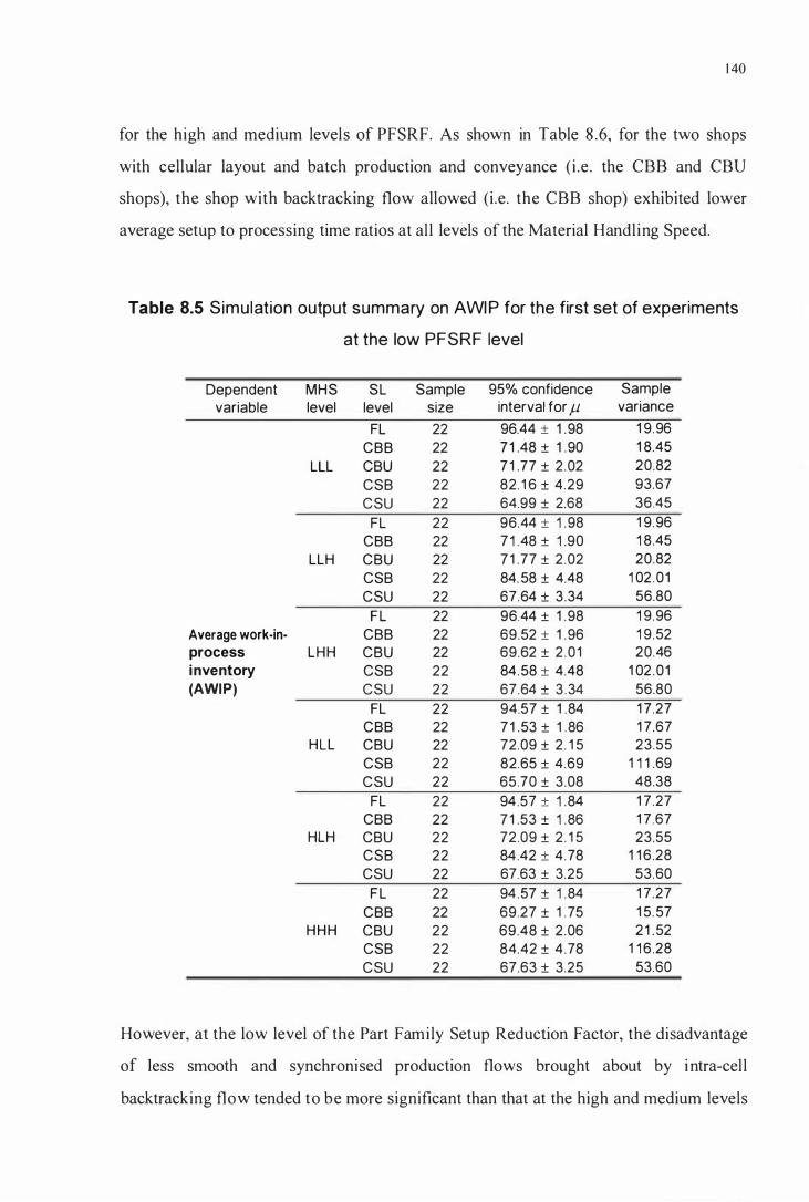
1 40

for the high and medium levels of PFSRF. As shown in Table 8 .6, for the two shops

with cellular layout and batch production and conveyance (i .e . the eBB and eBU

shops), the shop with backtracking flow allowed (i .e. the eBB shop) exhibited lower

average setup to processing time ratios at al l levels of the Material Handl ing Speed.

Table 8.5 Simulation output summary on AWI P for the first set of experiments

at the low PFSRF level

Dependent MHS SL Sample 95% confidence Sample variable level level size interval for j.1 variance

FL 22 96.44 ± 1 .98 1 9.96 eBB 22 7 1 .48 ± 1 .90 1 8.45

LLL eBU 22 7 1 .77 ± 2 .02 20.82 eSB 22 82. 1 6 ± 4.29 93.67 esu 22 64.99 ± 2.68 36.45

FL 22 96.44 ± 1 .98 1 9.96 eBB 22 7 1 .48 ± 1 .90 1 8.45

LLH eBU 22 7 1 .77 ± 2 .02 20.82 eSB 22 84. 58 ± 4.48 1 02 .01 esu 22 67.64 ± 3.34 56.80

FL 22 96.44 ± 1 .98 1 9.96 Average work·in· eBB 22 69.52 ± 1 .96 1 9.52 process LHH eBU 22 69.62 ± 2 .01 20.46 i nventory eSB 22 84.58 ± 4.48 1 02 .01 (AWIP) esu 22 67.64 ± 3 .34 56.80

FL 22 94.57 ± 1 .84 1 7.27 eBB 22 7 1 .53 ± 1 .86 1 7.67

HLL eBU 22 72.09 ± 2. 1 5 23.55 eSB 22 82.65 ± 4.69 1 1 1 .69 esu 22 65.70 ± 3.08 48.38

FL 22 94 .57 ± 1 .84 1 7 .27 eBB 22 7 1 .53 ± 1 .86 1 7 .67

HLH eBU 22 72.09 ± 2 . 1 5 23.55 eSB 22 84 .42 ± 4 .78 1 1 6 .28 esu 22 67.63 ± 3.25 53.60

FL 22 94 .57 ± 1 .84 1 7.27 eBB 22 69.27 ± 1 .75 1 5. 57

HHH eBU 22 69.48 ± 2.06 21 .52 eSB 22 84.42 ± 4 .78 1 1 6 .28 esu 22 67.63 ± 3.25 53.60

However, at the low level of the Part Family Setup Reduction Factor, the disadvantage

of less smooth and synchronised production flows brought about by intra-cel l

backtracking flow tended to be more significant than that at the high and medium levels

1 4 1

o f PFSRF. A s a result, eBB and eBU shops performed equally o n average work-in­

process inventory and average flow time because eBB shop's superior performance on

the average setup to processing time ratio was offset by the unfavourable effect of its

backtracking flow.

Table 8.6 Results of planned comparisons among cel lu lar layouts for the first

set of experiments at the low PFSRF level

Dependent MHS Ho( 1 a) Ho( 1 b) Ho(2)

variable level

LLL CBB=CBU CSU<CSB CBB+CBU=CSB+CSU

LLH CBB=CBU CSU<CSB CBB+CBU<CSB+CSU

AWI P LHH CBB=CBU CSU<CSB CBB+CBU<CSB+CSU

HLL CBB=CBU CSU<CSB CBB+CBU=CSB+CSU

HLH CBB=CBU CSU<CSB CBB+CBU<CSB+CSU

H H H CBB=CBU CSU<CSB CBB+CBU<CSB+CSU

LLL CBB=CBU CSU<CSB CBB+CBU=CSB+CSU

LLH CBB=CBU CSU<CSB CBB+CBU<CSB+CSU

AFT LHH CBB=CBU CSU<CSB CBB+CBU<CSB+CSU

HLL CBB=CBU CSU<CSB CBB+CBU=CSB+CSU

HLH CBB=CBU CSU<CSB CBB+CBU<CSB+CSU

H H H CBB=CBU CSU<CSB CBB+CBU<CSB+CSU

LLL CBB<CBU CSU<CSB CBB+CBU<CSB+CSU

LLH CBB<CBU CSU<CSB CBB+CBU<CSB+CSU

ASPTR LHH CBB<CBU CSU<CSB CBB+CBU<CSB+CSU

HLL CBB<CBU CSU<CSB CBB+CBU<CSB+CSU

HLH CBB<CBU CSU<CSB CBB+CBU<CSB+CSU

H H H CBB<CBU CSU<CSB CBB+CBU<CSB+CSU

Note: For al l sign ificant differences, p ::; 0.05.

1 42

(b) Comparison between the two cellular layout shops with single-unit production and

conveyance [by testing Ho( 1 b)]

As shown in Table 8 .6, the results of testing Ho( 1 b) show that for the cellular layout

shops with single-unit production and conveyance ( i .e . the CSU and CSB shops), the

shop with unidirectional flow (i .e . the CSU shop) always outperformed the shop with

backtracking flow ( i .e . the CSB shop). This result from testing Ho( 1 b) coincides with

the finding i l lustrated in Subsection 8 .3 . 1 that the effectiveness of unidirectional flow in

realising the advantage of single-unit production and conveyance became more

prominent at the low level of PFSRF.

(c) Comparison between the cellular layouts with BPC and the cellular layouts with

SUPC [by testing Ho(2)]

As indicated by the results of testing Ho(2) in Table 8 .6, among the shops with cellular

layout, the shops with batch production and conveyance (BPC) ( i .e . the CBB and CBU

shops) outperformed the shops with single-unit production and conveyance (the CSB

and CSU shops) on the average setup to processing time ratio for al l levels of the

Material Handling Speed. As discussed in Subsection 8 . 1 .2 , to realise the benefits of

setup time reduction through cellular manufacturing, it is essential to overcome the poor

performance in A WIP brought about by inflexible use of machines for the cellular

layout. S ince the average number of parts waiting for machine setups was smaller with a

lower average setup to processing time ratio, the effect of inflexible use of machines

was less significant for the cel lular layout shops with BPC . Therefore, the cellular

layout shops with BPC exhibited superior performance on average work-in-process

inventory and in turn, average flow time at most of the Material Handl ing Speed levels.

However, as shown in Table 8 .6, when the intra-cel l material handling speed was low

(i .e . at the LLL and HLL levels of the Material Handling Speed) the cellular layout

shops with batch production and conveyance and the cel lular layout shops with single­

unit production and conveyance had simi lar performance on A WIP and AFT. As

1 43

discussed in Subsection 8.3 . 1 , this was because the extent of decrease in AFT and

A WIP brought by unidirectional flow was relatively more significant when the intra-cel l

material handling speed was low.

(d) Comparison between the functional layout and the cellular layouts [by testing Ho(3)]

The results of the planned comparison between the cellular layouts and the functional

layout are presented in Table 8.7 . The cellular layout was found to be superior to the

functional layout on all dependent variables. This fmding coincided with that presented

in Subsection 8 .3 . 1 by examining F igure 8 .3 .

The shops with cellular layout were able to demonstrate superior performance because

the disadvantage of dedicating the machines in a cell to the processing of a family of

parts was less significant at the low level of the Part Family Setup Reduction Factor.

Therefore, the potential of cellular manufacturing in achieving lower average work-in­

process inventory and average flow time through larger extent of setup time reduction

was fully exploited.

The findings in this section show that when the extent of setup time reduction

achievable through cellular manufacturing is large (i .e . at the low level of the PFSRF),

cellular layout should be adopted for a job shop environment with Kanban-based

production control . Furthermore, the cel lular layout with SUPC and unidirectional intra­

cel l production flow should be adopted when the intra-cel l material handling speed is

low; otherwise, the cellular layout with batch production and conveyance is more

suitable.

The results and analyses of the simulation output for the first set of experiments have

been discussed in this Chapter. The factors such as the shop layout, production flow

patterns and the part family setup reduction factor were found to have substantial effects

on both the individual and relative performances of the various shops investigated. The

1 44

effect of material handling speed, however, was mainly on the relative performances

among the different shops rather than on their individual performances.

Table 8.7 Resu lts of planned comparisons between the cel lu lar and functional

layouts for the first set of experiments at the low PFSRF level

Dependent MHS Ho(3)

variable level

LLL (CBB+CBU+CSB+CSU)/4<FL

LLH (CBB+CBU)/2<FL

AWI P LHH (CBB+CBU)/2<FL

HLL (CBB+CBU+CSB+CSU)/4<FL

HLH (CBB+CBU)/2<FL

HHH (CBB+CBU)/2<FL

LLL (CBB+CBU+CSB+CSU)/4<FL

LLH (CBB+CBU)/2<FL

AFT LHH (CBB+CBU)/2<FL

HLL (CBB+CBU+CSB+CSU)/4<FL

HLH (CBB+CBU)/2<FL

H H H (CBB+CBU)/2<FL

LLL (CBB+CBU)/2<FL

LLH (CBB+CBU)/2<FL

ASPTR LHH (CBB+CBU)/2<FL

HLL (CBB+CBU)/2<FL

HLH (CBB+CBU)/2<FL

HHH (CBB+CBU)/2<FL

Note: For a l l significant d ifferences, p � 0.05.

Following the first set of experiments, a second set of experiments was performed to

investigate the influence of the variabil ity of processing and setup times on the

1 45

performance of a Kanban-control led job shop. The design of the second set of

experiments will be i l lustrated in Chapter 9. The results and analyses of the simulation

output for the second set of experiments will be discussed in Chapter 1 0 .

1 46

CHAPTER 9

DESIGN AND EXECUTION OF THE SECOND SET OF EXPERIMENTS - FOR

INvESTIGATING THE EFFECTS OF THE VARIABILITY OF SETUP AND

PROCESSING TIMES

The effects of four influential factors : shop layout, production flow patterns, material

handling speed and the part family setup reduction factor on the performance of a

Kanban-control led job shop have been investigated in the first set of experiments. The

variabi lity (or coefficients of variation) of setup and processing times was fixed

throughout the experiments. By investigating the results from the first set of

experiments we found that the synchronisation (balance) of operations had a significant

effect on the performance of the cel lular layout shop with single-unit production and

conveyance (See Subsection 8 . 1 . 1 ) . In addition, the influence of the variabil i ty of

processing time on a Kanban-based system had been emphasised by both Philipoom et

al. ( 1 987) and Villeda et al. ( 1 988).

Because operations tend to be less synchronised when setup and processing times are

more variable, the effect of changing the coefficients of variation (CVs) of setup and

processing times on the performance of a Kanban-control led job shop may be important.

To gain more understanding of this subject, the second set of experiments was thus

carried out to examine the behaviour of the shop at different levels of the CV s for setup

and processing times.

This chapter covers six parts, namely :

( 1 ) design of the experimental system,

(2) selection of the independent variables and their levels to be investigated,

(3) selection of the dependent variables to be measured,

(4) settings of material handling speed,

(5) selection of the appropriate statistical analyses of the simulation output, and

(6) development and operation of the simulation model.

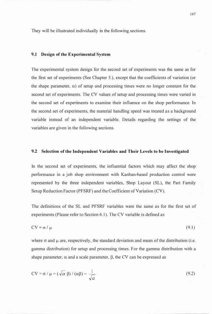
They will be i l lustrated individually in the following sections.

9. 1 Design of the Experimental System

1 47

The experimental system design for the second set of experiments was the same as for

the ftrst set of experiments (See Chapter 5 . ) , except that the coefficients of variation (or

the shape parameter, a) of setup and processing times were no longer constant for the

second set of experiments. The CV values of setup and processing times were varied in

the second set of experiments to examine their influence on the shop performance. In

the second set of experiments, the material handling speed was treated as a background

variable instead of an independent variable. Details regarding the settings of the

variables are given in the fol lowing sections.

9.2 Selection of the Independent Variables and Their Levels to be I nvestigated

In the second set of experiments, the influential factors which may affect the shop

performance in a j ob shop environment with Kanban-based production control were

represented by the three independent variables, Shop Layout (SL), the Part Family

Setup Reduction Factor (PFSRF) and the Coefficient of Variation (CV).

The deftnitions of the SL and PFSRF variables were the same as for the ftrst set of

experiments (Please refer to Section 6. 1 ) . The CV variable is deftned as

CV = er / I-! (9. 1 )

where er and � are, respectively, the standard deviation and mean of the distribution (i .e .

gamma distribution) for setup and processing times. For the gamma distribution with a

shape parameter, a and a scale parameter, �, the CV can be expressed as

CV = er / � = ( ra �) / (a�) = _I_ ra

(9.2)

1 48

Thus the coefficient of variation for the gamma distribution can be set by simply

changing the a value. In this set of experiments, both setup and processing time CVs

had high, medium and low settings. The values of the three CV settings for setup and

processing times are summarised in Table 9. 1 .

Table 9.1 Values for the setup and processing time CV settings

CV Setting CV value for

Setup time Processing time

High 1 .06 (a = 0.89) 0.87 (a = 1 . 33) _._.-

Med ium 0.71 (a = 2 .00) 0 .58 (a = 3 .00)

Low 0.47 (a = 4 .50) 0 .38 (a = 6.75)

Note: a IS the shape factor of the gamma distribution for the corresponding CV value.

The levels investigated for the three independent variables are summarised in Table 9.2.

The levels for the Shop Layout and Part Family Setup Reduction Factor were the same

as for the first set of experiments.

For the Coefficient of Variation, each of the three (high, medium and low) setup time

CV settings was investigated with each of the three processing time CV settings.

However, in a wel l managed job shop, the level of processing time variabi lity is not

l ikely to be higher than that of the setup time variabil ity (Mahrnoodi et al. 1 990).

Therefore, the CV levels at which processing time CV settings are higher than setup

time CV settings (i .e . the MH, LH and LM levels of CV) were not investigated. I n total,

six levels of the Coefficient of Variation variable were investigated. Thus, the second

set of experiments was· based on the 5 x 3 x 6 ful l factorial design, with five, three and

six levels for the SL, PFSRF and CV independent variables, respectively.

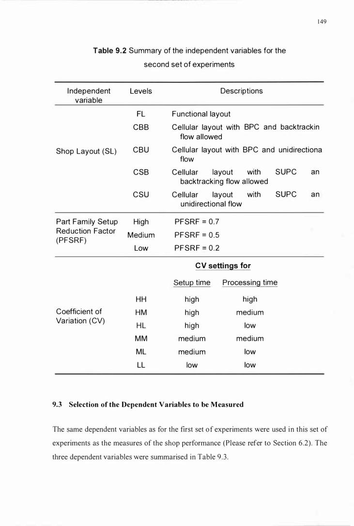
Table 9 .2 Summary of the independent variables for the

second set of experiments

I ndependent Levels Descriptions variable

FL Functional layout

1 49

CBB Cel lu lar layout with BPC and backtrackin flow al lowed

Shop Layout (SL) CBU Cel lu lar layout with BPC and unid irectiona

CSB

CSU

Part Fami ly Setup High Red uction Factor Med ium (PFSRF)

Low

HH

Coefficient of HM Variation (CV)

HL

MM

ML

LL

flow

Cel lular layout with SUPC backtracking flow a l lowed

Cel lular layout with SUPC un id i rectional flow

PFSRF = 0.7

PFSRF = 0 .5

PFSRF = 0 .2

CV settings for

Setup time Processing time

h igh h igh

h igh medium

h igh low

med ium medium

med ium low

low low

9.3 Selection of the Dependent Variables to be M easured

an

an

The same dependent variables as for the first set of experiments were used in this set of

experiments as the measures of the shop performance (Please refer to Section 6.2) . The

three dependent variables were summarised in Table 9 .3 .

1 50

Table 9.3 Summary of the dependent variables for the

second set of experiments

Dependent variable

Average work- in­process inventory (AWI P)

Average flow time (AFT)

Average setup to processing time ratio (ASPTR)

Descriptions

Total number of parts in the system, averaged over the observation time period .

The amount of time spent by a part from entering the system unti l the completion of al l operations, averaged over a l l completed parts during the observation t ime period .

Ratio of total amount of time spent for setting up machines to total amount of time spent for processing parts, averaged over a l l mach ines in the observation time period .

9.4 Settings of the M aterial Handling Speed

In the second set of experiments, the material handl ing speed was treated as a

background variable, which potentially could affect the dependent variables in the

experiments but was not of interest as a independent variable. S ince the dependent

variables were affected by the background variables as wel l as the independent variables,

the setting of the background variable was control led in the experiments so that the

effect of the independent variables was not distorted.

Therefore, in the second set of experiments, all material handling speeds except those

for backtracking flow were set at their high settings, unless the results of the planned

comparisons in the first set of experiments showed that low material handl ing speed

settings led to better performance for some layouts. In this way, we could be sure that

more efficient material handl ing facilities were used for all shops so that the

performances of different shops could be compared on a equal basis, and the bias caused

by different material handl ing speed settings was minimised.

1 5 1

For example, from Table 8 .2, we knew that at the high PFSRF level, the CBU shop

exhibited better performance on average flow time and average setup to processing time

ratio when both inter-cel l and intra-cell material handling speeds were at low settings.

Therefore, the low settings of both inter-cel l and intra-cell material handling speeds

were used for the CBU shop when running the simulation. The settings of the material

handling speeds for the various levels of the Shop Layout and Part Family Setup

Reduction Factor independent variables are summarised in Table 9.4.

Table 9.4 Settings of Material hand l ing speeds for the

second set of experiments

PFSRF level SL level

FL eBB eBU eSB esu

0.7 high, - high, high low, low high, h igh high, h igh

0 .5 high, - high, low low, high high , high high, high

0.2 high, - high, high high, high high, low high, low

Note: For each entry, the first setting IS for Inter-cel l (department) material handling and the second, for intra-cel l material handling .

The same design of the high and low settings for the material handl ing speed as for the

first set of experiments was used in this set of experiments. Tables 9.5 gives the material

handling speed settings for inter-cel l / department part movement. Tables 9.6 and 9.7

show the material handling speed settings for intra-cel l part movement with batch

production and conveyance, and single-unit production and conveyance, respectively .

9.5 Selection of the Appropriate Statistical Analyses of the Simulation Output

Similar to the experimental design for the first set of experiments, the overall F-test and

planned comparison were employed for analysing the results of the experiments.

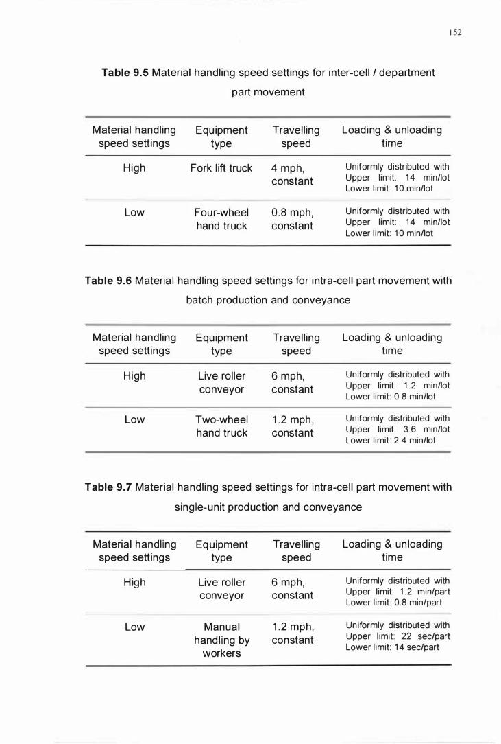
1 52

Table 9.5 Material handl ing speed settings for inter-cel l / department

part movement

Material handl ing speed settings

High

Low

Equ ipment type

Fork l ift truck

Four-wheel hand truck

Travel l ing speed

4 mph, constant

0 .8 mph, constant

Load ing & unload ing time

Uniformly distributed with Upper l imit: 1 4 min/lot Lower l imit: 1 0 min/lot

Uniformly d istributed with Upper l imit: 1 4 min/lot Lower l imit: 1 0 min/lot

Table 9.6 Materia l handl ing speed settings for intra-cel l part movement with

batch production and conveyance

Material handl ing speed sett ings

High

Low

Equ ipment type

Live rol ler conveyor

Two-wheel hand truck

Travel l ing speed

6 mph, constant

1 .2 mph , constant

Load ing & unload ing time

Uniformly distributed with Upper l imit: 1 .2 min/lot Lower l imit: 0 .8 minllot

Un iformly d istributed with Upper l imit: 3 .6 min/lot Lower l imit: 2.4 min/lot

Table 9 .7 Material handl ing speed settings for intra-cel l part movement with

sing le-un it production and conveyance

Materia l handl ing Eq u ipment Travel l ing Load ing & un load ing speed settings type speed time

H igh Live rol ler 6 mph, Uniformly d istributed with

conveyor constant Upper l imit: 1 .2 min/part Lower l imit: 0.8 min/part

Low Manual 1 . 2 mph, Uniformly distributed with

hand l i ng by constant Upper l imit: 22 sec/part

workers Lower l imit: 1 4 sec/part

9.5 . 1 Statistical output analyses by the F-test

1 53

The overall F-test was used to detect whether there was any differences in the shop

performances attributed to the different levels of the Shop Layout variable. A One-way

analysis of variance (ANOV A) was carried out for each of the three dependent variables

at each of level of the PFSRF and CV variables. Therefore in total 3x3x6 = 54

ANOV As were performed to achieve the results of the overall F-tests.

9 .5 .2 Statistical output analyses by the planned comparison

As i l lustrated in Subsection 6.3 .2, because overall F-tests by ANOV As did not tell

where the differences came from if there was any, Lindman's planned comparison was

used to pinpoint the causes of differences by answering the research questions put

forward in Chapter 4 . Research questions 1 and 2 were the same as those addressed by

the first set of experiments (See Subsection 6.3 .2). They are as fol lows:

Research question 1 : Do shop layout and part flow patterns have any influence on the

performance of a Kanban-control led job shop? This question is addressed through the

fol lowing four sub-questions.

Sub-question 1 . 1 : For the cel lular layout shops with batch production and

conveyance (BPC), is there any difference in performance between the shop with

backtracking flow allowed and the shop with unidirectional flow ?

Sub-question 1 .2 : Simi lar to Sub-question 1 . 1 , but for the cellular layout shops with

single-unit production and conveyance (SUpe).

Sub-question 1 .3 : Among the shops with cellular layouts, are those with BPC

different from those with SUPC in their performance ?

Sub-question 1 .4 : I s there any difference between functional layout and cellular

layout in terms of shop performance ?

1 54

Research question 2 : How does the extent of setup time reduction through cellular

manufacturing affect the performances of the shops with the various layouts and flow

patterns ?

Research question 3 had been addressed by the first set of experiments. For the second

set of experiments, we addressed another research question, namely,

Research question 4 : To what extent do the coefficients of variation (CVs) of machine

setup times and part processing times influence the performances of the shops with the

various layouts and flow patterns ?

To answer Research question 1 (or Sub-questions l . 1 through 1 .4), the same hypotheses

expressed by equations (6. 1 ) through (6.6) in Subsection 6 .3 .2 were tested for each

dependent variable at each level of the Coefficient of Variation and Part Fami ly Setup

Reduction Factor independent variables. Research questions 2 and 4 were answered by

comparing the results of planned comparisons across the different levels of the PFSRF

and CV variables, respectively. The same formulas for the Approximate F-test as

i l lustrated in Subsection 6 .3 .2 were used for testing the proposed hypotheses.

9.6 Development and Operation of the Simulation M odel

The same simulation model coded in the SIMSRIPT 1 1 . 5 simulation language as

i l lustrated in Section 7 .2 was used for the second set of experiments.

In order to observe whether the initial transient period used for the first set of

experiments was sufficient for the higher CV values used in this set of experiments,

prel iminary simulation runs were performed for the CSB shop with the high level of

PFSRF and HH level of CV (i .e . the worst case). The Welch's graphical procedure, as

depicted in Subsection 7.4. 1 was fol lowed to study the initial transient periods. The

moving average plot for average work-in-process inventory presented in Figure 9. 1

shows that the initial transient period of 48 periods (5760 hours) used for the first set of

1 55

experiments was sufficient for this set of experiments. The moving average plots for all

the dependent variables are given in Appendix 1 1 .

200 '" t '" c.!:" 1 50 o ...

� 1 00 E ::s

Z 50

o

Period ( 1 20 hrs )

Figure 9 .1 Moving average plot for average work-in-process i nventory

(Cel lu lar layout with SUPC and backtracking flow al lowed)

As described in Subsection 7 .4 .3 , the revised blocking method was employed to obtain

independent observations of the statistics on the dependent variables, and the method of

batch means was util ised to obtain the estimations of sample variances, sample means

and the confidence intervals of population means for the dependent variables. The same

numbers of Kanbans and containers as determined in Subsection 7.4.2 were used for the

second set of experiments.

CHAPTER 1 0

ANALYSES AND DISCUSSIONS OF THE SIMULATION RESULTS FOR

THE SECOND SET OF EXPERIMENTS

1 56

The results and discussions of the simulation output and statistical output analyses for

the second set of experiments are presented in this chapter. As explained at the

beginning of Chapter 8, to compare the different shops on the same basis, the results

were presented and discussed for each of the high, medium and low levels of the Part

Family Setup Reduction Factor separately. The influence of the Part Family Setup

Reduction Factor itself was examined by comparing the results across the three PFSRF

levels.

10.1 Simulation Results and Discussions for the H igh PFSRF Level

As presented in Chapter 8, the simulation output was analysed in two ways for each of

the part family setup reduction factor levels. F irst, the graphical method was used. The

differences in the performances of individual shops were examined by presenting the

simulation output in bar charts. Next, the hypotheses proposed in Section 9.5 were

tested, and results and discussions were presented. By using the two analysis methods,

the maximum amount of information could be extracted from the simulation output.

1 0 . 1 . 1 Discussions of the simulation output presented in bar charts

The sample mean values on the three dependent variables, average work-in-process

inventory (A WIP), average flow time (AFT) and the average setup to processing time

ratio (ASPTR) from the second set of experiments at the high PFSRF level are

presented in Figure 1 0 . 1 .

1 57

As shown in Figure 1 0 . 1 , the performances of the cel lular layout shops with single-unit

production and conveyance (SUPC) ( i .e. the CSB and CSU shops) were greatly inferior

to those of other shops.

The influence of the Coefficient of Variation (CV) for processing times was dominant

for the cellular layout shops with single-unit production and conveyance. When the CV

level changed from HH to BM (Note the second letter indicates the processing time CV

setting), the performances of the CSB and CSU shops on all dependent variables were

greatly improved. These changes were significant since there was no overlap between

the 95% confidence intervals. However, the influence of the processing time CV was

lessened when the setup time CV setting was medium or low ( i .e. at the MM, ML and

LL levels of CV). The average work-in-process inventory and average flow time for the

cellular layout shop with SUPC and unidirectional flow (i .e . the CSU shop) were further

improved as the Coefficient of Variation reached the LL level .

The effect of the CV of setup times on the performances of the cellular layout shops

with single-unit production and conveyance was not as important as that of processing

times. For example, by comparing the bar graphs at the HL and ML levels of CV for the

CSU shop, we found that the performances seemed to be improved at the ML level .

However, we are not confident about these differences since there were overlaps

between the corresponding 95% confidence intervals.

As explained in Subsection 8 . 1 . 1 , the inferior performance of the cellular layout shops

with single-unit production and conveyance at the high PFSRF level was mainly due to

prominent effect of less synchronised operations caused by SUPe. Since operations

tended to be more synchronised with a lower processing time CV, decreasing the

processing t ime CV was therefore more effective in improving the performance of the

cellular layout shops with single-unit production and conveyance. However, reducing

the coefficient of variation of processing times was not sufficient to make the

performances of the CSB and CSU shops superior to those of other shops ( i .e. the FL,

CBB and CBU shops) .

300

r:::::- 250 -1 * 0

1 1 200 u. a::: CJ) 1 50 u. � a.. �

50 «

0 HH HM HL MM ML

Le\el of CV

* The error l ines indicate the 95% confidence intervals for J.1 .

45

40 -

r:::::- 35 0 T 1 1 30 -

u. a::: 25 CJ) u. 20 a.. f- 1 5 u. 1 0 «

5

0

HH

I 4.5

4.0 r:::::-

3.5 0 1 1

3.0 u.

- r 11 - -

- -a::: (f) 2.5 u. r - F a.. 2.0 - -� -

a::: 1 .5 f-a.. 1 .0 (f) « 0.5

0 .0 HH

HM

-tor=\

I -� f

..

�. HM

HL MM

Le\el of CV

-� �l

F . '-'" l =

�

I HL MM

Le\el of CV

ML

.t1

I t �

�

r ML

LL

T

LL

'9 � --

1-1- -

1- I"" l-f-r--

LL

- -- -----,

rm F L

. CBB O CBU

I · CSB o CSU

--l � - I • FL

. CBB I O CBU I . CSB J � 0 CSU I

-I -

r;FLl I · CBB o CBU I . CSB I

l o CSU l 1

1 58

Figure 1 0. 1 Simu lation output summary of the second set of experiments at

PFSRF level = High

1 59

I t is interesting to note that when the Coefficient of Variation reached the LL level, the

performance of the CSB shop tended to be worse. This finding indicates the importance

of unidirectional flow for realising the advantage of reducing setup and/or processing

time variabil ity (or coefficient of variation).

In other words, the advantage of reducing setup and/or processing variabil ity can only

be realised when parts flow smoothly throughout the cel l . In a cellular layout with

backtracking flow allowed, although parts flow through a workstation smoothly with

low variabil ity in setup and processing times, congestion of part flow in the cell may

stil l happen when they backtrack to another workstation. Eventually, the advantage

brought about by the reduction in setup and/or processing time variabil ity was offset by

the adverse effect of backtracking flow. As we found in Figure 1 0. 1 , the effect of

backtracking flow may even be amplified by reducing the CV of setup and/or

processing times without reducing the setup times themselves (or the part family setup

reduction factor).

Furthermore, for the two cellular layout shops with single-unit production and

conveyance, the shop with unidirectional flow (i .e. the CSU shop) tended to outperform

the shop with backtracking flow allowed (i .e . the CSB shop). Particularly, at the LL

level of the Coefficient of Variation variable, the difference was significant since there

was no overlap between their 95% confidence intervals for the dependent variables.

Hence, we may conclude that at the high Part Family Setup Reduction Factor level, the

more synchronised operations brought about by unidirectional flow was most effective

in improving the performance of the cel lular layout with single-unit production and

conveyance when both setup and processing time CV settings were low. However, with

the high PFSRF level, unidirectional intra-cel l flow was not sufficient to make the

performances of the cellular layout shops with single-unit production and conveyance

superior to other shops.

The influence of the Coefficient of Variation on the performances of the remaining

shops ( i .e . FL, CBB and CBU shops) was dominated by the CV setting of the setup

1 60

times. When the setup time CV changed from the high to medium setting ( i .e. from HM

to MM of the CV level), their performances on A WIP and AFT were significantly

improved (i .e. no overlap among the individual 95% confidence intervals). Since setup

times were longer at the high level of the Part Family Setup Reduction Factor, the

performances of those shops were dominated by setup times. I t was therefore reasonable

that the effect of the setup time CV on their performances was more important.

1 0. 1 .2 Discussions of the results of overall F-tests and planned comparisons

As mentioned in Subsection 8 . 1 .2, the bar charts given in Figure 1 0 . 1 were most useful

for examining the differences in the performances of individual shops over the different

Coefficient of Variation levels. However, the use of bar charts i n comparing the

performances of different shops, particularly for the comparison between groups of

shops (e.g. comparing the functional layout shop with all the cel lular layout shops), was

l imited.

Overall F-tests and planned comparisons were more powerful for comparmg the

performances between different shops than the bar charts. The differences in the

performances among different shops could be identified more preci sely with specific

levels of significance. In addition, planned comparisons were particularly useful for

comparing groups of shops.

Table 1 0 . 1 shows the sample means, sample variances and 95% confidence intervals of

population means for the average work-in-process inventory at the high level of the Part

Family Setup Reduction Factor. We can see that the performances of the cellular layout

shops with single-unit production and conveyance (i .e. the CSB and CSU shops) were

extremely variable (The output summary of the all three dependent variables are given

in Tables A I 2 . 1 -3 of Appendix 1 2). As explained in Subsection 8 . 1 .2, to avoid the

overall F-tests being biased by the large variances, and to increase the power of the

Approximate F test for the planned comparisons, the data for the CSB and CSU were

not included in the overall F-tests and planned comparisons.

1 6 1

Table 1 0. 1 Simu lation output summary o n AWI P for the second set of

experiments at the h igh PFSRF level

Dependent CV SL Sample 95% confidence Sample variable level level size interval for f.1 variance

FL 22 60.08 ± 1 . 37 9.60 eBB 22 65.06 ± 2. 1 3 23. 1 7

H H eBU 22 70.03 ± 2.85 4 1 .41 CSB 22 2 1 9 .88 ± 25.08 3 1 99.0 CSU 22 1 99.27 ± 2 1 .63 2380.3 1

FL 22 59.63 ± 1 .45 eBB 22 64.92 ± 1 .96 1 9.45

HM eBU 22 70. 33 ± 2 .74 38.25 CSB 22 1 59.37 ± 1 3.94 989.08 CSU 22 1 47 .66 ± 1 2.91 847 .39

22 59.43 ± 1 . 56 1 2.36 Average work·in· 22 65.66 ± 2 .64 35.5 1 process H L 22 68.86 ± 2. 1 7 24.05 inventory 22 1 53. 1 1 ± 1 3.60 �O.&l (AWIP) 22 1 4 1 .37 ± 16.08 1 31 5.5 1

22 58 . 1 1 ± 1 . 36 9.39 eBB 22 60.63 ± 1 .96 1 9.49

MM eBU 22 63.92 ± 1 .99 20.20 CSB 22 1 45.09 ± 1 2.79 832.44 CSU 22 1 29.72 ± 1 1 .9 1 721 .6 1

FL 22 58.09 ± 1 .35 9.22 eBB 22 60.56 ± 1 . 9 1 1 8.46

ML eBU 22 63.08 ± 1 .76 1 5.82 CSB 22 1 4 1 .62 ± 1 4 .89 1 1 27.75 CSU 22 1 2 1 .53 ± 1 1 .83 71 2.20

FL 22 57.22 ± 1 .29 8.45 eBB 22 58.28 ± 1 .64 1 3.67

LL eBU 22 6 1 . 53 ± 1 .72 1 5.08 eSB 22 1 53 .59 ± 1 9.04 1 843.50 CSU 22 1 1 3 .32 ± 1 0.47 557.69

Since the data for the CSB and CSU shops were not included In the planned

comparisons, the two null hypotheses:

Ho( 1 b): Iless = Ilesu and

Ho(2) : lleSB + lleBU = lleSB + Ilesu

were not tested. Ho(3) was then reduced to

Ho(3) : IlFL = 1 I2CIlcss + IlCBU)

1 62

The overall differences among the Shop Layout (SL) levels were found to be significant

through the overall F-tests at all levels of the Coefficient of Variation variable, with

significance levels lower than 0.00 1 (See Table A 1 3 . 1 of Appendix 1 3 for details). The

results of the hypothesis tests are discussed individually as fol lows.

(a) Comparison between the two cel lular layout shops with batch production and

conveyance [by testing Ho( l a)]

The results of the planned comparisons for the high Part Family Setup Reduction Factor

level are presented in Table 1 0.2 (See Table A I 4. 1 -3 of Appendix 1 4 for detai ls).

As indicated by the results of testing Ho( 1 a), for the cellular layout shops with batch

production and conveyance (BPC), the shop with backtracking flow allowed (i .e . the

CBB shop) outperformed the shop with unidirectional flow (i .e . the CBU shop) on

A WIP and AFT at all but the HL levels of CV. Some differences in average setup to

processing time ratio between the CBB and CBU shops were also identified (at HH, HL

and MM levels of the Coefficient of Variation). However, no specific pattern could be

found to explain these differences. These differences in the performances between the

two shops were l ikely to be attributed to the different material handling speed settings.

The above finding shows that as long as more efficient material handl ing faci lities were

employed, backtracking intra-cell flow was more advantageous for improving the

performance (on A WIP and AFT) of the cellular layout with batch production and

conveyance, at the high PFSRF level .

Recal l that the cellular layout with backtracking flow allowed had been designed by

keeping inter-cel l part movement to a minimum (See Subsection 5 .2 . 1 for details).

When parts were transported (in batches) among cel ls more often (as for the cellular

layout with unidirectional flow), parts had more chances to be queued in front of a

workstation with other parts not only from other workstations in the cel l , but also from

other cel ls . On the other hand, for the cellular layout with backtracking flow allowed,

1 63

most parts visited only one cell and therefore, the congestion of parts was lessened.

Particularly, the advantage of backtracking flow was prominent with the high level of

the Part Family Setup Reduction Factor since parts spent more time in waiting for

machine setups. Consequently, backtracking flow was effective in reducing the waiting

times, and leading to the superior performance of the CBB shop.

Table 1 0.2 Resu lts of planned comparisons for the second set of experiments

at the high PFSRF level

Dependent CV Ho( 1 a) Ho(3)

variable level

H H CBB<CBU FL « CBB+CBU)/2

H M CBB<CBU FL « CBB+CBU)/2

AWI P HL CBB=CBU FL « CBB+CBU)/2

M M CBB<CBU FL « CBB+CBU)/2

ML CBB<CBU FL « CBB+CBU)/2

LL CBB<CBU FL « CBB+CBU)/2

HH CBB<CBU FL « CBB+CBU)/2

HM CBB<CBU FL « CBB+CBU)/2

AFT HL CBB<CBU FL « CBB+CBU)/2

M M CBB<CBU FL « CBB+CBU)/2

ML CBB<CBU FL « CBB+CBU)/2

LL CBB<CBU FL « CBB+CBU)/2

HH CBB<CBU FL>(CBB+CBU)/2

H M CBB=CBU FL>(CBB+CBU)/2

ASPTR HL CBB<CBU FL>(CBB+CBU)/2

MM CBB<CBU FL>(CBB+CBU)/2

M L CBB=CBU FL>(CBB+CBU)/2

LL CBB=CBU FL>(CBB+CBU)/2

Note: For al l sign ificant differences, P ::; 0 .05.

1 64

(b) Comparison between the functional layout and the cellular layouts [by testing Ho(3 )]

The comparison between the functional layout (i .e . FL) and the cellular layouts ( i .e.

CBB and CBU) through Ho(3 ) shows that the average setup to processing time ratios of

the cellular layout shops were lower than those of the functional layout for all levels of

the Coefficient of Variation variable. This outcome demonstrated that the higher

potential of cellular manufacturing in capitalising on the similarities of operation

sequences among different part types to achieve setup time reduction was not affected

by the setup and processing time CV values. However, despite the superior performance

of the cellular layout shops on ASPTR, the functional layout shop outperformed the

cellular layout shops on A WIP and AFT for all CV levels.

As i l lustrated in Subsection 8 . 1 .2, in a cellular layout, a machine was only permitted to

process the fami ly of parts assigned to it. Because of the inflexibility in the use of

machines, machines tended to be less utilised and build-up of queues was more l ikely to

happen . On the other hand, in the functional layout, when a job arrived at a department

with interchangeable machines of the same type, it could be processed on any machine

that was avai lable. Consequently, inflexible use of machines rendered the performances

of the cellular layout shops on the average work-in-process inventory and the average

flow time inferior to those of the functional layout shop.

The findings in both this section and Section 8 . 1 show that functional layout should be

more suitable for a job shop environment with Kanbans when the extent of setup time

reduction achievable through cellular manufacturing is smal l ( i .e . at the high level of the

Part Family Setup Reduction Factor). The superior performance of the functional layout

was found to be robust with respect to the levels of both material handling speed, and

setup and processing time CV s.

Note that the (statistical ly) significant differences identified through the planned

comparisons seem not so important (in practice) on the bar charts given in Figure 1 0. 1 .

As explained in Subsection 8. 1 .2, the statistically significant differences do provide

important guidelines for industrial applications. In addition, differences that may not

1 65

appear to be practically important in a simulated shop environment may turn out to be

important in a real shop environment.

The results and analyses of the simulation output for the medium level of the Part

Family Setup Reduction Factor will be discussed in the next section.

10.2 Simulation Results and Discussions for the Medium PFSRF Level

As for the high PFSRF level, the discussions in this section is also divided into two

parts. First, bar charts for the sample means and 95% confidence intervals of the three

dependent variables are used to examine the differences in the shop performances

caused by the different levels of the Coefficient of Variation variable. Then, the results

from the overall F-test tests and planned comparisons are presented and discussed.

1 0 .2 . 1 Discussions of the simulation output presented in bar charts

Figure 1 0 .2 shows the sample means and the 95% confidence intervals of population

means for the dependent variables at the medium level of the Part Family Setup

Reduction Factor.

As found for the high PFSRF level, the influence of changing the Coefficient of

Variation level was most important for the cellular layout shops with single-unit

production and conveyance (i .e . the CSB and CSU shops). The effect of the changes in

the CV level on the performances of the CSB and CSU shops was sti l l dominated by the

processmg time CV setting (Note the second letter in the CV level represents the

processmg time CV setting) . The effect of the Coefficient of Variation was most

substantial as the processing time CV setting changed from high to medium when the

setup time CV setting was high (i .e . when the CV level changed from H!"J to HM).

Furthermore, reducing the variability (or coefficients of variation) of setup and

processing times was more effective in improving the performance of the CSU shop.

1 80

1 60

LO ci

1 40 f-1 1 1 20

ll.. c::: 1 00 Cl)

-

ll.. 80 , Q:.. I-

a... 60 i= -,'" � 40 -

« 20 -

0 HH

25

LO 20 f-ci 1 1

1 5 ll.. -

c::: Cl) ll..

1 0 Q:.. -

l-.... ,�

ll.. 5 «

0 HH

3.0

LO 2.5 -

ci 1 1 2.0 ll.. �

c::: Cl) ll.. 1 .5 Q:.. �� c::: 1 .0 I- -

a... Cl) 0.5 «

0.0 HH

h I L -

'" ,�

f I

HM

-� r -

.... -�

,

I± ""

I-

-

HM

- -

l--

HM

:q - ff' tl - r - ,

_1" = r'--r"" r , [

, .

HL M\1

Le-.el of CV

-

-� � j� - -

Lr .... � .... I

, .

HL M\1

Le-.el of CV

1 ;r et, r'" ..- -

f [ � I , 1-- l-.... .

l I--l- f I . HL M\1

Le-.el of CV

I--- If--�--z

r ML LL

-

- � � F

ML LL

F-T -

"' 0-

f- � I""

I l ML LL

-

--

-

I-iL -I

� -

- -�i-�

rr >--

� � � I

- -

1 111 FL I . CBB \ o CBU . CSB I _�CS�

r;T=L • CBB , O CBU I 1 . CSB c CSU l 1

l1li FL I · CBB o CBU . CSB o CSU

L _--1

Figure 1 0.2 Simu lation output summary of the second set of experiments

at PFSRF level = Med ium

1 66

1 67

As shown in F igure 1 0.2, when the CV level decreased from HM to LL, the A WIP and

AFT performances of the CSU shop were continuously improved while there was no

significant change in the performance of the CSB shop. As explained in Subsection

1 0 . 1 . 1 , the advantage of reducing setup and processing time variabil ity can only be

realised when parts flow smoothly throughout cells for the cellular layout with single­

unit production and conveyance. Therefore, unidirectional flow was essential for \

realising the benefit of reducing setup and processing time variability for the cellular

layout with single-unit production and conveyance because production flow tended to

be smoother with unidirectional flow.

The same as for the high PFSRF level, the performances of the cellular layout shops

with single-unit production and conveyance ( i .e. the CSB and CSU shops) were still

inferior to those of other shops (i .e. the FL, CBB and CBU shops) on all the three

dependent variables. The medium level of the Part Family Setup Reduction Factor was

stil l not sufficient to entirely overcome the disadvantage of less synchronised operations

caused by single-unit production and conveyance (Refer to Subsection 8 . 1 . 1 ) .

However, some drastic changes in the performances of the cellular layout shops with

single-unit production and conveyance were identified at this medium level of Part

Family Setup Reduction Factor. As shown in Figure 1 0 .2, between the cel lular layout

shops with single-unit production and conveyance, the shop with unidirectional flow (i .e.

the CSU shop) outperformed the shop with backtracking flow allowed (i .e. the CSB

shop) over all CV levels for all three dependent variables. The differences in the

performances of the two shops were significant because there was no overlap between

their 95% confidence intervals.

This finding about the effectiveness of unidirectional flow in improving the

performance of the cellular layout with single-unit production and conveyance coincide

with the outcome found in Subsection 8 .2 . 1 . When parts flowed in the same forward

direction ( i .e . with unidirectional flow) in a cell, production flows tended to be smoother

and more synchronised than with backtracking flow allowed. Consequently,

1 68

unidirectional flow was effective in alleviating the disadvantage of less synchronised

operations brought about by single-unit production and conveyance (Please refer to

Subsection 8 . 1 . 1 ) . Since both the first and second sets of experiments resulted in the

same finding, we are confident that the effectiveness of unidirectional flow in improving

the performance of the cellular layout shop with single-unit production and conveyance

was robust with respect to material handling speed and variabil ity ( i .e . the coefficient of

variation) of setup and processing times.

For the cellular layout shops with batch production and conveyance (i .e . the eBB and

CBU shops) and the functional layout (FL) shop, their performances were still

dominated by the setting of the setup time coefficient of variation. The average work-in­

process inventory and average flow time of the eBB and CBU shops were significantly

improved (i .e . no overlap for the 95% confidence intervals) as the setup time CV setting

decreased from high to medium (i .e . The CV level changed from HM to MM). However,

for the functional layout shop, only the average flow time was improved when the

setting of the setup time coefficient of variation changed from high to medium.

As depicted in Subsection 1 0 . 1 . 1 , the effect of the setup time CV setting on the

performances of the cellular layout shops with batch production and conveyance was

more significant because the performances of these shops were sti l l dominated by setup

times at the medium PFSRF level .

1 0 .2.2 Discussions of the results of overall F-tests and planned comparisons

Overall F-tests and planned comparisons were carried out to identify the differences in

the shop performances caused by the different levels of the Shop Layout variable. In

comparison with bar charts, Overal l F-tests and planned comparisons were more

powerful for comparing the performances between different shops. I n addition, planned

comparisons were particularly useful for comparing groups of shops.

Table 1 0 .3 shows the sample means, sample variances and 95% confidence intervals of

population means for the average work-in-process inventory at the medium level of the

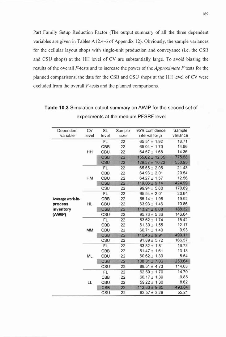
1 69

Part Family Setup Reduction Factor (The output summary of al l the three dependent

variables are given in Tables A 1 2 .4-6 of Appendix 1 2) . Obviously, the sample variances

for the cellular layout shops with single-unit production and conveyance (i .e . the CSB

and CSU shops) at the HH level of CV are substantially large. To avoid biasing the

results of the overall F-tests and to increase the power of the Approximate F tests for the

planned comparisons, the data for the CSB and CSU shops at the H H level of CV were

excluded from the overall F-tests and the planned comparisons.

Table 1 0.3 Simu lation output summary on AWI P for the second set of

experiments at the med ium PFSRF level

Dependent CV SL Sample 95% confidence Sample variable level level size interval for f-L variance

FL 22 65.51 ± 1 .92 1 8.7 1 eBB 22 65.04 ± 1 .70 1 4.66

HH eBU 22 64.57 ± 1 .68 1 4. 36 CSB 22 1 55.62 ± 1 2.35 775.68 CSU 22 1 29.57 ± 1 0.22 530.95

FL 22 65.55 ± 2.05 2 1 .43 eBB 22 64.93 ± 2 .01 20.54

HM eBU 22 64.27 ± 1 .57 1 2. 56 CSB 22 1 1 9.06 ± 9. 1 4 424.99 esu 22 99.94 ± 5.80 1 70.89

FL 22 65.54 ± 2 .01 20.64 Average work·in- eBB 22 65. 1 4 ± 1 .98 1 9.92 process HL eBU 22 63.93 ± 1 .46 1 0.86 i nventory CSB 22 1 1 3.21 ± 6.08 1 88.32 (AWIP) esu 22 95.73 ± 5 .36 1 46.04

FL 22 63.62 ± 1 . 74 1 5.42 eBB 22 6 1 . 30 ± 1 . 55 1 2 . 1 7

MM eBU 22 60.7 1 ± 1 .40 9.93 CSB 22 1 1 6.46 ± 9 .91 499. 1 1 esu 22 91 .89 ± 5.72 1 66 .57

FL 22 63.82 ± 1 . 81 1 6.73 eBB 22 6 1 .47 ± 1 .6 1 1 3. 1 3

ML eBU 22 60.62 ± 1 . 30 8 .54

CSB 22 1 08.31 ± 7.06 253.64 esu 22 88. 51 ± 4 .73 1 14.03

FL 22 62.59 ± 1 .70 1 4.70 eBB 22 60. 1 7 ± 1 . 39 9.85

LL eBU 22 59.22 ± 1 . 30 8.62 CSB 22 1 1 2.83 ± 9.85 493.� esu 22 82. 57 ± 3.29 55 .21

1 70

Since the data for the CSB and CSU shops at the HH level of the Coefficient of

Variation were not included in the planned comparisons, the same hypotheses as

proposed in Subsection 1 0. 1 .2 for the high PFSRF level were tested :

Ho( 1 a) : /-lCBB = /-lCBU, and

Ho(3) : /-lFL = 1 I2( /-lCBB + /-lCBU)'

At other levels (the HM, HL, MM, ML and LL levels) of the Coefficient of Variation,

because the sample variances for the CSU shop were in acceptable ranges, only the data

for the CSB shop were excluded from the overall F-tests and planned comparisons.

Because the CSB shop was not included, Ho( 1 b) was not tested for the planned

comparisons. Ho(2) was then reduced to:

Ho(2): 1 I2(/-lcBB + /-lCBU) = /-lCSU.

If Ho(2) was true, no difference could be identified among the performances of cellular

layout shops, and Ho(3) would be reduced to

Ho(3) : /-lFL = 1 /3( /-lCBB + /-lCBU + /-lcsu)·

If Ho(2) was rejected, the functional layout would be compared with the cellular layout(s)

with superior performance. Therefore, Ho(3) would be reduced to

Ho(3) : /-lFL = 1 I2( /-lCBB + /-lCBU )

if the cellular layout shops with batch production and conveyance ( i .e . the CBB and

CBU shops) were found to be superior, or be reduced to

Ho(3) : /-lFL = /-lcsu

if the cel lular layout shop with single-unit production and conveyance ( i .e . the CSU

shop only) was found to be superior.

1 7 1

Significant differences among the levels of the Shop Layout variable were identified by

the overall F-tests at significance levels lower than O.OO l (See Table A 1 3 .2 of Appendix

1 3 . ) for all but the H H levels of CV. (Note only three levels of SL were tested at the HH

level of CV). The results of planned comparisons were given in Table 1 0 .4 (See Tables

A I 4.4-6 of Appendix 1 4 for detai ls). The results of the hypothesis tests for the planned

comparisons are discussed individually below.

(a) Comparison between the two cel lular layout shops with batch production and

conveyance [by testing Ho( 1 a)]

For the cellular layout shops with batch production and conveyance ( i .e . the CBB and

CBU shops), the CBB and CBU shops performed equally in terms of average work-in­

process inventory (A WIP) and average flow time (AFT). Differences in the average

setup to processing time ratios (ASPTR) between the two shops were detected via the

planned comparisons at the HH, HL and MM levels of the Coefficient of Variation (CV).

Since no particular pattern can be identified for the differences in ASPTR, it was l ikely

that these differences were due to the differences in material handling speed settings at

different SL levels.

As explained in Subsection 1 0 . 1 .2, backtracking intra-cel l flow was more advantageous

for the cellular layout shops with batch production and conveyance at the high PFSRF

level because it improved the congestion of parts brought about by inter-cell part

movement. However, at this medium level of the Part Fami ly Setup Reduction Factor,

because of the lower setup times, the congestion of parts brought about by inter-cel l part

movement was lessened. Therefore, the adverse effects of backtracking flow, such as

more jumbled production flow and less efficient material handl ing (Recall that the

material handling speeds for backtracking flow were always at low settings.) became

more critical at the medium PFSRF level .

Consequently, the disadvantage of backtracking flow rendered the performance of the

CBB shop only similar to that of the CBU shop at the medium PFSRF level, although

1 72

the CBB shop outperformed the CBU shop for most of the CV levels at the high PFSRF

level .

Table 1 0.4 Resu lts of planned comparisons for the second set of experiments

at the medium PFSRF level

Dependent CV Ho( 1 a) Ho(2) Ho(3) variable level

HH CBB=CBU N/A (CBB+CBU)/2=FL

HM CBB=CBU (CBB+CBU)/2<CSU (CBB+CBU)/2=FL

AWI P H L CBB=CBU (CBB+CBU)/2<CSU (CBB+CBU)/2=FL

MM CBB=CBU (CBB+CBU)/2<CSU (CBB+CBU)/2<FL

ML CBB=CBU (CBB+CBU)/2<CSU (CBB+CBU)/2<FL

LL CBB=CBU (CBB+CBU)/2<CSU (CBB+CBU)/2<FL

HH CBB=CBU N/A (CBB+CBU)/2=FL

HM CBB=CBU (CBB+CBU)/2<CSU (CBB+CBU)/2=FL

AFT HL CBB=CBU (CBB+CBU)/2<CSU (CBB+CBU)/2=FL

MM CBB=CBU (CBB+CBU)/2<CSU (CBB+CBU)/2<FL

ML CBB=CBU (CBB+CBU)/2<CSU (CBB+CBU)/2<FL

LL CBB=CBU (CBB+CBU)/2<CSU (CBB+CBU)/2<FL

HH CBB=CBU N/A (CBB+CBU)/2<FL

H M CBB<CBU (CBB+CBU)/2<CSU (CBB+CBU)/2<FL

ASPTR HL CBB=CBU (CBB+CBU)/2<CSU (CBB+CBU)/2<FL

MM CBB<CBU (CBB+CBU)/2<CSU (CBB+CBU)/2<FL

M L CBB<CBU (CBB+CBU)/2<CSU (CBB+CBU)/2<FL

LL CBB=CBU (CBB+CBU)/2<CSU (CBB+CBU)/2<FL

Note: For a l l sign ificant differences, p � 0.05.

(b) Comparison between the cellular layouts with BPC and the cellular layout with

SUPC [by testing Ho(2)]

1 73

The results of testing Ho(2) presented in Table l OA show that the cellular layout shops

with batch production and conveyance (BPC) ( i .e. the CBB and CBU shops)

outperformed the cellular layout shop with single-unit production and conveyance

(SUPC) (i .e . the CSU shop) on all dependent variables at all levels of CV. The finding

is consistent with that i l lustrated in Subsection 1 0.2 . 1 via examining F igure 1 0.2.

At the medium PFSRF level, the performances of the CSU shop were substantially

improved by the more synchronised operations brought about by unidirectional flow.

The extent of improvement, however, was not sufficient to entirely overcome the

disadvantage of less synchronised operations caused by single-unit production and

conveyance. Therefore, as for the high PFSRF level, the performance of the cellular

layout shop with single-unit production and conveyance was sti l l inferior to that of the

cellular layout shop with batch production and conveyance.

(c) Comparison between the functional layout and the cellular layouts [by testing Ho(3)]

The results of testing Ho(3) are presented in Table l OA. The comparison between the

cellular layouts and the functional layout shows that the cellular layout shops ( i .e. the

CBB and CBU shops) stil l consistently exhibited lower ASPTR than that of the

functional layout, as for the high PFSRF level .

The differences in the performances between the cellular layout shops and the functional

layout shop on average work-in-process inventory (A WIP) and average flow time (AFT)

were dominated by the setup time CV setting (indicated by the first letter of the CV

levels). As shown in Table l OA, the CBB and CBU shops outperformed the FL shop on

A WIP and AFT when the setup time CV setting was medium or low ( i .e. at the MM,

ML and LL levels of CV). However, they performed equally on A WIP and AFT at the

high setting of the setup time CV ( i .e. at the HH, HM and HL levels of CV).

The finding from the results of testing Ho(3) supports the results shown in F igure 1 0 .2.

As discussed in Subsection 1 0 .2. 1 , by examining Figure 1 0 .2, we found that the

1 74

performances of the CBB, CBU and FL shops were dominated by the setup time CV

setting as wel l . However, the cellular layout shops tended to be more susceptible to the

changes in the setup time CV because higher setup time CV values were l ikely to

amplify the unfavourable effect of dedicating the machines in a cel l to processing a

fami ly of parts.(Please refer to Subsection 8 . 1 .2) . Therefore, the high setup time CV

setting somewhat offset the superior performance on ASPTR of the cel lular layout

shops, and rendered the A WIP and AFT performances of the cel lular layout shops only

similar to those of the functional layout shop.

From the first set of experiments (Please refer to Subsection 8 .2 .2), we found that at the

medium level of PFSRF, the cellular layout with batch production and conveyance is

more suitable for a job shop environment with Kanbans as long as faster material

handling facil ities are used for intra-cel l part movement. From this set of experiments,

however, we found that the conclusion in Subsection 8 .2 .2 only holds true when the

extent of setup time variabil ity is medium to low. In other words, if the variabil ity of

setup times is high, both layouts are equal ly suitable for a job shop environment with

Kanbans.

I n addition, as long as faster material handl ing facil ities are adopted for intra-cell part

movement, the intra-cel l production flow pattern ( i .e. unidirectional flow or

backtracking flow allowed) does not affect the performance of the cellular layout shop

with batch production and conveyance. This finding coincides with that in Subsection

8 .2 .2 for the first set of experiments.

1 0.3 Simulation Results and Discussions for the low PFSRF Level

Similar to the previous sections, the discussions of results and analyses of the simulation

output for the low level of the Part Family Setup Reduction Factor are presented in two

subsections. The bar charts of sample means with 95% confidence intervals for the

population means on the dependent variables wil l be discussed first. Then the

1 75

discussions of the results from overall F-tests and planned compansons wil l be

presented.

1 0 . 3 . 1 Discussion of the simulation output presented in bar charts

The simulation output at the low level of PFSRF is summarised in Figure 1 0. 3 . Several

dramatic changes in the performances of the various shops are evident.

All cellular layout (i .e . CBB, CBU, CSB and CSU) shops showed much lower average

setup to processing time ratios (ASPTR) than that of the functional layout (FL) shop at

all levels of the Coefficient of Variation (CV). This indicates that the potential of

cellular manufacturing in reducing setup times was most prominent at the low PRSRF

level .

Similar to the results for the high and medium levels of PFSRF, the performance of the

functional layout shop was sti l l more affected by the setup time CV setting (indicated by

the first letter of the CV level) . As shown in Figure 1 0.3 , the average work-in-process

inventory (A WlP) and average flow time (AFT) of the FL shop were significantly

improved (without any overlap between the 95% confidence intervals) when the setup

time CV setting was medium or low (i .e. at the MM, ML and LL levels of CV).

For the cel lular layout shops with single-unit production and conveyance (SUPC), the

performance of the shop with unidirectional flow (i .e. the CSU shop) was affected by

not only the processing time CV setting (as found for the high and medium PFSRF

levels), but also the setup time CV setting. While the CV level changed from HH to LL,

the performance of CSU shop on A WlP and AFT were improved continuously. More

importantly, the same as for the medium level of PFSRF, the CSU shop again

outperformed the CSB shop significantly without any overlap between their 95%

confidence intervals. In addition, at the ML and LL levels of CV, the CSU shop even

significantly outperformed the cellular layout shops with batch production and

conveyance ( i .e. the CBB and CBU shops) on AWIP and AFT.

1 20

N 1 00 p,. rf

0 1 1 80 IJ.. 0::: Cl) 60 IJ..

T

r i : l '-F E 1: c... -c... 40 � f-�

20 <{ I , ,

0 HH HM

1 0

9 - 8 '" r" -N 0 7 1 1

6 IJ.. 0::: Cl) 5 IJ.. c... 4

'fF lIt r I

r -r- 3 "

IJ.. <{ 2 �

0 HH HM

2.0

1 .8 N 1 .6 0

... 1 1 1 .4

IJ.. 0::: 1 .2 Cl) IJ.. 1 .0 c... - 0.8 0:::

. '�i

r- 0.6 , c... Cl) 0.4

...- I <{ 0.2

0.0 I HH HM

r± P=

·I H: TF E 1 . t . �

HL MM

Le-.e\ of CV

p: ""

,� P- of r"'-' r I

, f-. f

-

HL MM

Le-.e\ of CV

F F

I---. , ,

-

I I

HL MM

Le-.el of CV

tl=

- -� F�

I.-,

ML

pio T

F-'9-

r ML

F

h ,

ML

-,:£

LL

�

P=

LL

,..,

LL

If

t

-

� "

�

-1-,... ... t-

r

�. FL . CBB

CBU I . CSB Cl CSU

I . FL l . CBB '

CBU . CSB

CSU

• FL . CBB

CBU . CSB

I [] csu l

1 76

Figure 1 0.3 Simu lation output summary of the second set of experiments at

PFSRF level = Low

1 77

The importance of unidirectional flow for improving the performance of the cellular

layout shop with single-unit production and conveyance (SUPC) had been identified and

discussed in Subsections 1 0. 1 . 1 and 1 0.2 . 1 for the high and medium levels of PFSRF,

respectively. At the low level of PFSRF, the unfavourable effect of inflexible use of

machines for the cel lular layout and the disadvantage of less synchronised operations

brought about by SUPC were substantial ly improved because of the lower setup times.

Therefore the potential of unidirectional flow in real ising the benefits of single-unit

production and conveyance became more prominent at the low level of PFSRF.

From the first set of experiments, we also found that the CSU shop outperformed the

CSB shop at all levels of the Material Handling Speed for the low level of the Part

Family Setup Reduction Factor. Therefore, the results from the first and second sets of

experiments both show that unidirectional flow should be adopted if single-unit

production and conveyance is to be implemented in a job shop environment with

Kanban-based production control . In addition, the effectiveness of unidirectional flow in

realising the benefit of single-unit production and conveyance was found to be robust

with respect to material handl ing speed and the variabil ity (or coefficient of variation) of

setup and processing times.

For the cel lular layout shop with SUPC and backtracking flow allowed (i .e . the CSB

shop), the effect of changing the CV level was sti l l dominated by the processing time

CV setting, as found for the high and medium levels of PFSRF. As shown in Figure

1 0.3 , when the setup time CV setting was high and the processing time CV setting

changed from high to medium (i .e . from HH to HM level of CV), the average work-in­

process inventory and average flow time of the CSB shop decreased. However, we are

not confident about the significance of this change since there were always overlaps

among the individual 95% confidence intervals for A WIP and AFT at different CV

levels.

For the functional layout (FL) shop, the effect of changing the CV levels was stil l

dominated by the setup time CV setting (as found for the high and medium levels of

1 78

PFSRF). The average work-in-process inventory and average flow time of the functional

layout shop were lower when the setup time CV setting was medium or low (i.e. at the

MM, ML and !:L levels of CV). This difference was significant since there was no

overlap between the 95% confidence intervals for the high and the lower (i .e. medium

and low) setup time CV settings.

As opposed to the findings for the high and medium levels of PFSRF, no significant

effect of changing the CV levels on the cellular layout shops with batch production and

conveyance ( i .e . the CBB and CBU shops) could be identified because there were

always overlaps among their individual 95% confidence intervals at the different CV

levels.

1 0 . 3 .2 Discussions of the results of overall F-tests and planned comparisons

To identify the differences in the relative shop performances, overal l F-tests and

planned comparisons were then performed. Table 1 0 .5 summarises the simulation

output on average work-in-process inventory (A WIP) at the low level of the Part Family

Setup Reduction Factor (PFSRF). Since all the variances were in acceptable ranges, the

data for al l shops were included in the overall F-tests and planned comparisons (The

output summary of the all three dependent variables are given in Tables A I 2 .7-9 of

Appendix 1 2) . The original hypotheses for the planned comparisons proposed in

Subsection 9.5.2 were tested without any modification.

Significant differences among the different levels of the Shop Layout variable were

detected by the overall F-tests for all levels of CV with significance levels lower than

0.00 1 (See Table A 1 3 . 3 of Appendix 1 3 for details). The results of the planned

comparisons by testing the proposed hypotheses wil l be discussed individually below

(See Tables A I 4.7-9 of Appendix 1 4 for details).

(a) Comparison between the cellular layout shops with batch production and

conveyance [by testing Ho( l a)]

1 79

Table 1 0.5 Simu lation output summary on AWI P for the second set of

experiments at the low PFSRF level

Dependent CV SL Sample 95% confidence Sample variable level level size interval for JL variance

FL 22 98.88 ± 2 .56 33.43 eBB 22 7 1 .04 ± 1 .77 1 5 .86

HH eBU 22 7 1 .44 ± 2 .31 27.07 eSB 22 92.40 ± 6.66 225.82 esu 22 74.93 ± 3 .81 73.86

FL 22 99.35 ± 2.84 41 . 1 1 eBB 22 70.75 ± 1 .93 1 9.03

HM eBU 22 70.85 ± 2.23 25.35 eSB 22 83.48 ± 4.49 1 02.75 esu 22 69.27 ± 2.89 42.49

FL 22 99. 1 1 ± 2 .37 28.50 Average work·in· eBB 22 70. 1 9 ± 2.01 20.64 process HL eBU 22 70.55 ± 2 .39 29. 1 6 inventory eSB 22 81 .41 ± 4.40 98.35 (AWIP) esu 22 66.78 ± 2.80 39.81

FL 22 94.57 ± 1 .84 1 7.27 eBB 22 69.27 ± 1 . 75 1 5.57

MM eBU 22 69.48 ± 2.06 2 1 . 52 eSB 22 82.65 ± 4.69 1 1 1 .69 esu 22 65.70 ± 3.08 48.38

FL 22 94.63 ± 1 . 71 1 4.92 eBB 22 68.91 ± 1 . 95 1 9.30

ML eBU 22 68.91 ± 2.05 2 1 .34 eSB 22 82.65 ± 4.99 1 26.59 esu 22 63.77 ± 2.60 34.47

FL 22 93.78 ± 1 . 83 1 7. 1 2 eBB 22 68.35 ± 1 .89 1 8. 1 1

LL eBU 22 68.66 ± 2. 1 7 23.99 eSB 22 84.47 ± 5 . 1 0 1 32 .09 esu 22 62.33 ± 2.61 34.72

The comparisons among the performances of the cellular layout shops are summarised

in Table 1 0.6 . The results of testing HoC 1 a) show that for the cellular layout shops with

batch production and conveyance ( i .e . the CBB and CBU shops), the shop with

backtracking flow allowed ( i .e . the CBB shop) outperformed the shop with

unidirectional flow (i .e . the CBU shop) on ASPTR at all levels of the Coefficient of

Variation.

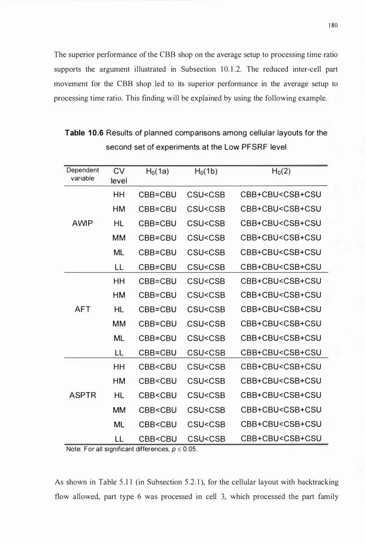
1 80

The superior performance of the eBB shop on the average setup to processing time ratio

supports the argument i l lustrated in Subsection 1 0. 1 .2 . The reduced inter-cell part

movement for the eBB shop led to its superior performance in the average setup to

processing time ratio. This finding wil l be explained by using the fol lowing example.

Table 1 0.6 Results of planned comparisons among cel lu lar layouts for the

second set of experiments at the Low PFSRF level

Dependent CV Ho( 1 a) Ho( 1 b) Ho(2) variable level

H H CBB=CBU CSU<CSB CBB+CBU<CSB+CSU

H M CBB=CBU CSU<CSB CBB+CBU<CSB+CSU

AWI P HL CBB=CBU CSU<CSB CBB+CBU<CSB+CSU

M M CBB=CBU CSU<CSB CBB+CBU<CSB+CSU

ML CBB=CBU CSU<CSB CBB+CB U<CSB+CSU

LL CBB=CBU CSU<CSB C BB+CB U<CSB+CSU

H H CBB=CBU CSU<CSB CBB+CBU<CSB+CSU

H M CBB=CBU CSU<CSB CBB+CBU<CSB+CSU

AFT HL CBB=CBU CSU<CSB CBB+CBU<CSB+CSU

M M CBB=CBU CSU<CSB CBB+CBU<CSB+CSU

ML CBB=CBU CSU<CSB CBB+CBU<CSB+CSU

LL CBB=CBU CSU<CSB CBB+CBU<CSB+CSU

H H CBB<CBU CSU<CSB CBB+CBU<CSB+CSU

H M CBB<CBU CSU<CSB CBB+CBU<CSB+CSU

ASPTR HL CBB<CBU CSU<CSB CBB+CBU<CSB+CSU

MM CBB<CBU CSU<CSB CBB+CBU<CSB+CSU

ML CBB<CBU CSU<CSB CBB+CBU<CSB+CSU

LL CBB<CBU CSU<CSB CBB+CBU<CSB+CSU Note: For al l sign ificant differences, p � 0 .05.

As shown in Table 5 . 1 1 (in Subsection 5 .2 . 1 ), for the cellular layout with backtracking

flow allowed, part type 6 was processed in cell 3, which processed the part family

1 8 1

consisting of five part types, namely : 5 , 6, 1 5 , 1 6, 1 8 . On the other hand, As shown in

Table 5 . 1 8 ( in Subsection 5 .2 .2), for the cellular layout with unidirectional flow, part

type 6 had to be processed in cell 1 first, and then transported to cell 2 for other

operations. The part fami ly processed by cell 1 consisted of part types 5, 6, 1 1 , 1 5 , 1 6

and the part family processed by cell 2 consisted of part types 1 , 2, 3 , 4, 6, 1 0. Therefore,

for the cellular layout with backtracking flow allowed, part type 6 had chances to be

queued with other four part types ( i .e . part types 5, 1 5 , 1 6, 1 8) at the workstations of cell

3 . However, for the cel lular layout with unidirectional flow, part type 6 might be queued

with four other part types ( i .e . part types 5, 1 1 , 5 , 1 6) at the workstations of cell 1 , and

again, with five other part types ( i .e . part types 1 , 2, 3 , 4, 1 0) at the workstations of cell

2 .

S ince more other part types were l ikely to be queued with part type 6 for the cel lular

layout with unidirectional flow, the probabil ity of part type 6 being processed

consecutively by a workstation tended to be lower (Recall that no setup time was

incurred if parts of the same part type were processed consecutively by a workstation).

Consequently, in the long run, the time spent for setting up machines ( or the average

setup to processing time ratio) tended to be longer for the cellular layout with

unidirectional flow.

At the low PFSRF level, the ASPTR performance of the cel lular layout shops tended to

be less constrained by the Part Family Setup Reduction Factor. As a result, the effect of

reduced inter-cel l part movement brought about by intra-cel l backtracking flow became

more significant, and rendered the ASPTR of the CBB shop lower than that of the CBU

shop.

However, at the low level of the Part Family Setup Reduction Factor, the adverse effects

of backtracking flow, such as more jumbled production flow and less efficient material

handling (Recall that the setting of the material handl ing speed for backtracking flow

was always low.) also became more significant. Therefore, the advantage of reduced

inter-cell part movement for the CBB shop was somewhat offset by the disadvantage of

1 82

backtracking flow. Consequently, both the cel lular layout shops with batch production

and conveyance (i .e . the CBB and CBU shops) exhibited similar performances on the

average work-in-process inventory and average flow time at all CV levels.

(b) Comparison between the two cellular layout shops with single-unit production and

conveyance [by testing Ho( 1 b)]

The results of testing the hypothesis, Ho( 1 b) show that for the cellular layout shops with

single-unit production and conveyance (i .e . the CSB and CSU shops), the CSU shop

demonstrated consistent superior performance on all dependent variables to that of the

CSB shop. This finding coincides with that found in Subsection 1 0 . 3 . 1 by examining

Figure 1 0 . 3 .

A t the low level of PFSRF, the unfavourable effect of inflexible use of machines for the

cellular layout (Refer to Subsection 8 . 1 .2 (b) for details .) and the disadvantage of less

synchronised operations brought about by single-unit production and conveyance (Refer

to Subsection 8 . 1 . 1 for detai ls .) were substantially improved because of the lower setup

times. Therefore, the potential of unidirectional flow in realising the benefit of single­

unit production and conveyance became more prominent at the low level of PFSRF, and

eventually led to the superior performance of the CSU shop.

(c) Comparison between the cellular layouts with BPC and the cellular layouts with

SUPC [by testing Ho(2)]

The results of testing the hypothesis, Ho(2) indicated that on the average, the cellular

layout shops with batch production and conveyance ( i .e . the CBB and CBU shops)

always outperformed those with single-unit production and conveyance (i .e. the CSB

and CSU shops).

However, as shown in Figure 1 0 .3 , the inferior performance of the cel lular layout shops

with single-unit production and conveyance was mainly due to the poor performance of

1 83

the CBB shop (i .e . the shop with backtracking flow allowed). Actually, the performance

of the CSU shop ( i .e . the shop with unidirectional flow) itself was similar to that of the

CBB and CBU shop. I n addition, the CSU shop even significantly outperformed the

CBB and CBU shops on A WIP and AFT at the ML and LL levels CV. It appears that

the potential of unidirectional intra-cell production flow in achieving the benefit of

single-unit production and conveyance was most effective with low processing time

variability (or coefficient of variation) and medium to low setup time variability.

(d) Comparison between the functional layout and the cellular layouts [by testing Ho(3)]

As shown in Table 1 0.7, the results of testing Ho(3 ) show that the cel lular layout shops

outperformed the functional layout shop on all dependent variables over al l levels of the

Coefficient of Variation. This result agrees with that obtained in Subsection 8 . 3 .2 (d) for

the first set of experiments. Therefore, we are confident that at the low PFSRF level, the

superior performance of the cellular layouts was robust with respect to both material

handl ing speed and the variabil ity (or coefficient of variation) of setup and processing

times.

As i l lustrated in Subsection 8 . 3 .2 (d), the cellular layout shops were able to demonstrate

superior performance because the disadvantage of dedicating the machines in a cell to

the processing of a fami ly of parts was less significant at the low level of the Part

Family Setup Reduction Factor. Therefore, the potential of cellular manufacturing in

achieving lower average work-in-process inventory and average flow time through

larger extent of setup time reduction was fully exploited.

I n this section, we found that cellular layout is more suitable for a job shop environment

with Kanban-based production control when large extent of setup time reduction (i .e.

with low level of PFSRF) is achievable by adopting cellular manufacturing. However,

the production flow patterns to be adopted for the cellular layout depend on the extent of

the variabil ity (or the coefficients of variation) of setup and processing times. The

cellular layout with single-unit production and conveyance is more suitable when the

1 84

processing t ime variabil ity is low and the setup time variabi l ity is medium to low.

However, at other levels of the setup / processing time variability, batch production &

conveyance and single-unit production & conveyance tend to be equally suitable for the

cellular layout.

Table 1 0.7 Results of planned comparisons among the cel lu lar and functional

layouts for the second set of experiments at the Low PFSRF level

Dependent CV Ho(3)

variable level

HH (CBB+CBU)/2<FL

HM (CBB+CBU)/2<FL

AWI P HL (CBB+CBU)/2<FL

MM (CBB+CBU)/2<FL

ML (CBB+CBU)/2<FL

LL (CBB+CBU)/2<FL

HH (CBB+CBU)/2<FL

HM (CBB+CBU)/2<FL

AFT HL (CBB+CBU)/2<FL

MM (CBB+CBU)/2<FL

ML (CBB+CBU)/2<FL

LL (CBB+CBU)/2<FL

HH (CBB+CBU)/2<FL

HM (CBB+CBU)/2<FL

ASPTR HL (CBB+CBU)/2<FL

MM (CBB+CBU)/2<FL

ML (CBB+CBU)/2<FL

LL (CBB+CBU)/2<FL

Note: For a l l s ignificant differences, p :5: 0.05.

1 85

I n addition, if batch production and conveyance is adopted for the cellular layout, the

intra-cel l flow pattern ( i .e . unidirectional flow or backtracking flow allowed) does not

cause any significant difference in the shop performance (in terms of average work-in­

process inventory and average flow time). On the other hand, if single-unit production

and conveyance is adopted for the cellular layout, unidirectional intra-cel l production

flow should be adopted to achieve better shop performance.

The results and analyses of the simulation output for the second set of experiments have

been discussed in this chapter. The effect of changing the CV level on the performance

of a Kanban-control led job shop was investigated for the different levels of the Shop

Layout and Part Fami ly Setup Reduction Factor variables.

In general, the influence of the variabil ity (of coefficients of variation) of setup and

processing times on the performances of individual layouts was more important than on

their relative performances. The performances of the cellular layout shops with batch

production and conveyance and the functional layout shop were more l ikely to be

affected by the variabi l ity of setup times. For the cellular layout shops with single-unit

production and conveyance, the performance of the shop with backtracking flow

al lowed was more l ikely to be affected by the processing time variabi lity, while both

setup and processing time variability had significant influence on the performance of the

shop with unidirectional flow.

Some similarities regarding the effect of the Part Family Setup Reduction Factor (or the

extent of setup time reduction achievable through cellular manufacturing) were found in

both the first and second sets of experiments. The results of both sets of experiments

indicated that functional layout is more suitable for a Kanban-control led job shop when

only a small extent of setup time reduction ( i .e . high PFSRF level) can be achieved

through cellular manufacturing. On the other hand, if a large extent of setup time

reduction ( i .e . low PFSRF level) is achievable through cellular manufacturing, cellular

layout should be adopted for a Kanban-control led job shop. However, when medium

extent of setup time reduction (i .e . medium level of PFSRF) is achievable through

1 86

cellular manufacturing, both material handling speed and variabil ity of setup and

processing times will affect the choice of the shop layout adopted.

The findings regarding the effects of the four independent variables ( i .e . Shop layout,

Part Family Setup Reduction Factor, Material Handling Speed and Coefficient of

Variation) from both the two sets of experiments will be concluded in Chapter 1 1 .

CHAPTER 1 1

CONCLUSIONS

1 87

I n comparison with other manufacturing environments, the production efficiency of job

shop manufacturing tends to be lower because of its characteristics of low and irregular

volume of demand, high product variety and complex product routings. As depicted in

Section 1 .2 , several Just-in-Time (JIT) manufacturing techniques, such as cellular

manufacturing, single-unit production and conveyance (SUpe), Kanban-based

production control and efficient material handl ing, are very often suggested as effective

tools for reforming job shop manufacturing. However, though there have been abundant

reports on Kanban-based systems, far fewer efforts have been devoted to the study of

the issues related to applying the Kanban-based production control in a job shop

environment. Therefore, how and to what extent those suggested J IT techniques can

affect the performance of job shop manufacturing was not wel l explored. As a result,

inadequate understanding of how a job shop with Kanban-based production control

behaves under different shop conditions and configurations has discouraged

manufacturers from adopting not only the Kanban method but also other effective lIT

techniques in j ob shop environments.

Through this study, we have successfully investigated the influence of several essential

factors on the performance of job shop manufacturing with Kanban-based production

control , and obtained more understanding of the behaviour of a typical Kanban­

controlled j ob shop under various shop conditions and configurations. Several important

findings revealed through this study wil l serve as useful guidelines for manufacturing

firms intending to adopt those suggested JIT tools in job shop environments with

Kanbans.

I n this study, the fol lowing four essential influential factors affecting the performance of

a Kanban-control led job shop were identified :

shop layout / production flow patterns (represented by Shop Layout or SL),

1 88

material handling speed (MHS),

variabi lity of setup and processing times (represented by Coefficient of Variation or

CV), and

extent of setup time reduction achievable through cellular manufacturing

( represented by Part Family Setup Reduction Factor or PFSRF).

To investigate the effects of these factors on the shop performance, two sets of

simulation experiments with different levels of the above influential factors were carried

out, and the effects of the influential factors were identified through statistical analyses

of the simulation outputs. The effects of these influential factors wil l be individually

concluded as follows.

1 1 . 1 Effect of Shop Layout and Production Flow Patterns

In the experimental design of this study, shop layout and production flow patterns were

hncorporated into the different levels of a single independent variable, Shop Layout (See

Section 6 . 1 ). Three basic shop layouts were investigated, namely : the functional layout,

the cel lular layout with backtracking flow allowed and the cellular layout with

unidirectional flow. Each of the two basic cellular layouts was further distinguished

between the one with batch production and conveyance (BPC) and the one with single­

unit production and conveyance (SUPC).

The effect of shop layout and production flow patterns can be considered in three

aspects:

- differences between the cellular layout and the functional layout,

- differences between the cellular layouts with unidirectional flow and those with

backtracking flow allowed, and

- difference between the cellular layouts with single-unit production and conveyance

and those with batch production and conveyance.

1 89

Furthermore, the extent of setup time reduction achievable through cellular

manufacturing was found to have substantial interactions with other influential factors.

In other words, the extent of setup time reduction achievable through cellular

manufacturing affected not only the dependent variables, but also the effects of other

influential factors. Therefore, the effect of shop layout and production flow patterns wil l

be summarised for each of the three aspects, at the different extents of setup time

reduction achievable through cellular manufacturing (i .e . different levels of the Part

Family Setup Reduction Factor) in the fol lowing subsections.

1 1 . 1 . 1 Comparison between the cellular layout and the functional layout

The comparison between the cellular and functional layouts is summarised in Table 1 1 . 1 .

The results show that cellular manufacturing was, as expected, capable of capitalising

on the similarities among the operational sequences of parts to achieve setup time

reduction and resulted in lower average setup to processing time ratios (ASPTR).

However, the potential of cellular manufacturing in improving the average work-in­

process inventory (A WIP) and average flow time (AFT) of the Kanban-control led job

shop was found to be substantially dependent on the extent of setup time reduction

achievable through converting functional layout into cellular layout (i .e . the part family

setup reduction factor).

Table 1 1 . 1 Summary of the comparison between the cel lu lar and

functional layouts

Setup time Amount of setup time reduction achievable through cellular manufacturinq

variabi l ity smal l med ium large

high F = C

low F C C

Note: 1 . The comparison is based on AWI P and AFT. 2 . The entries are defined as follows:

'F ' : Functional layout is more suitable. 'C ' : Cellular layout is more su itable. ' = ' : Both layouts are suitable.

1 90

When the extent of setup time reduction achievable through cellular manufacturing was

small ( i .e . at the high PFSRF level), the inflexibility of dedicating machines to

processing part families caused the performance of the cellular layout shops to be

inferior to that of the functional layout shop (See Subsection 8 . 1 .2 (b)) . I n addition, the

flexibility brought about by interchangeable machines in functional departments and

setup time reduction through the queue selection heuristic rendered the functional layout

superior to the cellular layouts.

When medium extent of setup time reduction could be achieved through adopting

cellular manufacturing (i .e . at the medium PFSRF level), the potential of cellular

manufacturing in setup time reduction was able to greatly overcome its disadvantage of

inflexible use of machines and made the performance of the cellular layout shops

similar, or even superior at some occasions, to that of the functional layout shop.

Provided more efficient material handling facil ities were employed (Refer to Section

9.4.) , a medium to low setup time variability is more l ikely to justify the adoption of

cellular manufacturing in a Kanban-control led job shop; otherwise, the performances for

cellular and functional layouts are similar.

When a large setup time reduction was achievable though the adoption of cel lular

manufacturing (i .e . at the low PFSRF level), the cellular layout was always superior to

the functional layout regardless of the levels of material handling speed and variability

of setup and processing times. The performance of the cellular layout shops was

superior because the unfavourable effect of dedicated use of machines for cellular

manufacturing was less significant and the potential of cel lular manufacturing in setup

time reduction was fully exploited at this level of PFSRF.

This conclusion agrees with the conclusion made by Suresh ( 1 992) that for a given lot

size, setup reduction through converting a functional to a cel lular system must be above

a certain threshold value before a cellular manufacturing system would outperform a

corresponding functional system. Agarwal et al. ( 1 995) extended the study by Suresh

( 1 992) and further confirmed that there exists a region of the combinations of mean

1 9 1

setup to processmg time ratios and setup time values where both the cellular

manufacturing system and the functional system can outperform each other depending

upon the level of setup time reduction and lot size values.

1 1 . 1 .2 Comparison between the cellular layouts with unidirectional flow and those with

backtracking flow allowed

For the cellular layout shops with batch production and conveyance, the relative

performances between the shop with backtracking flow allowed ( i .e . the CBB shop) and

the shop with unidirectional flow ( i .e. the CBU shop) was more susceptible to the

material handling speed than to the variability of setup and processing times. The

comparison between the CBB and CBU shops at the different material handl ing speed

levels is summarised in Table 1 1 .2 .

Table 1 1 .2 Summary of the comparison between the cel lu lar layouts with batch

production and conveyance

Material handl ing Amount of setup time reduction achievable through

speed for cellular manufacturing

inter-cel l i ntra-cel l smal l med ium large

h igh high B = =

high low B B =

low high B = =

low low = = =

Note: 1 . The comparison is based on AWI P and AFT. 2. The entries are defined as follows:

'8 ' : The layout with backtracking flow allowed is more suitable. ' = ' : 80th layouts are su itable.

With a small setup time reduction achievable through cel lular manufacturing ( i .e. the

high PFSRF), the high inter-cell or intra-cell material handling speed resulted in lower

average flow time and average setup to processing time ratios for the CBB shop. The

performances of the CBB and CBU shops on average work-in-process inventory were

similar regardless of the material handling speed levels (Refer to Subsection 8 . 1 .2 (a)) .

1 92

However, when the extent of setup time reduction achievable through cellular

manufacturing became larger, the influence of material handling speed tended to be less

significant and the performances of the two cellular layout shops with batch production

and conveyance tended to be similar in terms of average work-in-process inventory and

average flow time (Refer to Subsections 8 .2 .2 (a) and 8 . 3 .2 (a)).

When the extent of setup time reduction achievable through cellular manufacturing was

small , the eBB shop outperformed the eBU shop for most levels of the variability of

setup and processing times, provided more efficient material handling facilities were

employed. This was due to the disadvantage of increased queue length brought about by

the more intensive inter-cell part movement of the cellular layout with unidirectional

flow (Refer to 1 0 . 1 .2 (a)).

However, when the extent of setup time reduction through cellular manufacturing was

increased to medium or large, the superior performance of the shop with backtracking

flow al lowed was somewhat offset by the more significant disadvantage of backtracking

flow. As a result, the performances of the two cellular layout shops tended to be similar

in terms of average work-in-process inventory and average flow time (Refer to

Subsections 1 0 .2 .2 (a) and 1 0. 3 . 2 (a)) .

Among the cellular layout shops with single-unit production and conveyance, the shop

with unidirectional flow (i .e . the esu shop) always demonstrated superior performance

to that of the shop with backtracking flow allowed ( i .e . the eSB shop) when a medium

to large extent of setup time reduction was achievable through cellular manufacturing

(i .e . at the medium and low levels of PFSRF). This finding suggests that unidirectional

intra-cell production flow was essential for realising the benefit of adopting single-unit

production and conveyance in a job shop environment with Kanban-based production

control . Furthermore, since the same finding was derived from both the first and second

sets of experiments, we are confident that the favourable effect of unidirectional flow

was robust with respect to material handling speed and the variabil ity of setup /

processing times (Refer to Subsections 8 .2 . 1 , 8 .3 . 1 , 1 0.2 . 1 and 1 0. 3 . 1 ).

1 93

I t appeared that the adverse effects of less synchronised operations on shop

performances caused by single-unit production and conveyance could be alleviated by

the smoother and more synchronised production flow resulted from unidirectional intra­

cell production flow. This finding agrees with the conclusion made by Kelleher ( 1 986)

that balanced (synchronised) operations were essential for achieving the benefit of

single-unit production and conveyance in a job shop environment.

1 1 . 1 .3 Comparison between the cellular layouts with SUPC and those with BPC

An important finding from this study, which is contradictory to the view point held by

several lIT proponents, is that single-unit production and conveyance (SUPC) is not

necessarily superior to batch production and conveyance (BPC) in a Kanban-control led

job shop environment. Our findings show that the cellular layout shops with batch

production and conveyance were superior to those with single-unit production and

conveyance on most occasions.

However, it is worth noting that the cel lular layout shops with single-unit production

and conveyance demonstrated much better performance when the extent of setup time

reduction achievable through cellular manufacturing was large ( i .e . at the low level of

PFSRF), particularly for the shop with unidirectional flow (i .e . the CSU shop).

With a large setup time reduction achievable through cellular manufacturing, the CSU

shop even outperformed the cellular layout shops with batch production and conveyance

with low intra-cel l material handling speed, or with low processing time variability and

medium to low setup time variabi lity (provided more efficient material handling

faci lities were employed) (Refer to Subsections 8 .3 . 1 and 1 0 .3 . 1 ) .

The conclusion in this subsection suggest that in a job shop environment with Kanban­

based production control, such shop conditions with large setup time reduction

achievable through cellular manufacturing, unidirectional intra-cel l production flow,

low intra-cel l material handling speed, low processing time variabi l ity and medium to

1 94

low setup time variabi l ity are more likely to justify the adoption of single-unit

production and conveyance.

11.2 Effect of M aterial Handling Speed

As i l lustrated in Chapter 8, the effect of material handl ing speed on the performances (in

terms of average work-in-process inventory and average flow time) of individual shops

with different layouts and production flow patterns was found to be not important.

However, the relative performances among the different shops were affected by material

handling speed, though the effect of material handl ing speed was not as substantial as

that of other influential factors. Table 1 1 . 3 summarises the effect of material handl ing

speed on the relative shop performance.

Table 1 1 .3 Summary of the effects of material handl ing speed on the

relative shop performance

Difference investigated Amount of setup time reduction achievable through

cellular manufacturing

small medium large

functional layout vs. A cel lu lar layout

backtracking flow allowed vs. AR* R unidirectional flow

batch production & conveyance vs. A single-unit production &conveyance

* The entry for a specific d ifference investigated at a specific level of setup time reduction is defined as follows: 'AR' : The effects of both intra- and inter-cel l material handl ing speeds are important. 'A' : The effect of intra-cel l material handling speed is important. ' R ' : The effect of inter-cell material handling speed is important. blank: The effect of material handling speed is not important.

Since material handling speed also had some interactions with the extent of setup time

reduction achievable through cellular manufacturing, the effect of material handling

speed wil l be summarised for the different extents of setup time reduction achievable

through cellular manufacturing in the following subsections.

1 95

1 1 .2 . 1 Conclusions for the high PFSRF level

With only a small setup time reduction achievable through cellular manufacturing (i .e .

at the high PFSRF level), higher ( inter-cel l or intra-cell) material handl ing speed

resulted in both lower average flow time and average setup to processing time ratios for

the cellular layout shop with BPC and backtracking flow allowed (i .e . the CBB shop)

than the cel lular layout shop with BPC and unidirectional flow (i .e. the CBU shop)

(Refer to Subsection 8 . 1 .2 (a)).

However, as concluded in Subsection 1 1 . 1 . 1 , at the high PFSRF level, because of the

disadvantage of inflexible use of machines, the performance of the cellular layout shops

was inferior to that of the functional layout shop regardless of the influence of material

handling speed.

1 1 .2 .2 Conclusions for the medium PFSRF level

When a medium setup time reduction was achievable through cellular manufacturing

( i .e . at the medium level of PFSRF), the influence of material handl ing speed on the

relative performance of the cellular layout shops with batch production and conveyance

was lessened. Only the higher inter-cell material handling speed resulted in lower

average flow time and average setup to processing ratios of the CBB shop (Refer to

Subsection 8 .2 .2 (a)).

In addition, at the medium level of PFSRF, the relative performance between the

cellular layouts and the functional layout was somewhat affected by material handling

speed. The cel lular layout shops outperformed the functional layout shop, except that

lower intra-cell material handling speed rendered the average work-in-process inventory

of the cel lular layout shops similar to that of the functional layout shop. Therefore,

although cel lular layout was found to be more suitable for a Kanban-control led job shop

at the medium PFSRF level, faster material handling faci lities for intra-cel l part

movement should be employed to achieve better shop performance (Refer to Subsection

8 .2 .2 (c)).

1 96

1 1 .2 .3 Conclusions for the low PFSRF level

When a large setup time reduction could be achieved by adopting cellular

manufacturing (i .e . at the low PFSRF level), material handling speed mainly affects the

relative performance between the cellular layout shops with BPC and the cellular layout

shops with SUPC. When the intra-cel l material handling speed was low, the cellular

layout with SUPC and unidirectional flow was found to be more suitable for a Kanban­

control led job shop; otherwise, the cellular layout with batch production and

conveyance should be adopted.

I n general , the effect of material handling did not substantially affect the decision on the

shop layout and production flow patterns to be adopted for a Kanban-control led job

shop. To achieve better production performance in a job shop environment with

Kanban-based production control, it is more important to select the correct shop layout

and production flow patterns based on the extent of setup time reduction achievable

through cellular manufacturing. Once the shop layout and production flow patterns are

decided, proper material handling faci lities can then be selected based the above

conclusions to achieve better shop performance.

1 1 .3 Effect for the Variability of Setup and Processing Times

As il lustrated in Chapter 1 0, in contrast to the effect of material handling speed, the

influence of the variabi lity (or coefficients of variation) of setup and processing times

was mainly on the individual performances of the different shops instead of their

relative performances. The effect of setup / processing time variabil ity on the individual

shop performances is summarised in Table 1 1 .4 .

Similar to the findings for the other influential factors, the variabil ity of setup and

processing times was also found to have substantial interactions with the extent of setup

time reduction achievable through cellular manufacturing (or the Part Family Setup

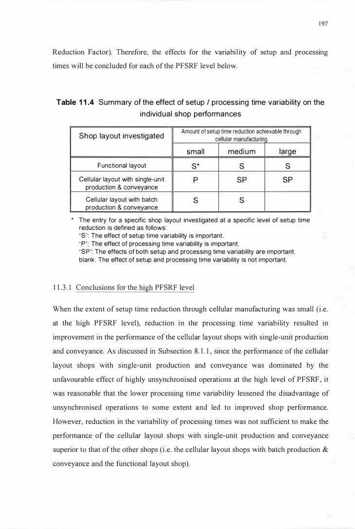
1 97

Reduction Factor). Therefore, the effects for the variabi l ity of setup and processing

times wil l be concluded for each of the PFSRF level below.

Table 1 1 .4 Summary of the effect of setup / processing time variabi l ity on the

individual shop performances

Shop layout investigated Amount of setup time reduction achievable through

cellular manufacturing

smal l med ium large

Functional layout S* S S

Cel lu lar layout with single-un it p SP SP production & conveyance

Cel lu lar layout with batch S S production & conveyance

* The entry for a specific shop layout investigated at a specific level of setup time reduction is defined as follows: '8 ' : The effect of setup time variability is important. ' P ' : The effect of processing time variabil ity is important. '8P' : The effects of both setup and processing time variability are important. blank: The effect of setup and processing time variabil ity is not important.

1 1 .3 . 1 Conclusions for the high PFSRF level

When the extent of setup time reduction through cellular manufacturing was small ( i .e .

at the high PFSRF level), reduction in the processing time variabi lity resulted in

improvement in the performance of the cellular layout shops with single-unit production

and conveyance. As discussed in Subsection 8 . 1 . 1 , since the performance of the cellular

layout shops with single-unit production and conveyance was dominated by the

unfavourable effect of highly unsynchronised operations at the high level of PFSRF, it

was reasonable that the lower processing time variabil ity lessened the disadvantage of

unsynchronised operations to some extent and led to improved shop performance.

However, reduction in the variabil i ty of processing times was not sufficient to make the

performance of the cellular layout shops with single-unit production and conveyance

superior to that of the other shops ( i .e . the cellular layout shops with batch production &

conveyance and the functional layout shop).

1 98

On the other hand, for the remaining shops, the influence of setup time variability on

their performances was more important. Because the performances of these shops were

mainly confined by the longer setup times at the high level of PFSRF, the lower setup

time variabi l ity was effective in reducing the unfavourable effect of longer setup times

and leading to better shop performances (Refer to Subsection 8 . 1 . 1 ) .

The effect of setup and processing time variabi l ity on the relative performance between

the various shops was not significant at this level of PFSRF. In addition, as concluded in

Subsection 1 1 . 1 . 1 , at the high PFSRF level, because of the disadvantage of inflexible

use of machines, the performance of the cellular layout shops were i nferior to that of the

functional layout shop regardless of the influence of setup and processing time

variabil ity.

1 1 .3 .2 Conclusions for the medium PFSRF level

If medium extent of setup time reduction could be achieved through adopting cellular

manufacturing ( i .e . at the medium level of PFSRF), the effect of the variability of setup

and processing times was the same as that for the high PFSRF level, except that

reducing setup time variabi l ity became more effective in improving the performance of

the cel lular layout shop with single-unit production & conveyance and unidirectional

flow (i .e . the CSU shop) (Refer to Subsection 8 .2 . 1 ) . However, because of the

disadvantage of less synchronised operations (Refer to Subsection 8 . 1 . 1 ), the

performance of the cellular layout shops with single-unit production and conveyance

was stil l inferior to that of other shops.

At the medium PFSRF level, the setup time variabi lity had significant effect on the

relative performance between the functional layout shop and the cel lular layout shops.

Provided more efficient material handl ing facil ities were employed, the cellular layout

shops (with batch production and conveyance) outperformed the functional layout shop

(in terms of average work-in-process inventory and average flow time) with medium to

low setup time variabil ity. Otherwise, their performances on average work-in-process

inventory and average flow time were similar (Refer to 1 0 .2 .2 (c)) .

1 99

1 1 .3 .3 Conclusions for the low PFSRF level

When a large setup time reduction was achievable by adopting cel lular manufacturing,

reduction in the variabil ity of both setup and processing times significantly improved

the performance (in terms of average work-in-process inventory and average flow time)

of the cellular layout shop with single-unit production & conveyance and unidirectional

flow (i .e . the CSU shop). Furthermore, the CSU shop outperformed all other shops (in

terms of average work-in-process inventory and average flow time) with low processing

time variabil ity and medium to low setup time variability (Refer to Subsection 1 0.3 . l ) .

Similar to the findings for the high and medium levels of PFSRF, reduction in the setup

time variability resulted i n lower average work-in-process inventory and average flow

time for the functional layout. However, in contrast to the findings for the high and

medium PFSRF levels, the influence of setup and processing t ime variabi lity on the

performance of the cellular layout shops with batch production and conveyance was not

significant (Refer to Subsection 1 0 . 3 . l ) .

No significant effect of the setup and processmg time variability on the relative

performance of the various shops could be found. As concluded in Subsection 1 1 . 1 . 1 , at

the medium PFSRF level, the cellular layout shops outperformed the functional layout

shop regardless of the influence of setup and processing time variability.

Similar to the conclusion for the effect of material handling speed in Section 1 1 .2 , the

effect of setup and processing variability did not substantially affect the decision on the

shop layout and production flow patterns to be adopted for a Kanban-control led job

shop. We found that the selection of shop layout and production flow patterns based on

the extent of setup time reduction achievable through cellular manufacturing was

essential for achieving better production performance in a job shop environment with

Kanban-based production control . Once the shop layout and production flow patterns

are decided, reduction of setup and / or processing time variabi lity should then be

considered to improve the shop performance by referring to the above conclusions.

200

1 1 .4 Effect for the Extent of Setup Time Reduction Achievable through Cellular

Manufacturing

Several proponents of lIT manufacturing (Monden 1 983 : 67, Kelleher 1 986,

Schonberger 1 986: 9 and Cheng and Podolsky 1 993) emphasised that converting the

traditional functional layout into cel lular layout was essential for reforming job shop

manufacturing. However, through this study, we found that converting functional layout

into cellular layout does not necessarily bring about improved shop performance in a job

shop environment with Kanban-based production control .

Our finding agrees with that reported by Suresh ( 1 992) and Agarwal ( 1 995), who

concluded that for a given lot size, setup time reduction through converting a functional

layout to a cellular layout must be above a certain threshold before a cellular

manufacturing system would outperform a corresponding functional system. In addition,

we found that the extent of setup time reduction achievable through cellular

manufacturing not only had a significant effect on the performance of a Kanban­

control led job shop, but also had significant interactions with other influential factors

(as concluded in the previous sections for the individual influential factors).

The findings from our study show that cellular layout is more suitable for a Kanban­

control led job shop when a medium to large setup time reduction can be achieved by

adopting cellular manufacturing, provided more efficient material handling facilities are

adopted. Otherwise, functional layout should be adopted for a Kanban-control led job

shop if the extent of setup reduction achievable by adopting cellular manufacturing is

small .

The extent of setup time reduction achievable through cellular manufacturing, shop

layout and production flow patterns together were the most essential factors which

influenced the production performance in a job shop environment with Kanban-based

production control . We found that to successfully implement the Kanban mechanism in

a job shop, it is essential to select the correct shop layout and production flow patterns

20 )

(i .e. batch production & conveyance vs. single-unit production & conveyance, and

unidirectional flow vs. backtracking flow allowed) according to what extent of setup

time reduction can be achieved by adopting cellular manufacturing (as concluded in

Section 1 1 . 1 ). In addition, when planning the shop layout, the cell formation and layout

planning procedures (as i llustrated in Sections 5 .2-4) should be fol lowed to properly

position cells / departments on the available floor area.

Once the shop layout and production flow patterns are decided, attention should be

given to the selection of appropriate material handling faci lities (as concluded in Section

1 1 .2) and the reduction of setup / processing time variabil ity (as concluded in Section

1 1 . 3 ) to attain better shop performance.

From this research project, we realise that implementation of the lust-in-Time

techniques in a job shop environment is not as simple as grouping machines into cells or

putting Kanban cards in the shop. The benefits of those lIT related tools (e.g. Kanban­

based production control, cellular manufacturing, single-unit production and

conveyance) cannot be realised without taking into account the effects of those

influential factors investigated in this study. We believe that the conclusions in this

chapter as well as the content in other chapters wil l provide valuable information for

manufacturing firms to successfully implement lIT techniques in job shop environments.

In the next chapter, we wil l give the managerial implications derived from the

conclusions, and our recommendations for both industrial applications and future

research work.

202

CHAPTER 1 2

MANAGERIAL I MPLICATIONS AND RECOMMENDATIONS

In this chapter, important managerial implications wil l be derived from the conclusions

of this study. They wil l serve as practical guidelines for those manufacturers who wish

to implement Just-i n-Time manufacturing techniques in job shop environments. Then

recommendations for industrial applications and future research work wil l be given.

1 2 . 1 Managerial Implications

From the conclusions of this study, we are able to arrive at the following managerial

implications:

( 1 ) The selection of an appropriate shop layout and production flow patterns based on

the extent of setup time reduction achievable through cellular manufacturing should

be given the first priority in the design and planning of the Kanban-based

production control system in a job shop environment. I n practice, the case studies

by Gunasekaran and Lyu ( 1 997) and Martin-Vega et al. ( 1 989) emphasised the

importance of layout planning in realising the benefits of Kanban-based systems as

wel l .

I n a job shop environment with Kanbans, the traditional functional layout is more

appropriate if only small amount of setup time reduction can be achieved by

adopting cel lular manufacturing (Refer to Subsections 1 1 . 1 . 1 , 8 . 1 .2(b) and

1 O . 1 .2(b )) . The use of cellular layout should only be considered when a medium to

large setup time reduction is achievable by adopting cellular manufacturing (Refer

to Subsections 1 1 . 1 . 1 , 8 .2 .2(c), 8 . 3 .2(d), 1 0 .2 .2(c) and I O. 3 .2(d» .

(2) The method of single-unit production and conveyance is more appropriate for

repetitive manufacturing. In a job shop environment, where parts require quite

different routings, the adoption of single-unit production and conveyance should

203

only be considered when setup time can be reduced significantly by adopting

cellular manufacturing and where intra-cell material handl ing facil ities with lower

speed (e.g. workers) are used (Refer to Subsection 8 . 1 . 1 ) .

Furthermore, if single-unit production and conveyance is to be implemented,

unidirectional intra-cel l production flow should be used, and the variability of both

setup and processing times must be significantly reduced. (Refer to Subsections

1 1 . 1 .2, 1 1 . 1 .3 , 8 .3 . 1 and 1 0. 3 . 1 ) .

(3) As opposed to single-unit production and conveyance, the method of batch

production and conveyance is more suitable for a job shop environment with

Kanban-based production control when a small to medium setup time reduction is

achievable through cel lular manufacturing (Refer to Subsections 1 1 . 1 .3 , 8 . 1 . 1 , I

8.2 .2(b), 1 0 . 1 . 1 and 1 0.2 .2(b)). I n addition, one important advantage of batch

production and conveyance is that it is more robust with respect to the influence of

the i ntra-cell production flow pattern ( i .e . unidirectional flow vs. backtracking flow

allowed) than single-unit production and conveyance. (Refer to Subsections 1 1 . 1 .2,

8 . 1 .2(a) , 8 .2 .2(a), 1 O . 1 .2(a) and 1 0 .2.2(a)).

(4) As concluded in Section 1 1 .2 , as long as the shop layout and production flow

patterns are properly selected, and material handl ing facilities with reasonable speed

are used, the effectiveness of employing faster material handl ing methods in

increasing the performance of a Kanban-control led job shop is l imited. Therefore, to

achieve the benefits of using Kanbans in a job shop environment, layout changes

should always be given the higher priority than investment in faster (or more

advanced) material handl ing facil ities.

(5) As i l lustrated in Section 1 1 .3 and Chapter 1 0, reducing the variabi l ity of setup /

processing times is effective in achieving higher productivity in a job shop

environment with Kanbans. The study by Philipoom et al. ( 1 987) also highlighted

the importance of reducing processing time variabi lity in achieving better

performance of a job shop with Kanbans. However, it should not be ignored that the

204

effectiveness of reducing setup / processing time variability varies for shops with

different layouts and production flow patterns .

Reduction in the variability of both setup and processmg times is effective in

improving the performance of the cel lular layout with single-unit production &

conveyance and unidirectional flow (Note that the use of single-unit production and

conveyance should only be considered when a large setup time reduction is

achievable through cellular manufacturing). However, for the functional layout and

the cellular layout with batch production & conveyance, reduction in the variability

of setup times should be given the higher priority (The use of the cel lular layout

with single-unit production & conveyance and backtracking flow al lowed is not

recommended).

Reduction in the variabi lity of setup/processing times can be achieved by

implementing standard operations. The implementation of the standard operations

involves preparing standard operating charts, training workers to fol low standard

operations and continuous improvement of operations (Shingo 1 989: 1 4 1 - 1 48).

(6) The issue of improving the production performance of job shop manufacturing by

adopting TIT techniques is particularly important for the manufacturing firms in

New Zealand. Because of the relatively much smaller market in New Zealand than

in other more industrialised countries, such as U.S . , U.K. and Japan, manufacturers

often have to adopt the job shop manufacturing approach. However, with the high

manpower cost in New Zealand, it is essential for job shop manufacturers to

improve their production performance if they want to remain competitive in the

market.

Some typical New Zealand industries where the results of this study can be applied

include: communication equipment where the variabil ity of the demand is high,

automation / control products (PLCs, Inverters, etc .), sheet metal products

(equipment racks, cabinets, heat sinks, etc. ), metal / machining products (tube

fittings, connectors, etc .), and process instruments (pressure gauges, thermometers,

flowmeters, valves, etc.) .

205

1 2.2 Recommendations for Industrial Applications

Through this research project, we have gained invaluable knowledge of the

requirements and approaches for realising the potential of Just-in-Time manufacturing

in improving the production performance in a job shop environment. Based on our

experience in conducting the simulation experiments and the results obtained from the

study, we have the fol lowing recommendations deserving attention for industrial

applications.

1 2 .2 . 1 Vulnerabi lity of the Kanban-based systems to disturbances

A Kanban-based production control system is more vulnerable to disturbances (e.g. less

synchronised operations, variabil ity in setup / processing times, etc . ) than traditional

systems without Kanbans. Any fluctuation in part of the system can be easily

transmitted (and even amplified) to the entire system (Kimura and Terada 1 98 1 , Villeda

et al. 1 988) .

More Kanban / container sets are needed to buffer production fluctuations if

disturbances happen too often. Eventual ly, the advantages of using the Kanban for

continuous improvement (e.g. reducing work-in-process inventory) wil l be lost with

larger numbers of Kanbans and containers. Therefore, a crucial prerequisite for

successful implementation of the Kanban method is that manufacturers should

endeavour to bring the disturbances down to a minimum in any case (Monden 1 983 : 26-

28, Cheng and Podolsky 1 993 : 85-88).

1 2 .2 .2 Incorporating the planning of cellular manufacturing in TQM activities

The findings of our study support the effectiveness of cellular manufacturing In

improving the performance of job shop manufacturing with Kanban-based production

control , provided the shop layout and production flow patterns are properly selected

(Refer to Subsection 1 1 . 1 . 1 , Sections 8 .2-3 and Sections 1 0.2-3) . However, we would

like to emphasise, that implementing cellular manufacturing is not as simple as merely

grouping machines into cells.

206

As pointed out by Vakharia and Selim ( 1 994), the introduction of cellular

manufacturing will affect the existing structure, personnel, methods, and procedures of a

plant. Some issues, l ike stabilisation of end product demand, activity-based costing

systems, changes in the structural configuration of the operations function, team

atmosphere within each cell and support of top management will also need to be

resolved. These issues are all the aspects addressed by Total Quality Management

(TQM). We thus strongly suggest that the planning for cellular manufacturing be

introduced as part of the company-wide TQM activities.

1 2 .2 .3 Using simulation and statistical methods correctly

When planning a Kanban-based system, it is important to evaluate the feasibility of

system parameters and configurations. If the system is a new one, it is impossible to

carry out such feasibil ity studies on a real system. Even where an existing system is

available, the required interruptions and modifications to the existing system for

performing such studies can be costly, if not impossible.

As shown in this study, simulation in conjunction with statistical methods is an effective,

yet inexpensive decision support tool for evaluating the expected system performance at

the planning and design stages. For example, in our study, each simulation run had to

simulate about fourteen years (43 ,080 working hours) of the production activities to

achieve the appropriate statistical reliabi l ity in the results. This job can never be

accomplished on a real system, but it can be done by simulation in about three hours.

Simulation is particularly useful when the system is too complicated to be studied by

other modell ing methods, such as the analytical method, the empirical method, etc. ; or

characterised by stochastic properties, which can be easily incorporated in a simulation

model.

We would like to point out, however, improper use of simulation and statistical methods

can lead to wrong decisions. For example, if the initial transient period of a simulation

run is simply determined by assumption or even ignored, as had done in many

simulation studies, the effect of initial transient may substantial ly bias the simulation

results. Another example is that interpreting the simulation results based merely on the

207

mean values of dependent variables (again, as had done in many simulation studies)

without investigating their confidence intervals can lead to totally different conclusions.

To achieve correct simulation results and to interpret the simulation results correctly, the

fol lowing issues deserve attention in performing a simulation experiment (Refer to

Chapter 7 for details) :

( 1 ) A simulation model should be systematical ly verified after it is developed and

coded to make sure the model functions as expected.

(2) If the purpose of a simulation study is to examine the system's steady-state

behaviour, the statistics col lected during the initial transient period must be

discarded to avoid the simulation results being biased. The initial transient period of

a simulation run should be determined through a valid procedure, such as the

Welch's graphical procedure (Law and Kelton 1 99 1 , p. 545) instead of by

assumption.

(3) As shown in Equation 7 .3 , the number of replications, n ( i .e . the simulation run

length) of a simulation run is directly related to how precisely the confidence

interval of the population mean can be estimated. The larger the number of

replications, the smaller is the error in estimating the population mean (i .e . The

confidence interval is narrower). To achieve an acceptable confidence interval for

the population mean, an appropriate number of replications should be decided by

performing preliminary simulation runs before the commencement of a full

simulation experiment. An experimenter wil l risk making wrong decisions based on

simulation results with large errors if the number of replications of a simulation is

not determined appropriately.

(4) To interpret the simulation results correctly, we suggest that the confidence

intervals of population means or suitable hypothesis tests be used for comparing the

sample means of different treatment groups. If the confidence intervals had not

been shown on the bar graphs of Figures 8. 1 -3 and 1 0. 1 -3 , the interpretation of the

208

simulation results would be substantial ly different. As shown in the discussions of

Chapters 8 and 1 0, comparing two treatment groups solely by their sample means is

only appropriate when there is no overlap between their confidence intervals for

population means.

1 2.3 Recom mendations for Future Research Work

This research project has made a significant advance in the area of applying Just-in­

Time (lIT) manufacturing techniques in the job shop environment. The effects of

several influential factors on the production performance in a job shop environment

with Kanbans were investigated, and many important findings were revealed. However,

for J IT manufacturing techniques to be widely accepted in job shop environments as

they are for repetitive manufacturing, further understanding of how to apply these

techniques effectively for job shop manufacturing is sti l l needed. Therefore, we would

l ike to suggest the fol lowing directions for future research work in this area.

1 2 . 3 . 1 Investigating the effects of setup times and the setup to processing time ratio

Agarwal et al. ( 1 995) investigated the behaviour of a cellular layout (CL) shop and a

functional layout (FL) shop as a function of two parameters: the mean setup time (1) to

processing time (t) ratio (denoted by R=Tlt) and the mean setup time.

They identified five distinct regions within the defined ranges of the two parameters

where: ( 1 ) the CL and FL shops were both unstable, (2) the FL shop always

outperformed the CL shop, (3) the CL shop always outperformed the FL shop

(consisting of two regions) and (4) the CL and FL shops could outperform each other (a

mixed region) depending on the amount of setup time reduction achievable by adopting

cellular manufacturing (or the part family setup reduction factor), and lot size values.

In this study, the R and the T values were defined as constants lying in the ' mixed

region' so that the influence of the part family setup reduction factor could be

209

investigated. However, in consideration of the findings by Agarwal et al. , varying the R

and T values may affect the production performance in a job shop environment with

Kanban-based production control as wel l . In addition, the influence of material handl ing

speed may be different with different R and T values.

Therefore, extending this study by investigating the influence of R and T values on the

production performance of a Kanban-control1ed job shop is a potential area for future

research work.

1 2 . 3 .2 I nvestigating the influence of setup time reduction by improving setup

operations

As concluded in Section 1 1 .4, the amount of setup time reduction achievable through

cellular manufacturing (or the part family setup reduction factor) had a substantial effect

on the performance of job shop manufacturing with Kanbans. However, in addition to

setup time reduction achieved by adopting cel lular manufacturing, substantial setup time

reduction is also achievable by improving setup operations. Shingo ( 1 985) suggested

that an average of setup time reduction around 80 to 95 percent is achievable by

improving setup operations, such as preparation of material, clamping and removing

dies and tools, centring and determining dimensions of tool ing, and trial processing and

adjustment.

Therefore, another subject deserving further study is the examination of how and to

what extent the amount of setup time reduction achieved by improving setup operations

affect the production performance in a job shop environment with Kanban-based

production control .

1 2 . 3 . 3 Assessing the importance of influential factors using fractional factorial design

As i l lustrated in Sections 6 . 1 and 9.2, the full factorial design was adopted for both the

two sets of experiments for this study. The strength of the full factorial design is that

complete information regarding the main and interaction effects of the factors

2 1 0

investigated can be obtained. However, as the number o f factors increases, the number

of runs required by a full factorial design increases geometrically. For example, for our

project, each set of experiments required 5 x 3 x 6 = 90 runs. I f we add another factor

with three levels, the number of runs required will increase to 5 x 3 x 6 x 3 = 270. In

addition, as the number of factors increases, an increasing portion of the data for the full

factorial design is used to estimate higher-order interactions. These interactions are

often of l ittle interest to the experimenter (Moen et al. 1 99 1 ).

Therefore, if we use the full factorial design to investigate the effects of all the relevant

factors (included in this study and recommended in previous subsections) for future

research work, the size of experiments wil l become extremely large and interpretation of

the interaction effects wil l be very complicated. In this case, fractional factorial designs

are more suitable. Fractional factorial designs enable the estimation of important effects

while keeping the size of experiments practical .

We suggest that a set of experiments with the fractional factorial design or screening

experiments such as the Plackett Burman design are performed first to identify the

importance of all the relevant factors with fewer levels. Based on the information gained

from these experiments, factors with important main effects and / or interactions can be

identified. Then, experiments with the ful l factorial design can be conducted to obtain

detailed information on the effects and interactions of those important factors.

S ince the emergence of the Just-in-Time manufacturing in late 1 973 in Japan, TIT has

been recognised globally as one of the most important tools for increasing the

productivity of manufacturing plants. In general, JIT is not as easily applied to job shop

manufacturing as to repetitive and continuous manufacturing. This study should

stimulate the awareness of the problems as wel l as the benefits of using TIT

manufacturing techniques in job shop environments.

More research effort is sti l l needed to understand all the issues related to the

implementation of J IT manufacturing techniques m job shop environments.

2 1 1

Understanding of the requirements for realising the benefits of lIT manufacturing

techniques wil l eventually help job shop manufacturing firms to implement these

techniques more correctly and more effectively.

2 1 2

REFERENCES

Agarwal, A., Huq, F. and Sarkis, J., 1 995, "Performance of manufacturing cells for

group technology: a parametric analysis". In : Kamrani , A. K. and others (Ed.),

Planning, Design, and Analysis of Cellular Manufacturing System (Amsterdam:

Elsevier Science), p. 1 67- 1 80.

Apple, J . M., 1 963, Plant Layout and Materials Handling (2nd ed.) (New York: The

Roland Press Company).

Apple, 1. M., 1 972, Material Handling Systems Design (New York: The Roland Press

Company).

Burbidge, 1 . L., 1 989, Production Flow Analysis for Planning Group Technology

(Oxford: Clarendon Press).

Cheng, T. C. E. and Podolsky, S., 1 993, Just-in-Time Manufacturing: An Introduction

(London: Chapman & Hall).

Emmons, H., Flowers, A. D., Khot, C . M. and Mathur, K., 1 992, STORM Personal

Version 3. 0: Quantitative Modelling for Decision Support (Englewood Cliffs, NJ:

Prentice Hall / Al lyn & Bacon).

Emshoff J . R. and Sisson, R. L., 1 970, Design and Use of Computer Simulation Models

(New York: The Macmillan Company) .

Esparrago, Jr . , R. A. , 1 988, "Kanban", Production and Inventory Management, Vol . 29,

No. 1 : 6- 1 0 .

F lynn, B . B . , 1 987, " Repetitive lots the use of a sequence-dependent set-up time

scheduling procedure in group technology and traditional shops", Journal of

Operations Management, Vol . 7, No. 1 &2 : 203-2 1 6.

2 1 3

Flynn, B . B . and Jacobs, F . R., 1 987, "An experimental comparison of cellular (group

technology) layout with process layout", Decision Sciences, Vo!. 1 8 , No.4: 562-

58 1 .

Gravel, M. and Price, W., 1 988, "Using the Kanban in a job shop environment",

International Journal of Production Research, Vo!. 26, No.6: 1 1 05- 1 1 1 8 .

Grunwald, H . , Striekwold, P. E . T. and Weeda, P . J . , 1 989, "A framework for

quantitative comparison of production control concepts", International Journal of

Production Research, Vo!. 27, No.2 : 28 1 -292.

Gunasekaran, A. and Lyu, 1 . , 1 997, "Implementation ofjust-in-time in a small company :

a case study", Production Planning and Control, Vo!. 8, No. 4 : 406-4 1 2 .

I rani , S . A. and Ramakrishnan, R., 1 995, "Production flow analysis using STORM". In :

Karnrani , A. K. and others (ed.), Planning, Design, and Analysis of Cellular

Manufacturing Systems (Amsterdam: Elsevier Science), p . 299-349.

Kimura, O . and Terada, H. , 1 98 1 , "Design and analysis of pull system, a method of

multi-stage production control", International Journal of Production Research,

Vo!. 1 9, No. 3 : 24 1 -253 .

Kelleher, J . P . , 1 986, "HT application in the job shop environment", APICS Conference

Proceedings: 348-35 1 .

Law, A. M . and Kelton, W. D . , 1 99 1 , Simulation Modeling and Analysis (New York:

McGraw-Hil l ) .

Li , J-W. and Nahavandi, S . , 1 997, "Information flow model for HT shopfloor control

systems", Proceedings of the International Symposium on Manufacturing Systems

(ISMS '97), World Manufacturing Congress (WMC97), 1 8-2 1 November,

Auckland: 1 8 1 - 1 87.

L indman, H. R. , 1 992, Analysis of Variance in Experimental Design (New York:

Spring-Verlag) .

2 1 4

Lee, C . -Y. , Lin, c.-S . , Uzsoy, R. and Wong, c.-C. , 1 994, "Implementation of a

demand-pull system in a job shop environment", International Journal of

Production Research, Vol. 32, No. 1 2 : 291 5 -2927.

Mahmoodi F., Dooley, K. 1 . and Starr, P . J., 1 990, "An investigation of dynamic group

scheduling heuristics in a job shop manufacturing cell", International Journal of

Production Research, Vol. 29, No. 9 : 1 695- 1 7 1 1 .

Martin-Vega, L . A. , Pippin, M. , Gerdon, E. and Burcham, R., 1 989, "Applying just-in­

time in a wafer fab: a case study", IEEE Transactions on Semiconductor

Manufacturing, Vol . 2, No. 1 : 1 6-22.

Moen, R. D., Nolan, T. W. and Provost, L. P. , 1 99 1 , Improving Quality through

Planned Experimentation (Boston, MA: McGraw-Hil l ) .

Monden, Y., 1 983, Toyota Production System (Atlanta: Industrial Engineering and

Management Press).

Morris, 1. S. and Tersine, R. J., 1 990, "A simulation analysis of factors influencing the

attractiveness of group technology cellular layouts", Management Science, Vol. 36,

No. 1 2 : 1 567- 1 578 .

Muther, R., 1 973, Systematic Layout Planning (Boston: Cahners Books}.

Nakamura, M. , Sakakibara, S . and Schroeder, R., 1 998, "Adoption of Just-in-Time

manufacturing methods at U.S . - and Japanese-owned plants : some empirical

evidence", IEEE Transactions on Engineering Management, Vol. 45, No. 3 : 230-

235 .

Phi lipoom, P . R . , Rees, L. P . , Taylor I l l , B . W. and Huang, P. Y . , 1 987, "An

investigation of the factors influencing the number of Kanbans required in the

implementation of the J IT technique with Kanbans", International Journal of

Production Research, Vol . 25, No. 3 : 457-472.

Russell, E . c., 1 990, Building Simulation Models with SIMSRIPT 11. 5 (La Jolla, CA:

CACI Products Company).

2 1 5

Sandras, B . , 1 985, "Job shop lIT", APICS Conference Proceedings: 448-452 .

Schonberger, R . J . , 1 986, World Class Manufacturing: The Lessons of Simplicity

Applied (New York: The Free Press).

Shingo, S . , 1 985, A Revolution in Manufacturing: The SMED System (Cambridge, M.

A. , Productivity Press).

Shingo, S . , 1 989, A Study of the Toyota Production System from an Industrial

Engineering Viewpoint (Cambridge, M . A . : Productivity Press).

Sornrnervil le, I . , 1 996, Software Engineering 5th ed.(Wokingham, England: Addison­

Wesley Publ ishing Company).

South, J. B . , 1 986, "A minimum production lot-size formula for stockless production",

Production and Inventory Management, Vol. 27, No. 2 : 1 43 - 1 50.

Stockton, D. 1 . and Lindley, R. 1 . , 1 995, "Implementing kanbans within high

variety/low volume manufacturing environments", International Journal of

Operations and Production Management, Vol . 1 5 , No. 7 : 47-59.

Suresh, N. C., 1 992, "Partitioning work centers for group technology: Analytical

extension and shop-level simulation investigation", Decision Sciences, Vol. 23, No.

2: 267-290.

Vakharia, A. J. and Selim, H. M., 1 994, "Group technology". In: Dorf, R C. and Kusiak,

A. (ed.) , Handbook of Design, Manufacturing and Automation (New York: John

Wiley and Sons), p. 435-460.

Vakharia, A. 1 . and Wernrnerl6v, U., 1 990, "Designing a cellular manufacturing system:

a material flow approach based on operation sequences", 11E Transactions, Vol . 22,

No. 1 : 84-97.

Villeda, R, Dudek, R. and Smith M. L., 1 988, "Increasing the production rate of a j ust­

in-time production system with variable operation times", International Journal of

Production Research, Vol. 26, No. 1 1 : 1 749- 1 768.

2 1 6

Vollmann, T. E . , Berry, W. L . and Whybark, D . c. , 1 992, Manufacturing Planning and

Control Systems, 3rd ed. (Homewood, I L : Business One Irwin).

Wemmerlov, U and Hyer, N . L . , 1 989, "Cellular manufacturing in the US. industry : A

survey of users", International Journal of Production Research, Vol. 27, No. 9 :

1 5 1 1 - 1 530.

Yavuz, I . H . and Satir, A., 1 995, "A kanban-based simulation study of a mixed model

j ust-in-time manufacturing l ine", International Journal of Production Research,

Vol. 3 3 , No. 4 : 1 027- 1 048.

ApPENDIX 1 FROM-To CHARTS FOR THE V ARIOUS SHOP LAYOUTS

Table A 1 . 1 From-to chart for the cel lu lar layout with u nid i rectional flow

un it: batches per year From To (Cel l) (Cel l)

I n 1 2 3 4 5 Out

.

1 382 1 057 1 568 1 1 49 I n --

1 -- 362 291 729

2 -- 304 1 264

3 -- 1 859

4 -- 1 1 49

5 1 49 -- 1 304

Out* --

21 7

Table A 1 .2 From-to chart for the cel lu lar layout with backtracking flow al lowed

un it: batches per year

From To (Cel l)

(Cel l) I n 1 2 3 4 Out

I n -- 1 1 1 5 1 1 55 2 1 79 764

1 -- 1 1 1 5

2 -- 1 1 55

3 -- 291 1 888

4 -- 1 055

Out --

From (Dept. )

I n

I n --

1 - --.. -

2

3

4

5 ----.-.-.

6

7

8

9 -'--

1 0

1 1 ",._-

1 2

Out

-- --- -- ------

2 1 8

Table A 1 .3 From-to chart for the functional layout

un it: batches per year

To (Dept.)

1 2 3 4 5 6 7 8 9 1 0 1 1 1 2 Out

2862 1 060 269 2502 1 207 96

-- 640 978 698 546 -......... -- . __ ._ ........ H ....... •• _ __ •• OH._

-- 640 51 5

-- 1 060

-- 1 492 2327

5 1 5 -- 545 . __ ._._-_ .. -. .. _ ..... _ ... _.- -_ ... ..... H ................ .. . .. _-_. _ ... _ ......... _-.. H ........ __ ......... H • .. _ .. _ ... --_ .

1 393 - - 1 1 66 1 222 479

539 -- 1 1 64 1 01 1 1 763 546 387 270

270 -- 2952 269

-- 3963 --_.

. __

.. -

f---'----f--- . . - - _._-- --

1 222 -- 546 1 763

984 546 -- 769 ____ .H ••• __ _ .M .. _.H ............ ..................... _ .. -_ .. _ ... _ ..... " .......... __ . __ . ._ ............ _-_. H •••••••

-- 1252

--

2 1 9

ApPENDIX 2

FLOW-OF-MATERIAL INTENSITIES FOR THE VARIOUS SHOP LAYOUTS

Table A2.1 Flow-of-material intensity for the cel lu lar layout with

unid irectional flow

Between Pair of Cells Flow-of-Material Importance of I ntensity Relationship

(batches per year) Rating

3 Out 1 859 1 *

In 3 1 568 1

In 1 1 382 2

5 Out 1 304 2

2 -- Out 1 264 2

I n 4 1 1 49 3

4 5 1 1 49 3

I n 2 1 057 3

1 Out 729 4

2 -- 5 453 Un important

1 2 362 U nimportant

1 3 291 U nimportant * Note: An importance of relationship rating of ' 1 ' indicates that closeness

between the pair of cells/departments is the most essential . The larger the number of rating is, the less important is the closeness.

Table A2.2 Flow-of-materia l intensity for the cel lu lar layout with

backtracking flow al lowed

Between Pa i r of Cells Flow-of-Material Importance of I ntensity Relationship

(batches per year) Rating

I n -- 3 2 1 79 1

3 -- Out 1 888 1

I n -- 2 1 1 55 3

2 -- Out 1 1 55 3

I n -- 1 1 1 1 5 3

1 -- Out 1 1 1 5 3

4 -- Out 1 055 3

I n -- 4 764 4

3 -- 4 291 Un important

220

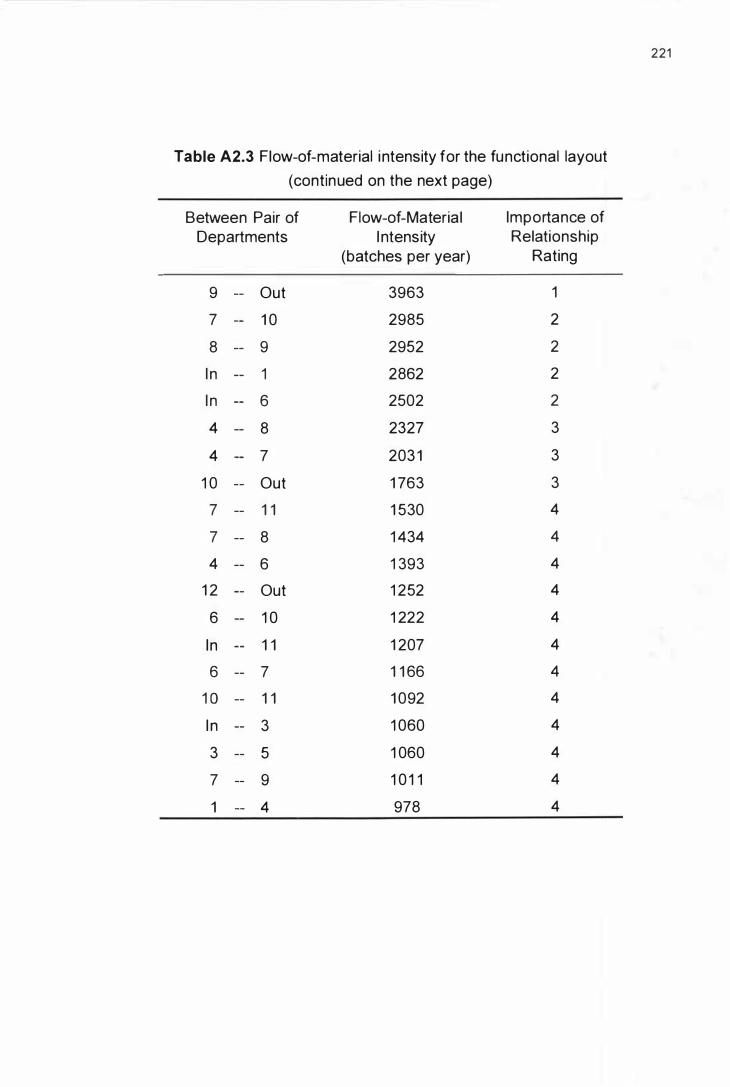
221

Table A2.3 Flow-of-material i ntensity for the functional layout

(continued on the next page)

Between Pair of Flow-of-Materia l Importance of Departments I ntensity Relationship

(batches per year) Rating

9 -- Out 3963 1

7 -- 1 0 2985 2

8 -- 9 2952 2

I n -- 1 2862 2

I n -- 6 2502 2

4 -- 8 2327 3

4 -- 7 203 1 3

1 0 -- Out 1 763 3

7 -- 1 1 1 530 4

7 -- 8 1 434 4

4 -- 6 1 393 4

1 2 -- Out 1 252 4

6 -- 1 0 1 222 4

In - - 1 1 1 207 4

6 -- 7 1 1 66 4

1 0 -- 1 1 1 092 4

I n -- 3 1 060 4

3 -- 5 1 060 4

7 -- 9 1 0 1 1 4

1 -- 4 978 4

222

Table A2.3 Flow-of-material i ntensity for the functional layout (contin ued)

Between Pair of Flow-of-Material Importance of Departments I ntensity Relationship

(batches per year) Rating

1 1 -- 1 2 769 U nimportant

1 -- 6 698 Un important

1 -- 2 640 Un important

2 -- 4 640 Un important

1 -- 7 546 Un important

5 -- 6 545 Un important

2 -- 5 5 1 5 Un important

2 6 5 1 5 Un important

6 Out 479 U nimportant

7 -- 1 2 387 U nimportant

7 -- Out 270 Un important

I n -- 4 269 Un important

8 -- Out 269 Un important

I n - - 1 2 96 Un important

APPENDIX 3

FLOW RELATIONSHIP DIAGRAMS FOR THE V ARIOUS SHOP LAYOUTS

LEGEND

W Receiving department

W Shipping department

o Manufacturing cell

Importance of relationship

1 = = = 2 = : : = : : = 3

223

. . . . . . . 4 No connection: unimportant

Figure A3.1 Flow relationship diagram for the cel lu lar layout with

un id i rectiona l flow

LEGEND

\7 Receiving department

W Shipping department

o Manufacturing cell

Importance of relationship

- 1 = = = 2 = : : = : : = 3 . . . 4 No connection: un important

Figure A3.2 Flow relationship diagram for the cel lu lar layout with

backtracking flow al lowed

224

LEGEND

'VI Receiving department Importance of relationship '0/ Shipping department - 1 = : = 2 = : : = ::: 3

0/ ( ) Functional depatment . . . . . . . . . . . . 4 No connection: unimportant

....

Figure A3.3 Flow relationship d iagram for the functional layout

225

226

ApPENDIX 4

SPACE RELATIONSHIP DIAGRAMS FOR THE VARIOUS

SHOP LAYOUTS

CELL I

I Q- - , I 1 1

7 1 1

CELL 4 6 2- - -> 1 (OUT)

84' 0"

CELL 3 -l 0 1

� O � I

Shipping Dept.

(") tTl r r Vl

CELL 2 , 7

LEGEND

__ Inter-cell part movement path

Intra-cel l part - -> movement path

with conveyors

C8:J Cel l incoming job storage

Ea el l outgoing job storage

D Machine footprin ( 1 4 ft x I 4 ft)

Figure A4. 1 Space relationship d iagram for the cel lu lar layout with

un id i rectional flow

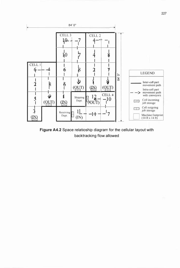
84' 0"

CELL 3

�Q... - -7 1 I I �O �

1 I CELL 1 1 � (j - r- -4 6

I 1 1 I 1 I 1 � J � 6 I 1 (ggT) 1 I I 1 � Shipping

1 (�T) � Dept.

3 Receiving rn 1 L _ � Dept. (IN)

CELL 2

1- I- - I I I 1 1

4 $ 1 1 1 1

1 1 1 1

� � (lli) (9JbT) �, 1� CELL 4 - -10 OUT) 1

I I

-It - _1 7

LEGEND

__ Inter-cell part movement path

Intra-cel l part - -> movement path

with conveyors

C8:J Cell incoming job storage

a::3 Cell outgoing job storage

227

D Machine footprint ( 1 4 f h 1 4 ft)

Figure A4.2 Space relatiosh ip d iagram for the cel lu lar layout with

backtracking flow al lowed

2

·� r · · 1 .. : . ,

84' 0"

70'

0"

228

LEGEN D

Inter-department - part movement

path

Department IZI incoming job

storage

Department Ea outgoing job

n." LJ

storage

Machine footprint ( 1 4 ft x 1 4 ft)

Figure A4.3 Space relationship d iagram for the functional layout

229

ApPENDIX 5

INTER-CELL / DEPARTMENT AND INTRA-CELL TRAVELLING D ISTANCE

MATRICES

Table AS.1 I ntra-cel l d istance matrix for Cell 1 with un id i rectional flow

(material handl ing by a conveyor)

unit: feet

From To Workstation No.lMach ine Type Workstation No.!

Machine type I n 1 /1 2/6 3/1 0 4/7 5/9 Out

I n -- 7 2 1 49 63 77 84

1 /1 -- 1 4 42 56 70 77 M' ___ " ' __ ._---_ .

. -'--

2/6 -- 28 42 56 63

3/1 0 -- 1 4 28 35 --_._- ---f----

4/7 -- 1 4 21

5/9 -- 7 --_ ....... - ............ _ .. _ ....... _-_ .. _ .... _ . . _-_ ...... _ ..... _ ....... -- .. _ .. _ . . _--f----

Out --

Table AS.2 I ntra-cel l d istance matrix for Cell 2 with un id i rectiona l flow

(material handl ing by a conveyor)

unit: feet

From To Workstation No .lMachine Type Workstation No.!

Machine type I n 6/1 7/2 8/4 9/7 1 0/8 1 1 /9 Out

I I n -- t.-�-- 2 1 3 5 49 63 77 84

.. __ ._-- .. _-_._-

6/1 -- 1 4 28 42 56 70 77

7/2 -- 1 4 28 42 56 63 ... _ ... _-- ........ .... _ ...... _-_. __ ... .. _._--- ---

8/4 -- 1 4 28 42 49

9/7 -- 1 4 28 35 --- ---f----..

1 0/8 -- 1 4 2 1

1 1 /9 I -- 7 ........... _------- --- ----l

Out I --

230

Table A5.3 I ntra-cel l d istance matrix for Cell 3 with un id i rectional flow

(material hand l ing by a conveyor)

From To Workstation No.lMach ine Type Workstation No.!

Machine type I n 1 2/1 1 1 3/6 1 4/7 1 5/1 0 1 6/1 1 1 7/1 2 Out

I n

--t-

2 1 42 56 77 9 1 98 . _-- 1------- ..

1 2/1 1 -- 1 4 35 49 70 84 9 1

1 3/6 -- 2 1 35 56 70 77

1 4/7 -- 1 4 35 49 56

1 5/1 0 -- 2 1 3 5 42 ..... __ . __ . - ----f----.. --.... - ---_.-

1 6/1 1 -- 1 4 2 1

1 7/1 2 -- 7

Out - -

231

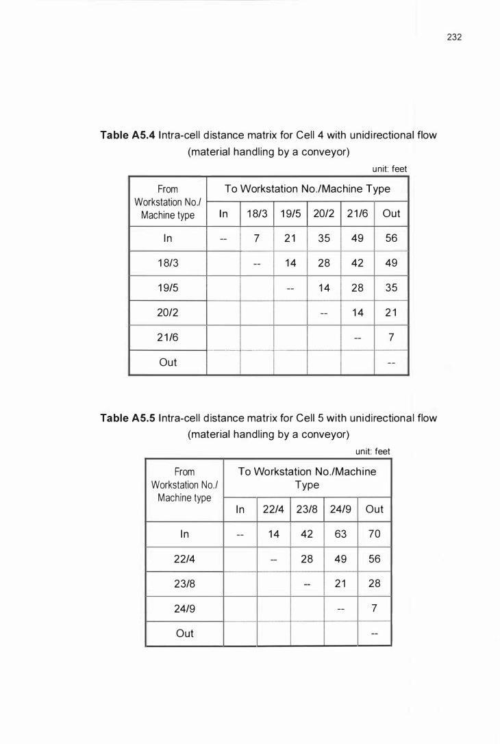
Table AS.4 I ntra-cel l d istance matrix for Cell 4 with un id i rectional flow

(material handl ing by a conveyor)

unit: feet

From To Workstation No .lMachine Type Workstation No.!

Machine type I n 1 8/3 1 9/5 20/2 2 1 /6 Out

I n -- 7 2 1 35 49 56

1 8/3 -- 1 4 28 42 49

1 9/5 -- 1 4 28 35

20/2 -- 1 4 2 1

2 1 /6 -- 7 ---_ .. --- ._._.

Out - -

Table AS.S I ntra-cel l d istance matrix for Cel l 5 with un id i rectiona l flow

(material handl ing by a conveyor)

un it: feet

From To Workstation No.lMach ine Workstation No.! Type

Machine type I n 22/4 23/8 24/9 Out

I n -- 1 4 42 63 70

22/4 -- 28 49 56

23/8 -- 2 1 28

24/9 -- 7

Out --

232

Table AS.S I ntra-cel l d istance matrix for Cell 1 with un id i rectional flow

(manual materia l handl ing)

un it : feet

From To Workstation No.lMach ine Type Workstation No.!

Machine type I n 1 /1 2/6 3/1 0 4/7 5/9 Out

I n -- 7 35 49 35 2 1 --

1 /1 -- 28 42 28 1 4 2 1

2/6 -- 28 1 4 28 35

3/1 0 -- 28 42 49

4/7 -- 28 35

5/9 -- 7

Out --

Table AS.7 I ntra-cel l d istance matrix for Cell 2 with un id i rectional flow

(manual materia l handl ing)

unit: feet

From To Workstation No.lMach ine Type Workstation No .!

Machine type I n 6/1 7/2 8/4 9/7 1 0/8 1 1 /9 Out

I n -- 7 35 49 49 35 2 1 --

6/1 -- 28 42 42 28 1 4 2 1

7/2 -- 28 28 1 4 28 35

8/4 -- 1 4 28 42 49

9/7 -- 28 42 49

1 0/8 -- 28 35

1 1 /9 -- 7

Out --

233

Table A5.8 I ntra-cel l d istance matrix for Cell 3 with un id i rectional flow

(manual materia l handl ing)

un it: feet

From To Workstation No.lMach ine Type Workstation No.!

Machine type I n 1 2/1 1 1 3/6 1 4/7 1 5/1 0 1 6/1 1 1 7/1 2 Out

I n -- 7 35 56 56 35 21 --

1 2/1 1 -- -- 28 49 49 28 1 4 2 1

1 3/6 -- -- -- 35 35 1 4 28 35

1 417 -- -- -- -- 1 4 35 49 56

1 5/1 0 -- -- -- -- -- 35 49 70

1 6/1 1 -- - - -- - - -- -- 28 35

1 7/1 2 -- -- -- -- -- - - -- 7

Out - - -- -- -- -- -- -- --

Table A5.9 I ntra-cell d istance matrix for Cell 4 with un id i rectional flow

(manual material hand l ing)

unit: feet

From To Workstation No.lMachine Type Workstation No.!

Machine type I n 1 8/3 1 9/5 20/2 2 1 /6 Out

I n -- 7 35 35 21 --

1 8/3 -- 28 28 1 4 2 1

1 9/5 -- 1 4 28 35

20/2 -- 28 35

2 1 /6

-+

7 '--'-'--'--- ._ ............... _ ... _ .... ...... __ ._-- ..........

Out - -

234

235

Table AS. 1 0 I ntra-cel l d istance matrix for Cell 5 with un id i rectional flow

(manual materia l hand l ing)

unit: feet

From To Workstation No .lMachine Workstation No.! Type

Machine type I n 22/4 23/8 24/9 Out

I n -- 1 4 42 35 --

22/4 -- 28 28 2 1 _.-

23/8 -- 2 1 28

24/9 -- 7

Out --

Table AS. 1 1 I ntra-cel l d istance matrix for Cell 1 with backtracking flow al lowed

(material handl ing by a conveyor)

un it: feet

From To Workstation No.lMach ine Type Workstation No.!

Machine type I n 1 /3 2/5 3/2 4/6 5/4 6/8 7/9 Out

I n -- 7 2 1 35 49 63 77 9 1 --

1 /3 -- 1 4 28 42 56 70 84 9 1

2/5 28 -- 1 4 28 42 56 70 77

3/2 42 28 -- 1 4 28 42 56 63

4/6 56 42 28 -- 1 4 28 42 49

5/4 56 42 28 1 4 -- 1 4 28 35

6/8 42 28 1 4 28 28 -- 1 4 2 1

7/9 28 1 4 28 42 42 28 - - 7 ___ 0. .-

Out --

236

Table A5. 1 2 I ntra-cel l d istance matrix for Cell 2 with backtracking flow al lowed

(material handl ing by a conveyor)

unit: feet

From To Workstation No.lMach ine Type Workstation No.!

Machine type I n 8/1 9/2 1 0/4 1 1 /8 1 2/7 1 3/9 Out

I n -- 7 2 1 42 77 9 1 1 05 --

8/1 - - - - 1 4 35 70 84 98 1 05

9/2 -- 28 -- 2 1 56 70 84 9 1 ---

1 0/4 -- 49 35 -- 35 49 63 70

1 1 /8 -- 42 28 2 1 -- 1 4 28 35

1 2/7 -- 28 1 4 35 28 -- 1 4 2 1

1 3/9 -- 1 4 28 49 42 28 -- 7

Out --

237

Table A5.1 3 I ntra-cel l d istance matrix for Cell 3 with backtracking flow al lowed

(material handl ing by a conveyor)

unit: feet

From To Workstation No.lMachine Type Workstation No.!

Machine type I n 1 4/1 1 5/6 1 6/1 0 1 7/7 1 8/8 1 9/9 Out

I n -- 7 28 56 70 9 1 1 05 --

1 4/1 -- 2 1 49 63 84 98 1 05

1 5/6 35 -- 28 42 63 77 84 • __ .H ••••••••••••••• H •• __ ._ ._._._-_.- ___ • __ •••••• H .... _. ___ H. ___ _ •• __ •• H ••

1 6/1 0 63 42 -- 1 4 35 49 56

1 7/7 63 42 1 4 -- 2 1 35 42

1 8/8 42 2 1 35 35 -- 1 4 2 1

1 9/9 28 2 1 49 49 28 -- 7

Out --

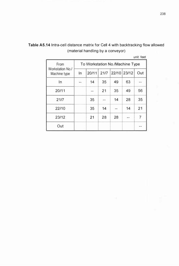
238

Table AS.1 4 I ntra-cel l d istance matrix for Cell 4 with backtracking flow al lowed

(material hand l ing by a conveyor)

unit: feet

From To Workstation No.lMach ine Type Workstation No.!

Machine type I n 20/1 1 2 1 /7 22/1 0 23/1 2 Out

I n -- 1 4 35 49 63 --

20/1 1 -- 2 1 35 49 56

2 1 /7 35 -- 1 4 28 35

22/1 0 35 1 4 -- 1 4 2 1

23/1 2 21 28 28 - - 7 ----" " ".

Out - -

239

Table A5.1 5 I ntra-cel l d istance matrix for Cell 1 with backtracking flow al lowed

(manual materia l handl ing)

unit: feet

From To Workstation No./Mach ine Type Workstation No.!

Mach ine type I n 1 /3 2/5 3/2 4/6 5/4 6/8 7/9 Out

I n -- 7 35 49 63 63 49 35 --

1 /3 -- 28 42 56 56 42 28 2 1

2/5 28 -- 28 42 42 28 1 4 2 1

3/2 42 28 -- 28 28 1 4 28 35

4/6 56 42 28 - - 1 4 28 42 49 ._ ......... .. _-_ . . __ ...... _.

5/4 56 42 28 1 4 -- 28 42 49

6/8 42 28 1 4 28 28 -- 28 35

7/9 28 1 4 28 42 42 28 -- 7

Out --

240

Table A5. 1 6 I ntra-cel l d istance matrix for Cell 2 with backtracking flow al lowed

(manual material handl ing)

un it: feet

From To Workstation No.lMach ine Type Workstation No.!

Machi ne type I n 8/1 9/2 1 0/4 1 1 /8 1 2/7 1 3/9 Out

I n -- I 7 35 56 49 35 21 --

8/1 -- 28 49 42 28 1 4 2 1

9/2 28 -- 35 28 1 4 28 35

1 0/4 49 35 -- 2 1 3 5 49 56 .. ----- _ ..

1 1 /8 42 28 21 -- 28 42 49

1 2/7 28 1 4 35 28 -- 28 35

6/9 1 4 28 49 42 28 -- 7

Out --

241

Table A5. 1 7 I ntra-cel l d istance matrix for Cel l 3 with backtracking flow al lowed

(manual material handl ing)

unit: feet

From To Workstation No.lMach ine Type Workstation No.!

Machine type I n 1 4/1 1 5/6 1 6/1 0 1 7/7 1 8/8 1 9/9 Out

I n -- 7 42 70 70 49 35 --

1 4/1 -- 35 63 63 42 28 21

1 5/6 35 -- 42 42 2 1 2 1 28

1 6/1 0 63 42 -- 1 4 35 49 56

1 7/7 63 42 1 4 -- 35 49 56

1 8/8 42 2 1 35 35 -- 28 35

1 9/9 28 2 1 49 49 28 -- 7

Out --

242

Table A5. 1 8 I ntra-cel l d istance matrix for Cell 4 with backtracking flow al lowed

(manual material handl ing)

un it: feet

From To Workstation No.lMach ine Type Workstation No.!

Machine type I n 20/1 1 2 1 /7 22/1 0 23/1 2 Out

I n -- 28 49 49 35 --

20/1 1 -- 35 35 21 2 1

2 1 /7 35 -- 1 4 28 35

22/1 0 35 1 4 -- 28 35

23/1 2 2 1 28 28 -- 7

Out I --

Table A5. 1 9 I nter-cel l d istance matrix for the cel lu lar layout with

un id i rectional flow

unit: feet

From To (Cel l)

(Cel l) I n 1 2 3 4 5 Out

I n -- 2 1 21 7 2 1 49 --�'M' __ .. e.--.. _ �-

1 -- 56 28 42 70 63

2 28 -- 1 4 28 42 35

3 28 28 -- 42 28 21

4 1 4 28 1 4 -- 56 49

5 56 56 42 70 -- 7

Out --

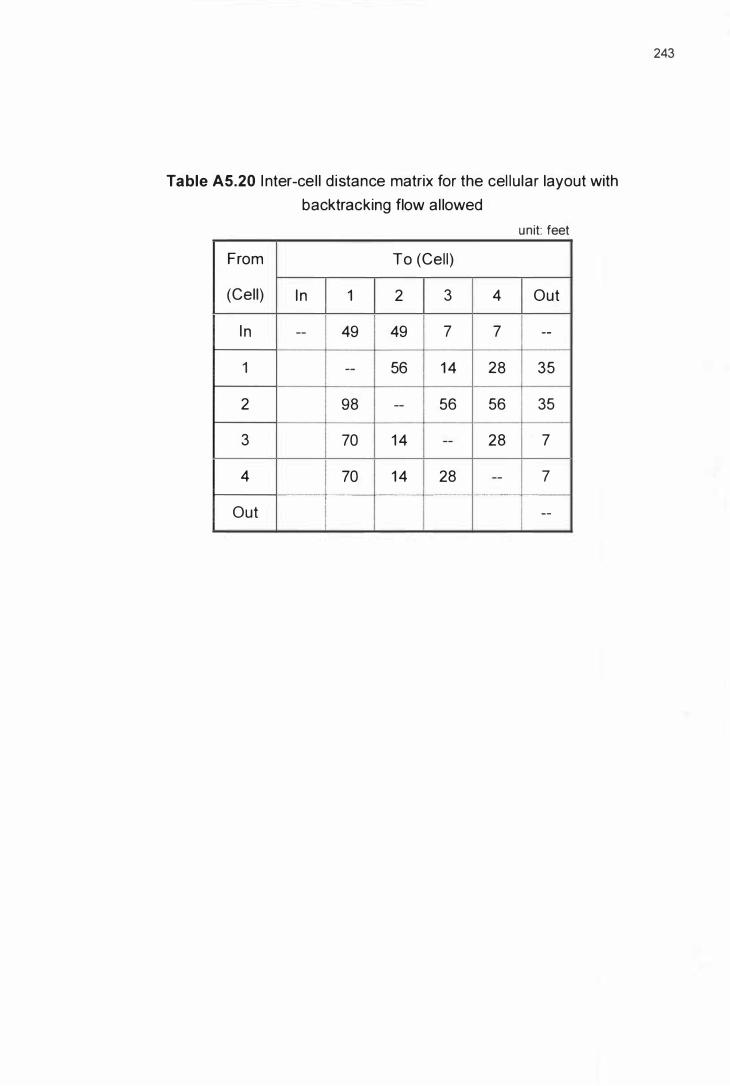
Table AS.20 I nter-cel l d istance matrix for the cel lu lar layout with

backtracking flow al lowed

unit: feet

From To (Cel l)

(Cell) I n 1 2 3 4 Out

I n -- 49 49 7 7 --

1 -- 56 1 4 28 35

2 98 -- 56 56 35

3 70 1 4 -- 28 7

4 I 70 1 4 28 -- 7 ---.. ----t-.--.... -... ---

_'H'_'_" _ _ .... _ ... _ .... _._ .. _ . . _--- _ .. _---

Out I --

243

Table AS.21 I nter-department d istance matrix for the functional layout

un it: feet

From To (Department)

(Dept. ) I n 1 2 3 4 5 6 7 8 9 1 0 1 1 1 2 Out

I n -- 7 49 28 84 42 1 4 28 21 77 56 49 56 --

1 -- -- 70 7 77 21 2 1 35 28 84 63 70 35 77

2 -- 56 -- 77 63 91 49 35 56 84 63 1 4 1 05 91

3 -- 35 91 -- 84 7 42 56 49 49 28 77 1 4 56

4 -- 77 49 84 -- 70 84 42 49 63 42 35 84 56

5 -- 49 1 05 28 70 -- 56 70 63 49 42 91 7 42

6 -- 21 35 42 84 56 -- 28 2 1 77 56 35 70 84 -- _.- --- --_ . . _ ... __ . -_. r-'-'--'

7 -- 35 35 42 56 56 42 -- 2 1 49 28 2 1 70 56

8 -- 42 56 49 63 63 49 21 -- 42 2 1 42 77 49

9 -- 84 98 63 49 49 91 63 70 -- 35 84 35 7

1 0 -- 77 77 56 42 42 84 42 49 7 -- 63 56 1 4

1 1 -- 70 28 77 35 63 63 21 42 56 35 -- 77 63

1 2 -- 63 1 1 9 42 56 28 70 84 77 35 56 1 05 -- 28

Out -- - - -- -- -- -- -- - -- -- -- -- -- --

244

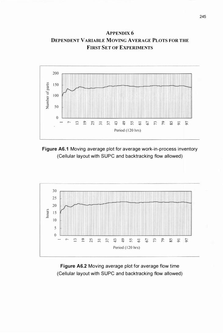
C/l -.... ro 0..

c..-o .... (1) oD E ::l

;z:

APPENDIX 6 DEPENDENT VARIABLE MOVING AVERAGE PLOTS FOR THE

FIRST SET OF EXPERIMENTS

200

1 50

1 00

50

0

Period ( 1 20 hrs)

Figure AS. 1 Moving average plot for average work-in-process inventory

(Cel lu lar layout with SUPC and backtracking flow al lowed)

30

25

20 C/l ....

1 5 ::l 0

..c: 1 0

5

0 - l"- t'"> 0- V") - - N

Period ( 1 20 hrs)

Figure AS.2 Moving average plot for average flow t ime

(Cel lu lar layout with SUPC and backtracking flow al lowed)

245

�

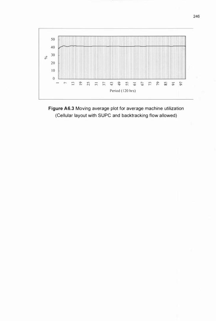
50

40

30

20

1 0

o

Period ( 1 20 hrs)

Figure A6.3 Moving average plot for average machine uti l ization

(Cel lu lar layout with SUPC and backtracking flow a l lowed)

246

ApPENDIX 7 NUMBERS OF INTRA-CELL AND INTER-CELL CONVEYANCE KANBANS

Table A7. 1 Numbers of intra-cel l Kanbans for Cell 1 with

un id i rectional flow and SUPC*

Part Demand Number of Kanbans at

Type ( lots/day) Workstation No.lMach ine type

1 /1 2/6 3/1 0 4/7 5/9

5 1 . 85 3 3 3 3 3

6(a)** 1 . 39 2 2 2

1 1 0 .95 4

1 5(a) 0 .50 5 5

1 6(a) 0 .62 4 4

• single-unit production and conveyance

•• The letter in ' ( ) , indicates the sequence of the cells in which a specific part type was processed.

247

Table A7.2 Numbers of i ntra-cel l Kanbans for Cel l 2 with

un id i rectional flow and SUPC

Part Demand Number of Kanbans at

Type ( lots/day) Workstation No.lMach ine type

6/1 7/2 8/4 9/7 1 0/8 1 1 /9

1 1 .05 3 3 3 3

2(a) 0 .57 5 5 5

2(c) 0 .57 5

3 1 . 1 3 3 3 3 3 3 3

4 0 .71 7 7 7 7

6(b) 1 . 39 2 2

1 0(a) 0.60 6 6

Table A7.3 Numbers of intra-cel l Kanbans for Cell 3 with

un id i rectional flow and SUPC

Part Demand Number of Kanbans at

Type ( lots/day) Workstation No.lMachine type

1 2/1 1 1 3/6 1 4/7 1 5/1 0 1 6/1 1 1 7/1 2

1 2 0.69 1 6 1 6 1 6

1 3 0 .71 1 0 1 0

1 4 0.75 1 9 1 9 1 9

1 5(b) 0 .50 5 5 5 5

1 6(b) 0.62 4 4 4 4

1 7 0 .57 1 5 1 5 1 5

1 8 3 .09 2 2 2

1 9 0 .22 1 4

248

Table A7.4 Numbers of intra-cel l Kanbans for Cell 4 with

un id i rectional flow and SUPC

Part Demand Number of Kanbans at

Type ( lots/day) Workstation No.lMachine type

1 8/3 1 9/5 20/2 2 1 /6

7(a) 0 .88 3

8(a) 1 . 37 3 3 3 3 ..

9(a) 2 . 1 7 2 2 2

Table A7.S Numbers of intra-cel l Kanbans for Cel l 5 with

un id i rectional flow and SUPC

Part Demand Number of Kanbans at

Type ( lots/day) Workstation No.lMachine type

22/4 23/8 24/9

2(b) 0 .57 5 5

7(b) 0 .88 3 3 3 -

8(b) 1 . 37 3 3 3

9(b) 2 . 1 7 2 2 2

1 0(b) 0.60 6 6

249

Table A7.6 Numbers of intra-cel l Kanbans for Cell 1 with

un id i rectional flow and SPC*

Part Demand Number of Kanbans at

Type ( lots/day) Workstation No.lMachine type

1 /1 2/6 3/1 0 4/7 5/9

5 1 . 85 1 2 1 1 1

6(a) 1 . 39 1 1 1

1 1 0 .95 1

1 5(a) 0 .50 1 1

1 6(a) 0 .62 1 1

* batch production and conveyance

Table A7.7 Numbers of intra-cel l Kanbans for Cel l 2 with

un id i rectional flow and SPC

Part Demand N umber of Kanbans at Type (lots/day) Workstation No.lMach ine type

6/1 7/2 8/4 9/7 1 0/8 1 1 /9

1 1 . 05 1 1 1 1

2(a) 0 .57 1 1 1

2(c) 0 .57 1

3 1 . 1 3 1 1 1 1 1 1

4 0 .71 1 1 1 1

6(b) 1 . 39 1 1

1 0(a) 0.60 1 1

250

Table A7.8 Numbers of intra-cel l Kanbans for Cell 3 with

un id i rectional flow and BPC

Part Demand Number of Kanbans at Type ( lots/day) Workstation No.lMach ine type

1 2/1 1 1 3/6 1 4/7 1 5/1 0 1 6/1 1 1 7/1 2

1 2 0 .69 2 1

1 3 0 .7 1 1

1 4 0 .75 2 1 1

1 5(b) 0 .50 1 1 1

1 6(b) 0 .62 1 1 1

1 7 0 .57 1 1

1 8 3 .09 1 1 2

1 9 0 .22

Table A7.9 Numbers of i ntra-cel l Kanbans for Cell 4 with

un id i rectional flow and BPC

Part Demand Number of Kanbans at Type ( lots/day) Workstation No .lMachine type

1 8/3 1 9/5 20/2 2 1 /6

7(a) 0 .88 1

8(a) 1 . 37 1 1 1 1

9(a) 2 . 1 7 1 1 2

2

1

1

1

1

1

251

Table A7. 1 0 Numbers of intra-cel l Kanbans for Cel l 5 with

un id i rectional flow and BPC

Part Demand Number of Kanbans at

Type ( lots/day) Workstation No./Machine type

22/4 23/8 24/9

2(b) 0 .57 1 1

7(b) 0 .88 1 1 1

8(b) 1 . 37 1 1 1

9(b) 2 . 1 7 1 1 2

1 0(b) 0.60 1 1

Table A7. 1 1 Numbers of intra-cel l Kanbans for Cel l 1 with

backtracking flow a l lowed and SUPC

Part Demand Number of Kanbans at Type ( lots/day) Workstation No .lMachine type

1 /3 2/5 3/2 4/6 5/4 6/8 7/9

7 0 .88 3 3 3 3

8 1 .37 3 3 3 3 3 3 3

9 1 . 08 4 4 4 4 4 4

1 1 0 . 95 4

252

Table A7.1 2 Numbers of intra-cel l Kanbans for Cell 2 with

backtracking flow al lowed and SUPC

Part . Demand Number of Kanbans at Type ( lot/day) Workstation No.lMach ine type

8/1 9/2 1 0/4 1 1 /8 1 2/7 1 3/9

1 1 .05 3 3 3 3

2 0.72 4 4 4 4

3 1 . 1 3 3 3 3 3 3 3

4 0 .83 6 6 6 6

1 0 0 .71 5 5 5

Table A7. 1 3 Numbers of intra-cel l Kanbans for Cel l 3 with

backtracking flow al lowed and SUPC

Part Demand Number of Kanbans at Type ( lots/day) Workstation No.lMachine type

1 4/1 1 5/6 1 6/1 0 1 7/7 1 8/8 1 9/9

5 2 .78 2 2 2 2 2

6 1 . 39 2 2 2 2 2 .. -----.

1 5(a) 0 .50 5

1 6(a) 0 .62 4

1 8 3 .09 2 2 2

253

Table A7. 1 4 Numbers of intra-cel l Kanbans for Cel l 4 with

backtracking flow al lowed and S U PC

Part Demand Number of Kanbans at Type ( lots/day) Workstation No .lMach ine type

20/1 1 2 1 /7 22/1 0 23/1 2

1 2 0.69 1 6 1 6 1 6

1 3 0 .7 1 10 1 0 -

1 4 0.75 1 9 1 9 1 9

1 5(b) 0 .50 5 5 5 5

1 6(b) 0 .62 4 4 4 4

1 7 0 .57 1 5 1 5 1 5

1 9 0 .22 1 4

Table A7. 1 5 Numbers of intra-cel l Kanbans for Cell 1 with

backtracking flow a l lowed and BPC

Part Demand Number of Kanbans at Type ( lots/day) Workstation No.lMachine type

1 /3 2/5 3/2 4/6 5/4 6/8 7/9

7 0 .88 1 1 1 1

8 1 . 37 1 1 1 1 1 1 1

9 1 . 08 1 1 2 1 1 1

1 1 0 .95 1

254

Table A7. 1 6 Numbers of i ntra-cel l Kanbans for Cel l 2 with

backtracking flow al lowed and BPC

Part Demand Number of Kanbans at Type ( lots/day) Workstation No.lMach ine type

8/1 9/2 1 0/4 1 1 /8 1 2/7 1 3/9

1 1 .05 1 1 1 1

2 0 .72 1 1 1 1 -..... -- -"--"'''''-'-- -_._---._._---

3 1 . 1 3 1 1 1 1 1 1

4 0 .83 1 1 1 1

1 0 0 .71 1 1 1

Table A7. 1 7 Numbers of intra-cel l Kanbans for Cel l 3 with

backtracking flow al lowed and BPC

Part Demand Number of Kanbans at Type ( lots/day) Workstation No .lMachine type

1 4/1 1 5/6 1 6/1 0 1 7/7 1 8/8 1 9/9

5 2 .78 2 2 2 2 2

6 1 . 39 1 1 1 1 1

1 5(a) 0 .50 1

1 6(a) 0.62 1

1 8 3 .09 2 2 2

255

,

Table A7. 1 8 Numbers of intra-cel l Kanbans for Cell 4 with

backtracking flow al lowed and SPC

Part Demand Number of Kanbans at Type ( lots/day) Workstation No.lMachine type

20/1 1 2 1 /7 22/1 0 23/1 2

1 2 0 .69 1 2 2

1 3 0 .7 1 1 1

1 4 0 .75 1 2 1

1 5(b) 0 .50 1 1 1 1

1 6(b) 0 .62 1 1 1 1

1 7 0 . 57 1 1 1

1 9 0.22 1

256

Table A7.1 9 Numbers of inter-cel l Kanbans for the cel lu lar layout with

un id i rectional flow

Part Demand Number of I nter-cel l Type ( lots/day) Kanbans at Cel l No.

1 2 3 4 5

1 1 . 05 4

2 0 .57 2 1

3 1 . 1 3 5

4 0 .71 14

5 1 .85 5

6 1 . 39 2 2

7 0 .88 1 2

8 1 . 37 4 4

9 2 . 1 7 3 3 ._--

1 0 0.60 3 2

1 1 0 .95 2

1 2 0.69 3

1 3 0 .71 1

1 4 0 .75 4

1 5 0 .50 1 2

1 6 0 .62 1 2

1 7 0 .57 2

1 8 3 . 09 3

1 9 0.22 1

Note: The lead times based on single-unit production & conveyance were used for calculating the required numbers of Kanbans.

257

Table A7.20 Numbers of inter-cel l Kanbans for the cel lu lar layout with

backtracking flow al lowed

Part Demand Number of I nter-cel l Kanbans Type ( lots/day) at Cell No .

1 2 3 4

1 1 .05 2

2 0.72 3

3 1 . 1 3 3 ... _--

-_ ... __ .--_._.-1-----. 4 0.83 1 1

5 2 .78 5 -

6 1 . 39 2

7 0 .88 2

8 1 .37 4 -----_. ----

9 1 .08 24 -1 0 0 .71 4

1 1 0 .95 9 --- ----- -

1 2 0.69 7

1 3 0 .71 1

1 4 0 .75 6 . .. _ ... __ ._-_ ... - .----.--. _ ... _---

1 5 0 .50 1 2

1 6 0 .62 1 1

1 7 0 .57 3 .. _--f--.. -- --

1 8 3 .09 3

1 9 0.22 1

Note: The lead times based on single-unit production & conveyance were used for calculating the required numbers of Kanbans.

258

259

Table A7.21 Numbers of inter-department Kanbans for the functional layout

Part Number of I nter-department Kanbans at Type Department No . ( i .e . Machine Type)

1 2 3 4 5 6 7 8 9 1 0 1 1 1 2

1 1 1 1 1

2 1 1 1 1

3 1 1 2 2 2 2

4 1 2 1 1

5 2 2 2 2 2

6 1 1 2 2 1

7 1 1 1 1 -1----.- -_ .. - -- ............... - -

8 1 2 2 2 1 1 1

9 1 2 1 1 2 1

1 0 1 1 1

1 1 2

1 2 1 1 2

1 3 1 2

1 4 2 2 2

1 5 1 1 1 1 1

1 6 1 1 1 1 2

1 7 1 1 2 ... _ .... -

1 8 2 2 2

1 9 1

APPENDIX 8 SUMMARY OF THE SIMULATION OUTPUT FOR THE

FIRST SET OF EXPERIMENTS

260

Table AB.1 Simu lation output summary on AWI P for the first set of experiments

at the high PFSRF level

Dependent MHS SL Sample 95% confidence Sample variable level level size interval for JL variance

FL 22 58.38 ± 1 .28 8.35 eBB 22 6 1 .98 ± 2 .01 20.50

LLL eBU 22 63.92 ± 1 . 99 20.20 eSB 22 1 43.84 ± 1 3.99 995.08 esu 22 1 23 .50 ± 1 2 .03 736.20

FL 22 58.38 ± 1 .28 8.35 eBB 22 6 1 .98 ± 2 .01 20.50

LLH eBU 22 63.92 ± 1 .99 20.20 eSB 22 1 49. 1 8 ± 1 4.97 1 140.28 esu 22 1 32 .28 ± 1 3.27 895. 94

FL 22 58.38 ± 1 .28 8.35 Average work·in· eBB 22 60.74 ± 2. 1 1 22.54 process LHH eBU 22 62 .88 ± 1 .77 1 5.99 i nventory eSB 22 1 49. 1 8 ± 1 4.97 1 140.28 (AWIP) esu 22 1 32 .28 ± 1 3.27 895. 94

FL 22 58. 1 1 ± 1 . 36 9.39 eBB 22 6 1 .60 ± 2. 1 0 22 .33

HLL eBU 22 63.8 1 ± 1 .77 1 5.98 eSB 22 1 36.92 ± 1 0. 1 4 523.04 esu 22 1 24.68 ± 1 2 .54 799.44

FL 22 58. 1 1 ± 1 .36 9 .39 eBB 22 6 1 .60 ± 2. 1 0 22 .33

HLH eBU 22 63 .81 ± 1 . 77 1 5.98 eSB 22 1 45 .09 ± 1 2.79 832.44 esu 22 1 29 .72 ± 1 1 . 9 1 72 1 .6 1

FL 22 58 . 1 1 ± 1 . 36 9.39 eBB 22 60.63 ± 1 .96 1 9.49

HHH eBU 22 62.73 ± 1 .89 1 8 .24 eSB 22 1 45.09 ± 1 2.79 832.44 esu 22 1 29 .72 ± 1 1 .9 1 721 . 6 1

261

Table AS.2 Simu lation output summary on AFT for the first set of

experiments at the h igh PFSRF level

Dependent MHS SL Sample 95% confidence Sample variable level level size interval for f..i variance

FL 22 9. 1 8 ± 0. 1 3 0. 0838 eBB 22 9.69 ± 0.24 0.2883

LLL eBU 22 9.97 ± 0 .21 0 .2305 eSB 22 22.70 ± 2. 1 4 23. 1 8 esu 22 1 9. 32 ± 1 .80 1 6 .46

FL 22 9. 1 8 ± 0. 1 3 0.0838 eBB 22 9 .69 ± 0.24 0.2883

LLH eBU 22 9 .97 ± 0 .21 0 .2305 eSB 22 23.4 1 ± 2.24 25.61 esu 22 20.74 ± 2.08 2 1 .98

FL 22 9. 1 8 ± 0 . 1 3 0.0838 Average flow eBB 22 9.94 ± 0.25 0.3227 time (AFT) LHH eBU 22 9 .81 ± 0. 1 8 0. 1 576

eSB 22 23.41 ± 2.24 25.61 esu 22 20.74 ± 2.08 21 .98

FL 22 9. 1 4 ± 0. 1 3 0 .08 1 7 eBB 22 9.62 ± 0.25 0 .31 09

HLL eBU 22 9 .95 ± 0. 1 8 0. 1 590 eSB 22 21 . 7 1 ± 1 . 58 1 2 .68 esu 22 1 9.57 ± 2. 1 3 23.08

FL 22 9. 1 4 ± 0. 1 3 0 .08 1 7 eBB 22 9.62 ± 0.25 0 . 3 1 09

HLH eBU 22 9.95 ± 0. 1 8 0. 1 590 eSB 22 22.92 ± 1 . 98 1 9.94 esu 22 20.37 ± 1 . 70 1 4.64

FL 22 9. 1 4 ± 0. 1 3 0.08 1 7 eBB 22 9.47 ± 0.23 0.2602

HHH eBU 22 9 .78 ± 0.20 0.2033 eSB 22 22.92 ± 1 .98 1 9.94 esu 22 20.37 ± 1 .70 1 4.64

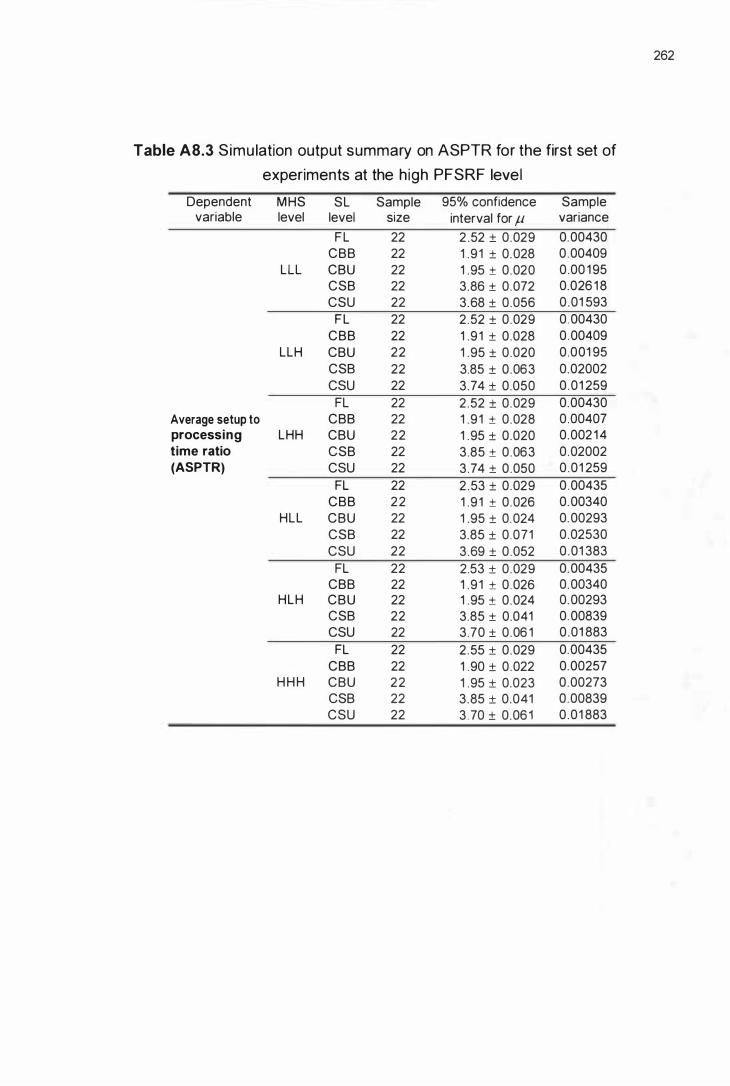
262

Table A8.3 Simu lation output summary on ASPTR for the first set of

experiments at the h igh PFSRF level

Dependent MHS SL Sample 95% confidence Sample variable level level size interval for JL variance

FL 22 2 .52 ± 0.029 0.00430 eBB 22 1 .9 1 ± 0.028 0 .00409

LLL eBU 22 1 .95 ± 0.020 0.00 1 95 eSB 22 3.86 ± 0.072 0.026 1 8 esu 22 3.68 ± 0.056 0.01 593

FL 22 2 .52 ± 0.029 0. 00430 eBB 22 1 .9 1 ± 0.028 0 .00409

LLH eBU 22 1 .95 ± 0.020 0.001 95 eSB 22 3.85 ± 0.063 0.02002 esu 22 3.74 ± 0.050 0 .01 259

FL 22 2 .52 ± 0.029 0.00430 Average setup to eBB 22 1 .9 1 ± 0.028 0.00407 processing LHH eBU 22 1 .95 ± 0.020 0.002 1 4 time ratio eSB 22 3.85 ± 0.063 0 .02002 (ASPTR) esu 22 3.74 ± 0.050 0 .01 259

FL 22 2 .53 ± 0.029 0 .00435 eBB 22 1 .9 1 ± 0.026 0.00340

HLL eBU 22 1 .95 ± 0.024 0.00293 eSB 22 3.85 ± 0 .071 0.02530 esu 22 3.69 ± 0 .052 0.01 383

FL 22 2.53 ± 0.029 0.00435 eBB 22 1 .9 1 ± 0 .026 0.00340

HLH eBU 22 1 .95 ± 0.024 0.00293 eSB 22 3.85 ± 0.041 0. 00839 esu 22 3.70 ± 0.06 1 0 .01 883

FL 22 2 .55 ± 0.029 0.00435 eBB 22 1 .90 ± 0.022 0.00257

H H H eBU 22 1 .95 ± 0.023 0.00273 eSB 22 3 .85 ± 0.041 0.00839 esu 22 3 .70 ± 0.061 0 .01 883

263

Table AS.4 Simulation output summary on AWI P for the first set of

experiments at the medium PFSRF level

Dependent MHS SL Sample 95% confidence Sample variable level level size interval for Jl variance

FL 22 63.90 ± 1 .97 1 9.69 eBB 22 62 .23 ± 1 . 56 1 2.42

LLL eBU 22 62. 1 4 ± 1 . 31 8 .76 eSB 22 1 1 1 .28 ± 8.07 3 1 5 .80 esu 22 87.20 ± 4.30 94. 1 2

FL 22 63.90 ± 1 .97 1 9.69 eBB 22 62.23 ± 1 .56 1 2 .42

LLH eBU 22 62. 1 4 ± 1 . 3 1 8 .76 eSB 22 1 1 2. 1 7 ± 8.27 347.87 esu 22 92.46 ± 5.40 1 48.06

FL 22 63.90 ± 1 . 97 1 9.69 Average work·in· eBB 22 60.67 ± 1 .68 1 4.33 process LHH eBU 22 60. 7 1 ± 1 .40 9.93 inventory eSB 22 1 1 2. 77 ± 8.27 347.87 (AWIP) esu 22 92 .46 ± 5.40 1 48.06

FL 22 63.62 ± 1 . 74 1 5.42 eBB 22 6 1 .30 ± 1 .55 1 2 . 1 7

HLL eBU 22 62 .8 1 ± 1 .38 9.72 eSB 22 1 1 1 . 53 ± 8.06 330.68 esu 22 88.98 ± 4.42 99.43

FL 22 63.62 ± 1 .74 1 5.42 eBB 22 6 1 . 30 ± 1 . 55 1 2 . 1 7

HLH eBU 22 62 .8 1 ± 1 . 38 9.72 eSB 22 1 1 6 .46 ± 9 .91 499. 1 1 esu 22 91 .89 ± 5.72 1 66 .57 FL 22 63.62 ± 1 . 74 1 5 .42

eBB 22 60.20 ± 1 .65 1 3.90 H H H eBU 22 6 1 .22 ± 1 .39 9.82

eSB 22 1 1 6.46 ± 9 .91 499. 1 1 esu 22 91 .89 ± 5.72 1 66 .57

264

Table AS.5 Simulation output summary on AFT for the first set of

experiments at the med ium PFSRF level

Dependent MHS SL Sample 95% confidence Sample variable level level size interval for f.1 variance

FL 22 8 .39 ± 0. 1 6 0. 1 254 eBB 22 8. 1 7 ± 0. 1 5 0. 1 1 45

LLL eBU 22 8. 1 9 ± 0. 1 1 0 .0564 eSB 22 1 4. 50 ± 0.95 4.43 esu 22 1 1 .46 ± 0.47 1 . 1 2

FL 22 8 .39 ± 0. 1 6 0. 1 254 eBB 22 8. 1 7 ± 0. 1 5 0. 1 1 45

LLH eBU 22 8. 1 9 ± 0. 1 1 0 .0564 eSB 22 1 4.80 ± 0.96 4 .73 esu 22 1 2 . 1 9 ± 0.62 1 .95

FL 22 8 .39 ± 0. 1 6 0. 1 254 Average flow eBB 22 7 .96 ± 0. 1 6 0. 1 296 time (AFT) LHH eBU 22 8.00 ± 0. 1 1 0 .0623

eSB 22 1 4 .80 ± 0.96 4 .73 esu 22 1 2 . 1 9 ± 0.62 1 .95

FL 22 8 .35 ± 0. 1 3 0.0858 eBB 22 8.05 ± 0. 1 5 0. 1 1 74

HLL eBU 22 8.28 ± 0 . 1 1 0 .0593 eSB 22 1 4 .57 ± 0.94 4 .51 esu 22 1 1 .70 ± 0.49 1 .23

FL 22 8 .35 ± 0. 1 3 0.0858 eBB 22 8.05 ± 0. 1 5 0. 1 1 74

HLH eBU 22 8.28 ± 0. 1 1 0 .0593 eSB 22 1 5. 1 7 ± 1 . 1 7 6.99 esu 22 1 2 . 1 0 ± 0.65 2. 1 7

FL 22 8 .35 ± 0. 1 3 0.0858 eBB 22 7.90 ± 0. 1 6 0. 1 235

HHH eBU 22 8.06 ± 0. 1 1 0 .0645 eSB 22 1 5. 1 7 ± 1 . 1 7 6.99 esu 22 1 2 . 1 0 ± 0.65 2. 1 7

265

Table A8.6 Simulation output summary on ASPTR for the first set of

experiments at the med ium PFSRF level

Dependent MHS SL Sample 95% confidence Sample variable level level size interval for JL variance

FL 22 2. 1 3 ± 0.024 0.00294 eBB 22 1 .36 ± 0.0 1 6 0 .00 1 23

LLL eBU 22 1 .38 ± 0.01 3 0.00087 eSB 22 2.65 ± 0.036 0 .00631 esu 22 2.49 ± 0.027 0.00367

FL 22 2. 1 3 ± 0.024 0.00294 eBB 22 1 .36 ± 0.0 1 6 0 .00123

LLH eBU 22 1 .38 ± 0.01 3 0.00087 eSB 22 2.63 ± 0.042 0.009 1 2 esu 22 2 .52 ± 0.027 0.00360

FL 22 2. 1 3 ± 0.024 0.00294 Average setup to eBB 22 1 .36 ± 0 .01 7 0 .00 1 44 processing LHH eBU 22 1 .38 ± 0 .01 5 0 .00 1 1 7 time ratio eSB 22 2.63 ± 0.042 0 .00912 (ASPTR) esu 22 2 .52 ± 0.027 0.00360

FL 22 2. 1 3 ± 0.020 0 .002 1 2 eBB 22 1 .35 ± 0 .01 5 0 .001 1 7

HLL eBU 22 1 .39 ± 0 .01 5 0 .00 1 2 1 eSB 22 2.65 ± 0 .031 0. 00479 esu 22 2 .48 ± 0.029 0.0041 8

FL 22 2 . 1 3 ± 0.020 0.002 1 2 eBB 22 1 . 35 ± 0.01 5 0.001 1 7

HLH eBU 22 1 . 39 ± 0 .01 5 0.00 1 2 1 eSB 22 2.66 ± 0.035 0.00633 esu 22 2 .50 ± 0 .031 0. 00475

FL 22 2. 1 3 ± 0.020 0.002 1 2 eBB 22 1 . 35 ± 0. 0 1 4 0.00096

HHH eBU 22 1 . 38 ± 0.009 0.00041 eSB 22 2.66 ± 0.035 0.00633 esu 22 2 .50 ± 0.031 0. 00475

266

Table AS.7 Simu lation output summary on AWI P for the first set of

experiments at the low PFSRF level

Dependent MHS SL Sample 95% confidence Sample variable level level size interval for J.1. variance

FL 22 96.44 ± 1 .98 1 9.96 eBB 22 7 1 .48 ± 1 .90 1 8.45

LLL eBU 22 7 1 .77 ± 2.02 20.82 eSB 22 82. 1 6 ± 4.29 93.67 esu 22 64.99 ± 2.68 36.45

FL 22 96.44 ± 1 .98 1 9.96 eBB 22 7 1 .48 ± 1 .90 1 8.45

LLH eBU 22 7 1 .77 ± 2.02 20.82 eSB 22 84.58 ± 4.48 1 02 .01 esu 22 67.64 ± 3.34 56.80

FL 22 96.44 ± 1 . 98 1 9.96 Average work·in· eBB 22 69.52 ± 1 .96 1 9.52 process LHH eBU 22 69.62 ± 2 .01 20.46 inventory eSB 22 84 .58 ± 4.48 1 02 .01 (AWIP) esu 22 67.64 ± 3.34 56.80

FL 22 94.57 ± 1 . 84 1 7.27 eBB 22 7 1 .53 ± 1 . 86 1 7.67

HLL eBU 22 72.09 ± 2. 1 5 23.55 eSB 22 82.65 ± 4.69 1 1 1 .69 esu 22 65.70 ± 3.08 48.38

FL 22 94.57 ± 1 .84 1 7 .27 eBB 22 7 1 .53 ± 1 . 86 1 7.67

HLH eBU 22 72.09 ± 2. 1 5 23.55 eSB 22 84.42 ± 4.78 1 1 6.28 esu 22 67.63 ± 3.25 53.60

FL 22 94.57 ± 1 .84 1 7.27 eBB 22 69.27 ± 1 . 75 1 5 .57

HHH eBU 22 69.48 ± 2 .06 21 .52 eSB 22 84.42 ± 4.78 1 1 6.28 esu 22 67.63 ± 3.25 53.60

267

Table AS.S Simu lation output summary on AFT for the first set of

experiments at the low PFSRF level

Dependent MHS SL Sample 95% confidence Sample variable level level size interval for J.1 variance

FL 22 8.26 ± 0. 1 2 0.074 eBB 22 6. 1 3 ± 0. 1 2 0.079

LLL eBU 22 6. 1 5 ± 0. 1 1 0 .065 eSB 22 7 .04 ± 0.33 0 .563 esu 22 5 .57 ± 0. 1 8 0. 1 58

FL 22 8.26 ± 0. 1 2 0.074 eBB 22 6. 1 3 ± 0. 1 2 0.079

LLH eBU 22 6. 1 5 ± 0. 1 1 0.065 eSB 22 7.24 ± 0.35 0.632 esu 22 5 .79 ± 0.23 0.27 1

FL 22 8.26 ± 0 . 1 2 0.074 Average flow eBB 22 5 .96 ± 0. 1 3 0.089 time (AFT) LHH eBU 22 5 .96 ± 0. 1 2 0.069

eSB 22 7 .24 ± 0.35 0.632 esu 22 5 .79 ± 0.23 0.271

FL 22 8. 1 0 ± 0. 1 1 0.06 1 eBB 22 6. 1 4 ± 0. 1 2 0.077

HLL eBU 22 6. 1 7 ± 0. 1 2 0.079 eSB 22 7.08 ± 0 .36 0.659 esu 22 5.63 ± 0 .21 0.225

FL 22 8. 1 0 ± 0 . 1 1 0.061 eBB 22 6. 1 4 ± 0. 1 2 0.077

HLH eBU 22 6. 1 7 ± 0. 1 2 0.079 eSB 22 7.23 ± 0 .37 0 .702 esu 22 5.79 ± 0.22 0.257

FL 22 8. 1 0 ± 0. 1 1 0.061 eBB 22 5 .94 ± 0. 1 1 0 .065

HHH eBU 22 5.95 ± 0. 1 2 0.07 1 eSB 22 7.23 ± 0 .37 0 .702 esu 22 5.79 ± 0.22 0.257

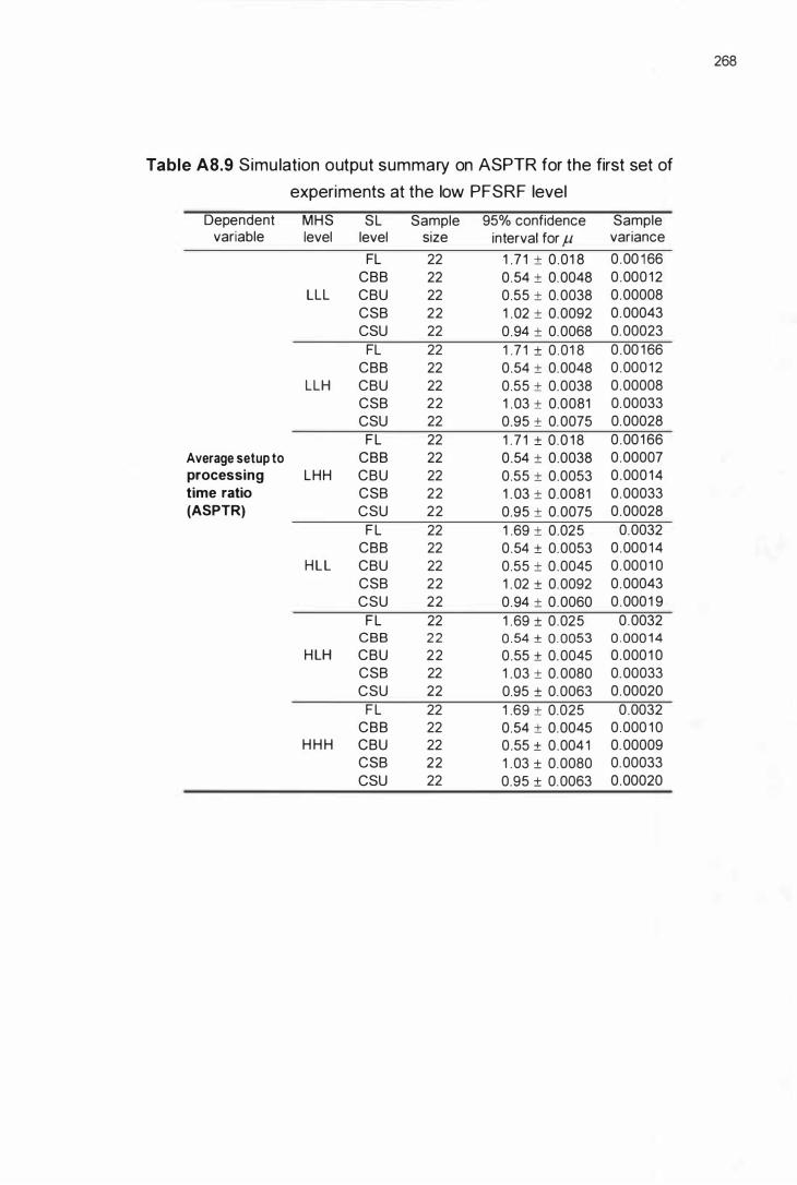
268

Table A8.9 Simu lation output summary on ASPTR for the first set of

experiments at the low PFSRF level

Dependent MHS SL Sample 95% confidence Sample variable level level size interval for f.1 variance

FL 22 1 .7 1 ± 0 .01 8 0 .00 1 66 eBB 22 0 .54 ± 0.0048 0 .00012

LLL eBU 22 0.55 ± 0. 0038 0.00008 eSB 22 1 .02 ± 0.0092 0.00043 esu 22 0.94 ± 0.0068 0.00023

FL 22 1 .7 1 ± 0.01 8 0 .00 1 66 eBB 22 0 .54 ± 0.0048 0 .00012

LLH eBU 22 0.55 ± 0.0038 0.00008 eSB 22 1 .03 ± 0.0081 0.00033 esu 22 0.95 ± 0. 0075 0.00028 FL 22 1 . 7 1 ± 0.0 1 8 0 .001 66

Average setup to eBB 22 0 .54 ± 0.0038 0.00007 processing LHH eBU 22 0.55 ± 0.0053 0 .00014 time ratio eSB 22 1 . 03 ± 0.0081 0.00033 (ASPTR) esu 22 0.95 ± 0.0075 0.00028

FL 22 1 .69 ± 0.025 0.0032 eBB 22 0 .54 ± 0.0053 0 .00014

HLL eBU 22 0.55 ± 0.0045 0 .0001 0 eSB 22 1 . 02 ± 0.0092 0.00043 esu 22 0.94 ± 0.0060 0 .0001 9

FL 22 1 .69 ± 0.025 0.0032 eBB 22 0 . 54 ± 0. 0053 0 . 000 1 4

HLH eBU 22 0 .55 ± 0.0045 0.0001 0 eSB 22 1 .03 ± 0.0080 0.00033 esu 22 0.95 ± 0.0063 0.00020

FL 22 1 .69 ± 0.025 0.0032 eBB 22 0.54 ± 0.0045 0.000 1 0

H H H eBU 22 0 .55 ± 0.004 1 0.00009 eSB 22 1 .03 ± 0.0080 0.00033 esu 22 0.95 ± 0.0063 0.00020

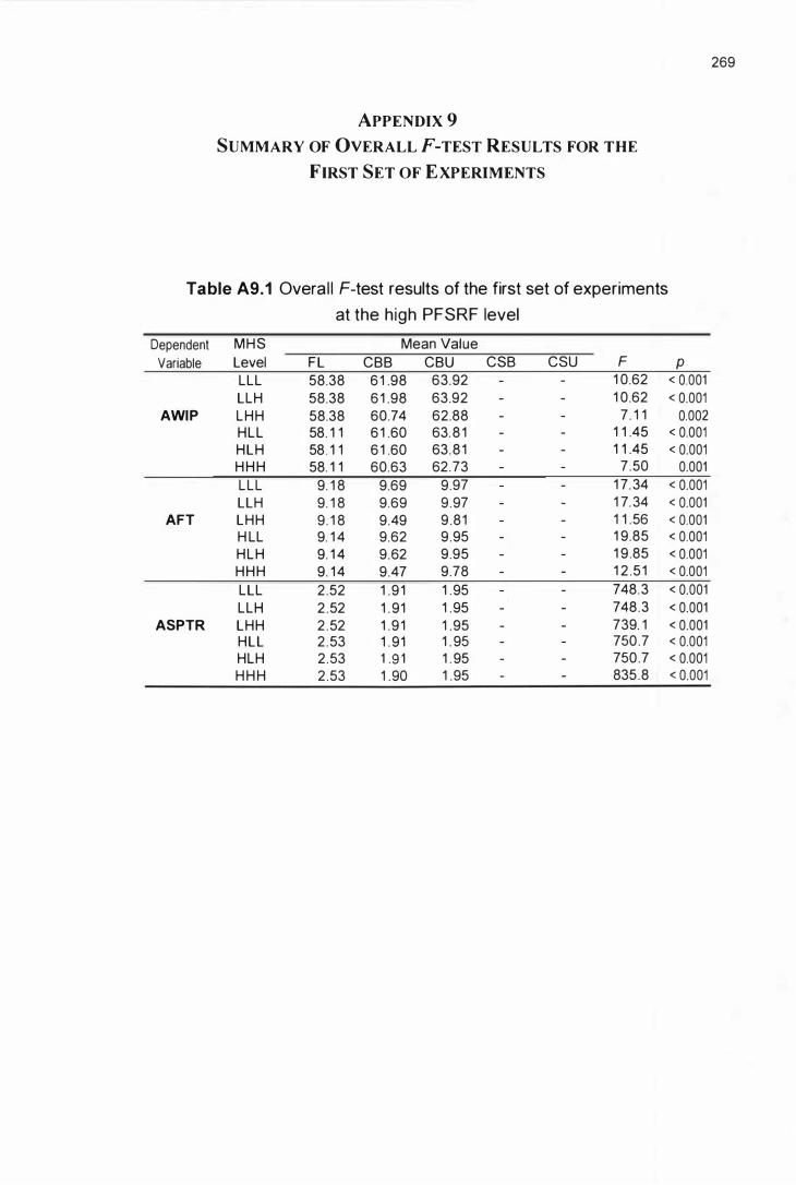
ApPENDIX 9 SUMMARY OF OVERALL F-TEST RESULTS FOR THE

FIRST SET OF E XPERIMENTS

Ta ble A9.1 Overal l F-test results of the first set of experiments

at the h igh PFSRF level

Dependent MHS Mean Value Variable Level FL eBB eBU eSB esu F

LLL 58.38 6 1 .98 63.92 1 0.62 LLH 58.38 6 1 .98 63.92 1 0.62

AWIP LHH 58.38 60.74 62.88 7 . 1 1 HLL 58. 1 1 6 1 .60 63. 8 1 1 1 .45 HLH 58 . 1 1 6 1 .60 63.8 1 1 1 .45 H H H 58. 1 1 60.63 62.73 7 .50 LLL 9. 1 8 9.69 9.97 1 7. 34 LLH 9. 1 8 9.69 9.97 1 7. 34

AFT LHH 9. 1 8 9.49 9 .81 1 1 .56 H LL 9. 1 4 9.62 9.95 1 9.85 HLH 9. 1 4 9.62 9.95 1 9 .85 HHH 9. 1 4 9.47 9.78 1 2 .5 1 LLL 2 .52 1 .9 1 1 .95 748.3 LLH 2 .52 1 . 91 1 .95 748.3

ASPTR LHH 2 .52 1 .9 1 1 .95 739. 1 HLL 2 .53 1 . 91 1 . 95 750.7 HLH 2 .53 1 .9 1 1 . 95 750.7 H H H 2.53 1 .90 1 .95 835.8

269

p < 0.001 < 0.001

0.002 < 0.001 < 0.001

0.001 < 0.001 < 0.001 < 0.001 < 0.001 < 0.001 < 0.001 < 0.001 < 0.001 < 0.001 < 0.001 < 0.001 < 0.001

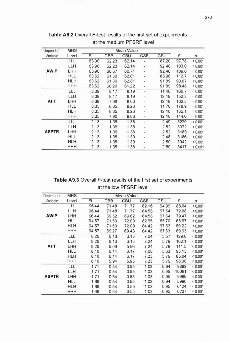
270

Table A9.2 Overa l l F-test results of the first set of experiments

at the medium PFSRF level

Dependent MHS Mean Value Variable Level FL eBB eBU eSB esu F p

LLL 63.90 62.23 62. 1 4 87.20 97.78 < 0.001 LLH 63.90 62.23 62. 1 4 92 .46 1 03 .0 < 0.001

AWIP LHH 63.90 60.67 60. 7 1 92.46 1 09.0 < 0.001 H LL 63.62 6 1 .30 62.8 1 88.98 1 1 2 .7 < 0.001 HLH 63.62 6 1 .30 62. 81 91 .89 93.07 < 0.001 H H H 63.62 60.20 6 1 .22 91 .89 98.48 < 0.001 LLL 8 .39 8. 1 7 8. 1 9 1 1 .46 1 60 .7 < 0.001 LLH 8 .39 8. 1 7 8. 1 9 1 2 . 1 9 1 52 .3 < 0.001

AFT LHH 8 .39 7.96 8.00 12 . 1 9 1 62.3 < 0.001 H LL 8 .35 8.05 8.28 1 1 . 70 1 78.9 < 0.001 HLH 8.35 8.05 8.28 1 2 . 1 0 1 36 . 1 < 0.001 H H H 8.35 7.90 8.06 1 2 . 1 0 1 44.6 < 0.001 LLL 2. 1 3 1 . 36 1 .38 2.49 3220 < 0.001 LLH 2. 1 3 1 . 36 1 .38 2 .52 3372 < 0.001

ASPTR LHH 2. 1 3 1 . 36 1 . 38 2 .52 3 1 89 < 0.001 HLL 2. 1 3 1 . 35 1 .39 2.48 3 1 86 < 0.001 HLH 2. 1 3 1 . 35 1 .39 2 .50 3042 < 0.001 H H H 2. 1 3 1 . 35 1 .38 2 .50 34 1 7 < 0.001

Table A9.3 Overal l F-test resu lts of the fi rst set of experiments

at the low PFSRF level

Dependent MHS Mean Value Variable Level FL eBB eBU eSB esu F p

LLL 96.44 7 1 .48 7 1 . 77 82. 1 6 64.99 88.04 < 0.001 LLH 96.44 7 1 .48 7 1 . 77 84.58 67.64 72.08 < 0.001

AWIP LHH 96.44 69.52 69.62 84.58 67.64 79.47 < 0.001 HLL 94.57 7 1 . 53 72.09 82.65 65.70 65.67 < 0.001 HLH 94.57 7 1 .53 72.09 84 .42 67.63 60.22 < 0.001 HHH 94. 57 69.27 69.48 84.42 67.63 69.63 < 0.001 LLL 8.26 6. 1 3 6. 1 5 7 .04 5.57 1 29.6 < 0.001 LLH 8.26 6. 1 3 6. 1 5 7 .24 5.79 1 02. 1 < 0.001

AFT LHH 8.26 5.96 5 .96 7. 24 5.79 1 1 1 . 5 < 0.001 H LL 8. 1 0 6 . 1 4 6 . 1 7 7 .08 5.63 95. 1 3 < 0.001 HLH 8. 1 0 6 . 1 4 6. 1 7 7.23 5.79 85.04 < 0.001 H H H 8. 1 0 5 .94 5.95 7.23 5.79 98.30 < 0.001 LLL 1 . 7 1 0.54 0.55 1 .02 0.94 9882 < 0.001 LLH 1 . 7 1 0.54 0.55 1 .03 0.95 1 0081 < 0.001

ASPTR LHH 1 . 7 1 0.54 0.55 1 .03 0.95 9999 < 0.001 H LL 1 .69 0.54 0.55 1 .02 0.94 5990 < 0.001 HLH 1 .69 0.54 0 .55 1 . 03 0.95 6 1 24 < 0.001 H H H 1 .69 0.54 0 .55 1 .03 0.95 6237 < 0.001

APPENDIX 1 0

RESULTS OF PLANNED COMPARISONS FOR THE

FIRST SET OF EXPERIMENTS

Table A1 0.1 Resu lts of planned comparisons for AWI P

at the high PFSRF level

Dependent MHS Hypotheses Variable Level Tested dr F p

LLL Ho( 1 a) 42 2 .04 0. 1 6 Ho(3) 59 24.76 < 0.00 1

LLH Ho( 1 a) 42 2 .04 0. 1 6 Ho(3) 59 24.76 < 0.00 1

L H H Ho( 1 a) 4 1 2 .61 0. 1 1 AWIP Ho(3) 58 14 .34 < 0.001

HLL Ho( 1 a) 4 1 2 .81 0. 1 0 Ho(3) 56 24.55 < 0.001

HLH Ho( 1 a) 41 2 .81 0 . 1 0 Ho(3) 56 24.55 < 0.001

HHH Ho( 1 a) 42 2 .56 0. 1 2 Ho(3) 56 1 4.92 < 0.001

* df - degrees of freedom

Table A 1 0.2 Resu lts of planned comparisons for AFT

at the high PFSRF level

Dependent MHS Hypotheses Variable Level Tested df F P

LLL Ho( 1 a) 4 1 3.42 0.072 Ho(3) 62 42.72 < 0.001

LLH Ho( 1 a) 4 1 3.42 0 .072 Ho(3) 62 42.72 < 0.001

LHH Ho( 1 a) 38 4 .72 0.036 AFT Ho(3) 58 23.65 < 0.001

HLL Ho( 1 a) 38 4.99 0.032

Ho(3) 58 46. 1 5 < 0.001

HLH Ho( 1 a) 38 4.99 0.032 Ho(3) 58 46. 1 5 < 0.001

HHH Ho( 1 a) 41 4.66 0.037 Ho(3) 6 1 26.32 < 0.001

271

272

Table A1 0.3 Resu lts of planned comparisons for ASPTR

at the hig h PFSRF level

Dependent MHS Hypotheses Variable Level Tested df F P

LLL Ho( 1 a) 37 3.79 0.059 Ho(3) 36 1 328 < 0.001

LLH Ho( 1 a) 37 3.79 0.059 Ho(3) 36 1 328 < 0.001

LHH Ho( 1 a) 38 6 .89 0 .01 2 ASPTR Ho(3) 36 1 321 < 0.001

HLL Ho( 1 a) 42 6 .35 0.0 1 6 Ho(3) 37 1 346 < 0.001

H LH Ho( 1 a) 42 6 .35 0.0 1 6 Ho(3) 37 1 346 < 0.001

H H H Ho( 1 a) 42 7. 1 0 0 .01 1 Ho(3) 34 1 4 1 6 < 0.001

Table A 1 0.4 Resu lts of planned comparisons for AWI P

at the medium PFSRF level

Dependent MHS Hypotheses Variable Level Tested df F P

Ho( 1 a) 4 1 0 .0078 n .s . LLL Ho(2) 23 1 38.4 < 0.001

Ho(3) 33 2 .59 0. 1 2

Ho( 1 a) 41 0 .0078 n .s . LLH Ho(2) 23 1 3 1 .4 < 0.001

Ho(3) 33 2 .59 0. 1 2

Ho( 1 a) 41 0 .00 1 1 n .s. LHH Ho(2) 23 1 44. 1 < 0.001

AWIP Ho(3) 34 8.82 0.005

Ho( 1 a) 41 2 .29 0. 1 4 H L L Ho(2) 23 1 51 .9 < 0.001

Ho(3) 36 2 .57 0. 1 2

Ho( 1 a) 41 2.29 0. 1 4 HLH Ho(2) 22 1 1 3.8 < 0.001

Ho(3) 36 2 .57 0. 1 2

Ho( 1 a) 41 0.97 n .s. H H H Ho(2) 23 1 24 .0 < 0.001

Ho(3) 37 8 .76 0.005

*n . s. = not statistically significant

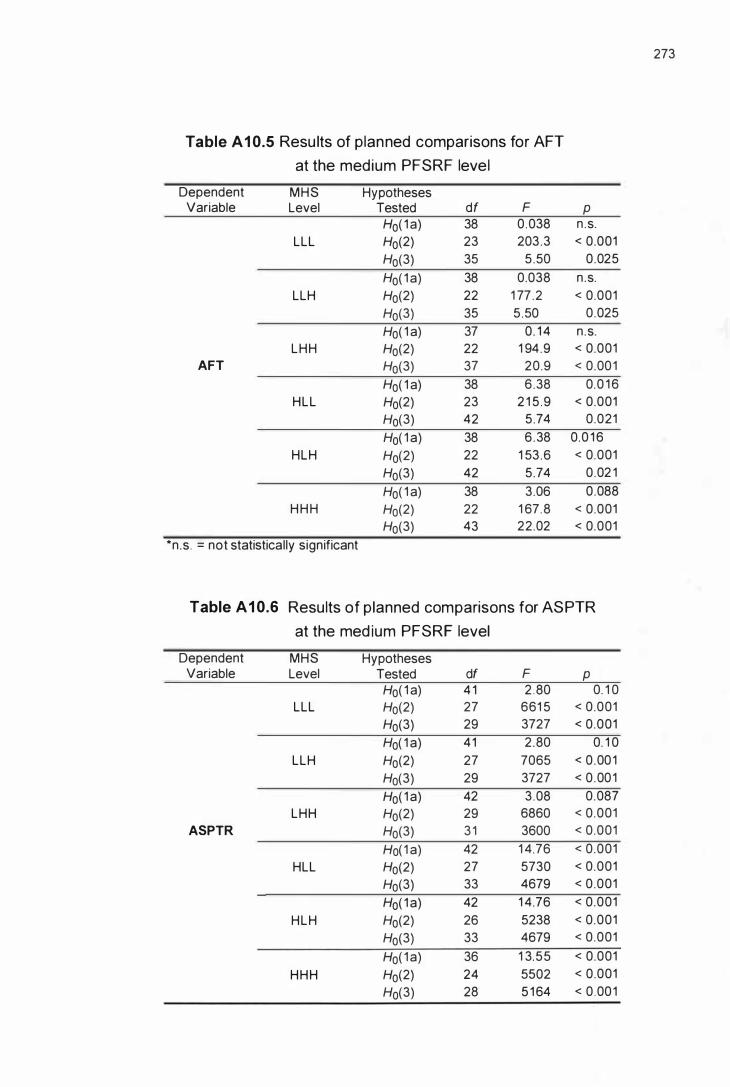
273

Table A 1 0.5 Resu lts of planned comparisons for AFT

at the medium PFSRF level

Dependent MHS Hypotheses Variable Level Tested df F P

Ho( 1 a) 38 0.038 n .s. LLL Ho(2) 23 203 .3 < 0.001

Ho(3) 35 5 .50 0.025

Ho( 1 a) 38 0.038 n .s. LLH Ho(2) 22 1 77 .2 < 0.001

Ho(3) 35 5 .50 0.025

Ho( 1 a) 37 0. 1 4 n .s. LHH Ho(2) 22 1 94 .9 < 0.001

AFT Ho(3) 37 20.9 < 0.001

Ho( 1 a) 38 6 .38 0.0 1 6 HLL Ho(2) 23 2 1 5 .9 < 0.001

Ho(3) 42 5.74 0.021

Ho( 1 a) 38 6 .38 0.0 1 6 HLH Ho(2) 22 1 53 .6 < 0.001

Ho(3) 42 5.74 0.02 1

Ho( 1 a) 38 3.06 0.088 H H H Ho(2) 22 1 67.8 < 0.001

Ho(3) 43 22.02 < 0.001

*n.s . - not statistically significant

Table A 1 0.6 Results of planned comparisons for ASPTR

at the med ium PFSRF level

Dependent MHS Hypotheses Variable Level Tested df F P

Ho( 1 a) 4 1 2 .80 0. 1 0 LLL Ho(2) 27 661 5 < 0.001

Ho(3) 29 3727 < 0.001

Ho( 1 a) 41 2.80 0. 1 0 LLH Ho(2) 27 7065 < 0.001

Ho(3) 29 3727 < 0.001

Ho( 1 a) 42 3 .08 0.087 LHH Ho(2) 29 6860 < 0.001

ASPTR Ho(3) 3 1 3600 < 0.001

Ho( 1 a) 42 1 4.76 < 0.001

HLL Ho(2) 27 5730 < 0.001 Ho(3) 33 4679 < 0.001

Ho( 1 a) 42 1 4.76 < 0.001

HLH Ho(2) 26 5238 < 0.001 Ho(3) 33 4679 < 0.001

Ho( 1 a) 36 1 3.55 < 0.001

HHH Ho(2) 24 5502 < 0.001

Ho(3) 28 5 1 64 < 0 .001

274

Table A1 0.7 Resu lts of planned comparisons for AWI P

at the low PFSRF level

Dependent MHS Hypotheses Variable Level Tested df F P

Ho( 1 a) 42 0 .049 n.s. LLL Ho( 1 b) 35 49.88 < 0.001

Ho(2) 55 1 . 97 0. 1 7 Ho(3) 44 409 .4 < 0.001

Ho( 1 a) 42 0.05 n .s. LLH Ho( 1 b) 39 39.78 < 0.00 1

Ho(2) 57 8 .93 0.004 Ho(3) 42 455 .0 < 0.001

Ho( 1 a) 42 0 .005 n .s . LHH Ho( 1 b) 39 39.78 < 0.001

Ho(2) 58 1 8.94 < 0.001 AWIP Ho(3) 42 530.4 < 0.001

Ho( 1 a) 4 1 0. 1 7 n .s . HLL Ho( 1 b) 36 39.52 < 0.001

Ho(2) 54 2.45 0. 1 2 Ho(3) 52 343. 1 < 0.001

Ho( 1 a) 4 1 0. 1 7 n .s . HLH Ho( 1 b) 37 36. 5 1 < 0.001

Ho(2) 54 7.40 0.009 Ho(3) 45 4 1 3.2 < 0.001

Ho( 1 a) 4 1 0 .028 n .s . HHH Ho( 1 b) 37 36.5 1 < 0. 001

Ho(2) 53 1 8. 79 < 0.001 Ho(3) 43 526 .0 < 0.001

*n.s. = not statistically significant

275

Table A1 0.8 Resu lts of planned comparisons for AFT

at the low PFSRF level

Dependent MHS Hypotheses Variable Level Tested df F P

Ho( 1 a) 42 0.046 n .s. LLL Ho( 1 b) 32 66.28 < 0.001

Ho(2) 45 2 .77 0. 1 0 Ho(3) 50 709.4 < 0.001

Ho( 1 a) 42 0.046 n .s. LLH Ho( 1 b) 36 50.97 < 0.001

Ho(2) 48 1 2. 08 0.001 Ho(3) 4 1 894 .8 < 0.001

Ho( 1 a) 41 0.0003 n .s. LHH Ho( 1 b) 36 50.97 < 0.001

Ho(2) 49 25.53 < 0.001 AFT Ho(3) 43 1 0 1 7 < 0.001

Ho( 1 a) 42 0.20 n .s. HLL Ho( 1 b) 34 52 .5 1 < 0.001

Ho(2) 46 3.25 0 .078 Ho(3) 59 591 . 9 < 0.001

Ho( 1 a) 42 0.20 n .s. HLH Ho( 1 b) 35 47.04 < 0.001

Ho(2) 46 9 .96 0.003 Ho(3) 47 826.6 < 0.001 Ho( 1 a) 42 0.0 1 2 n .s.

H H H Ho( 1 b) 35 47.04 < 0.001 Ho(2) 44 25.59 < 0.001 Ho(3) 44 1 067 < 0.001

*n.s . - not statistically significant

276

Table A 1 0.9 Resu lts of planned comparisons for ASPTR

at the low PFSRF level

Dependent MHS Hypotheses Variable Level Tested df F P

Ho( 1 a) 40 1 0. 32 0.003 LLL Ho( 1 b) 39 229 .8 < 0.001

Ho(2) 60 1 9275 < 0.001 Ho(3) 22 1 7340 < 0.001

Ho( 1 a) 40 1 0. 32 0.003 LLH Ho( 1 b) 42 255. 1 < 0.001

Ho(2) 65 21 344 < 0.001 Ho(3) 22 1 7340 < 0.001

Ho( 1 a) 38 1 4 .25 < 0.001 LHH Ho( 1 b) 42 255. 1 < 0.001

Ho(2) 67 208 1 6 < 0.001 ASPTR Ho(3) 22 1 7292 < 0.001

Ho( 1 a) 41 1 0.76 0.002 HLL Ho( 1 b) 36 240. 1 < 0.001

Ho(2) 62 1 9226 < 0.001 Ho(3) 22 8892 < 0.001

Ho( 1 a) 4 1 1 0 . 76 0.002 HLH Ho(1 b) 40 243 .3 < 0.001

Ho(2) 70 22090 < 0.001

Ho(3) 22 8892 < 0.001

Ho( 1 a) 42 1 7 .46 < 0.001 H H H Ho( 1 b) 40 243 .3 < 0.001

Ho(2) 65 23992 < 0.001 Ho(3) 22 8968 < 0.001

APPENDIX 1 1

DEPENDENT VARIABLE MOVING AVERAGE PLOTS FOR

THE SECOND SET OF EXPERIMENTS

250

VI 200 t t<3 ..e- 1 50

o ....

� 1 00 E ::s Z 50

o

Period ( 1 20 hrs)

Figure A 1 1 . 1 Moving average plot for average work-in-process inventory

(Cel lu lar layout with SUPC and backtracking flow al lowed)

VI .... ::s 0

..c

35 .0

30.0

25.0

20.0

1 5 .0

1 0.0

5.0

0.0 - c- M '" V") - - N

Period ( 1 20 hrs)

Figure A 1 1 .2 Moving average plot for average flow time

(Cel lu lar layout with SUPC and backtracking flow al lowed)

277

'$.

50.0

40.0

30.0

20.0

1 0.0

0.0

Period ( 1 20 h rs)

Figure A 1 1 .3 Moving average plot for average machine uti l isation

(Cel lu lar layout with SUPC and backtracking flow al lowed)

278

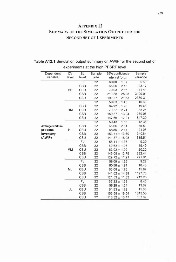
APPENDIX 1 2

SUMMARY OF THE SIMULATION OUTPUT FOR THE

SECOND SET OF E XPERIMENTS

Table A 1 2. 1 Simulation output summary on AWI P for the second set of

experiments at the h igh PFSRF level

Dependent CV SL Sample 95% confidence Sample variable level level size interval for J.1 variance

FL 22 60.08 ± 1 . 37 9.60 eBB 22 65.06 ± 2. 1 3 23. 1 7

HH eBU 22 70.03 ± 2.85 41 .4 1 eSB 22 21 9 .88 ± 25.08 3 1 99 .01 esu 22 1 99.27 ± 21 .63 2380 .31

FL 22 59.63 ± 1 .45 1 0.63 eBB 22 64.92 ± 1 .96 1 9.45

H M eBU 22 70 .33 ± 2.74 38.25 eSB 22 1 59.37 ± 1 3.94 989.08 esu 22 1 47 .66 ± 1 2 .9 1 847 .39

FL 22 59.43 ± 1 .56 12 .36 Average work·in· eBB 22 65.66 ± 2.64 35. 5 1 process HL eBU 22 68.86 ± 2. 1 7 24.05 inventory eSB 22 1 53. 1 1 ± 1 3 .60 940.64 (AWIP) esu 22 1 4 1 . 37 ± 1 6.08 1 31 5.5 1

FL 22 58. 1 1 ± 1 .36 9 .39 eBB 22 60.63 ± 1 .96 1 9.49

MM eBU 22 63.92 ± 1 .99 20.20 eSB 22 1 45.09 ± 1 2 .79 832.44 esu 22 1 29 .72 ± 1 1 . 9 1 721 .6 1

FL 22 58.09 ± 1 .35 9.22 eBB 22 60.56 ± 1 . 9 1 1 8.46

ML eBU 22 63.08 ± 1 .76 1 5.82 eSB 22 1 4 1 .62 ± 1 4.89 1 1 27 .75 esu 22 1 2 1 . 53 ± 1 1 .83 7 1 2 .20

FL 22 57.22 ± 1 .29 8.45 eBB 22 58.28 ± 1 .64 1 3.67

LL eBU 22 6 1 .53 ± 1 . 72 1 5.08 eSB 22 1 53 .59 ± 1 9 .04 1 843.50 esu 22 1 1 3. 32 ± 1 0 .47 557.69

279

280

Table A 1 2.2 Simulation output summary on AFT for the second set of

experiments at the h igh PFSRF level

Dependent ev SL Sample 95% confidence Sample variable level level size interval for J.1 variance

FL 22 9 .46 ± 0. 1 7 0. 1 468 eBB 22 1 0. 1 7 ± 0.25 0 .31 99

HH eBU 22 1 0.90 ± 0.32 0 .51 04 eSB 22 34.72 ± 3.74 7 1 .34 esu 22 3 1 .06 ± 3. 1 6 50.66

FL 22 9 .38 ± 0. 1 4 0. 0994 eBB 22 1 0. 1 5 ± 0.23 0.2683

HM CBU 22 1 0.96 ± 0.30 0.4721 eSB 22 24.97 ± 2.00 20.42 esu 22 23.05 ± 1 .89 1 8. 1 3 FL 22 9 .35 ± 0. 1 6 0. 1 285

Average flow eBB 22 1 0.26 ± 0.33 0. 5394 time (AFT) H L eBU 22 1 0.73 ± 0.25 0. 3 1 83

eSB 22 23.91 ± 2.00 20.36 esu 22 22.03 ± 2 .21 24.92

FL 22 9 . 1 4 ± 0. 1 3 0.08 1 7 eBB 22 9.47 ± 0.23 0.2602

MM eBU 22 9.97 ± 0.21 0.2305 eSB 22 22.92 ± 1 .98 1 9.94 esu 22 20.37 ± 1 .70 1 4.64

FL 22 9. 1 4 ± 0. 1 3 0.0868 eBB 22 9.46 ± 0.22 0.2479

ML eBU 22 9 .95 ± 0. 1 9 0. 1 853 eSB 22 22.30 ± 2 .31 27.05 esu 22 1 8.96 ± 1 .68 1 4.44

FL 22 9 .01 ± 0. 1 2 0.0789 eBB 22 9. 1 1 ± 0. 1 9 0. 1 826

LL eBU 22 9 .60 ± 0. 1 9 0. 1 863 eSB 22 24.38 ± 3.08 48.23 esu 22 1 7.75 ± 1 .46 1 0.84

281

Table A 1 2.3 Simu lation output summary on ASPTR for the second set of

experiments at the high PFSRF level

Dependent CV SL Sample 95% confidence Sample variable level level size interval for f.1 variance

FL 22 2 .52 ± 0.03 0.00593 eBB 22 1 .9 1 ± 0 .03 0.00331

HH eBU 22 1 .97 ± 0 .03 0.00439 eSB 22 3.95 ± 0.06 0.0 1 81 7 esu 22 3 .94 ± 0.08 0.02987

FL 22 2 .50 ± 0.03 0.00559 eBB 22 1 .93 ± 0.03 0.00333

HM eBU 22 1 .96 ± 0.02 0.00299 eSB 22 3 .79 ± 0.06 0 .01 9 1 8 esu 22 3.68 ± 0.04 0.00808

FL 22 2 .51 ± 0.03 0. 00457 Average setup to eBB 22 1 .9 1 ± 0.03 0.00377 processing H L eBU 22 1 .95 ± 0.02 0.001 90 time ratio eSB 22 3.74 ± 0.06 0 .020 1 2 (ASPTR) esu 22 3.68 ± 0.06 0 .02 1 05

FL 22 2.53 ± 0.03 0.00435 eBB 22 1 .90 ± 0.02 0.00257

MM eBU 22 1 .95 ± 0.02 0 .00 1 95 eSB 22 3 .85 ± 0.04 0.00839 esu 22 3 .70 ± 0.06 0 .01 883 FL 22 2 .54 ± 0.03 0.00506

eBB 22 1 .9 1 ± 0.02 0 .002 1 9 M L eBU 22 1 .94 ± 0.02 0.00280

eSB 22 3.82 ± 0.07 0.02 1 60 esu 22 3.69 ± 0.07 0.02234

FL 22 2.55 ± 0.02 0.00293 eBB 22 1 .9 1 ± 0.02 0.00278

LL eBU 22 1 .94 ± 0.03 0.00393 eSB 22 3 .91 ± 0.06 0 .01 759 esu 22 3 .67 ± 0.05 0 .01 207

282

Table A 1 2.4 Simu lation output summary on AWI P for the second set of

experiments at the medium PFSRF level

Dependent CV SL Sample 95% confidence Sample variable level level size interval for J.1. variance

FL 22 65. 5 1 ± 1 .92 1 8. 7 1 eBB 22 65.04 ± 1 . 70 1 4.66

HH eBU 22 64.57 ± 1 .68 1 4. 36 eSB 22 1 55.62 ± 1 2 .35 775.68 esu 22 1 29.57 ± 1 0.22 530.95

FL 22 65.55 ± 2.05 21 .43 eBB 22 64.93 ± 2 .01 20.54

HM eBU 22 64.27 ± 1 .57 12 .56 eSB 22 1 1 9.06 ± 9. 1 4 424.99 esu 22 99.94 ± 5.80 1 70. 89

FL 22 65.54 ± 2 .01 20.64 Average work·in· eBB 22 65. 1 4 ± 1 . 98 1 9.92 process H L eBU 22 63.93 ± 1 .46 1 0.86 inventory eSB 22 1 1 3.21 ± 6.08 1 88 .32 (AWIP) esu 22 95.73 ± 5.36 1 46.04

FL 22 63.62 ± 1 . 74 1 5.42 eBB 22 6 1 .30 ± 1 . 55 1 2 . 1 7

MM eBU 22 60.7 1 ± 1 .40 9.93 eSB 22 1 1 6 .46 ± 9 .91 499. 1 1 esu 22 91 .89 ± 5.72 1 66 .57

FL 22 63.82 ± 1 . 8 1 1 6.73 eBB 22 6 1 .47 ± 1 .6 1 1 3. 1 3

ML eBU 22 60.62 ± 1 .30 8 .54 eSB 22 1 08 .31 ± 7 .06 253.64 esu 22 88. 5 1 ± 4 .73 1 14 .03 FL 22 62 .59 ± 1 .70 1 4.70

eBB 22 60. 1 7 ± 1 .39 9.85 LL eBU 22 59.22 ± 1 . 30 8.62

eSB 22 1 1 2.83 ± 9.85 493.84 esu 22 82 .57 ± 3.29 55.2 1

283

Table A 1 2.5 Simu lation output summary on AFT for the second set of

experiments at the med ium PFSRF level

Dependent CV SL Sample 95% confidence Sample variable level level size interval for j.l variance

FL 22 8.60 ± 0. 1 6 0. 1 363 eBB 22 8 .54 ± 0. 1 6 0. 1 301

HH eBU 22 8.50 ± 0. 1 5 0. 1 1 6 1 eSB 22 20.38 ± 1 .49 1 1 .26 esu 22 1 7 .04 ± 1 .24 7.76

FL 22 8.60 ± 0. 1 7 0. 1 5 1 5 eBB 22 8 .52 ± 0.20 0.2072

HM eBU 22 8.47 ± 0. 1 3 0.0883 eSB 22 1 5.56 ± 1 .07 5.85 esu 22 1 3 . 1 4 ± 0.65 2. 1 5

FL 22 8.60 ± 0. 1 7 0 . 1 437 Average flow eBB 22 8 .55 ± 0.20 0.20 1 3 time (AFT) HL eBU 22 8.43 ± 0. 1 3 0.087 1

eSB 22 1 4.87 ± 0 .70 2.47 esu 22 1 2 .60 ± 0.60 1 .83

FL 22 8 .35 ± 0. 1 3 0.0858 eBB 22 8.05 ± 0. 1 5 0. 1 1 74

MM eBU 22 8.00 ± 0. 1 1 0 .0623 eSB 22 1 5 . 1 7 ± 1 . 1 7 6.99 esu 22 1 2 . 1 0 ± 0.65 2. 1 7

FL 22 8 .38 ± 0 . 1 4 0. 1 053 eBB 22 8.07 ± 0. 1 5 0. 1 1 90

ML eBU 22 7.99 ± 0 . 1 0 0.0495 eSB 22 14 . 1 1 ± 0.82 3.43 esu 22 1 1 .64 ± 0 .52 1 .36

FL 22 8 .2 1 ± 0. 1 4 0.0956 eBB 22 7.90 ± 0. 1 2 0.0728

LL eBU 22 7.80 ± 0. 1 0 0.05 1 8 eSB 22 1 4 .74 ± 1 . 1 8 7 .07 esu 22 1 0 .88 ± 0 .33 0.56

284

Table A 1 2.6 Simulation output summary on ASPTR for the second set of

experiments at the medium PFSRF level

Dependent CV SL Sample 95% confidence Sample variable level level size interval for f.1 variance

FL 22 2 . 1 2 ± 0.03 0.00346 eBB 22 1 .37 ± 0 .01 0. 00082

HH eBU 22 1 .38 ± 0 .01 0 .00 1 1 2 eSB 22 2.77 ± 0.04 0.00727 esu 22 2.66 ± 0.03 0.00533

FL 22 2 . 1 2 ± 0.04 0.00645 eBB 22 1 .36 ± 0.02 0.001 42

HM eBU 22 1 .38 ± 0 .01 0 .001 00 eSB 22 2 .59 ± 0.04 0.00651 esu 22 2.49 ± 0.04 0.00655

FL 22 2 . 1 4 ± 0.03 0.00335 Average setup to eBB 22 1 .35 ± 0 .01 0.00 1 07 processing H L eBU 22 1 .37 ± 0 .01 0 .00081 time ratio eSB 22 2 .58 ± 0.04 0.00745 (ASPTR) esu 22 2.49 ± 0.03 0.00565

FL 22 2. 1 3 ± 0.02 0 .002 1 2 eBB 22 1 .35 ± 0.02 0.001 1 7

MM eBU 22 1 .38 ± 0.02 0.001 1 7 eSB 22 2 .66 ± 0.04 0.00633 esu 22 2 .50 ± 0.03 0.00475

FL 22 2. 1 5 ± 0.03 0.00322 eBB 22 1 .35 ± 0.02 0.001 1 7

M L eBU 22 1 .37 ± 0 .01 0 .00091 eSB 22 2.63 ± 0.04 0.00860 esu 22 2.50 ± 0.02 0.00277

FL 22 2. 1 4 ± 0.03 0.00393 eBB 22 1 .36 ± 0.01 0 .00 1 08

LL eBU 22 1 . 37 ± 0.01 0 .00 1 1 3 eSB 22 2.68 ± 0.03 0.00569 esu 22 2.48 ± 0.02 0.00262

285

Table A 1 2.7 Simu lation output summary on AWI P for the second set of

experiments at the low PFSRF level

Dependent CV SL Sample 95% confidence Sample variable level level size interval for J..l variance

FL 22 98.88 ± 2 .56 33.43 eBB 22 7 1 .04 ± 1 .77 1 5.86

H H eBU 22 7 1 .44 ± 2 .31 27.07 eSB 22 92.40 ± 6 .66 225.82 CSU 22 74.93 ± 3 .81 73.86

FL 22 99.35 ± 2.84 4 1 . 1 1 eBB 22 70.75 ± 1 .93 1 9.03

HM eBU 22 70.85 ± 2.23 25.35 eSB 22 83.48 ± 4.49 1 02 .75 esu 22 69.27 ± 2 .89 42.49

FL 22 99. 1 1 ± 2 .37 28.50 Average work·in- eBB 22 70. 1 9 ± 2.01 20.64 process H L eBU 22 70.55 ± 2 .39 29. 1 6 inventory eSB 22 81 .41 ± 4 .40 98.35 (AWIP) esu 22 66.78 ± 2 .80 39.8 1

FL 22 94.57 ± 1 .84 1 7.27 eBB 22 69.27 ± 1 .75 1 5. 57

MM eBU 22 69.48 ± 2 .06 21 . 52 eSB 22 82.65 ± 4.69 1 1 1 .69 esu 22 65.70 ± 3 .08 48.38

FL 22 94.63 ± 1 . 71 1 4 .92 eBB 22 68 .9 1 ± 1 .95 1 9. 30

ML eBU 22 68.91 ± 2.05 2 1 .34 eSB 22 82 .65 ± 4.99 1 26.59 esu 22 63.77 ± 2.60 34.47

FL 22 93.78 ± 1 .83 1 7. 1 2 eBB 22 68.35 ± 1 .89 1 8. 1 1

LL eBU 22 68.66 ± 2. 1 7 23.99 eSB 22 84.47 ± 5. 1 0 1 32 .09 esu 22 62.33 ± 2.61 34.72

286

Table A 1 2.8 Simulation output summary on AFT for the second set of

experiments at the low PFSRF level

Dependent CV SL Sample 95% confidence Sample variable level level size interval for J-I. variance

FL 22 8 .46 ± 0. 1 6 0. 1 358 eBB 22 6.09 ± 0. 1 2 0.0705

HH eBU 22 6. 1 2 ± 0. 1 4 0.0958 eSB 22 7 .91 ± 0.52 1 . 3776 esu 22 6 .41 ± 0.27 0.3674 FL 22 8 .50 ± 0. 1 8 0. 1 565

eBB 22 6 .07 ± 0. 1 3 0 .0888 HM eBU 22 6.07 ± 0. 1 3 0.0898

eSB 22 7. 1 7 ± 0 .35 0.6283 esu 22 5.94 ± 0.20 0 . 1 950

FL 22 8.48 ± 0. 1 4 0 . 1 040 Average flow eBB 22 6 .02 ± 0. 1 3 0.0905 time (AFT) H L eBU 22 6.04 ± 0. 1 5 0 . 1 1 37

eSB 22 6 .98 ± 0 .34 0.5724 esu 22 5.72 ± 0. 1 9 0 . 1 894

FL 22 8. 1 0 ± 0. 1 1 0 .06 1 1 eBB 22 5.94 ± 0. 1 1 0 .0652

MM eBU 22 5.95 ± 0. 1 2 0.07 1 1 eSB 22 7.08 ± 0 .36 0.6589 esu 22 5.63 ± 0 .21 0.2248

FL 22 8. 1 1 ± 0.09 0.04 1 4 eBB 22 5 .91 ± 0. 1 3 0.0843

ML eBU 22 5.90 ± 0. 1 2 0.07 1 9 eSB 22 7 .08 ± 0.39 0.7641 esu 22 5.46 ± 0. 1 7 0. 1 48 1 F L 22 8.03 ± 0. 1 0 0.0506

eBB 22 5 .86 ± 0. 1 2 0.0784 LL eBU 22 5.88 ± 0. 1 3 0.0835

eSB 22 7.24 ± 0 .39 0.7905 esu 22 5.34 ± 0. 1 7 0 . 1 530

287

Table A 1 2.9 Simulation output summary on ASPTR for the second set of

experiments at the low PFSRF level

Dependent CV SL Sample 95% confidence Sample variable level level size interval for J.1. variance

FL 22 1 .68 ± 0.03 0.00352 eBB 22 0 .54 ± 0.01 0. 0001 46

HH eBU 22 0.55 ± 0 .01 0 .0002 1 4 eSB 22 1 .03 ± 0 .01 0 .000387 esu 22 0.96 ± 0 .01 0. 000523

FL 22 1 .68 ± 0.02 0 .00 1 93 eBB 22 0 .54 ± 0 .01 0.000 1 66

HM eBU 22 0 .55 ± 0.00 0.000092 eSB 22 1 .00 ± 0 .01 0.000377 esu 22 0.94 ± 0 .01 0 .000422

FL 22 1 .67 ± 0.02 0.00 1 2 1 Average setup to eBB 22 0 .54 ± 0 .01 0.000206 processing H L eBU 22 0 .55 ± 0 .01 0 .0001 74 time ratio eSB 22 1 .00 ± 0 .01 0.000542 (ASPTR) esu 22 0.93 ± 0.01 0 .000308

FL 22 1 .69 ± 0.03 0.00320 eBB 22 0 .54 ± 0.00 0.0001 04

MM eBU 22 0 .55 ± 0.00 0. 000086 eSB 22 1 .02 ± 0 .01 0 .000435 esu 22 0.94 ± 0 .01 0.0001 85

FL 22 1 .68 ± 0.02 0 .00291 eBB 22 0 .54 ± 0.00 0 .000 1 20

ML eBU 22 0 .55 ± 0.00 0.000079 eSB 22 1 .02 ± 0 .01 0 .000395 esu 22 0.93 ± 0 .01 0. 000241

FL 22 1 .72 ± 0.02 0.00250 eBB 22 0.54 ± 0.00 0.000094

LL eBU 22 0.55 ± 0.00 0.000069 eSB 22 1 .05 ± 0 .01 0 .000349 esu 22 0.93 ± 0 .01 0 .0003 1 9

APPENDIX 1 3

SUMMARY O F OVERALL F-TEST RESULTS FOR THE

SECOND SET OF EXPERIMENTS

Table A 1 3. 1 Overal l F-test results of the second set of experiments

at the high PFSRF level

Dependent CV Mean Value Variable Level FL eBB eBU eSB esu F p

H H 60.08 65.06 70.03 22.04 < 0.001 H M 59.63 64.92 70.33 27.67 < 0.001

AWIP H L 59.43 65.66 68 .86 2 1 . 1 1 < 0.001 MM 58. 1 1 60.63 63.92 1 1 .43 < 0.001 M L 58.09 60.56 63.80 1 2 .44 < 0.001 LL 57.22 58.28 6 1 .53 8.93 < 0.001 HH 9.46 1 0. 1 7 1 0.90 35.40 < 0.001 H M 9.38 1 0. 1 5 1 0.96 49. 1 5 < 0.001

AFT H L 9.35 1 0.26 1 0.73 33. 31 < 0.001 MM 9. 1 4 9.47 9.97 20.02 < 0.001 M L 9. 1 4 9.46 9 .95 2 1 .27 < 0.001 LL 9 .01 9. 1 1 9.60 1 4.59 < 0.001 H H 2 .52 1 .9 1 1 . 97 547.00 < 0.001 H M 2.50 1 .93 1 . 96 575.08 < 0.001

ASPTR H L 2 .51 1 .9 1 1 . 95 706. 37 < 0.001 MM 2.53 1 .90 1 . 95 909.45 < 0.001 ML 2 .54 1 .9 1 1 . 94 834.74 < 0.001 LL 2 .55 1 .9 1 1 . 94 895. 1 0 < 0.001

288

289

Table A 1 3.2 Overal l F-test resu lts of the second set of experiments

at the med ium PFSRF level

Dependent CV Mean Value Variable Level FL eBB eBU eSB esu F p

HH 65.51 65.04 64. 57 0 .31 n .s. *

H M 65.55 64.93 64.27 99.94 1 1 9.80 < 0.001 AWIP H L 65.54 65. 1 4 63.93 95.73 1 06 .30 < 0.001

MM 63.62 6 1 . 30 60. 7 1 91 .89 97.76 < 0.001 M L 63.82 6 1 .47 60.62 88.5 1 1 02.69 < 0.001 LL 62.59 60. 1 7 59.22 82.57 1 2 1 . 50 < 0.001 H H 8.60 8.54 8.50 0 .39 n.s . H M 8.60 8.52 8.47 1 3. 1 4 1 79.74 < 0.001

AFT H L 8.60 8.55 8.43 1 2.60 1 6 1 . 55 < 0.001 MM 8.35 8.05 8.00 1 2. 1 0 1 42.79 < 0.001 ML 8 .38 8.07 7.99 1 1 .64 1 65.99 < 0.001 LL 8 .21 7.90 7.80 1 0 .88 242. 1 0 < 0.001 H H 2. 1 2 1 . 37 1 . 38 2281 .6 < 0.001 HM 2. 1 2 1 . 36 1 . 38 2.49 1 805.4 < 0.001

ASPTR H L 2. 1 4 1 . 35 1 . 37 2 .49 2601 . 1 < 0.001 MM 2. 1 3 1 . 35 1 . 38 2 .50 3088.6 < 0.001 ML 2 . 1 5 1 .35 1 . 37 2 .50 3554.3 < 0.001 LL 2 . 1 4 1 .36 1 . 37 2.48 3222. 1 < 0.001

* n .s . - not statistically sign ificant

Table A1 3.3 Overal l F-test results of the second set of experiments

at the low PFSRF level

Dependent CV Mean Value Variable Level FL eBB eBU eSB esu F p

HH 98.88 7 1 .04 71 .44 92.40 74.93 49. 3 1 < 0.001 HM 99.35 70.75 70.85 83.48 69.27 79.00 < 0.001

AWIP H L 99. 1 1 70. 1 9 70.55 81 .41 66.78 88.80 < 0.001 MM 94.57 69.27 69.48 82.65 65.70 74.70 < 0.001 ML 94.63 68.91 68.91 82.65 63.77 81 .43 < 0.001 LL 93.78 68.35 68.66 84.47 62 .33 83.46 < 0.001 H H 8.46 6 .09 6. 1 2 7 .91 6 .41 65.84 < 0.001 HM 8.50 6 .07 6.07 7 . 1 7 5 .94 1 1 4. 74 < 0.001

AFT H L 8.48 6 .02 6 .04 6.98 5 .72 1 3 1 . 1 8 < 0.001 MM 8. 1 0 5 .94 5.95 7 .08 5.63 1 08. 1 2 < 0.001 ML 8. 1 1 5 .91 5.90 7 .08 5.46 1 1 6 .49 < 0.001 LL 8.03 5.86 5.88 7.24 5 .34 1 1 9. 1 8 < 0.001 HH 1 .68 0 .54 0.55 1 .03 0.96 4992.8 < 0.001 H M 1 .68 0.54 0.55 1 .00 0.94 7959.6 < 0.001

ASPTR H L 1 .67 0 .54 0.55 1 .00 0 .93 9628.7 < 0.001 MM 1 .69 0 .54 0.55 1 .02 0 .94 6097.9 < 0.001 ML 1 .69 0 .54 0 .55 1 .02 0.93 6424.9 < 0.001 LL 1 . 72 0 .54 0 .55 1 .05 0.94 771 2 .9 < 0.001

APPENDIX 1 4

RESULTS OF PLANNED COMPARISONS FOR THE

SECOND SET OF EXPERIMENTS

Table A 1 4. 1 Results of planned comparisons for AWI P

at the high PFSRF level

Dependent CV Hypotheses Variable Level Tested dr F p

HH Ho( 1 a) 39 8.44 0.006 Ho(3) 60 47.62 < 0.001

HM Ho( 1 a) 38 1 1 . 1 5 0.002 Ho(3) 58 56. 1 9 < 0.001

HL Ho( 1 a) 41 3.78 0 .059 AWIP Ho(3) 58 49.5 1 < 0.001

MM Ho( 1 a) 42 6 .00 0.0 1 9 Ho(3) 57 1 9.80 < 0.001

ML Ho( 1 a) 42 6 .73 0.0 1 3 Ho(3) 55 20.69 < 0 .001

LL Ho( 1 a) 42 8 .06 0.007

Ho(3) 53 1 0. 1 3 0.002

* df - degrees of freedom

Table A1 4.2 Resu lts of planned comparisons for AFT

at the high PFSRF level

Dependent CV Hypotheses Variable Level Tested df F P

HH Ho( 1 a) 40 1 4 . 37 < 0.001 Ho(3) 60 72 .34 < 0.001

HM Ho( 1 a) 39 1 9. 74 < 0.001 Ho(3) 60 1 06 .6 < 0.001

HL Ho( 1 a) 39 5.68 0.022 AFT Ho(3) 60 9.23 < 0.001

MM Ho( 1 a) 42 1 1 . 1 3 0. 002

Ho(3) 62 36 .04 < 0.001

ML Ho( 1 a) 41 1 2 . 1 5 0.001 Ho(3) 59 36.47 < 0.001

LL Ho( 1 a) 42 1 4.06 < 0.001

Ho(3) 59 1 5.46 < 0.001

290

291

Table A1 4.3 Results of planned comparisons for ASPTR

at the high PFSRF level

Dependent CV Hypotheses Variable Level Tested df F P

HH Ho( 1 a) 4 1 9.37 0.004 Ho(3) 35 942.4 < 0.001

HM Ho( 1 a) 42 3.63 0 .063 Ho(3) 33 952.6 < 0.001

HL Ho( 1 a) 38 5.66 0.022 ASPTR Ho(3) 34 1 204 < 0.001

MM Ho( 1 a) 41 8 .33 0.006 Ho(3) 32 1 467 < 0.001

ML Ho( 1 a) 41 3.06 0.088 Ho(3) 32 1 328 < 0.001

LL Ho( 1 a) 4 1 3 .7 1 0 .061 Ho(3) 44 1 869 < 0.001

Table A 1 4.4 Resu lts of planned comparisons for AWI P

at the med ium PFSRF level

Dependent CV Hypotheses Variable Level Tested df F P

H H Ho( 1 a) 42 0 . 1 7 n .s ." Ho(3) 38 0.42 n .s.

Ho( 1 a) 40 0.29 n.s . HM Ho(2) 23 1 53 .3 < 0.001

Ho(3) 37 0.66 n.s .

Ho( 1a ) 39 1 .05 0 .31 HL Ho(2) 23 1 39.2 < 0.001

AWIP Ho(3) 37 0.79 n .s .

Ho( 1 a) 42 0.36 n.s. MM Ho(2) 22 1 2 1 . 9 < 0.001

Ho(3) 36 7.20 0 .01 1

Ho( 1 a) 40 0.74 n .s. ML Ho(2) 23 1 38.9 < 0.001

Ho(3) 35 7.65 0.01

Ho( 1 a) 42 1 .08 0.30 LL Ho(2) 25 1 92 .4 < 0.001

Ho(3) 35 9 .53 0.004

"n.s . = not statistically sign ificant

292

Table A1 4.5 Resu lts of planned comparisons for AFT

at the med ium PFSRF level

Dependent CV Hypotheses Variable Level Tested df F P

HH Ho( 1 a) 42 0. 1 3 n .s . Ho(3) 40 0.63 n.s.

Ho( 1 a) 36 0 .21 n .s . HM Ho(2) 22 2 1 3 .0 < 0.001

Ho(3) 41 1 .09 0.30

Ho( 1 a) 36 1 . 1 7 0.29 HL Ho(2) 23 1 95 .5 < 0.001

AFT Ho(3) 41 1 .29 0.26

Ho( 1 a) 38 0 .34 n .s . MM Ho(2) 22 1 64 .7 < 0.001

Ho(3) 42 1 7.63 < 0.001

Ho( 1 a) 36 0 .81 n .s . ML Ho(2) 22 204.6 < 0.001

Ho(3) 38 1 8. 1 5 < 0.001

Ho( 1a ) 41 1 .75 0. 1 9 LL Ho(2) 23 34 1 .9 < 0.001

Ho(3) 35 22.63 < 0.001

Table A1 4.6 Resu lts of plan ned comparisons for ASPTR at the med ium PFSRF level

Dependent CV Hypotheses Variable Level Tested df F P

H H Ho( 1 a) 41 2 .40 0. 1 3 Ho(3) 27 3 1 2 1 < 0.001

Ho( 1 a) 41 7 .48 0.009 HM Ho(2) 25 3883 < 0.001

Ho(3) 25 1 762 < 0.001

Ho( 1 a) 41 3 .30 0.08 H L Ho(2) 25 4556 < 0.001

ASPTR Ho(3) 27 3462 < 0.001

Ho( 1a ) 42 7.96 0.007 MM Ho(2) 26 5300 < 0.001

Ho(3) 33 4765 < 0.001

Ho( 1 a) 41 4 .82 0.033 M L Ho(2) 29 8570 < 0.001

Ho(3) 28 3605 < 0.001

Ho( 1 a) 42 2 .24 0. 1 4

LL Ho(2) 30 8720 < 0.001 Ho(3) 27 2991 < 0.001

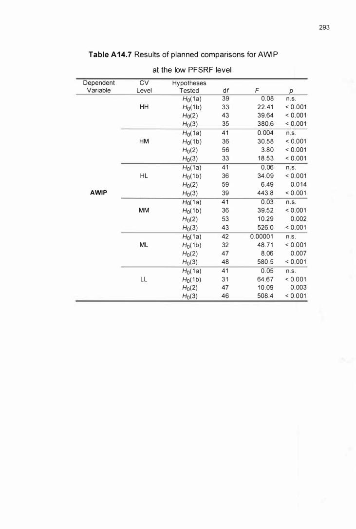
293

Table A 1 4.7 Resu lts of planned comparisons for AWI P

at the low PFSRF level

Dependent CV Hypotheses Variable Level Tested df F P

Ho( 1 a) 39 0.08 n .s . HH Ho( 1 b) 33 22.41 < 0.001

Ho(2) 43 39.64 < 0.001 Ho(3) 35 380.6 < 0.001

Ho( 1 a) 41 0. 004 n .s . HM Ho( 1 b) 36 30.58 < 0.001

Ho(2) 56 3.80 < 0.001 Ho(3) 33 1 8.53 < 0.001

Ho( 1 a) 41 0 .06 n .s . HL Ho( 1 b) 36 34.09 < 0.001

Ho(2) 59 6 .49 0.0 1 4 AWIP Ho(3) 39 443.8 < 0.001

Ho( 1 a) 4 1 0 .03 n .s. MM Ho( 1 b) 36 39.52 < 0.001

Ho(2) 53 1 0.29 0.002 Ho(3) 43 526.0 < 0.001

Ho( 1 a) 42 0.00001 n .s . ML Ho( 1 b) 32 48.7 1 < 0.001

Ho(2) 47 8.06 0.007 Ho(3) 48 580 .5 < 0.001

Ho( 1 a) 41 0 .05 n .s . LL Ho( 1 b) 3 1 64.67 < 0.001

Ho(2) 47 1 0.09 0 .003 Ho(3) 46 508.4 < 0.001

294

Table A 1 4.8 Resu lts of planned comparisons for AFT

at the low PFSRF level

Dependent CV Hypotheses Variable Level Tested df F P

Ho( 1 a) 41 0 .092 n .s. H H Ho( 1 b) 31 28.09 < 0.001

Ho(2) 37 5 1 .07 < 0.001 Ho(3) 34 688 .5 < 0.001

Ho( 1 a) 42 0. 0006 n .s . HM Ho( 1 b ) 33 40.31 < 0.001

Ho(2) 47 20.45 < 0.001 Ho(3) 33 647.85 < 0.001

Ho( 1 a) 4 1 0 .058 n .s . HL Ho( 1 b) 34 45.61 < 0.001

Ho(2) 51 9.22 0.004 AFT Ho(3) 42 854 .3 < 0.001

Ho( 1 a) 42 0.0 1 2 n .s. MM Ho( 1 b) 34 52.5 1 < 0.001

Ho(2) 44 1 4. 1 5 < 0.001 Ho(3) 44 1 067 < 0.001

Ho( 1 a) 42 0.007 n.s . ML Ho( 1 b) 29 63.22 < 0.001

Ho(2) 39 1 0.8 1 0 .002 Ho(3) 55 1 322 < 0.001

Ho( 1 a) 42 0.045 n .s . LL Ho( 1 b) 29 83.85 < 0.001

Ho(2) 39 1 3.89 < 0.001 Ho(3) 52 1 1 24 < 0.001

295

Table A 1 4.9 Resu lts of planned comparisons for ASPTR

at the low PFSRF level

Dependent CV Hypotheses Variable Level Tested df F P

Ho( 1 a) 41 4 .09 0 .05 HH Ho( 1 b) 41 1 1 6 .9 < 0.001

Ho(2) 69 1 4 1 3 1 < 0.001 Ho(3) 22 7869 < 0.001

Ho( 1 a) 39 6 .35 0 .0 16 H M Ho( 1 b) 42 1 06 .8 < 0.001

Ho(2) 66 1 5300 < 0.001 Ho(3) 22 1 4228 < 0.001

Ho( 1 a) 42 6 .32 0.01 6 H L Ho( 1 b) 39 1 1 2 .4 < 0.001

Ho(2) 69 1 2777 < 0.001 ASPTR Ho(3) 24 21 464 < 0.001

Ho( 1 a) 42 1 7.46 < 0.001 MM Ho( 1 b) 36 240. 1 < 0.001

Ho(2) 57 20731 < 0.001 Ho(3) 22 8968 < 0.001

Ho( 1 a) 40 1 2 .06 0.001 ML Ho( 1 b) 40 274.6 < 0.001

Ho(2) 62 1 9707 < 0.001 Ho(3) 22 9673 < 0.001

Ho( 1 a) 4 1 1 2 .23 0.001 LL Ho( 1 b) 42 4 1 4.8 < 0.001

Ho(2) 6 1 2 1 0 1 9 < 0.001 Ho(3) 22 1 20 1 4 < 0.001

296

APPENDIX 1 5

� LIST OF PUBLICATIONS

1 . A paper entitled "Information Flow Model for J IT Shopfloor Control Systems"

has been extended from Section 5 .2 of this thesis and presented to World

Manufacturing Congress (WMC 97) in November 1 997 at Auckland, New

Zealand.

2 . A modifie� version of the content of Chapters 1 -8 of this thesis constituted a

paper entitled " A Simulation Study of the Factors Influencing the Performance

of a Kanban-control led Job Shop", which was presented to the 5th Annual New

Zealand Engineering and Technology Postgraduate Conference at Palmerston

North, New Zealand in November 1 998.

3 . The content o f the first set of experiments of this thesis also provided material for

a paper on "Investigating the Factors Influencing the Shop Performance in a Job

Shop Environment with Kanban-based Production Control", which was

submitted to international Journal of Production Research and is being reviewed.

4. A paper entitled "A Simulation Study of Applying JIT Techniques for Job Shop

Manufacturing" has been condensed from chapters 9- 1 1 of this thesis, and

presented to the lASTED International Conference on Applied Model ling and

Simulation, 1 -3 September, 1 999, Cairns, Australia.