
A RELAXEDHSS PRECONDITIONERFOR SADDLE … RELAXEDHSS PRECONDITIONERFOR SADDLE POINT PROBLEMSFROM...
24
Journal of Computational Mathematics Vol.31, No.4, 2013, 398–421. http://www.global-sci.org/jcm doi:10.4208/jcm.1304-m4209 A RELAXED HSS PRECONDITIONER FOR SADDLE POINT PROBLEMS FROM MESHFREE DISCRETIZATION * Yang Cao School of Transportation, Nantong University, Nantong 226019, China Email: [email protected] Linquan Yao School of Urban Rail Transportation, Soochow University, Suzhou 215006, China Email: [email protected] Meiqun Jiang School of Mathematical Sciences, Soochow University, Suzhou, 215006, China Email: [email protected] Qiang Niu Mathematics and Physics Center, Xi’an Jiaotong-Liverpool University, Suzhou 215123, China Email: [email protected] Abstract In this paper, a relaxed Hermitian and skew-Hermitian splitting (RHSS) preconditioner is proposed for saddle point problems from the element-free Galerkin (EFG) discretization method. The EFG method is one of the most widely used meshfree methods for solving partial differential equations. The RHSS preconditioner is constructed much closer to the coefficient matrix than the well-known HSS preconditioner, resulting in a RHSS fixed-point iteration. Convergence of the RHSS iteration is analyzed and an optimal parameter, which minimizes the spectral radius of the iteration matrix is described. Using the RHSS pre- conditioner to accelerate the convergence of some Krylov subspace methods (like GMRES) is also studied. Theoretical analyses show that the eigenvalues of the RHSS precondi- tioned matrix are real and located in a positive interval. Eigenvector distribution and an upper bound of the degree of the minimal polynomial of the preconditioned matrix are obtained. A practical parameter is suggested in implementing the RHSS preconditioner. Finally, some numerical experiments are illustrated to show the effectiveness of the new preconditioner. Mathematics subject classification: 65F10. Key words: Meshfree method, Element-free Galerkin method, Saddle point problems, Pre- conditioning, HSS preconditioner, Krylov subspace method. 1. Introduction In recent years, meshfree (or meshless) methods have been developed rapidly as a class of potential computational techniques for solving partial differential equations. In the meshfree method, it does not require a mesh to discretize the problem domain, and the approximate solution is constructed entirely on a set of scattered nodes. A lot of meshfree methods have been proposed; see [27] for a general discussion. In this paper, we mainly consider the element- free Galerkin method [11], which is one of the most widely used meshfree methods. * Received July 5, 2012 / Revised version received February 25, 2013 / Accepted April 16, 2013 / Published online July 9, 2013 /
-
Upload
phungtuong -
Category
Documents
-
view
217 -
download
1
Transcript of A RELAXEDHSS PRECONDITIONERFOR SADDLE … RELAXEDHSS PRECONDITIONERFOR SADDLE POINT PROBLEMSFROM...

Journal of Computational Mathematics
Vol.31, No.4, 2013, 398–421.
http://www.global-sci.org/jcm
doi:10.4208/jcm.1304-m4209
A RELAXED HSS PRECONDITIONER FOR SADDLE POINTPROBLEMS FROM MESHFREE DISCRETIZATION*
Yang Cao
School of Transportation, Nantong University, Nantong 226019, China
Email: [email protected]
Linquan Yao
School of Urban Rail Transportation, Soochow University, Suzhou 215006, China
Email: [email protected]
Meiqun Jiang
School of Mathematical Sciences, Soochow University, Suzhou, 215006, China
Email: [email protected]
Qiang Niu
Mathematics and Physics Center, Xi’an Jiaotong-Liverpool University, Suzhou 215123, China
Email: [email protected]
Abstract
In this paper, a relaxed Hermitian and skew-Hermitian splitting (RHSS) preconditioner
is proposed for saddle point problems from the element-free Galerkin (EFG) discretization
method. The EFG method is one of the most widely used meshfree methods for solving
partial differential equations. The RHSS preconditioner is constructed much closer to the
coefficient matrix than the well-known HSS preconditioner, resulting in a RHSS fixed-point
iteration. Convergence of the RHSS iteration is analyzed and an optimal parameter, which
minimizes the spectral radius of the iteration matrix is described. Using the RHSS pre-
conditioner to accelerate the convergence of some Krylov subspace methods (like GMRES)
is also studied. Theoretical analyses show that the eigenvalues of the RHSS precondi-
tioned matrix are real and located in a positive interval. Eigenvector distribution and an
upper bound of the degree of the minimal polynomial of the preconditioned matrix are
obtained. A practical parameter is suggested in implementing the RHSS preconditioner.
Finally, some numerical experiments are illustrated to show the effectiveness of the new
preconditioner.
Mathematics subject classification: 65F10.
Key words: Meshfree method, Element-free Galerkin method, Saddle point problems, Pre-
conditioning, HSS preconditioner, Krylov subspace method.
1. Introduction
In recent years, meshfree (or meshless) methods have been developed rapidly as a class of
potential computational techniques for solving partial differential equations. In the meshfree
method, it does not require a mesh to discretize the problem domain, and the approximate
solution is constructed entirely on a set of scattered nodes. A lot of meshfree methods have
been proposed; see [27] for a general discussion. In this paper, we mainly consider the element-
free Galerkin method [11], which is one of the most widely used meshfree methods.
* Received July 5, 2012 / Revised version received February 25, 2013 / Accepted April 16, 2013 /
Published online July 9, 2013 /
A Relaxed HSS Preconditioner for Saddle Point Problems 399
The EFG method is almost identical to the conventional finite element method (FEM), as
both of them are based on the Galerkin formulation, and employ local interpolation/approximation
to approximate the trial function. The EFG method requires only a set of distributed nodes on
the problem domain, while elements are used in the finite element method. Other key differences
between the EFG method and the FEM method lie in the interpolation methods, integration
schemes and in the enforcement of essential boundary conditions. The EFG method employs
the moving least squares (MLS) approximation method to approximate the trial functions. One
disadvantage of MLS approximation is that the shape functions obtained are lack of Kronecker
delta function property, unless the weight functions used in the MLS approximation are singular
at nodal points. Therefore, the essential boundary conditions in the EFG method can not be
easily and directly enforced. Several approaches have been proposed for imposing the essential
boundary conditions in the EFG method, such as Lagrange multiplier (LM) method [11, 28],
penalty method [33], augmented Lagrangian (AL) method [31], coupled method [22] and so on.
Using independent Lagrange multipliers to enforce essential boundary conditions is common
in structural analysis when boundary conditions can not be directly applied. However, this
method leads to a linear system of saddle point type and increases the number of unknowns.
The penalty method is very simple to be implemented and yields a symmetric positive definite
stiffness matrix, but the penalty parameter must be chosen appropriately. Moreover, the ac-
curacy of the penalty method is less than that of the Lagrange multiplier method in general.
The augmented Lagrangian method uses a generalized total potential energy function to im-
pose essential boundary conditions. The augmented Lagrangian regularization used in the AL
method is composed of the sum of the pure Lagrangian term and the penalty term. In fact, the
AL method combines the LM method and the penalty method, but it leads to a better matrix
structure than the LM method; see discussion in Section 2 and [31]. For other methods stud-
ied for imposing essential boundary conditions in the EFG method; see [22, 27] and references
therein.
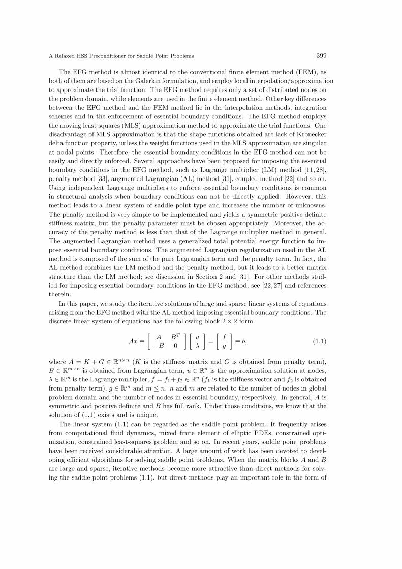
In this paper, we study the iterative solutions of large and sparse linear systems of equations
arising from the EFG method with the AL method imposing essential boundary conditions. The
discrete linear system of equations has the following block 2× 2 form
Ax ≡
[
A BT
−B 0
] [
u
λ
]
=
[
f
g
]
≡ b, (1.1)
where A = K + G ∈ Rn×n (K is the stiffness matrix and G is obtained from penalty term),
B ∈ Rm×n is obtained from Lagrangian term, u ∈ R
n is the approximation solution at nodes,
λ ∈ Rm is the Lagrange multiplier, f = f1+f2 ∈ R
n (f1 is the stiffness vector and f2 is obtained
from penalty term), g ∈ Rm and m ≤ n. n and m are related to the number of nodes in global
problem domain and the number of nodes in essential boundary, respectively. In general, A is
symmetric and positive definite and B has full rank. Under those conditions, we know that the
solution of (1.1) exists and is unique.
The linear system (1.1) can be regarded as the saddle point problem. It frequently arises
from computational fluid dynamics, mixed finite element of elliptic PDEs, constrained opti-
mization, constrained least-squares problem and so on. In recent years, saddle point problems
have been received considerable attention. A large amount of work has been devoted to devel-
oping efficient algorithms for solving saddle point problems. When the matrix blocks A and B
are large and sparse, iterative methods become more attractive than direct methods for solv-
ing the saddle point problems (1.1), but direct methods play an important role in the form of

400 Y. CAO, L.Q. YAO, M.Q. JIANG AND Q. NIU
preconditioners embedded in an iterative frame work. The best known and the oldest methods
are the Uzawa algorithm [14], the inexact Uzawa algorithms [9, 10, 18], the HSS (Hermitian
and skew-Hermitian splitting) algorithms [1–3, 6, 13] and so on. These methods are station-
ary iterative methods. They require much less computer memory than the Krylov subspace
methods in actual implementations. But they are less efficient than the Krylov subspace meth-
ods in general. Unfortunately, Krylov subspace methods also tend to converge slowly when
applied to saddle point problems (1.1), and good preconditioners are needed to achieve rapid
convergence. Preconditioners can be constructed from matrix splitting iterative methods or
matrix factorization. It can also be constructed by special structure of the coefficient matrix.
But the preconditioner should be chosen as close as possible to the coefficient matrix, and the
inverse of preconditioner should be computed easily. In the past few years, much work also
has been devoted to developing efficient preconditioners for saddle point problems. A variety
of preconditioners have been proposed and studied in many papers, such as block diagonal
and block triangular preconditioners [7,19,20,24], constraint preconditioners [8,25], HSS-based
preconditioners [3, 6, 12, 13, 30], dimensional split preconditioners [15, 16], H−matrix precon-
ditioners [17] and so on. In [14], Benzi, Golub and Liesen discussed a selection of numerical
methods and useful preconditioners for saddle point problems. But most existing efficient iter-
ative methods and useful preconditioner are studied for solving saddle point problems arising
from constrained optimization, computational dynamics and so on, there is little discussion on
saddle point problems from meshfree discretization. When n and m are not large, Zheng et al.
proposed a direct method based on Sherman-Morrison formula for solving saddle point problems
from the EFG method [32]. When n and m are large, for solving saddle point problems from
meshfree discretization [32], Leem et al. studied an algebraic multigrid method [26] and Borne
et al. proposed a class of H−matrix preconditioners [17]. For saddle point problems arising
from the EFG method, the class of preconditioners we considered in this paper is a class of HSS
preconditioners, which was proposed by Benzi and Golub in [13]. The HSS preconditioner is
induced by the HSS iterative method, which was first proposed by Bai, Golub and Ng in [4] for
the solution of a broad class of non-Hermitian positive definite linear systems. It was demon-
strated in [4] that the HSS iteration method converges unconditionally to the unique solution
of the non-Hermitian system of linear equations. Then, Benzi and Golub applied the HSS iter-
ation method for solving saddle point problems [13]. They also proved that the HSS iteration
method converges unconditionally to the unique solution of saddle point problems. Due to
its promising performance and elegant mathematical properties, the HSS iteration method has
attracted many researchers’ attention. Algorithmic variants and theoretical analyses of these
HSS iteration methods for saddle point problems have been extensively and deeply discussed
in [1, 3, 6, 12, 13, 21, 23, 30].
In this paper, based on the HSS preconditioner, a relaxed HSS (RHSS) preconditioner is
proposed for saddle point problems (1.1) arising from the EFG discretization method. The
RHSS preconditioner is constructed much closer to the coefficient matrix A than the HSS
preconditioner, resulting in a RHSS fixed-point iteration. Convergence of the RHSS iteration
is analyzed and an optimal parameter, which minimizes the spectral radius of the iteration
matrix is described. Using the RHSS preconditioner to accelerate the convergence of some
Krylov subspace methods (like GMRES) is also studied. Theoretical analyses show that the
eigenvalues of the RHSS preconditioned matrix are real and located in a positive interval.
Eigenvector distribution and an upper bound of the degree of the minimal polynomial of the
preconditioned matrix are obtained. A practical parameter is suggested in implementing the

A Relaxed HSS Preconditioner for Saddle Point Problems 401
RHSS preconditioner. The remainder of the paper is organized as follows. In Section 2, a
model problem and the element free Galerkin method are introduced. Then, in Section 3.1,
the HSS preconditioner is reviewed briefly and a relaxed HSS preconditioner is constructed.
The new preconditioner results in a RHSS fixed-point iteration. In Section 3.2, convergence
of the RHSS iteration is analyzed and an optimal parameter is described. In Section 3.3,
some properties of the RHSS preconditioned matrix are analyzed and a practical parameter
is suggested. Implementation of the preconditioning steps of both HSS preconditioners and
RHSS preconditioners are given in Section 3.4. In Section 4, some numerical experiments are
presented to show the effectiveness of the new preconditioner. Finally, we end this paper with
some conclusions in Section 5.
2. A Model Problem and the Element-free Galerkin Method
The model problem considered is a second-order partial differential equations defined on a
domain Ω ⊂ R2:
−∆u(x) = −(∂2u(x)
∂x2+
∂2u(x)
∂y2
)
= f(x), in Ω, (2.1)
where ∆ is the Laplace operator, u(x) is a unknown function, f(x) is a given function of x and
y, and Ω is a domain enclosed by Γ = ∂Ω = Γu
⋃
Γq with boundary conditions
u = u, on Γu, (2.2)
q(x) =∂u(x)
∂n= q(x), on Γq, (2.3)
where n is the unit outward normal to the boundary Γ, u and q are the prescribed values of
the function u(x) and its normal derivative over the boundary Γ, respectively.
We use the element free Galerkin method to generate discretizations of the model problem
(2.1)-(2.3). As discussed in Section 1, the EFG method is based, as the finite element method,
on an integral formulation. This method, requiring only a set of nodes distributed on the
problem domain, employs the moving least-squares (MLS) approximation for the construction
of the shape functions. In the following, we first give a brief summary of the MLS approximation
scheme, and then present the EFG method for the problem described in (2.1)-(2.3). For details
of the EFG method, see [11, 28].
2.1. The MLS approximation
Consider a sub-domain Ωx, the neighborhood of a point x and denoted as the domain of
definition of the MLS approximation for the trial function at x, which is located in the problem
domain Ω. To approximate the distribution of function u in Ωx, over a number of randomly
located nodes xi, i = 1, · · · , n, the moving least-squares (MLS) approximation uh(x) of u,
∀x ∈ Ωx, can be defined by
uh(x) =
l∑
j=1
pj(x)aj(x) = pT (x)a(x), (2.4)
where pT (x) = [p1(x), · · · , pl(x)] is a complete monomial basis of order l, and aj(x) (j = 1, · · · , l)
are coefficient of the basis functions.

402 Y. CAO, L.Q. YAO, M.Q. JIANG AND Q. NIU
The coefficient vector a(x) can be obtained at any point x by minimizing a weighted discrete
L2 norm, which can be defined as
J(x) =n∑
i=1
wi(x)[pT (xi)a(x)− ui]
2 = [Pa(x)− u]TW [Pa(x)− u], (2.5)
where wi(x) = w(x − xi) is the weight function associated with the node i, with wi(x) > 0 for
all x in the support domain of wi(x), xi denotes the value of x at node i, n is the number of
nodes in Ωx.
The matrices P and W in (2.5) are defined as
P =
p1(x1) p1(x2) · · · p1(xn)
p2(x1) p2(x2) · · · p2(xn)...
.... . .
...
pl(x1) pl(x2) · · · pl(xn)
, W =
w1(x) 0 · · · 0
0 w2(x) · · · 0...
.... . .
...
0 · · · 0 wn(x)
,
and u = [u1, u2, · · · , un]. Here it should be noted that ui(i = 1, 2, · · · , n) are the fictitious
nodal values, not the nodal values in general (see Fig. 1 for a simple one-dimensional case for
the distinction between ui and ui).
Fig. 2.1. The distinction between the nodal values ui of the trial function uh(x) and the
undetermined fictitious nodal values ui in the MLS approximated trial function uh(x).
To find a(x), we obtain the extremum of J in (2.5) by
∂J
∂a= D(x)a(x)− E(x)u = 0, (2.6)
where D(x) = PWPT and E(x) = PW . If D(x) is nonsingular, then from (2.6) we obtain
a(x) = D−1(x)E(x)u.
Substituting a(x) into (2.4), the expression of the local approximation uh(x) is thus
uh(x) = Φ(x)u =n∑
i=1
φi(x)ui, (2.7)
where Φ(x) = φ1(x) · · ·φn(x) is the shape function and
φi(x) =
l∑
j=1
pj(x)[D−1(x)E(x)]ji.

A Relaxed HSS Preconditioner for Saddle Point Problems 403
The derivative of these shape functions can also be obtained
φi,k(x) =
l∑
j=1
[pj,k(D−1E)ji + pj(D
−1,k E +D−1E,k)ji], i = 1, · · · , n,
where
D−1,k = −D−1D,kD
−1,
and the index following a comma is a spatial derivative.
2.2. The EFG formulation
It can be found from above discussion that MLS approximation does not pass through the
data used to fit the curve in general, i.e., it does not have the property of nodal interpolants as
in the FEM, i.e. φi(xj) = δij , where φi(xj) is the shape function corresponding to the node at
xi, evaluated at a nodal point xj , and δij is the Kronecker delta. Thus the essential boundary
conditions can not be imposed directly in the EFG method. In this paper, the augmented
Lagrangian method [31] is used to enforce the essential boundary conditions.
In Cartesian coordinate system, the functional corresponding to equation (2.1) associated
to the boundary conditions (2.2) and (2.3) is given by
Π(u) =1
2
∫
Ω
(
(∂u
∂x)2 + (
∂u
∂y)2 − 2uf
)
dΩ−
∫
Γq
qudΓ
+
∫
Γu
λ(u − u)dΓ +β
2
∫
Γu
(u− u)T (u− u)dΓ, (2.8)
where λ is the Lagrange multiplier and β is the penalty parameter, they are used to impose the
essential boundary conditions. The Lagrange multiplier λ can be expressed by
λ(s) =∑
i
Ni(s)λi, (2.9)
where Ni(s) is a Lagrange interpolation, s is the arc length along the boundary Γu, λi is the
Lagrange multiplier at the ith node located at the essential boundary.
The necessary condition for (2.8) to reach its minimum yields
δuΠ(u, λ) =
∫
Ω
[(δux)Tux + (δuy)
Tuy − fT δu]dΩ−
∫
Γq
qδudΓ
+∫
Γu
λT δudΓ + β∫
Γu
[(δu)Tu− (δu)T u]dΓ = 0,(2.10)
δλΠ(u, λ) =
∫
Γu
δλ(u − u)dΓ = 0, (2.11)
where δu and δλ are the test functions, (δu)x and (δu)y (ux and uy) are the derivatives of δu(u)
in terms of x and y, respectively.
Substituting (2.7) and (2.9) into (2.11) and (2.11), then integrating, we obtain the following
discrete linear system of equations
Ax ≡
[
A BT
−B 0
] [
u
λ
]
=
[
f
g
]
≡ b, (2.12)

404 Y. CAO, L.Q. YAO, M.Q. JIANG AND Q. NIU
where
A =
∫
Ω
GTGdΩ + β
∫
Ω
ΦTΦdΓ, B =
∫
Γu
NTΦdΓ, (2.13)
f =
∫
Γq
ΦT qdΓ + β
∫
Γu
ΦT udΓ, g = −
∫
Γu
NT udΓ, (2.14)
and
G =
[
∂φ1
∂x· · · ∂φn
∂x∂φ1
∂y· · · ∂φn
∂y
]
, Φ =[
φ1 · · · φn
]
, N =[
N1 · · · Nm
]
.
It should be noted that u in (2.12) is u in fact. It is also the fictitious nodal value, not
the nodal value in general. Once (2.12) has been solved, we can use (2.7) to get approximate
values for every point of interest. Using the augmented Lagrangian method to enforce essential
boundary conditions in the EFG method has some advantages [31], such as high precision,
good stability and so on. Moreover, the blocks of discrete linear system (2.12) have some
nice properties, such as A is symmetric and positive definite, B has full row rank. If there is
no penalty used, i.e. using the Lagrange multipliers only, then A is symmetric and positive
semi-definite in general. In the following, we will study the iterative solution of linear system
(2.12). However, the coefficient matrix A is ill-conditioned in general for large n and m. Many
iterative methods (for example splitting iterative methods, Krylov subspace methods) tend to
converge very slowly when applied to saddle point system (2.12). In the next section, a relaxed
HSS preconditioner will be proposed to achieve rapid convergence when some Krylov subspace
methods (such as GMRES) are used. The corresponding iterative method is also studied.
3. The Relaxed HSS (RHSS) Preconditioner
In this section, we first review briefly the HSS iterative method and introduce the HSS
preconditioner, for details; see [4,13,30]. Then a relaxed HSS preconditioner will be constructed.
Some properties of the RHSS preconditioned matrix are studied.
3.1. The HSS preconditioner and the RHSS preconditioner
From the structure of the saddle point system (1.1), we know that the coefficient matrix A
naturally possesses the Hermitian and skew-Hermitian splitting
A = H+ S,
where
H =1
2(A+AT ) =
[
A 0
0 0
]
, S =1
2(A−AT ) =
[
0 BT
−B 0
]
.
Let α > 0 be a given parameter, I be the (appropriately dimensioned) identity matrix. It is
easy to see that αI +H and αI + S are both nonsingular matrices. Consider two splittings of
A
A = (αI +H)− (αI − S) and A = (αI + S)− (αI −H).
Then we can obtain the following HSS iterative method for solving saddle point problem (2.12).

A Relaxed HSS Preconditioner for Saddle Point Problems 405
Algorithm 3.1. (The HSS iteration method)
Given an initial guess x0, for k = 0, 1, 2, · · · , until xk converges, compute
(αI +H)xk+ 1
2 = (αI − S)xk + b,
(αI + S)xk+1 = (αI −H)xk+ 1
2 + b,
where α is a given positive constant.
It has been studied in [13] that the HSS iteration method is convergent unconditionally to
the unique solution of the saddle point problem (2.12). In matrix-vector form, the above HSS
iteration can be equivalently rewritten as
xk+1 = Γαxk +Nαb, (3.1)
where
Γα = (αI + S)−1(αI −H)(αI +H)−1(αI − S),
Nα = 2α(αI + S)−1(αI +H)−1.
Here, Γ(α) is the iteration matrix of the HSS iteration. In fact, (3.1) also results from the
splitting
A = PHSS −NHSS
of the coefficient matrix A, with
PHSS =1
2α(αI +H)(αI + S), and NHSS =
1
2α(αI −H)(αI − S).
We note that Γα = P−1HSSNHSS , N (α) = P−1
HSS , and PHSS can be served as a preconditioner,
called the HSS preconditioner, to the system of linear equations (1.1). It should be noted that
the pre-factor 12α in the HSS preconditioner PHSS has no effect on the preconditioned system.
For the purpose of analysis, we can take the HSS preconditioner as
PHSS =1
α(αI +H)(αI + S). (3.2)
By performing the matrix multiplication on the right-hand side of (3.2), it follows that PHSS
has the following structure
PHSS =1
α
[
A+ αI 0
0 αI
] [
αI BT
−B αI
]
=
[
A+ αI BT + 1αABT
−B αI
]
. (3.3)
It follows from (2.12) and (3.3) that the difference between the preconditioner PHSS and the
coefficient matrix A is given by
RHSS = PHSS −A =
[
αI 1αABT
0 αI
]
. (3.4)

406 Y. CAO, L.Q. YAO, M.Q. JIANG AND Q. NIU
From (3.4), we can see that when α tends to zero, the same as the diagonal blocks. However,
the off-diagonal block becomes unbound. Hence, we should choose an ideal α to balance the
weight of both parts (see [30]).
To obtain an improved invariant of the HSS preconditioner, we hope that the preconditioner
PHSS is as close as possible to the coefficient matrix A. Based on this idea, we propose a relaxed
HSS preconditioner as follows
PRHSS =1
α
[
A 0
0 αI
] [
αI BT
−B 0
]
=
[
A 1αABT
−B 0
]
. (3.5)
We can easily see that the difference between PRHSS and A is given by
RRHSS = PRHSS −A =
[
0 ( 1αA− I)BT
0 0
]
. (3.6)
Compared with the matrix RHSS , diagonal blocks of the matrix RRHSS become zero ma-
trices, while the nonzero off-diagonal becomes ( 1αA− I)BT . This means that the relaxed HSS
preconditioner PRHSS should be closer to the coefficient matrix A than the original HSS precon-
ditioner PHSS . This observation suggests that PRHSS will lead to a better preconditioner than
PHSS , since it gives a better approximation of the coefficient matrix A. It should be noted
that the RHSS preconditioner PRHSS no longer relates to an alternating direction iteration
method, but this fact is of no consequence when PRHSS is used as a precodntioner for Krylov
subspace method like GMRES. In fact, the RHSS preconditioner PRHSS can be obtained by
the following splitting of the coefficient matrix A
A =
[
A 1αABT
−B 0
]
−
[
0 ( 1αA− I)BT
0 0
]
≡ PRHSS −RRHSS , (3.7)
which results in the following RHSS iteration method.
Algorithm 3.2. (The RHSS iteration method)
Let α be a given positive constant. Let [u0, λ0] be an initial guess vector. For k = 0, 1, 2, · · · ,
until certain stopping criteria satisfied, compute
[
A 1αABT
−B 0
] [
uk+1
λk+1
]
=
[
0 ( 1αA− I)BT
0 0
] [
uk
λk
]
+
[
f
g
]
.
From (3.5), the RHSS iteration method can be solved by two steps. We may first solve the
system of linear equations with the first coefficient matrix in (3.5), then solve the system of
linear equations with the second coefficient matrix in (3.5). Details of implementation steps are
studied in Section 3.4.
3.2. Analysis of the RHSS iteration
In this section, we deduce the convergence property of the RHSS iteration method and the
optimal parameter α. Note that the iteration matrix of the RHSS iteration method is
Γ = P−1RHSSRRHSS =
[
A 1αABT
−B 0
]−1 [0 ( 1
αA− I)BT
0 0
]
. (3.8)

A Relaxed HSS Preconditioner for Saddle Point Problems 407
Let ρ(Γ) denote the spectral radius of Γ. Then the RHSS iteration method converges if and
only if ρ(Γ) < 1. Let
P1 =
[
A 0
0 αI
]
, P2 =
[
αI BT
−B 0
]
.
It is easy to check that
P−11 =
[
A−1 0
0 1αI
]
, P−12 =
[
1αI − 1
αBT (BBT )−1B −BT (BBT )−1
(BBT )−1B α(BBT )−1
]
. (3.9)
Then the iteration matrix Γ can be rewritten by
Γ = αP−12 P−1
1 RRHSS =
[
0 (BT (BBT )−1B − I)(A−1 − 1αI)BT
0 I − α(BBT )−1BA−1BT
]
.
From the above expression, we know that the spectral radius of the RHSS iteration matrix Γ is
ρ(Γ) = max1≤i≤m
|1− αµi|, (3.10)
where µi (1 ≤ i ≤ m) is the ith eigenvalue of (BBT )−1(BA−1BT ). In fact, the spectral radius
(3.10) is similar to a spectral radius when a stationary Richardson iteration applied to the
following linear system
(BBT )−1
2 (BA−1BT )(BBT )−1
2 x = b.
Let µ1 and µm be the largest and smallest eigenvalues of (BBT )−1(BA−1BT ), respec-
tively. If A is symmetric and positive definite, so is (BBT )−1
2 (BA−1BT )(BBT )−1
2 . Since
(BBT )−1(BA−1BT ) is similar to (BBT )−1
2 (BA−1BT )(BBT )−1
2 , the smallest and largest eigen-
values of (BBT )−1
2 (BA−1BT )(BBT )−1
2 are µm and µ1, respectively. It is well known that
Richardson’s iteration converges for all α such that
0 < α <2
µ1.
Furthermore, the spectral radius ρ(Γ) is minimized by taking
αopt =2
µ1 + µm
. (3.11)
Same results are true for the RHSS iteration method. We summarize them in the following
theorem.
Theorem 3.1. Let A ∈ Rn×n be a symmetric and positive definite matrix, B ∈ R
m×n have
full row rank, and let α be a positive constant. Let ρ(Γ) be the spectral radius of the RHSS
iteration matrix. Then
ρ(Γ) = max1≤i≤m
|1− αµi|,
where µi is the ith eigenvalue of (BBT )−1(BA−1BT ). Let µ1 and µm be the largest and smallest
eigenvalues of (BBT )−1(BA−1BT ), respectively. If α satisfies
0 < α <2
µ1,

408 Y. CAO, L.Q. YAO, M.Q. JIANG AND Q. NIU
then the RHSS iteration method is convergent. The optimal α, which minimizes the spectral
radius ρ(Γ), is given by
αopt =2
µ1 + µm
.
The corresponding optimal spectral radius is
ρopt(Γ) =µ1 − µm
µ1 + µm
.
In general, the asymptotic rate of convergence of the stationary iteration is governed by the
spectral radius of the iteration matrix Γ, so it makes sense to try to choose the parameter α so as
to make ρ(Γ) as small as possible. In Theorem 3.1, the optimal parameter and its corresponding
optimal spectral radius are presented. From the expression of the optimal spectral radius, we
can see that if µ1 is very close to µm, then ρopt(Γ) is very close to zero and fast convergence
will be obtained. But if µ1 ≫ µm, then ρopt(Γ) is very close to 1 and the RHSS iteration
will converge very slowly. Fortunately, the rate of convergence can be greatly improved by
Krylov subspace acceleration. In other words, using PRHSS as a preconditioner for some Krylov
subspace methods (such as GMRES) may be a good choice. In fact, we can rewrite the RHSS
iteration in correction form:
xk+1 = xk + P−1RHSSrk, rk = b−Axk. (3.12)
This will be useful when we consider Krylov subspace acceleration. Moreover, knowing con-
vergent condition of the RHSS iteration method is very important, since it implies that the
spectrum of the preconditioned matrix lies entirely in a circle centered at (1, 0) with unity
radius which is a desirable property for Krylov subspace acceleration. Using the optimal pa-
rameter αopt, eigenvalues of preconditioned matrix may be more cluster than that of other
cases. To obtain the optimal parameter αopt, we need to solve the extreme eigenvalues of
(BBT )−1(BA−1BT ). This is a difficult task. In the next section, some properties of the pre-
conditioned matrix are studied and a practical parameter is suggested in implementing the
RHSS preconditioner.
3.3. Analysis of the preconditioned matrix P−1RHSSA
The RHSS iteration method is a stationary iteration. It is very simple and very easy to
implement. But if µ1 ≫ µm, the convergence of the RHSS iteration is typically too slow for the
method to be competitive even with the optimal choice of the parameter α. In this section, we
propose using the Krylov subspace method like GMRES to accelerate the convergence of the
iteration.
It follows from (3.12) that the linear system Ax = b is equivalent to the linear system
(I − Γ)x = P−1RHSSAx = c,
where c = P−1RHSSb. This equivalent (left-preconditioned) system can be solved with GMRES.
Hence, the matrix PRHSS can be seen as a preconditioner for GMRES. Equivalently, we can
say that GMRES is used to accelerate the convergence of the splitting iteration applied to
Ax = b [29]. In general, a clustered spectrum of the preconditioned matrix P−1RHSSA often
translates in rapid convergence of GMRES. In the following, we will deduce the eigenvalue
distribution of the preconditioned matrix P−1RHSSA. Besides, the eigenvector distribution and
an upper bound of the minimal polynomial of the preconditioned matrix are also discussed.

A Relaxed HSS Preconditioner for Saddle Point Problems 409
Theorem 3.2. The eigenvalues of the preconditioned matrix P−1RHSSA are given by 1 with
multiplicity at least n. The remaining eigenvalues are positive real and located in
[αµm, αµ1],
where µ1 and µm are the maximum and the minimum eigenvalues of matrix (BBT )−1BA−1BT .
Proof. From (3.9), we have
P−1RHSSA = P−1
RHSS(PRHSS −RRHSS)
= I − P−1RHSSRRHSS = I − αP−1
2 P−11 RRHSS
= I − α
[
1αI − 1
αBT (BBT )−1B −BT (BBT )−1
(BBT )−1B α(BBT )−1
] [
A−1 0
0 1αI
] [
0 ( 1αA− I)BT
0 0
]
= I −
[
I −BT (BBT )−1B −αBT (BBT )−1
α(BBT )−1B α2(BBT )−1
] [
0 ( 1αI −A−1)BT
0 0
]
= I −
[
0 (BT (BBT )−1B − I)(A−1 − 1αI)BT
0 I − α(BBT )−1BA−1BT
]
=
[
I (I −BT (BBT )−1B)(A−1 − 1αI)BT
0 α(BBT )−1BA−1BT
]
. (3.13)
Eq. (3.13) implies that the eigenvalues of the preconditioned matrix P−1RHSSA are given by
1 with multiplicity at least n, the remaining nonunit eigenvalues are the nonunit eigenvalues
of α(BBT )−1BA−1BT . Since BBT and BA−1BT are symmetric and positive definite, and α
is a positive parameter, the eigenvalues of α(BBT )−1BA−1BT are positive real. Denote µ1
and µm be the maximum and the minimum eigenvalues of matrix (BBT )−1BA−1BT , then the
remaining nonunit eigenvalues of the preconditioned matrix P−1RHSSA are located in [αµm, αµ1].
This completes the proof.
From Theorem 3.1, we know that eigenvalues of the preconditioned matrix are 1 with mul-
tiplicity at least n, and the remaining eigenvalues are real and located in a positive interval,
which is related to the parameter α. Like all parameter based iterative methods, it is very dif-
ficult to obtain the optimal choice of the parameter. The optimal parameter αopt (3.11), which
minimizes the spectral radius of the RHSS iteration matrix Γ, can be used. In this case, all
the eigenvalues of the preconditioned matrix P−1RHSSA lie entirely in a circle centered at (1, 0)
with unity radius which is a desirable property for Krylov subspace acceleration. To obtain the
optimal parameter αopt, we need to solve the extreme eigenvalues of (BBT )−1(BA−1BT ). This
should be a difficult task. Fortunately, from Theorem 3.2, we know that the parameter has no
effect on the ratio of the interval [αµm, αµ1]. This means that α = 1 may be a good choice
for the RHSS preconditioner. In the next section, some numerical experiments will show this
observation. It should be noted that α = 1 may be not a good choice for the RHSS iteration
method, since the RHSS iteration method may be divergence in this case.
In the following, we turn to study the eigenvector distribution and an upper bound of the
degree of the minimal polynomial of the preconditioned matrix P−1RHSSA.
Theorem 3.3. Let the RHSS preconditioner be defined in (3.5), then the preconditioned matrix
P−1RHSSA has n+ i+ j linearly independent eigenvectors. There are

410 Y. CAO, L.Q. YAO, M.Q. JIANG AND Q. NIU
• n eigenvectors of the form[
uT 0T]T
that correspond to the eigenvalue 1.
• i (1 ≤ i ≤ m) eigenvectors of the form[
uT vT]T
arising from ( 1αA − I)BT v = 0 for
which i vectors v are linearly independent and the eigenvalue is 1.
• j (1 ≤ j ≤ m) eigenvectors of the form[
uT vT]T
that correspond to nonunit eigen-
values.
Proof. The form of the eigenvectors of the preconditioned matrix P−1RHSSA can be derived
by considering the following generalized eigenvalue problem
[
A BT
−B 0
] [
u
v
]
= θ
[
A 1αABT
−B 0
] [
u
v
]
, (3.14)
where θ is an eigenvalue of the preconditioned matrix P−1RHSSA and
[
uT vT]T
is the corre-
sponding eigenvector. Expanding (3.14) out, we obtain
Au +BT v = θAu +θ
αABT v, (3.15)
(1 − θ)Bu = 0. (3.16)
Eq. (3.16) implies that either θ = 1 or Bu = 0. If θ = 1, then (3.15) can be rewritten as
( 1
αA− I
)
BT v = 0. (3.17)
Eq. (3.17) is trivially satisfied by v = 0, and hence there are n linearly independent eigenvectors
of the form[
uT 0T]T
associated with the eigenvalue 1. If there exists any v 6= 0 which
satisfies (3.17), then there will be i (1 ≤ i ≤ m) linearly independent eigenvectors of the form[
uT vT]T
, where the components v arise from (3.17).
If θ 6= 1, then from (3.15), we have
u =1
1− θ
( θ
αI −A−1
)
BT v. (3.18)
Substituting (3.18) into (3.16), we get
αBA−1BT v = θBBT v. (3.19)
For this case, it must be v 6= 0. Otherwise, from (3.18) we get u = 0, a contradiction. If there
exists any v 6= 0 which satisfies (3.19), then there will be j (1 ≤ j ≤ m) linearly independent
eigenvectors of the form[
uT vT]T
that correspond to nonunit eigenvalues. Thus, the form
of the eigenvectors are obtained. Let
a(1) =[
a(1)1 · · · a
(1)n
]T
, a(2)=[
a(2)1 · · · a
(2)i
]T
, a(3)=[
a(3)1 · · · a
(3)j
]T
,
be three vectors. To show that the n+ i+ j eigenvectors of the preconditioned matrix P−1RHSSA

A Relaxed HSS Preconditioner for Saddle Point Problems 411
are linearly independent, we need to show that
[
u(1)1 · · · u
(1)n
0 · · · 0
]
a(1)1...
a(1)n
+
[
u(2)1 · · · u
(2)i
v(2)1 · · · v
(2)i
]
a(2)1...
a(2)i
+
[
u(3)1 · · · u
(3)j
v(3)1 · · · v
(3)j
]
a(3)1...
a(3)j
=
0...
0
, (3.20)
implies that the vectors a(k) (k = 1, 2, 3) are zero vectors. Recalling that in (3.20) the first
matrix arises from the case θk = 1 (k = 1, · · · , n), the second matrix from the case θk = 1
(k = 1, · · · , i), and the last matrix from the case θk 6= 1 (k = 1, · · · , j). Multiplying (3.20) by
P−1RHSSA, gives
[
u(1)1 · · · u
(1)n
0 · · · 0
]
a(1)1...
a(1)n
+
[
u(2)1 · · · u
(2)i
v(2)1 · · · v
(2)i
]
a(2)1...
a(2)i
+
[
u(3)1 · · · u
(3)j
v(3)1 · · · v
(3)j
]
θ1a(3)1...
θja(3)j
=
0...
0
. (3.21)
Subtracting (3.20) from (3.21), we obtain
[
u(3)1 · · · u
(3)j
v(3)1 · · · v
(3)j
]
(θ1 − 1)a(3)1
...
(θj − 1)a(3)j
=
0...
0
.
Since the fires matrix above are j linearly independent vectors and the eigenvalues θk 6= 1
(k = 1, · · · , j), we have a(3)k = 0 (k = 1, · · · , j). We also have linear independence of v
(2)k
(k = 1, · · · , i), and thus a(2)k = 0 (k = 1, · · · , i). Thus, (3.20) can be simplified to
[
u(1)1 · · · u
(1)n
0 · · · 0
]
a(1)1...
a(1)n
=
0...
0
.
Because of the linear independence of u(1)k (k = 1, · · · , n), we have a
(1)k = 0 (k = 1, · · · , n).
Thus, the proof is complete.
Theorem 3.4. Let the RHSS preconditioner be defined in (3.5), then the degree of the minimal
polynomial of the preconditioned matrix P−1RHSSA is at most m+1. Thus, the dimension of the
Krylov subspace K(P−1RHSSA, b) is at most m+ 1.

412 Y. CAO, L.Q. YAO, M.Q. JIANG AND Q. NIU
Proof. By (3.13), we know that the preconditioned matrix P−1RHSSA takes the form
P−1RHSSA =
[
I Θ2
0 Θ1
]
, (3.22)
where Θ1 = α(BBT )−1BA−1BT ∈ Rm×m and Θ2 = (I − BT (BBT )−1B)(A−1 − 1
αI)BT ∈
Rn×m.
From the eigenvalue distribution studied in Theorem 3.2, it is evident that the characteristic
polynomial of the preconditioned matrix P−1RHSSA is
(P−1RHSSA− I)n
m∏
i=1
(P−1RHSSA− µiI).
Expanding the polynomial (P−1RHSSA− I)
m∏
i=1
(P−1RHSSA− µiI) of degree m+ 1, we obtain
(P−1RHSSA− I)
m∏
i=1
(P−1RHSSA− µiI) =
0 Θ2
m∏
i=1
(Θ1 − µiI)
0 (Θ1 − I)m∏
i=1
(Θ1 − µiI)
.
Since µi (i = 1, · · · ,m) are also the eigenvalues of Θ1 ∈ Rm×m, thus we have
m∏
i=1
(Θ1 − µiI) = 0.
Therefore, we obtain the degree of the minimal polynomial of the preconditioned matrix
P−1RHSSA is at most m+1. From [29, Proposition 6.1], we know that the degree of the minimal
polynomial is equal to the dimension of the corresponding Krylov subspace K(P−1RHSSA, b) (for
general b). So, the dimension of the Krylov subspace K(P−1RHSSA, b) is also at most m + 1.
Thus, we complete the proof.
It directly follows from Theorem 3.4 that any Krylov subspace iterative method with an
optimality or Galerkin property, for example GMRES [29], will terminate in at most m + 1
iterations with the solution to a linear system of the form (2.12) if the RHSS preconditioner
PRHSS is used. It should be noted that for the linear system of equations (2.12), the dimension
m is related to the number of nodes located at the essential boundary and n is related to the
number of nodes located in global problem domain. In general, m is much less than n. It seems
that the RHSS preconditioner PRHSS should be very effective for the saddle point problems
arising from the element free Galerkin discretization method.
3.4. Implementation
In this section, for saddle point problems (2.12) we use the relaxed HSS preconditioner
PRHSS to derive a preconditioning implementation in a Krylov subspace iterative method,
such as GMRES. To compare with the RHSS preconditioner, the preconditioning steps of the
HSS preconditioner PHSS are also given.
Since the pre-factor 1αin the RHSS preconditioner PRHSS has no effect on the preconditioned
system, application of the RHSS preconditioner with GMRES, we need to solve the linear system
of the form[
A 0
0 αI
] [
αI BT
−B 0
]
z = r,
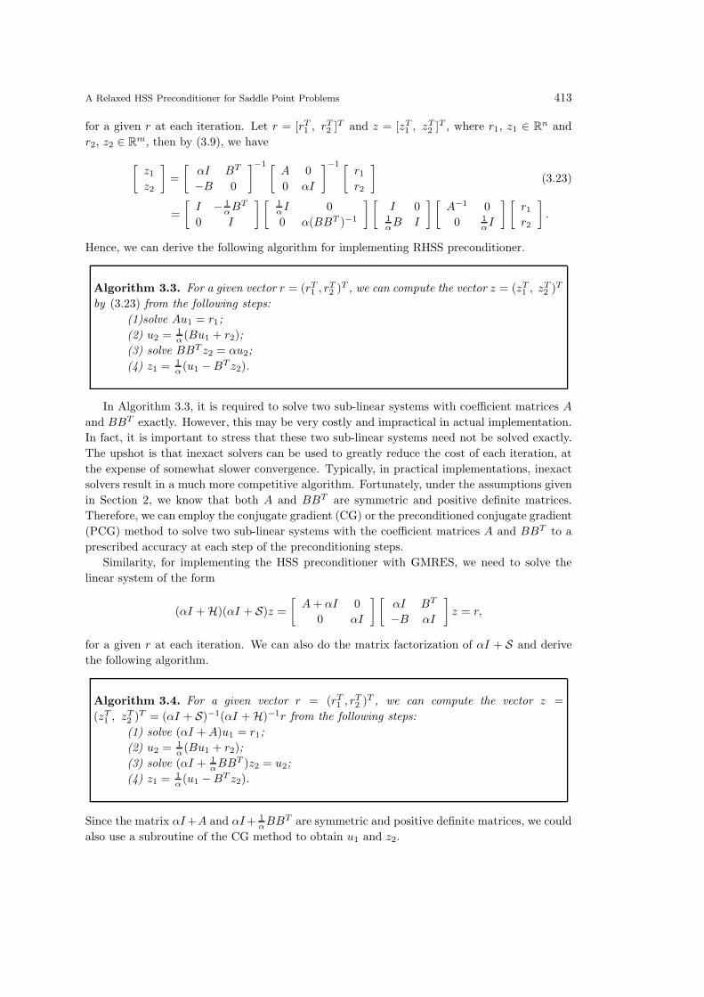
A Relaxed HSS Preconditioner for Saddle Point Problems 413
for a given r at each iteration. Let r = [rT1 , rT2 ]T and z = [zT1 , zT2 ]
T , where r1, z1 ∈ Rn and
r2, z2 ∈ Rm, then by (3.9), we have
[
z1z2
]
=
[
αI BT
−B 0
]−1 [A 0
0 αI
]−1 [r1r2
]
(3.23)
=
[
I − 1αBT
0 I
] [
1αI 0
0 α(BBT )−1
] [
I 01αB I
] [
A−1 0
0 1αI
] [
r1r2
]
.
Hence, we can derive the following algorithm for implementing RHSS preconditioner.
Algorithm 3.3. For a given vector r = (rT1 , rT2 )
T , we can compute the vector z = (zT1 , zT2 )
T
by (3.23) from the following steps:
(1)solve Au1 = r1;
(2) u2 = 1α(Bu1 + r2);
(3) solve BBT z2 = αu2;
(4) z1 = 1α(u1 −BT z2).
In Algorithm 3.3, it is required to solve two sub-linear systems with coefficient matrices A
and BBT exactly. However, this may be very costly and impractical in actual implementation.
In fact, it is important to stress that these two sub-linear systems need not be solved exactly.
The upshot is that inexact solvers can be used to greatly reduce the cost of each iteration, at
the expense of somewhat slower convergence. Typically, in practical implementations, inexact
solvers result in a much more competitive algorithm. Fortunately, under the assumptions given
in Section 2, we know that both A and BBT are symmetric and positive definite matrices.
Therefore, we can employ the conjugate gradient (CG) or the preconditioned conjugate gradient
(PCG) method to solve two sub-linear systems with the coefficient matrices A and BBT to a
prescribed accuracy at each step of the preconditioning steps.
Similarity, for implementing the HSS preconditioner with GMRES, we need to solve the
linear system of the form
(αI +H)(αI + S)z =
[
A+ αI 0
0 αI
] [
αI BT
−B αI
]
z = r,
for a given r at each iteration. We can also do the matrix factorization of αI + S and derive
the following algorithm.
Algorithm 3.4. For a given vector r = (rT1 , rT2 )
T , we can compute the vector z =
(zT1 , zT2 )T = (αI + S)−1(αI +H)−1r from the following steps:
(1) solve (αI +A)u1 = r1;
(2) u2 = 1α(Bu1 + r2);
(3) solve (αI + 1αBBT )z2 = u2;
(4) z1 = 1α(u1 −BT z2).
Since the matrix αI+A and αI+ 1αBBT are symmetric and positive definite matrices, we could
also use a subroutine of the CG method to obtain u1 and z2.

414 Y. CAO, L.Q. YAO, M.Q. JIANG AND Q. NIU
0 0.1 0.2 0.3 0.4 0.5 0.6 0.7 0.8 0.9 10
0.1
0.2
0.3
0.4
0.5
0.6
0.7
0.8
0.9
1
x
y
Typical nodes distribution and background cells for example 4.1
Fig. 4.1. Example 4.1: 21× 21 regular nodes distribution and 10× 10 background cells.
From Algorithm 3.3 and Algorithm 3.4, we can see that two steps are different. In the first
step and the third step of Algorithm 3.3, we need to solve linear systems with coefficient matrix
A and BBT , respectively, while in the first and the third step of Algorithm 3.4, we need to
solve linear systems with coefficient matrix αI + A and αI + 1α(BBT ), respectively. This is a
simple modification, but it may result in good convergence. In the next section, some numerical
experiments are illustrated to show this observation.
4. Numerical Experiments
In this section, two numerical examples are illuatrated to show the effectiveness of the RHSS
iteration method (Algorithm 3.2) and the RHSS preconditioner (3.5) for saddle point problem
(2.12), from the point of view of both number of total iteration steps (denoted by ‘IT ’) and
elapsed CPU time in seconds (denoted by ‘CPU ’). In actual computations, all runs are started
from the initial vector (uT0 , λ
T0 ) = [0, · · · , 0]T , and terminated if the current iterations satisfy
ERR= ||rk||2/||r0||2 ≤ 10−8 (where rk = b −Axk is the residual at the kth iteration) or if the
number of prescribed iteration kmax = 1000 is exceeded. All runs are performed in MATLAB
7.0 on an Intel core i5 (2G RAM) Windows 7 system.
Model problems are discretized by the EFG method. Using the augmented Lagrangian
method to impose essential boundary conditions leads to saddle point problems (2.12). The
linear basis pT = [1, x, y] and the cubic spline weight function [28] are used to construct MLS
shape functions. To obtain integrals in (2.13) and (2.14), background cells will be used in this
paper. It should be noted that these background cells are independent of nodes distribution.
For each background cell, 4× 4 Gauss points are used. For each computational point (node or
Gauss point), rectangular influence domain is adopted. The radius of each influence is taken as
γ× dc, where γ is the scale and dc is the average node distance. In this paper, we take γ = 2.5.
Taking the penalty β = 10 in (2.13) and (2.14) to ensure that (1,1) block A of saddle point
matrix is positive definite.
Example 4.1. The first numerical example is the Poisson equation
−∆u = 2π2sinπxcosπy in Ω = [0, 1]× [0, 1]

A Relaxed HSS Preconditioner for Saddle Point Problems 415
Table 4.1: Values of m, n and the order of A for Example 4.1.
Nodes 21×21 41×41 61×61 81×81
n 441 1681 3721 6561
m 42 82 122 162
n+m 483 1763 3843 6723
Table 4.2: Parameters for Example 4.1.
Nodes 21×21 41×41 61×61 81×81
2/µ1 0.67203 0.65661 0.65368 0.65264
αopt 0.54657 0.53623 0.53425 0.53355
[αµm, αµ1] [0.37338, 1.62662] [0.36665,1.63335] [0.36541,1.63457] [0.36494,1.63506]
with boundary conditions
u = 0 on x = 0 and x = 1,
∂u
∂n= 0 on y = 0 and y = 1.
For this example, we have two essential boundaries, i.e., x = 0 and x = 1. Other two
boundaries, i.e., y = 0 and y = 1, are natural boundaries. To discritize the problem domain
Ω = [0, 1]× [0, 1], we take four regular nodes distribution, i.e., 21× 21, 41× 41, 61× 61, 81× 81.
For each node distribution, 10 × 10, 20 × 20, 30 × 30 and 40 × 40 background cells are used
to obtain integrals, respectively. A typical 21 × 21 nodes distribution and the corresponding
10 × 10 background cells are plotted in Fig. 4.1. The orders of saddle point matrices A are
listed in Table 4.1.
In Table 4.2, we list the upper bound of the convergent interval and the optimal parame-
ters for the RHSS iteration method, and the bound of eigenvalues of the RHSS preconditioned
matrix P−1RHSSA with optimal αopt. From Table 4.2, we can see that all eigenvalues of the pre-
conditioned matrix P−1RHSSA are located in (0, 2) if optimal parameters were used. In Table 4.3,
we list the numbers of iteration steps and the computing CPU times (in seconds) with respect to
RHSS iteration method with optimal parameter (Algorithm 3.2), GMRES (no preconditioning,
denote by I), HSS preconditioned GMRES (with α = 1, 0.1, 0.01) and RHSS preconditioned
GMRES (with α = 1, αopt). From Table 4.3, we can see that
• RHSS iteration converges very fast for solving saddle point problems (2.13) when optimal
parameter is used. Without preconditioning, GMRES converges very slowly. If the HSS
preconditioner or the RHSS preconditioner were used, the preconditioned GMRES method
converges very fast.
• For the RHSS preconditioned GMRES, the numbers of iteration steps and the elapsed
CPU times are almost the same when α = 1 and α = αopt are used. But for the HSS
preconditioned GMRES, the numbers of iteration steps and the elapsed CPU times vary
greatly when different α are used.
• The optimal parameter αopt, which minimizes the spectral radius of corresponding itera-
tion matrix, is not the optimal parameter for the RHSS preconditioner. But this optimal
parameter can get very good numerical results.

416 Y. CAO, L.Q. YAO, M.Q. JIANG AND Q. NIU
0 0.2 0.4 0.6 0.8 1 1.2 1.4 1.6 1.8 214
14.2
14.4
14.6
14.8
15
15.2
15.4
15.6
15.8
16
α
IT
RHSS preconditioning steps vs α
0 0.2 0.4 0.6 0.8 1 1.2 1.4 1.6 1.8 20
50
100
150
200
250
α
IT
HSS preconditioning steps vs α
Fig. 4.2. Example 4.1: the effect of α: RHSS preconditioning steps vs α (left); HSS precondi-
tioning steps vs α (right).
In order to study the effect of preconditioners with respect to parameters, Fig. 4.2 plots
RHSS preconditioning steps and HSS preconditioning steps (varying α from 0.01 to 2) when
41× 41 nodes are used. From Fig. 4.2, we can see that the parameter α does not influence the
RHSS preconditioning steps greatly, while it influences the HSS preconditioning steps greatly.
It seems that in the RHSS preconditioner α = 1 may be a good choice. But for the HSS
preconditioner, we should compute optimal parameters. If inappropriate parameter were used,
the preconditioned GMRES may converge slowly. In general, finding optimal parameter α in
the HSS preconditioner is a very difficult task.
Fig. 4.3 plots eigenvalue distribution of the saddle point matrixA (without preconditioning),
the HSS preconditioned matrix P−1HSSA (with α = 0.01), the RHSS preconditioned matrix
P−1RHSSA (with α = 1) and the RHSS preconditioned matrix P−1
RHSSA (with α = αopt) when
n +m = 1763. From Fig. 4.3, we can see that the eigenvalues of preconditioned matrices are
more cluster than those of original matrix and good convergence may be obtained.
Table 4.3: Numerical results of GMRES and preconditioned GMRES for Example 4.1.
Nodes 21×21 41×41 61×61 81×81
RHSS iterationIT 28 28 25 24
CPU 0.204 0.332 0.9222 1.891
IIT 153 304 403 479
CPU 0.496 1.456 6.465 12.770
PHSS(α=1)IT 106 207 271 316
CPU 0.114 0.953 3.221 7.201
PHSS(α=0.1)IT 52 92 115 131
CPU 0.064 0.313 0.968 2.057
PHSS(α=0.01)IT 26 33 44 56
CPU 0.041 0.144 0.375 0.835
PRHSS(αopt)IT 11 14 14 14
CPU 0.018 0.073 0.204 0.367
PRHSS(α=1)IT 11 15 15 16
CPU 0.039 0.098 0.199 0.383

A Relaxed HSS Preconditioner for Saddle Point Problems 417
0 500 1000 1500 200010
−5
100
105
eigenvalue number
eige
nval
ueNo preconditioning
0 500 1000 1500 200010
−3
10−2
10−1
100
eigenvalue number
eige
nval
ue
HSS preconditioning (α=0.01)
0 500 1000 1500 20000
1
2
3
4
eigenvalue number
eige
nval
ue
RHSS preconditioning (α=1)
0 500 1000 1500 20000
0.5
1
1.5
2
eigenvalue number
eige
nval
ue
RHSS preconditioning (αopt
)
Fig. 4.3. Eigenvalue distribution for Example 4.1.
0 0.2 0.4 0.6 0.8 1 1.2 1.452
54
56
58
60
62
64
66
68
α
IT
RHSS preconditioning steps vs α
0 0.2 0.4 0.6 0.8 1 1.2 1.4100
150
200
250
300
350
400
α
IT
HSS preconditioning steps vs α
Fig. 4.4. Example 4.2: the effect of α: RHSS preconditioning steps vs α (left); HSS precondi-
tioning steps vs α (right).
Example 4.2. The second numerical example is the Stokes problem: find u and p such that
−ν∆u+p = f , in Ω,
· u = g, in Ω,
u = 0, on ∂Ω,∫
Ω p(x)dx = 0.
(4.1)
where Ω = [0, 1]× [0, 1] ⊂ R2, ∂Ω is the boundary of Ω, ν stands for the viscosity scalar, ∆ is

418 Y. CAO, L.Q. YAO, M.Q. JIANG AND Q. NIU
the componentwise Laplace operator, u = (uT , vT )T is a vector-valued function representing
the velocity, and p is a scalar function representing the pressure.
For this example, we have four essential boundaries, i.e., x = 0, x = 1, y = 0, y = 1.
There is no natural boundary. Nodes distribution and background cells are taken the same as
Example 4.1. The viscosity scalar ν is taken as 1. The pressure p is taken at the center of each
background cell. The orders of saddle point matrices A are listed in Table 4.4.
Table 4.4: Values of m, n and the order of A for Example 4.2.
Nodes 21×21 41×41 61×61 81×81
n 882 3362 7442 13122
m 184 564 1144 1924
n+m 1066 3926 8586 15046
Table 4.5: Parameters for Example 4.2.
Nodes 21×21 41×41 61×61 81×81
2/µ1 0.22975 0.06153 0.02776 0.01571
αopt 0.22828 0.06142 0.02773 0.01569
[αµm, αµ1] [0.01277,1.98723] [0.00344,1.99656] [0.00155,1.99845] [0.00088,1.99912]
Table 4.6: Numerical results of GMRES and preconditioned GMRES for Example 4.2.
Nodes 21×21 41×41 61×61 81×81
IIT 469 835 985 −
CPU 2.685 27.029 66.226 −
PHSS(α=1)IT 377 644 743 955
CPU 1.653 15.257 41.833 117.693
PHSS(α=0.1)IT 191 336 446 479
CPU 0.502 4.877 17.495 36.358
PHSS(α=0.01)IT 175 243 252 302
CPU 0.442 2.974 7.347 18.084
PRHSS(αopt)IT 53 70 85 98
CPU 0.124 0.616 1.906 4.479
PRHSS(α=1)IT 54 68 82 92
CPU 0.144 0.620 1.866 4.228
In Table 4.5, we list the optimal parameters used in the RHSS preconditioner and the
corresponding positive interval for Example 4.2. Table 4.6 lists the numbers of iteration steps
and the computing CPU times (in seconds) with respect to GMRES (no preconditioning), HSS
preconditioned GMRES (with α = 1, 0.1, 0.01) and RHSS preconditioned GMRES (with α =
1, αopt). Fig. 4.4 plots RHSS preconditioning steps, and HSS preconditioning steps (varying α
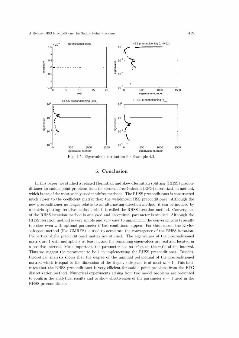
from 0.01 to 1.1) when n+m = 1066. Fig. 4.5 depicts eigenvalue distribution of the saddle point
matrix A (without preconditioning), the HSS preconditioned matrix P−1HSSA (with α = 0.01),
the RHSS preconditioned matrix P−1RHSSA (with α = 1) and the RHSS preconditioned matrix
P−1RHSSA (with α = αopt) when n+m = 1066.
From these tables and figures, we can also see that using preconditioners can accelerate the
convergence greatly, especially when suitable parameters are used. Moreover, the parameter α
in the RHSS preconditioner is less sensitive than the parameter α in the HSS preconditioner.
For the preconditioner PRHSS , α = 1 is also a practical choice.
A Relaxed HSS Preconditioner for Saddle Point Problems 419
0 5 10 15 20−1.5
−1
−0.5
0
0.5
1
1.5x 10
−4
real
imag
inar
yNo preconditioning
0 500 1000 150010
−6
10−4
10−2
100
eigenvalue number
eige
nval
ue
HSS preconditioning (α=0.01)
0 500 1000 150010
−2
10−1
100
101
eigenvalue number
eige
nval
ue
RHSS preconditioning (α=1)
0 500 1000 150010
−2
10−1
100
101
eigenvalue number
eige
nval
ue
RHSS preconditioning (αopt
)
Fig. 4.5. Eigenvalue distribution for Example 4.2.
5. Conclusion
In this paper, we studied a relaxed Hermitian and skew-Hermitian splitting (RHSS) precon-
ditioner for saddle point problems from the element-free Galerkin (EFG) discretization method,
which is one of the most widely used meshfree methods. The RHSS preconditioner is constructed
much closer to the coefficient matrix than the well-known HSS preconditioner. Although the
new preconditioner no longer relates to an alternating direction method, it can be induced by
a matrix splitting iterative method, which is called the RHSS iteration method. Convergence
of the RHSS iteration method is analyzed and an optimal parameter is studied. Although the
RHSS iteration method is very simple and very easy to implement, the convergence is typically
too slow even with optimal parameter if bad conditions happen. For this reason, the Krylov
subspace method (like GMRES) is used to accelerate the convergence of the RHSS iteration.
Properties of the preconditioned matrix are studied. The eigenvalues of the preconditioned
matrix are 1 with multiplicity at least n, and the remaining eigenvalues are real and located in
a positive interval. Most important, the parameter has no effect on the ratio of the interval.
Thus we suggest the parameter to be 1 in implementing the RHSS preconditioner. Besides,
theoretical analysis shows that the degree of the minimal polynomial of the preconditioned
matrix, which is equal to the dimension of the Krylov subspace, is at most m + 1. This indi-
cates that the RHSS preconditioner is very efficient for saddle point problems from the EFG
discretization method. Numerical experiments arising from two model problems are presented
to confirm the analytical results and to show effectiveness of the parameter α = 1 used in the
RHSS preconditioner.

420 Y. CAO, L.Q. YAO, M.Q. JIANG AND Q. NIU
Acknowledgments. The authors express their thanks to the referees for the comments and
constructive suggestions, which were valuable in improving the quality of the manuscript. This
work is supported by the National Natural Science Foundation of China(11172192) and the
National Natural Science Pre-Research Foundation of Soochow University (SDY2011B01).
References
[1] Z.-Z. Bai, Optimal parameters in the HSS-like methods for saddle point problems, Numer. Linear
Algebra Appl., 16 (2009), 447-479.
[2] Z.-Z. Bai and G.H. Golub, Accelerated Hermitian and skew-Hermitian splitting iteration methods
for saddle-point problems, IMA J. Numer. Anal., 27 (2007), 1-23.
[3] Z.-Z. Bai, G.H. Golub, C.-K. Li, Convergence properties of preconditioned Hermitian and skew-
Hermitian splitting methods for non-Hermitian positive semidefinite matrices, Math. Comput., 76
(2007), 287-298.
[4] Z.-Z. Bai, G.H. Golub and M.K. Ng, Hermitian and skew-Hermitian splitting methods for non-
Hermitian positive definite linear systems, SIAM J. Matrix Anal. Appl., 24 (2003), 603-626.
[5] Z.-Z. Bai, G.H. Golub and M.K. Ng, On successive-overrelaxation acceleration of the Hermitian
and skew-Hermitian splitting iterations, Numer. Linear Algebra Appl., 14 (2007), 319-335.
[6] Z.-Z. Bai, G.H. Golub and J.-Y. Pan, Preconditioned Hermitian and skew-Hermitian splitting
methods for non-Hermitian positive semidefinite linear systems, Numer. Math., 98 (2004), 1-32.
[7] Z.-Z. Bai and M.K. Ng, On inexact preconditioners for nonsymmetric matrices, SIAM J. Sci.
Comput., 26 (2005), 1710-1724.
[8] Z.-Z. Bai, M.K. Ng and Z.-Q. Wang, Constraint preconditioners for symmetric indefinite matrices,
SIAM J. Matrix Anal. Appl., 31 (2009), 410-433.
[9] Z.-Z. Bai, B.N. Parlett and Z.-Q. Wang, On generalized successive overrelaxation methods for
augmented linear systems, Numer. Math., 102 (2005) 1-38.
[10] Z.-Z. Bai and Z.-Q. Wang, On parameterized inexact Uzawa methods for generalized saddle point
problems, Linear Algebra Appl., 428 (2008), 2900-2932.
[11] T. Belytschko, Y.Y. Lu and L. Gu, Element-free Galerkin methods, Int. J. Numer. Meth. Engrg.,
37 (1994), 229-256.
[12] M. Benzi, M.J. Gander and G.H. Golub, Optimization of the Hermitian and skew-Hermitian
splitting iteration for saddle-point problems, BIT, 43 (2003), 881-900.
[13] M. Benzi and G.H. Golub, A preconditioner for generalized saddle point problems, SIAM J. Matrix
Anal. Appl., 26 (2004), 20-41.
[14] M. Benzi, G.H. Golub and J. Liesen, Numerical solution of saddle point problems, Acta Numer.,
14 (2005), 1-137.
[15] M. Benzi, and X.-P. Guo, A dimensional split preconditioner for Stokes and linearized Navier-
Stokes equations, Appl. Numer. Math., 61 (2011), 66-76.
[16] M. Benzi, M.K. Ng, Q. Niu and Z. Wang, A relaxed dimensional fractorization preconditioner for
the incompressible Navier-Stokes equations, J. Comput. Phys., 230 (2011), 6185-6202.
[17] S.L. Borne, S. Oliveira and F. Yang, H-matrix preconditioners for symmetric saddle-point systems
from meshfree discretization, Numer. Linear Algebra Appl., 15 (2008), 911-924.
[18] Y. Cao, M.-Q. Jiang and L.-Q. Yao, New choices of preconditioning matrices for generalized
inexact parameterized iterative methods, J. Comput. Appl. Math., 235 (2010), 263-269.
[19] Y. Cao, M.-Q. Jiang and Y.-L. Zheng, A splitting preconditioner for saddle point problems, Numer.
Linear Algebra Appl., 18 (2011), 875-895.
[20] Y. Cao, M.-Q. Jiang and Y.-L. Zheng, A note on the positive stable block triangular preconditioner
for generalized saddle point problems, Appl. Math. Comput., 218 (2012) 11075-11082.
[21] Y. Cao, W.-W. Tan and M.-Q. Jiang, A generalization of the positive-definite and skew-Hermitian
splitting iteration, Numer. Algebra Control Optimization, 2 (2012), 811-821.

A Relaxed HSS Preconditioner for Saddle Point Problems 421
[22] Y. Cao, L.-Q. Yao and Y. Yin, New treatment of essential boundary conditions in EFG method
by coupling with RPIM, Acta Mech. Solida Sinica, To appear.
[23] M.-Q. Jiang and Y. Cao, On local Hermitian and skew-Hermitian splitting iteration methods for
generalized saddle point problems, J. Comput. Appl. Math., 231 (2009), 973-982.
[24] M.-Q. Jiang, Y. Cao and L.-Q. Yao, On parameterized block triangular preconditioners for gen-
eralized saddle point problems, Appl. Math. Comput., 216 (2010), 1777-1789.
[25] C. Keller, N.I.M. Gould and A.J. Wathen, Constraint preconditioning for indefinite linear systems,
SIAM J. Matrix Anal. Appl., 21 (2000), 1300-1317.
[26] K.H. Leem, S. Oliveira and D.E. Stewart, Algebraic multigrid (AMG) for saddle point systems
from meshfree discretizations, Numer. Linear Algebra Appl., 11 (2004) 293-308.
[27] G.-R. Liu and Y.-T. Gu, An introduction to meshfree methods and their programming, Nether-
land: Springer; 2005.
[28] F.Z. Loua1, N. Na1t-Sa1d and S. Drid, Implementation of an efficient element-free Galerkin
method for electromagnetic computation, Eng. Anal. Boundary Elem., 31 (2007), 191-199.
[29] Y. Saad, Iterative Methods for Sparse Linear Systems(2nd edn), SIAM: Philadelphia, 2003.
[30] V. Simoncini and M. Benzi, Spectral properties of the Hermitian and skew-Hermitian splitting
preconditioner for saddle point problems, SIAM J. Numer. Anal., 27 (2007), 1-23.
[31] G. Ventura, An augmented Lagrangian approach to essential boundary conditions in meshless
methods, Int. J. Numer. Meth. Engng., 53 (2002), 825-842.
[32] H. Zheng and J.-L. Li, A practical solution for KKT systems, Numer. Algor., 46 (2007) 105-119.
[33] T. Zhu and S.N. Atluri, A modified collocation method and a penalty formulation for enforcing
the essential boundary conditions in the element free Galerkin method, Comput. Mech., 21 (1998),
211-222.