1  

 

 

A Regional Perspective on the Economic

Resiliency of Central and East European

Economies

 

Josef C. Brada

Arizona State University

and

CERGE- Economic Institute of the Czech Academy of Sciences and Charles University

Paweł Gajewski

University of Łodz

Ali Kutan

Southern Illinois University – Edwardsville

This version December 2018

2  

Abstract

In this paper we examine resiliency, the ability to absorb and recover from economic

shocks, in 199 Nuts-3 regions in Central and Eastern Europe following the 2008 global

financial crisis. We find that regional productivity has a clear influence on the ability to resist

and recover from shocks. More productive regions fare better than do regions with low output

per worker. Moreover, regions that resist shocks well also recover to a greater extent. Finally,

we find strong positive regional spillovers, which means that regions tend to form clusters of

high-performing and low-performing areas, a process that exacerbates regional income

disparities.

JEL Classification Numbers: J61, J63, P25, R11, R12

Key Words: Regional resiliency, Central and Eastern Europe, economic recovery, industrial employment, regional economics

3  

I. Introduction

In part due to the slow recovery from the global financial crisis of 2008, there has been

a renewed interest in the concepts of economic resiliency, the ability of economies to absorb

economic shocks and to recover from them. The traditional approach in macroeconomics was

that downturns are temporary and that the economy would return more or less quickly to the

long-term growth path of GDP as idle workers and capital were put back to use. In the literature

on resiliency, this is called the single-equilibrium approach, where a system is seen as returning

to the status ex ante. The aftermath of the 2008 crisis put this traditional view into question.

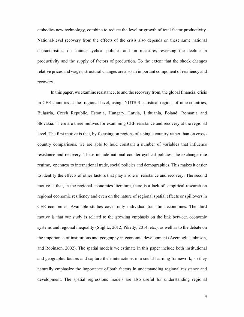
Figure 1 shows that the world’s major economies reacted differently to the initial shock, at least

quantitatively if not qualitatively, and none of them were able to recover to the pre-crisis trend

of real GDP. Thus, macroeconomic resiliency came to be seen not as a return to the pre-crisis

state or growth path, but rather as the adaptation to the new circumstances in which the

economy finds itself as a result of the crisis. Ball (2014), Haltmeier (2012), Martin et al. (2014)

and Reinhart and Rogoff (2014), using somewhat different methodologies and data sets, all

demonstrate intercountry differences in both the resistance to shocks and in the recovery from

them. Central and Eastern Europe (CEE) appears to have been particularly hard hit by the

crisis, and recovery was less dynamic than it was in the older EU countries (Figure 2).

At the national level, resiliency to shocks depends on the openness of the economy, to

the country’s exchange rate regime, to the structure of production, and to national policies to

deal with the effects of the shock. Return to the status quo ex ante is difficult because shocks

create shortfalls in labor, capital and technology related to the decline in output. Reduced

investment during the downturn lowers the capital to labor ratio, workers leave the labor force

thus reducing the labor force participation ratio and, if unemployed, they cease to acquire

human capital from learning by doing and their existing skills atrophy. Research and

development also decline, and, together with lower levels of investment in capital that

4  

embodies new technology, combine to reduce the level or growth of total factor productivity.

National-level recovery from the effects of the crisis also depends on these same national

characteristics, on counter-cyclical policies and on measures reversing the decline in

productivity and the supply of factors of production. To the extent that the shock changes

relative prices and wages, structural changes are also an important component of resiliency and

recovery.

In this paper, we examine resistance, to and the recovery from, the global financial crisis

in CEE countries at the regional level, using NUTS-3 statistical regions of nine countries,

Bulgaria, Czech Republic, Estonia, Hungary, Latvia, Lithuania, Poland, Romania and

Slovakia. There are three motives for examining CEE resistance and recovery at the regional

level. The first motive is that, by focusing on regions of a single country rather than on cross-

country comparisons, we are able to hold constant a number of variables that influence

resistance and recovery. These include national counter-cyclical policies, the exchange rate

regime, openness to international trade, social policies and demographics. This makes it easier

to identify the effects of other factors that play a role in resistance and recovery. The second

motive is that, in the regional economics literature, there is a lack of empirical research on

regional economic resiliency and even on the nature of regional spatial effects or spillovers in

CEE economies. Available studies cover only individual transition economies. The third

motive is that our study is related to the growing emphasis on the link between economic

systems and regional inequality (Stiglitz, 2012; Piketty, 2014, etc.), as well as to the debate on

the importance of institutions and geography in economic development (Acemoglu, Johnson,

and Robinson, 2002). The spatial models we estimate in this paper include both institutional

and geographic factors and capture their interactions in a social learning framework, so they

naturally emphasize the importance of both factors in understanding regional resistance and

development. The spatial regressions models are also useful for understanding regional

5  

inequality issues. For instance, Martin et al., (2016, p. 583) state that “the study of regional

cyclical resistance and recoverability is … integral to understanding long-run patterns of

uneven regional development”. Our study should be seen in the context of growing post-

transition income disparities between regions in the CEE economies. Capital cities and the

regions close to them have gained significantly in population and, more important, in per capita

income, while peripheral regions in these countries have experienced declines in per capita

income, thus contributing to growing income inequality in the CEE economies. Hence, our

study further sheds some light on inequality issues from a long-run perspective and beyond a

national level, and also complements Stiglitz (2012), Piketty (2014) and other related studies.

The remainder of the paper is organized as follows: Section II reviews the literature on

regional resiliency, on spatial regression models and on the literature of regional

responsiveness in CEE. Section III explains the data sources and main variables of interest.

Stylized facts on regional resistance and recovery in CEE are presented in Section IV, which

also explains how we capture regional spillovers. Section V explains the construction of

indexes used in our regression models. Sections VI and VII provide the specification of the

regression model and present and discuss the parameter estimates, respectively. Section VIII

concludes.

 

II. Literature Survey

Studies on regional resiliency in economics have examined regional resiliency in the

face of ecological disasters, demographic and technological change, shifts in demand and

globalization. The Cambridge Journal of Regions, Economy and Society (2010), and the

Journal of Regional Science (2012) have published special issue on regional resiliency that

cover many of the key conceptual issues. This literature survey consists of three parts. In the

first part, we summarize the literature regarding different concepts of resiliency. In the second

6  

part, different spatial models employed in the literature are briefly introduced. The last part

provides an overview of empirical studies using spatial models of regional resiliency.

II.1 Defining regional resiliency

Early studies of regional resiliency focused on understanding the process and patterns

of resistance to change in the face of shocks. As the concept is used in different fields, including

engineering, ecology, geography, sociology, etc., what signifies regional resiliency is shaped

by their corresponding fields (Christopherson, Michie, and Tyler, 2010; Hassink, 2010;

Hudson, 2010; Pike, Dawley, and Tomaney, 2010; Simmie and Martin, 2010; Wolfe, 2010).

The literature provides three concepts of resiliency: single-equilibrium (engineering

resiliency), multiple-equilibrium (path dependent or ecological resiliency), and adaptive

resiliency.

According to the single-equilibrium approach, a regional economy facing a shock

should return to its pre-shock equilibrium level. This approach assumes a stable, long-run

relationship among the key economic variables driving economic performance and the free and

flexible operation of factor markets. Resiliency is then measured in terms of how quickly a

regional variable such as output, employment, etc. returns to the pre-shock equilibrium

(Pendall, Foster and Cowell, 2010; Pike et al., 2010; Fingleton, Garretsen and Martin, 2012).

According to the path-dependency approach, the performance of a regional economy is

assumed to be determined by economic forces (investment, migration, relative price changes,

etc.) that also change as the result of the shock. Consequently, in the face of shocks, a region

is unlikely to return to its previous pre-shock equilibrium path or state. Resiliency is then

measured by the success of affected regions in moving from the suboptimal immediate post-

shock state to a new equilibrium. In this view, resiliency is associated with flexibility and the

ability to make adjustments to new circumstances. Such adjustments depend on the capacity of

local firms, workers, market institutions and governments to undertake changes in the structure

7  

of economic activities. Such shifts generate multiple possible equilibrium states, depending on

how regional parameters change (Hassink, 2010; Pike et al, 2010, Wolfe, 2010; Doran and

Fingleton, 2018).

The third definition, adaptive resiliency, extends the path-dependency approach and

views regional resiliency as a complex and evolving process, involving social learning by

workers, firms, and institutions as they try to overcome uncertainty in the face of a shock

(Hansink, 2010; Hudson, 2010; Pike at al., 2010). According to this view, resiliency to shocks

is determined by, and determines, factors such as industrial structure (specialization vs

diversity), institutions, agglomeration economies and others (Doran and Fingleton, 2014;

Martin, Sunley, Gardiner and Tyler, 2016; and Doran and Fingleton, 2018). In other words,

adaptive resiliency assumes an endogenous, two-way causal relationship between economic

outcomes and shocks and their underlying regional determinants. Martin and Sunley (2016)

argue that regional resiliency includes four consecutive phases: risk, resistance, reorientation

and recoverability, and they all depend on the size, nature and duration of shocks. In the risk

phase, regions recognize that they are vulnerable to internal and external shocks. The resistance

stage captures how firms, economic sectors, institutions and other key players resist shocks and

adjust, and then adapt to the shocks (i.e., the reorientation step). The recoverability step

captures fruits of making the required adjustments and the degree to which regions recover

from the shock. Martin et al., (2016, p. 583) state that “the study of regional cyclical resistance

and recoverability is … integral to understanding long-run patterns of uneven regional

development”.

II.2. A brief review of spatial regression models

Lesage and Fischer (2008) developed spatial regression models to test for resiliency in

a regional growth setting. Their empirical framework is based on specifying a full spatial

8  

Durbin Model (SDM) and discussing its variants. The starting point for the development of

their model is the following simple pooled linear regression:

yit = xit β+ εit (1)

where the variable y represents a vector of observed values of the dependent variable, for

example regional output or employment, and vector x is a vector of k independent variables. i

is an index for the cross-sectional dimension (regions) while t is an index that captures the time

dimension. β is a vector that captures the impact of the independent variables on the dependent

variable. The error term, ε, has a zero mean and constant variance and is independently and

identically distributed.

Equation (1) does not include any spatial effects. To capture the impact of potential

spillovers from one region to another on the dependent variable, Lesage and Fischer (2008)

specify the following SDM model:

yit = ρWyjt + xit β1 +Wxjt β2 + εit (2)

Equation 2 indicates that the link between y and x in region i is not only a function of

independent variables in region i but also of the explanatory variables for other regions, j.1

Hence, the SDM model shows the way in which region i is influenced by developments in

region j through spatial spillover effects. W is called the spatial weight matrix and its elements

represent the spatial dependency among the observations. In some cases this spillover effect is

limited to spillovers from adjacent regions so the effect is captured by a dummy variable thsat

takes a value of 1 if two regions share a border and a value of zero otherwise (i.e. a contiguity

matrix) or by other measures of distance between regions. In particular, the term Wyjt captures

the characteristics of neighboring or related regions and ρ, called the spatially lagged dependent

variable, shows the economic significance of neighboring independent variables on the

                                                            1 For example, other regions may mean all other regions in a country or contiguous regions only.

9  

dependent variable. A positive and significant value of ρ indicates positive spatial dependency

in that the dependent variable in region i is positively related to developments in related regions

j. Note that ρ must be less than 1. On the other hand, the Wx matrix represents explanatory

variables from related regions with β2 capturing their economic significance for the dependent

variable in region i. Finally, β1 captures the impact of the independent variables in region i on

the dependent variable in the same region (i.e., own effects).

Lesage and Fischer (2008) suggest two additional spatial models that are nested within

the SDM model, namely, the spatial autoregressive (SAR) model (when β2=0 and ρ≠0) and the

spatial error (SEM) model (when β2 = -β1ρ). Thus, while the SDM yields unbiased parameter

estimates because it is a generalization of the SAR and SEM models, testing for the above

parameter restrictions can improve effciency of the estimates.2 Consequently, it is of some

value to select the correct type of spatial model. To do so, Lesage and Pace (2009) and Elshort

(2009) suggest that the SDM model should be estimated first and then be tested against the

alternative SAR and SEM models by checking the validity of the above coefficient restrictions.

Once the correct model is chosen, Lesage and Pace (2009) recommend estimating the direct,

indirect and total effects for each independent variable. The direct effect captures the impact

of explanatory variables in region i on the dependent variable. The indirect effect represents

the spillovers from related regions. How these effects are measured is discussed below.

II.3 Review of empirical spatial studies

There is little research on regional economic resiliency of CEE economies. Much of the

study the regions of the CEE countries focus on regional income dispersion and on regional

spatial effects or spillovers. Regarding the latter, Elshort, Blien and Wolf (2007) estimate a

spatial wage curve for Eastern German districts during 1993-1999 and report that estimates of

                                                            2 The SDM model also handles possible endogeneity bias resulting from both simultaneity and omitted variables.

10  

unemployment elasticities are sensitive to the inclusion of spatially correlated error terms in

their specifications. Baltagi and Rokicki (2014) also estimate the spatial wage curve for Poland

using individual data from the Polish Labor Force Survey at the NUTS-2 level, and they report

significant spatial unemployment spillovers across regions.

Kholodin et al. (2012) find significant convergence of income levels among high-

income regions located near each other. This suggests the existence of the kind of spatial effects

discussed in the previous section. In CEE counties, there seems to have been a lack of

convergence in regional incomes. The capital cities and their neighboring regions have

prospered in all CEE countries, also suggesting strong regional spillovers, but there are also

regions in each country where performance is relatively poor. 

III. Data and variables

The data used in this study refer to NUTS-3 statistical regions in nine Central and

Eastern European Countries (CEECs: Bulgaria, Czechia, Estonia, Hungary, Latvia, Lithuania,

Poland, Romania and Slovakia. The main source of data is Eurostat, but, in some cases, national

sources (most notably the Polish Local Database, BDL from the Central Statistical Office,

GUS) were also used to fill missing observations. Eurostat also provided the spatial data in the

form of shapefiles with geographical coordinates, which are used in the article for the purpose

of tracking spatial dependency and spillovers.

While we make use of the temporal information to capture the impact of pre-crisis

regional features on regional resistance to the crisis, as well as the role of post-shock

adjustments for the recovery, the models themselves are cross-sectional over the 199 NUTS-3

regions in our sample. Following Martin (2012) and Martin et al. (2016), we decompose

resiliency into its two dimensions: resistance (the ability of a regional economy to resist or

withstand an external shock) and recoverability (its ability to recover after the shock).

11  

For measures of resistance we focus on a region’s non-agricultural employment. We

choose this variable for several reasons. First, non-agricultural employment is likely to be more

sensitive to changes in economic conditions especially those due to external shocks.

Agricultural employment, much of it self-employment, is less likely to respond to changes in

economic conditions. Thus, regions with large agrarian populations would give the appearance

of greater resistance merely due to the mix of agricultural and industrial employment. Second,

changes in industrial production are easier to implement in the short run than are changes in

the nature of agricultural production. Finally, policies to deal with shocks are largely directed

toward the industrial sector.

Regional resistance is calculated in the following way. First, the non-agricultural

employment change in region i, between the pre-crisis peak and the subsequent trough is

 

𝑥, ,… , ,

, ,∗ 100%  (3) 

 where 𝑒 is the non-agricultural employment in region i in year 20xx. Thus, if region i loses

employment as a result of the shock, 𝑥 < 0. In this way we allow for differences in the years

in which the crisis began to be felt in different regions and also for differences in the years in

which the effects of the crisis on employment reached their maximum. An examination of the

data on employment showed that the years of peak employment were sometime between 2006

and 2008 and the trough occurred sometime between 2008 and 2013.

In the second step, a raw index of regional resistance is calculated, using the country in

which the region is located, c, as the baseline so that :

𝑟𝑒𝑠𝑟𝑎𝑤| |

(4)

where 𝑥 is the decline in employment from peak to trough in country c.

Since 𝑥 0: 

12  

𝑟𝑒𝑠𝑟𝑎𝑤

1∈ 0,1

00

when there was no decline in employment during the crisiswhen the region is more resilient than its country of origin

when the region is as resilient as its country of originwhen the region is less resilient than its country of origin

 

 

Comparing 𝑟𝑒𝑠𝑟𝑎𝑤 indices for regions belonging to different countries makes little

sense as country-specific variations of employment during and after the crisis influence the

denominator. If, for example, a country’s total employment declined only marginally during

the crisis, the regional resistance index could be extremely large even for moderate declines of

employment. Therefore, the resistance measures are standardized to zero mean and unit

variance within each country by Equation 5:

𝑟𝑒𝑠                                                                     (5) 

where 𝜇 is mean and 𝛿 is the standard deviation of regional resilience indicator values

within the country. This standardization permits comparability of regional resistance across

countries and abstracts from national resistance. Consequently,

𝑟𝑒𝑠 00

if the region was more resistant than an average region within the countryif the region was less resistant than an average region within the country

Our approach means that we weight all regions equally so they have an equal impact on the

country average.3

We follow a similar procedure to calculate measures of regional recoverability (𝑟𝑒𝑐 ),

which we define as the relative extent to which regional economies recovered, in terms of non-

agricultural employment, between the trough of the crisis (anytime between 2008 and 2013)

and the end of our sample, i.e. 2015.4

                                                            3 In practice the regions vary from 150,000 to 800,000 inhabitants. 4 2014 for Romanian regions, because data for 2015 were found to be unreliable.   

13  

𝑦∗ , ,…

, ,…∗ 100% (6)

  

𝑟𝑒𝑐𝑟𝑎𝑤                                                             (7) 

 

𝑟𝑒𝑐                                                             (8) 

 

Note that the values of 𝑟𝑒𝑐𝑟𝑎𝑤 , unlike 𝑟𝑒𝑠𝑟𝑎𝑤 , are not bounded, i.e.:

𝑟𝑒𝑐𝑟𝑎𝑤 and 𝑟𝑒𝑐

00

if the region had better recoverability than an average region in the countryif the region had worse recoverability than an average region in the country

 

IV. Stylized Facts About CEE Resistance and Recoverability

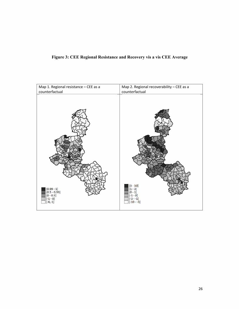
A broader picture of regional resistance and recoverability is obtained by using the

Central and Eastern European (CEE) aggregate non-agricultural employment change as a

counterfactual, thus substituted for 𝑥 and 𝑦 , respectively. By using the CEE average job loss

or gain, the relative resiliency of countries is reflected in their regional resistance and recovery

variables. Maps 1 and 2 in Figure 3 illustrate these indices, which are not stripped of country-

wide factors. Note that the resilience indicator here has the same properties as 𝑟𝑒𝑠𝑟𝑎𝑤 . Several

regions in Poland, as well as the central and suburban parts of the capital city of Bucharest (in

Romania) did not experience a decline of employment during the crisis whatsoever. Regions

that proved resistant relative to the average CEE experience (those with dark shading) were

generally clustered in Poland, Czechia and Slovakia, which reflected the relatively good

performance of these economies at the onset of the crisis, as compared to other CEECs. This

better performance may be due to the flexible exchange rate of the former two countries and to

all three countries’ close integration into the supply networks of multinational firms. On the

other hand, most regions in the Baltic States, but also in Bulgaria and Romania (excluding

Bucharest), showed little resistance to the crisis, the former likely due to their exchange rate

14  

arrangements. The most successful recovery was observed in a belt of Polish regions running

from the north-central to eastern part of the country, in Estonia and Hungary, followed by

Lithuania. In both of these maps, Poland stands out as the most heterogenous country,

encompassing both well- and poorly-performing regions.

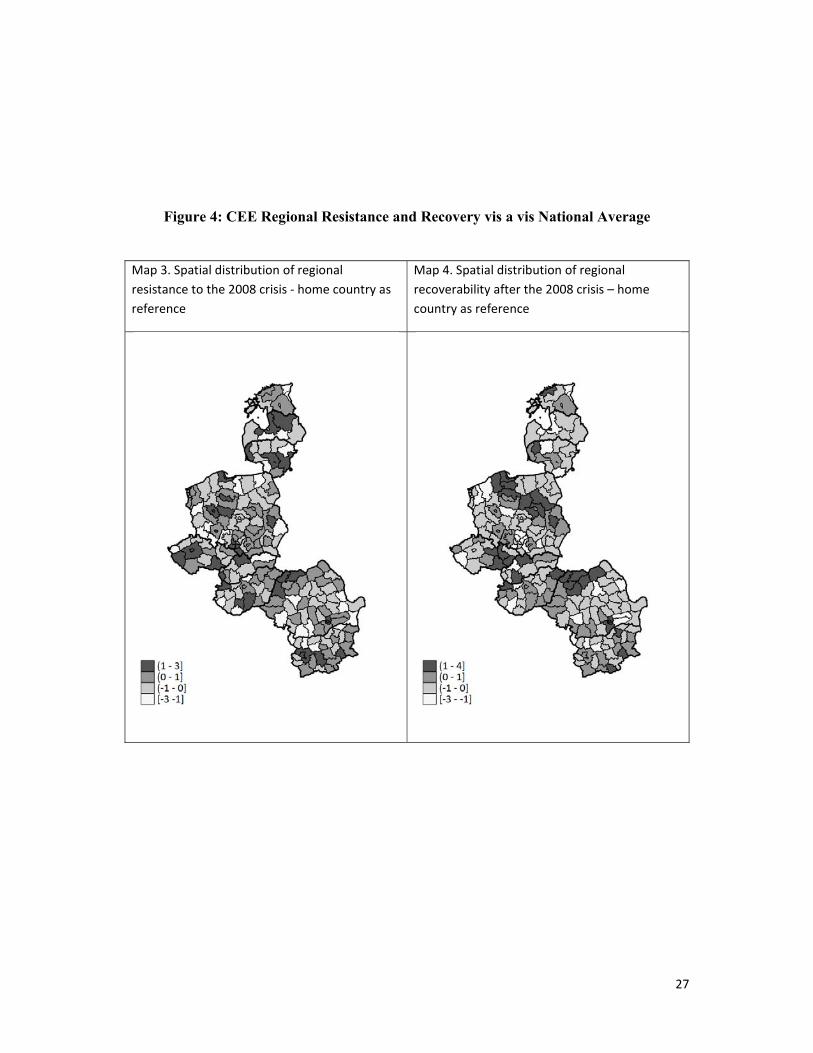
In Figure 4, Maps 3 and 4 illustrate regional resistance and recoverability in the regions

under investigation, taking individual countries as a counterfactual. In this way, the country-

wide layer is removed, and we can focus on region-specific factors only. Once the national

effects are controlled for, there seems to be a rather limited degree of spatial clustering with

regard to resistance and more of it with regard to recoverability. Moreover, regions that did not

lose much employment during the crisis (or even gained employment), such as some capital

cities, often did not recover as much as some other regions.

In order to formally check the existence of spatial dependence or clustering, we

introduce spatial weighting matrices (𝑾) of two forms. The contiguity matrix contains ones,

𝑾 𝑖, 𝑚 , for contiguous regions i and m and zero otherwise. The inverse distance matrix takes

the form:

𝑾 𝑖, 𝑚 1/𝑑 𝑖, 𝑚 (9)

where 𝑑 𝑖, 𝑚 is the distance between regions i and m. In both cases, we use matrices that allow

for cross-national border regional spillovers as well as those that exclude such a possibility.

Clearly, the possibility of spillovers between regions within a country is to be expected. Firms

and workers can move from one region to a neighboring region with relative ease. Movements

between regions in two different countries, even if they are contiguous, may be more difficult.

The 𝑾 matrices enable us to investigate spatial autocorrelation and they are also necessary

for spatial regression effects, should the former be detected.

We test for the existence of spatial autocorrelation by using Moran’s-I test, which

employs the I statistic:

15  

𝐼∑ ∑ , ̅ ̅

∑ ̅ (10)

where N is the number of regions (indexed by i and m) and x is the variable of interest. The

null hypothesis is that the data are randomly distributed across regions. We report the p-values

for the Moran’s I spatial autocorrelation statistic in Table 1. Only in one case, that of the

resilience measure when the inverse distance matrix is assumed, is the null hypothesis of no

spatial autocorrelation not rejected. Residuals are therefore considered to be correlated with

nearby residuals, as defined by 𝑾, meaning that the dependent and explanatory variables

exhibit regional clustering.

V. Explanatory variables

In line with previous studies, we consider explanatory variables that capture regional

productivity differences and differences among regional social and economic structures.

Productivity is measured by gross value added (GVA) per worker. Regional economic

structures are proxied by shares of employment in agriculture and in industry, as well as by

the Krugman specialization index (ksi):

𝑘𝑠𝑖 ∑ (11)

where 𝑧 = j-sector output in region i 𝑍 = total output in region i 𝑣 j-sector output in the reference national economy 𝑉: total output in the reference national economy Low values of the Krugman index indicate that a region’s economic structure closely

resembles the national structure. This might be important, because a policy response to the

crisis can be formulated to reflect the national structure of industry. Regions that exhibit

pronounced differences from the national structure of industrial activity may thus find that

national policies do not address their specific issues effectively.

As for recoverability, we want to check whether, in line with the hypothesis formulated

16  

by Martin and Sunley (2015), regional economies that adapt their structure in response to the

shock so as to maintain core sectors are able to recover more effectively. We do this by means

of the modified Lilien indices (mli) of structural change between two points in time (t0 and t1)

as an explanatory variable in our recoverability equations (Lilien, 1982; Mussida and Pastore,

2012). The index is defined as:

𝑚𝑙𝑖 ∑ 𝑏 ln𝑏

𝑏 ln 𝐵

𝐵 (12)

where

𝑏 = variable of interest (employment or value added) in region i, sector j, time t1

𝐵 = total employment or value added in region i, time t1

𝑏 = average share of sector j in total regional employment or value added (in region

i) in the period between t0 and t1.

The index is a measure of temporal dispersion. It takes the value of zero if no structural changes

occurred between t0 and t1, while higher values are associated with larger structural shifts. The

advantage of this index, as opposed to the original Lilien index, for example, is that it enables

the structural change between two periods to be independent of the time sequence and it

accounts for the weight (size) of the sectors.

Summary statistics for the dependent and explanatory variables are reported in Table 1.

All variables exhibit appreciable variability over the 199 NUTS 3 regions. The resilience

variable , which by construction has a mean of zero, is larger (in absolute value) for the

minimum than for the maximum. That suggests that most severe falls in regional employment,

relative to the national average, were quite large when compared to the margin by which better-

performing regions experienced employment declines relative to the national average. In terms

17  

of recoverability, the opposite is the case; regions that performed better than the national

average appeared to do so by a wider margin that did those regions that underperformed. This

suggest that the resiliency of the CEE regions came at the expense of a widening gap between

well-performing and poorly performing regions. Looking at the Lilien indices, the mean of the

index of structural change in GVA is greater than that of employment. Thus, in the downturn,

the structure of regional output changed more than did the structure of regional employment.

VI. Specification of the Model

Regional resistance and recoverability are modelled within the framework of the more

general SDM model and two models with coefficient restrictions, the spatial autoregressive

model (SAR) and the spatial lag of X (SLX) model. The SDM model is:

𝒚 𝛼𝐢 𝜌𝑾𝒚 𝑿𝛽 𝜺  (13) 

𝜀 ∼ 𝑁 0, 𝜎 𝐼 ) 

where 𝒚 is the n × 1 vector of observations of the dependent variable, 𝐢 denotes a n×1 vector of

ones associated with the intercept term α, ρ is a scalar spatial autoregressive coefficient, 𝑾𝒚 is

the n × 1 vector of the spatially lagged dependent variable, where the proximities are specified

according to a n × n non-stochastic spatial weight matrix 𝑾 and 𝑿 is the n × p matrix including

p explanatory variables.

Equation (13) can be rewritten as:

𝒚 𝑰 𝜌𝑾 𝛼𝐢 𝑰 𝜌𝑾 𝑿𝜷 𝑰 𝜌𝑾 𝜺 (14)

This transformation makes it straightforward to calculate partial derivatives of expected

values of 𝒚 with respect to the explanatory variables as:

, … , 𝑰 𝜌𝑾 𝛽 (15)

Diagonal elements of Equation 15 represent direct effects and off-diagonal effects represent

spillover effects. SAR models enable the estimation of global spatial spillovers, which means

that a change in X in any region is transmitted to all other regions, even when the two regions

18  

are not directly connected (Vega and Elhorst, 2013). Global spillovers include feedback effects

that arise as a result of impacts passing through neighboring regions and returning to the region

from which the change originated.

An alternative approach to modelling spillovers is embedded in the SLX model:

𝒚 𝛼𝐢 𝑿𝛽 𝑾𝑿𝜃 𝜺 (16)

This model produces local spillovers, i.e., those that occur between regions connected to each

other (according to W) and do not contain feedback effects (Golgher and Voss, 2016). In our

study we examine both types of relationships to observe the nature of spatial spillovers.

In the presence of spatial autocorrelation among both dependent and independent

variables, OLS, as well as 2SLS, is inconsistent and needs to be replaced by a better-suited

estimation method (Kelejian and Prucha, 2002). Hence, the models are estimated using

maximum-likelihood estimation corrected for heteroskedasticity, which is both consistent and

relatively efficient compared to its popular alternatives such as spatial two-stage least squares.

We also follow LeSage and Pace (2009) and LeSage and Dominguez (2012), who show

that the coefficients of some spatial models (e.g. the SAR model) cannot be interpreted as if

they were simple partial derivatives, which is also evident in Equation 14. In line with their

arguments, we calculate direct and indirect (spillover) effects, rather than reporting point

estimates. Golgher and Voss (2016) show that the direct impacts in the SAR model can be

computed as 𝑡𝑟 𝑆 𝑾 , where 𝑆 𝑾 is a partial derivative matrix for variable k. Total

impacts are equal to 𝒊 𝑆 𝑾 𝒊 , and indirect impacts are the difference between total and

direct impacts. Locality of spillovers in the SLX model implies that the interpretation of

coefficients is straightforward: direct effects are represented by 𝛽, while indirect effects are

represented by 𝜃.

VII. Estimation results

VII.1 Estimates of the SDM model

19  

Table 2 contains estimation results for the resistance equations. We find a very strong

direct impact of pre-crisis labor productivity before the crisis on regional resilience once the

crisis has struck. In the best-fitted models (judging by pseudo-R2), we also find significant

impact of productivity in neighboring regions on a region’s resistance in those specifications

where we use the inverse of the distance between regions as the distance measure. Thus,

clustering, both positive and negative, is evident in the resistance case and spillover effects are

important. The contiguity matrices do not give evidence of spillovers. This may be because

NUTS-3 regions are sufficiently small so that spillovers from non-contiguous regions can

easily take place. Introducing or restricting cross-border spillovers does not change the results.

The regions with economic structures that differ significantly from the national average

relatively weathered the crisis relatively poorly. This might be because national policy

responses were targeting aggregate national variables, so dissimilar regions could have faced

“policy neglect” during the crisis.

Table 4 presents estimation results of the recoverability equations. Here, we want to

check whether more resistant regions recover more efficiently and, whether structural changes

undertaken during, and possibly in response to, the crisis matter for the recoverability. The

results confirm this hypothesis in two ways. First, the direct effects of resistance and of

structural change, whether in terms of value added or employment have significant effects on

recoverability. Thus regions that fared relatively well in the downturn also tended to have better

recoveries, again emphasizing the disparities between well-performing and poorly-performing

regions. Recoverability also has strong positive spillover effects.5 The direct effect of structural

change is more difficult to interpret. This is because it is not clear whether these changes in

structure were the result of better policies for adaptation to the crisis implemented by certain

                                                            5 Thus, regions recover more efficiently when they are surrounded by other fast-recovering regions, but the neighborhood does not matter for resistance. Why this should be so requires further research.

20  

regions, or whether high-productivity regions are by the nature of their higher-productivity

sectors and (presumably) higher-skilled workers more adaptable in times of crisis.

VII.2 Robustness tests

In line with the discussion in Section II.2, we also estimated the SAR and SLX models.

The parameter estimates (not reported here but available from the authors) for these two models

are very similar to those of the more general SDM model, although the statistical properties of

the two parameter-restricted models are somewhat better. We also experimented with

additional explanatory variables, but the addition of too many variables exhausted the degrees

of freedom quickly.

VIII. Conclusions

In this paper we have examined resiliency, the ability to absorb a and recover from

economic shocks in 199 Nuts-3 regions in CEE following the 2009 global financial crisis. We

find that regional productivity has a clear influence on the ability to resist and recover from

shocks. More productive regions fare better than do regions with low output per worker.

Moreover, regions that resist shocks well also recover to a greater extent. Finally, we find

strong positive regional spillovers, which means that regions tend to form clusters of high-

performing and low-performing areas, a process that exacerbates regional income disparities.

The paper also suggests areas of research on resiliency that deserve further study. The

first is the need to add more covariates to the regressions explaining resistance and recovery.

The second is to include “softer” covariates that reflect social mores and behaviors that may

influence the extent to which the residents of regions are willing and able to respond to shocks

in a flexible way.

21  

References

Acemoglu, D., Robinson, S., and Robinson, J.A., (2002). Reversal of fortune: geography and institutions in the making of the modern world income distribution. Quarterly Journal of Economics, 117, 1231-1294 Laurence Ball (2014) Long-term damage from the Great Recession in OECD countries, European Journal of Economics and Economic Policies: Intervention. Volume 11, Issue 2 pp. 149-160. Baltagi, B. H. And Rokicki, B. (2014). The spatial Polish wage curve with gender effects: Evidence from the Polish Labor Survey. Regional Science and Urban Economics, 49, 36-47. Betti, Gianni, Ruzhdie Bici, Laura Neri, Thomas Pave Sohnesen & Ledia Thomo (2018) Local Poverty and Inequality in Albania, Eastern European Economics, 56:3, 223-245, DOI: 10.1080/00128775.2018.1443015 Christopherson, S., Michie, J., Tyler, P. (2010). Regional resilience: theoretical and empirical perspectives. Cambridge Journal of Regions, Economy and Society, 2010, 3, 3-10. Doran, J. and Fingleton, B. (2018). U.S. Metropolitan area resiliency: Insights from dynamic spatial panel estimation. Environment and Planning A; Economy and Space, 50(1), 111-132. Elshort, J.P. (2009). Spatial panel data model. In: Fischer, M.M., Getis, A. (Eds.), Handbook of Applied Spatial Analysis, Springer, Berlin. Elhorst, J.P., Blien, U., Wolf, K. (2007). New evidence on the wage curve: a spatial panel approach. International Regional Science Review, 30 (2), 173-191 Elhorst, J.P. and Vega, S.H. (2013). On spatial econometric models, spillover effects, and W, ERSA paper. Fingleton, B., Garretsen, H., and Martin, R. (2012). Recessionary shocks and regional unemployment: evidence on the resilience of U.K. regions. Journal of Regional Science 52, 109-133. Golgher, A.B. and Voss P.R. (2016). How to interpret the coefficients of spatial models: spillovers, direct and indirect effects. Spatial Demography 4: 175-205. Haltmaier, Jane (2012) Do Recessions Affect Potential Output? Board of Governors of the Federal Reserve System, International Finance Discussion Paper Number 1066. Hassink, R. (2010). Regional resiliency: a promising concept to explain differences in regional economic adaptability. Cambridge Journal of Regions, Economy and Society, 2010, 3, 45-58. Hudson, R. (2010). Resilient regions in an uncertain world: wishful thinking or practical reality? Cambridge Journal of Regions, Economy and Society, 2010, 3, 11-25.

22  

Kelejian, H.H. and Prucha, I. (2002). 2SLS and OLS in a spatial autoregressive model with equal spatial weights. Regional Science and Urban Economics 32(6): 691-705. Konstantin A. Kholodilin, Aleksey Oshchepkov & Boriss Siliverstovs (2012) The Russian Regional Convergence Process, Eastern European Economics, 50:3, 5-26, DOI: 10.2753/EEE0012-8775500301 LeSage, J.P. and Dominguez M. (2012). The importance of modeling spatial spillovers in public choice analysis. Public Choice 150: 525-545. LeSage, J., and Fischer, M. (2008). Spatial growth regressions: model specification estimation and interpretation. Spatial Economic Analysis, 3, 275-304. LeSage, J.P. and Pace R.K. (2009). Introduction to spatial econometrics. Boca Raton: Taylor & Francis Group. Lilien, D. M. (1982). Sectoral shifts and cyclical unemployment. Journal of Political Economy 90:777-793. Robert F. Martin, Teyanna Munyan, and Beth Anne Wilson (2014), Potential Output and Recessions: Are We Fooling Ourselves? Board of Governors of the Federal Reserve System, IFDP Note, November 12, 2014. https://www.federalreserve.gov/econresdata/notes/ifdp-notes/2014/potential-output-and-recessions-are-we-fooling-ourselves-20141112.html Martin R. L. (2012). Regional economic resilience, hysteresis and recessionary shocks. Journal of Economic Geography 12:1–32. Martin R, Sunley P, Gardiner B and Tyler P. (2016). How regions react to recessions: resilience and the role of economic structure. Regional Studies 50: 561-585 Mussida, C., and Pastore F. (2012). Is there a southern-sclerosis? Worker reallocation and regional unemployment in Italy. Discussion Paper No. 6954, Institute for the Study of Labor (IZA). Pendall, R., Foster, K.A., and Cowell, M. (2010). Resilience and regions: Building understanding of the metaphor. Cambridge Journal of Regions, Economy and Society, 2010, 3, 71-84. Pike, A., Dawley, S., Tomaney, J. (2010). Resilience, adaptation and adaptability. Piketty, T. (2014). Capital in the twenty-first century. Cambridge University Press, London. O'Connor, S., Doyle, E., and Doran, J. (2018). Diversity, employment growth and spatial spillovers amongst Irish regions. Regional Science and Urban Economics, 68, 260-67. Reinhart, Carmen M. and Kenneth S. Rogoff (2014) Recovery from Financial Crises: Evidence from 100 Episodes. NBER Working Paper No. 19823. Simmie, J., and Martin, R. (2010). The economic resilience of region: towards an evolutionary approach. Cambridge Journal of Regions, Economy and Society, 2010, 3, 27-43.

23  

Stiglitz, J.E. (2012), The price of inequality. W.W. Norton & Company, New York. Wolfe, D. A., (2010). The strategic management of core cities: path dependence and economic adjustment in resilient regions. Cambridge Journal of Regions, Economy and Society, 2010, 3, 139-152.

24  

Figure 1: Resilience and Early Recovery of Major Economies

 

 

 

Source: Martin et al. 2014 Source: Martin et al. 2014

 

 

 

 

 

 

25  

 

Figure 2: Resistance and Recovery in the European Union

 

 

 

 

 

 

 

 

 

 

 

0

20

40

60

80

100

120

140

2004 2005 2006 2007 2008 2009 2010 2011 2012 2013 2014 2015

Per capita GDP (const US$) EU‐15 = 100 

Old EU Projected Old EU Actual

New EU Projected New EU Actual

Old EU minus Crisis

26  

 

 

 

Figure 3: CEE Regional Resistance and Recovery vis a vis CEE Average

 

 

 

 

 

 

       

Map 1. Regional resistance – CEE as a counterfactual 

Map 2. Regional recoverability – CEE as a counterfactual 

27  

       

Figure 4: CEE Regional Resistance and Recovery vis a vis National Average   

  

Map 3. Spatial distribution of regional 

resistance to the 2008 crisis ‐ home country as 

reference 

Map 4. Spatial distribution of regional 

recoverability after the 2008 crisis – home 

country as reference 

   

28  

Table 1. Descriptive statistics      

Moran's I (p‐val) 

Variable  Obs      Mean      S.D.      Min  Max  Contiguity matrix  Inverse distance matrix 

     cross‐border     

spillovers 

no cross‐

border 

spillovers 

cross‐border 

spillovers 

no cross‐border 

spillovers 

Resilience  199        0.000           1.008     ‐     3.191            2.140                    0.001            0.009            0.087            0.109     

Recoverability  199  ‐     0.020          0.997     ‐     2.078          3.896                  0.000          0.000          0.000          0.000    

Productivity, 2007  199        0.906           0.176           0.537            1.543                    0.000            0.001            0.000            0.000     

Specialization index, 2007  199        0.233           0.108           0.043            0.685                    0.012            0.004            0.002            0.000     

Employment share in 

agriculture, 2007 

199        0.186          0.143          0.002          0.629                  0.000          0.000          0.000          0.000    

Employment share in 

industry, 2007 

199        0.255           0.076           0.085            0.446                    0.000            0.000            0.000            0.000     

Lilien index of GVA structural change between  2008 and 2010  

199        1.433           0.921           0.171            4.126                    0.000            0.000            0.000            0.000     

Lilien index of employment 

structural change between 

2008 and 2010 

199        1.146           0.588           0.355            3.318                    0.000            0.000            0.000            0.000     

 

 

29  

Table 2. Maximum likelihood estimation results – resistance (SDM Model)  (1)  (2)  (3)  (4)  (5)  (6)  (7)  (8)  (9)  (10)  (11)  (12) 

direct effects    

Productivity 2.221*** 2.210*** 2.126*** 2.077*** 1.993*** 1.982*** 1.734*** 1.699*** 2.232*** 2.233*** 2.036*** 2.002***

[4.98] [4.97] [4.83] [4.66] [5.05] [5.08] [4.39] [4.21] [5.38] [5.45] [4.96] [4.79]

Employment share in agriculture

0.773 0.706 1.168* 1.122

[1.08] [0.99] [1.65] [1.58]

Employment share in industry

-1.443 -1.622 -1.730* -1.670*

[-1.46] [-1.64] [-1.80] [-1.73]

Specialization index -1.251* -1.259* -1.356* -1.331*

[-1.78] [-1.80] [-1.95] [-1.91]

indirect effects

Productivity 0.047 0.146 0.918** 0.461** 0.174 0.268 0.925** 0.465** 0.108 0.19 0.840** 0.416*

[0.22] [0.76] [2.42] [2.11] [0.79] [1.37] [2.44] [2.13] [0.51] [1.01] [2.27] [1.95]

total effects

Productivity 2.268*** 2.356*** 3.044*** 2.537*** 2.167*** 2.250*** 2.659*** 2.164*** 2.340*** 2.423*** 2.877*** 2.418***

[4.49] [4.90] [5.47] [5.45] [4.51] [5.03] [5.50] [5.41] [4.72] [5.21] [5.72] [5.74]

Employment share in agriculture

0.773 0.706 1.168* 1.122

[1.08] [0.99] [1.65] [1.58]

-1.443 -1.622 -1.730* -1.670*

30  

Employment share in industry

[-1.46] [-1.64] [-1.80] [-1.73]

Specialization index

-1.251* -1.259* -1.356* -1.331*

[-1.78] [-1.80] [-1.95] [-1.91]

Intercept -1.993*** -2.033*** -2.323*** -1.930*** -1.446** -1.438** -1.465** -1.100* -1.621*** -1.663*** -1.738*** -1.397**

[-3.31] [-3.43] [-3.89] [-3.32] [-2.37] [-2.39] [-2.47] [-1.82] [-2.84] [-2.97] [-3.18] [-2.56]

W*productivity 0.0569 0.202 2.678** 2.994** 0.21 0.372 2.700** 3.023** 0.13 0.264 2.452** 2.702*

[0.22] [0.76] [2.42] [2.13] [0.79] [1.37] [2.44] [1.95] [0.51] [1.01] [2.27] [1.95]

type of W contig contig inv dist inv dist contig contig inv dist inv dist contig contig inv dist inv dist

cross-border spillovers yes no yes no yes no yes no yes no yes no

country effects yes yes yes yes yes yes yes yes yes yes yes yes

N  199 199 199 199 199 199 199 199 199 199 199 199

Pseudo R2  0.119 0.121 0.144 0.138 0.123 0.129 0.146 0.14 0.128 0.131 0.148 0.143

t‐statistics in brackets *p<0.10, **p<0.05, ***p<0.01 

 

 

 

 

 

 

31  

Table 3. Maximum likelihood estimation results – recoverability (SDM Model)

 (1)  (2)  (3)  (4)  (5)  (6)  (7)  (8) 

direct effects

resistance 0.176*** 0.177*** 0.206*** 0.207*** 0.186*** 0.187*** 0.217*** 0.217*** [2.64] [2.68] [3.06] [3.10] [2.77] [2.81] [3.28] [3.31]

lilien - GVA 0.334** 0.321** 0.377** 0.372**

[2.05] [1.99] [2.30] [2.27]

lilien - employment 0.290* 0.290* 0.317** 0.304** [1.92] [1.94] [2.12] [2.05]

indirect effects

resistance 0.096* 0.107** 0.567 0.211 0.105** 0.118** -0.395 -0.075 [1.93] [2.00] [0.90] [1.11] [1.99] [2.07] [-1.40] [-0.47]

lilien - GVA 0.182* 0.195* 1.037 0.377

[1.68] [1.70] [0.88] [1.08] lilien - employment 0.164 0.184 -0.577 -0.105

[1.58] [1.63] [-1.24] [-0.46] total effects resistance 0.272** 0.284*** 0.773 0.418* 0.292*** 0.306*** -0.178 0.143

[2.55] [2.57] [1.17] [1.85] [2.67] [2.68] [-0.67] [0.84] lilien - GVA 0.516** 0.516** 1.415 0.749*

[2.02] [1.96] [1.13] [1.67] lilien - employment 0.454* 0.474* -0.259 0.199

[1.88] [1.89] [-0.65] [0.81] intercept -0.249* -0.232 -2.29 -0.199 -0.310* -0.300* -0.235 -0.191

[-1.66] [-1.57] [-1.48] [-1.29] [-1.74] [-1.72] [-1.30] [-1.05] W*recoverability 0.428*** 0.438*** 0.518*** 0.530*** 1.992*** 3.807*** 2.472*** 4.272***

[4.10] [4.23] [4.83] [4.99] [4.04] [6.49] [4.07] [6.90] type of W contiguity contiguity inv dist inv dist contiguity contiguity inv dist inv dist cross-border spillovers yes no yes no yes no yes no country effects yes yes yes yes yes yes yes yes N 199 199 199 199 199 199 199 199 Pseudo R2 0.0823 0.0835 0.0607 0.049 0.0725 0.0719 0.0671 0.112

t-statistics in brackets *p<0.10, **p<0.05, ***p<0.01