A quick review of business cycle facts

Chapter 3

Natural logarithm of per capita real GNP: Trend and actual

In general, we can talk about peaks and troughs:

A trough is a relatively large negative deviationfrom trend

A peak is a relatively large positive deviationfrom trend

The amplitude of the business cycle is themaximum deviation from trend

The frequency of the business cycle is the number of peaks in RGDP that occur per year

Is this somehow connected to recessions?A series of positivedeviations from trendin RGDP culminatingin a peak representa boom

A series of negativedeviations from trendin RGDP culminatingin a trough representa recession

Business cycles are persistent!

When RGDP is abovetrend, it tends to stayabove trend

When RGDP is belowtrend, it tends to staybelow trend

But other than what’s previously been said, we cannot say more!

The time series of deviations from trendin RGDP is choppy

There is no regularity in the amplitude

There is no regularityin the frequency

So, is there any hope of anticipating business cycles?

While short-termforecasting is relatively easy(with luck!) …

… long-termforecasting is nearlyimpossible!

This is why we say that business cyclesare unpredictable!

Macroeconomic variables often fluctuate together in patterns that exhibitstrong regularities. These patterns are known as comovements.

To identify comovements we often rely in observation of the variables’ graphs.Generally, graphs of macroeconomic variables come in two different flavors:

1. Time series graphs.

2. Scatter plot graphs.

An example of a time-series graph is the following, comparing GNP and GDP!

GNP and GDP in real terms, 1947-2002

0

2,000

4,000

6,000

8,000

10,000

12,000

1947

1950

1953

1956

1959

1962

1965

1968

1971

1974

1977

1980

1983

1986

1989

1992

1995

1998

2001

Bill

ions

of 2

000

dolla

rs

GNP GDP

The variables moveacross time.

You always see how time is evolving in the X-axis!

The Y-axis has the values for the variable(s)!

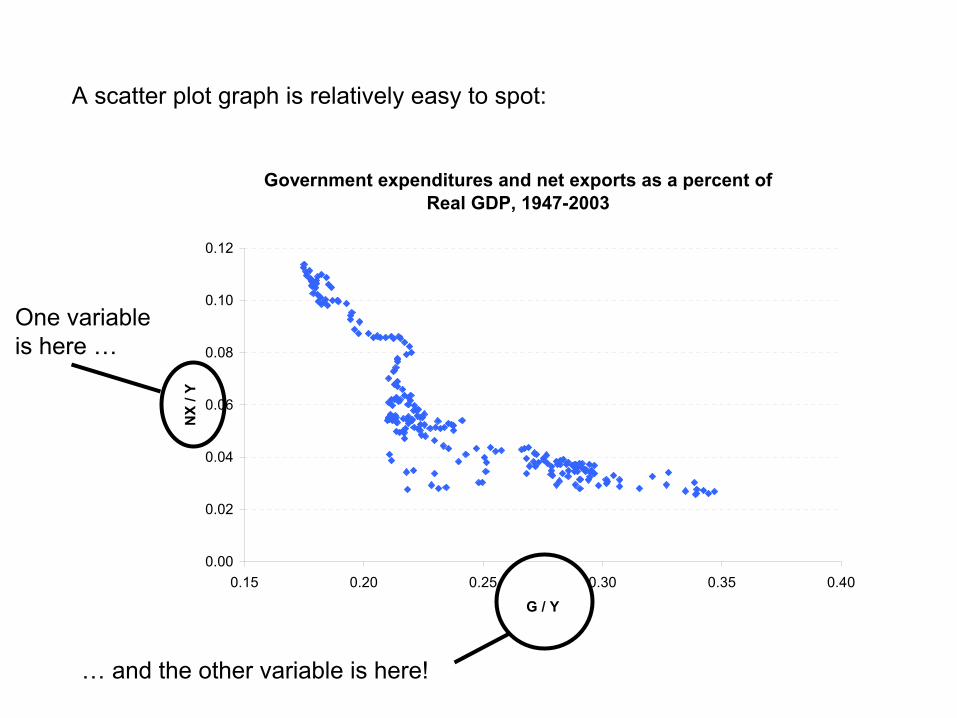
A scatter plot graph is relatively easy to spot:

Government expenditures and net exports as a percent of Real GDP, 1947-2003

0.00

0.02

0.04

0.06

0.08

0.10

0.12

0.15 0.20 0.25 0.30 0.35 0.40

G / Y

NX

/ Y

… and the other variable is here!

One variableis here …

Note that this is not a scatter plot graph!

GDP in real terms, 1947-2002

0

2,000

4,000

6,000

8,000

10,000

12,00019

47

1950

1953

1956

1959

1962

1965

1968

1971

1974

1977

1980

1983

1986

1989

1992

1995

1998

2001

Bill

ions

of 2

000

dolla

rs

GDP

We have time (years) here!

When looking at graphs, we want to distinguish between series that exhibitpositive or negative correlation! In a time series graph

For a scatter plot graph, it’s even easier!

We are mostly interested in how individual economic variables comove with GDP.

1. An economic variable is procyclical if its deviations from trend are positivelycorrelated with deviations from trend in RGDP.

2. Negatively correlated deviations generate a countercyclical variable.

3. Variables which are neither procyclical nor countercyclical are called acyclical.

More definitions:

2. If RGDP helps in predicting the future path of the variable, it is a laggingvariable.

3. Variables which neither lead nor lag RGDP are called coincident variables.

1. If a macro variable helps in predicting the future path of RGDP, we say thatIt is a leading variable.

Finally, we are interested in the volatility of the macroeconomic variables.

A measure of cyclical variability is the standard deviation of the percentagedeviations from trend.

Imports are morevolatile than RGDP!

If we are to construct a macroeconomic model which helps us understand business cycles and the economy, it’d better be the case that it is able toreplicate the regularities and comovements that we observe in RGDP andits components!

Else, it just doesn’t work.

Hence, let’s take a look at Consumption and GDP:

Cyclicality?Procyclical

Lead / lag?Coincident

Volatility to GDP?Smaller

Investment and GDP:

Cyclicality?Procyclical

Lead / lag?Coincident

Volatility to GDP?Larger

Prices (the implicit GDP price deflator) and GDP:

Cyclicality?Countercyclical

Lead / lag?Coincident

Volatility to GDP?Smaller

Money supply and GDP:

Cyclicality?Procyclical

Lead / lag?Leading

Volatility to GDP?Smaller

Employment and GDP:

Cyclicality?Procyclical

Lead / lag?Lagging

Volatility to GDP?Smaller

Average labor productivity and GDP:

Cyclicality?Procyclical

Lead / lag?Coincident

Volatility to GDP?Smaller

Summing up! This is what our model should replicate!