A Quasi-Likelihood Approach to Zero-Inflated Spatial Count ... · A Quasi-Likelihood Approach to...

POUR L'OBTENTION DU GRADE DE DOCTEUR ÈS SCIENCES

acceptée sur proposition du jury:

Prof. M. Troyanov, président du juryProf. S. Morgenthaler, directeur de thèse

Prof. V. Panaretos, rapporteur Prof. Y. Tillé, rapporteur

Prof. M.-P. Victoria-Feser, rapporteur

A Quasi-Likelihood Approach to Zero-Inflated Spatial Count Data

THÈSE NO 5442 (2012)

ÉCOLE POLYTECHNIQUE FÉDÉRALE DE LAUSANNE

PRÉSENTÉE LE 23 jUILLET 2012

À LA FACULTÉ DES SCIENCES DE BASECHAIRE DE STATISTIQUE APPLIQUÉE

PROGRAMME DOCTORAL EN MATHÉMATIQUES

Suisse2012

PAR

Anthea MONOD

The most important thing you can do,

is do a lot of work.

— Ira Glass

To my grandfather,

Thomas Thường Doãn Trần

AcknowledgmentsGoing all the way through school is no easy quest, and as with many things in life, doesn’t

always go the way one plans: having started my doctoral studies at the University of Neuchâtel,

I now find myself finishing at EPFL. I am very lucky to have had the help and support of

numerous people on my academic venture, without which the completion of this thesis would

not have been possible.

I am deeply indebted and profoundly grateful to my advisor Professor Stephan Morgenthaler

for his trust, confidence and support. His patience, insight and steady encouragement ren-

dered each conversation a valuable learning opportunity, motivating me throughout my

doctoral studies. I wish to express my deepest gratitude for his generosity and his reassuring

presence on all matters, be it related to research or pertaining to my career path. I am particu-

larly thankful for his guidance and advice as I applied for the next step of my academic career,

which resulted in a postdoctoral fellowship at the Technion Israel Institute of Technology for

the fall of 2012.

I would like to thank the members of my jury, Professor Victor Panaretos, Professor Yves Tillé

and Professor Maria-Pia Victoria-Feser for their time in reading and discussing my work, and

for their helpful comments and feedback. I would also like to thank Professor Marc Troyanov

for having presided the jury.

I owe very special thanks to Achim Nonnenmacher for so kindly and tirelessly answering my

endless questions, and not just the ones about MATLAB. Thanks also go to Kjell Konis for

helpful discussions on programming.

I would like to express thanks to Professor Yanyuan Ma, my first advisor at the University of

Neuchâtel who is now at Texas A&M University, for giving me the opportunity to start a Ph.D.

Though we were not able to see the project through together, I am grateful to her for having

left me in good hands, and thank her for her continued support. I am also very grateful to

my former colleagues at the University of Neuchâtel, especially Professor Yves Tillé, for their

support and understanding during my transition to EPFL.

I thank Soazig L’Helgouac’h and Corine Diacon from the University of Neuchâtel, and Anne-

Lise Courvoisier, Nadia Kaiser and Léonard Gross from EPFL, for their cheerful presence,

v

Acknowledgments

efficiency, and ever willingness to help with administrative and technical matters. I also thank

EPFL, the University of Neuchâtel and the Swiss National Science Foundation for financial

support of my doctoral studies.

Last but not least, I am grateful to my family and my friends: those here in Switzerland, for

making these years fondly memorable, as well as those scattered all over the world, who never

let distance stop them from encouraging me.

A. M.

Geneva, July 2012

vi

AbstractThe increased accessibility of data that are geographically referenced and correlated increases

the demand for techniques of spatial data analysis. The subset of such data comprised of

discrete counts exhibit particular difficulties and the challenges further increase when a large

proportion (typically 50% or more) of the counts are zero-valued. Such scenarios arise in many

applications in numerous fields of research and it is often desirable to infer on subtleties of

the process, despite the lack of substantive information obscuring the underlying stochastic

mechanism generating the data. An ecological example provides the impetus for the research

in this thesis: when observations for a species are recorded over a spatial region, and many

of the counts are zero-valued, are the abundant zeros due to bad luck, or are aspects of the

region making it unsuitable for the survival of the species?

In the framework of generalized linear models, we first develop a zero-inflated Poisson gener-

alized linear regression model, which explains the variability of the responses given a set of

measured covariates, and additionally allows for the distinction of two kinds of zeros: sampling

(“bad luck” zeros), and structural (zeros that provide insight into the data-generating process).

We then adapt this model to the spatial setting by incorporating dependence within the model

via a general, leniently-defined quasi-likelihood strategy, which provides consistent, efficient

and asymptotically normal estimators, even under erroneous assumptions of the covariance

structure. In addition to this advantage of robustness to dependence misspecification, our

quasi-likelihood model overcomes the need for the complete specification of a probability

model, thus rendering it very general and relevant to many settings.

To complement the developed regression model, we further propose methods for the simula-

tion of zero-inflated spatial stochastic processes. This is done by deconstructing the entire

process into a mixed, marked spatial point process: we augment existing algorithms for the

simulation of spatial marked point processes to comprise a stochastic mechanism to generate

zero-abundant marks (counts) at each location. We propose several such mechanisms, and

consider interaction and dependence processes for random locations as well as over a lattice.

Keywords: Generalized linear models (GLM), Generalized estimating equations (GEE), Zero-

inflated Poisson (ZIP) models, Spatial analysis, Marked point processes.

AMS Subject Classification: 60G55, 62J12, 62M3, 82B20, 92D40.

vii

RésuméLa disponibilité croissante des données géographiquement référencées et corrélées augmente

par conséquent l’exigence de techniques d’analyse des données spatiales. Le sous-ensemble

de telles données comprenant les décomptes discrets présentent des difficultés particulières

et les défis ne font qu’augmenter quand il y a une grande proportion (typiquement de plus de

50%) des décomptes qui prennent la valeur zéro. De tels scénarios se présentent en plusieurs

applications dans des nombreux champs de recherche, là où il est en plus désirable d’en

déduire des complexités du processus. Néanmoins, le manque d’information substantifique

obscurcit le processus stochastique implicite qui génère les données. Un exemple écologique

nous fournit la motivation de la recherche de cette thèse : quand les observations d’une espèce

sont notées sur une région spatiale, et la majorité de celles-ci prennent la valeur zéro, les

zéros sont-ils dûs à la malchance, ou indiquent-ils des aspects de la région qui la rendent

inadéquate à la survie de l’espèce ?

Dans le cadre des modèles linéaires généralisés (GLM), dans un premier pas, nous dévelep-

pons un modèle linéaire généralisé de Poisson modifié en zéro, qui explique la variabilité des

réponses étant donné un ensemble de covariables mesurées, et explique en outre la distinction

des deux types des zéros : ceux qui sont dûs à l’échantillonnage (ceux dûs à la « malchance »)

et ceux qui sont dûs à la structure (ceux qui fournissent de l’intuition sur le processus qui

génère les données). Nous adaptons ensuite ce modèle au cadre spatial, en incorporant de

la dépendance dans le modèle au moyen d’une stratégie de quasi-vraisemblance générale

et flexible qui fournit des estimateurs consistants, efficaces et asymptotiquement normaux,

même sous des hypothèses de covariance éronnées. En sus de cet avantage de robustesse à

la malspecification du modèle, notre modèle de quasi-vraisemblance évite le besoin d’une

spécification complète d’un modèle de probabilité, ce qui le rend très général et pertinent à

des nombreuses applications.

En complément au modèle de régression mentionné ci-dessus, nous proposons de plus des

méthodes pour la simulation d’un processus stochastique spatial modifié en zéro. Ceci est fait

en décomposant le processus entier en un processus ponctuel spatial qui est en outre marqué

et mélangé : nous augmentons les algorithmes de simulation des processus ponctuels spatiaux

marqués existants pour inclure un mécanisme stochastique qui détermine si les marques

des locations qui prennent la valeur zéro sont dûs à l’échantillonnage ou s’ils sont dûs à la

structure. Nous considérons la simulation sur un réseau ainsi qu’en des locations aléatoires.

ix

Résumé

Mots-clés : Modèles linéaires généralisés (GLM), équations d’estimation généralisées (GEE),

modèles de Poisson modifiés en zéro (ZIP), analyse spatiale, processus ponctuels marqués.

x

RiassuntoLa crescente disponibilità di dati geolocalizzati e spazialmente correlati fa aumentare l’esi-

genza di tecniche di analisi di dati spaziali. In tale ambito, i dati che comprendono conteggi

discreti presentano particolari difficoltà: da un punto di vista matematico, il calcolo integrale

e differenziale vi hanno un’utilità limitata, mentre, da un punto di vista statistico, manca una

base che fornisca per i dati non-gaussiani lo stesso livello di precisione di quelli continui. Le

sfide non fanno che aumentare quando una proporzione grande (tipicamente oltre il 50%) di

conteggi nulli. Simili scenari si presentano in diverse applicazioni ed in numerosi campi della

ricerca ed è spesso necessario fare inferenze sui dettagli di un certo fenomeno nonostante la

mancanza di informazioni sostanziali sul processo stocastico che soggiace alla generazione

dei dati in esame. Un esempio in Ecologia fornisce la motivazione della ricerca di questa tesi:

quando le osservazioni di una specie sono raccolte in una regione spaziale, e la maggioranza

delle occorrenze sono nulle, gli zeri sono dati dalla “sfortuna” o indicano aspetti della regione

che la rendono inadeguata alla sopravvivenza della specie?

Nel quadro dei modelli lineari generalizzati (GLM), in un primo passo sviluppiamo un modello

di regressione lineare generalizzata di Poisson con inflazione di zeri, che spiega la variabilità

delle risposte dato un insieme di predittori misurati, e che permette di distinguere due tipi

di zeri: quelli dovuti al campionamento (alla “sfortuna”) e quelli strutturali (che fornisco-

no un’intuizione sul processo generatore dei dati). In un secondo passo, adattiamo questo

modello alla configurazione spaziale incorporandovi dipendenze attraverso una tecnica di

quasi-verosimiglianza generale e flessibile, che fornisce stimatori consistenti, efficienti ed asin-

toticamente normali, anche in presenza di ipotesi di covarianza erronee. Oltre a questo van-

taggio di robustezza contro la malspecificazione, il nostro modello di quasi-verosimiglianza

supera il bisogno di specificazione completa di un modello di probabilità, cosa che lo rende

molto generale e adatto a numerose applicazioni.

In complemento al modello di regressione summenzionato, proponiamo inoltre un algoritmo

per la simulazione di un tale processo stocastico spaziale. Questo contributo è raggiunto fra-

zionando l’intero processo in un processo puntuale con interazioni, spaziale, misto, marcato e

tripartito: un primo meccanismo stocastico guida l’ubicazione aleatoria dove le osservazioni

sono registrate, mentre un secondo genera in ogni locazione le realizzazioni discrete (i conteg-

gi), molti dei quali prendono valore nullo. Il terzo componente stocastico determina se gli zeri

sono quelli di campionamento, o se sono dati dalla struttura del processo senza inflazione di

xi

Riassunto

zeri. Estendendo gli algoritmi di simulazione esistenti con l’inclusione di un meccanismo di

generazione di zeri, il metodo proposto permette di generare processi puntuali di Poisson che

sono inflazionati di zeri e correlati spazialmente.

Parole chiave: Modelli lineari generalizzati (GLM), equazioni di stima generalizzata (GEE),

modelli di Poisson inflazionati di zeri (ZIP), analisi spaziale, processi puntuali marcati.

xii

ContentsAcknowledgments v

Abstract/Résumé/Riassunto vii

Notation xvi

Introduction 1

1 Spatial Data 7

1.1 Point-Referenced Data . . . . . . . . . . . . . . . . . . . . . . . . . . . . . . . . . . 8

1.1.1 Stationarity . . . . . . . . . . . . . . . . . . . . . . . . . . . . . . . . . . . . 9

1.1.2 Spatial Covariance . . . . . . . . . . . . . . . . . . . . . . . . . . . . . . . . 10

1.1.3 Isotropy . . . . . . . . . . . . . . . . . . . . . . . . . . . . . . . . . . . . . . 12

1.1.4 Variogram Fitting and Exploratory Data Analysis . . . . . . . . . . . . . . 26

1.1.5 Kriging . . . . . . . . . . . . . . . . . . . . . . . . . . . . . . . . . . . . . . . 28

1.2 Areal Unit Data . . . . . . . . . . . . . . . . . . . . . . . . . . . . . . . . . . . . . . 31

1.2.1 Measures of Spatial Association . . . . . . . . . . . . . . . . . . . . . . . . 31

1.2.2 Local and Global Modeling . . . . . . . . . . . . . . . . . . . . . . . . . . . 32

1.3 Point Pattern Data . . . . . . . . . . . . . . . . . . . . . . . . . . . . . . . . . . . . 40

1.3.1 Poisson Processes . . . . . . . . . . . . . . . . . . . . . . . . . . . . . . . . . 40

1.3.2 The Palm Distribution and the Papangelou Intensity . . . . . . . . . . . . 43

1.3.3 Descriptive Statistics for Complete Spatial Randomness . . . . . . . . . . 45

1.3.4 Estimating the Intensity . . . . . . . . . . . . . . . . . . . . . . . . . . . . . 47

1.3.5 Modeling Point Processes . . . . . . . . . . . . . . . . . . . . . . . . . . . . 50

2 Discrete Data and Zero-Inflation 55

2.1 Discrete Distributions . . . . . . . . . . . . . . . . . . . . . . . . . . . . . . . . . . 56

2.1.1 The Binomial Distribution . . . . . . . . . . . . . . . . . . . . . . . . . . . 56

2.1.2 The Poisson Distribution . . . . . . . . . . . . . . . . . . . . . . . . . . . . 57

2.1.3 The Negative Binomial Distribution . . . . . . . . . . . . . . . . . . . . . . 58

2.2 Overdispersion . . . . . . . . . . . . . . . . . . . . . . . . . . . . . . . . . . . . . . 59

2.2.1 Zero-Inflation . . . . . . . . . . . . . . . . . . . . . . . . . . . . . . . . . . . 61

2.3 Existing Models: A Review . . . . . . . . . . . . . . . . . . . . . . . . . . . . . . . . 63

2.3.1 Models for Zero-Inflated Data . . . . . . . . . . . . . . . . . . . . . . . . . 63

xiii

Contents

2.3.2 The Zero-Inflated Poisson (ZIP) Model . . . . . . . . . . . . . . . . . . . . 64

2.3.3 Models for Correlated Zero-Inflated Data . . . . . . . . . . . . . . . . . . . 65

2.3.4 The Zero-Inflated Generalized Additive Model (ZIGAM) . . . . . . . . . . 67

2.3.5 Other Approaches to Zero-Inflated Data . . . . . . . . . . . . . . . . . . . 69

2.3.6 Models for Zero-Inflated Spatial Data . . . . . . . . . . . . . . . . . . . . . 71

3 A Generalized Linear Model for Zero-Inflated Spatial Count Data 75

3.1 The Generalized Linear Model (GLM) . . . . . . . . . . . . . . . . . . . . . . . . . 75

3.1.1 Exponential Families . . . . . . . . . . . . . . . . . . . . . . . . . . . . . . . 76

3.1.2 Maximum Likelihood Estimation and Inference . . . . . . . . . . . . . . . 77

3.1.3 Generalized Linear Models for Spatial Data . . . . . . . . . . . . . . . . . . 78

3.2 M-Estimation: Marginal Models and

Quasi-Likelihood Estimation . . . . . . . . . . . . . . . . . . . . . . . . . . . . . . 79

3.3 The Two-Component Approach . . . . . . . . . . . . . . . . . . . . . . . . . . . . 81

3.4 A Zero-Inflated Poisson Generalized Linear Model . . . . . . . . . . . . . . . . . 83

3.4.1 Log-Likelihood and Score Equations . . . . . . . . . . . . . . . . . . . . . 84

3.4.2 Asymptotic Behavior . . . . . . . . . . . . . . . . . . . . . . . . . . . . . . . 86

3.5 Introducing Spatial Dependence:

Generalized Estimating Equations (GEEs) . . . . . . . . . . . . . . . . . . . . . . 89

3.5.1 Generalized Estimating Equations

for the Spatial Zero-Inflated Poisson Model . . . . . . . . . . . . . . . . . 90

3.5.2 Asymptotic Behavior . . . . . . . . . . . . . . . . . . . . . . . . . . . . . . . 92

4 Simulation Studies 95

4.1 On the Concavity of the Log-Likelihood Function . . . . . . . . . . . . . . . . . . 96

4.2 Simulation Design: Parameter Settings and Data Generation . . . . . . . . . . . 96

4.3 The Independent Case . . . . . . . . . . . . . . . . . . . . . . . . . . . . . . . . . . 97

4.3.1 Computing the Empirical Semivariogram . . . . . . . . . . . . . . . . . . 100

4.4 The Spatially-Correlated Case: The Matérn Correlogram . . . . . . . . . . . . . . 102

4.5 Example: Counts of Noisy Friarbirds . . . . . . . . . . . . . . . . . . . . . . . . . . 105

5 Generating Point Processes for Zero-Inflated Spatial Data 109

5.1 Marked Point Processes . . . . . . . . . . . . . . . . . . . . . . . . . . . . . . . . . 110

5.1.1 Marking Models . . . . . . . . . . . . . . . . . . . . . . . . . . . . . . . . . . 110

5.1.2 Motion Invariance . . . . . . . . . . . . . . . . . . . . . . . . . . . . . . . . 112

5.1.3 First-Order Characteristics . . . . . . . . . . . . . . . . . . . . . . . . . . . 113

5.1.4 The Palm Distribution Revisited . . . . . . . . . . . . . . . . . . . . . . . . 114

5.1.5 Second-Order Characteristics . . . . . . . . . . . . . . . . . . . . . . . . . . 115

5.1.6 Other Complexities of Spatial Point Processes: Interaction Models . . . . 117

5.2 Simulating Spatial Point Processes . . . . . . . . . . . . . . . . . . . . . . . . . . . 118

5.2.1 Metropolis-Hastings Algorithms . . . . . . . . . . . . . . . . . . . . . . . . 118

5.2.2 Simulation Based on Spatial Birth and Death Processes . . . . . . . . . . 122

5.2.3 Perfect Simulation . . . . . . . . . . . . . . . . . . . . . . . . . . . . . . . . 125

xiv

Contents

5.3 Generating Zero-Inflated Point Processes . . . . . . . . . . . . . . . . . . . . . . . 129

5.3.1 Zero-Inflated Lattice Counts . . . . . . . . . . . . . . . . . . . . . . . . . . 129

5.3.2 Zero-Inflated Counts for Marked Poisson Processes . . . . . . . . . . . . . 133

Conclusion 138

A Complete Derivation of the Fisher Information 143

Bibliography 150

Curriculum Vitæ 175

xv

NotationAbbreviationsAR Autoregressive

CAR Conditionally autoregressive

CFTP Coupling from the past (algorithm)

COZIGAM Constrained zero-inflated generalized additive model

EM Expectation-maximization (algorithm)

GAM Generalized additive model

GEE Generalized estimating equation

GLM Generalized linear model

i.i.d. Independent and identically distributed

GLMM Generalized linear mixed model

MCMC Markov chain Monte Carlo

MLE Maximum likelihood estimate

Prob Probability

SRS Stochastic recursive sequence

Var Variance

Vol Volume

ZIGAM Zero-inflated generalized additive model

ZIP Zero-inflated Poisson

xvii

Notation

Sets, Functions and OperatorsThe mathematical symbols for the classification of numbers will be depicted by boldfaced

letters using the facility \mathbf, included in the add-on AMS Fonts package (amsfonts).

While the facility \mathbb exists in the same package to produce the typeface style that is

often seen in printed text, for instance in the notation for the real numbers as R, the use

of blackboard bold in print is incorrect as the double struck bold characters are meant as a

substitute for boldface typing when writing by hand. See discussions given by Jean-Pierre

Serre (2010) [Ser], and online at [com] and [MAT], for the use of boldfaced letters versus the

blackboard bold typeface.

[a,b[ Left-closed, right-open, proper and bounded interval from a to b,

x ∈ R : a ≤ x < b

(a,b) Ordered pair

R Real numbers, ]−∞,+∞[

Z Integers, ]−ℵ0, . . . ,−1,0,1, . . . ,+ℵ0[

R+ Nonnegative real numbers, [0,+∞[

Z+ Nonnegative integers, [0,1,2, . . . ,+ℵ0[

N Natural numbers, [1,2, . . . ,+ℵ0[

Rd d-dimensional Euclidean space

C∞ Class of smooth (infinitely differentiable) functions

∂s Neighborhood (disc) of the point s

∂i Set of neighbors of the cell i

b1 Unit ball in Rd

b(x,r ) Ball centered at the point x with radius r

dn(x) Nearest-neighbor distance, distance from the point x to its nearest neighbor

1(E) Indicator function, 1(E) =1 if the event E is true,

0 otherwise.

exp(·) Exponential function, exp(x) = ex

log(·) Natural logarithm, log(x) = ln(x) = loge (x)

logit(·) Logistic function, logit(x) = 1

1+e−x

Γ(·) Gamma function, Γ(u) =∫ +∞

0e−t t u−1d t

xviii

Notation

Kν(·) Modified Bessel function of the second kind of order ν, canonical solution to the

Bessel differential equation x2 d y2

d x2 +xd y

d x+ (x2 −ν2)y = 0 with a purely imaginary

argument, Kν(x) =∫ +∞

0exp(−x cosh t )cosh(νt )d t

‖x‖ Euclidean norm of the vector x, ‖x‖ =√

x21 +x2

2 +·· ·x2n

⟨x,y⟩ Inner product of the vectors x and y, ⟨x,y⟩ =∑ni=1 xi yi

f (·) Fourier transform of the function f (·)ˆf (·) Conjugate Fourier transform of the function f (·)

g−1(·) Link function, page 75

v(·) Variance function, page 76

Vµ Diagonal matrix with entries given by values of the variance function v(·), page 78

k(·) Kernel function, page 15

K (·) Ripley’s K function, page 46

Mathematical Symbols\ Set exclusion

Ac Complement of the set A

∼A Reflexive relation on the set A

|x| Absolute value of the scalar x

|B | Area of the region B

µL(A) Lebesgue measure of a Lebesgue-measurable set A

n(x) Nearest point to x

na(x) Number of points within a distance a of the point x

N (A) Cardinality of the set A

I(n×n) Identity matrix of dimension n ×n

X > Transpose of the matrix X

X ∗ Adjoint (conjugate transpose) of the matrix X , X ∗ = X >

f ′(·) First-order derivative of the function f (·)f ′′(·) Second-order derivative of the function f (·)(n

k

)Binomial coefficient,

(n

k

)= n!

k !(n −k)!,0 ≤ k ≤ n

xix

Notation

Random Variables and Probabilistic OperatorsZ (·) Spatial random variable Z : D ⊆ Rd → R

E [X ] Expectation of the random variable X

E [X |Y ] Conditional expectation of the random variable X given the random variable Y

Var(X ) Variance of the random variable X

Cov(X ,Y ) Covariance of the random variables X and Y

Σ Covariance matrix

`(·) Log-likelihood function

Sβ Score function with respect to the parameter vector β

SQuasiβ

Quasi-score function with respect to the parameter vector β, page 80

I (β) Fisher information with respect to the parameter vector β

d−→n→∞ Convergence in distribution

d= Equality in distribution

Probability Distributions∼ Distribution symbol of a random variable

fZ (·) Probability density function or probability mass function of the random

variable Z

N (µ,σ2) Normal distribution with mean µ and variance σ2

χ2(k) Chi-squared distribution with k degrees of freedom

Exp(ε) Exponential distribution with parameter ε

Γ(k,ϑ) Gamma distribution with shape parameter k and scale parameter ϑ

P (λ) Poisson distribution with parameter λ

PTruncated(λ,n0) Truncated Poisson distribution with parameter λ and truncation point n0

Unif([0,1]

)Uniform distribution on the interval [0,1]

UnifSkew([0,1]

)Skewed uniform distribution on the interval [0,1]

ZIP(α,λ) Zero-inflated Poisson distribution with mixing probability α and Poisson

parameter λ

xx

Notation

Notation Pertaining to Spatial AnalysisD Index set of spatial coordinates, s = (s1, s2, . . . , sd )>; D ⊆ Rd , page 7

M Mark space, page 110

Ω State space of a spatial point process,Ω=⋃∞i=0

x ∈D : N (x) = i

, page 125

ΩD Finite configuration space, set of all realizations of a random variable z(s) ∈Ω for

all s ∈D , finite point configurations x ⊂D : |x| < +∞, page 33, 119

S Natural state space of a Markov chain, y ∈ΩD : gY (y) > 0, where gY (·) is the target

distribution, page 124

γ(·) Semivariogram, page 13

C (·, ·) Covariogram, spatial covariance function, page 10

r (·, ·) Correlogram, spatial correlation function, page 10

R(ϑ) Correlation matrix with entries given by some correlogram r (·, ·), page 78

bZ (z, ·) Spatial birth probability density function on D , page 122

dZ (z, ·) Spatial death probability mass function on D , page 122

xxi

Introduction

With the recent phenomena of globalization and the rapid advancement of technology comes

the accessibility of new kinds of data revealing complex structures, and in turn the demand for

methods to analyze and interpret them. Such is the case with data that are geographically ref-

erenced and correlated, which inspired a new demand for analysis and modeling techniques,

forming the field of statistics that is now known as spatial analysis. Though the theoretical

foundations stem from geophysical and environmental applications, there is no doubt regard-

ing the breadth of the scope and relevance of such techniques, especially when considering

that spatial variation may occur on the micro- as well as the macroscale. In situations where

measurements are collected, analyzed and interpreted, often the data take the form of counts,

and when objects or occurrences are counted, there is also the possibility that there are none

to count. All of these characteristics are inherent to the scenario that provides the back-drop

to the work of this thesis.

This scenario arises in a multitude of fields and applications, from engineering, such as in

operations research, information technology; to applied sciences, for example in quality

control, medicine, astrophysics, economics, sociology, psychology, epidemiology; to pure

sciences, such as biology, chemistry and physics. Our motivating question that provides the

impetus for the work in this thesis pertains to an application of ecology: when observations

for a species are recorded over a spatial region, and many of the counts are zero-valued, are

the abundant zeros due to bad luck, or are aspects of the region making it unsuitable for the

survival of the species?

Methods for discrete data have been developed over the years as statistical methods have

been developed, and while spatial analysis is a comparatively new field, interest has been so

rampant that canonical results and a comprehensive methodology are already well established.

Data sets comprising abundant zeros have also been studied and methods for them developed

for nearly as long as spatial data, the situation for which proves to be no less challenging than

that for spatial or discrete data. When there are so many zero counts in a data set (say 50% or

more), it is tempting to ignore them and perform analysis purely on the observable counts,

or to treat them as outliers or missing data. While such approaches have been concurrently

developed in other fields of statistics, that is, methods to handle outliers and missing data,

writing zeros off as such may have highly significant effects on the conclusions drawn from

such analysis techniques: the zeros, in fact, may provide important and extremely informative

1

Introduction

insight into the underlying process.

When the underlying stochastic process generating the few counts that are actually observed

is obscured by so many zeros, extracting information on the process becomes difficult. While

methods have been, and are continuously being, developed to handle zero-inflated counts,

there are important subtleties to consider that affect the specific strategies that handle zero-

inflated data. One such nuance arises when we seek interpretation of the zeros as well as

the counts. In such a scenario, simply separating the zeros from the counts and modeling

each component independently is not conducive to achieving the goal, not if our objective is,

for instance, to explain the occurence or detect the stimulus for the dispersion of a certain

species over a spatial region. With such an aim, the distinction between the zeros is important

because it may signify whether there is an underlying biological stimulus inherent in the

region as to why the species cannot survive, or whether the sampling techniques used so far

are inadequate, which are two very different sources of zeros that have very different impacts

on the conclusion drawn. This distinction has been picked up on in the past by researchers

seeking to answer precisely this kind of question, but, to the best of our knowledge, not in a

spatial context from a frequentist perspective using generalized linear models. Moreover, from

the spatial analytic point of view, and again to the best of our knowledge, the investigation on

how such zero-inflated counts arise has not has not been initiated. The work in this research

strives to address both of these issues, since knowing how something originates is key to

explaining why things are the way they are, which provides a sound basis for the development

of methods to deal with them.

Main Research Contributions

The type of data that we tackle in this thesis is marked spatial point processes, where the marks

associated at each point of the spatial stochastic process represent the random species count

at that location (point). In particular, we are interested in cases when these counts exhibit a

large proportion of zeros of 50% or more; the size of the zero proportion is also considered to

be random. We approach this scenario from two points of view: modeling and simulation.

From the modeling perspective, we propose our first research contribution in the form of

a regression model for the variability of the count observations from a set of measured co-

variates. The main challenges associated with modeling zero-inflated spatial count data

are the abundant zeros of the responses, particularly distinguishing between sampling and

structural zeros; the discrete nature of count data, for which the same well-established and

precise methods for handling Gaussian data are not applicable; and the spatial orientation

and correlation of the recorded observations. Our approaches to each of these challenges

draw in ideas from other domains and are tied together by developments that are grounded in

the flexible, encompassing, and general theory of M-estimation.

To address the excessive zeros and the problem of differentiating between the two zero types,

we develop a zero-inflated Poisson generalized linear model, building on existing results that

2

Introduction

have been previously established to handle count data with abundant zeros. The randomness

of the counts and their excessive zeros is modeled by a zero-inflated version of the classical

Poisson distribution, which is often assumed for counts. The Poisson distribution also allows

zero observations, which explains the structural zeros, those inherent to the process; the

zero-inflation component provides for sampling zeros, those due to human or measurement

error. Constructing our model in the framework of generalized linear models allows these com-

ponents to be combined and modeled based on given covariate information, and moreover,

simultaneously addresses the discrete nature of our data.

The estimation of our generalized linear model parameters are derived from maximum likeli-

hood estimation, which is a special case of M-estimation, which also provides the unifying

framework of the theory we implement to incorporate spatial dependence. Marginal models

provide the flexibility that allows the inclusion of covariance matrices amongst generalized

estimating equations, an idea that borrows from the theory of quasi-likelihood, which is also a

special case of M-estimation; in specifying a spatial covariance matrix to incorporate, which

either may be estimated from the data or postulated from theory, we allow for spatial depen-

dence to be included in the model. Moreover, implementing the theory of quasi-likelihood

returns consistent and efficient estimators, even under misspecification of the dependence

structure, and without the requirement of a complete probability specification.

As a result, spatially-correlated, zero-inflated count data can be modeled from given covariate

information, and the types of zeros that contribute to so many null responses can be differenti-

ated. Spatial effects can also be included, even though they are generally difficult to determine

precisely, which may also aggravate the intractability of a complete probability model. With

our quasi-likelihood model, neither task is necessary, yet the distinction between structural

and sampling zeros, and the consistency, efficiency and asymptotic normality of estimators

are not compromised.

From the simulation perspective, we aim to grasp the mechanics of how such data is generated

to propose our second research contribution. Doing this involves decomposing the entire

process to consider each source of randomness individually. At the base of the process is the

spatial nature of the data, that generates points (locations) in space in a random manner, which

entails the study of spatial point processes. Imposed on these points is the random process

that generates the counts observed at each of these points, which augments the study of

spatial point processes to that of marked point processes. Marked point processes are complex

statistical structures, not only due to the randomness of two stochastic processes coupled

together which already presents considerable issues in terms of the number of parameters

and the definition of moment structures, but also because there may be correlation within

the the mark-point couple, as well as correlation between other mark-point couples in space,

which only further complicates the issues of parameters and moment structures. The large

proportion of zeros contributes a third stochastic component to the marked point process.

In studying mechanisms that generate point processes and their adaptations to marked point

3

Introduction

processes, we further augment the mark distribution to a zero-inflated setting. In doing

so, we propose two algorithms for the simulation of spatially-correlated zero-inflated count

processes: one for points on a lattice, and one for zero-inflated multitype marked point

processes exhibiting pairwise interaction. We also propose several stochastic mechanisms

for the generation and inclusion of abundant zeros, which may be applied to either point

configuration.

The aim of constructing such algorithms for generating data of such kind is towards the spec-

ification of clearly defined probabilities. Defining specific probabilities for such processes

was the difficulty that inspired the previous approaches in the literature, such as that of the

inclusion of random effects, the use of marginal models, and even our own quasi-likelihood

approach, as means to avoid specifying a complete probability model. With clearly defined

probabilities, the classical approach of full maximum likelihood becomes possible; our pro-

posed algorithms provide a first step in this direction.

Outline

This thesis is organized as follows: Chapter 1 provides the preliminaries on spatial data in the

form of an overview; we define and outline important aspects of each of the three types of

spatial data: point-referenced data, areal unit data, and point pattern data. In particular, we

provide complete specifications of focal points of spatial analysis, including a full construction

of the celebrated Matérn class of isotropic correlograms by Fourier inversion and complete

derivation the algorithm of kriging, which is the spatial analog of classical linear least squares

estimation algorithms. We also provide the technical generation of Markov random fields

via the specification of a Gibbs potential, and derive thinning and clustering constructions

for spatial point processes. Chapter 2 narrows in on the type of spatial data of the setting

of this thesis, namely discrete, correlated, spatially-varying data exhibiting abundant zero

responses, which corresponds to point pattern data. We provide definitions and constructions

of canonical discrete probability distributions, and detail the technical challenges faced in our

spatial data scenario. We then review the literature on existing approaches to these difficulties,

and on applications where this scenario arises and where existing techniques have been

implemented.

Chapter 3 begins with a characterization of the unifying theory of generalized linear models

for the analysis of non-Gaussian, clustered, correlated, longitudinal, and spatial data. It is

in this framework that we construct the first research contribution of this thesis: a Poisson

generalized linear model for spatial zero-inflated count data, and corresponding generalized

estimating equations that allow for the incorporation of spatial dependence. Chapter 4

provides the results of series of simulations and numerical experiments performed to test the

finite sample performance of the model in a general setting under various data scenarios.

Chapter 5 revisits point pattern spatial data and reviews existing algorithms for simulation of

spatial point processes. We delve into further detail on the case of marked point processes,

4

Introduction

where now covariate information and responses may be associated with the points (locations),

to provide the theoretical framework for the second research contribution of this thesis:

algorithms for the generation of zero-inflated Poisson marked processes on a lattice, and in

space.

This thesis concludes with a discussion on the methods developed, and proposals for future

research projects based on and stemming from this work.

5

1 Spatial Data

Data that are geographically referenced and perhaps temporally correlated arise in many

fields of research. Examples include climatology, which may require techniques to analyze a

meteorological study of temperature and precipitation data taken on a network of monitoring

stations with a mean surface that reflects elevation and perhaps a trend in location; epidemiol-

ogy, where the interest may lie in the analysis of public health data, such as occurrences of an

infectious disease by county and/or year, given patient data such as family history and lifestyle

information; and finance and marketing, which may be real estate marketing to predict sales

of single family homes with demographic information on potential home buyers such as

age, income bracket, level of education, as well as information on the house such as area,

size, and other characteristics. In encountering such data, we are interested in statistical

inference: modeling of trends and correlation structures; estimation of underlying model

parameters; hypothesis testing or model comparison; and prediction at unobserved locations

or time points. Though the aims are very familiar and what has inspired statistics as soon as

any form of information was collated and there was a need for analysis and interpretation,

spatial statistics in particular inspires the need for new techniques. While longitudinal (panel)

data appears to be similar in nature, the added subtlety presented in spatial analysis is the

establishment of a coordinate system, or a means of referencing points in relation to one

another in space.

Spatial stochastic processes are collections of random variables Z (·) indexed by the set D ⊆ Rd ,

which contains spatial coordinates s = (s1, s2, . . . , sd )>Z (s) : s ∈D

or

Z (s,ω) : s ∈D ,ω ∈Ω

,

to make randomness explicit, where (Ω,F ,P ) is a probability space composed of the sample

spaceΩ, σ-algebra F , and probability assignment P .

In many practical applications of spatial statistics, stochastic processes vary in the plane

with d = 2; the coordinates are given by the ordered pair s = (x, y)> (longitude and lattitude).

Spatio-temporal stochastic processes are indexed by a set on a space-time manifold with

7

Chapter 1. Spatial Data

d = 3; the coordinates s = (x, y, t )> comprise a time variable. Stochastic processes where d ≥ 2

are referred to by the general term of random field, which itself generates a vast and general

subject encompassing statistics and probability, and relies heavily on theory drawn from

geometry and topology. Spatial data take the form of realizations z = z(s) of random variables

of spatial stochastic processes, Z : D ⊆ Rd → R, and may belong to one of three types, each

characterized by the set D :

• Point-Referenced Data: Z (·) is observed at the location s ∈ Rd , where s varies continu-

ously over a fixed subset D ⊂ Rd .

• Areal Unit Data: D is a fixed subset partitioned into finitely many areal units with well-

defined boundaries; the units may be regularly shaped, as in the case of lattice or grid

cell partitions, or irregularly shaped, as in the case of counties or postal code areas.

• Point Pattern Data: D is a random subset, its index set provides the location of random

events, which make up the spatial point pattern. Z (·) may be an indicator random

variable, or may provide additional covariate information, which produces a marked

point pattern process.

We now provide an overview of each type of spatial data, detailing important aspects of

each. Exhaustive documentation of each type, comprehensive theoretical foundations, and

in particular what follows in the current chapter may be found in several canonical refer-

ences, including those of Ripley (1981, 1984) [Rip81], [Rip84], Cressie (1993)[Cre93]; Chilès

& Delfiner (1999) [CD99]; Wackernagel (2003) [Wac03]; Banerjee, Carlin & Gelfand (2004)

[BCG]; Schabenberger & Gotway (2005) [SG05]; and The Handbook of Spatial Statistics (2010)

[GDFG10], among others.

1.1 Point-Referenced Data

The basic component of point-referenced data is a spatial process indexed by location,

Z (s) :

s ∈D

where D ⊂ Rd , which is conceptually similar to time series analysis where d = 1.

Referring back to the concept of spatial stochastic processes being random fields with d ≥ 2,

in constructing the theoretical basis for dealing with such data, it is important to note that the

issue at hand is not the analysis and interpretation of a data set comprised of outcomes of n

experiments conducted, but rather of n observations collected over a spatial region D of a

single experiment conducted. We aim to inference on the make-up of one generated random

field, and not on the existence of several realizations (although more generally speaking, it may

of course also be generated more than once). The above-mentioned epidemiological example

provides an illustration of this concept: the spatial analysis of an infectious disease entails the

occurrences of patients being diagnosed with the disease over a region (we may wish to predict

where the disease may spread next, for instance), and not the disease occurring in the same

region and affecting the same patients multiple times. Indeed, with an effective sample size of

8

1.1. Point-Referenced Data

one, the task of inferencing (or doing statistics with just one observed realization) proves to

be challenging. However, as noted by Whittle (1954) [Whi54], imposing certain conditions on

the stochastic properties of the random field provides a starting point towards modeling and

prediction.

1.1.1 Stationarity

Let us assume that

Z (s) : s ∈ D

has mean µ(s) = E[

Z (s)]

and that the variance of Z (s),

Var(Z (s)

), exists for all s ∈ D ⊆ Rd . This set-up provides a basis for the introduction of the

concept of stationarity, which essentially reduces the task of dealing with absolute coordinates

in the index set D to considering only translations between points in D .

Definition 1.1.1. The random field

Z (s) : s ∈ D

is said to be strongly stationary if for any

n ≥ 1, any set of n sites s1,s2, . . . ,sn and any h ∈ Rd , the distribution of the collection of random

variables

Z (s1), Z (s2), . . . , Z (sn)

is identical to that of

Z (s1 +h), Z (s2 +h), . . . , Z (sn +h); i.e.

Prob(Z (s1) ≤ z1, · · · , Z (sn) ≤ zn

)= Prob(Z (s1 +h) ≤ z1, · · · , Z (sn +h) ≤ zn

).

In other words, the spatial distribution of the random field is invariant under translation of

members of its index set (coordinates): a strictly stationarity random field repeats over its

region of definition, and the observation of Z (s) does not allow one to draw inferences about

s.

The specification of strong stationarity implies the existence of other types of stationarity. In

contrast to strong stationarity which imposes conditions on the entire spatial distribution,

weak stationarity relaxes the rigidity of such demands by imposing conditions only on second

moments of the distribution.

Definition 1.1.2. The random field

Z (s) : s ∈ D ⊂ Rd

is said to be weakly stationary if

E[

Z (s)]=µ for all s ∈D , and Cov

(Z (s), Z (s+h)

)=C (h) for all h ∈ Rd such that s,s+h ∈D .

In other words, for a weakly stationary random field, the mean is constant and the covariance

relationship between the values of the process at any two locations can be summarized by a

covariogram C (·), which depends only upon the separation (or lag) vector h ∈ Rd . Assuming

weak stationarity immediately implies that the variance of a weakly stationary spatial process

is the same everywhere, since Cov(Z (s), Z (s+0)

)=C (0) = Var(Z (s)

)for all s ∈D .

When all variances are assumed to exist, strong stationarity implies weak stationarity, though

the converse need not be true, since in general, entire probability distributions cannot be

defined only by the first and second moments. An important exception for which the converse

does hold is that of Gaussian processes, since a normal distribution is completely specified

by its mean and covariance (see Adler (1981) [Adl81] and Adler & Taylor (2007) [AT07] for

more details in the context of random fields). The importance of Gaussian processes lies

9


in the consideration of asymptotics, and specifically, in the central limit theorem, where

the long-run result of many experiments is approximately Gaussian (see, for instance, Lind-

gren (1976) [Lin76], Billingsley (1995) [Bil95], Le Cam & Yang (2000) [LCY00], Bartoszynski &

Niewiadomska-Bugaj (2008) [BNB08]).

A yet weaker version of weakly stationarity is that of intrinsic stationarity, which requires

only the existence of the first and second moments of the differences

Z (s+h)−Z (s)

for all

points s ∈D and any separation vector h ∈ Rd . Intrinsic stationarity provides no information

on the joint distribution of

Z (s1), Z (s2), . . . , Z (sn), meaning that likelihoods cannot be con-

structed when the only information given on the stochastic process is intrinsic stationarity.

Again, weak stationarity implies intrinsic stationarity; the converse need not be true. Cressie

(1993) [Cre93] shows that the class of intrinsic stationary processes encompasses the class of

weakly stationary processes.

The antipodal concepts of strict stationarity (being too rigid) and intrinsic stationarity (being

too lax) to proceed in interesting directions for modeling, weak stationarity is often a sufficient

assumption made about the spatial process. Admittedly, this can be unreasonable, with rami-

fications of inaccurate inference and false conclusions drawn when the assumption of weak

stationarity is made about the process, and it is not. Nevertheless, a thorough understanding

of concepts of stationarity is an important prerequisite to studying nonstationarity ([Whi54]).

1.1.2 Spatial Covariance

The covariogram C (·) is a function that dictates the variability of a spatial stochastic process (it

is the spatial covariance function), and as in classical statistics, is of considerable importance

in spatial analysis and modeling.

Definition 1.1.3. A covariogram C (·, ·) is a valid and well-defined spatial covariance function

if and only if it is a positive-definite function; i.e.

n∑i=1

n∑j=1

ai a j C (si −s j ) ≥ 0

for all locations s in a given D and all ai , a j ∈ R. Recall that a function C : R → C is said to be

positive-definite if for any x1, x2, . . . , xn ∈ R, the n ×n matrix A with entries ai j =C (xi −x j ) is

a positive semi-definite matrix; i.e. it is diagonalizable and all its eigenvalues are nonnegative.

Provided that C (0) > 0, the correlogram r (·, ·) is given by r (si −s j ) :=C (si −s j )/C (0).

This definition is intuitive, since the double sum corresponds to the variance of the linear com-

bination of the coefficients a = (a1, a2, . . . , an)> and the n-vector Z = (Z (s1), Z (s2), · · · , Z (sn)

)>,

Var(a>Z).

The acclaimed theorem of Bochner (1932) [Boc32] from the field of harmonic analysis provides

the construction of positive-definite functions; it states that a continuous function is positive-

10


definite if and only if it is the Fourier transform of a finite, nonnegative measure.

Theorem 1.1.4 (Bochner, 1932 [Boc32]). A continuous function C (·) on Rd is positive-definite

if and only if it has the spectral representation

C (h) =∫

Rde i h>xdF (x),

where F (·) is a finite, nonnegative measure on Rd .

The validity of Bochner’s theorem may be intuited via the relation between multiplication and

conjugate products in the Fourier domain, in particular, by considering Fourier transforms of

positive functions f (·). We consider the one-dimensional case for x ∈ R to illustrate the idea

behind the proof. For a function C (·) taking the form

C (x) =∫ +∞

−∞e i xω f (ω)dω,

the conjugate Fourier transform of f (·), denoted by C∗(·), is

C∗(x) = ˆf (ω) =∫ +∞

−∞e i xω f (ω)dω=

∫ +∞

−∞e−i xω f (ω)dω=C (−x).

In matrix notation, we may define a matrix A by C (·) such that the elements of A are given by

ai j :=C (xi −x j ). Then the conjugate of C (·), C∗(·), admits the adjoint (conjugate transpose) of

A, A>, since (A>)i j = (A) j i =C (x j −xi ) =C∗(xi −x j ). In general, a matrix B is positive-definite

if there exists some other matrix D such that B = DD∗, since

⟨Bv,v⟩ = ⟨DD∗v,v⟩ = ⟨D∗v,D∗v⟩ = ‖D∗v‖2 ≥ 0.

By putting A = BB∗, we obtain positive-definiteness, and in particular the function C (·) that

defines the entries of A is the Fourier transform of ϕ(·), where f (·) = |ϕ(·)|2.

The harmonic analytic proof is given in Bochner (1932) [Boc32], Bochner (1955) [Boc55] and

Todorovic (1992) [Tod92]; a probabilistic proof may be found in Bingham & Parthasarathy

(1968) [BP68]. In probability theory, we have by Bochner’s theorem that the function C (·) must

be the characteristic function of a symmetric probability density function. For our purposes,

the function C (·) is the covariogram, and the function f (·) is its corresponding spectral density

(see for instance Sneddon (1995) [Sne95] for further detail on spectral theory and Fourier

transforms).

Under the assumption of weak stationarity, the covariogram implies other important proper-

ties summarized in the following theorem.

Theorem 1.1.5. The covariogram C (·) of a weakly stationary spatial stochastic process possesses

the following properties:

11


(i) C (0) ≥ 0

(ii) C (·) is an even function: C (h) =C (−h)

(iii) C (0) ≥ |C (h)|

(iv) C (h) = Cov(Z (s), Z (s+h)

)= Cov(Z (0), Z (h)

)(v) If Ci (·) are valid covariograms and bi ≥ 0 for all i = 1, . . . ,n, then

∑ni=1 bi Ci (h) is also a

valid covariogram

(vi) If Ci (·) are valid covariograms for i = 1, . . . ,n, then∏n

i=1 Ci (h) is also a valid covariogram

(vii) If C (·) is a valid covariogram in Rd , then it is also a valid covariogram in Rp for p < d

Proof. Properties (i) and (ii) follow from the definition of a classical covariance function; for

Property (ii), we make a change of variables u := s+h, so that C (h) = Cov(s,s+h) = Cov(u−h,u) = Cov(u,u−h) =C (−h). Property (iii) that |C (h)| is finite and in particular smaller than

C (0) is obtained by the Cauchy-Schwarz inequality. Since, as mentioned previously, a weakly

stationary covariogram only depends upon the separation vector h and does not depend on

absolute coordinates of members of D , the spatial process may be translated to the origin to

obtain Property (iv). Properties (v) and (vi) follow as spatial analogs to classical covariance

functions (see for instance Loève (1946) [Loè46]), by the definition of the covariogram given in

Definition 1.1.3. A direct computation given independent random variables Z1 and Z2 shows

that sums of covariances give covariances

Cov(Z1+Z2, Z ′1+Z ′

2) = E[(Z1+Z2)(Z ′

1+Z ′2)

]= E [Z1Z ′1]+E [Z2Z ′

2] = Cov(Z1, Z ′1)+Cov(Z2, Z ′

2),

the case for multiple covariances extending accordingly, and similarly, products of covariances

give covariances

Cov(Z1Z2, Z ′1Z ′

2) = E[(Z1Z2)(Z ′

1Z ′2)

]= E[(Z1Z ′

1)(Z2Z ′2)

]= Cov(Z1Z ′1, Z2Z ′

2).

An argument for Property (vii) is given by Matérn (1986) [Mat86] that covariance functions are

Hermitian and since Rn ⊂ Rn+1, the class of covariance functions on Rn+1 contains the class

of covariance functions on Rn so if C (·) is a valid covariance function on Rn+1, it is also valid

on Rn .

1.1.3 Isotropy

Another stringent assumption, yet interesting in its simplicity and interpretability, which may

be made on random fields of spatial stochastic processes is that of isotropy. To discuss this

concept, we introduce the semivariogram.

12


Definition 1.1.6. The semivariogram is a function γ : Rd → Rd+ defined by

γ(h) := 1

2Var

(Z (s+h)−Z (s)

);

2γ(·) is referred to as the variogram. If, in particular, γ(·) is of univariate argument and depends

only upon ‖h‖ and E[

Z (s+h)−Z (s)]= 0, the spatial stochastic process is said to be isotropic.

Under weak stationary, the semivariogram and covariogram are related by γ(h) =C (0)−C (h)

and as such, it is common to see theory presented using both functions, though statisticians

more commonly use the covariogram and geostatisticians tend to use the semivariogram. Use

of the semivariogram is particularly convenient under the assumption of intrinsic stationary,

by definition, since the expression for a semivariogram only makes sense, and can thus only

be written, under the assumption of at least intrinsic stationarity. One should note, however,

that the functions are not equally well-defined: the semivariogram γ(·) may be determined

from a given covariogram C (·), since by definition,

2γ(h) = Var(Z (s+h)−Z (s)

)= Var(Z (s+h)

)+Var(Z (s)

)−2Cov(Z (s+h), Z (s)

)=C (0)+C (0)−2C (h) = 2

(C (0)−C (h)

),

which implies γ(h) =C (0)−C (h). The converse, however, need not be true: the covariogram

may not necessarily be determined from a semivariogram since it may not be identified; both

the covariogram C (·) and the semivariogram γ(·) depend only upon the separation vector

h, and it is entirely possible for the latter to take the form γ(h) = C (0)−C (h)+ constant,

thus posing a problem of identifiability. However, under the assumption of ergodicity, which

essentially allows expectations over the sample spaceΩ to be estimated by spatial averages (I

see Adler (1981) [Adl81] and Cressie (1993) [Cre93] for further detail), both the covariogram C (·)and the semivariogram γ(·) are well-defined: A sufficient condition for ergodicity (Adler (1981)

[Adl81]) is that

C (h) −→‖h‖→∞

0.

Thus, for an ergodic spatial process, lim‖h‖→∞γ(h) = lim‖h‖→∞C (0)−C (h) =C (0), and via a

change of variables for notational convenience, we have C (h) =C (0)−γ(h) = lim‖u‖→∞γ(u)−γ(h), so C (h) is well-defined as long as lim‖h‖→∞γ(h) exists. Under ergodicity, intrinsic sta-

tionarity also implies weak stationarity.

Definition 1.1.7. Given an isotropic variogram, we may define

• the nugget of the process, γ(0+) = lim‖h‖→0+ γ(‖h‖) = τ2 > 0

• the sill of the process, σ2Z = lim‖h‖→∞γ(‖h‖)

• the range of the process, a = inf

h : γ(‖h‖) = lim‖h‖→∞γ(‖h‖)

, i.e. the lag h beyond

which Z (s) and Z (s+h) are no longer correlated; the effective range a0 is defined by

13


Figure 1.1: The Nugget, Range, and Sill of a Variogram.

a corresponding effective separation h0, the distance that gives the range at which the

correlation decreases to 0.05

These notions are illustrated in Figure 1.1.

The nugget effect thatγ(0+) = τ2 > 0 arises, but cannot happen mathematically for L2-continuous

or mean squared continuous processes; i.e. processes Z (·) for which E[(Z (s+h)−Z (s))2

]→ 0

as h → 0. For

limh→0

E[(Z (s+h)−Z (s))2]= lim

h→02(C (h)−C (0)

),

if C (h) 6→C (0) as h → 0, the random field cannot be mean squared continuous at s. If we expect

continuity of the random field, the only explanation for the nugget effect is measurement

error. To illustrate measurement in the context of modeling, we decompose the process to

comprise an independent mean effect µ(·), an independent spatial random effect ω(·) with

corresponding variance σ2, and an independent pure error effect ε(·) with corresponding

variance τ2,

Z (s) =µ(s)+ω(s)+ε(s).

See Cressie (1993) [Cre93] for further detail on this decomposition. This gives a variance of

Var(Z (s)

)=σ2 +τ2, and for the covariance, we have

Cov(Z (s), Z (s′)

)= Cov(ω(s)+ε(s),ω(s′)+ε(s′)

)=σ2r (s−s′)

and lim(s−s′)→0σ2r (s−s′) =σ2. Note, however, that in the spatial context, unlike in the context

of time series analysis, such a decomposition is not unique. Recall that the Wold decompo-

sition theorem due to Wold (1954) [Wol54] states that there exists a unique decomposition

for any weakly stationary time series into the sum of a purely deterministic and a purely non-

determinstic time series, which are uncorrelated and both weakly stationary (see Hamilton

14


(1994) [Ham94] and Gouriéroux & Monfort (1997) [GM97] for further detail). In the spatial

setting, however, notions of past, present and future are not obvious to define, which limits

the existence of an analagous Wold decomposition theorem for spatial data. In Z2, however, a

notion of the past can be defined by considering half-planes and Wold-type decomposition

theorems have been established for such a space, for instance, by Körezlioglu & Loubatan

(1986) [KL86].

In contrast to isotropy, the concept of anisotropy stipulates that association depends upon the

direction and distance of the separation vector between locations.

Example 1.1.1. Geometric anisotropy generates elliptical contours,

C (s1 −s2) ∝ r((s1 −s2)>A(s1 −s2)

),

for some positive-definite matrix A. Contours of constant association in the case of geometric

anisotropy are elliptical; in particular, the corresponding to r = 0.05 provides the effective

range for each spatial direction.

Example 1.1.2. Geometric product anisotropy extends geometric anisotropy,

C (s1 −s2) ∝ r1((s1 −s2)>A1(s1 −s2)

)r2

((s1 −s2)>A2(s1 −s2)

),

for positive-definite matrices A1, A2.

Geometric and product geometric anisotropy are particular cases of range anisotropy, which

suggests the parallel definitions of sill anisotropy, where given a semivariogramγ(·), limc→∞γ(c·

h/‖h‖) depends on h, implying that the process is not ergodic, and of nugget anisotropy, where

a given semivariogram γ(·), limc→0γ(c ·h/‖h‖) depends on h, implying that no pure error can

be introduced to the mode.

There exists a variety of parametric forms as candidates for isotropic covariograms; we mention

a few here. Other models can be found in Cressie (1993) [Cre93] and Schabenberger & Gotway

(2005) [SG05].

Example 1.1.3. A weakly stationary random field has a representation via the convolution of

a kernel function and white noise random field ([SG05]); the covariogram of such a random

field is itself the convolution of the kernels k(·),

C (h) =σ2∫

uk(u)k(u+h)du,

where σ2 is the white-noise variance. Choosing the indicator function for the sphere in Rd

with diameter 1/ϑ, 1(‖u‖ ≤ 1/(2ϑ)

), as a kernel function (see Chilès & Delfiner (1999) [CD99])

15


generates the spherical class of isotropic covariograms,

C (‖h‖) =

0 if 1/ϑ≤ ‖h‖;

σ2∫ 1

ϑ‖h‖(1−u2)(d−1)/2du if 0 < ‖h‖ ≤ 1/ϑ;

τ2 +σ2 otherwise.

For the case that d = 3, the spherical covariogram and its corresponding semivariogram are

given by

C (‖h‖) =

0 if 1/ϑ≤ ‖h‖;

σ2(1− 3

2ϑ‖h‖+ 12 (ϑ‖h‖)3

)if 0 < ‖h‖ ≤ 1/ϑ;

τ2 +σ2 otherwise.

γ(‖h‖) =

τ2 +σ2 if 1/ϑ≤ ‖h‖;

τ2 +σ2(

32ϑ‖h‖− 1

2 (ϑ‖h‖)3)

if 0 < ‖h‖ ≤ 1/ϑ;

0 otherwise.

The property that the correlation is exactly zero at a separation distance ‖h‖ = 1/ϑ for the

spherical class is, according to Stein (1999) [Ste99], a statistical disadvantage in practical

modeling and applications in its unrealism.

Example 1.1.4. The exponential class of covariograms and corresponding semivariograms are

given by

C (‖h‖) =σ2e−ϑ‖h‖ if ‖h‖ > 0;

τ2 +σ2 otherwise.

γ(‖h‖) =τ2 +σ2

(1−e−ϑ‖h‖) if ‖h‖ > 0;

0 otherwise.

In contrast to the spherical model, for the exponential model, the sill is only reached asymp-

totically, meaning that strictly speaking, the range a = 1/ϑ is infinite and it is for such models

that working with the effective range is meaningful. To find the effective range, note that for

‖h‖ > 0, we have

C (‖h‖) = lim‖u‖→∞

γ(‖u‖)−γ(‖h‖) = τ2 +σ2 −(τ2 +σ2(1−e−ϑ‖h‖))=σ2e−ϑ‖h‖,

however, since γ(0) = τ2, we set C (0) = τ2 +σ2, so

C (‖h‖) =τ2 +σ2 if ‖h‖ = 0,

σ2e−ϑ‖h‖ if ‖h‖ > 0.

With this specification, the correlation between two points at distance ‖h‖ apart is e−ϑ‖h‖;

as expected, we have e−ϑ‖h‖ = 1 for t = 0+ and e−ϑ‖h‖ → 0 when t →∞. For the exponential

model, when e−ϑ‖h0‖ = 0.05, the effective range a0 ≈ 3/ϑ since log(0.05) ≈−3.

16


The exponential model is the equivalent of a time series covariance function of autoregressive

order one AR(1) in continuous time and is used in the modeling of longitudinal data by Jones

(1993) [Jon93] and repeated measures by Schabenberger & Pierce (2002) [SP02] in addition to

spatial data.

Example 1.1.5. When |ν| ≤ 2, the powered exponential class of covariograms and correspond-

ing semivariograms are generated by

C (‖h‖) =σ2e−(ϑ‖h‖)ν if ‖h‖ > 0;

τ2 +σ2 otherwise.

γ(‖h‖) =τ2 +σ2

(1−e−(ϑ‖h‖)ν

)if ‖h‖ > 0;

0 otherwise.

Note that the exponential class is a particular case of the powered exponential class.

The Matérn Class of Isotropic Correlograms

The 1960 doctoral thesis of Matérn [Mat60] (revised in 1986 [Mat86]) provides the general

and versatile so-named Matérn class of everywhere-continuous covariograms for isotropic

spatial processes which has proven to be seminal in modeling in many applications, such as

that of geostatistics, in modeling geothermal field temperatures by Mateu, Porcu, Christakos

& Bevilacqua (2007) [MPCB07], and wind fields by Wikle, Berliner & Milliff (2003) [WBM03],

Fuentes, Chen, Davis & Lackmann (2005) [FCDL05], Xu, Wikle & Fox (2005) [XWF05]; agricul-

ture, in modeling soil data by Minasny & McBratney (2005) [MM05], and Lesch & Corwin (2008)

[LC08] and crop yields by Clifford & Tuesday (2004) [CT04]; physics, in modeling heat diffusion

processes by Kelbert, Lenenka & Ruiz-Medina (2005) [KLRM05] and predicting photometric

redshift by Way, Foster, Gazis & Srivastava (2009) [WFGS09]; epidemiology, in modeling oc-

currence of cancer by Baladandayuthapani, Veerabhadran, Mallick, Hong, Lupton, Turner

& Carroll (2008) [BMH+08]; and urban developmant by Duan, Gelfand & Sirmans (2010)

[DGS10], among others. Moreover, the Matérn class generalizes and encompasses two other

important models commonly used in geostatistical applications, including the exponential

family given above in Example 1.1.4; its form is given in the following definition.

Definition 1.1.8. The Matérn class of isotropic covariograms takes the form

C (‖h‖) = 2σ2

Γ(ν)

(ϑ‖h‖

2

)νKν

(ϑ‖h‖),

whereσ2 denotes the variance of the spatial process; the parameters ϑ and ν pertain to the range

of spatial dependence and the smoothness of the process, respectively; and Kν(·) is the modified

Bessel function of the second kind of order ν. Its corresponding spectral density function takes

the form

f (ω) =σ2 ϑ2ν

Γ(ν)Γ(1

2

) (ϑ2 +ω2)−(ν+ 12 ).

17


The smoothness of a random field is dependent on the fractal dimension (see Adler (1981)

[Adl81]), a local property determined by the asymptotic behavior of the covariogram at an

infinitesimally small separation, whose value depends upon the smoothness parameter ν

for a random field possessing a Matérn covariance structure: the larger the value of ν, the

smoother the process Z (·). Moreover, in two dimensions d = 2, the process is bνc times L2-

differentiable (or mean squared differentiable). In contrast, the strength of spatial depen-

dence is characterized by the range parameter ϑ which decays exponentially with separation.

Together, this enables the Matérn class of covariograms the cover a wide range of behaviors

while maintaining the interpretability of the parameters.

Alternative parameterizations of this class exist in Stein & Handcock (1993) [SH89], Handcock

& Wallis (1994) [HW94] and Stein (1999) [Ste99], and may be used depending on the objective

or application. Alternative parameterizations may give more convenient representations of

corresponding spectral density functions and subclasses of the Matérn class, or to make the

effective range more explicit.

We now build upon the framework given in Matérn (1986) [Mat86] and give the explicit

construction of this class based on Fourier inversion, which makes use of Bochner’s theo-

rem and uses results from the theory of stationary processes; we will construct the class

of correlograms, the correlogram being proportional to the covariogram. The notation

used for the variable in the correlation (time) domain will be x with its norm denoted by

v = ‖x‖ =√

x21 +·· ·+x2

d ; the variable in the spectral (or frequency) domain will be ω with

its norm denoted by w = ‖ω‖ =√ω2

1 +·· ·+ω2d . Other notation in this construction follows

Matérn (1986) [Mat86].

The construction of the Matérn class of isotropic spatial correlations begins by considering

the isotropic correlation function

r1(v) = e−a2v2 ⇐⇒ r1(x) = exp−a2(x2

1 +·· ·+x2d )

.

This is a particular case of the more general form of the characteristic function of the multi-

variate normal distribution

ϕ(ω) = exp−ω>Aω,

whereω>Aω is a non-negative quadratic form. Following a result of Cramér (1940) [Cra40],

characteristic functions for random variables constitute correlation functions under certain

regularity conditions. Thus, r1(v) is indeed a correlation function.

By Bochner’s theorem, the spectral density is given by the d-dimensional inverse Fourier

18


transform.

f1(w) = f1(ω) = 1

(2π)d

∫Rd

e−i (ω1x1+···+ωd xd )e−a2(x21+···+x2

d )d x1 · · ·d xd

= 1

(2π)d

∫ +∞

−∞e−iω1x1−a2x2

1 d x1 · · ·∫ +∞

−∞e−iωd xd−a2x2

n d xd .

Without loss of generality, we calculate g (ω1) :=∫ +∞

−∞e−iω1x1−a2x2

1︸︷︷︸h(x1,ω1)

d x1. Notice that since

(x1,ω1) 7→ h(x1,ω1) is C∞ on R (with an integrable component x1 over R), and∣∣∣ ∂∂ω1

h(x1,ω1)∣∣∣=

|x1|e−a2x21 , and |x1| 7→ |x1|e−a2x2

1 is integrable on R, then we may differentiate under the integral

sign. This gives

g ′(ω1) =∫ +∞

−∞−i x1e−iω1x1 e−a2x2

1 d x1 =−i∫ +∞

−∞e−iω1x1 · x1e−a2x2

1 d x1

=−i[∫ +∞

−∞cos(ω1x1) · x1e−a2x2

1 d x1︸︷︷︸(∗)1

−i∫ +∞

−∞sin(ω1x1) · x1e−a2x2

1︸︷︷︸(∗)2

].

We compute (∗)1 by integration by parts, putting

s′(x1) = x1e−a2x21 d x1 s(x1) =− 1

2a2 e−a2x21

t (x1) = cos(ω1x1) t ′(x1) =−ω1 sin(ω1x1)d x1

so that

(∗)1 =∫ +∞

−∞cos(ω1x1) · x1e−a2x2

1 d x1

= cos(ω1x1) ·− 1

2a2 e−a2x21

∣∣∣+∞−∞

−∫ +∞

−∞ω1 sin(ω1x1) · 1

2a2 e−a2x21 d x1

=− ω1

2a2

∫ +∞

−∞sin(ω1x1)e−a2x2

1 d x1.

Similarly, we compute (∗)2 as

(∗)2 =∫ +∞

−∞sin(ω1x1) · x1e−a2x2

1 d x1 = ω1

2a2

∫ +∞

−∞cos(ω1x1)e−a2x2

1 d x1.

19


This gives

g ′(u1) =−i ·− ω1

2a2

[∫ +∞


1 d x1 + i∫ +∞


1 d x1

]=− ω1

2a2

[− i

∫ +∞


1 d x1 +∫ +∞


1 d x1

]=− ω1

2a2

∫ +∞

−∞e−iω1x1 e−a2x2

1 d x1 =− ω1

2a2 g (ω1).

We have a differential equation in the form of a logarithmic derivativeg ′(ω1)

g (ω1)=− ω1

2a2 , whose

solution is given by

g (ω1) = c0 ·exp−

∫ω1

2a2 dω1

.

We can find the constant c0 by

c0 = g (0) =∫ +∞

−∞e−a2x2

1 d x1 by a change of variables y := ax1 x y = ad x1

= 1

a

∫ +∞

−∞e−y2

d y =pπ

a.

Thus,

g (ω1) =pπ

aexp

− ω2

4a2

.

The spectral density given by the d-dimensional inverse Fourier transform is thus

f1(ω) = 1

(2π)d

∫ +∞

−∞e−ω1x1−a2x2

1 d x1 · · ·∫ +∞

−∞e−iωd xd−a2x2

d d xd

= 1

(2π)d·(p

π

a

)n d∏j=1

exp− ω j

4a2

= 1

(2a)dπ−d/2 exp

− 1

4a2

d∑j=1

ω2j

.

Since we assume that we have an isotropic spatial process, setting w = ‖ω‖ =√ω2

1 +·· ·+ω2d

gives the spectral density in the following univariate form

f1(w) = 1

(2a)dπ−d/2 exp

− w

4a2

.

After an example of Loève (1946) [Loè46], we have the following theorem that sums of covari-

ance functions are themselves covariance functions.

Theorem 1.1.9. Denote the class of all covariance functions for processes in Rd by C . Let µ(u)

be a measure on U , and suppose that C (x, y ;u) is integrable over the subset V ⊂ U for every

20


pair (x, y), and write

C (x, y) =∫V

C (x, y ;u)dµ(u).

If C (x, y ;u) ∈C for all u ∈U , then C (x, y) ∈C .

This result implies that∫

R e−a2v2d H(a) belongs to the subclass of everywhere continuous,

stationary, and isotropic correlation functions, where H(a) is an arbitrary one-dimensional

distribution; application to the probability density of the gamma distribution Γ(·, ·) with

parameters (α,β) and parameterizing so that x ↔ a2, α↔ s > 0, β↔ b2, gives

fΓ(x;α,β) = xα−1βαe−βx

Γ(α)= e−a2b2 b2s

Γ(s)a2(s−1),

where Γ(·) denotes the gamma function, defined by Γ(s) =∫ +∞

0e−t t s−1d t . This parameteriza-

tion applied to the form in Theorem 1.1.9 gives an everywhere continuous, stationary, and

isotropic correlation function as follows

r2(v) =∫ +∞

0e−a2v2 ·e−a2b2 b2s

Γ(s)a2(s−1)d a2

=∫ +∞

0exp

−a2(v2 +b2) b2s

Γ(s)a2s−2d a2 Put

t := a2(v2 +b2)

d t = (v2 +b2)d a2

=∫ +∞

0e−t b2s

Γ(s)

t s−1

(v2 +b2)s−1

d t

(v2 +b2)

= 1

Γ(s)

b2s

(v2 +b2)s

∫ +∞

0e−t t s−1d t︸︷︷︸Γ(s)

=(

b2

v2 +b2

)s

=(1+ v2

b2

)−s

.

By Bochner’s theorem, the corresponding spectral density of the correlation function r2(v) is

given by

f2(w) = f2(ω) = 1

(2π)d

∫Rd+

e−i (ω1x1+···+ωd xd )(1+ 1

b2 (x21 +·· ·+x2

d ))−s

d x1 · · ·d xd

= 1

(2π)d

∫Rd+

e−i (ω1x1+···+ωd xd )∫ +∞

0e−a2(x2

1+···+x2d )e−a2b2 b2s

Γ(s)a2(s−1)d a2d x1 · · ·d xd .

We know that the spectral density of r1(v) = e−a2v2is

f1(w) = f1(ω) =∫

Rde−i (ω1x1+···+ωd xd )e−a2(x2

1+···+x2d )d x1 · · ·d xd = 1

(2a)dπ−d/2 exp

− w2

4a2

,

21


thus the spectral density f2(w) = f (ω) of r2(v) is given by

f2(w) = f2(ω) = 2−dπ−d/2 b2s

Γ(s)

∫ +∞

0exp

− w2

4a2 −b2a2

a2s−d−2d a2 = c2w s−d/2Ks−d/2(wb),

where c2 is a constant, and Ks−d/2(·) is the modified Bessel function of the second kind of

order s −d/2.

Now, we notice that for s > d/2, the correlation function r2(v) possesses the form of a spectral

(frequency) domain representation, so that up to a multiplicative constant, f3(w) := r2(w)

with w ↔ v is a spectral density, thus integrates to 1, that is,

f3(w) = cd (s,b)

(1+ w2

b2

)−s

⇐⇒∫

Rd+

(1+ ‖ω‖2

b2

)−s

du1 · · ·dud = 1

cd (s,b).

Since r2(v) and f2(w) are Fourier transform pairs, we have

r2(v) = r2(x) =∫

Rd+e iω>x f2(ω)dω=

(1+ ‖x‖2

b2

)−s

f2(w) = f2(ω) = 1

(2π)d

∫Rd+

e−iω>xr2(x)dx = c2(‖ω‖)s−d/2

Ks−d/2(‖ω‖2b

)so

f2(0) = 1

(2π)d

∫Rd+

r2(x)dx ⇐⇒ f2(0) = 1

(2π)d

1

cd (s,b)⇐⇒ cd (s,b) = 1

(2π)d f2(0)

and cd (s,b)−1 may be calculated by evaluating f2(w) at w = 0,

f2(0) = c2w s−d/2Ks−d/2(wb)∣∣∣

w=0

The result on limiting forms for small arguments for modified Bessel functions (Abramowitz &

Stegun (1964) [AS64]) that Kν(z) ≈ 12Γ(ν)

(z2

)−ν, which we apply to get

f2(0) = c2w s−d/2Ks−d/2(wb)∣∣∣

w=0≈ c2w s−d/2 1

2Γ

(s − d

2

)(1

2wb

)−(s−d/2)

= c21

2Γ

(s − d

2

)(b

2

)−(s−d/2)

Setting ν := s −d/2, this gives

cd (s,b) = 1

(2π)d

2

c2

1

Γ(ν)

(b

2

)νand f3(w) = 1

(2π)d

2

c2

1

Γ(ν)

(b

2

)ν(1+ w2

b2

)−s

.

The Fourier transform of the spectral density f3(w) := r2(v) with v ↔ w gives a correlation

function on Rd

r3(v) = c−12

2

Γ(ν)

(b

2

)νvνKν(bv) ∝ 2

Γ(ν)

(bv

2

)νKν(bv)

22


This is precisely the Matérn class of isotropic correlograms; a change of notation of the

variables for the parameters b ↔ ϑ and v = ‖x‖ ↔ ‖h‖ gives the parameterization given in

Definition 1.1.8, up to a constant of proportionality.

Note that when ν= 3/2, convenient closed-form expressions for the covariogram and semivar-

iogram are obtained:

C (‖h‖) =σ2(1+ϑ‖h‖)e−ϑ‖h‖ if ‖h‖ > 0;

τ2 +σ2 otherwise.(1.1)

γ(‖h‖) =τ2 +σ2

(1− (1+ϑ‖h‖)e−ϑ‖h‖) if ‖h‖ > 0;

0 otherwise.(1.2)

The following definition gives other correlogram models which are members of the Matérn

class.

Definition 1.1.10. In the case that ν→∞, the limiting correlogram model is known as the

Gaussian model1

r (‖h‖) = e−ϑ‖h‖2.

When ν= 1, we obtain the Whittle model

r (‖h‖) =ϑ‖h‖K1(ϑ‖h‖)

When ν= 1/2, the Matérn class gives the exponential model presented previously in Example

1.1.4: using the result that K1/2(t) =√

π2t e−t and Γ

(12

) = pπ, we have r (‖h‖) = e−ϑ‖h‖. The

Gaussian model is also a particular case of the powered exponential class presented in Example

1.1.5. Examples of these models are shown in Figure 1.2.

We note here that other constructions exist for members of Definition 1.1.8 given in Defini-

tion 1.1.10, in particular by an observation established by Whittle (1954) [Whi54] that a process

Z (t ) in R with exponential correlation (presented in Example 1.1.4) can be represented by the

stochastic differential equation (d

d t+b

)Z (t ) = ε(t ),

where ε(t) is a white noise process, which is also known as the elementary stochastic differ-

ential equation in R. As such, the exponential correlogram model has also been referred to

by Whittle (1954) [Whi54] as the elementary correlogram, though Schabenberger & Gotway

(2005) [SG05] argue that it is more fitting to refer to the Gaussian correlogram as the elemen-

1The name is due to the functional similarity between the spectral density of a process with such a correlogramand the Gaussian (normal) probability density function N (·, ·). The Gaussian correlogram is a simplistic modelthat unrealistically assumes an infinitely differentiable process, thus is an impractical choice of correlogram formost applications and is of little interest in spatial modeling. Noting the unfortunate connotation that suggests aparallel importance of the Gaussian distribution to the spatial domain, Schabenberger & Gotway (2005) [SG05]go so far as to use the lowercase notation to distinguish the “gaussian” correlogram model from the Gaussianprobability distribution and to dispel the connotation.

23


Figure 1.2: Correlograms constructed from the Matérn class of correlograms for different valuesof the smoothness parameter ν, ϑ = 0.25 and σ2 = 1: the model for ν→∞ is the Gaussianmodel shown by the red outermost curve; moving inwards, the curves are represented byvalues of ν= 1.5,1,0.75,0.5 and 0.25, respectively.

tary correlogram. It is also the continuous-time analog of the correlation structure of an

autoregressive time series of order one AR(1). In R2, the stochastic Laplace equation(∂2

∂x21

+ ∂2

∂x22

−b2)

Z (x1, x2) = ε(x1, x2)

generates the Whittle correlation function

r (‖h‖) =ϑ‖h‖K1(ϑ‖h‖),

where K1(·) denotes the modified Bessel function of the second kind of order 1, which cor-

responds to a Markov process. These alternative constructions for isotropic correlogram

models by Whittle (1954) [Whi54] consider backwards and forwards autoregressive processes

along a ray, and their corresponding Fourier transform pairs of radial densities. The result is a

correlation function corresponding to a stochastic differential equation of Laplace type, whose

solution also relies on Bessel functions and consequently, the Matérn class of covariograms

has also been referred to as the Whittle class or the Whittle-Matérn class of covariograms in

the literature. A historical discussion on the name of this class is given by Guttorp & Gneit-

ing (2006) [GG06], in which the verdict is to refer to the class of covariograms defined by

24


Definition 1.1.8 by the name of Matérn.

The construction of covariograms in the field of spatial statistics is a vast topic of research in

itself and many interesting questions have been posed and addressed regarding characteristics

of spatial covariance functions. In addition to notions of stationarity and isotropy, when

extending the domain to encompass spatio-temporal stochastic processes

Z (s, t) : s ∈D ⊆Rd , t ∈ R

, those of symmetry and separability now also come into consideration.

Definition 1.1.11. A stationary covariogram is said to be fully symmetric if

C (h,u) =C (h,−u) =C (−h,u) =C (−h,−u),

or more generally, for non-stationary covariance functions,

Cov(Z (s, t ), Z (s+h, t +u)

)= Cov(Z (s, t +u), Z (s+h, t )

).

A covariogram is said to be separable if it may be factored into a product of purely spatial and

purely temporal covariances

C (h,u) = C (h,0) ·C (0,u)

C (0,0).

The notion of symmetry provides an interesting and intuitive “transport” effect in spatio-

temporal applications, particularly in the domain of atmospheric and geophysical applications

as exemplified by Cressie & Huang (1999) [CH99] and by Gneiting (2002) [Gne02] where

symmetry provides a comparison of East to West and West to East covariation which might

be desirable, for instance, to assess the presence of prevailing winds or ocean currents and

mathematically corresponds to the construction of even functions. The notion of separability,

while unrealistic in applications to data since it does not allow for interaction between spatial

and temporal effects, provides mathematical tractability and computational efficiency, and

in particular presents a special case of full symmetry. The suitability such assumptions in

modeling have been examined by tests developed for symmetry and separability, such as those

by Lu & Zimmerman (2005) [LZ05]; Mitchell, Genton & Gumpertz (2005) [MGG05]; Scaccia &

Martin (2005) [SM05]; and Fuentes (2006) [Fue06].

Cressie & Huang (1999) [CH99] provide constructions for classes of stationary and nonsep-

arable covariograms via Fourier inversion and applying the space-time analog of Bochner’s

theorem that positive-definite functions on Rd ×R are of the form

C (h,u) =Ï

e iω>h+iτudF (ω,τ),

where F (·, ·) is the distribution function of a nonnegative, finite measure on Rd ×R. The

construction of spectral distribution functions with closed-form solutions to their correspond-

ing multivariate Fourier integrals thus gives valid space-time covariograms. Gneiting (2002)

[Gne02] further simplifies this construction by completely avoiding the integrability criterion,

giving a general parametric form for stationary and nonseparable covariance functions via a

25


composition of any completely montone function ϕ(·), and any positive function ψ(·) ≥ 0 with

a completely monotone derivative,

C (h,u) = σ2(ψ(|u|2)

)d/2ϕ

( ‖h‖2

ψ(|u|2)

).

The construction of valid space-time covariograms has been studied extensively and many

techniques have been proposed, including by, among others, Cox & Isham (1988) [CI88];

Kyriakidis & Journel (1999) [KJ99]; Christakos (2000) [Chr00]; De Iaco, Myers & Posa (2001,

2002a, 2002b, 2003, 2011) [DIMP01], [DIMP02a], [DIMP02b], [DIMP03] [DIMP11]; Fuentes &

Smith (2001) [FS01]; Ma (2002, 2003a-c, 2005a-c) [Ma02], [Ma03c], [Ma03a], [Ma03b], [Ma05a],

[Ma05b], [Ma05c]; Wikle (2002) [Wik02]; Kolovos, Christakos, Hristopulos & Serre (2004)

[KCHS04]; Stein (2005) [Ste05]; Gneiting, Genton & Guttorp (2006) [GGG06]; Porcu, Gregori

& Mateu (2006) [PGM06]; Fuentes, Chen & Davis (2008) [FCD08]; Jun & Stein (2008) [JS08b];

Apanasovich & Genton (2010), [AG10]; and Gneiting, Kleiber & Schlather (2010) [GKS10].

1.1.4 Variogram Fitting and Exploratory Data Analysis

Historically, in choosing a parametric variogram model, we start by plotting the empirical

semiovariogram due to Matheron (1963) [Mat63] is first plotted, which is based on the method

of moments and the spatial analog of the sample variance:

γ(‖h‖)= 1

2|s(‖h‖)|∑

(si ,s j )∈s(‖h‖)

(Z (si )−Z (s j )

)2, (1.3)

where s(‖h‖) is the set of pairs such that ‖si −s j‖ = ‖h‖, and |s(‖h‖)| is the number of distinct

pairs in s(‖h‖). It may be necessary to partition the region into intervals I1 = (0,‖h1‖), I2 =(‖h1‖,‖h2‖), . . . , IK = (‖hK−1‖,‖hK ‖) for 0 < ‖h1‖ < ‖h2‖ < ·· · < ‖hK ‖, represent each interval

by its midpoint and redefine

s(‖hk‖

)= (si ,s j ) : ‖si −s j‖ ∈ Ik

for k = 1,2, . . . ,K .

Though useful for exploratory data analysis, this estimator is empirically dependent on the

mean square average and thus sensitive to outliers. Also, it uses differences in data rather

than the data itself, and components of the sum will be dependent within and across bins,

while s(‖hk‖) varies across bins. Moreover, if Z (·) is assumed to be normal Z ∼ N (·, ·), the

squared differences will have a distribution that is a multiple of the skewed χ2 distribution

χ2(·). Fitting of the empirical semivariogram may be carried out by least squares methods,

such as weighted least squares or generalized least squares, which tend to perform better than

the method of moments, and presents a familiar likelihood or Bayesian estimation problem.

An exploratory data analysis procedure for assessing anisotropy consists in plotting directional

semivariograms. This is done by choosing angle classes ηi ±ε with i = 1,2, . . . ,L, where ε is the

half-width of the angle class, and L is the number of angle classes. For instance, we could take

26


Figure 1.3: Example directional semivariograms plotted using the geoR package by Ribeiro &Diggle (2001) [RJD01] for direction angles 0,45,90,135.

ε= 22.5 and L = 4 to obtain four cardinal directions measured counterclockwise from the

x-axis: 0,45,90,135. Information on the underlying geometry and spatial characteristics

of the region D is certainly relevant in choosing directions, however, the choice of the number

of directions and angle classes seems to have little influence and may be arbitrary ([BCG]).

For a given angle class, Matheron’s empirical semivariogram estimator provides a directional

semivariogram for the angle ηi . Theoretically, all types of anisotropy can be assessed from

these directional semivariograms, although in practice, determining whether the sill, nugget

and range varies with direction can be difficult ([BCG]). Moreover, directional semivariograms

are not generated based on information comprising sample sizes nor variation and so are

recommended by Banerjee, Carlin & Gelfand (2004) [BCG] to be used purely for exploratory

purposes. An example of directional semivariograms is shown in Figure 1.3.

Empirical semivariogram contour plots may be used to assess deviances from isotropy, with

isotropy being depicted by circular contours, while geometric anisotropy is implied by elliptical

contours, as previously mentioned in Example 1.1.1. To construct an empirical semivariogram

plot, for each of the(N

2

)pairs of sites in R2, the separation distances are computed along each

axis, ‖hx‖ and ‖hy‖. Since the sign of ‖hy‖ depends upon the order of the sites, we impose that

‖hy‖ ≥ 0, taking(−‖hx‖,−‖hy‖

)when ‖hy‖ < 0. We then aggregate these pairs into rectangular

27


bins Bi j and compute the empirical semivariogram for Bi j ,

γ∗i j =1

2N (Bi j )

∑(k,`):(sk−s`)∈Bi j

(Z (sk )−Z (s`)

)2,

where N (Bi j ) is the number of sites in bin Bi j . Labeling the center of the (i , j )th bin by (xi , y j ),

a three-dimensional plot of γ∗i j against (xi , y j ) yields an empirical semivariogram surface. A

contour plot of a smoothed version of this surface produces the empirical semivariogram plot.

1.1.5 Kriging

Kriging belongs to the family of linear least squares estimation algorithms, which allows for

the interpolation of values of a random field over an unobserved block B , whose location and

geometry are known. Named after Krige (1951) [Kri51], a South African mining engineer whose

seminal work on empirical methods for geostatistical data inspired the general approach (see

Cressie (1990) [Cre90] for a historical discussion on the origins of kriging), it is a method of

optimal spatial prediction that minimizes the mean-squared prediction error via solving a set

of kriging equations, given the observations of a random field Z = (Z (s1), . . . , Z (sn)

)>,

σ2e = E

[(Z (B)−p(Z,B)

)2],

where p(· , ·) is the predictor. Notice that no distributional assumptions are required for Z (si ).

When in particular the block B is an unknown point s0, we have the following definition.

Definition 1.1.12. Assuming a constant mean and that the variance structure of Z is given by a

stationary variogram 2γ(h) = Var(Z (s+h)−Z (s)

)for h ∈ Rd , and that the predictor takes the

form p(Z,s0) =∑ni=1λi Z (si ) with

∑ni=1λi = 1, a Lagrange constrained optimization of

min(λ1,...,λn )

E

[Z (s0)−

( n∑i=1

λi Z (si ))2]

subject ton∑

i=1λi = 1.

generates a set of kriging equations, whose solution gives the ordinary kriging estimate.

As in Matheron (1971) [Mat71] and Cressie (1993) [Cre93], among others, the ordinary kriging

optimization problem writes

minλ1,...,λn ,m

E

[(Z (s0)−

n∑i=1

λi Z (si ))2]

−m( n∑

i=1λi −1

),

where m is the Lagrange multiplier. Notice that the constraint on the weights λi is not

necessarily an affine combination; λi may take negative values. This constraint implies

(Z (s0)−

n∑i=1

λi Z (si ))2

=−n∑

i=1

n∑j=1

λiλ j(Z (si )−Z (s j )

)2

2+2

n∑i=1

λi(Z (s0)−Z (si )

)2

2,

28


so that the objective function rewrites as

−n∑

i=1

n∑j=1

λiλ jγ(si −s j )+2n∑

i=1λiγ(s0 −s j )−2m

( n∑i=1

λi −1).

Solving the first order conditions gives the following kriging equations for i = 1, . . . ,n,

−n∑

i=1λiγ(si −s j )+γ(s0 −si )−m = 0, and

n∑i=1

λi = 1.

The optimal λ1, . . . ,λn can be obained from

λ1...

λn

m

=

γZ (0) γZ (s1 −s2) · · · γZ (s1 −sn) 1

γZ (s1 −s2) γZ (0) · · · ......

......

. . ....

...

γZ (s1 −sn) · · · · · · γZ (0) 1

1 · · · · · · 1 0

−1 γZ (s0 −s1)

...

γZ (s0 −sn)

1

.

The constant mean assumption of ordinary kriging may present some limitations, which

may be relaxed by specifying a mean surface which then results in universal kriging. Under

universal kriging, the mean surface is unknown, and the variogram is unknown; replacing

these quantities by estimates in the kriging equations fails to take into consideration the

uncertainty of these estimates, so we consider kriging with Gaussian processes and likelihood-

based methods, working with the covariance function.

Given covariate values x(si ) with i = 0,1, . . . ,n whose collective values are presented in a matrix

X, suppose that we have the linear model

Z = Xβ+ε with ε∼N (0,Σ).

For a spatial covariance structure without nugget effect, the covariance matrix Σ is specified as

Σ=σ2H (ϕ), where the (n+1)×(n+1) matrix H (ϕ) has pairwise correlation entries H (ϕ)(i , j ) =r (ϕ,di j ); here, r (·) is a valid correlogram on Rd , and di j = ‖si − s j‖ denotes the distance

between si and s j . For a model with a nugget effect, we set Σ=σ2H(ϕ)+τ2I(n+1), where τ2 is

the nugget-effect variance, and I(n+1)×(n+1) is the (n +1)× (n +1) identity matrix.

To obtain the function f (z) that minimizes the mean squared prediction error

minf (z)

E[ (

Z (s0)− f (z))2

∣∣∣z]

that takes into consideration the conditional distribution of Z (s0) given z, we apply the law of

iterated expectations, which gives

E[ (

Z (s0)− f (z))2

∣∣∣z]= E

[ Z (s0)−E

[Z (s0|z)

]2∣∣∣z

]+

E

[Z (s0)|z]− f (z)

2,

29


and we note that the following inequality holds

E[

Z (s0)− f (z)2

∣∣∣z]≥ E

[ (Z (s0)−E

[Z (s0)|z])2

∣∣∣z]

for any function f (z). In particular, we have equality, meaning that the minimal error is

attained, when f (z) = E[

Z (s0)|z].

We now consider estimation of this best predictor f (z) = E[

Z (s0)|z], albeit in the unrealistic

situation where all population parameters(β,σ2,ϕ,τ2

)are known. In general, if we have(

Z1

Z2

)∼N

((µ1

µ2

),

(Ω11 Ω12

Ω21 Ω22

)),

withΩ21 =Ω′12, then Z1|Z2 follows a normal distribution, with mean and variance given by

E [Z1|Z2] =µ1 +Ω12Ω−122 (Z2 −µ2) and Var(Z1|Z2) =Ω11 −Ω12Ω

−122Ω21.

We can apply this to our framework by setting Z1 = Z (s0) and Z2 = z, so

Ω11 =σ2 +τ2,

Ω22 =Σ=σ2H(ϕ)+τ2,

Ω12 =γ> = (σ2r (ϕ,d01),σ2r (ϕ,d02), · · · ,σ2r (ϕ,d0n)

),

which gives mean and variance

E[

Z (s0)|z]= x(s0)>β+γ>Σ−1(z−Xβ) and Var(Z (s0)|z)=σ2 +τ2 −γ>Σ−1γ.

In the more realistic case where the model parameters(β,σ2,ϕ,τ2

)are unknown, we modify

f (z) to

f (z) = x(s0)>β+ γ>Σ−1(z−Xβ), (1.4)

where

γ> = (σ2r (ϕ,d01), σ2r (ϕ,d02), · · · , σ2r (ϕ,d0n)

)Σ= σ2H(ϕ)

β=βWLS =(X>Σ−1X

)−1X>Σ−1z;

βWLS denotes the weighted least squares estimator. To simplify notation, we can write f (z) =λ>z, whereλ= Σ−1γ+ Σ−1X

(XΣ−1X

)−1(x(s0)−X>Σ−1γ).

In the case that x(s0) is unobserved, it may be estimated jointly along with Z (s0) by iterating

30

1.2. Areal Unit Data

between Equation (1.4) and a corresponding one for x(s0), where

x(s0) = X>λ,

which we obtain by multiplying both sides of the above expression by X> and simplifying. This

procedure is essentially an implementation of an expectation-maximization (EM) algorithm

due to Dempster, Laird & Rubin (1977) [DLR77], with the computation of x(s0) being the

expectation (E) step, and the updating ofλ being the maximization (M) step. See, for instance,

Cressie (1993) [Cre93], Stein (1999) [Ste99] and Schabenberger & Gotway (2005) [SG05] for

detail on the multitude of existing kriging types.

1.2 Areal Unit Data

Spatial data may be collected over irregularly-shaped areal units, such as geographical regions,

which includes the particular case of regularly-shaped, grids of cells or pixels. For such data,

inferential concerns include the existence and detection of spatial patterns, and how to infer

on data over a new set of units.

1.2.1 Measures of Spatial Association

A primary concept useful in the initial exploration of areal unit data is given in the following

definition.

Definition 1.2.1. Given measurements z1, z2, . . . , zn , associated with areal units 1,2, . . . ,n, the

entries wi j of the proximity matrix W spatially connect units i and j , with wi i = 0.

Some possibilities for the specification of wi j include

(i) wi j = 1 if areal units i and j share a common boundary, or common vertex;

(ii) wi j may be an inverse distance between units;

(iii) wi j = 1 if the distance between units is less than some specified threshold.

W is typically symmetric but need not be; for instance, W is asymmetric in the case of irregular

areal units and for specification (iii) of wi j entries above. An alternative matrix W may be

defined by standardizing row i by wi+ = ∑nj=i wi j so that the matrix is now row stochastic,

i.e. W 1 = 1, but no longer symmetric; here 1 denotes the vector where all components of the

vector take the value 1. This notion of the proximity matrix may be extended to defining a

proximity matrix W (1) of first-order neighbors (all units within distance d1), second-order

neighbors (all units more than d1 apart, but at most d2 apart), and so on.

A standard statistic used to measure the degree of spatial association among areal units on a

global scale is Moran’s I due to Moran (1950) [Mor50], which is essentially an areal covariogram

31


that takes the form

I = n

∑ni=1

∑nj=1 wi j (zi − z)(z j − z)∑

i 6= j wi j∑n

i=1(zi − z)2 .

Moran’s I is the spatial analog of the lagged autocorrelation coefficient for measuring associa-

tion in time series analysis. Values of I are mostly (but not strictly) supported on the interval

[−1,1]; negative, respectively positive, values indicate negative, respectively positive, spatial

correlation, so that a value of I =−1 corresponds to perfect dispersion, I = 1 corresponds to

perfect correlation, and I = 0 corresponds to a random spatial pattern. Moran’s I has mean

−1/(n −1) ≈ 0 and can also be used as a test statistic for random spatial scatter. For example,

for black and white images, to determine black regions, Moran’s I may be used to count the

number of black-black edges and black-white edges.

While Moran’s I is an areal covariogram, Geary’s C due to Geary (1954) [Gea54] is an areal

variogram that also measures spatial association but on a more local scale, and takes the form

C = (n −1)

∑ni=1

∑nj=1 wi j (zi − z j )2∑

i 6= j wi j∑n

i=1(zi − z)2 .

In the same manner that covariograms and variograms are inversely related, so too are Moran’s

I and Geary’s C approximately inversely related. It is the spatial analog of the Durbin-Watson

statistic to predict autocorrelation in time series analysis, and has nonnegative support on

the interval [0,2] with mean 1 and values between [0,1[ signifying positive spatial association,

values between ]1,2] signifying negative spatial association, and a value of 1 signifying no

spatial correlation.

Both Moran’s I and Geary’s C are asymptotically normal N (·, ·) when zi , i = 1,2, . . . ,n, are

independent and identically distributed. More detail can be found on these statistics in Ripley

(1981) [Rip81] and Banerjee, Carlin & Gelfand (2004) [BCG].

1.2.2 Local and Global Modeling

Given the data set z = (z1, z2, . . . , zn), the joint distribution fZ(z) = fZ(z1, z2, . . . , zn) determines

the set of full conditional distributions

fZi |Z(zi |z j ) : j 6= i

. Under certain regularity conditions,

Brook’s lemma due to Brook (1964) [Bro64] proves the converse; i.e. it is possible to recover

the unique joint distribution from the set of full conditional distributions. In particular, for

Brook’s lemma to hold, we require compatibility of the conditional distributions and positivity

of the probability distribution.

To illustrate the notion of compatibility, we consider the example from Banerjee, Carlin &

Gelfand (2004) [BCG], where we have two conditional random variables Y1(·) and Y2(·),

Y1|Y2 ∼N (α0 +α1Y2,σ21) and Y2|Y1 ∼N (β0 +β1Y 3

1 ,σ22).

32


By the law of iterated expectations, the marginal means may be computed by

E [Y1] = E[E [Y1|Y2]

]= E [α0 +α1Y2] =α0 +α1E [Y2], (1.5)

E [Y2] = E[E [Y2|Y1]

]= E [β0 +β1Y 31 ] =β0 +β1E [Y 3

1 ]. (1.6)

Notice that the first expression, Equation (1.5), specifies a linear relationship between E [Y1]

and E [Y2], and in order for the second expression, Equation (1.6), to be compatible with

the first, E [Y 31 ] would require a linear relationship with E [Y1], which is only true in trivial

cases; the two mean specifications are therefore incompatible. Thus, the conditional distri-

butions fY1|Y2 (y1|y2) and fY2|Y1 (y2|y1) are incompatible in determining the joint distribution

fY1,Y2 (y1, y2) and avoidance of such ambiguity of conditional distributions becomes of inter-

est for the purposes of recovering the joint distribution. Conditions for compatibility are

discussed extensively in Arnold & Strauss (1991) [AS91].

Definition 1.2.2. We consider the representation of a random field as a random variable taking

values in a configuration space ΩD , with a configuration (realization) z ∈ ΩD of the formz(s) : s ∈D

where z(s) ∈Ω, the sample space for all s ∈D ; we assume that there are n elements

in D .

A probability distribution fZ (·) on a finite configuration spaceΩD with n elements in D is said

to satisfy the positivity condition for all i = 1, . . . ,n and zi , z ′1, . . . , z ′

i−1, z ′i+1, . . . , z ′

n ∈Ω if

fZi (zi ) =⇒ fZ′(z ′1, . . . , z ′

i−1, zi , z ′i+1, . . . , z ′

n) = 0,

where fZi (·) denotes the marginal probability distribution at location si ∈D .

These regularity conditions of compatibility and positivity together provide the necessary

assumptions for the important result of Brook (1964) [Bro64] to recover the global, joint

distribution from local, conditional probability specifications.

Theorem 1.2.3 (Brook, 1964). For any Z , Z ′ taking values inΩD with strictly positive probabil-

ity distributions satisfying the compatibility and positivity conditions, we have

fZ(z)

fZ′(z′)=

n∏i=1

fZi |Z,Z′(zi |z1, . . . , zi−1, z ′i+1, . . . , z ′

n)

fZ ′i |Z,Z′(z ′

i |z1, . . . , zi−1, z ′i+1, . . . , z ′

n).

This gives the joint distribution for the data set z = (z1, z2, . . . , zn),

fZ (z) =n∏

i=1

fZi |Z,Z′(zi |z1, . . . , zi−1, z ′i+1, . . . , z ′

n)

fZ ′i |Z,Z′(z ′

i |z1, . . . , zi−1, z ′i+1, . . . , z ′

n)· fZ′(z ′

1, . . . , z ′n)

Proof. This expression for the joint distribution is obtained by noticing that

fZ(z) = fZ |Z(zn |z1, . . . , zn−1)

fZ ′|Z(z ′n |z1, . . . , zn−1)

· fZ,Z ′(z1, . . . , zn−1, z ′n),

33


and then computing in a recursive manner

fZ,Z ′(z1, . . . , zn−1, z ′n) = fZ,Z ′(zn−1|z1, . . . , zn−2, z ′

n)

fZ,Z ′(z ′n−1|z1, . . . , zn−2, z ′

n)· fZ,Z ′(z1, . . . , zn−2, zn−1, z ′

n),

and so on. Notice that the above recursive computations are feasible due to the positivity condi-

tion and strictly positive probability distributions, which imply that fZ,Z′(z1, . . . , zi , z ′i+1, . . . , z ′

n) >0 for all i = 1, . . . ,n.

Thus, the global, joint distribution fZ(z1, . . . , zn) is determined by the local, conditional distri-

butions up to a constant of proportionality for any fixed z′ ∈ΩD . If it is a proper distribution,

the normalizing constant is determined by the fact that it integerates to 1.

Usually when the number of areal units is very large, it is preferable to model and work with

the full conditional distributions since intuitively, the full conditional distribution of Zi should

only depend upon the neighbors of cell i . We fix some neighbor structure among cells via the

proximity matrix (e.g. put wi j = 1 if cells i and j are adjacent, and 0 if not), denote the set of

neighbors of cell i by ∂i , and suppose that we specify a set of full conditional distributions

such that

fZi |Z(zi |z j , j 6= i ) = fZi |Z(zi |z j ∈ ∂i ).

The study of when this set of full conditional distributions uniquely determines the joint

distribution motivates the study of Markov random fields. Formally, they are given by the

following definition.

Definition 1.2.4. For a reflexive relation ∼D on D , where i is a neighbor of j and j is a neighbor

of i , the relational sets make up the the set of neighborhoods ∆= ∂i : i = 1, . . . ,n = (si ,s j ) ∈

D×D : si ∼D s j

, which generates the graph G = (D ,∆) as a topology on D with neighborhoods

∂i associated with an element si by the following:

• ∂i = sk ∈D : sk ∼D si ;

• si 6∈ ∂i ;

• sk ∈ ∂i ⇒ si ∈ ∂k .

A random field

Z (s) : s ∈D

is a Markov random field with respect to the topology G = (D ,∆)

if for all s ∈D ,

Z (s) ⊥ Z(D\s ∪∂i

)|Z (∂i ).

In other words, the random variable Z (·) is conditionally independent of all other sites in

D , given its values in ∂i . Extensive work on Markov random fields has been done and there

exists a multitude of references on the theory including those by Griffeath (1976) [Gri76],

Kindermann & Snell (1980) [KS80], Isham (1981) [Ish81], Rozanov (1982) [Roz82] and Adler

34


(1985), reprinted in [Adl04]. The work of Besag (1974) in [Bes74] presents a starting point for

the application of the theory of Markov random fields to areal unit data.

To construct Markov random fields, we look at the specification of a Gibbs measure and the

family of probability distributions that it generates, which play an important role. Arising from

the domain of physics, it describes thermodynamic probabilities relating the temperature T

and energy of a system E (·) via

Prob(Z = z) ∝ exp− 1

TE (z)

,

the latter of which is expressed in terms of a potential describing local interactions. The

following definitions describe this notion formally.

Definition 1.2.5. A clique is a set of cells C such that each element is a neighbor of every

other element; it is a complete subgraph. A Gibbs potential on ΩD relative to the set of all

neighborhoods ∆ is a collectionϕC

C⊂D of functions ϕC :ΩD → R∪ +∞ such that ϕC ≡ 0

if C is not a clique, and for all z, z ′ ∈ΩD and all C ⊂ D ,

z(C ) = z ′(C ) =⇒

ϕC (z) = ϕC (z ′).

The energy function E (·) is said to derive from the potentialϕC

C⊂D if E (z) =∑

C ϕC (z). The

Gibbs distribution (also known as the Boltzmann distribution in the statstical mechanics

literature) is a class of probability distributions specified by

Prob(Z = z) ∝ exp

− 1

T

∑CϕC (z)

.

A joint Gibbs distribution thus takes the form

fZ(z1, z2, . . . , zn) ∝ exp− 1

T

∑k

∑κ∈K

ϕ(k)C (zκ1 , zκ2 , . . . , zκk )

,

where ϕ(k)C (·) indicates that the Gibbs potential has k members (it is a Gibbs potential of

order k), and K is the collection of all subsets of size k from 1,2, . . . ,n indexed by κ =(κ1,κ2, . . . ,κk )>.

Example 1.2.1. For continuous data on R, we may choose a joint distribution to be a pairwise

difference of the form

fZ(z1, z2, . . . , zn) ∝ exp− 1

2τ2

n∑i=1

n∑j=1

(zi − z j )21(i ∼D j )

.

The full conditional distributions fZi |Z(zi |z j , j 6= i ) are thus specified by a normal distribution

N

(1

ni

∑j∈∂i

z j ,τ2

ni

),

where ni denotes the number of neighbors of i .

35


An important result in the theory of Markov random fields is the Hammersley-Clifford theo-

rem, the proof of which was given by Hammersley and Clifford in an unpublished paper in

1971. This theorem states that if a Markov random field with the collection of local specifica-

tions

fZi |Z(zi |z j ∈ ∂i )

uniquely specifies a joint distribution fZ(z1, z2, . . . , zn), then the joint

distribution must be a Gibbs distribution. A proof may be found in Besag (1974) [Bes74].

Theorem 1.2.6 (Hammersley-Clifford, 1971). Let fZ (·) be the distribution of a Markov random

field with respect to the graph G = (D ,∆), which satisfies the positivity condition. Then

fZ (z) ∝ exp−E (z)

for some energy function E (·) deriving from a Gibbs potential

ϕC

C⊂D associated with the

topology (D , N ).

Geman & Geman (1984) [GG84] prove that the converse is also true under certain conditions,

namely that starting from a joint Gibbs distribution, a Markov random field may be recovered,

and thus provide equivalence between Markov random fields and Gibbs distributions.

Theorem 1.2.7. If Z is a random field with a Gibbs distribution fZ (z) = 1

Texp

− ∑

C∈D

ϕC (z)

over G = (D , N ), then Z is a Markov random field over the topology (D , N ) with local conditional

probabilities given by

fZ ,i (z) = Prob(Z (s) = z(s)|Z (∂i ) = z(∂i )

)= exp−∑

C3siϕC (z)

∑ω∈Ω exp

−∑

C3siϕC (z)

.

Proof. It is enough to show that Prob(Z (si ) = z(si )|Z (D\si ) = z(D\si )

) = fZ ,i (z), since

fS,i (si ) depends only upon z(si ) and z(∂i ). We note that by definition of the Gibbs potential,

Prob(Z (si ) = z(si )|Z (D\si ) = z(D\si )

)= fZ (z)∑ω∈Ω fΩ,Z

(ω, z(D\si )

) .

We can rewrite the Gibbs distribution as fZ (z) = 1

Texp

− ∑

C3si

ϕC (z)− ∑C3si c

ϕC (z)

, and

fΩ,Z(ω, z(D\si )

)= 1

Texp

− ∑

C3si

ϕC(ω, z(D\si )

)− ∑C3si c

ϕC(ω, z(D\si )

).

Given that C is a clique, si 6∈C implies that ϕC(ω, z(D\si )

)=ϕC (z); i.e. the Gibbs potential

function ϕC (·) does not depend on ω. By factoring out

exp− ∑

C3si

ϕC(ω, z(D\si )

)= exp− ∑

C3si c

ϕC (z)

36


and simplifying, we get, as desired,

Prob(Z (si ) = z(si )|Z (D\si ) = z(D\si )

)= exp−∑

C3siϕC (z)

exp

−∑

C3siϕC

(ω, z(D\si )

) = fZ ,i (z).

Furthermore, this result provides the sufficiency to sample from a Markov random field by

sampling from its Gibbs distribution, a technique referred to as Gibbs sampling. To formalize

this algorithm, we consider how a given random field with a Gibbs probability distribution

fZ (·) arises as a stationary distribution of a Markov random field, or a field-valued Markov

chain. Recall that a Markov chain is a sequence of random variables Z1, Z2, . . . , Zn that possess

the Markov property of “memorylessness” where given the present state, the future and past

states are independent:

Prob(Zn+1 = z|Z1 = z1, Z2 = z2, . . . , Zn = zn) = Prob(Zn+1 = zn+1|Zn = zn).

The set of feasible values of Zi form a countable set denoted by S, known as the state space

of the chain. (See for instance Doob (1990, reprinted from the 1953 original) [Doo90] for

the complete theory of Markov chains.) Assuming the existence of an irreducible aperi-

odic homogeneous Markov chain with state space Ω and stationary distribution fZ (·), the

Hammersley-Clifford theorem and the result of Geman & Geman (1984) [GG84] provide equiv-

alence to the random field with Gibbs distribution via a distribution that is close to fZ (·) for

large enough n, and thus a simulation of fZ (·).

The first step in Gibbs sampling is to identify a chain Zn with fZ (·) as its stationary distribution;

take a strictly positive probability distribution gS(·) on D and the transition from the current

state Zn = zn to the new state Zn+1 = zn+1 defined by the transition probability

Prob(Zn+1 = zn+1|Zn = zn) = gS(s) fZ |Z(zn+1(s)|zn(D\s)

)1(zn+1(D\s) = zn(D\s)

). (1.7)

Essentially, the new state zn+1 is obtained from the current state zn by fixing one site s to be

changed at a time, which is chosen with probability gS(s) independently of the past; once s

has been fixed, the current state zn = (z(s), z(D\s)

)is updated to zn+1 =

(zn+1(s), zn(D\s)

)with probability p

(zn+1(s)|zn(D\s)

). The Markov chain corresponding to this transition

probability is aperiodic and irreducible.

Proposition 1.2.8. fZ (·) is the stationary distribution of the Markov chain defined by the

transition probability given in Equation (1.7).

Proof. By definition of stationarity,

fZ (zn)Prob(Zn+1 = zn+1|Zn = zn) = fZ (zn+1)Prob(Zn+1 = zn |Zn = zn+1).

37


We will show that the transition probability given in Equation (1.7) satisfies this balance

condition. Applying Equation (1.7) to the left-hand side of the balance condition gives

p(zn)Prob(Zn+1 = zn+1|Zn = zn) = fZ (zn)gS(s) fZ |Z(zn+1(s)|zn(D\s)1

(zn+1(D\s) = zn(D\s)

))= fZ (zn)gS(s)

fZ (zn)

Prob(Zn(D\s) = zn(D\s)

) .

Noticing that

p(zn+1)q(s)p

(zn+1(s), zn(D\s)

)Prob

(Zn(D\s) = zn(D\s)

) = p(zn)


) q(s)p(zn+1(s), zn(D\s)

)= fZ (zn+1)gS(s)

fZ (zn)


)precisely gives us the balance condition.

The Gibbs distribution is stationary in the sense that Zn ∼ fZ implies zn+1 ∼ fZ . In a multi-

variate setting with N components and fZ(·, · · · , ·), the basic step of Gibbs sampling consists

in selecting a component i ∈ 1, . . . , N at random and updating the new value of z(i )n+1(s) with

probability

fZ |Z(z(i )

n+1(s)|z(1)n (s), . . . , z(i−1)

n (s), z(i+1)n (s), . . . , z(N )

n (s)),

given the present values of the other components; these are the full conditional distributions.

We note here that Gibbs sampling is a special case of the Markov chain Monte Carlo (MCMC)

Metropolis-Hastings algorithm, where the specified target distribution of the Markov chain

constructed is the stationary Gibbs distribution. Advances in computational and sampling

methods have popularized the Bayesian perspective of spatial modeling from a hierarchical

viewpoint, which considers nested, hierarchical conditional distributions of several compo-

nents of a spatial process, namely the process itself, the process parameters, and the prior

distributions of the process parameters. See Banerjee, Carlin & Gelfand (2004) [BCG] for an

in-depth discussion of hierarchical spatial modeling and Bayesian methods.

Conditionally Autoregressive (CAR) Models

The construction of local and global modeling between Markov random fields and Gibbs

distributions on random fields spans a wide range of spatial models, including the class of

conditional autoregressive (CAR) models first introduced by Besag (1974) [Bes74] and later

developed by Besag, York & Mollié (1991) [BYM91], which is the spatial analog of the time series

autoregressive models, and specifies spatial covariance indirectly through the full conditional

distributions.

38


For the Gaussian case, the full conditional distributions are specified to be normal,

Zi |z j , j 6= i ∼N

(∑j

bi j z j , τ2i

).

These are compatible, so we may apply Brook’s lemma to obtain the joint distribution

fZ(z1, z2, . . . , zn) ∝ exp− 1

2z>D−1(I(n×n) −B)z

,

where B = bi j and D is an n ×n diagonal matrix with Di i = τ2i , suggesting a multivariate

normal distribution with mean µz = 0 and symmetric covariance matrix Σz = (I(n×n) −B)−1D ,

if D−1(I(n×n) −B) is symmetric.

In order to ensure that D−1(I(n×n) −B) is symmetric, we requirebi j

τ2i

= b j i

τ2j

for all units i , j .

With a symmetric proximity matrix W , this condition is satisfied by putting

bi j =wi j

wi+and τ2

i =τ2

wi+,

where wi+ := ∑j wi j , which yields full conditional distributions p(zi |z j , j 6= i ) specified by

normal distributions

N

(∑j wi j z j

wi+,τ2

wi+

)and the corresponding joint distribution is

fZ(z1, z2, . . . , zn) ∝ exp− 1

2τ2 z>(Dw −W )z

,

where Dw is a diagonal matrix with (Dw )i i = wi+. It turns out that (Dw −W )1 = 0, so Σ−1z is

singular (it is not of full rank, and therefore a finite integral expression does not exist), thus Σz

does not exist, and therefore the joint distribution is improper. Another way to see this is to

rewrite the joint distribution as

fZ(z1, z2, . . . , zn) ∝ exp− 1

2τ2

∑i 6= j

wi j (zi − z j )2

,

which reveals the impropriety of the joint distribution through the pairwise difference spec-

ification, since now any constant may be added to the Zi yet leaves the joint distribution

invariant. As such, this model cannot generate data, however can be used to model random

spatial effects; it is also known as an intrinsic autoregressive (IAR) model.

A solution to the problem of impropriety is to replace Dw −W by Dw −ψW where ψ denotes

a propriety parameter, and choose ψ so that Σz = (Dw −ψW )−1 exists. This is the case if

ψ ∈ (1/λ(1),1/λ(n)

)where λ(1) <λ(2) < ·· · <λ(n) are the ordered eigenvalues of D−1/2

w W D−1/2w .

39


This gives full conditional distributions specified by

Zi |z j , j 6= i ∼N

(ψ

∑j

wi j Z j ,τ2

N (∂i )

).

Note that CAR models specifyΣ−1Z and notΣZ as in the case of the modeling of point-referenced

data, so they do not directly model association. When Σ−1Z is a diagonal matrix with

(Σ−1

Z

)i i =

1/τ2i , this corresponds to conditional independence.

1.3 Point Pattern Data

For point pattern data, the specified region D is bounded and the locations si , i = 1,2, . . . ,n

occur randomly. Crude features of patterns may appear in the occurrence of the locations, such

as complete randomness, clustering, repulsion, and regular or systematic pattern structures.

Examples of point pattern data are patterns of growth of trees in a forest, or patterns of disease

occurrences. Point pattern data may also occur over time, such as the construction of homes

and urban development in a residential area.

In the present chapter, we consider only the locations, and assume that there are no variables

at the locations; Z is then an indicator random variable, and the points are events of the point

process. In Chapter 5, we will revisit point pattern data and extend the stochastic process

to include additional covariate and/or observation information at the points, giving rise to

marked point pattern processes; further detail on such processes will be provided therein.

1.3.1 Poisson Processes

We consider a counting process: Let N (B) denote the number of points in some subset B ⊂D ;

we wish to determine its distribution.

Definition 1.3.1. When N (B) is driven by an intensity (or intensity surface) λ(s), we have a

Poisson process if we have the following:

(i) N (B) ∼P(λ(B)

)where λ(B) =

∫Bλ(s)ds

(ii) For disjoint subregions B1 and B2 of D , N (B1) and N (B2) are independent

Notice that Property (i) implies Property (ii), but the converse need not be true: the number of

events in B can be Poisson-distributed P (·) with its parameter defined by the spatial intensity,

but events can still be independent in disjoint subsets. Property (ii) is referred to as complete

randomness by Stoyan, Kendel & Mecke (1987) [SKM87].

Definition 1.3.2. Definition 1.3.1 can be further characterized into specific types of Poisson

processes:

40

1.3. Point Pattern Data

• When the intensity surface is constant, λ(s) =λ ∈]0,+∞[, we have a homogeneous Pois-

son process, which corresponds to spatial homogeneity or complete spatial randomness,

and λ(B) =λ|B | where |B | denotes the area of B. A point process is homogeneous if the

intensity is constant, λ(s) =λ.

• When λ(s) is not constant but fixed, we have an inhomogeneous Poisson process.

• When λ(s) is random, we have a doubly stochastic Poisson or Cox process.

More generally, from a measure-theoretic perspective, N (B) counts the number of points in

B for all subsets B and it is a counting measure. The counting measure is equivalent to a

point pattern in the sense that if the point pattern is random, then the values of N (B) will be

random.

The intensity surface is determined by the integrated intensity at the point level over the region

(Borel set) B and has a statistical interpretation in terms of moments, thus providing a form

of summary statistic over the surface on which the points occur. Other more sophisticated

measures on the spatial distribution of points are discussed further on in this section. The

first-order intensity or intensity measure λ(·) gives the expectation of the counting process

E[N (B)

]=λ(B) =∫

Bλ(s)ds, where λ(s) = lim

|∂s|→0

E[N (∂s)

]|∂s| , (1.8)

for some neighborhood (disc) ∂s of s. Note that the intensity here is defined as a limit since it

depends on the points in D by region.

The second-order intensity λ2(·, ·) determines the dependence between events as a function

of event locations over two regions subsets A and B of D ; it is the covariance of the counting

process,

E[N (A)N (B)

]= ∫A

∫Bλ2(si ,s j )dsi ds j , where λ2(si ,s j ) = lim

|∂si |→0|∂s j |→0

E[N (∂si )N (∂s j )

]|∂si ||∂s j |

. (1.9)

This expression motivates a representation in terms of the density of the second-order factorial

moment measure of the process Z , the measure α2 on R2d ,∫R2d

f (z1,z2)dα2(z1,z2) = E

[ ∑z1,z2∈Z ,

z1 6=z2

f (z1,z2)

], (1.10)

where f (·, ·) is any nonnegative measurable function on R2d , which defines a density over any

two convex, compact Borel sets each in Rd , B1 and B2 by

α2(B1 ×B2) =∫

B1

∫B2

ρ2(z1,z2)dz1dz2 (1.11)

and thus ρ2(·, ·) is referred to by Stoyan, Kendall & Mecke (1987) [SKM87] as the second-order

41


product density. In terms of these definitions, we have

E

[ ∑z1,z2∈Z ,

z1 6=z2

f (z1,z2)

]=

Ïf (z1,z2)ρ2(z1,z2)dz1dz2.

More general, higher-order intensities, moment measures, and product densities may be

defined as needed; complete constructions of these are provided by Stoyan, Kendall & Mecke

(1987) [SKM87] and Illian, Penttinen, Stoyan & Stoyan (2008) [IPSS08], for example.

For a homogeneous Poisson process, the first-order intensity is characterized by λ(s) =λ and E

[N (B)

] = λ|B |; the second-order intensity is characterized by λ2(si ,s j ) = λ2 and

E[N (A)N (B)

]=λ2|A||B |.

Motion Invariance

As in the case of point-referenced data, there exist analagous notions of stationarity and

isotropy for point processes given in the following definition.

Definition 1.3.3. A point process is stationary if the second-order intensity depends only upon

the differences between event locations

λ2(si ,s j ) =λ2(si −s j ).

It is moreover isotropic if the second-order intensity depends only upon the distance of differ-

ences between event locations

λ2(si ,s j ) =λ2(‖si −s j‖

)=λ2(‖h‖).

Stationarity together with isotropy provides motion invariance of the point process.

By these defintions, we have translation invariance of the distribution of the point process

N (B) ∼ N (B +h) under stationarity, and rotation invariance N (B) ∼ N (PB) under isotropy,

where P is an orthogonal matrix such that PB = s∗ = Ps : s ∈ B. The inhomogeneous Poisson

process is a nonstationary point process.

Assuming stationarity, we have

Cov(N (A), N (B)

)= ∫A

∫Bλ2(si −s j )dsi ds j +λ|A∩B |−λ2|A||B |;

and for the covariance density function of the point process,

C (si −s j ) =λ2(si ,s j )−λ(si )λ(s j ).

Notice that if the points si and s j are uncorrelated and thus C (si − s j ) = 0, then λ2(si ,s j ) =λ(si )λ(s j ), analagous to the cross-product expectation expression of the classical covari-

42


ance Cov(X ,Y ) = E [X Y ] − E [X ]E [Y ] and the corresponding definition of noncorrelation

Cov(X ,Y ) = 0 ⇐⇒ E [X Y ] = E [X ]E [Y ]. Under noncorrelation of si and s j , Cov(N (A), N (B)

)=0. If in addition to stationarity we have isotropy of the point process, there is no spatial de-

pendence if λ2(‖h‖) = λ2. The interpretation of second-order intensity is difficult beyond

these associations ([SG05]), and involves the concept of the Palm distribution, which will be

sketched in the following section.

1.3.2 The Palm Distribution and the Papangelou Intensity

Often in studying point processes, the construction of certain functions or distributions is

considered with reference to a “typical” point of the point process Z , by which we mean a

point that is chosen according to some selection procedure by which every point of the process

has the same chance of being selected; this is a recurring theme in discussing concepts in the

following subsection and later on in Chapter 5. Mathematically, the occurrence of this typical

point is described by the Palm distribution, whose probabilities are conditional probabilities

of events of point processes, given that “some point”, the typical point, has been observed at a

particular location.

While intuitively accessible, the Palm distribution is a technically difficult concept because it

aims to describe distributional characteristics that are independent of the specific position of

a random point x ∈ Rd since these characteristics should be the same throughout space when

we assume stationarity, and because of this, we consider without loss of generality a point at

the origin o: the probability that there is an event of a stationarity point process exactly at o,

however, is zero. Describing the probability that the point process Z has some property, given

that it has a point located at o thus becomes difficult to quantify.

Definition 1.3.4. The Palm probability Probo is defined by the relation

λVol(W )Probo(Z ∈A ) = E

[ ∑x∈Z∩W

1((Z −x) ∈A

)],

where W is some test set of positive volume Vol(W ). The event Z ∈ A serves to denote the

possession of some property A by Z ; Z then belongs to the class of processes that possess

property A , which is well-defined for point processes that have events at o. The indicator

function 1((Z −x) ∈A

)takes the value 1 if the shifted point process (Z −x) possesses property

A and also takes the value 0 otherwise.

Mecke (1967) [Mec67] provided this definition of the Palm probability, having proved that the

definition of Probo(Z ∈A ) holds and is well-defined irrespective of the set W . Stoyan, Kendall

& Mecke (1987) [SKM87] and Møller & Waagepetersen (2007) [MW07] provide the technical

construction of the Palm distribution in full detail with the complete measure-theoretic

foundations.

A similar related quantity which also plays an important role in the construction of more tech-

43


nical characteristics that often arise in the literature on point process theory is the Papangelou

intensity. The underlying intuition of the Papangelou intensity is the conditional probability

of an event of a point process occuring in an infinitesimally small ball centered at a location

x ∈ Rd , given information on the remainder of the point process lying outside the ball.

Definition 1.3.5. The Papangelou intensity for a point process Z in Rd with a density fZ (·) is

defined by

λ∗(x) = limδ→0

1

Vol(b(x,δ)

)Prob(one event occurs in b(x,δ)|σ[

Z \b(x,δ)])

= fZ (x∪y)

fZ (x),

where x ∈ΩD , y ∈D\x and σ[

Z \b(x,δ)]

denotes the information on the process Z outside of

b(x,δ).

The Papangelou intensity provides a relation to the density fZ (·) under heredity.

Definition 1.3.6. A function gZ :ΩD → R+ is hereditary if gZ (z) > 0 implies that gZ (x) > 0 for

x ⊂ z.

If the density fZ (·) is hereditary, there is an injective correspondence between fZ (·) and λ∗(·).

Edge Corrections

The consideration of the typical point motivates the consideration of edge corrections, which

is an important issue since often the construction of functions and estimators involves in-

formation on neighborhoods or proximity of the points in a point pattern, which may be

restricted or problematic for points lying close to or on the boundary of the region of study.

Often, although data is only given for some region of study A, the implicit assumption is that

the point pattern is assumed to be infinite and characteristics aiming to provide information

on the process should be relevant independent of A.

One important identity that plays an important role in many functions often used in con-

structions involving point processes is the nearest neighbor; for example, nearest-neighbor

distances are often used to define distribution functions, and are generally useful for gaining

an understanding of the distribution of points over space. However, when only an observation

region A is given, the identification of the nearest neighbor may not always be immediate; the

nearest neighbor of a point close to the edge may actually lie outside the observation region

A. This is the most frequently occurring difficulty in the construction of functions to study

characteristics of spatial point processes. Correcting for this complication usually involves

excluding those points si in the observation region A for which the nearest neighbor cannot be

well-specified and determined, or considering only pairs (si ,s j ) for which both members lie

within A. In both cases, the retained points or pairs are reweighted to compensate for any loss

44


of information. Other more sophisticated methods of edge correction exist and are discussed

in Illian, Penttinen, Stoyan & Stoyan (2008) [IPSS08].

1.3.3 Descriptive Statistics for Complete Spatial Randomness

Exploratory analysis methods for point pattern data aim to check for complete spatial ran-

domness; that is, checking for a homogeneous Poisson process. A crude way of doing this

is based on areal unit counts, by first partitioning D into nonoverlapping cells B1, . . . ,Bn of

equal area such that⋃n

i=1 Ai =D (typically D is assumed to be bounded by a rectangle, then

the partitions themselves would also be rectangular and comprise r rows and c columns),

then computing the mean of cell counts N and the sample variance of counts s2N , and finally

examining the ratio s2N /N , which should be close to 1 under complete spatial randomness,

since recall that for a Poisson random variable X , we have E [X ] = Var(X ) =λ. This idea can be

extended to a goodness-of-fit test based on Pearson’s χ2 test

X 2 =r∑

i=1

c∑j=1

(ni j − n)2

n= (r c −1)s2

n∼χ2

(r c−1) (1.12)

where ni j is the number of events in the (i , j )th cell and n = n/(r c) is the expected number of

events in a cell under complete spatial randomness. Pearson’s χ2 statistic is used to test the

hypothesis that the n points are distributed uniformly and independently over D , i.e. testing

whether the cell counts are independent and identically-distributed Poisson P (·) random

variables with common mean, under complete spatial randomness. While the X 2 statistic

given in Equation 1.12 is indeed the Pearson’s χ2 statistic for contingency tables, the double

sum notation emphasizes the partition of D into rows and columns, and the degree of freedom

associated with the estimation of n is not lost since in the point pattern setting, n is known.

Basic and relatively simple, this goodness-of-fit test based on Pearson’s χ2 test performs well

when the expected number of events per cell is greater than 1, and r c > 6 ([Dig83], [SG05])

and thus depends on the size of the cells.

Distance-based methods also exist to test complete spatial randomness, and while they are

more computationally intensive, they also circumvent the problem of choice of shape and

number of cells, which, as in Pearson’s χ2-type goodness-of-fit test, affects the outcome of

the test. One such method consists in defining functions G(·), the nearest-neighbor distance

between events, and F (·), the nearest-neighbor distance between a given event si and the next

nearest event. For a given event and given distance d , under a homogeneous Poisson process,

the expected number of additional events occurring within distance d of the reference event

is the intensity multiplied by the surrounding area of the surface subtended by the distance d ,

i.e. λπd 2. Under complete spatial randomness,

G(d) = F (d) = 1−e−λπd 2,

Let GD (·) denote the empirical cumulative distribution function of the n nearest-neighbor

45


distances, i.e. the nearest-neighbor distances for s1, for s2, up to sn ; let FD (·) denote the

empirical cumulative distribution function arising from the m nearest-neighbor distances

associated with a randomly selected set of m points in D . We impose an edge correction

measure if d > bi where bi is the distance from si to the edge of D . We then construct a

theoretical Q-Q plot by comparing GD (·) with G(·) and F (·) and FD (·); shorter tails suggest

shorter distances between events so there may be a tendency of clustering, while longer tails

suggest longer distances between events so there may be a tendency of repulsion or inhibition

between events.

Ripley’s K Function

A more general distance-based method to determine the existence of complete spatial ran-

domness is to consider a function K (·) of the number of points within a distance a of an

arbitrary point, which measures clustering by examining the expected number of points in a

neighborhood of any point proportional to the area of a circle of radius a,

K (a) = 1

λE [number of points within distance a of an arbitrary point].

Under isotropy, we expect the number to be the same for any reference point and under

complete spatial randomness, we have K (a) = λπa2

λ =πa2. Regularity is implied by K (a) <πa2,

while clustering is implied by K (a) >πa2. The K function may be estimated by

K (a) = 1

nλ

∑i

∑j

1

δi j1(‖si −s j‖ ≤ a

),

where δi j is an edge correction, which we define to be the proportion of the area of the circle

centered at si with radius ‖si −s j‖ within D ; we then compare the computed estimate K (a)

with K (a) =πa2 under complete spatial randomness.

For stationary and isotropic point processes, the function K (·) was formally defined in terms

of the second-order intensity λ2(·) by Ripley (1976) [Rip76] to detect deviations from spatial

homogeneity, and is also known as the reduced second-order moment measure function:

K(‖h‖)= 2π

λ2

∫ ‖h‖

0uλ2(u)du. (1.13)

Notice that this specification of K (·) presents the advantage that if the K function is known for

a point process, the second-order intensity may be recovered:

λ2(‖h‖)= λ2

2π‖h‖dK (‖h‖)

d‖h‖ .

The following examples list other functions depending on the second-order intensity that

determine the dependence in point patterns have simple relations to K (·).

46


Example 1.3.1. The pair correlation function is defined as

r pair(‖h‖)= 1

2π‖h‖dK

(‖h‖)d‖h‖ . (1.14)

To obtain a construction of the pair correlation function, first notice that the probability of

a point of Z occurring in an infinitesimally small ball b(x,dx) centered at x of volume dx is

λdx. For a second point at a distance a from x, we consider the probability p2(x,y) that a

point occurs both in b(x,dx) and an infinitesimally small ball b(y,dy) centered at y of volume

dy, which can be expressed in terms of the second-order product density ρ2(·, ·) defined in

Equation (1.11) as p2(x,y) = ρ2(x,y)dxdy.

Under isotropy, p2(·, ·) and ρ2(·, ·) depend only on the length of the separation vector ‖h‖,

which gives

p2(‖h‖)= r pair(‖h‖)λdxλdy where r pair(‖h‖)= ρ2

(‖h‖)λ2 . (1.15)

Under complete spatial randomness, we find p2(‖h‖)=λdxλdy, which means that r pair

(‖h‖)=1, indicating that there is no correlation between the point positions. This is also true for larger

separations, the events of a point occurring in b(x,dx) and in b(y,dy) are independent, thus

when ‖h‖→∞, the pair correlation function always takes the value 1.

Example 1.3.2. Besag’s L function due to Besag (1977) [Bes77] is given by

L(‖h‖)=

√K

(‖h‖)π

. (1.16)

This adaptation of the K function has certain statistical and representational advantages.

Since L(·) is defined by a square root, it is proportional to the length of the separation vector

‖h‖ as opposed to ‖h‖2, as in the case of the K function; thus, for Poisson point processes,

L(‖h‖) = ‖h‖ and in identifying complete spatial randomness, the study of the L function

amounts to comparison to a line, as opposed to a parabolic curve in the case of the K function.

Also, the square root tends to stabilize the fluctuations of estimated K functions as ‖h‖ grows.

1.3.4 Estimating the Intensity

In studying the intensity of events on a local level, a basic method involving λ(·) considers

λ(∂s) = ∫∂sλ(s)ds ≈λ(s)|∂s| for some neighborhood ∂s of point s: imposing a lattice over the

surface area of the domain D and considering any given grid cell A`, we assume that the

intensity is constant over A` and estimate λ(s) = λ= N (A`)/|A`|. More sophisticated methods

of obtaining estimates λ(s) for spatially varying s exist and borrow from methods of kernel

density estimation.

In kernel density estimation, given random realizations z1, z2, . . . , zn from the distribution of a

47


random variable Z , an estimate of the density function fZ (·) at z0 depends on the number of

realizations within a distance h from z0 and is given by

fZ (z0) = 1

nh

n∑i=1

k

(zi − z0

h

),

where the kernel function k(·) might be the standard uniform density on u ∈ [−1,1], k(u) =1(|zi − z0| ≤ h

), which gives equal weights to all points within a window z0 ±h, or more

sophisticated modal kernels (examples include the Gaussian kernel, the quadratic kernel, or

the minimum variance kernel). In practice, however, the choice of kernel function plays a

secondary role to the choice of bandwidth, which controls the smoothness of the estimate. If

the bandwidth h is small, fZ (z0) estimates fZ (z0) approximately unbiasedly, but with a large

variance. There is a trade-off between variance and bias that depends on the bandwidth h:

as h increases, the estimate becomes smoother and the variance decreases, however bias

increases. See Silverman (1986) [Sil86] and Wand & Jones (1995) [WJ95] for further details on

nonparametric smoothing and kernel density estimation.

Kernel density estimation gives the estimate of the probability of observing an event at a

location s, and integrates to 1 over the domain B . The intensity and density are proportional

since λ(s) = fB (s)∫

Bλ(u)du, and a kernel intensity estimate for is given by

λh(s) = 1

h2

∑i

k

(‖s−si‖h

)for s ∈D ,

where k(·) is a radially symmetric bivariate probability density function, which is usually taken

to be bivariate normal. An important difference to note between kernel density estimation

and kernel intensity estimation is that in the latter case, it is not the average that is considered,

as in the former case, by dividing by n; rather, the intensity is cumulated over the surface.

Mosaics: Dirichlet-Voronoi Tessellation

A structure important towards the end of intensity estimation in the sense that it aids in the

efficiency of computation algorithms is that of tessellation, which divides the space Rd into

nonoverlapping polyhedra. A canonical reference on the theory of tessellation is given by

Okabe, Boots, Sugihara & Chiu (2000) [OBSC00] that in addition provides a history on the

development of tessellation, which has been applied independently across a number of fields

including ecology by Matérn (1960) [Mat60] and Pielou (1977) [Pie77], as well as meteorology

and metallurgy.

The common tessellation model applied throughout these applications, and perhaps the most

important, is that of Dirichlet-Voronoi tessellation, which was developed by Dirichlet (1850)

[Dir50] and Voronoi (1908) [Vor08] from foundations of number theory, and have been used in

the statistical analysis of geometric structures by Finney (1979) [Fin79] and Medvedev, Voloshin

48


Figure 1.4: Example Dirichlet-Voronoi tessellation in R2.

& Naberukhin (1988) [MVN88]. Its use in the statistics of point processes was discussed by

Sibson (1980) [Sib80] as a means to interpolate data and obtain a smooth surface at points

that are distributed irregularly, which also was the motivation of the work by Thiessen & Alter

(1911) [TA11], who also suggested the Dirichlet-Voronoi tessellation independently. This idea

was developed further by Bernardeau & Van de Weygaert (1996) [BvdW96] and Okabe, Boots,

Sugihara & Chiu (2000) [OBSC00].

Definition 1.3.7. For a point process Z in Rd , the unique nearest point n(·) of a typical point

x ∈ Rd defines the Voronoi cell by

T (y) = n(x) = y : x ∈ Rd

.

The points on the boundary of cells have two or more nearest points in Z , and the Dirichlet-

Voronoi cells T (·) are all convex polyhedra though some may be unbounded. If all polyhedra are

bounded then the T (y) for all x ∈ Rd constitute the Dirichlet-Voronoi tessellation of Rd relative

to Z .

A graphical example of a Dirichlet-Voronoi tessellation in R2 is given in Figure (1.4). The

polyhedra T (y) are almost surely bounded for a stationary process Z with a finite positive

intensity λ > 0, so the Dirichlet-Voronoi tessellation exists and is well-defined for such a

process, and is itself also stationary with mean cell volume E[Vol(cell)

] = 1/λ. In general,

distributional properties of cells, in particular the distribution of the volume of the cells, and

the tessellation as a whole are taken into consideration to estimate the intensity. There exist

49


other tessellation models for the analysis of point processes; one other important tessellation

for point processes where every node almost surely touches exactly three cells in R2 or four

cells in R3 is the Delaunay tessellation or triangulation, constructed by the triangles that are

defined by the points of the point process whose cells share the same node.

1.3.5 Modeling Point Processes

Determining whether a point process is a homogeneous Poisson process is a natural starting

point to the statistical analysis of point processes: the rejection of complete spatial random-

ness then leads to the natural question of which model generated the observed process. A

multitude of point process models exist and have been documented in detail in for instance

Diggle (1983) [Dig83], Cressie (1993) [Cre93], Stoyan, Kendall & Mecke (1995) [SKM87], Møller

& Waagepetersen (2007) [MW07], and Illian, Penttinen, Stoyan & Stoyan (2008) [IPSS08]. Large

classes of complex point process models may be generated by applying operations, which

may be applied individually or in combinations, to existing simpler models. We outline the

operations that may be applied herein, and give an illustrative example by applying them to

the Poisson process; details of the models and the complete theory of these constructions may

be found in the aforementioned references. The simulation of core point processes to which

the following operations may be applied is discussed in further detail in Chapter 5.

An operation that may be applied to a basic point process

Z (s) : s ∈D

is that of thinning,

which eliminates events in a process according to a thinning rule based on some probability p.

The resulting process is a thinned process

Zp (s) : s ∈ D ⊂D

, taking values in a random subset

D ⊂D .

Definition 1.3.8. Thinning may be applied to a proces according to the following thinning

rules:

• p-thinning: Each event in D is considered individually and deleted wth probability 1−p;

the constant p is referred to as the retention probability. Deletion is independent of the

location of the event, and of whether or not other events in D were deleted.

• p(s)-thinning: The retention probability now depends on the location of the event s and

is given by a deterministic thinning function p(·) on Rd with support [0,1]. Deletion of

an event occurs with probability 1−p(s), and is again independent of whether or not

other events in D were deleted.

• P (s)-thinning: The thinning function is now a random function; i.e. thinning is now

based on a random fieldP (s)

s∈Rd , independent of D and whether or not other events in

D were deleted.

Notice that the above thinning rules are independent thinnings, since deletion is independent

of the operation on other points. These thinning rules may naturally be extended to dependent

50


thinnings, which are relevant to applications of spatial point processes, for example in the

study of evolution of plant communities, where competition for natural resources within a

region may influence the survival of another plant in the proximity ([IPSS08]).

Given the characteristics of the basic process

Z (s) : s ∈D

, the characteristics of the thinned

process

Zp (s) : s ∈ D

may be derived. For a basic process with intensity λ(·), the intensity

of a p-thinned process is λp (s) = pλ(s); if the basic process is stationary, so too is the p-

thinned process. The p-thinned process of a basic homogeneous Poisson process yields a

homogeneous Poisson process. The deleted events from p-thinning also form a homogeneous

Poisson process, which is independent from that formed by the retained events of p-thinning.

To generate data realizations of a homogeneous Poisson process with intensity λ, we sample

from a Poisson distribution with parameter λ|D |, n ∼P(λ|D |), to obtain n; given this n, we

then sample n locations uniformly over the region D . Uniform patterns may be generated

over an irregular region by enclosing the region in a larger rectangular surface and generating

uniform patterns over the rectangular surface according to the described sampling schemes,

retaining the points that fall in the irregular region.

Similarly, the intensity of a p(s)-thinned process is given by λp = p(s)λ(s). Stationarity of the

basic process does not guarantee stationarity of the p(s)-thinned process, as demonstrated by

the following counterexamples.

Example 1.3.3. The p(s)-thinning rule applied to a stationary point process generates a

second-order intensity-reweighted point process, a nonstationary process. The idea behind the

construction of such a process is due to Baddeley, Møller & Waagepetersen (2000) [BMW00],

and involves adapting the constant intensity estimator discussed previously by variable inten-

sity estimators to accommodate nonstationary processes. The point process correlation-type

function

ρ(si ,s j ) = λ2(si ,s j )

λ(si )λ(s j )

(which we note is constant and equal to 1 in the case of an inhomogeneous Poisson process,

since then we have λ2(si ,s j ) =λ(si )λ(s j )) is taken to be isotropic ρ(‖h‖) = λ2(‖h‖)λ2 . Processes

for which such a specification of ρ(·) exists are second-order intensity-reweighted point

processes. p(s)-thinned processes of stationary basic processes are characterized by this

property ([IPSS08]).

Example 1.3.4. Inhomogeneous Poisson processes can be constructed by p(s)-thinning of a

homogeneous process by following the algorithm of Lewis & Shedler (1979) [LS79] for simu-

lating heterogeneous-intensity Poisson processes: To generate an inhomogeneous Poisson

process on B with intensity λ=β(s), first generate a homogeneous Poisson process on B with

intensity λ= maxBβ(s)

, and then thin this process according to the retention probability

p(s) =β(s)/λ. See Illian, Penttinen, Stoyan & Stoyan (2008) [IPSS08] for more details on this

algorithm.

For a P (s)-thinned process, the retention probability is given by the mean of the random

51


thinning field and the intensity is λp (s) = pE[P (s)

]. If the basic process is a stationary and

the random thinning field is a stationary random field, then the P (s)-thinned process is also

stationary. A basic homogeneous Poisson process thinned by P (s)-thinning yields a Cox

process. See Schabenberger & Gotway (2005) [SG05] and Illian, Penttinen, Stoyan & Stoyan

(2008) [IPSS08] for further properties of thinned processes.

In contrast to thinning, which involves the deletion of events, in a clustering operation, every

point s of a given point process is replaced by a cluster of points.

Definition 1.3.9. For a basic point process

Z (s) : s ∈D, the clustering operation assigns to

every s ∈D a cluster Ds of points, which themselves are finite point processes. The set-theoretic

union

D = ⋃s∈D

Ds

is a cluster point process.

Due to the nature in which cluster point processes are generated, they are particularly well-

suited to applications involving “parents” and “offspring”. For a Poisson cluster process, the

basic (parent) point process is an inhomogeneous Poisson process with intensity λ(s), for

which Ds random points (offspring) are produced by each event (parent). The positions of

the offspring relative to their parents are determined by some bivariate distribution function

fs(·, ·); the final process is made up of the locations of the offspring only.

Example 1.3.5. A special case of the Poisson cluster process where the number of offspring

of each parent is generated independently and identically following the probability mass

function Prob(Ds = k) = fD , and the positions of the offspring relative to their parents are

independently and identically distributed is known as a Neyman-Scott process due to Neyman

& Scott (1972) [NS72].

To model λ(s) for inhomogeneous Poisson processes, the function λ(·) can take several forms:

• λ(s) =σλ0(s), with σ unknown

• λ(s) is a tiled surface over a grid with the height of each tile given by λ` for each location

A`

• λ(s;ϑ) is a parametric function, i.e. a spline surface

• λ(s;ϑ) =λ fs(s;ϑ) where fs(·) is a bivariate density function truncated to D , so fs(·) need

not integrate to 1

• λ(s) is a process realization, e.g. λ(s) = e y(s) where y(s) is a realization from a spatial

Gaussian process

52


Regarding the computation of the likelihood of inhomogeneous Poisson processes, there are

two approaches. The first is to consider the conditional distribution of the points s1,s2, . . . ,sn

given N (D) = n,

fS|n(s1,s2, . . . ,sn |N (D) = n

)= 1

λ(D)n

n∏i=1

λ(si )

so the joint density can be seen as

fS|n(s1,s2, . . . ,sn , N (D) = n

)= λ(D)ne−λ(D)

n!· 1

λ(D)n

n∏i=1

λ(si )

and the likelihood becomes

L(λ(s),s ∈D |s1, . . . ,sn

)= n∏i=1

λ(si )e−λ(D).

An alternative approach is to partition D into a fine grid. From the Poisson assumption, the

likelihood will be a product over the grid cells

L(λ(s),s ∈D |s1, . . . ,sn

)=∏`

e−λ(A`)λ(A`)N (A`).

The product of the exponential terms is e−λ(D), regardless of the grid; as the grid becomes

finer, we have N (A`) = 1 or 0, depending on whether si is in A` or not.

53

2 Discrete Data and Zero-Inflation

The setting of this thesis is count data, representing the frequency of an occurrence, exhibiting

abundant zeros over spatial regions. In relation to the three types of spatial data outlined

in Chapter 1, our setting corresponds to point pattern spatial data; in particular, we focus

on marked point pattern data. The points of the stochastic process specify the locations

where data is gathered, i.e. where the observations are noted, and the stochastic process of

the marks is discrete, specifies the observation counts at each random location, and depends

on some covariate information; a large proportion of the marks associated at each location is

zero-valued.

The consideration of discrete data often proves to be more challenging, with various subtleties

to take into account, compared to continuous data. As pointed out in texts covering discrete

data, such as that by Santner & Duffy (1989) [SD89], Zelterman (1999) [Zel99] and Molenberghs

& Verbeke (2005) [MV05], one such difficulty from the statistical perspective is the lack of a

well-defined core to non-Gaussian binary, ordinal, discrete and categorical data: the exten-

sive methodology on linear regression, linear models, least-squares estimation, analysis of

variance and design of experiments are fundamentally in-depth studies based on the normal

distribution, while in the study of discrete and categorical data, there exists no such common

ground. The theory of linear mixed models and generalized linear models (GLMs), discussed

in further detail in Chapter 3, is an important breakthrough towards a unified theory for dis-

crete and categorical data and moreover encompasses continuous, Gaussian data. From the

mathematical viewpoint, discrete settings require more care since often they limit the use of

differential and integral calculus for computational purposes. This in turn affects the degree of

accuracy on statistical analysis for discrete data, as remarked by Davison, Fraser & Reid (2006)

[DFR06], for which methods commonly used are accurate to first order, for instance by normal

approximations for maximum likelihood estimators, whereas third-order methods exist for

continuous data, dramatically improving on accuracy. When in addition the discrete data

exhibit abundant zero responses, typically 50% or more of the total number of observations in

existing studies, recovering information in order to inference becomes yet more challenging.

The fact that spatial data, as mentioned in Chapter 1, often constitutes observations from only

55

Chapter 2. Discrete Data and Zero-Inflation

a single generation of a random field, and thus only a single experiment conducted, only adds

to the difficulty of the context.

In the present chapter, we first recall definitions of some discrete distributions of interest and

discuss challenges and subtleties associated with the framework of this thesis. We then give

an overview of approaches to the problem and review the literature on the setting, detailing

models and results previously established, highlighting those that have been developed for

correlated and spatial data.

2.1 Discrete Distributions

In this section, we provide a summary of common univariate discrete distributions; concise

documentation is given by Johnson, Kemp & Kotz (2005) [JKK05] and Wimmer & Altmann

(1999) [WA99]. The selection given below are those that are most frequently used in our

applications of interest and as components in modeling techniques discussed further on in

this chapter.

2.1.1 The Binomial Distribution

For n independent trials with a probability p of a success, the number of successes can be

represented as a random variable Z following a binomial distribution with parameters n and

p. This situation arises when a fixed sample of size n is drawn from an infinite population

where each unit of the population has an equal and independent probability p of success. This

situation also occurs when a fixed sample of size n is drawn from a finite population where

each unit of the population has an equal and independent probability p of success, and the

units are sampled independently and sequentially with replacement.

Definition 2.1.1. The binomial distribution is defined using the binomial expansion

(p + (1−p)

)n =n∑

z=0

(n

z

)pz (1−p)n−z =

n∑z=0

n!

z!(n − z)!pz (1−p)n−z

as the distribution of a random variable Z ∼ B(n, p) for which the probability mass function is

given by

fZ (z) = Prob(Z = z) =(

n

z

)pz (1−p)n−z for z = 0,1,2, . . . ,n,

where the parameters p ∈]0,1[ and n is a positive integer. When n = 1, the distribution is referred

to as the Bernoulli distribution, Bernoulli(p).

The mean and variance of the binomial distribution are given by

E [Z ] = np and Var(Z ) = np(1−p).

56

2.1. Discrete Distributions

2.1.2 The Poisson Distribution

The Poisson distribution expresses the probability of a given number of events occurring over

a fixed time interval, if these events occur with a known average rate and independently of the

time since the last event.

Definition 2.1.2. For p = λ/n, and remarking that limn→∞

(1− λ

n

)n

= e−λ and eλ =∞∑

i=0

λi

i !, then

we have

1 = (1+ (1−p)

)n = (1−p)n(1+ p

1−p

)n

−→n→∞e−λ ·eλ,

and the Poisson distribution with parameter λ> 0 is defined as the distribution of a random

variable Z ∼P (λ) for which the probability mass function is given by

fZ (z) = Prob(Z = z) = e−λλz

z!for z ∈ Z+.

The mean and variance of the binomial distribution are given by

E [Z ] = Var(Z ) =λ.

Poisson (1837) [Poi37] derived a distribution by considering the limit of a sequence of binomial

distributions with probability mass function given by

fX (x) = Prob(X = x) = (N

x

)px (1−p)N−x if x = 0,1,2, . . . , N ,

0 if x > N ,

where N tends to infinity and p tends to zero, while N p remains fixed and equal to λ. The

resulting limit gives a summation over all finite and infinite subsets of the nonnegative integers,

0,1,2, . . ., of the probability mass function of the Poisson distribution. The result had been

previously established by de Moivre (1711) (reprinted in [HMM84]) although the approach

considered by Poisson entailed the consideration of a very large number of trials N and a very

small probability of success p, in addition to independence of the trials and consistency of

probability between trials. Other derivations have also been given and are outlined in Johnson,

Kemp & Kotz (2005) [JKK05]. We now give a version of the proof of the arisal of the Poisson

distribution as the limiting distribution of the binomial distribution.

Theorem 2.1.3 (Poisson limit, Poisson (1837) [Poi37]). If Xn is a binomial random variable

with parameters n large and p =λ/n small, and Y is a Poisson random variable with parameter

λ, λ fixed, then for each fixed k, we have

limn→∞Prob(Xn = k) = Prob(Y = k).

Proof. We begin by noting that λ= np and that the expectation E [Xn] =λ is fixed with respect

57


to n. Computing the limit of the binomial random variable, we find

limn→∞Prob(Xn = k) = lim

n→∞n!

(n −k)!k !

(λ

n

)k(1− λ

n

)n−k

= limn→∞

n!

(n −k)!k !

(λ

n

)k(1− λ

n

)n(1− λ

n

)−k

=

limn→∞

n!

(n −k)!k !

· λ

k

k !·e−λ ·1.

Since there are a fixed number of terms with respect to n, we compute each limit of the terms

independently of

n!

(n −k)!k != n!

(n −k)nk= n · (n −1) · · · ·(n − (k −1)

)nk

= 1 ·(1− 1

n

)· · ·

(1− k −1

n

)−→

n→∞1 ·1 · · ·1 = 1.

Thus, we have, as desired,

limn→∞Prob(Xn = k) = e−λλk

k != Prob(Y = k).

2.1.3 The Negative Binomial Distribution

Analagous to the binomial distribution, the negative binomial distribution arises from the

negative binomial expansion of

(1−p)−n =∞∑

z=0

(−n

z

)(−p)z =

∞∑z=0

(n + z −1

z

)pz

for p ∈]0,1[ and n > 0. The negative binomial distribution models the number of failures

before n successes, where there is a probability of success p on each trial.

Definition 2.1.4. The negative binomial distribution with stopping parameter n > 0 and

Bernoulli success probability p ∈]0,1[ is defined as the distribution of a random variable Z ∼NB(n, p) with probability mass function given by

fZ (z;n, p) = Prob(Z = z) =(

n + z −1

z

)pz (1−p)n for z = 0,1,2, . . . .

When n = 1, the distribution is referred to as the geometric distribution, Geom(p).

58

2.2. Overdispersion

The mean and variance of the negative binomial distribution are given by

E [Z ] = np

1−pand Var(Z ) = np

(1−p)2 .

Many alternative parameterizations and representations for the negative binomial distribution

exist and are documented in Johnson, Kemp & Kotz (2005) [JKK05]; one such important one in

terms of the gamma function Γ(·) defined by Γ(u) =∫ +∞

0t u−1e−t d t by noticing that

(n + z −1

z

)= (n + z −1)(n + z −2) · · ·n

z!= Γ(n + z)

z!Γ(n)

is

fZ (z;n, p) = Prob(Z = z) = Γ(n + z)

z!Γ(n)pn(1−p)z . (2.1)

Under this formulation, the Poisson distribution may be derived by allowing the stopping

parameter n tend towards infinity, while the Bernoulli success probability p tends to zero in

such a manner that the mean of the distribution is maintained constant. Denoting this mean

by λ, we have

λ= np

1−pimplying p = λ

n +λ .

This gives the following parameterization for the probability mass function

fZ (z;n, p) = Γ(n + z)

z!Γ(n)pz (1−p)n = λz

z!

Γ(n + z)

Γ(n)(n +λ)z

1

(1+λ/n)n ,

which in the limit as n tends towards infinity gives the probability mass function of the Poisson

distribution, as desired,

limn→∞ fZ (z;n, p) = lim

n→∞λz

z!

Γ(n + z)

Γ(n)(n +λ)z

1

(1+λ/n)n = λz

z!·1 ·e−λ =P (λ).

This parameterization of the negative binomial distribution converges to the Poisson distribu-

tion, with n governing the deviation of the process from the Poisson distribution.

2.2 Overdispersion

The phenomenon of the observed variance Var(Z ) of the response variable exceeding the

nominal variance, i.e. that dictated by the theoretical model, is known as overdispersion; the

term was coined by McCullagh & Nelder (1983) [MN83], who pointed out that it is a frequent

phenomenon in practice, particularly in ecological and epidemiological applications. Overdis-

persion arises whenever the mean and variance are functionally related, and in particular

when the variance is determined once the mean is defined, which often occurs in modeling

59


count data; for instance, for data distributed as a Poisson random variable, the mean and

variance are identically equal to the Poisson parameterλ. A practical instance in which overdis-

persion occurs is by the mechanism of clustering in a population, first studied by Lexis (1879)

[Lex79] and discussed in further detail by McCullagh & Nelder (1983) [MN83] and Stigler (1986)

[Sti86]. Failure to account for overdispersion may or may not affect the consistency of the

estimates depending upon the approach taken as noted by Grogger & Carson (1991) [GC91],

however does result in underestimated standard errors and may lead to faulty inference on

regression parameters, as noted by Hinde & Demétrio (1998) [HD98], Ridout, Demétrio &

Hinde (1998) [RDH98], Ridout, Hinde & Demétrio (2001) [RHD01] and Martin, Wintle, Rhodes,

Kuhnert, Field, Low-Choy, Tyre & Possingham (2005) [MWR+05].

Poisson overdispersion tends to occur over unbounded ranges, a circumstance under which

an assumption of a negative binomial distribution may be more appropriate since it consists of

an extra parameter that arises in the expression of the variance, allowing for adjustment of the

variance independently of the mean. Also, since an alternative parameterization for the nega-

tive binomial distribution exists that elucidates its convergence to the Poisson distribution as

demonstrated in Section 2.1.3, the negative binomial distribution, under some circumstances,

serves as a robust alternative to a Poisson distribution that may be approximated as a Poisson

for large n (number of successes, or occurrences) but provides a more lenient variance when n

is small. Under some modeling situations, the assumption of a negative binomial distribution

instead of a Poisson is sufficient to appease the problem of overdispersion, such as in the study

by Vitolo, Stephenson, Cook & Mitchell-Wallace (2009) [VSCMW09] of biannual counts of

winter extratropical cyclones over Europe, and that by Villarini, Vecchi & Smith (2010) [VVS10]

of annual counts of tropical cyclones in the North Atlantic ocean.

When the use of a negative binomial distribution in lieu of a Poisson distribution is insufficient,

or in more general situations where there are no apparent means to address overdispersion,

parametric modeling approaches using mixed models, such as those developed by Wang,

Puterman, Cockburn & Le (1996) [WPCL96] and Lawless (1987) [Law87] among others, may be

useful. In these approaches, the parameter of the model in question under which overdisper-

sion arises is assumed to be randomly distributed according to another known distribution,

thus resulting in a mixed parametric model, which relaxes the constraints on the variance

of the original model. Williams (1982) [Wil82] uses such an approach to address overdis-

persion under a binomial model by assuming the binomial mean to be beta-distributed

µBinomial ∼ Beta(α,β) with parameters α and β, and probability density function

fZ (z;α,β) = Γ(α+β)

Γ(α)Γ(β)zα−1(1− z)β−1,

resulting in a beta-binomial model; similar approches have been explored by Ridout, Hinde

& Demétrio (2001) [RHD01]. Another parametric modeling approach is the development

of the generalized Poisson distribution by Consul & Jain (1973) [CJ73], which comprises an

additional parameter, appeasing the overdispersion of the standard Poisson model.

60

2.2. Overdispersion

Definition 2.2.1. For λ1 > 0 and |λ2| < 1, the probability mass function for a random variable

Z ∼ GP(λ1,λ2) distributed according to the generalized Poisson distribution constructed by

Consul & Jain (1973) [CJ73] is

fZ (z;λ1,λ2) = λ1(λ1 + zλ2)z−1 exp− (λ1 + zλ1)

z!

for z ∈ Z+

with

fZ (z;λ1,λ2) = 0 for z ≥ m if λ1 +mλ2 ≤ 0.

Such mixed models considered in the context of GLMs span the class of generalized linear

mixed models (GLMMs) and allow for the inclusion of random effects in the linear predictor

to model the mechanism of clustering at various levels in the model. Breslow & Clayton

(1993) [BC93] develop methods for approximate inference under such models, which prove

to be useful in addressing overdispersion, though they assume a continuous distribution

for the random effects and are only applicable to unimodal data; further details are given

by Molenberghs & Verbeke (2005) [MV05]. Conditional models have also been explored to

address problems associated with overdispersion; in response to possible inconsistency of

parameter estimates, Gurmu (1998) [Gur97], for example, considered the robustness merits of

a semiparametric conditional model.

An approach of particular interest that adjusts for heterogeneity under overdispersed data is

that of quasi-likelihood, discussed in further detail in the subsequent chapter, where a scale

parameter that adjusts the standard errors is included in the model (McCullagh & Nelder

(1983) [MN83]), by

Var(Z ) =ϕσ2, (2.2)

where σ2 denotes the variance of the original model in question under which overdispersion

arises and ϕ is the overdispersion parameter, with ϕ> 1 indicating the presence of overdisper-

sion. If ϕ= 1, the form of the mean directly dictates the form of the variance and all moments

of higher order. The technique of quasi-likelihood comprises attractive features of relatively

lax distributional assumptions and robustness.

2.2.1 Zero-Inflation

Another frequent cause for overdispersion, which is the particular case upon which the work

in this thesis is based is an abundance of zero-valued observations in the data, leading to

zero-inflation. Zero-inflated data arises in many applications, ranging from biological (ecology,

epidemiology, psychology, health, medicne), to economic (finance), to engineering (manu-

facturing). Lambert (1992) [Lam92] developed the well-known and important zero-inflated

Poisson (ZIP) regression model, discussed in detail further on, to study defects on wiring

boards in industrial manufacturing processes. An economic application with the aim of mod-

eling the number of financial analysts covering firms registered in the Institutional Brokers

61


Estimate System (I/B/E/S) as a proportion of the Center for Research in Security Prices (CRSP)

database which comprised zero-inflated data was studied by Monod (2007) [Mon07]. Zero-

inflated data arises in fields of psychology, epidemiology, health and medicine in studies of

cognitive function in children by Cheung (2002, 2006) [Che02], [Che06], of risks associated

with the use of marijuana by Simons, Neal & Gaher (2006) [SNG06], of the effect of feeding

supplemental formula milk to nursing infants by Lee, Wang, Scott, Yau & McLachlan (2006)

[HKA+06] and of the incidence of dental cavities by Gilthorpe, Frydenberg, Cheng & Baelem

(2009) [GFCB09]. In ecology, gathering data on species often results in zero-inflated data when

the species may not be observed at sampling sites, a few examples are the study of sitings of a

rare species of possum (Cercarteta mirifica) by Welsh, Cunningham, Donnelly & Lindenmayer

(1996) [WCDL96], of weekly counts of noisy friarbirds (Philemon corniculatus) by Dobbie &

Welsh (2001) [DW01a], and of white pine weevil (Pissodes strobi) infestation on spruce trees by

Ainsworth (2007) [Ain07].

In addition to problems of underestimated standard errors and misleading inference that arise

from overdispersion, zero-inflated data may also present the problem of bimodality. There

exist two common approaches to handling zero-inflated data, that of a conditional model, and

that of a mixture model. Under a conditional model, the zeros are modeled separately from the

counts; the latter, conditional on presence of observations, are assumed distributed according

to a truncated form of a standard discrete probability distribution: the binomial, Poisson or

negative binomial. Mixture models, however, provide for additional subtlety in interpreting

the abundance of the zeros, since the occurrence of the zeros are distributed among both

components of the model. Of course there are advantages and disadvantages associated with

both models and there is a trade-off to take into consideration; this is discussed in further

detail later on in the present chapter.

The distinction between types of zeros, that is, the additional subtlety of interpretation pro-

vided for by mixture models, was noted by Ridout, Demétrio & Hinde (1998) [RDH98], Kuhnert,

Martin, Mengersen & Possingham (2005) [KMMP05], and Martin, Wintle, Rhodes, Kuhnert,

Field, Low-Choy, Tyre & Possingham (2005) [MWR+05] in the context of ecological applications.

The recorded zero observations may be structural zeros, which arise due to characteristics

of the discrete stochastic process, such as unsuitability of a habitat in an ecological example,

or immunity or resistance of a certain species or race in an epidemiological example, can be

distinguished from sampling zeros that arise due to chance, for instance some species simply

not being present at the time the measurement was taken, or sampling errors, such as the

failure of an observer to detect an occurrence due to inexperience, or difficulty accessing

habitat regions of the species. As pointed out by Martin, Wintle, Rhodes, Kuhnert, Field,

Low-Choy, Tyre & Possingham (2005) [MWR+05], the choice of conditional or mixture model

to use depends on the objective of the analysis: if we wish to study the instantaneous location

of a species in a region, it would be more desirable to be able to distinguish between when

a species is temporarily absent from the region at a time of measurement and when it is

definitively absent (in which case, the mixing probability α represents the probability of a

sampling zero and the sources of error may be examined, as discussed by Kuhnert, Martin,

62

2.3. Existing Models: A Review

Mengersen & Possingham (2005) [KMMP05]). On the other hand, if the goal is to determine

which sites are inhabitable by a species, treating all zeros as equal to be able to separate them

completely from counts would be a sufficient, and the simpler, modeling approach.

2.3 Existing Models: A Review

In this section, we provide an overview of existing methods developed to handle overdispersion

due to zero-inflation, including models that exist for correlated data and spatial data, offering

both frequentist and Bayesian perspectives.

2.3.1 Models for Zero-Inflated Data

Among the approach of conditional models for zero-inflated data discussed above, examples

are presented by Mullahy (1986) [Mul86] and Heilbron (1994) [Hei94]. Conditional models are

also known as two-component models, compatible models and hurdle models, comprising

of a zero mass distribution that models all zero observations, the “hurdle”, and a truncated

standard discrete distribution. For some mean parameter µ of a probability mass function

fZ (· ;µ), the conditional model takes the form

1(Z = 0) ∼ Prob(Z = 0)1(Z=0)(1−Prob(Z = 0))(1−1(Z=0))

Z |1(Z = 0) ∼ fTruncated(z;µ),

where fTruncated(· ;µ) denotes the truncated version of fZ (· ;µ). Independence between the

linear predictor of the probability of observing a count (or of “clearing the hurdle”) and the

conditional mean of the observations, given that counts are observed (or given that the “hurdle

is cleared”) is often assumed. Parameterized in this manner, the orthogonality of the setup

simplifies computation since the total likelihood is the sum of two independent likelihoods

with no cross effects or terms in common to take into account and so that it is fully efficient to

fit the two components separately, and additionally provides the attractiveness of a simplified

interpretation of covariate effects. For instance, in an ecological application, the nonzero

versus zero (presence versus absence) component of the model may indicate suitability of the

habitat for a particular species, while the conditional mean, given suitability of the habitat,

may represent the mean affluence of the species. The covariate effects on the suitability of

the habitat may be interpreted independently of the covariate effects on affluence within the

habitat.

For some mixing probability α, the mixture model (also called the zero-altered and zero-

modified model) for zero-inflated data takes the form

Z ∼αδ0 + (1−α) fZ (z;µ), (2.3)

where δ0 denotes a degenerate distribution taking the value zero with probability one. The

63


probability mass function fZ (· ;µ) may be any of those used to model discrete data; common

choices are the binomial, Poisson, generalized Poisson and negative binomial. We note that

this model specification may also be used to address zero-deflation, where the proportion of

zero counts causes underdispersion, when the variance is smaller than that stipulated by the

standard model, though the mixture interpretation of the model would be irrelevant, since in

this case, the mixing probability α would be negative, thus, in the remainder of this thesis, we

only consider the case where α> 0. The first and second moments of the mixture model are

given by

E [Z |α,µ] = (1−α)E f [Z |µ] (2.4)

Var(Z |α,µ) =α(1−α)E f [Z |µ]2 + (1−α)Var f (Z |µ), (2.5)

where E f [· |µ] and Var f (· |µ) denote the respective expectation and variance of a random vari-

able distributed according to the probability mass function fZ (· ;µ). Additional flexibility may

be included in the construction of such models by allowing for randomness to be comprised

in the mixing probability, and in aspects of the distribution fZ (· ; ·) itself, such as the mean

parameter µ. By using a latent variable to indicate origination from the zero mass component

(degenerate distribution) of the mixture model, a complete likelihood may be constructed and

maximum likelihood estimates may be computed by iteratively, for instance by implementing

the EM algorithm of Dempster, Laird & Rubin (1977) [DLR77], which is the approach taken by

Lambert (1992) [Lam92]. Interval estimates are computed from the normal approximations of

the asymptotic theory of the likelihood, which requires the surface of the log-likelihood to be

approximately quadratic near the maximum likelihood estimates.

2.3.2 The Zero-Inflated Poisson (ZIP) Model

Definition 2.3.1. When the probability mass function fZ (· ;λ) in Equation (2.3) takes the form

of that of the Poisson distribution with parameter λ, the zero-inflated Poisson (ZIP) distri-

bution is obtained for some random variable Z ∼ ZIP(α,λ), with probability mass function

fZ (z;λ) = Prob(Z = z) = α+ (1−α)e−λ if z = 0;

(1−α)e−λλz

z!if z > 0,

(2.6)

for z ∈ Z+ and for some mixing probability α> 0.

For the ZIP distribution, the first and second moments are given by

E [Z ] = (1−α)λ=:µ, (2.7)

Var[Z ] =µ+ α

1−αµ2. (2.8)

Assuming a ZIP distribution relaxes the variability by an additional amount ofα

1−αµ2.

64


Cohen (1963) [Coh91] and Johnson & Kotz (1969) [JK69] first discussed ZIP models in the

absence of covariates, while Mullahy (1986) [Mul86], Lambert (1992) [Lam92] and Heilbron

(1994) [Hei94] extended this to the regression context and constructed a broad class of re-

gression models based on the ZIP distribution by allowing for association between various

experimental factors and covariates, and the mixing probability α and the Poisson mean

λ. From this construction, a complete log-likelihood may be specified, which conveniently

decomposes into the sum of two log-likelihoods of distributions belonging to the exponen-

tial family of distributions (the details of which are given in Chapter 3), allowing the use of

weighted logistic and Poisson regression to estimate parameters. Score tests for overdispersion

in GLMs, Poisson models as well as the ZIP model have also been widely developed, for in-

stance by Dean & Lawless (1989) [DL89], Dean (1992) [Dea92], Van den Broek (1995) [vdB95],

Ridout, Hinde & Demétrio (2001) [RHD01], Hall & Berenhaut (2002) [HB02] and Deng & Paul

(2005) [DP05].

Angers & Biswas (2003) [AB03] analyze the ZIP model in the Bayesian framework, while Martin,

Wintle, Rhodes, Kuhnert, Field, Low-Choy, Tyre & Possingham (2005) [MWR+05] propose

a Bayesian technique of inclusion of an informative prior on the detection probability in

order for sampling zeros to be included in the model. Rodrigues (2003) [Rod03] and Ghosh,

Mukhopadhyay & Lu (2006) [GML06] provide general discussions on the interpretation of the

ZIP and other zero-inflated regression models in the context of Bayesian analysis.

Shonkwiler & Shaw (1996) [SS96] and Crepon & Duguet (1997) [CD97] extend the ZIP distribu-

tion to comprise underlying bivariate Poisson processes, and subsequently, Li, Lu, Park, Kim,

Brinkley & Peterson (1999) [LLP+99] extend the ZIP distribution to the multivariate setting,

working from the original motivating application of Lambert (1992) [Lam92] of manufacturing,

and assuming that most of the data is generated from the perfect state. In other applications,

however, this may not be a reasonable hypothesis to assume, and without simplifying assump-

tions, multivariate extensions of zero-inflated distributions often result in a large number of

parameters.

2.3.3 Models for Correlated Zero-Inflated Data

Two possible approaches to account for possible correlation structures in zero-inflated models

include the use of generalized estimating equations (GEEs) due to Liang & Zeger (1986) [LZ86],

and the comprisal of random effects. Though Dobbie & Welsh (2001) [DW01a] augment the

conditional model for zero-inflation to study spatial data and aim for spatial correlation to

be incorporated within the model via the construction of GEEs for observed responses, the

methodology is also suitable for longitudinal (count) data; this approach will be considered

in close detail in the subsequent chapter. Hall & Zhang (2004) [HZ04] also consider a GEE

approach under a mixture model for zero-inflated data that are longitudinally correlated via a

clustering mechanism, by incorporating a GEE in the implementation of an EM algorithm:

the weighted GLM in the maximization step is replaced by weighted GEEs. This procedure is

65


a generalization of the EM algorithm, developed by Rosen, Jiang & Tanner (2000) [RJT00] for

more general forms of mixtures of marginal GLMs for correlated data, and referred to as the

ES (expectation-solution) algorithm.

The ZIP model has also been extended by Monod (2007) [Mon07] to model longitudinal

(panel) data comprising inherent correlation due to the nature of the repeated measures on

the units and across time periods. Parametric random effects were included in the model

through the mean of the nonzero Poisson component using the negative-binomial parametric

approach of Lawless (1987) [Law87], assuming a gamma distribution for the random Poisson

parameter λi t . This approach, however, leads to difficulties in identifiability between the

mixing probability α and the parameters defining the gamma distribution, which indirectly

determines the size of the Poisson parameter and thus the proportion of zeros that arise from

the Poisson component of the model. Effectively, the problem arises in the intrinsic difficulty

to distinguish between parameters that both contribute to the same effect in the generation

of the data. Yau & Lee (2001) [YL01] include random effects into a two-part zero-inflated

Poisson regression model for longitudinal data in both components, which balances the

effects and addresses the aforementioned problem of identifiability when random effects

are incorporated only in the Poisson component. Wang, Yau& Lee (2002) [WYL02] use a

similar approach, including independent normal random effects in both components of a ZIP

model describing zero-inflated data correlated by clustering. The approach of the inclusion

of random effects was further extended to a multi-level ZIP regression model by Lee, Wang,

Scott, Yau & McLachlan (2006) [HKA+06] where levels include observations, individuals and

clusters; the model is fitted implementing an EM algorithm in conjunction with penalized

likelihood techniques and restricted maximized likelihood (REML) estimation for the variance

and covariance components. The introduction of random effects into ZIP models in the

Bayesian setting has been approached by Kuhnert, Martin, Mengersen & Possingham (2005)

[KMMP05], who analyze the impact of commercial cattle grazing on bird counts; random

effects are introduced to account for variability between species, grazing regimes, and species

within a regime.

The generalized Poisson distribution may also be replaced in the probability mass func-

tion of Equation (2.3), resulting in the zero-inflated generalized Poisson (ZIGP) distribution,

which have been studied by Gupta, Gupta & Tripathi (1996) [GGT96] and Famoye & Singh

(2006) [FS03]; Angers & Biswas (2003) [AB03] provide a Bayesian analysis of the ZIGP model.

Extensions of the ZIGP model have also been considered to allow for regression on the overdis-

persion and zero-inflation parameters by Czado, Erhardt, Min & Wagner (2007) [CEMW07].

Gupta, Gupta & Tripathi (2004) [GGT05] and Famoye & Singh (2006) [FS03] give score tests for

the ZIGP model.

Aspects of the above discussion also apply and have been studied for other probability mass

functions fitted to Equation (2.3), notably the binomial and negative binomial distributions,

as well as for conditional models. Zero-inflated binomial (ZIB) models have been considered

by Cheung (2006) [Che06] and Vieira, Hinde & Demétrio (2000) [VHD00]. Hall (2000) [Hal00]

66


includes random effects for correlated zero-inflated data in a ZIB model to account for within-

subject correlation and between-subject heterogeneity; the conditional expectation of the

latent indicator variable for the zero component, given the counts and covariate effects, is

computed, leading to the use of unweighted logistic regression, in contrast to weighted logistic

regression as implemented by Lambert (1992) [Lam92].

Zero-inflated negative binomial (ZINB) models have also been considered, for instance by

Greene (1994) [Gre94], and widely used in various applications: Martin, Wintle, Rhodes,

Kuhnert, Field, Low-Choy, Tyre & Possingham (2005) [MWR+05] compare ZIP and ZINB

models for describing bird counts of four different species in a mixed model, while Welsh,

Cunningham, Donnelly & Lindenmayer (1996) [WCDL96] compare truncated Poisson and

truncated negative binomial distributions in conditional models for counts of Leadbeater’s

possum (Gymnobelideus leadbeateri) in ecological applications; and Simons, Neal & Gaher

(2006) [SNG06] use a ZINB model to study the risks associated with use of marijuana among

a student population in an epidemiological context. A temporal mixed ZINB model was

considered in studying catches of silky sharks (Carcharhinus falciformis) by Minami, Lennert-

Cody, Gao & Román-Verdesoto (2007) [MLCGRV07], who found that a negative binomial

distribution under a mixture model fit better than a Poisson distribution for their data due to

the greater flexibility of an extra parameter in the variance specification. ZINB models have

also been used for longitudinal studies, such as by Nødtvedt, Dohoo, Sanchez, Conboy, des

Côteaux, Keefe, Leslie & Campbell (2002) [NDS+02] in analyzing outbreaks of gastrointestinal

parasites in Canadian dairy cows.

Many of the aforementioned references mention the frequently occurring shortcomings of the

ZIP model and computational difficulties of the ZINB models where iterative techniques for

parameter estimation fail to converge; Famoye & Singh (2006) [FS03] remark that the ZIGP

model provides an alternative to the ZIP and ZINB model under these difficulties. Score tests

are also discussed, as well as in Ridout, Hinde & Demétrio (2001) [RHD01], Hall & Berenhaut

(2002) [HB02], and Xiang, Lee, Yau & McLachlan (2006) [XLYM06], while Lee, Xiang & Fung

(2004) [LXF04] study of influence of outliers on the score test for comparison of ZIP and ZINB

models.

2.3.4 The Zero-Inflated Generalized Additive Model (ZIGAM)

Both the conditional and mixing approaches to modeling zero-inflated data are often consid-

ered under generalized linear models, which are discussed in further detail in the subsequent

chapter. An adaptation of the GLM which comprises properties of GLMs and additive models

is the generalized additive model (GAM), developed by Hastie & Tibshirani (1990) [HT90],

which specifies some distribution and a link function g−1(·) relating the mean µ of the random

variable Z to m predictor variables xi , i = 1, . . . ,m via the fitting of functions fi (·), i = 1, . . . ,m

such that

g−1(µ) = x0 + f1(x1)+·· ·+ fm(xm). (2.9)

67


The advantage of this type of model lies in the generality of methods of fitting for the functions

fi (·), which may be fit parametrically or nonparametrically, thus allowing for potentially better

fits provided by other methods. GAMs are generally estimated using penalized maximum

likelihood estimation, where the penalized likelihood takes the form

`(η)−κ2 J 2(η), (2.10)

where η is an unknown regression function on the link scale, `(·) is the log-likelihood, J 2(·) is a

roughness penalty function, and κ is a smoothness parameter that governs the compromise

between the smoothness of the function and the goodness-of-fit. The resulting estimating

functions are smoothing splines under some regularity conditions; additional details on penal-

ized likelihood and smoothing splines are given in Wahba (1990) [Wah90], Green & Silverman

(1994) [GS94], and Wood (2000) [Woo00], for instance.

Just as components of models for zero-inflated data can be considered under GLMs, so can

they be considered under GAMs, which as a result spans the class of zero-inflated generalized

additive models (ZIGAMs) in which both the mixing probability and the mean of the nonzero-

inflated exponential-family distribution are related to covariates via non- or semiparametric

smooth predictors. Correlation is also easily comprised within GAMs. The use of GAMs for a

conditional modeling approach to zero-inflated data was adapted by Barry & Welsh (2002)

[BW02], who consider the model in two stages and first model the presence versus absence

component, and then the response, given it is nonzero; the modeling components for both

stages are fitted by GAMs. Liu & Chan (2010) [LC10] remark that under a continuous regular

distribution of the response, the conditional modeling approach using GAMs of Barry & Welsh

(2002) [BW02] is equivalent to modeling via a ZIGAM; otherwise, the two approaches differ in

general.

The ZIGAM technique has also been studied and developed by Lam, Xue & Cheung (2006)

[LXBC06] and Chiogna & Gaetan (2007) [CG07] using semiparametric approaches and by

Fahrmeir & Osuna Echavarría (2006) [FOE06] and Xue-Dong (2009) [XD09] under the Bayesian

framework, where the probability of zero-inflation is assumed to be an unknown constant due

to issues of identifiability in the prediction of random effects.

When the stochastic mechanisms generating the zero-inflation process (the degenerate dis-

tribution) and the nonzero-inflated responses are distinct, the functional forms of the two

smooth predictors for each component of the ZIGAM are unconstrained. Liu & Chan (2009)

[LC09] develop the modeling approach to include the possibility of the two mechanisms of the

zero-inflated stochastic process being related, resulting in a constrained ZIGAM (COZIGAM);

this is done by imposing a proportionality constraint up to an additive constant for the two

smooth predictors on the mixing probability and mean of the nonzero-inflated exponen-

tial family distribution components of the zero-inflated distribution model. The constraint

provides an advantage in estimation efficiency by reducing the number of parameters and

contributes to the overall parsimony of the model. Model estimation of ZIGAMs and CO-

68


ZIGAMs is carried out by implementation of the EM algorithm (Dempster, Laird & Rubin

(1977) [DLR77]); Liu & Chan (2009) [LC09] additionally provide a criterion for Bayesian model

selection between constrained and unconstrained ZIGAMs, and between ZIGAMs and GAMs,

taking into account the trade-offs. More recently, Liu & Chan (2011) [LC11] subsequently

generalized the COZIGAM approach further to allow for partial constraints, resulting in the

partial COZIGAM (PCOZIGAM), which strives for the better model fit that the ZIGAM provides

whilst maintaining the model parsimony attribute of the COZIGAM.

2.3.5 Other Approaches to Zero-Inflated Data

Another approach to modeling zero-inflated data is the use of a mixture of Poisson distri-

butions which result in a Neyman Type A distribution due to Neyman (1939) [Ney39] in the

study of the distribution of larvæ over a unit area of a field, which allows for the modeling of

multi-modal data.

Definition 2.3.2. Consider a random variable Z that follows Poisson distribution with random

parameter ψ, such that ψ∼ϕP (λ) for ϕ> 0; that is, the parameter ψ is a random variable that

follows another Poisson distribution with parameter λ, multiplied by some ϕ> 0. The resulting

distribution for Z ∼ Neyman(ϕ,λ) is known as the Neyman Type A distribution and depends

on parameters ϕ and λ; the probability mass function is given by

fZ (z;ϕ,λ) = Prob(Z = z) = e−λϕz

z!

∞∑j=0

(λe−ϕ) j j z

j !for z ∈ Z+.

Dobbie & Welsh (2001) [DW01b] develop this idea and explore various parameterizations

of the Neyman Type A distribution that include covariate information, and find that fitting

of the models proves to be complicated due to the infinite sum and the fact that this distri-

bution does not belong to the exponential family of distributions. Furthermore, the choice

of parameterization and initial parameter estimates for convergence are important though

often difficult to obtain. There exist other discrete distributions featuring the characteristic of

multi-modality, such as the Pólya-Aeppli distribution.

Definition 2.3.3. The Pólya-Aeppli distribution with parameters λ> 0 and p ∈]0,1[, due to

Pólya (1930) [Pól30] and his student Aeppli, describes the stochastic process of objects to be

counted Z ∼ PA(λ, p); the objects occur in clusters, where the number of clusters is distributed

according to a Poisson distribution with parameter λ, while the number of objects per cluster Y

is distributed according to a geometric distribution with probability mass function fY (y ; p) =Prob(Y = y) = (1−p)p y−1, y = 1,2, . . ., p ∈]0,1[. The resulting distribution for Z has probability

mass function given by

fZ (z;λ, p) = Prob(Z = z) = e−λpzz∑

j=1

(z −1

j −1

)1

j !

(λ(1−p)

p

) j

.

69


However, as with the Neyman Type A distribution, the Pólya-Aeppli distribution faces the

same fitting difficulties as found by Dobbie & Welsh (2001) [DW01b]. The negative binomial,

Neyman Type A, Pólya-Aeppli and the Luria-Delbrück distributions (the latter is due to Luria &

Delbrück (1943) [LD43] and is derived from the Luria-Delbrück or fluctuation test experiment,

which demonstrates that in bacteria, genetic mutations arise in the absence of selection,

rather than as a response to selection; this work won the 1969 Nobel Prize in Physiology

and Medicine) are examples of those modeling “contagious” discrete events belonging to

a generalized class constructed by Gurland (1958) [Gur58]. The use of mixtures of discrete

distributions to address overdispersed data can be found in Hinde & Demétrio (1998) [HD98].

An alternative perpsective on zero-inflated mixture processes discussed in Ridout, Demétrio

& Hinde (1998) [RDH98] is that via the consideration of a pure birth process model for the

nonzero-inflated component,

Prob(Z (t +δt ) = z +1|Z (t ) = z

)=λzδt +o(δt ), (2.11)

where δt denotes an infinitesimal segment of time. If λz = λ is independent of z, then the

distribution of the nonzero-inflated component at the end of the period is Poisson with

parameter λ, whereas a linear increase in λz with z signifies a negative binomial distribution.

Faddy (1997) [Fad97] points out that in general, any discrete distribution may be constructed

from a pure birth process model given an appropriate specification for λz . The specification

of λz following a sequence of λz = λ0 for z = 0, and λz = λ1 for z > 0 with λ1 > λ0 allows for

zero-inflation to be incorporated in the pure birth process. Ridout, Demétrio & Hinde (1998)

[RDH98] suggest the use of log-linear models for the relation of λ0 and λ1 to covariates in

regression contexts.

A similar perspective is given via threshold models, which may also be used to approach

zero-inflation when the number of different nonzero observations m is small, as suggested by

Saei, Ward & McGilchrist (1996) [SWM96]. A continuous latent variable V is considered, which

defines a distribution by considering the intervals where V falls; if V falls within the interval

]ϑz−1,ϑz ] then the observation Z = z is observed. In this way, the cumulative distribution of

Z is determined by the cumulative distribution function of V , F (ϑz ) = Prob(Z ≤ z), which is

modeled by the threshold parameters ϑk , for k =−1,0,1, . . . ,m with ϑ1 =−∞ and ϑm =+∞.

The absence of distributional assumptions for Z made under this model allow for flexibility

and thus provide a setting for the modeling of zero-inflated data. Saei & McGilchrist (1997)

[SM97] consider the threshold model in the regression setting and include random effects in

the linear predictor.

Zero-inflated modified power series by Gupta, Gupta & Tripathi (1995) [GGT95] provide

another modeling approach to zero-inflated count data, via the general form for distributions

including the ZIGP and the zero-inflated generalized negative binomial (ZIGNB) distributions,

and thus the ZIP and ZINB distributions as well.

Definition 2.3.4. A discrete random variable Z ∼ IMPSD(α,ϑ) is said to follow an inflated

70


modified power series distribution (IMPSD) if

fZ (z;α,ϑ) = Prob(Z = z) =

α+ (1−α)

a(z)[g (ϑ)

]z

f (ϑ)if z = 0;

(1−α)a(z)

[g (ϑ)

]z

f (ϑ)if z > 0,

for z ∈ Z+, where α ∈]0,1[, f (·) is a function of ϑ defined by f (ϑ) =∑z a(z)

[g (ϑ)

]z and g (·) is a

function of ϑ, such that f (·) and g (·) are positive, finite and differentiable, and the coefficients

a(z) are nonnegative and independent of ϑ.

When α ∈]0,1[ is known, ϑ=λ> 0, |αλ| < 1, and

g (λ) =λe−αλ, f (λ) = eλ, a(z) = (1+αz)z−1

z!,

the zero-inflated generalized Poisson (ZIGP) distribution is obtained.

The development of zero-inflated models for continuous data has also been considered, some

references for these models are provided by Aitchison (1955) [Ait55], Stefánsson (1996) [Ste96],

Syrjala (2000) [Syr00] and Fletcher, Mackenzie & Villouta (2005) [FMV05].

2.3.6 Models for Zero-Inflated Spatial Data

Much of the theory for correlated zero-inflated data mentioned above has been adapted to

the spatial setting where zero-inflated discrete observations are interdependent and vary

over a spatial region. Dobbie & Welsh (2001) [DW01a] augment the conditional model for

zero-inflation to the context of spatial data and allow for spatial correlation to be comprised

within the model via the construction of GEEs in the style of Liang & Zeger (1986) [LZ86]; this

approach will be considered in further detail in the subsequent chapter. To the best of our

knowledge, a GEE approach in the frequentist setting for zero-inflated correlated spatial data

has not been established for a mixture model; the crux of this thesis is the development of

such a model, inspired from the work of Dobbie & Welsh (2001) [DW01a], and motivated by

ecological applications of modeling rare species.

Spatial association may also be comprised in random effects to be included in zero-inflated

count models. Agarwal, Gelfand & Citron-Pousty (2002) [AGCP02] explore this approach

in the Bayesian framework to yield a hierarchical model, in which parameters arising from

prior distributions conditionally specify a process, which in turn conditionally specifies data.

Figuratively, this can be illustrated by the flow diagram of Figure 2.1.

With recent computational advancements such as the development of Markov chain Monte

Carlo (MCMC) methods, the fitting of such a complex structure of a series of conditional dis-

tributions has become more feasible and thus Bayesian spatial analysis has become a popular

approach. Estimation of hierarchical models involves sampling from the posterior distribution

71


Figure 2.1: Stages of Hierarchical Modeling

of the process parameters, i.e. the joint distribution of the process and the parameters, given

the data:

fZ (process,parameters | data)

∼ fZ (data | process, parameters) fZ (process | parameters) fZ (parameters)

For the spatial ZIP model in this hierarchical Bayesian setting, Agarwal, Gelfand & Citron-

Pousty (2002) [AGCP02] introduce random effects at the second level, in the modeling stage of

the process given the parameters, and focus on the conditional autoregressive (CAR) model

due to Besag (1974) [Bes74] and Besag, York & Mollié (1991) [BYM91]; further general details

on CAR models are given in Chapter 1.2.2 and in Banerjee, Carlin & Gelfand (2004) [BCG]. In

hierarchical modeling, the main issues of concern are posterior propriety, informative prior

specification, and well-behaved simulation-based model fitting; these issues are addressed

in the presence of abundant zero observations by Agarwal, Gelfand & Citron-Pousty (2002)

[AGCP02], and in particular, techniques for proper prior specification of regression parameters

were developed in order to assure posterior propriety under improper priors on the regression

coefficients. The more general ZIGP model in the spatial context has also been studied in the

Bayesian context by Gschlößl & Czado (2008) [GC08], where the underlying spatial dependence

is modeled by CAR priors.

A modification on zero-inflated distribution models in the spatial settings was proposed by

Rathbun & Fei (2006) [RF06], in which excess zeros are generated by a spatial probit model,

following Heagerty & Lele (1998) [HL98], where an excess zero is generated whenever the

value of the Gaussian random field in consideration falls below a certain threshold. The

nonzero-inflated component is assumed Poisson, spatial random effects are introduced

following Agarwal, Gelfand & Citron-Pousty (2002) [AGCP02]; Bayesian inference is used for

the estimation of model parameters.

Zero-inflated spatio-temporal models have also been developed in the hierarchical Bayesian

framework. Wikle & Anderson (2003) [WA03] extend the spatial ZIP models under the hierar-

chical Bayesian framework to spatio-temporal data, considering a spectral representation of

the spatio-temporal process for the Poisson mean and modeling the “nuisance” spatial process

72


corresponding to zero-inflation by two indicator variables for “data-rich” and “data-sparse”

grid boxes to account for boundary cases where no data are observed. Velarde, Migon & Pereira

(2004) [VMP04] consider a conditional model for zero-inflated spatio-temporal rainfall data,

separating the zeros (i.e. no rain) from the observations (i.e. the amount of rain); random

effects with CAR priors are included in modeling of both the probability of rain and the amount

of rain, and the chance of rain at a given time point is assumed to depend on the occurrence

of rain at one or more previous time points. Ver Hoef & Jansen (2007) [VHJ07] provide a

comparison of spatio-temporal ZIP models and two-component regression models in the

Bayesian hierarchical setting, utilizing CAR models for the spatial effects and autoregressive

models of order 1 (AR(1)) for the temporal effects, in the modeling of the abundance of harbor

seals (Phoca vitulina).

Spatial ZIGAMs were considered by Ciannelli, Fauchald, Chan, Agostini & Dingsør (2008)

[CFC+08] in the ecological context, where fisheries trawl survey data may result in failed cap-

ture attempts (i.e. zero catches) due to the clustering nature of the behavior of fish swimming

in schools, which may be influenced by food availability and irregular current patterns. For

marine ecological data in particular, the approach of the spatial COZIGAM proves to be appro-

priate since citings are often documented by capture attempts, and zero catches are influenced

by the schooling nature of fish and are in addition subject to the current patterns in gathering

(catching) the data, in which case the mechanisms behind the stochastic processes generating

zero catches and nonzero catches are related. This approach has been implemented by Liu,

Ciannelli, Decker, Ladd, Carol & Chan (2011) [LCD+11] in studying the distribution of a species

of scyphomedusan jellyfish (Chrysaora melanaster), and by D’Onghia, Maiorano, Carlucci,

Tursi, Pollice, Ribecco, Calculli & Arcuti (2011) [DMC+11] in studying the distribution of the

deepwater rose shrimp (Parapenaeus longirostris). In an epidemiological context, the spatial

COZIGAM has been used by Musio & Sauleau (2011) [MS11] to study cancer incidence by

stratified covariates such as age, year, geographical unit of residence, which may result in

interdependent zero-inflation and observation processes.

73

3 A Generalized Linear Model for Zero-Inflated Spatial Count Data

Methods of classical linear regression to explain the variability of the outcome based on

measured covariate values are not always appropriate depending on the type of data in

consideration, which is most notably the case with discrete data. A flexible adaptation to

linear regression methods, which comprises classical linear regression, spans the class of

generalized linear models (GLMs), pioneered by Nelder & Wedderburn (1972) [NW72], and

further developed and comprehensively documented by McCullagh & Nelder (1983) [MN83],

allow certain assumptions (such as linearity between mean response and covariates, and

independence of variances and covariances from the mean) of ordinary linear regression to be

relaxed.

3.1 The Generalized Linear Model (GLM)

Let zst be a set of independent outcomes and let xst ∈ Rq be the corresponding vectors of

covariate values for the outcomes.

There are three components to the specification of a GLM:

• the linear predictor, which relates the parameters of the model to the covariates via a

linear function x>stβ of the vector of covariates xst to the componentsβi of the parameter

vector β ∈ Rq of q fixed unknown regression coefficients, usually x>stβ;

• the link function g−1(·), a monotonic known function of the mean that is linearly related

to the covariates via

µ= E[

Z (s)]= g (x>stβ)

g−1(µ) = g−1(E[Z(s)

])= x>stβ, (3.1)

where µ = (µ(s1),µ(s2), . . . ,µ(sn)

)>, which allows nonlinear associations between the

means of the data and covariates that often occur under binary, count, or skewed

continuous data; and

75

Chapter 3. A Generalized Linear Model for Zero-Inflated Spatial Count Data

• the distribution of the data zst , assumed a member of an exponential family of distribu-

tions.

3.1.1 Exponential Families

Definition 3.1.1. A random variable Z follows a distribution belonging to an exponential

family if the probability density function is of the form

fZ (z;ϑ,ϕ) = expϕ−1(zϑ−a(ϑ)

)+ c(z,ϕ)

for unknown parameters ϑ and ϕ, and for known functions a(·) and c(·, ·). ϑ and ϕ are respec-

tively referred to as the canonical parameter and scale parameter.

The first two moments of an exponential-family distribution may be computed by recalling

the property that∫

fZ (z;ϑ,ϕ)d z = 1 and taking the first- and second-order derivatives of both

sides of the equation given in Definition (3.1.1) to obtain∫ (z −a′(ϑ)

)fZ (z;ϑ,ϕ)d z = 0,∫ (

ϕ−1(z −a′(ϕ))2 −a′′(ϑ)

)fZ (z;ϑ,ϕ)d z = 0,

which gives mean and variance

E [Z ] =µ= a′(ϑ), (3.2)

Var(Z ) =σ2 =ϕa′′(ϑ). (3.3)

We note that under this formulation, the implication arises that the mean and variance are in

general functionally related by

σ2 =ϕa′′((a′)−1(µ))=ϕv(µ); (3.4)

the function v(·) is referred to as the variance function. This functional relation between

the mean and variance, as mentioned previously in Chapter 2, then implies the presence of

overdispersion in GLMs.

Writing the probability density or mass function in the form of an exponential-family dis-

tribution allows a natural link function to be determined in a straightforward manner by

considering the natural relationship between the parameter ϑ and the mean of the data, which

gives the canonical link g (·) = a′(·) when ϑst = x>stβ, as in Equation (3.1). For the Poisson

distribution, the probability mass function for z ∈ Z+ is given in Definition 2.1.2 as

P (λ) = fZ (z;λ) = e−λλz

z!= exp

−λ+ z logλ− log(z!)

76

3.1. The Generalized Linear Model (GLM)

which allows the immediate identification of the canonical link, logλ= logµ= x>stβ.

It is under this context of GLMs that Lambert (1992) [Lam92] considered regression based on

the zero-inflated Poisson distribution detailed in Chapter 2, that would span a wide-ranging

and flexible class of regression models by considering various link functions and for the mixing

probability α and Poisson mean λ, and further inspire the same technique for other zero-

inflated discrete distributions mentioned in Chapter 2, such as regression models based on

the zero-inflated negative binomial distribution by Greene (1994) [Gre94]. Lambert (1992)

[Lam92] considered the cases for covariates ust and xst , and parameter vectors γ and βwhere

log

(α

1−α)= u>

stγ,

logλ= x>stβ.

The covariates xst and ust may or may not coincide; in the former case, parsimonious models

may be constructed in which the two linear predictors are related. Lambert (1992) [Lam92]

details the simplest case, which she refers to as the ZIP(τ) model for some scalar parameter τ,

where

log

(α

1−α)= τx>stβ,

logλ= x>stβ,

and a computation yields α= (1+λ−τ)−1. This construction also provides the impetus behind

the constrained zero-inflated generalized additive model (COZIGAM) of Liu & Chan (2009)

[LC09], discussed in Chapter 2.

3.1.2 Maximum Likelihood Estimation and Inference

Estimation of the regression parameters of the vector βmay be carried out via maximum like-

lihood estimation (MLE). For an exponential-family distribution, the log-likelihood function

may be written assuming independence of the observations as

`(β,ϕ;z) = 1

ϕ

∑s,t

(zstϑst −a(ϑst )

)+∑s,t

c(zst ,ϕ). (3.5)

The score functions are obtained by solving for the roots of the first-order derivative of the

log-likelihood function above, Equation (3.5),

S(β) =∑s,t

∂ϑst

∂β

(zst −a′(ϑst )

)= 0. (3.6)

77


Since the mean and variance are functionally related according to Equations (3.2) and (3.3),

with µst = a′(ϑst ) and vst = v(µst ) = a′′(ϑst ), we have

∂µst

∂β= a′′(ϑst )

∂ϑst

∂β= vst

∂ϑst

∂β,

and the score functions of Equation (3.6) may be rewritten as

S(β) =∑s,t

∂µst

∂βv−1

st (zst −µst ) = 0.

In general, the score functions are to be solved iteratively via numerical algorithms, such as

iteratively reweighted least squares, the Newton method, or Fisher scoring. The root values of

the components of β are the maximum likelihood estimates (MLEs), βMLE, and once obtained,

classical inference based on asymptotic likelihood theory becomes possible.

3.1.3 Generalized Linear Models for Spatial Data

Augmenting the theory of GLMs to spatial data entails respecifying the covariance matrix,

which is classically assumed to be heterogeneous and of the form

Σ= Var(Z(s)

)=ϕVµ, (3.7)

where Vµ is an n ×n diagonal matrix of the variance function given in Equation (3.4), v(µ) =a′′(ϑ(µ)

). Rewriting the covariance matrix in terms of a vector ϑ ∈ Rq of unknown parameters

with q ¿ n as

Σ(ϑ) = Var(Z (s)

)=σ20V1/2

µ R(ϑ)V1/2µ , (3.8)

where R(ϑ) is a correlation matrix with entries given by some valid and well-defined spatial cor-

relogram r (·, ·) according to Definition 1.1.3, and V1/2µ is a diagonal matrix of with entries given

by the square root of Equation (3.4),√

v(µ) =√

a′′(ϑ(µ)), is one way of incorporating spatial

covariance and inherent variance-mean effects of GLMs, following Wolfinger & O’Connell

(1993) [WO93] and Gotway & Stroup (1997) [GS97]. For the particular case where we have

noncorrelation and thus R(ϑ) = I(n×n), the spatial generalized linear model covariance matrix

reduces to Σ(ϑ) =σ20Vµ, implying that the variance of the spatial process σ2

0 is equal to ϕ for

distributions that are members of the exponential family. In particular, the parameter ϕ=σ20

measures overdispersion of the data, discussed in detail in Chapter 2.

78

3.2. M-Estimation: Marginal Models andQuasi-Likelihood Estimation

3.2 M-Estimation: Marginal Models and

Quasi-Likelihood Estimation

A procedure of robust statistics generating a broad and encompassing class of estimators is that

of M-estimation (“M” for maximum likelihood-type, Huber (1981) [Hub81]), which involves

finding the zeros of general estimating functions of the data; minima of sums of functions of

the data give M-estimators. Estimating functions are often derivatives of statistical functions;

many least squares and maximum likelihood estimators are M-estimators. M-estimation, in

its generality, is often used in estimating characteristics of a population.

Proposed by Huber (1964) [Hub64], M-estimation corresponds to a generalization of MLE,

which entails the computation of the solutions

ϑM = argminϑ

n∑i=1

ρH (xi ,ϑ)

(3.9)

to some generalized estimating function ρH (·, ·), known as Huber’s ρ-function. The func-

tion ρH (·, ·) or its derivative, Huber’s ψ-function ψH (·), when it exists, can be chosen so that

the resulting estimators ϑM possess certain desired properties, such as efficiency and bias,

depending on the correctness or stringency of distributional assumptions of the data.

Two concepts that arise as special cases of M-estimation provide the context for the results

derived in this chapter. The first is that of marginal models: as opposed to the parametric

random effects approach discussed in Chapter 2, marginal models make up a general class of

regression models in which responses may be correlated without the need for full specification

of the joint probability. The importance is placed on the relationship between the covariates

and the marginal expectation of the outcome variable, and the modeling of dependence is re-

garded separately, as a means to obtain more efficient estimates. The estimates are consistent

under the correct specification of the expectation structure ([LZ86]); the covariance structure

is simply incorporated as a matrix amongst the generalized estimating equations (GEEs) of the

GLM, which is a type of M-estimating function and a direct extension of quasi-likelihood the-

ory. Marginal models are useful when the interest lies in learning about population averages,

which is often the goal in epidemiological or ecological studies.

The lack of necessity for full specification of the joint probability for marginal models in-

spires the use of quasi-likelihood, the second special case of M-estimation, where the quasi-

likelihood function and corresponding score equations need not correspond to a likelihood

equation of a model, which allow for more generality to combine any link and variance func-

tion. The term was first introduced by Wedderburn (1974) [Wed74], who remarked that results

from the theory of full likelihood and that of quasi-likelihood coincide for exponential-family

distributions and the corresponding score functions, or quasi-likelihood estimating equations,

give consistent estimates of the regression parameters β in the setting of a GLM, including for

the situation of choices of link and variance functions that do not correspond to exponential-

family distributions. In quasi-likelihood estimation, the mean response is assumed to follow a

79


parametric function of the covariates in keeping with the specification of a GLM, while the

variance is assumed to be functionally related to the mean up to multiplication of unknown

scale parameters, allowing for the inclusion of a nuisance (overdispersion) parameter ϕ in the

variance

E [Z ] =µ, (3.10)

Var(Z ) =ϕv(µ). (3.11)

Under quasi-likelihood, the variance function v(·) is separate from the likelihood, and can

be, though not necessarily, chosen according to a member of the exponential family of dis-

tributions. McCullagh & Nelder (1983) [MN83] extended the quasi-likelihood to include a

variance-covariance matrix, and derived the asymptotic results for the resulting estimators.

There may or may not be a true likelihood function for the associated mean and variance, as

noted by Morris (1982) [Mor82]; quasi-likelihood methods require only the relationship be-

tween the mean and variance of the response to be specified. Gouriéroux, Monfort & Trognon

(1984) [GMT84] suggest a general specification of the variance by

Var(Z ) = v(µ),

where v(·) is a general variance function that may be of the linear form of Equation (3.11),

ϕv(µ), and derive a quasi-score function

SQuasi(β) =∑s,t

xst Dst (β)v(β)(zst −µst (β)

), (3.12)

where µst (·) is the correct mean given by a link function g−1(·), and Dst (·) is the derivative

of the link function, and v(·) may be assumed known, or allowed to be an arbitrary working

variance determined by the modeler. Details of the technique are given by Fahrmeir & Tutz

(1994) [FT94].

Aspects of quasi-likelihood methods have been studied under various classes of models

and general settings; Nelder & Pregibon (1987) [NP87] furthered the concept to an extended

quasi-likelihood technique, which also involves the study of the variance function. Green

& Silverman (1994) [GS94] considered the use of quasi-likelihood approaches under non-

and semiparametric generalized linear models, and developed penalized quasi-likelihood

estimates in the style of Equation (2.10), using a roughness penalty approach to penalized least

squares estimates with a weight function defined by the inverse of the variance-covariance

matrix. Morgenthaler (1992) [Mor92] and Jung (1996) [Jun96] developed quasi-likelihood esti-

mation methods for GLMs using robust fitting methods of least absolute deviations involving

the median, and median regression.

Gotway & Stroup (1997) [GS97] provide a general overview of GLMs in categorical and dis-

crete spatial data for analysis and prediction. The use of GEEs, marginal models, and quasi-

likelihoods is a natural approach in the context of spatial data, as suggested by the similarity

80

3.3. The Two-Component Approach

between Equation (3.7) and the augmented matrix form of Equation (3.11) by McCullagh

& Nelder (1983) [MN83]; indeed, the quasi-likelihood approach has been used for spatial

biological applications, which is the motivation for the work presented in this thesis. Exam-

ples of the implementation of GEEs under biological spatial data can be found in the work

of Albert & McShane (1995) [AM95] to model binary neuroimaging data and by Paradis &

Claude (2002) to study comparative data in phylogenetic relationships. The methodology

proves to be particularly useful in ecological contexts as reviewed in detail (along with other

methods) by Dormann, McPherson, Araújo, Bivand, Bolliger, Carl, Davies, Hirzel, Jetz, Kissling,

Kühn, Ohlemüller, Peres-Neto, Reineking, Schröder, Schurr & Wilson (2007) [DMA+07] for

incorporating spatial correlation in models for data describing the distribution of species, and

exemplified by Gumpertz, Wu & Pye (2000) [GWP00] for the modeling of outbreaks of southern

pine beetles (Dendroctonus frontalis Zimm.) and by Bishop, Venables & Wang (2004) [BVW04]

for the modeling of commercial catch data for fish populations. Another ecological applica-

tion for marginal models of particular interest is the modeling of noisy friarbirds (Philemon

corniculatus) where the data present a large proportion of zero observations; a marginal model

approach was developed by Dobbie & Welsh (2001) [DW01a], whose construction provides

the impetus for the model presented in this chapter and hence will be studied in detail in the

following section.

3.3 The Two-Component Approach

In modeling the count observations Zst of the distribution of a species abundant in zeros,

Dobbie & Welsh (2001) [DW01a] consider a two-component approach, using a conditional

model to first consider zeros versus nonzeros (absence versus presence), then conditional on

presence (i.e. a nonzero observation), model values of the observation by a zero-truncated

Poisson distribution; both components are considered in the context of generalized linear

models, so that parameters depend linearly upon given a vector of covariates xst ∈ Rq for

s = 1, . . . ,n units or subjects, and t = 1, . . . ,Ts time points. This approach was first considered

by Welsh, Cunningham, Donnelly & Lindenmayer (1996) [WCDL96] among others.

Definition 3.3.1. Zst ∼ PTruncated(λst ,n0) is said to follow a truncated Poisson distribution

with parameter λst ∈ (0,∞) and truncation point n0 ∈ Z if the probability that there exactly zst

occurrences is given by the probability mass function

Prob(Zst = zst ;λst ,n0) = λzstst

zst !

( m∑zst=n0

λzstst

zst !

)−1

for zst = n0, . . . ,m.

In the two-component model of Dobbie & Welsh (2001) [DW01a], the zero observations are

modeled completely separately from the nonzero observations with truncation point n0 = 1;

the mixing probability αst =α(ust ), also allowed to depend on auxiliary covariate information

ust (which need not necessarily differ from the covariate information xst , as discussed above

81


in Section 3.1.1 and in further detail in Lambert (1992) [Lam92] and in the COZIGAM model

of Liu & Chan (2009) [LC09]), thus becomes the probability of observing a count, rather than

the probability of observing an excess (sampling) zero as in the zero-inflated Poisson model

previously discussed in Chapter 2:

Zst ∼

PTruncated(λst ,n0) with probability αst ,

0 with probability (1−αst ).

The probability of observing a count zst = 1,2, . . . is

Prob(Zst = zst | xst ) = (1−αst )e−λstλzstst

zst !(1−e−λst ).

For such a two-component GLM, the link functions as proposed by Dobbie & Welsh (2001)

[DW01a] are actually pseudo-link functions as they model the parameters of the respective

processes of each component rather than their means. These pseudo-link functions are taken

to be the logistic and log link functions

g−11 (αst ) = logit(αst ) = log

(αst

1−αst

)= x>stβ1 (3.13)

g−12 (λst ) = log(λst ) = x>stβ2 (3.14)

for the first (presence versus absence) and second (non-zero, conditional on presence, or on

positive response) components, respectively. Given this setting that assumes independence,

β1 and β2 are orthogonal and the log-likelihood for the two-component model `(β1,β2) is the

sum of the logistic log-likelihood, denoted by `1(β1)

`1(β1) = ∑zst=0

log

(1

1+expx>stβ1

)+ ∑

zst>0log

(expx>stβ1

1+expx>stβ1

),

and the truncated Poisson log-likelihood, denoted by `2(β2)

`2(β2) = ∑zst>0

[zst x>stβ2 − log(1−exp−ex>

stβ2 − log zst !)],

from which estimating (score) equations can be derived for each component. Correlation is

then introduced into the model via the score equations according to Diggle, Heagerty, Liang &

Zeger (2002) [DHLZ02], which will be discussed further on in this chapter.

While this approach addresses the inadequacy of previous models that treat observations

as independent, and allows for an excess of zero counts, the disassociation of all zeros from

counts obscures the distinction between structural and sampling zeros. Consequently, zeros

that occur due to inherent characteristics of the stochastic process (for example, the unsuit-

ability of the measurement location for the survival, habitation, or reproduction of the noisy

friarbird) cannot be distinguished from those that occur randomly, due to sampling errors

82

3.4. A Zero-Inflated Poisson Generalized Linear Model

(for example, the failure to record a data measurement due to absence or inexperience of a

birdwatcher). It turns out in the analysis of Dobbie & Welsh (2001) [DW01a], this obscurity

does not pose any disadvantage due to assumptions that were plausibly made specific to the

particular data set in question.

3.4 A Zero-Inflated Poisson Generalized Linear Model

We now adapt the conditional and marginal model approaches of Dobbie & Welsh (2001)

[DW01a] to construct a mixture model adapted to GLMs and a corresponding quasi-likelihood

method to derive GEEs for the zero-inflated Poisson model discussed in Chapter 2, comprising

spatial dependence. Attributing some of the zeros to the Poisson distribution provides a more

intuitive approach to the occurrence of zeros in the data, keeping an ecological application in

mind, and allowing structural zeros to be differentiated from sampling zeros.

We follow the same set-up as Dobbie & Welsh (2001) [DW01a], assuming a vector xst ∈ Rq

of covariates of s = 1, . . . ,n locations and t = 1, . . . ,Ts variables (or time points, in the case of

space-time data); the linear combination x>stβ j ∈ R, where β j is a (q ×1) vector, and j = 1,2

corresponds to the mixing probability of the zero-inflated Poisson model αst and the Poisson

parameter λst , respectively. Observations Zst are distributed as

Zst ∼

0 with probability αst ,

P (λst ) with probability 1−αst .(3.15)

Observations under the spatial zero-inflated Poisson generalized linear model with a general

mixing probability αst =α(x>stβ1) and a general link function λst =λ(x>stβ2) are generated by

Prob(Zst = zst | xst ) =αst 1(zst = 0)+ (1−αst )e−λstλ

zstst

zst !. (3.16)

In particular, the probabilities of observing zeros and counts are

Prob(Zst = 0| xst ) =αst + (1−αst )e−λst , (3.17)

Prob(Zst > 0| xst ) = 1−Prob(Zst = 0) = (1−αst )(1−e−λst ). (3.18)

We use the same link functions that Dobbie & Welsh (2001) [DW01a] use as pseudo-link

functions, Equations (3.13) and (3.14):

g−11 (αst ) = logit(αst ) = x>stβ1 ⇐⇒αst = 1

1+exp−x>stβ1, (3.19)

g−12 (λst ) = log(λst ) = x>stβ2 ⇐⇒λst = expx>stβ2. (3.20)

While any differentiable function with support ]0,1[ may be used to model the mixing proba-

83


bility αst , we choose the logistic function for its convenient form that simplifies computations

of the score functions. Developed by Verhulst (1838) [Ver38], it has been commonly used in

ecological and epidemiological applications, for example in modeling population growth or

the spread of an infectious disease; the curve increases approximately exponentially during

the initial stages, and as saturation is approached, growth slows and eventually stops. While

our application of interest is also ecological, modeling the mixing probability as the growth

of a population is not very intuitive: in our setting, the mixing probability represents the

proportion of the sampling zeros of the process, which would not have any reason to grow

exponentially nor saturate in regard to the structural zeros or the counts themselves.

Under these link functions, the probabilities (3.17) and (3.18) become

Prob(Zst = 0| xst ) = 1

1+exp−x>stβ11(zst = 0)+ exp−x>stβ1

1+exp−x>stβ1exp−ex>

stβ2 , (3.21)

Prob(Zst = zst | xst ) = 1

1+exp−x>stβ11(zst = 0)+

(exp−x>stβ1

1+exp−x>stβ1

)expzst x>stβ2 −e−x>

stβ2

zst !.

(3.22)

3.4.1 Log-Likelihood and Score Equations

The log-likelihood for the spatial zero-inflated Poisson generalized linear model with general

mixing probability αst =α(x>stβ1) and a general link function λst =λ(x>stβ2) model is given by

`(β1,β2| xst , zst ) = ∑s,t : zst=0

log(αst + (1−αst )e−λst

)++ ∑

s,t : zst>0

[log(1−αst )+ zst log(λst )−λst − log(zst !)

], (3.23)

and denoting the derivative of αst =α(x>stβ1) with respect to β1 by α′st xst , and similarly, the

derivative of λst = λ(x>stβ2) with respect to β2 by λ′st xst , the corresponding score equations

are given by

Sβ1= ∂

∂β1`(β1,β2| xst , zst ) = ∑

s,t : zst=0

α′st xst (1−e−λst )

Prob(Zst = 0)+ ∑

s,t : zst>0

−α′st xst

1−αst

=∑s,tα′

st

(1−e−λst

Prob(Zst = 0)1(zst = 0)− 1

1−αst1(zst > 0)

)xst = 0,

(3.24)

84


Sβ2= ∂

∂β2`(β1,β2| xst , zst ) = ∑

s,t : zst=0

−(1−αst )λ′st xst e−λst

Prob(Zst = 0)+ ∑

s,t : zst>0

[zst

λ′st xst

λst−λ′

st xst

]

=∑s,tλ′

st

(−(1−αst )e−λst

Prob(Zst = 0)1(zst = 0)+

(zst

λst−1

)1(zst > 0)

)xst = 0.

(3.25)

With link functions specified by Equations (3.19) and (3.20), the log-likelihood becomes

`(β1,β2| xst , zst ) = ∑s,t : zst=0

log

(1

1+exp−x>stβ1+ exp−x>stβ1


stβ2

)+

+ ∑s,t : zst>0

[−x>stβ1 − log(1+exp−x>stβ1

)+ zst x>stβ2 −expx>stβ2− log(zst !)].

(3.26)

By noticing that the derivative of the logistic function Equation (3.19) can be written as

α′st =

∂

∂β1αst =αst (1−αst )

∂

∂β1(x>stβ1) =αst (1−αst )xst ,

the score equations become

Sβ1= ∑

s,t : zst=0

1

Prob(Zst = 0)

xst exp−x>stβ1(1+exp−x>stβ1

)2

(1−expe−x>

stβ2 )+ ∑

s,t : zst>0

( −1

1+exp−x>stβ1

)xst

= ∑s,t : zst=0

αst (1−αst )

Prob(Zst = 0)(1−e−λst )+ ∑

s,t : zst>0−αst xst

=∑s.tαst

((1−αst )

Prob(Zst = 0)(1−e−λst )1(zst = 0)−1(zst > 0)

)xst = 0, (3.27)

Sβ2= ∑

s,t : zst=0

−(1−αst )xst expx>stβ2 −ex>stβ2

αst + (1−αst )exp−ex>stβ2

+ ∑s,t : zst>0

(zst xst −xst ex>stβ2 )

= ∑s,t : zst=0

(zst −λst )xstProb(Zst = 0)−αst

Prob(Zst = 0)+ ∑

s,t : zst>0(zst −λst )xst

=∑s,t

(zst −λst )

(Prob(Zst = 0)−αst

Prob(Zst = 0)1(zst = 0)+1(zst > 0)

)xst = 0, (3.28)

the probability ratio in Equation (3.28) representing an odds-ratio-type interpretation of

the weighting and association between the two probability components from which zero

observations arise. The score equation with respect to β2, Equation (3.28), can alternatively

be written following the form given by Liang & Zeger (1986) [LZ86] as

Sβ2= x>s Ds(z−λ) = 0, (3.29)

where xs ,z,λ are (xs1, · · · ,xsTs )>, (zs1, · · · , zsTs )>, and (λs1, · · · ,λsTs )> respectively, and Ds is a

85


Ts ×Ts diagonal matrix

Ds =

Prob(Zs1 = 0)−αs1

Prob(Zs1 = 0)1(zs1 = 0)+1(zs1 > 0)

. . .Prob(ZsTs = 0)−αsTs

Prob(ZsTs = 0)1(zsTs = 0)+1(zsTs > 0)

.

(3.30)

Due to the interdependence, the score equations, Equations (3.27) and (3.28), need to be solved

iteratively for values β1 and β2 such that Sβ1= Sβ2

= 0. In simulation studies implemented

in MATLAB, the Newton method will be used to solve the score equations. By Liang & Zeger

(1986) [LZ86], the resulting estimators β1 and β2 obtained by solving these score equations

give consistent estimators under correct specification of the expectation structure.

3.4.2 Asymptotic Behavior

M-estimation, and the particular case of MLE, provide the consistency, efficiency and asymp-

totic unbiasedness and distribution of the estimators derived from the optimization of the

log-likelihood function detailed above. For unbiasedness, we compute the expectation of the

score functions Equations (3.24) and (3.25) with general link functions with respect to β1 and

β2 by noticing that 1(zst ≥ 0) can be viewed as a Bernoulli trial: since zst = 0 and zst > 0 are

complementary events,

E[1(zst = 0)

]= Prob(Zst = 0) (3.31)

E[1(zst > 0)

]= Prob(Zst > 0) = 1−Prob(Zst = 0), (3.32)

we have

E [Sβ1] =∑

s,tα′

st

(1−e−λst

Prob(Zst = 0)E

[1(zst = 0)

]+ 1

1−αstE

[1(zst > 0)

])xst

=∑s,tα′

st

(1−e−λst − 1

1−αst(1−αst )(1−e−λst )

)xst = 0. (3.33)

Similarly, by noticing that

E[(Zst −λst )1(zst > 0)

]= E[(Zst −λst )|Zst > 0

]Prob(Zst > 0)

=(

λst

1−e−λst−λst

)(1−Prob(Zst = 0)

), (3.34)

86


we find

E [Sβ2] =∑

s,tλ′

st

(−(1−αst )e−λst

Prob(Zst = 0)E

[1(Zst ) = 0

]+ 1

λstE

[(Zst )−λst |Zst > 0

])xst

=∑s,tλ′

st

(− (1−αst )e−λst +

(e−λst

1−e−λst

)(1−αst )(1−e−λst )

)xst = 0. (3.35)

To study the asymptotic distribution of the estimators, we require the Fisher information,

I (β1,β2), which in our case is a 2×2 block symmetric matrix, which we compute component-

wise using Equations (3.24) and (3.25).

For the computation of E

[∂2

∂β1∂β>1

`(β1,β2| xst , zst )

], we work from the expression of the

score functions for general link functions αst =α(x>stβ1) and λst =λ(x>stβ2) to first find

∂2

∂β1∂β>1

`(β1,β2| xst , zst ) =∑s,t

((1−e−λst )

(Prob(Zst = 0)α′′

st − (1−e−λst )(α′st )2

Prob(Zst = 0)2

)1(zst = 0)−

− (1−αst )α′′st + (α′

st )2

(1−αst )2 1(zst > 0)

)xst x>st , (3.36)

which gives

E

[∂2

∂β1∂β>1


]=∑

s,t

(α′st )2

(1−αst )Prob(Zst = 0)

(Prob(Zst = 0)2 −1

1−αst+αst (1−e−λst )

)xst x>st .

(3.37)

When αst (·) is modeled as a logistic function α = logit(x) by Equation (3.19), we have α′ =α(1−α), which yields

E

[∂2

∂β1∂β>1


]=∑

s,tα2

st (1−αst )

(e−λst − 1

Prob(Zst = 0)

)xst x>st . (3.38)

For E

[∂2

∂β2∂β>2


], we first compute

∂2

∂β2∂β>2

`(β1,β2| xst , zst ) =∑s.t

(− (1−αst )e−λst

(λ′′

st − (λ′st )2

Prob(Zst = 0)+ (1−αst )e−λst (λ′

st )2

Prob(Zst = 0)2

)1(Zst = 0)+

+(

zstλstλ

′′st − (λ′

st )2

λ2st

−λ′′st

)1(Zst > 0)

)xst x>st , (3.39)

87


and find

E

[∂2

∂β2∂β>2


]=∑

s,t(1−αst )

(zst (1−e−λst )−λst

λstλ′′

st+

+(

αst e−λst

Prob(Zst = 0)− zst (1−e−λst )

λ2st

)(λ′

st )2)

xst x>st .

(3.40)

When λst is modeled via the canonical link function λ(·) = exp(·) by Equation (3.20), we have

λst (·) =λ′st (·) =λ′′

st (·), and

E

[∂2

∂β2∂β>2


]=∑

s,t(1−αst )λst

(αstλst e−λst

Prob(Zst = 0)−1

)xst x>st . (3.41)

For the off-diagonal block elements, we have

∂2

∂β1∂β>2

`(β1,β2| xst , zst ) = ∂2

∂β2∂β>1

`(β1,β2| xst , zst ) =∑s,t

α′stλ

′st e−λst

Prob(Zst = 0)2 1(Zst = 0)xst x>st

(3.42)

and

E

[∂2

∂β1∂β>2


]= E

[∂2

∂β2∂β>1


]=∑

s,t

α′stλ

′st e−λst

Prob(Zst = 0)xst x>st . (3.43)

When αst is modeled by a logistic function and λst by the canonical log link, we find

E

[∂2

∂β1∂β>2


]= E

[∂2

∂β2∂β>1


]=∑

s,t

αst (1−αst )λst e−λst

Prob(Zst = 0)xst x>st .

(3.44)

Under certain regularity conditions, the theory of maximum likelihood estimation provides

the following limiting properties for sequences of maximum likelihood estimators with sample

sizes increasing to infinity:

• Consistency, in the sense that a subsequence of the sequence of MLEs converges in

probability to the true value of the parameter that we wish to estimate β0;

• Asymptotic normality, which provides the distribution of the MLE with the increasing

sample size as normal, in the sense that

pn(β−β0)

d−→n→∞ N

(0, I (β1,β2)−1),

88

3.5. Introducing Spatial Dependence:Generalized Estimating Equations (GEEs)

where β0 denotes the true value of β, and

I (β1,β2) =−

E

[∂2

∂β1∂β>1


]E

[∂2

∂β1∂β>2


]E

[∂2

∂β1∂β>2


]E

[∂2

∂β2∂β>2


] ,

whose entries are given by the results of the above computations, Equations (3.38), (3.41)

and (3.44). Complete computations for each component of the Fisher information are

given in Appendix A;

• Efficiency, in the sense that no asymptotically unbiased estimator has a lower asymptotic

mean squared error than the MLE (i.e. the Cramér-Rao lower bound is achieved when

the sample size tends to infinity).

To ensure consistency, the following regularity conditions are sufficient:

1. Identifiability: Different parameter values of the model must correspond to different

distributions in order to avoid observational equivalence, and ensure a unique global

maximum;

2. Continuity: The log-likelihood function is continuous with respect to the parameter for

almost all values in the support of the data;

3. Dominance: There exists an integrable function by which the log-likelihood function is

bounded in absolute value for all values of the parameter space.

To establish asymptotic normality and efficiency of the MLEs in addition to consistency, the

additional assumptions that the true value of the parameter lies in the interior of the parameter

space, away from the boundary, and of twice-differentiability of the likelihood, and existence

and nonsingularity of the Fisher information are required.

3.5 Introducing Spatial Dependence:

Generalized Estimating Equations (GEEs)

For the case when correlation in the data arises due to clustered and repeated data, Liang

& Zeger (1986) [LZ86] developed generalized estimating equations that require only the cor-

rect specification of the mean, and allow for flexibility in the assumption of a “working”

dependence structure. The equations are an extension developed directly from the theory of

quasi-likelihood and M-estimation for repeated, longitudinal, or otherwise correlated data.

89


3.5.1 Generalized Estimating Equationsfor the Spatial Zero-Inflated Poisson Model

To incorporate dependence, Dobbie & Welsh (2001) [DW01a] consider derived responses,

which comprise an indicator variable for the absence-presence component and a count for

the nonzero component, conditional on presence. They proceed to model the dependence

of the observed zst to determine what is implied about the dependence between the derived

responses. For their two-component model, they consider a single variance-covariance matrix

that takes the structure of a 2Ts ×2Ts block matrix: the variance behavior for each compo-

nent lie along the diagonal, while the off-diagonal blocks describe the covariance behavior

between the presence-absence component and the positive count component. They then

argue that in assuming a dependence structure of an autoregressive process of order 1 AR(1),

the unconditional variance does not depend on the covariance behavior between the two

components, and thus set the off-diagonal blocks to zero. Furthermore, they use the argument

that the consistency of the estimators depends only on the correct specification of the mean

functions of the derived responses, and not on the correct choice of correlation matrices,

resulting in correct point estimates and “robust” ([LZ86]) or “empirically-corrected”1 standard

errors. New estimating equations are then rederived, again via a quasi-likelihood approach,

and the corresponding robust estimators for the variances of the parameter estimators are

given.

Following Dobbie & Welsh (2001) [DW01a] and Diggle, Heagerty, Liang & Zeger (2002) [DHLZ02]

in the setting of marginal models, we introduce dependence by extending the score equations

to comprise a variance-covariance matrix. Diggle, Heagerty, Liang & Zeger (2002) [DHLZ02]

show that for marginal models under appropriate parameterizations, the score equations

assume a form of GEEs,(∂µ∂β

)>Var(Z)−1(z−µ) = 0, (3.45)

where µ(·) denotes a mean function of the parameter β through a link µ j = g−1(x>j β) for each

element of the vector µ.

Dobbie & Welsh (2001) [DW01a] consider a 2Ts × 2Ts variance-covariance matrix describ-

ing the total interaction for the derived responses, comprising a block each for the within

presence-absence covariance, the nonzero covariance, and between covariances for the two

components, to be inserted to a combined form of the estimating equations for their two-

component model.

Spatial covariance models inserted via the marginal model approach may be postulated

empirically by variogram fitting from the data prior to inclusion (for instance, using Matheron’s

method of moments-based estimator given in Equation (1.3), discussed in Chapter 1), or may

1This terminology of “empirically-corrected”, while different from that given in the original publication by Liang& Zeger (1986) [LZ86], is preferred and adopted in order to avoid confusion with literature on robust statistics.

90


be hypothesized from the rich class of existing spatio-temporal covariance models. Dobbie

& Welsh (2001) [DW01a] fit variograms and use an autoregressive processes of order 1 AR(1)

to model both their presence-absence and count components. In their approach, since all

zeros are modeled separately from counts, a covariance form needs to be specified for the

presence-absence component, as well as the positive counts; they set the covariances of their

derived responses between the presence-absence components and the positive counts to

zero, arguing that there is no loss in making this assumption according to findings from an

evaluation imposing an AR(1) dependence structure.

In our model setting, keeping in mind the ecological motivation of species counts and our

goal of distinguishing between the zero types, a covariance form need not necessarily be

specified for the component corresponding to the mixing probability, since the occurrence

of a structural zero and a sampling zero need not be coinfluential. The unsuitability of a

measurement location for the habitation of the species (hence, resulting in a zero-valued

observation) does not necessarily influence the failure to record a data measurement due to

absence or inexperience of the data-gatherer, or birdwatcher (which also results in a zero-

valued observation), and vice versa, nor does the effect of a sampling zero occurring from

human error influence the suitability of the habitat of the species. Thus, via an ecological

justification, the main covariance component of interest is that referring to the underlying

stochastic process of the distribution of the species throughout the observation region, i.e. the

Poisson component of the spatial ZIP model. In addition, since we adopt the quasi-likelihood

methodology, it remains true that the consistency of the estimators depends only on the

correct specification of the mean functions, and not on the correct choice of correlation

matrices.

Extending the score equations Sβ2to include a spatial variance-covariance matrix Var(ZStructural)

for the Poisson component of our spatial zero-inflated Poisson model, the quasi-score func-

tions become

SQuasiβ2

=∆sVar(ZStructural)−1(z−λ) = 0, (3.46)

where∆s = x>s Ds , the derivative component of the score functions corresponding to β2. The

spatial variance-covariance matrix Var(ZStructural) is assumed to be of the form of Equation

(3.7) above, with the inclusion of an overdispersion parameter ϕ, and a Matérn correlogram

model with parameters ϑ and ν for the matrix R(ϑ,ν) given by Definition 1.1.8,

Var(ZStructural) =Σ(ϑ,ν) =ϕV1/2µ R(ϑ,ν)V1/2

µ , (3.47)

where the entries of the diagonal matrix V1/2µ are given by the square-root of some variance

functionp

v(·) for the Poisson component of the generalized linear model. In simulation

studies, the variance function will be taken to be that commonly used for Poisson regression,

i.e. v(λst ) =λst , and we will implement a Matérn correlogram model with parameter values

set to ν= 1.5 and ϑ= 0.25.

91


3.5.2 Asymptotic Behavior

Liang & Zeger (1986) [LZ86] showed that when the marginal mean is correctly specified by

means of a link function in the context of GLMs, under mild regularity conditions, the resulting

estimator β2 obtained from solving the augmented quasi-score function, Equation (3.46), is

consistent and asymptotically normally distributed with mean β2 and asymptotic covariance

matrix

Var(β2) =V −10 V1V −1

0 (3.48)

where V0 =n∑

s=1

∂µ>s

∂β2Var(ZStructural)

−1s∂µs

∂β>2

(3.49)

V1 =n∑

s=1

∂µ>s


−1s Var(Z)Var(ZStructural)

−1s∂µs

∂β>2

. (3.50)

Formally, the asymptotic behavior of the resulting estimators derived from the generalized

estimating equations, which take the form of the quasi-score functions in Equation (3.46), are

guaranteed by the following theorem, the proof of which is given in the appendix of Liang &

Zeger (1986) [LZ86].

Theorem 3.5.1 (Liang & Zeger, 1986). Under the mild regularity condition that a weighted

average of the estimated correlation matrices converges to a fixed matrix, and given that

1. ϑ isp

n-consistent given β2 and ϕ, where ϑ denotes the vector of parameters defining the

matrix Var(ZStructural) given in Equation (3.47), which, in particular, comprises β2;

2. ϕ isp

n-consistent given β2; and

3.

∣∣∣∣∂ϑ∂ϕ∣∣∣∣≤ n∑

s=1

∣∣∣x>s Ds Vµ,s Ds

∣∣∣ where Ds is the diagonal matrix of the derivative components

of the link function (as in Equation (3.30), for instance) and Vµ,s is the diagonal matrix

composed of the variance functions, which is Op (1);

thenp

n(β2 −β2,0) is asymptotically multivariate normal, with zero mean and covariance

matrix given by Equation (3.48).

Increasing Domain versus Infill Asymptotics

In discussing asymptotic behavior in the spatial setting, there is the additional complication

of two asymptotic frameworks to consider: that of increasing domain asymptotics, where the

minimum distance between two locations is bounded away from zero, which means that the

spatial domain D is unbounded; and infill asymptotics, where D remains bounded and fixed,

and the observations occur more densely within.

92


The asymptotic framework plays a role in drawing conclusions on the performance of estima-

tors, and thus needs to be taken into consideration when studying the asymptotic behavior

of parameter estimates for spatial models. Under infill asymptotics, it has been shown by

Ying (1991) [Yin91], Stein (1999) [Ste99], and Zhang (2004) [Zha04] that covariance parameter

estimates are not consistent, while under the regularity conditions of continuity, growth and

convergence of the Fisher information, it has been shown by Mardia & Marshall (1984) [MM84]

that maximum likelihood estimators of spatial regression models are asymptotically normal

under increasing domain asymptotics. Intuitively, this difference in performance is unsur-

prising since the level of spatial correlation depends upon the proximity of the neighboring

sampling points and thus is expected to differ over the two types of domains D associated

with the two different frameworks. Chen, Simpson & Ying (2000) [CSY00] study the one-

dimensional spatial Ornstein-Uhlenbeck model with additive white noise, where parameter

estimates turn out to be consistent under both asymptotic frameworks, however converge

at different rates, while Zhang & Zimmerman (2005) [ZZ05] discuss criteria and considera-

tions in reconciling and comparing the performance of estimators under the two asymptotic

frameworks.

In reference to the discussion above on the asymptotic behavior of the parameter estimates

for the regression model, and to the discussion in Mardia & Marshall (1984), we expect the

results derived by Liang & Zeger (1986) [LZ86] to hold for increasing domain asymptotics.

However, since their derivation is based on the method of moments and depends only upon

the correctness of the mean structure thus allowing the specification of a working correlation

matrix, which is indeed allowed to be erroneous at the cost of only efficiency of the estimators

whilst consistency and asymptotic normality are maintained (see Molenberghs & Verbeke

(2005) [MV05] for further details), it may also be theoretically plausible to assume high spa-

tial correlation under the framework of infill asymptotics as part of the working correlation

structure, and still achieve the same asymptotic behavior.

The mild regularity condition specified in Liang & Zeger (1986) [LZ86] of the convergence

of a weighted average of the estimated correlation matrices to a fixed matrix holds under

the framework of increasing domain asymptotics. The proof of Theorem 3.5.1 relies upon

studying the generalized estimating equations derived by considering quasi-score functions

for marginal models, Equation (3.46), are rewritten by appealing to the theory of M-estimation,

and considering the problem as a minimization of a generalized estimating function (Huber’s

ρ-function, which is the objective function that defines the roots of Equation (3.9)),

n∑s=1

ρH ,s(β2, ϑ(β2)

)= 0.

The proof then proceeds by noting thatp

n(β2 −β2,0) can be approximated by

[ n∑s=1

− ∂

∂β2

ρH ,s(β2,ϑ(β2)

)n

]−1[ n∑s=1

ρH ,s(β2,ϑ(β2)

)p

n

], (3.51)

93


where the derivative component ∂ρH ,s(β2,ϑ(β2)

)/∂β2 is computed by the chain rule. It is by

considering a Taylor expansion of the objective function (generalized estimating equation)

of the model, in the form of the approximation given in Equation (3.51), with respect to a

fixed β2 that provides the Hessian matrix at the second order, which is required to stabilize

asymptotically.

The complete computation of the Hessian matrix and associated Fisher information matrix

for the log-likelihood function of the zero-inflated Poisson generalized linear model is given in

Appendix A, where we see that each component consists of a factor of xst x>st , the covariates

associated with each sampling location, which will indeed tend to stabilize as the size of the

domain D increases, as long as more samples are taken uniformly throughout the increasing

domain. Similarly, a weighted average will converge and stabilize, as the argument involving

the Taylor expansion also applies to the correlated case: the term associated with the second-

order expansion will now involve a weighted quadratic form of the Hessian matrix with

the correlation matrix, which does not affect the inclusion of the factor of covariates xst x>st

associated with each sampling point, which again, will increase and tend to stabilize with

sample size as the domain expands and more samples are taken uniformly across the entire

domain.

94

4 Simulation Studies

In this chapter, we present the results of simulation studies carried out using MATLAB to

test the finite sample performance of the spatial zero-inflated Poisson generalized linear

model developed in Chapter 3, both in the independent case, and the case comprising spatial

correlation.

Recall that the set-up of the model consists in a vector xst ∈ Rq of covariates for dimensions

s = 1, . . . ,n and t = 1, . . . ,Ts locations. The linear combination x>stβ j , whereβ j is a (q×1) vector,

and j = 1,2 corresponds to the mixing probability of the zero-inflated Poisson model αst and

the Poisson parameter λst , respectively. Observations Zst under the spatial zero-inflated

Poisson generalized linear model are distributed as

Zst ∼

0 with probability αst ,

P (λst ) with probability 1−αst .(4.1)

We assume logistic and canonical link functions to model the mixing probability αst and the

Poisson parameter λst , respectively,


1+exp−x>stβ1, (4.2)

g−12 (λst ) = log(λst ) = x>stβ2 ⇐⇒λst = expx>stβ2. (4.3)

Under these link functions, the log-likelihood function is given by

`(β1,β2| xst , zst ) = ∑s,t : zst=0

log

(1

1+exp−x>stβ1+ exp−x>stβ1


stβ2

)+

+ ∑s,t : zst>0

[−x>stβ1 − log(1+exp−x>stβ1

)+ zst x>stβ2 −expx>stβ2− log(zst !)].

(4.4)

95

Chapter 4. Simulation Studies

4.1 On the Concavity of the Log-Likelihood Function

Recall that for the concavity of a multivariate function, we have the following definition.

Definition 4.1.1. An n ×n symmetric matrix A is negative-definite if for any vector v 6= 0 ∈ Rn ,

v>Av < 0. If the Hessian matrix H of a multivariate function f : Rn → Rn is negative-definite

for all x ∈ Rn , then the function f (·) is strictly concave.

An analytic examination of the concavity of the log-likelihood function for the spatial zero-

inflated Poisson generalized linear model thus amounts to studying the eigenvalues of the

Hessian matrix, computed in Section 3.3.2 of Chapter 3, to determine negative-definiteness

of the Hessian. Due to its complicated form, we opted for a numerical examination of the

concavity by running several simulations with several different starting values chosen arbi-

trarily for all components of both β1 and β2 vectors. All simulations converged to the same

value and returned the same proposed optimum, providing evidence on strict concavity of the

log-likelihood function.

4.2 Simulation Design: Parameter Settings and Data Generation

The parameter and data generation settings are summarized in Table (4.1). The number of

replicates for each simulation was set to 500; the number of samples and locations was set to

1000. We compute the mean and standard error of the parameter vectors β1 and β2 for each

simulation. The trace of the Fisher information matrix are also computed to provide a measure

of total information. Starting points for the maximization were set to 0 for all components of

both vectors β1 and β2.

Simulations were coded to test the finite sample performance under two covariate scenarios:

that where xst is continuous for all s and all t , which we assume to be drawn from a standard

normal distribution; and that where xst is continuous, but contaminated, with one vector

being a linear combination of two others, with error. Each of these two covariate scenarios

were simulated for the independent case (i.e. no spatial dependence is assumed); and the

case comprising spatial dependence where an assumed Matérn covariance is imposed on

the model. The empirical semivariogram by the Matheron method of moments was also

computed for a lattice.

For each simulation, the dimension of unknown parameters (number of covariates provided)

for both β1 and β2 was set to q = 5. For the independent case, since the Poisson component is

expected to behave well as it is a well-studied Poisson generalized linear model, we thus aim

to test the model’s performance at detecting the values of the components of the parameter

vector β1 corresponding to the mixing probability that distinguishes between structural and

sampling components of the model. Each of the five components β2k , k = 1, . . . ,5, then, of

the parameter vector β2 corresponding to the parameter λst was set to 0.3 for all simulations,

in order to control the value of the observations of the generated data within reasonable

96

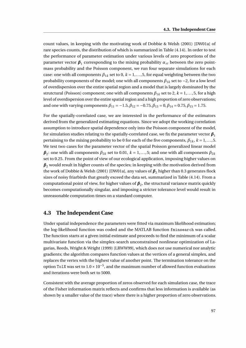
4.3. The Independent Case

count values, in keeping with the motivating work of Dobbie & Welsh (2001) [DW01a] of

rare species counts, the distribution of which is summarized in Table (4.14). In order to test

the performance of parameter estimation under various levels of zero proportions of the

parameter vector β1 corresponding to the mixing probability αst between the zero point-

mass probability and the Poisson component, we run four separate simulations for each

case: one with all components β1k set to 0, k = 1, . . . ,5, for equal weighting between the two

probability components of the model; one with all components β1k set to −2, for a low level

of overdispersion over the entire spatial region and a model that is largely dominated by the

strutctural (Poisson) component; one with all components β1k set to 2, k = 1, . . . ,5, for a high

level of overdispersion over the entire spatial region and a high proportion of zero observations;

and one with varying components β11 =−1.5,β12 =−0.75,β13 = 0,β14 = 0.75,β15 = 1.75.

For the spatially-correlated case, we are interested in the performance of the estimators

derived from the generalized estimating equations. Since we adopt the working correlation

assumption to introduce spatial dependence only into the Poisson component of the model,

for simulation studies relating to the spatially-correlated case, we fix the parameter vector β1

pertaining to the mixing probability to be 0 for each of the five components, β1k , k = 1, . . . ,5.

We test two cases for the parameter vector of the spatial Poisson generalized linear model

β2: one with all components β2k set to 0.01, k = 1, . . . ,5; and one with all components β2k

set to 0.25. From the point of view of our ecological application, imposing higher values on

β2 would result in higher counts of the species; in keeping with the motivation derived from

the work of Dobbie & Welsh (2001) [DW01a], any values of β2 higher than 0.3 generates flock

sizes of noisy friarbirds that greatly exceed the data set, summarized in Table (4.14). From a

computational point of view, for higher values of β2, the structural variance matrix quickly

becomes computationally singular, and imposing a stricter tolerance level would result in

unreasonable computation times on a standard computer.

4.3 The Independent Case

Under spatial independence the parameters were fitted via maximum likelihood estimation;

the log-likelihood function was coded and the MATLAB function fminsearch was called.

The function starts at a given initial estimate and proceeds to find the minimum of a scalar

multivariate function via the simplex-search unconstrained nonlinear optimization of La-

garias, Reeds, Wright & Wright (1999) [LRWW99], which does not use numerical nor analytic

gradients; the algorithm compares function values at the vertices of a general simplex, and

replaces the vertex with the highest value of another point. The termination tolerance on the

option TolX was set to 1.0×10−5, and the maximum number of allowed function evaluations

and iterations were both set to 5000.

Consistent with the average proportion of zeros observed for each simulation case, the trace

of the Fisher information matrix reflects and confirms that less information is available (as

shown by a smaller value of the trace) where there is a higher proportion of zero observations.

97


Table 4.1: Parameter and Data Generation Settings for Simulation Studies on the SpatialZero-Inflated Poisson Generalized Linear Model

Replications 500Number of Covariates q 5

Samples s 1000Starting Values β1 (0,0,0,0,0)

β2 (0,0,0,0,0)

Continuous Covariates X(s,q) ∼N (0,1) for all columns q = 1, . . . ,5Correlated Continuous Covariates X(s,q) ∼N (0,1) for columns q = 1,2,

X(s,3) = 0.9X(s,1)+0.8X(s,2)+ε, with ε∼N (0,1),X(s,q) ∼N (0,1) for columns q = 4,5

Independent Case: β1 (0,0,0,0,0)Mixing Probability Parameter (−2,−2,−2,−2,−2)

αst (2,2,2,2,2)(−1.5,−0.75,0,0.75,1.5)

Independent Case: β2 (0.3,0.3,0.3,0.3,0.3)Poisson Component Parameter

λst

Spatially-Correlated Case: β1 (0,0,0,0,0)Mixing Probability Parameter

αst

Spatially-Correlated Case: β2 (0.01,0.01,0.01,0.01,0.01)Poisson Component Parameter (0.25,0.25,0.25,0.25,0.25)

λst

Table 4.2: Results of Simulation 1.1.1: Independent Case with Continuous Covariates andβ10 = (0,0,0,0,0) Executed by Log-Likelihood Optimization.Average Proportion of Observed Zeros: 0.6876Average trace value of the Fisher information matrix: 3480.499

β10 β1 Mean Standard Error

0 β11 −0.0007 0.0990 β12 0.0056 0.1050 β13 −0.0048 0.1020 β14 −0.0050 0.1050 β15 −0.0033 0.106


0.3 β21 0.2999 0.0500.3 β22 0.2999 0.0510.3 β23 0.2976 0.0510.3 β24 0.2980 0.0490.3 β25 0.2982 0.051

For both continuous as well as correlated continuous covariates, we see that the zero-inflated

Poisson generalized linear model performs well in estimating each of the parameter vectorsβ1

and β2, with relatively low standard errors, which indeed cover the true value of the parameter.

98


Table 4.3: Results of Simulation 1.1.2: Independent Case with Continuous Covariates andβ10 = (−2,−2,−2,−2,−2) Executed by Log-Likelihood Optimization.Average Proportion of Observed Zeros: 0.6059.Average trace value of the Fisher information matrix: 5223.474.


−2 β11 −2.0723 0.341−2 β12 −2.0832 0.336−2 β13 −2.0845 0.342−2 β14 −2.0791 0.342−2 β15 −2.0932 0.334


0.3 β21 0.2986 0.0360.3 β22 0.2999 0.0330.3 β23 0.2962 0.0340.3 β24 0.3014 0.0360.3 β25 0.2988 0.035

Table 4.4: Results of Simulation 1.1.3: Independent Case with Continuous Covariates andβ10 = (2,2,2,2,2) Executed by Log-Likelihood Optimization.Average Proportion of Observed Zeros: 0.7661.Average trace value of the Fisher information matrix: 1524.525.


2 β11 2.0762 0.2882 β12 2.0670 0.2822 β13 2.0759 0.3032 β14 2.0571 0.3062 β15 2.0908 0.305


0.3 β21 0.3030 0.0690.3 β22 0.3056 0.0710.3 β23 0.3100 0.0660.3 β24 0.3084 0.0670.3 β25 0.3094 0.070

Table 4.5: Results of Simulation 1.1.4: Independent Case with Continuous Covariates andβ10 = (−1.5,−0.75,0,0.75,1.5) Executed by Log-Likelihood Optimization.Average Proportion of Observed Zeros: 0.6865.Average trace value of the Fisher information matrix: 3363.702.


−1.5 β11 −1.5392 0.191−0.75 β12 −0.7707 0.158

0 β13 0.0025 0.1450.75 β14 0.7608 0.161

1.5 β15 1.5251 0.189


0.3 β21 0.2958 0.0420.3 β22 0.2982 0.0440.3 β23 0.3004 0.0460.3 β24 0.3020 0.0460.3 β25 0.3013 0.047

We note in particular that the model performs well in estimating the parameter vector β1

that corresponds to the specification of the mixing probability αst , which thus provides a

satisfactory plausibility to fix the parameter vector β1 and test the performance of the model

comprising dependence for the spatially-correlated case in recovering values of the parameter

vector β2, corresponding to the Poisson parameter of the structural component of the model.

99


Table 4.6: Results of Simulation 1.2.1: Independent Case with Correlated Continuous Covari-ates and β10 = (0,0,0,0,0).Average Proportion of Observed Zeros: 0.6902.Average trace value of the Fisher information matrix: 7102.923.


0 β11 0.0128 0.1270 β12 0.0063 0.1230 β13 −0.0089 0.0920 β14 0.0023 0.1000 β15 0.0005 0.096


0.3 β21 0.3058 0.0580.3 β22 0.3027 0.0550.3 β23 0.2959 0.0420.3 β24 0.2992 0.0430.3 β25 0.2990 0.041

Table 4.7: Results of Simulation 1.2.2: Independent Case with Correlated Continuous Covari-ates and β10 = (−2,−2,−2,−2,−2).Average Proportion of Observed Zeros: 0.5851.Average trace value of the Fisher information matrix: 12282.843.


−2 β11 −1.9807 0.750−2 β12 −2.0167 0.748−2 β13 −2.0954 0.498−2 β14 −2.0512 0.592−2 β15 −2.0595 0.581


0.3 β21 0.3027 0.0550.3 β22 0.3008 0.0400.3 β23 0.2967 0.0310.3 β24 0.2999 0.0300.3 β25 0.3009 0.029

Table 4.8: Results of Simulation 1.2.3: Independent Case with Correlated Continuous Covari-ates and β10 = (2,2,2,2,2).Average Proportion of Observed Zeros: 0.7950.Average trace value of the Fisher information matrix: 1437.576.


2 β11 2.0957 0.4742 β12 2.0964 0.4642 β13 2.0992 0.3652 β14 2.0851 0.3802 β15 2.1074 0.383


0.3 β21 0.2944 0.1080.3 β22 0.3022 0.0960.3 β23 0.3079 0.0770.3 β24 0.2965 0.0730.3 β25 0.3056 0.074

4.3.1 Computing the Empirical Semivariogram

For the lattice case, we demonstrate how the Matheron method of moments estimator for

the semivariogram is computed. For 1000 observations, we assumed a 25×40 lattice and

partitioned the observation vector corresponding to simulated data for Simulation 1.1.1 across

the lattice to assign an observation to each point. The empirical semivariogram was then

100


Table 4.9: Results of Simulation 1.2.4: Independent Case with Correlated Continuous Covari-ates and β10 = (−1.5,−0.75,0,0.75,1.75).Average Proportion of Observed Zeros: 0.6688.Average trace value of the Fisher information matrix: 9054.700.


−1.5 β11 −1.4754 0.264−0.75 β12 −0.7233 0.215

0 β13 −0.0267 0.1660.75 β14 0.7673 0.167

1.5 β15 1.5211 0.202


0.3 β21 0.3025 0.0510.3 β22 0.3016 0.0480.3 β23 0.2966 0.0390.3 β24 0.3011 0.0370.3 β25 0.3047 0.041

computed according to Equation (1.3):

γ(‖h‖)= 1

2|s(‖h‖)|∑

(si ,s j )∈s(‖h‖)

(Z (si )−Z (s j )

)2

The Matheron method of moments empirical semivariogram is plotted against the distances

between points on the lattice in Figure 4.1. The flatness of the form is due to the indepen-

dence of the data, and reveals a variance of 1.5, which will be adopted for the value of the

overdispersion of the process in defining the spatial variance-covariance matrix to be inserted

in the quasi-score functions (to thus obtain the GEEs) associated with the parameter vector

β2, Equation (3.47).

Figure 4.1: Matheron method of moments empirical semivariogram for the independent case.

101


4.4 The Spatially-Correlated Case: The Matérn Correlogram

To incorporate spatial dependence into the model, as discussed in Section 3.5 of Chapter 3, we

augment the quasi-score functions associated with the parameter vectorβ, which corresponds

to the Poisson component of the model. This gives GEEs for the Poisson component of the

model which take the form of Equation (3.46),

SQuasiβ2

=∆sVar(ZStructural)−1(z−λ) = 0, (4.5)

where∆s = x>s Ds , the derivative component of the score functions corresponding to β2 with

xs = (xs1, · · · ,xsTs )> and Ds is given by Equation (3.30). The variance matrix of the structural

(Poisson) component is given by Equation (3.47),

Var(ZStructural) =Σ(ϕ,λ,ϑ,ν) =ϕV1/2µ R(ϑ,ν)V1/2

µ , (4.6)

where the entries of the diagonal matrix V1/2µ are given by the square root of the variance

functionp

v(·) for the Poisson component of the generalized linear model, for which we

assumed the canonical link, so√v(β2) =

√expx>stβ2. (4.7)

We implement a Matérn correlogram for the matrix R(ϑ,ν), given by a version of Definition

1.1.8 scaled by the variance of the process. It was remarked that when ν = 1.5, the Matérn

covariogram takes the convenient closed form of Equation (1.1); the correlogram for when

ν= 1.5 becomes

r (‖h‖) = (1+ϑ‖h‖)e−ϑ‖h‖ for ‖h‖ > 0. (4.8)

Taking advantage of the quasi-likelihood theory that needs only working assumptions (that

is, they need not be correct) of the covariance structure, for the simulation studies, we will

assume a value of ν= 1.5 and an arbitrarily-chosen value of ϑ= 0.25. Finally, as mentioned

previously in Section 4.3, the overdispersion parameter value will be set to ϕ= 1.5.

As for the score functions associated with the parameter vectorβ1, which pertain to the mixing

probability αst , we will take advantage of the lenience on the second-order structure property

of the quasi-likelihood theory and adopt the working assumption to leave them as is, of the

form of Equation (3.27). Moreover, as discussed in Section 3.5 of Chapter 3, this is a valid

working assumption, not just technically in terms of what quasi-likelihood theory allows,

but also motivated from an ecological application, or just from common sense: zero-valued

observations that arise from human or measurement error (sampling zeros), in principle, does

not affect zero-valued observations that arise from underlying characteristics of the stochastic

process explaining the nonzero observations (structural zeros).

102

4.4. The Spatially-Correlated Case: The Matérn Correlogram

The new score equations to be solved simultaneously allowing for spatial correlation, then, are

Sβ1=∑

s,tαst

((1−αst )

Prob(Zst = 0)(1−e−λst )1(zst = 0)−1(zst > 0)

)xst = 0, (4.9)

SQuasiβ2

=∆s(ϕV1/2

µ R(ϑ,ν)V1/2µ

)−1(z−λ) = 0. (4.10)

As discussed in Chapter 3, in order to use an optimization algorithm that comprises use of the

gradient, both score equations, Equations (4.9) and (4.10), need to be solved simultaneously

due to interdependence. Implementation in MATLAB requires the function fsolve which

searches for roots using a Newton method, while in R, the equivalent functions and packages

are nleqslv in the package nleqslv, multiroot in the package rootSolve, and sane in the

package BB solves large systems of nonlinear equations via nonmonotone Barzilai-Borwein

spectral methods. Optimization by searching for simultaneous solutions of the two score

equations is a significantly more difficult task that is vastly more computationally intensive

than by searching for the optimum of the log-likelihood function, which limits the application

of the model on standard computers. A technical direction for improvement would then be

to investigate more efficient methods of computation, and explore results of the domains of

numerical analysis and optimization towards the end of increased computational efficiency.

The results presented below are the estimates from one iteration of each covariate scenario and

parameter setting, numerous iterations would most certainly require access to a computing

cluster.

The component (block matrix) of the Fisher information matrix corresponding to the mixing

probability αst is given by Equation (3.38), while the variance of the corresponding to the

Poisson component of the model with the augmented score function is given by

Var(β2) =V −10 V1V −1

0 (4.11)

where V0 =∂µ>

s


−1s∂µs

∂β>2

(4.12)

V1 =∂µ>

s


−1s Var(Z)Var(ZStructural)

−1s∂µs

∂β>2

. (4.13)

The empirical variance-covariance of the outcome vector Var(Z) is given by (z−λ)(z−λ)>.

We see that despite the extended computation time and the intrinsic difficulty of the problem

of finding roots for a 10-variate function, the model was able to recover values for both

parameter vectors β1 and β2 quite well under both covariate scenarios. The recovery of

parameter values for the parameter vector β20 where all components were set to 0.01 was less

precise on different magnitudes, as the true parameter values are close to zero on an order of

two decimal places while the recovered estimates are close on an order of nine.

Upon closer investigation, we see that small values of β2 generate values of log(λst ) that are

also small, hence close to zero. This results in values of the parameter corresponding to the

103


Table 4.10: Results of Simulation 2.1.1: Spatially-Correlated Case with Continuous Covariatesand β20 = (0.01,0.01,0.01,0.01,0.01).

β10 β1 Estimate

0 β11 −1.60×10−09

0 β12 2.89×10−10

0 β13 1.56×10−09

0 β14 −2.61×10−11

0 β15 2.01×10−09

β20 β2 Estimate

0.01 β21 1.57×10−09

0.01 β22 1.22×10−09

0.01 β23 1.24×10−09

0.01 β24 3.07×10−09

0.01 β25 1.31×10−09

Table 4.11: Results of Simulation 2.1.2: Spatially-Correlated Case with Continuous Covariatesand β20 = (0.25,0.25,0.25,0.25,0.25).

β10 β1 Estimate

0 β11 4.58×10−06

0 β12 −2.12×10−06

0 β13 2.07×10−06

0 β14 1.47×10−06

0 β15 −2.74×10−06

β20 β2 Estimate

0.25 β21 2.478870×10−01

0.25 β22 2.489999×10−01

0.25 β23 2.478930×10−01

0.25 β24 2.500003×10−01

0.25 β25 2.500120×10−01

Table 4.12: Results of Simulation 2.2.1: Spatially-Correlated Case with Correlated ContinuousCovariates and β20 = (0.01,0.01,0.01,0.01,0.01).

β10 β1 Estimate

0 β11 3.08×10−10

0 β12 2.26×10−09

0 β13 3.80×10−09

0 β14 −6.13×10−10

0 β15 −5.57×10−09

β20 β2 Estimate

0.01 β21 3.86×10−09

0.01 β22 1.42×10−09

0.01 β23 7.07×10−09

0.01 β24 −6.92×10−09

0.01 β25 −2.76×10−09

Table 4.13: Results of Simulation 2.2.2: Spatially-Correlated Case with Correlated ContinuousCovariates and β20 = (0.25,0.25,0.25,0.25,0.25).

β10 β1 Estimate

0 β11 −1.40×10−10

0 β12 3.18×10−09

0 β13 −7.89×10−09

0 β14 −2.96×10−10

0 β15 3.18×10−09

β20 β2 Estimate

0.25 β21 2.500214×10−1

0.25 β22 2.499769×10−1

0.25 β23 2.500119×10−1

0.25 β24 2.499974×10−1

0.25 β25 2.500137×10−1

structural component of the model, the Poisson parameter, λst = expx>stβ2, which are close

to 1. Poisson random variables with a parameter value of 1 tend to be small, with a large

proportion of zeros, thereby increasing the overall proportion of zeros in the data, which,

104

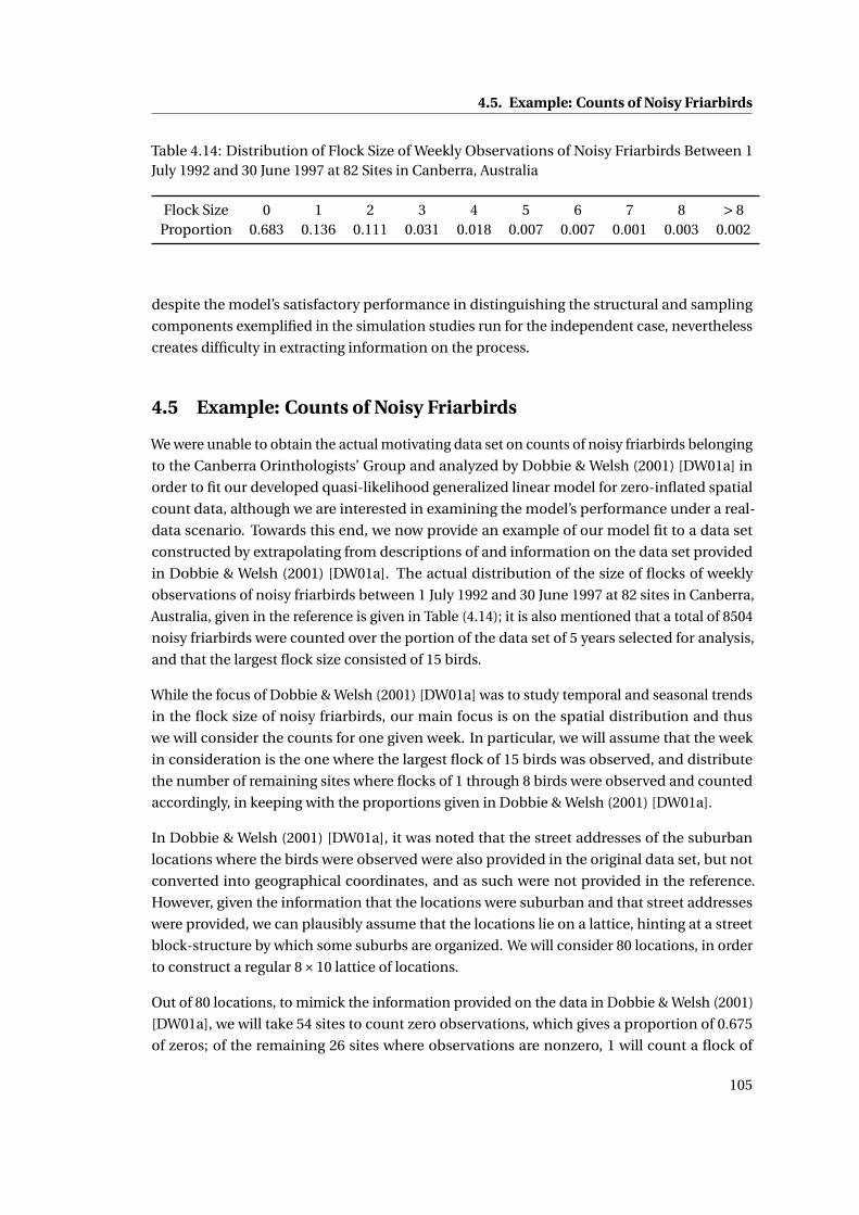
4.5. Example: Counts of Noisy Friarbirds

Table 4.14: Distribution of Flock Size of Weekly Observations of Noisy Friarbirds Between 1July 1992 and 30 June 1997 at 82 Sites in Canberra, Australia

Flock Size 0 1 2 3 4 5 6 7 8 > 8Proportion 0.683 0.136 0.111 0.031 0.018 0.007 0.007 0.001 0.003 0.002

despite the model’s satisfactory performance in distinguishing the structural and sampling

components exemplified in the simulation studies run for the independent case, nevertheless

creates difficulty in extracting information on the process.

4.5 Example: Counts of Noisy Friarbirds

We were unable to obtain the actual motivating data set on counts of noisy friarbirds belonging

to the Canberra Orinthologists’ Group and analyzed by Dobbie & Welsh (2001) [DW01a] in

order to fit our developed quasi-likelihood generalized linear model for zero-inflated spatial

count data, although we are interested in examining the model’s performance under a real-

data scenario. Towards this end, we now provide an example of our model fit to a data set

constructed by extrapolating from descriptions of and information on the data set provided

in Dobbie & Welsh (2001) [DW01a]. The actual distribution of the size of flocks of weekly

observations of noisy friarbirds between 1 July 1992 and 30 June 1997 at 82 sites in Canberra,

Australia, given in the reference is given in Table (4.14); it is also mentioned that a total of 8504

noisy friarbirds were counted over the portion of the data set of 5 years selected for analysis,

and that the largest flock size consisted of 15 birds.

While the focus of Dobbie & Welsh (2001) [DW01a] was to study temporal and seasonal trends

in the flock size of noisy friarbirds, our main focus is on the spatial distribution and thus

we will consider the counts for one given week. In particular, we will assume that the week

in consideration is the one where the largest flock of 15 birds was observed, and distribute

the number of remaining sites where flocks of 1 through 8 birds were observed and counted

accordingly, in keeping with the proportions given in Dobbie & Welsh (2001) [DW01a].

In Dobbie & Welsh (2001) [DW01a], it was noted that the street addresses of the suburban

locations where the birds were observed were also provided in the original data set, but not

converted into geographical coordinates, and as such were not provided in the reference.

However, given the information that the locations were suburban and that street addresses

were provided, we can plausibly assume that the locations lie on a lattice, hinting at a street

block-structure by which some suburbs are organized. We will consider 80 locations, in order

to construct a regular 8×10 lattice of locations.

Out of 80 locations, to mimick the information provided on the data in Dobbie & Welsh (2001)

[DW01a], we will take 54 sites to count zero observations, which gives a proportion of 0.675

of zeros; of the remaining 26 sites where observations are nonzero, 1 will count a flock of

105


Table 4.15: Constructed Distribution of Flock Size of Observations of Noisy Friarbirds for 1Week at 80 Sites

Flock Size 0 1 2 3 4 5 6 · · · 15

Number of Locations 54 10 8 3 2 1 1 0 1Proportion 0.675 0.125 0.1 0.0375 0.025 0.0125 0.0125 0 0.0125

15 noisy friarbirds, leaving 25 to associate flock sizes of 1 through 8 in accordance with the

true proportions given in Table (4.14), in Dobbie & Welsh (2001) [DW01a]. The distribution of

counts for our constructed data set is summarized in Table (4.15).

Since no information was provided in Dobbie & Welsh (2001) [DW01a] on the covariates other

than that a selection of what was provided in the original data set supplied by the Canberra

Orinthologists’ Group, we will generate them randomly according to the simulation studies

previously performed, and assume 5 continuous standard normal covariates provided at each

location, and thus parameter vectors β1 ∈ R5 and β2 ∈ R5 for the sampling and structural

components of the model, respectively.

Concerning the spatial covariance structure, no details were provided in Dobbie & Welsh

(2001) [DW01a] on the distribution of the counts over the spatial region, however, they adopt

the working assumption of an autoregressive correlation structure AR(1). For our constructed

data example, we will distribute the constructed counts presented in Table (4.15) over the

lattice and to increase the plausibility of the existence of a spatial dependence structure,

instead of randomly distributing the nonzero counts across the matrix, we will assume that

the locations where the counts are high lie in the upper left-hand corner of the lattice, and

arrange the counts to suggest positive spatial dependence. We segment the larger lattice into

a 2×2 block matrix, with dimensions of the (1,1) block are 5×6, those of the (1,2) block are

5×4, those of the (2,1) block are 3×6, and those of the (2,2) block are 3×4; each of the (1,2),

(2,1) and (2,2) matrices have all elements equal to zero, while the (1,1) block has the following

configuration: 4 6 3 2 1 1

5 15 3 2 1 0

4 3 2 2 1 0

2 2 2 2 1 0

1 1 1 1 1 0

Although this configuration does not suggest a weakly dependent nor isotropic correlation

structure, we will nevertheless take advantage of the lengience on the second-order structure

property of the quasi-likelihood and GEE theory to adopt the working assumption of a Matérn

correlation structure, as specified in Equation (4.8), with ϕ = 1.5, ν = 1.5 and ϑ = 0.25, in

keeping with the design of our simulation studies.

The results for the estimated parameter values recovered by the model are given in Table

106

4.5. Example: Counts of Noisy Friarbirds

(4.16). For the constructed data, the model estimates values of the components of β1 close to

zero, which corresponds to a value for the mixing probability αst of 0.5, suggesting that half

of the total probability model that generates the data is driven by the degenerate point-mass

distribution, while the other half is driven by a Poisson distribution with parameter given by

λst = expx>stβ2, where two of the components of the estimates are fairly low at two decimal

places away from zero, while the other three components are similar to the values that were

specified in the simulation design, which were chosen specifically to simulate data (counts or

flock sizes) that were similar to the data observed in Dobbie & Welsh (2001) [DW01a], as men-

tioned earlier. Moreover, we see from the results of Simulation 1.1.1 in Table (4.2), the scenario

that most closely resembles the parameter estimates recovered from the constructed noisy

friarbird data, that the average proportion of observed zeros is 0.6876, which is close to that

in the constructed data, 0,675. Since the parameter estimates recovered on the constructed

data set are similar to those used in the simulation studies, which indicated that the model

performs well, we conclude that the recovered parameter estimates on the constructed data

set in this example are satisfactory and likely to be close to the true parameters that generate

such observations for noisy friarbirds.

Table 4.16: Parameter Estimates for Constructed Noisy Friarbird Data.

β1 Estimate

β11 −0.005β12 −0.023β13 −0.074β14 −0.022β15 0.010

β2 Estimate

β21 0.12β22 0.06β23 0.32β24 0.31β25 0.04

107

5 Generating Point Processes for Zero-Inflated Spatial Data

In Section 1.3 of Chapter 1, the class of point pattern spatial data was introduced, where the

elements of a bounded region D , the locations si , i = 1,2, . . . ,n, occur randomly. As a data set,

these locations may feature patterns in their occurrence; the locations may exhibit complete

randomness, clustering, repulsion, or other regular pattern structures. A point process on Rd

is mathematically defined as a random variable N taking values in a measurable space (N,X ),

where N is the collection of all sequences si of points satisfying the local finiteness condition,

meaning that each bounded subset of Rd contains only finitely many points. The σ-algebra

X is defined as the smallest σ-algebra of subsets of N that defines the mappings ϕ 7→ϕ(x),

with x varying across the bounded Borel sets.

Augmenting this spatial location process to now allow covariate information to be associated

with each location, and observations to be measured at each location, generates marked point

processes. Marked point pattern analysis entails not only the study of collections of objects

randomly positioned in space, but also the marks associated with each object. These marks

provide additional information on each individual object (location) and may be quantitative

(continuous) or qualitative (discrete or categorical). The analysis and modeling of marked

point processes are often complex; one reason for this is that locations and marks are often

correlated. Examples of this behavior arise in many fields of science: in ecology, the number of

counts of a species occurring at a location may be affected by the availability and competition

for resources for survival at the location; in physics, the rotation velocity or strength of the

magnetic field of a supermassive black hole may depend on its location and the proximity of

other astrophysical objects in the sky. Another difficulty is the increased number of parameters

and moment structures since we are dealing with a combination of random processes and the

structures need to be defined for both components.

With the aim of constructing an algorithm for the simulation of zero-inflated Poisson processes

in space, in this chapter, we focus on the case of qualitative marked point processes. We outline

the foundations of and simulation algorithms for spatial point processes in the stationary

setting, and build on this compound structure and existing generation methods to motivate

a mixed, marked spatial point process to describe the behavior of spatially-varying species

109

Chapter 5. Generating Point Processes for Zero-Inflated Spatial Data

that are sited rarely in our ecological application. We propose stochastic zero-abundant mark

generation mechanisms for random locations, as well as for lattices.

5.1 Marked Point Processes

We will first outline in this section some basic theory on marked point processes to provide the

foundation for the models proposed in this chapter. What follows may be found in references

by Cox & Isham (1980) [CI80], Diggle (1983) [Dig83], Stoyan, Kendall & Mecke (1987) [SKM87],

Daley & Vere-Jones (2003) [DVJ88], Møller & Waagepetersen (2007) [MW07], Illian, Penttinen,

Stoyan & Stoyan (2008) [IPSS08] and Schneider & Weil (2008) [SW08], and in the book Case

Studies in Spatial Point Process Modeling (2006) [BGM+06], for example.

Definition 5.1.1. Let N be a point process on B ⊆D . A marked point process Z is a sequence

Z = (si ,m(si )

): si ∈ N

,

with points in B and mark space M , where m(si ) ∈M denotes the random mark attached to

the point (location) si ∈ B.

We consider M to be a finite set or subset of Rd , although more general cases exist and are

discussed by Stoyan & Stoyan (1994) [SS94] and Schlather (2001) [Sch01]. Multitype point pro-

cesses arise when M = 1,2, . . . ,k, i.e. when the marks correspond to k different categories of

points; more general point processes may be reduced to multitype point processes by binning

the mark space M accordingly. Multitype point processes are equivalent to multivariate point

processes when a k-tuple (Z1, Z2, . . . , Zk ) of point processes Z1, Z2, . . . , Zk corresponds to k

distinct types of points.

5.1.1 Marking Models

Marking models describe the behavior of the marks of a point pattern either a posteriori,

which explains how the marks in a pattern may have arisen given the marks, or a priori,

which explains how the marked points may have been generated. There has been much

development on marking models to describe a wide range of behavior relevant in various

applications, including ecology and forestry where interest lies in the evolution of plant

communities and tree populations depending on their growth in the presence of competition

for resources. Some propositions may be found in Pacala, Canham & Silander (1993) [PCS93],

Adler (1996) [Adl96], Berger & Hildenbrandt (2000) [BH00], Bugmann (2001) [Bug01], Dubé,

Fortin, Canham & Marceau (2001), Pretzsch (2002) [Pre05], Uriarte, Condit, Canham & Hubbell

(2004) [UCCH04], Särkkä & Renshaw (2006) [SR06], and Comas & Mateu (2007) [CM07].

Example 5.1.1. A simple way of generating stationary marked point processes is via the

independently marked or randomly labeled point process: the assumption underlying this

generation is that the locations are given a priori, while the marks are i.i.d. random variables

110

5.1. Marked Point Processes

according to some probability distribution. The construction of an independently marked

point process is defined by considering a stationary point process N = si together with a

sequence of i.i.d. random variables mi ; these two objects are combined arbitrarily to form

Z = (si ,m(si )

)where m(si ) = mi .

Independently marked point processes are often used for modeling in applications, such as

forestry and ecosystems. The Boolean model is a random set model which uses an independent

marking model; in a forestry application, the characteristics (marks) associated with remaining

trees in a managed forest exhibit random independent fluctuations, since those that exhibit

extreme characteristics (perhaps as a result of ecological competition for scarce resources) are

often removed. More details on the Boolean model can be found in Stoyan, Kendall & Mecke

(1987) [SKM87] and Molchanov (1997) [Mol95].

Example 5.1.2. The random superposition model is often used for point processes with quali-

tative marks, where the setting motivates the decomposition of the point process into subpro-

cesses generating nm ⊆ si , the collection of points with some fixed mark m. The subprocesses

are assumed independent and the entire marked point process is formed by their superposi-

tion, or their set-theoretic union. Such a construction indicates that the points in each of the

subprocesses nm are distributed according to some dependence behavior among points of

the same type, and are not affected by that among points of different types.

This behavior describes the two-component modeling assumptions of Dobbie & Welsh (2001)

[DW01a] where zeros and counts of noisy friarbirds are segregated, and could be used in

simulating conditional models for zero-inflated spatial point processes with counts. The

random superposition model generates population independence in the ecology literature,

such as by Goreaud & Pélissier (2003) [GP03] and Le Pichon, Gorges, Baudry, Goreaud & Boët

(2009) [LPGB+09].

Example 5.1.3. Correlated marks are generated by the random field model, proposed by Mase

(1996) [Mas96]. The marks associated with the points generated by a location process N = si

arise from an independent stationary random fieldY (s)

, where each mark m(si ) takes the

value m(si ) = Y (si ). The spatial dependence in the random field exhibits behavior in the

mark space M : if there is positive correlation inY (s)

then the points that are located within

proximity of one another tend to have similar marks.

Marking models may also be constructed by taking into account the geometry of the point

configuration in a certain neighborhood. One example is the nearest-neighbor distance dn(s),

the distance from the point s ∈ N to its nearest neighbor s1 ∈ N . Another example is the

number of other points within a distance a := ‖h‖ > 0 from s, na(s) = N (b(s, a))−1. Statistical

mark construction may also be implemented, where the marks take the form of a linear

function of the location plus some random fluctuation. One simple example of a statistically

constructed mark using the nearest-neighbor distance might be

m(s) = c0 + c1d(s)+ε(s),

111


where c0 and c1 are constants (parameters), and ε(·) is some random error. Such a construction

results in marked point processes with lower-valued marks in areas of high point density when

c1 > 0, and high-valued marks in areas of high point density when c1 < 0. More sophisticated

constructions also exist based on areas or volumes of Voronoi cells generated by a Dirichlet-

Voronoi tessellation of the point pattern, defined in Definition 1.3.7.

5.1.2 Motion Invariance

As with unmarked point processes (point pattern data) discussed in Section 1.3 of Chapter 1, a

definition of stationarity, analagous to Definition 1.3.3, also exists for marked point processes.

Also, as with each of the three types of spatial data discussed in Chapter 1, such an assumption

considerably simplifies the task of working with all the coordinates of the set D and may

be an unreasonable assumption to make, but a careful study of stationarity is an important

condition before approaching the more complicated case of nonstationarity.

Definition 5.1.2. A marked point process Z is stationary if and only if the process itself Z =(s1,m(s1)

),(s2,m(s2)

). . .

and the translated process Zs := (

s1+s,m(s1)),(s2+s,m(s2)

). . .

by

any vector s ∈ Rd are equal in distribution, i.e.

Zd= Zs for all s ∈ Rd .

Since a translated marked point process involves only translating the points (locations) si

while maintaining invariance of the marks m(si ), stationarity of a marked point process

Z = (si ,m(si )

): si ∈ N

implies stationarity of the unmarked point process N generating the

locations si . The definition of isotropy for marked point processes is analagous; see Definition

1.3.3. In general, for marked point processes, Euclidean motions of marked point processes

affect only the locations, but the marks remain unchanged.

The definition of stationarity provides insight as to what kind of marks may be suitable for

marked point pattern processes when we wish to make such an assumption on the process:

marks that are quantities relevant to the objects represented by the points (e.g. diameter,

height) or constructed marks (e.g. distance between the point and its nearest neighbor) pre-

serve stationarity of the process, while reference marks (e.g. distance between the point

and some point of reference or origin of the system of coordinates) will be perturbed under

translation.

Analagous to the intensity measure for unmarked point processes given in Equation (1.8), the

intensity measureΛ(·) of a marked point process Z is given by

Λ(B1 ×B2) = E[

Z (B1 ×B2)]

(5.1)

for two convex compact Borel sets B1,B2 ⊂ Rd . Under stationarity, for an unmarked point

process N , the intensity measureΛ(·) is a multiple of the Lebesgue measure µL(·) on Rd over

112


some convex compact Borel set B , Λ(B) = λµL(B) for the intensity λ of N , a nonnegative

constant, which has the interpretation as the mean number of points of N per unit volume as

defined in Equation (1.8). Analagously for stationary marked point processes, we have

Λ(B1 ×B2) =λµL(B1 ×B2) fM (m),

where fM (·) denotes the distribution of the marks.

5.1.3 First-Order Characteristics

For a marked point process under stationarity, the first-order characteristics concern both

the point process and the mark process. For the point process, the intensity λ introduced in

Definition 1.3.1 measures the mean number of points per unit area or volume. For the mark

process, if the marks are qualitative, then the mark probability pm is the probability that some

marked point has mark m.

Definition 5.1.3. Let M denote the random variable denoting the mark of a typical point, then

the mark probability is determined by the relative intensity

pm = Prob(M = m) = λm

λfor m = 1,2, . . . ,

where λm is the intensity of the subprocess Nm of N , which generates the points nm with mark

m.

The mean number of points of the marked point process Z (·) in the set B with the mark m is

E[

Z(B × m

)]=λpm |B |. (5.2)

The case of quantitative marks entails the construction of the mark distribution function fM (·)to determine the distribution of the marks independently of the positions of the points, whilst

maintaining probabilistic properties in order to assure well-posedness and correct definition.

Since our setting concerns only qualitative marks, we refer the interested reader to Illian,

Penttinen, Stoyan & Stoyan (2008) [IPSS08], for example, for a mathematical derivation.

Under stationarity, the following theorem due to Campbell (1909) [Cam09] provides a concise

expression for the computation of the mean of a marked point process. More generally,

Campbell’s theorem provides the moment generating function for a shot noise process, from

which the mean and variance may be computed in a straightforward manner by solving a

volume integral.

Theorem 5.1.4 (Campbell, 1909 [Cam09]). For a marked point process, the mean expression

113


can be computed by

E

[ ∑(s,m(s))∈Z

fZ(s,m(s)

)]=λ∫

Rd

∑m

pm fZ (s,m)ds =λ∑m

pm

∫Rd

fZ (s,m)ds.

5.1.4 The Palm Distribution Revisited

From the definition of the Palm distribution given in Chapter 1, Definition 1.3.4, together with

a version of Campbell’s theorem given in Theorem 5.1.4 for unmarked point processes, the

Palm mean Eo[·], important in the subsequent definitions of second-order characteristics, may

be defined. The resulting formulation which gives this mean is known as the Campbell-Mecke

formula:

E

[ ∑s∈N

fN (s, N )

]=λ

∫Rd

Eo[

fN(s, (N −s)

)]ds =λEo

[∫Rd

fN(s, (N −s)

)ds

], (5.3)

where (N −s) denotes the point process translated by s, as in Definition 1.3.4. Note here that

the distribution of the points fN (·, ·) depends not only on s but also the other points of the

process N .

Palm distributions ProbM (·) may also be defined for mark spaces M ⊆ R, which give the

conditional distribution and expectation of Z , given that there is a point of Z with mark

m ∈ M at the origin o. Analagously to Definition 1.3.4, the Palm distribution for a marked

point process Z with marks m taking values in the mark space M and some marked point

occurring at the origin o may be defined by

λVol(W )ProbM (Z ∈A ) = E

[ ∑(s,m(s))∈Z

1(s ∈W )1(m(s) ∈M )1((Z −s) ∈A

)], (5.4)

where as before in Definition 1.3.4, W is some test set, and Z ∈A indicates that the marked

point process Z has some well-defined property A . The general definition given by the above

of the Palm distribution may be refined so that the marked point occurring at the origin o is of

the particular type m, which allows Equation (5.4) to be written as

ProbM (Z ∈A ) =∫B

Prob(o,m)(Z ∈A ) fM (m)dm. (5.5)

The Palm mean E(o,m)[·] for marked point processes is given by an appropriate adaptation of

the Campbell-Mecke formula in Equation (5.3). For some function f (·, ·, ·) that depends on a

point s ∈ Rd , a mark m ∈ R, and a stationary marked point process Z ,

E

[ ∑(s,m(s))∈Z

f(s,m(s), Z

)]=λ∫

Rd

∫ +∞

−∞E(o,m)

[f(s,m, (Z −s)

)]fM (m)dmds, (5.6)

where E(o,m)[·] denotes the expectation with respect to the Palm distribution where the marked

114


point occuring at the origin o has mark of particular type m, Prob(o,m)(·).

5.1.5 Second-Order Characteristics

Second-order characteristics are useful statistics for describing the variability of data; in the

context of marked point processes, these entail describing not only the variability of the point

process driving the random locations and that of the marks associated with each location,

but also the correlations between marks and points. A selection of second-order variability

measures for point processes with qualitative marks are given here; measures for quantitative

marks may be found in the aforementioned references.

Multivariate K Functions

Ripley’s K function defined in Equation (1.13) as a measure of complete spatial randomness

may be extended to the multivariate setting. The multivariate K function, Kml (·), is defined by

λl Kml (a) = Eom[Nl

(b(o, a)

)]for a ≥ 0,

where Eom[·] denotes the expectation under the Palm distribution for marks of type m, or the

conditional expectation that the point located at o is of type m. λl Kml (a), then, is the mean

number of points of mark type l in a ball of radius a centered at some point of mark type m.

When m 6= l , the point at o is excluded; when m = l , Kml (a) is reduced to Km(a), the univariate

K function for the subprocess Nm . By definition of Kml (·), we have Kml (a) = Klm(a) for r ≥ 0.

In considering disassociations between points and marks, condensed Kml (·) functions Km·(a)

and K·l (a) may be considered, respectively. Formally, for a ≥ 0, they are given by

λKm·(a) = Eom[N

(b(o, a)\o

)]⇐⇒ Km·(a) =∑l

pl Kml (a), (5.7)

λl K·l (a) = Eom[Nl

(b(o, a)\o

)]⇐⇒ K·l (a) =∑m

pmKml (a), (5.8)

where recall that pl = λl /λ. The left-hand side of the equivalence of Equation (5.7) counts

the mean number of points independent of their marks in a ball of radius a centered at some

point of mark type m, excluding this point of reference. In the same manner, the left-hand

side of the equivalence of Equation (5.8) counts the mean number of points of type l in a ball

of radius a centered at some point, independent of its mark.

As with motion invariance, the underlying motivation defining K functions and their multi-

variate counterparts may provide insight on the use of marking model. Under independent

marking, then all the condensed K functions coincide, i.e. Kml (a) = K (a) for all m and l , where

K (·) denotes the K function for the point process N , independent of the marks. Under random

superpositioning, Kmm(a) = Km(a) where Km(·) is the K function for the subprocess Nm , and

Kml (a) = Vol(b1)d ad for m 6= l . Values for the functions Kml (·) that do not coincide when the

115


indices do not coincide signifies correlation between marks.

Cross-Pair Correlation Functions

The pair correlation function rpair(·) defined in Equation (1.14) may be extended to Rd as

follows:

r pair(a) = 1

Vol(b1)d ad−1

dK (a)

d a. (5.9)

For multivariate point processes, this correlation function is extended by defining the prod-

uct densities ρml (·); in keeping with the construction discussed in Example 1.3.1, the term

ρml (a)dxdy gives the probability that a point of type m occurs in an infinitesimally small ball

b(x) with volume dx, and that a point of type l occurs in an infinitesimally small ball b(y) with

volume dy, where the distance between the centers of the two balls is a. As for the multivariate

K functions, whenever m = l , the second-order product density ρ2(·) for the subprocess Nm

is obtained, and ρml (a) = ρlm(a) for all m, l , and a ≥ 0. Analagous to the construction given

in Example 1.3.1, the cross-pair correlation functions may be defined in terms of ρml (·) by

normalizing to obtain

r pairml (a) = ρml (a)

λmλlfor a ≥ 0. (5.10)

The symmetry of the product densities ρml (·) = ρ(·) implies the symmetry of the cross-pair

correlation functions r pairml (a) = r pair

l m (a) for all m, l , and a ≥ 0. Similar to the definition of the

pair correlation function given in Equation (1.14), the cross-pair correlation function also has

a representation in terms of the derivative of the multivariate K function,

r pairml (a) = 1

Vol(b1)d ad−1

dKml (a)

d afor a ≥ 0. (5.11)

As with the pair correlation function defined in Equation (1.14), we have have r pairml (a) ≥ 0 for

all a ≥ 0, and lima→∞ r pairml (a) = 1 for all m and l .

Along with motion invariance and the definition of the multivariate K functions, the cross-

pair correlation functions are helpful in determining which marking model to use. Under

independent marking, the product densities ρml (·) are defined by ρml (a) = pm plρ(a) and the

cross-pair correlation functions r pairml (·) are given by r pair

ml (a) = r pair(a) for a ≥ 0, where r pair(·)is the pair correlation function of the point process N , defined as in Equation (1.14). Under

random superpositioning, we have r pairmm(a) = r pair

m (a) and r pairml (a) = 1 whenever m 6= l , where

r pair(a) is the pair correlation function for the subprocess of points Nm .

116


Mark Connection Functions

A conditional approach to analyzing the correlation between two points is given by mark

connection functions pml (a), which dictates the conditional probability for two given points

in the point process N , that two points at a distance a ≥ 0 from one another have marks m

and l . Under motion invariance, we can pick the two points to be o and a, where a is any point

at a distance a ≥ 0 from o. The mark connection function is then defined by

pml (a) = Proboa(m(o) = m,m(a) = l

),

where Proboa(·) denotes probability under the Palm distribution. Empirically, mark connec-

tion functions are computed in terms of the partial correlation functions ρml (·); we have

pml (a) = ρml (a)

ρ(a)= pm pl

r pairml (a)

r pair(a)for a > 0,

for well-posedness. When a = 0, we set pmm(0) = 1 and pml (0) = 0 whenever m 6= l by means

of the cross-pair product density, ρml (·). Studying the asymptotic behavior of the mark

connection function gives the range of the mark correlation, lima→∞ pmm(a) = p2m and we

have lima→∞ pml (a) = 2pm pl when m 6= l .

Under independent marking, the asymptotics of the mark connection function define the

conditional probabilities, and we have pmm(a) = p2m and pml (a) = 2pm pl when m 6= l . Under

random superpositioning, we have

pmm(a) = λ2mr pair

m (a)

λ2mr pair

m (a)+λ2l r pair

l (a)+2λmλl

and pml (a) = 2pm pl for m 6= l , where r pairm (·) is the pair correlation function for the subprocess

Nm .

Another conditional approach was proposed by Shimatani (2001) [Shi01], which considers the

probability that two points at a given distance a > 0 from one another have marks different

from m by

pm(a) = 1−pmm(a).

5.1.6 Other Complexities of Spatial Point Processes: Interaction Models

More complicated models exist for both unmarked and marked spatial point pattern processes,

involving interaction among the points; one important class is that of Markov point processes,

which are also known as Gibbs point processes in the statistical physics literature, such as in

Ruelle (1969) [Rue69], where the concept was first derived. Such processes are constructed

by constructing a density on a point process with respect to a Poisson process in such a way

that a Markov property holds, thus enabling attraction or repulsion behavior to be modeled

117


within a spatial point process. The foundations, theory, construction and illustrations by

applications of Markov point processes has been comprehensively and concisely documented

by Van Lieshout (2000) [vL00].

A particular case of Markov point processes is that of the pairwise interaction process, where

the correlation among the points are modeled additively by considering pairwise interactions,

which will be revisited further on in this chapter in the construction of a zero-inflated marked

Poisson process. Behavior that is more general than pairwise interaction is captured by area-

interaction point processes, constructed by Baddeley & Van Lieshout (1995) [BvL95]. Marks,

local scaling, clusters, inhomogeneity and extensions to Rd further build upon the complexity

of these types of processes, which have been discussed by Stoyan, Kendall & Mecke (1987)

[SKM87], Møller & Waagepetersen (2007) [MW07], Schneider & Weil (2008) [SW08], and in the

book Case Studies in Spatial Point Process Modeling (2006) [BGM+06].

5.2 Simulating Spatial Point Processes

Historically speaking, simulation of spatial point processes were first established in the field

of statistical mechanics via Metropolis-Hastings algorithms, for example by Metropolis, Rosen-

bluth, Rosenbluth, Teller & Teller (1953) [MRR+53], Norman & Filinov (1969) [NF69] and

Zamalin, Filinov & Norma (1977) [ZNF77], although the more recent work of Ripley (1976)

[Rip76], Ripley & Kelly (1977) [RK77] and Baddeley & Møller (1989) [BM89] on simulation

by spatial birth and death processes have been long considered as the classical simulation

methods. The most recent breakthrough resulted in perfect or exact simulation, pioneered by

Propp & Wilson (1996) [PW96], which then gave rise to a multitude of perfect samplers based

on spatial birth and death models for the simulation of spatial point processes.

In this section, we outline the three simulation methods and propose the inclusion of zero-

inflation methods to generate zero-inflated spatial point processes.

5.2.1 Metropolis-Hastings Algorithms

Metropolis-Hastings algorithms form a class of MCMC method to obtain random samples for

probability distributions from which direct sampling is difficult. In the case of spatial point

processes, often densities are nonnormalized, i.e. global, joint densities are expressed up to

a constant of proportionality, which are often unknown or difficult to compute such as in

Theorem 1.2.3. An example to illustrate this difficulty involves considering a spatial Poisson

process Y ∼P (λ) over D , with mean surface µ(D) =∫Dλ(s)ds <+∞; the density (probability

mass function) of the Poisson process is then

fY (y) = exp|D |−µ(D)

∏s∈y

λ(s). (5.12)

118

5.2. Simulating Spatial Point Processes

As is the case in Theorem 1.2.3, often the densities are only specified up to a constant of

proportionality, so fY (·) ∝ gY (·) where gY : ΩD → R+ is a known function that maps from

the set of finite point configurations ΩD = y ⊂ D : |y| < +∞ (cf. Definition 1.2.2) to the

nonnegative real numbers R+. The normalizing constant or partition function (the latter

expression belongs to the terminology of statistical mechanics) c is then

c =∞∑

j=0

exp−|D |

j !

∫Dd

gY(y1,y2, . . . ,yn

)dy1 · · ·dyn . (5.13)

The specification of nonnormalized distributions as target distributions thus often calls for the

implementation of such an MCMC algorithm. MCMC algorithms such as Metropolis-Hastings

generate Markov chains, previously discussed in Section 1.2.2 of Chapter 1, and defined in

Equation (1.2.2), which form a sample of “approximate simulations” of some specified target

distribution, which tends towards the target distribution itself as the number of samples

tends towards infinity. Common Metropolis-Hastings algorithms for the simulation of spatial

point processes are reversible in reference to the target distribution, meaning that if some

random variable X is distributed according to the target distribution, then the pairs (Xn , Xn+1)

and (Xn+1, Xn) are identically distributed, and irreducible, meaning that the Markov chain

generated can attain any state irrespective of the starting point. Reversibility in reference to

the target distribution and irreducibility together imply that the limiting distribution of the

Markov chain, if it exists, is necessarily the target distribution; irreducibility, in particular,

establishes convergence of the Markov chain, and implies consistency of the Monte Carlo

estimates.

Geyer & Møller (1994) [GM94] provide alternative simulation procedures for marked point

processes on a general state space using a Metropolis-Hastings algorithm. For a marked

Poisson process with nonnormalized density gX (·) on D ×M where D ⊆ Rd with |D | < +∞and M ⊆ Rd , and intensity λ(·, ·) given by some density on M , λ

(s,m(s)

) = fM (m), a Gibbs

sampling scheme applied to a continuum Ising model generates a marked point process.

The Ising model was originally introduced in the field of statistical mechanics by Ising (1925)

[Isi25] as a mathematical model for ferromagnetism. With the goal of finding phase transitions,

the model consists of a set of binary variables representing the spin states of an electron,

−1,+1 (up or down) arranged on a graph, usually a lattice, where each spin interacts with its

nearest neighbors on the lattice vertices. Numerical simulations to generate configurations of

spins are carried out using a Metropolis-Hastings algorithm with respect to a Gibbs distribution

with inverse temperature η= 1/T and computing the energy contribution ∆E according to the

energy function E (·); see Definition 1.2.5. The algorithm proceeds as follows:

Algorithm 5.2.1 (Metropolis algorithm for numerical simulations of the Ising model.).

1. Pick a spin at random and compute the contribution to the energy involving this spin

119


and its nearest neighbors only;

2. Flip the value of the spin and compute the new contribution ∆E ;

3. If the new energy is less, keep the new spin;

4. If the new energy is more, retain the new spin only with probability exp−η∆E ;

5. Repeat.

Georgii & Häggström (1996) [GH96] propose an analagous continuum Ising model by consid-

ering a class of bivariate point processes with densities of the form

fZ (z1,z2) ∝βN (z1)1 β

N (z2)2

∏z∈z1

∏ζ∈z2

ι(z,ζ) (5.14)

for parameters β1 > 0, β2 > 0 and where 0 ≤ ι(·) ≤ 1 is an interaction function for some pairwise

interaction process X with density

fX (x) ∝ ∏ξ∈x

ι(ξ)∏

ξ,χ⊆xι(ξ,χ

),

for ξ,χ ∈ x ⊆D , i.e. ι(·) is a nonnegative function which renders the right-hand side integrable

in the context of a Poisson process. The interaction function may also be defined in terms

of cliques, by Definition 1.2.5: An interaction function ι :ΩD → R+ is one such that if ι(x) 6= 1

implies that x is a clique.

Example 5.2.1. An example of a simple yet nontrivial pairwise interaction process is the

Strauss process due to Strauss (1975) [Str75], with interaction function given by

ι(a) = γ1(a≤R), (5.15)

setting 00 = 1 by default. Here, γ ∈ [0,1] is an interaction parameter, and R > 0 is the range of

interaction. The density takes the form

fX (x) ∝βN (x)γsR (x)

where β > 0 is a parameter and sR (x) = ∑ξ,χ⊆x 1

(‖ξ−χ‖ ≤ R)

is the number of pairs at a

distance R apart in x.

If γ= 1, we obtain a Poisson process, while for γ< 1, there is repulsion between the pairs of

points at a distance R apart in X . The special caise where γ= 0 is known as a hard core process

with hard core R, since the points cannot be closer than R apart; realizations of a Strauss

process appear more and more regular as γ decreases.

Example 5.2.2. The Strauss process has been extended to a multiscale process by Penttinen

(1984) [Pen84] where the interaction function takes the form

ι(a) = γi if Ri−1 ≤ a ≤ Ri , (5.16)

120


with segmenation 0 = R0 < R1 < ·· · < Rk < Rk+1 = +∞ for k ∈ N, γi > 0, i = 1,2, . . . ,k and

γk+1 = 1, so that the process has range of interaction R = Rk . THe density takes the form

fX (x) ∝βN (x)k∏

i=1γ

si (x)i ,

with si (x) = ∑ξ,χ⊆x 1

(Ri−1 ≤ ‖ξ−χ‖ ≤ Ri

). For k = 1, the multiscale process reduces to a

Strauss process.

The reference of Georgii & Häggström (1996) [GH96] also mentions further extensions of

interactions for pairs of points of the same type and issues of uniqueness and phase transition

for infinite extensions. Extending Equation (5.14) to k-variate point processes, the density

then becomes

fZ (z1,z2, . . . ,zk ) ∝k∏

i=1β

N (zi )i

∏ζ1∈z1

· · · ∏ζk∈zk

ι(ζ1,ζ2, . . . ,ζk ) (5.17)

where 0 ≤ ι(ζ1,ζ2, . . . ,ζk ) ≤ 1.

The technique of Gibbs sampling was previously discussed in detail in Section 1.2.2 of Chapter

1, specifically on page 37. This algorithm may be extended to a k-component Gibbs sampler by

means of the conditional distributions on a set A ⊆D

Z1|(Z2, . . . , Zk ) ∼P (λ1,Z2,...,Zk ), · · ·Zk |(Z1, . . . , Zk−1) ∼P (λk,Z1,...,Zk−1 ), (5.18)

where

λ1,Z2,...,Zk (z) =β1∏ζ2∈Z2

· · · ∏ζk∈Zk

ι(z,ζ2, . . . ,ζk )

...

λk,Z1,...,Zk−1 (z) =βk

∏ζ1∈Z1

· · · ∏ζk−1∈Zk−1

ι(ζ1, . . . ,ζk−1,z).

Algorithm 5.2.2 (Gibbs sampler for a continuum Ising model, Geyer & Møller (1994) [GM94]).

Using a cyclic updating scheme, we generate a Markov chain Zm = (Zm,1, Zm,2, · · · , Zm,k ) where

m ∈ Z+ such that over a set A,

1. Zm+1,1|(Zm,2, . . . , Zm,k ) ∼P (λ1,Zm,2,...,Zm,k )

2. Zm+1,2|(Zm+1,1, Zm,3, . . . , Zm,k ) ∼P (λ2,Zm+1,1,Zm,3,...,Zm,k )...

k. Zm+1,k |(Zm+1,1, . . . , Zm+1,k−1) ∼P (λk,Zm+1,1,...,Zm+1,k−1 ).

121


5.2.2 Simulation Based on Spatial Birth and Death Processes

The fact that under suitable conditions, spatial birth and death processes, if run for sufficiently

long, generate realizations of a finite point process was first noticed by Ripley (1976) [Rip76],

Ripley & Kelly (1977) and Preston (1977) [Pre74], and discussed later on in detail by Baddeley &

Møller (1989) [BM89], which then came to be considered as the standard simulation method

in the field of point processes. Birth and death processes present a special case of a continuous

time Markov process, where the size of the current population represent the states of the

process, and the transition mechanisms from state to state are limited to births and deaths;

when a birth occurs, the process transitions from state n to state n +1, while when a death

occurs, the process transitions from state n to state n −1.

Definition 5.2.1. The distribution of a spatial birth and death process X t ∈ F with t ∈ R+may be defined by a governing birth rate b(·, ·) and death rate d(·, ·), which are nonnegative

functions onΩD ×D . For x ∈ΩD , define

β(x) =∫D

b(x,ξ)dξ,

δ(x) = 0 if x =∅∑

ξ∈xd(x\ξ,ξ) if x 6=∅

α(x) =β(x)+δ(x). (5.19)

We assume that β(x) <∞ for all x ∈ΩD .

• For β(x) > 0, define a probability density function bX (x, ·) on D by bX (x,ξ) = b(x,ξ)

β(x).

• For δ(x) > 0, define a probability mass function dX (x, ·) on D by dX (x,χ) = d(x\χ,χ)

δ(x).

The spatial birth and death process X t , t ≥ 0, is a right-continuous and piecewise constant

except at specific jump times T1 < T2 < ·· · and jumps defined in the following manner: For the

initial state x0 ∈F , set

T0 = 0,

X0 = x0,

Jn = XTn ,

for states n = 0,1,2, . . .. Conditioning on J0,T0, J1,T1, . . . , Jn ,Tn , where Jn = x, and with α(x) > 0

gives

Tn+1 −Tn ∼ Exp(α(x)

),

where Exp(ε) denotes the exponential distribution with parameter ε > 0 with probability

density function fY (y ;ε) = εe−εy 1(y ∈ R+).

122


Conditioning further on Tn+1 means that either a birth or a death occurs at time Tn+1, where

• a birth occurs with probabilityβ(x)

α(x), the jump Jn+1 is defined by Jn+1 = x∪ξn , where the

new birth point ξn is generated by the density bX (x, ·); and

• a death occurs with probabilityδ(x)

α(x), the jump Jn+1 is defined by Jn+1 = x\χn , where the

point to be deleted χn from x is chosen by the density dX (x, ·).

By this construction, the jump chain J0, J1, J2, . . . is a Markov chain. Moreover, the Markov

property of “memorylessness” of the exponential distribution due to the implication that

T − t |T > t ∼ Exp(ε) if T ∼ Exp(ε) for ε> 0 and t > 0 renders the spatial birth and death process

X t a continuous time Markov process, meaning that for any time t ≥ 0, given X t = z and the

past history Xs for s < t , the waiting time to the first jump in Xu for u > t is exponentially-

distributed with parameter α(x) and the distribution of the jump is still given by either a birth

or a death as defined in the above Definition 5.2.1.

For the well-posedness of the spatial birth and death process in Definition 5.2.1, the cases

of absorption and explosion need to be addressed. When α(x) = 0, the birth and death rates

are offset exactly and absorption occurs, and we declare Xu = x for u ≥ Tn and Tk =∞ for

k > n; absorption will be disregarded since it is not relevant for the simulation of spatial point

processes. When an infinite number of jumps may occur with positive probability in a finite

time interval, the process is said to explode; we will similarly disregard the case of explosion

of spatial birth and death processes, which is feasible via technical sufficient conditions (see

Møller & Waagepetersen (2007) [MW07]).

Algorithm 5.2.3 (Algorithm for the simulation of a spatial birth and death process, Møller

& Waagepetersen (2007) [MW07]). For n = 0,1,2, . . ., initialize (Tn , Jn) = (t ,x) and α(x) > 0.

Where Unif([0,1]

)denotes the uniform distribution on the interval [0,1], generate (Tn+1, Jn+1)

by

1. Sample R ′n ∼ Unif

([0,1]

)and R ′′

n ∼ Unif([0,1]

);

2. Compute Tn+1 = t + log(−R ′n)

α(x);

3. If R ′′n ≤ β(x)

α(x), sample ξn ∼ bX (x, ·) and put Jn+1 = x∪ξn ;

4. Otherwise, choose χn to delete by sampling χn ∼ dX (x, ·) and put Jn+1 = x\χn .

R ′n , R ′′

n , and ξn or χn are mutually independent, given the random variables used to generate

(T0, J0, . . . ,Tn , Jn).

The above algorithm described in Example 5.2.3 can be slow, since β(x) needs to be computed

and new birth points ξn need to be sampled from bX (x, ·). The speed of the algorithm may

123


be improved by “embedding” the birth probability density function in a larger class, which

is easier to compute; i.e. we suppose that some b(x, ·) exists such that b(x,ξ) ≤ b(x,ξ) for all

ξ ∈F , and such that β(x) =∫D

b(x,ξ)dξ<∞ is easy to compute, and such that it is easy to

sample from b(x, ·) = b(x, ·)/β(x). An alternate algorithm can then be constructed to generate

a spatial birth and death process; see Møller & Waagepetersen (2007) [MW07] for details.

Simulation of a Spatial Point Process from a Spatial Birth and Death Process

The algorithm presented in Example 5.2.3, as well as its faster equivalent referenced in Møller

& Waagepetersen (2007) [MW07] can be used for the simulation of spatial point processes N

with nonnormalized density with respect to a Poisson process over the set A ⊆D . We assume

that for all x ∈ΩD and ξ ∈A \z,

gN (x)bN (x,ξ) = gN (x∪ξ)dN (x,ξ). (5.20)

This is a detailed balance condition that provides reversibility with respect to gN (·) with the

additional assumption that E[β(X )

]<∞, by the following proposition.

Proposition 5.2.2. Under the detailed balance condition of Equation (5.20) and a finite ex-

pectation E[β(X )

]<∞ where X ∼ gX (·), then X t with t ≥ 0 is reversible with respect to gX (·),

i.e. if X0 ∼ gX (·) for any t > 0, the processes Xs with 0 ≤ s ≤ t and X t−s ≤ s ≤ t are identically

distributed.

The proof is provided by Møller & Waagepetersen (2007) [MW07].

From the detailed balance condition of Equation (5.20), we also obtain the fact that if X0 ∈S := x ∈ΩD : gX (x) > 0, the natural state space of the chain, then X t ∈S for all t ≥ 0. Under

the additional assumption that if

x∪ξ ∈S implies that the death rate dN (x,ξ) > 0, (5.21)

then gX (·) is hereditary according to Definition 1.3.6, by construction. In addition, by the

detailed balance condition, α(∅) = 0 if S =∅, since

α(∅) =∫

AbN (∅,ξ)dξ= 1

gX (∅)

∫A

gX (ξ)dN (∅,ξ)dξ

and α(x) > 0 for all x ∈ S if S 6=∅. Irreducibility is also provided by the detailed balance

condition of Equation (5.20) and Condition (5.21), since the process can transition from any

state in S to ∅, and vice versa, from ∅ to any state in S . Given reversibility, heredity, and

irreducibility, under further weak assumptions the process X t converges to N , as with the case

of associated Markov chains generated by Metropolis-Hastings algorithms discussed above.

124


5.2.3 Perfect Simulation

In terms of algorithms for Markov chains, exactness is said to be attained if the algorithm

returns exact draws from a given target distribution at its completion; the running time of the

algorithm may be random, but is nevertheless usually finite. In practice, however, exact algo-

rithms will often exhibit limitations due to random number generators, and while the running

time is finite, it may not return an answer within reasonable time frames. Because of these

limitations, the term perfect simulation was adopted by Kendall (1998) [Ken98] and Kendall

& Møller (2000) [KM00] to signify exact simulation in practice, although both terms exist in

the literature. Perfect simulation is a particularly advantageous simulation method since it

overcomes the issue of initialization to obtain an appropriate burn-in, i.e. the initialization

of the algorithm followed by sufficiently many iterations until the initial state is “forgotten”.

Additionally, perfect simulation provides i.i.d. samples, so asymptotic Monte Carlo estimates

can easily be computed. The comparison of a perfect simulation algorithm with its nonperfect

counterpart also allows the approximation error to be determined.

Propp & Wilson (1996) [PW96] propose a coupling from the past (CFTP) technique that gen-

erates a class of algorithms that provide perfect simulation. Its application to spatial point

process setting, however, is difficult, due to technical limitations, though the contribution

nevertheless has innovatively inspired the development of numerous perfect samplers for

spatial point processes based on the spatial birth and death process approach discussed earlier.

For completeness, we provide a general overview of CFTP algorithms and the special-case

Propp-Wilson algorithm, and mention its limitations in modeling spatial point processes; we

also provide a list of references of perfect samplers for spatial point processes.

Coupling From the Past (CFTP) Algorithms and the Propp-Wilson Algorithm

The construction of a discrete time Markov chainYn

∞n=0 with invariant distributionΠ on a

state spaceΩ=⋃∞i=0

x ∈D : N (x) = i

can be obtained by a stochastic recursive sequence (SRS)

Yn+1 = Yn)ג ,Rn) for n ∈ Z+, (5.22)

where Rn , n ∈ Z+, are i.i.d. random variables and (·)ג is a deterministic updating function.

Technical specifications and conditions on the SRS and updating function are given in Foss &

Tweedie (1998) [FT98], though in practice, the updating function (·)ג is provided numerically

and Rn are generated via pseudorandom numbers. Negative times are allowed, and for x ∈S

and n ≤ q , the state of a chain that starts at x at time n is denoted at time t by

Y tn (x) =

x if n = t ,

ג(· · Rn+1,(x,Rn)ג)ג·

) · · · ,Rt−1

)if n < t .

(5.23)

For x ∈Ω, the states Y tn (x) are coupled with the common random components Rn ,Rn+1, . . . ,Rt−1.

125


The coupling construction given in Equation (5.23) may be extended to a more general form

comprising discrete or continuous time T = Z or R, by defining a stochastic process Y ts (x) on

Ω, for x ∈Ω, s ∈ T and t ∈ T∩ [s,+∞[, by

Y ts (x) =

x if t = s,

ג(x, Su ;u ∈ [s, t [∩T

)if t ∈ T∩ [s,+∞[,

(5.24)

where Su , u ∈ T, is a stationary stochastic process (i.e. one such that for any s ∈ T, St ; t ∈T

d= Ss+t ; t ∈ T are equal in distribution), which provides the common denominator for

Y tr (x) = Y t

s

(Y s

r (x)), r, s, t ∈ T, r < s < t , and Y t

s (x) to be coupled.

Definition 5.2.3. A random variable T ∈ T∩R+ is a stopping time if for any s ∈ T∩]0,+∞[,

−T ≥−s is given byS−t ;−t ∈ T∩ [−s,0[

.

The general setting of discrete- or continuous-time Markov chains, the generalized coupling

construction given in Equation (5.24), and the definition of the stopping time given in Defini-

tion 5.2.3 gives the framework for the following proposition, which gives the properties of a

CFTP algorithm. The proof is given in Møller & Waagepetersen (2007) [MW07].

Proposition 5.2.4. Given

(i) a stationary process St , t ∈ T,

(ii) a state x ∈Ω such that for any A ⊆Ω,

Prob(Y t

0 (x) ∈ A)−→

t→∞Π(A),

(iii) a stopping time T ≥ 0 with Prob(T <∞) = 1 and

Y 0−t (x) = Y 0

−T (x) for − t ≤−T, (5.25)

then

Y 0−T (x) ∼Π.

Conditions (i) and (ii) are generally satisfied for MCMC algorithms; see for instance Berg (2004)

[Ber] or Robert & Casella (2004) [RC04]. Constructing a CFTP algorithm, then, amounts to

specifying an SRS or coupling construction, and determining the existence of a reasonable

stopping time T so that Condition (iii) is satisfied for an MCMC algorithm satisfying Conditions

(i) and (ii). For such a CFTP satisfying all assumptions of Proposition 5.2.4, a perfect simulation

Y 0−T (x) ∼Π is attained.

Definition 5.2.5. If the condition on the stopping time specified in Equation (5.25) is satisfied for

all x ∈Ω, then an associated CFTP algorithm is a vertical CFTP algorithm and −T is a vertical

backward coupling time, otherwise the CFTP algorithm is a horizontal CFTP algorithm and

−T is then a horizontal backward coupling time.

126


The Propp-Wilson algorithm due to Propp & Wilson (1996) [PW96] is a vertical CFTP algorithm

for an SRS with invariant distributionΠ as in Equation (5.22) and the smallest vertical backward

coupling time is denoted by −TPW and defined by

TPW = infn ∈ Z+ : Y 0

−n(x1) = Y 0−n(x2) for all x1,x2 ∈Ω

, (5.26)

that is, −TPW is the first time before 0 when all chains coalesce.

Algorithm 5.2.4 (Propp-Wilson algorithm, Propp & Wilson (1996) [PW96]). For j = 1,2, . . . and

for all x ∈Ω, generate the SRS

Y−T j+1−T j

(x) = x,R−T)ג j ), · · · , Y 0−T j

(x) = ג(Y −1−T j

(x),R−1)

until all Y 0−T j

(x) coalesce. Return any Y 0−T j

(x).

The Propp-Wilson algorithm converges under the appropriate definition of the vertical back-

ward coupling time defined by Equation (5.26) and the existence of some time t where there is

a strictly positive probability of coalescence. Formally, the conditions for convergence of the

Propp-Wilson algorithm is given by the following proposition, the proof of which is found in

Møller & Waagepetersen (2007) [MW07].

Proposition 5.2.6 (Convergence of the Propp-Wilson Algorithm, Propp & Wilson (1996) [PW96]).

For t ∈ Z+, define the event of coalescence as

Ct =Y t

0 (x1) = Y t0 (x2) for all x1,x2 ∈Ω

.

Then

Prob(TPW <∞) = 1 if and only if there exists t ∈ Z+ : Prob(Ct ) > 0. (5.27)

If Prob(TPW <∞) = 1, then the associated Markov chain is uniformly ergodic, and

Y 0−TPW

(x) ∼Π for all x ∈Ω.

Recall that for some bounded linear operator P on a Banach (complete normed vector) space

B, when P satisfies ‖ 1n P n‖ −→

n→∞0, then we have uniform ergodicity, i.e. convergence in operator

norm of the averages 1n

∑ni=1 P i , if and only if (I −P )B is closed, where I denotes the identity,

or in the setting of Markov chains, irreducibility and aperiodicity. For the setting of a Markov

chain with invariant distributionΠ, uniform ergodicity corresponds to a “small” state space

Ω. The formal definition and corresponding theory may be found in Meyn & Tweedie (2009)

[MT09], for instance; it involves conditions on elements under modes of convergence of the

V -norm of the difference between the n-step probability of the Markov chain P n(x, ·) and the

127


invariant distributionΠ,

∥∥P n(x, ·)−Π∥∥V = 1

2sup|η|≤V

∣∣E[η(Yn)|Y0 = x

]−Π(η)∣∣ ,

where the supremum is taken over all functions η :Ω→ R with |η(·)| ≤V (·).

The Propp-Wilson algorithm then converges and results in a perfect simulation, although the

associated Markov chain is uniformly ergodic, which creates difficulties in applicability since

the associated Markov chains of many MCMC algorithms are not uniformly ergodic ([MW07]).

A monotone variant of the Propp-Wilson algorithm may, however, be applied to a continuum

Ising model using a Gibbs sampler, following Example 5.2.2, since uniform ergodicity of the

associated Markov chain of this Metropolis-Hastings algorithm holds, which is a rather rare

occurrence; see Møller & Waagepetersen (2007) [MW07] for more details.

Some Perfect Samplers for Spatial Point Processes

The Propp-Wilson algorithm may be adapted in order to circumvent the limitation of appli-

cability due to its uniform ergodicity. Kendall (1998) [Ken98] and Kendall & Møller (2000)

[KM00] construct a dominating process to serve as a stochastic maximum to achieve perfect

simulation based on MCMC algorithms and spatial birth and death processes, which results

in a dominated CFTP algorithm which yields conditions for a horizontal CFTP algorithm. The

construction builds on the specific case of locally stable spatial birth and death processes

where the death rate is constant, under which a useful coupling construction may be obtained

which is also applicable in the dominated CFTP algorithm.

Definition 5.2.7. For some function ι∗ : D → R+ such that c∗ =∫Dι∗(ξ)dξ is finite, and for

some nonnormalized density gX :ΩD → R+, we have local stability if

gX (x∪ξ) ≤ ι∗(ξ)gX (x) for all x ∈ΩD ,ξ ∈D\x.

In particular, when fX (·) ∝ gX (·) is locally stable, we haveλ∗(x,ξ) ≤ ι∗(ξ), whereλ∗(·, ·) denotes

the Papangelou intensity, given in Definition 1.3.5.

In the locally stable spatial birth and death process with constant death rate, the birth rate b(·, ·)is taken to be b(x,ξ) =λ∗(x,ξ) ≤ ι∗(ξ) and the death rate d(·, ·) is set to d(·, ·) = 1. Details on the

algorithm that yields the coupling construction, which then may be used in the dominated

CFTP algorithm are given in Møller and Waagepetersen (2007) [MW07].

Other adaptations of the Propp-Wilson CFTP approach exist for the simulation of spatial

point processes. Murdoch & Green (1998) [MG98] construct a multigamma coupler, which,

however, also applies only to uniformly ergodic Markov chains. Fill’s algorithm developed

by Fill (1998) [Fil98] allows for the interruption of perfect simulation by independence of the

output and running time, since it is a form of rejection sampling. Fill’s algorithm has been

128

5.3. Generating Zero-Inflated Point Processes

applied to continuum Ising models by Lund & Thönnes (1999) [LT04] and Thönnes (1999)

[Thö99]. Ferrari, Fernández & Garcia (2002) [FFG02] develop perfect simulation methods for

interacting point processes which result in another known clan of ancestors technique, which

involves keeping track of births generated at each iteration of a dominated CFTP algorithm.

Van Lieshout & Stoica (2006) [vLS06] construct perfect samplers for marked point processes,

while Huber (2008) [Hub08] explores the effects of technical modifications of the algorithm on

running time, and Ambler & Silverman (2010) [AS10] adapt the dominated CFTP technique,

following Kendall & Møller (2000) [KM00], to area-interaction point processes. A complete

documentation on the history and current research development of perfect sampling, includ-

ing primers, tutorials, and links to code for perfect samplers, with an annotated bibliography

reviews is maintained by Wilson at http://dimacs.rutgers.edu/~dbwilson/exact/.

5.3 Generating Zero-Inflated Point Processes

In our application of zero-inflated Poisson data in space, we consider two settings, where

the points are arranged on a lattice as in the case of the Ising model, and where the points

are randomly scattered in space following a Poisson process. The point processes in both

settings are marked point processes, the points represent the locations where measurements

were taken, and the marks at each location represent the number of species observed. We

propose the generation of zero-inflated marks via the marking distribution and its associated

mark for the marks at each location, and compose the zero-inflated marking distribution

with algorithms that generate marked point processes. Choosing a marking model of random

superpositioning allows for zeros to be generated in the same spirit as that of the underlying

motivation of the conditional zero-truncation approach of Dobbie & Welsh (2001) where

the interest does not focus on the distinction between structural and sampling zeros, while

specifying a ZIP distribution for the mark distribution generates zeros for our application of

interest, where we wish to distinguish between the two types of zeros. Though it is interesting

to note that, as in the regression case, there exist two different approaches to simulation by

considering the decomposition of the counts and zeros, simulation by either method results

in a spatial zero-inflated point process where the marks are Poisson-distributed, with respect

to a Poisson process on D ×M with intensity measure λ×λm .

5.3.1 Zero-Inflated Lattice Counts

Jackson & Sellers (2008) [JS08a] propose methods of simulating correlated count data on a

lattice. To generate data on a lattice, a conditionally-specified Poisson model is used, as is

often the case with epidemiological data, for example by Ferrándiz, Lopez, Morales & Tejerizo

(1995) [FLL+95] to model cancer mortality. Observations of a conditionally-specified Poisson

129


model are generated by

fZ (zi |z j ;λi ) = Prob(zi |z j ) = e−λiλzi

i

zi !, (5.28)

λi = exp

µi +

n∑j=1

wi j z j

. (5.29)

wi j denotes entries of an n ×n proximity matrix W according to Definition 1.2.1 of locations

i and j , where i , j = 1,2, . . . ,n; default restrictions are also imposed, including symmetry:

wi j = w j i , i.e. location i is a neighbor of location j means that location j is also a neighbor of

location i , and wi j = 0 if j is not a neighbor of i . wi i is set to 0. A conditional model allows

the mean µi to be determined from measured covariates xst , for instance as in the setting of

Section 3.4 of Chapter 3, x>stβ, or by a GLMM approach to allow the inclusion of other random

effects.

The difficulty that arises in implementation, however, is a condition of the Hammersley-

Clifford theorem 1.2.6 that entries wi j must be negative, indicating that implementation is

only possible under negative, or at best nonpositive, spatial dependence. Winsorization of the

probability mass function is a technique to circumvent this difficulty, when a conditionally-

specified model is to be used under positive spatial dependence, described by Kaiser & Cressie

(1997) [KC97]. A Winsorization is a transformation ζ of the vector z of observations zi by

ζi := zi 1(zi ≤ u)+u1(zi > u) (5.30)

for some constant u ∈]0,+∞[; the components of the Winsorized vector of observations ζ now

hace support 0,1,2, . . . ,u while the previous vector of observations z had supposed R+. The

conditional probability mass function of the Poisson observations in Equation (5.28) becomes,

following Winsorization,

fζ(ζi |ζ j ;λi , j 6= i ) = Prob(ζi |ζ j ; j 6= i ) = e−λiλζi

i

ζi !(5.31)

λi =

exp

µi +

n∑j=1

wi jζ j

if ζi ≤ u −1

exp

µi +

n∑j=1

wi j (ζ j −µ j )

−εi if ζi = u,

(5.32)

where the term εi is derived from the Taylor expansion of eλ, and has support ]0,µi [; see Kaiser

& Cressie (1997) [KC97] for details.

In our adaptation of the above setting developed by Jackson & Sellers (2008) [JS08a], we

augment the zero-inflated Poisson distribution to include the Winsorized Poisson probability

mass function, Equation (5.31), instead of the Poisson component in the ZIP distribution

defined in Equation (2.6); i.e. we impose Equation (5.31) to be the probability mass function in

the general zero-inflated distribution of Equation (2.3), and retain the conditional specification

130


of the Poisson parameter λ as stated in Equation (5.32). This construction gives

f ZIPζ (ζi |ζ j ;λi , j 6= i ) = Prob(ζi |ζ j ; j 6= i ) =

αi + (1−α)e−λi if ζi |ζ j = 0;

(1−αi )e−λiλ

ζi

i

ζi !if ζi |ζ j > 0,

(5.33)

where the mixing probability αi is conditionally modeled as µi above, i.e. determined from

measured covariates xst , for instance as in the setting of Section 3.4 of Chapter 3, x>stβ, and

the Poisson parameter λi is given by Equation (5.32). As in Gilks, Richardson & Spiegelhalter

(1996) [GRS96] for the conditionally-specified Poisson model, Kaiser & Cressie (1997) [KC97]

and Jackson & Sellers (2008) [JS08a] for the Winsorized conditionally-specified Poisson model,

we implement the Gibbs sampling technique described in Section 1.2.2 of Chapter 1, page 37

to sample from the joint distribution fζ(ζ1,ζ2, . . . ,ζk ). Denote the random variable drawn at

location i on iteration k by ζ(k)i for iterations k = 1, . . . ,K .

Spatial correlation will be comprised in the mixing probability αi and µi components by the

inclusion of random effects (as opposed to the marginal models approach taken in Chapter 3

for the regression setting) via a GLMM approach (cf. Section 2.2 of Chapter 2, page 61, following

Definition 2.2.1), by rewriting

logλi =β2,0+β2,1s1+·· ·+β2,d sd+ f2(xst )+n∑

j=1wi jζ j ⇐⇒µi =β2,0+β2,1s1+·· ·+β2,d sd+ f2(xst ),

(5.34)

where here s1, s2, . . . , sd represent the d components of the location vector of a point s ∈ D ,

while the corresponding β2,0,β2,1, . . . ,β2,d make up a vector β2 in keeping with the notation

presented in Section 3.4 of Chapter 3 where β2 corresponds to the Poisson component of

the model, with an added intercept value, to dictate trend effects. For example, in the 2-

dimensional case, where the location of some point s on a lattice is determined by the ordered

pair s = (s1, s2), putting

logλi =β2,0 +β2,1s1 +n∑

j=1wi jζ j

will create an East to West trend effect when β2,1 > 0, and similarly a West to East trend effect

when β2,1 < 0. f2(xst ) allows for the inclusion of additional random effects due to other factors

than location coordinates, where f2(·) is some known function and xst is measured covariate

information; for example in Ferrándiz, Lopez, Morales & Tejerizo (1995) [FLL+95], the lattice

points were actually taken to be regions, and additional random effects considered were the

size of the region (lattice point), which was the population at risk for cancer. Similarly, spatial

correlation and random effects may also be included in the mixing probability by setting

αi = g

(β1,0 +β1,1s1 +·· ·+β1,d sd + f1(ust )+

n∑j=1

wi jζ j

), (5.35)

where the s1, . . . , sd are point coordinates as above, and the corresponding β1,0,β1,1, . . . ,β1,d

131


make up a vector β1. f1(ust ) allows for the inclusion of random effects based on some mea-

sured covariate information, where ust need not be equal to xst , as discussed in Section 3.3 of

Chapter 3 on page 81, and f1(·) is some known function, which also may or may not be equal

to f2(·). g (·) is a link function, as in the setting of GLMs, cf. Section 3.1, Chapter 3.

Algorithm 5.3.1 (Gibbs sampler for spatially-correlated zero-inflated Poisson data on a lattice).

1. Sample ζ(k+1)1 from

f ZIPζ

(ζ1|ζ(k)

2 ,ζ(k)3 , . . . ,ζ(k)

n

)= Prob(ζ1|ζ(k)

j : j 6= 1)=

α1 + (1−α1)e−λ1 if ζ2|ζ j = 0;

(1−α1)e−λ1λ

ζ21

ζ2!if ζ2|ζ j > 0,

λ1 = exp

µ1 +

K∑j=2

w1 jζ(k)j

2. Sample ζ(k+1)2 from

f ZIPζ

(ζ2|ζ(k)

1 ,ζ(k)3 , . . . ,ζ(k)

n

)= Prob(ζ2|ζ(k)

j : j 6= 2)=

α2 + (1−α2)e−λ2 if ζ2|ζ j = 0;

(1−α2)e−λ2λ

ζ22

ζ2!if ζ2|ζ j > 0,

λ2 = exp

µ2 +

∑j : j 6=2

w2 jζ(k)j

...

n. Sample ζ(k+1)n from

f ZIPζ

(ζn |ζ(k)

1 ,ζ(k)2 , . . . ,ζ(k)

n−1

)= Prob(ζn |ζ(k)

j : j 6= n)=

αn + (1−αn)e−λn if ζn |ζ j = 0;

(1−αn)e−λnλ

ζnn

ζn !if ζn |ζ j > 0,

λn = exp

µn +

n−1∑j=1

wn jζ(k)j

Jackson & Sellers (2008) [JS08a] remark that the choice of starting values for initialization

greatly influences the length of the burn-in, which then affects the overall rate of convergence

to the target distribution. References on MCMC algorithms and simulation, such as that by

Gilks, Richardson & Spiegelhalter (1996) [GRS96], may be consulted for the general procedure

on appropriate initialization for rapid burn-in and convergence.

An additional limitation of the algorithm other than the issue of constructing an appropriate

burn-in, which is the case with all MCMC algorithms, is the Winsorization approach to

132


overcome the stipulation of negative covariance in the Hammersley-Clifford theorem 1.2.6.

The focus of the Winsorization technique involves determining an appropriate value for the

constant u, the findings of Kaiser & Cressie (1997) [KC97] were that setting u to be least three

times the value of the maximal mean λmax of the Winsorized conditionally-specified Poisson

model, u ≥ 3λmax, is sufficient to yield a simulated variable with a mean that is very close

to that of its non-Winsorized counterpart in order to overcome problems of large biases in

subsequent MLE of parameters. Simulations performed by Jackson & Sellers (2008) [JS08a]

show that the Winsorization approach, according to their simulation definitions which largely

followed the work of Kaiser & Cressie (1997) [KC97], is limited in the case of low-valued counts,

which is a tendency of ecological applications of modeling species for which sitings are rare.

In the data set of noisy friarbird counts studied by Dobbie & Welsh (2001) [DW01a] provided

by the Canberra Garden Bird Survey, where a proportion of 0.683 of zero-valued observations,

and the observed flock sizes were mostly between 1 and 5, with sitings of flocks of larger than

five noisy friarbirds much rarer, and Winsorization, or some other technique to overcome

the negative covariance stipulation, would be required in such ecological applications since

positive spatial correlation for the observations of small counts is more likely to occur than

negative spatial correlation. Nevertheless, Jackson & Sellers (2008) [JS08a] remark that the

Winsorization approach does produce acceptable results that are close to those of Kaiser &

Cressie (1997) [KC97] when the thresholding for u is set to be significantly higher than three

orders of magnitude of the maximal mean λmax, of the order of nine.

5.3.2 Zero-Inflated Counts for Marked Poisson Processes

For the generation of a marked Poisson process Z , we suppose that D ⊂ Rd is a compact subset

with strictly positive Lebesgue measure 0 < µL(D) < +∞ and M is a complete, separable

metric space. We further set λm to be a probability measure on the Borel σ-algebra, B(M ), so

that the processes Z generated are of unit rate Poisson on D with marks distributed by λm ;

we obtain marked point processes Z with respect to the distribution of a Poisson process on

D ×M with intensity measure λ×λm .

Definition 5.3.1. The Papangelou intensity for a marked point process (cf. Definition 1.3.5)

with density fZ (·) is given by

λ∗(z,ζ) = fZ (z∪ζ)

fZ (ζ)

for fZ (ζ) > 0.

As in Definition 1.3.5, the Papangelou intensity for a marked point process may be under-

stood as the conditional probability of the occurrence of a marked point at s with mark of

type m, given the configuration of points and their associated marks elsewhere ζ\(s,m)

.

Further assumptions that we make are that the density fZ (·) is hereditary, fZ (z2) > 0 implies

that fZ (z1) > 0 for all z1 ⊆ z2, cf. Definition 1.3.6, and that the density fZ (·) is locally stable,

cf. Definition 5.2.7, or simply put, that the Papangelou intensity for the marked point process

is bounded above by a positive, finite constantΛ∗.

133


Definition 5.3.2. The density of a marked point process fZ (·) is said to be repulsive if λ∗(z; ·) is

decreasing with respect to set inclusion; attractive if increasing.

As remarked by Van Lieshout & Stoica (2006) [vLS06], these definitions of repulsion and

attraction for marked point processes are intuitive, since, for instance, in the case of repulsion,

the decreasing conditional probability with set inclusion corresponds to the decreased chances

that an additional marked point would appear in the process, if there exist already many.

Under this setting, we consider a variant of the multitype pairwise interaction process model,

due to Ripley & Kelly (1977) [RK77] and further developed by Baddeley & Møller (1989) [BM89],

in order to obtain spatial correlation, and proceed to adapt the perfect CFTP algorithm, carried

over from the point process setting by Van Lieshout & Stoica (2006) [vLS06], for marked point

processes to the zero-inflated setting.

Definition 5.3.3. For a mark space M = 0,1,2, . . . , M , with M <ℵ0 and probability measure

λm given by the uniform distribution Unif([0,1]

), the multitype pairwise interaction process

(Ripley & Kelly (1977), [RK77] and Baddeley & Møller (1989), [BM89]) are generated by the

density

fZ (z) ∝ ∏(s,m)∈z

βm∏

(si ,i ) 6=(s j , j )∈zιi j

(‖si −s j‖), (5.36)

where the second product is taken over all distinct pairs of marked points, βm are scalar param-

eters, and ι : R+ → [0,1] is a measurable interaction function for each considered pair of marks

i , j ∈M , and symmetric in i and j so that ιi j (·) = ι j i (·). The density that defined the multitype

pairwise interaction process, Equation (5.36), is hereditary and locally stable; the upper bound

is given byΛ∗ = maxm∈M βm . The Papangelou intensity for the multitype pairwise interaction

process is given by

λ∗((s,m);ζ

)=βm∏

(si ,i )∈ζιi m

(‖si −s‖), (5.37)

for (s,m) 6∈ ζ, which is repulsive with respect to set inclusion, cf. Definition 5.3.2, i.e. decreasing

in ζwith respect to set inclusion.

We modify above multitype pairwise interaction model to include a skewed uniform distribu-

tion, studied by Gupta, Chang & Huang (2002) [GCH02] and Nadarajah & Kotz (2007) [NK07],

as probability measure on the mark space, instead of the uniform distribution, to inflate the

occurrences of the zero values of the mark space.

Definition 5.3.4. A random variable X is said to be distributed according to a skewed uni-

form distribution on the interval ]−a,+a[, UnifSkew(]−a,+a[

), if it is continuous and has a

probability density function given by

fX (x) = 1

a2

(max

(min(ϑx, a),−a

)+a)

for −a < x <+a, (5.38)

134


Figure 5.1: Some skew uniform densities illustrated by Gupta, Chang & Huang (2002) [GCH02].

where the skew parameter ϑ ∈ R and a > 0.

Some skew uniform densities illustrated by Gupta, Chang & Huang (2002) [GCH02] are illus-

trated in Figure 5.1. We consider the skewed uniform distribution on the interval ]0,1[ as a

probability measure for the multitype pairwise interaction process, so the probability density

function fX (·) in Equation (5.38) becomes

fX (x) = max(

min(ϑx,1),0)+1 for 0 < x < 1,

and to obtain a positive skew (i.e. skew towards the left, so that the bulk of the probability

weighting of the cumulative distribution function lies the left, so that zero values are more

abundant), we consider positive values of the skew parameter ϑ ∈ R+.

Alternatively, the multitype pairwise interaction model may also be modified to include a

zero-inflated uniform distribution on the interval ]0,1[ as probability measure on the mark

space instead of the uniform distribution, which also serves to inflate the zeros of the mark

space. This distribution is obtained by specifing a uniform distribution on the open unit

interval ]0,1[, Unif(]0,1[

), in the general zero-inflated distribution of Equation (2.3) to obtain

X ∼αδ0 + (1−α), (5.39)

where δ0 denotes a degenerate distribution taking the value zero with probability one. The

mixing probability α may be predefined and set constant, or allowed to depend upon covari-

ates as in the GLM regression setting discussed in Chapter 3, or in the GLMM setting as in the

definition of αi in Equation (5.35) of Algorithm (5.3.1).

The CFTP technique carried over to the marked point process context by Van Lieshout & Stoica

(2006) [vLS06] is in fact a particular case of the Propp-Wilson CFTP algorithm 5.2.4, the domi-

nated CFTP algorithm applied to a locally stable spatial birth and death process with constant

death rate mentioned on page 128. We adapt this algorithm to the zero-inflated context via

the modified multitype pairwise interaction process; Strauss or multiscale interaction may be

135


taken, given in Equations (5.15) and (5.16). A skewed uniform distribution may be taken as a

probability measure for the mark space M and specifying a positive skew parameter ϑ ∈ R+,

or a zero-inflated uniform distribution given by Equation (5.39) with mixing probability α

determined by measured covariates, for instance as in Equation (5.35) of Algorithm 5.3.1 above,

a proposed Gibbs sampler for spatially-correlated zero-inflated Poisson data on a lattice.

Algorithm 5.3.2 (Zero-Inflated Multitype Pairwise Interaction Process by Perfect Sampling).

We denote by X t , t ≤ 0, a collection of i.i.d. uniformly distributed random variables on ]0,1[,

and initialize T = 1; Z0(·) is a realization of a marked point process with respect to a Poisson

process on D with intensity Λ∗, where the marks are generated by the probability measure

λm , which we set to be the skewed uniform distibution on [0,1], UnifSkew([0,1]

).

1. Iterate Z (·) (where the realization of the variable comprises of a location-mark pair)

backwards in time to −T to obtain Z−T (·) via a spatial birth and death process with

intensityΛ∗b(·)×λm and unit death rate d(·) = 1;

2. Generate a lower process Lt−T (·) and upper process U t

−T (·) forwards in time by

(a) putting L−T−T (z) =∅ and U−T

−T (z) = Z−T (·);

(b) if the state of Z t−T (z) is to experience a birth at time t , i.e. Z t

−T (z) = Z t−1−T (z∪ζ), then

delete ζ= (s,m)

from Lt−1

−T (z) and U t−1−T (z) chosen with probability 1;

(c) if the state of Z t−T (z) is to experience a death at time t , i.e. Z t

−T (z) = Z t−1−T (z)\ζ, then

add the location-mark pair ζ= (s,m) to Lt−T (z) if X t ≤ bmin

(U t−1

−T (z),Lt−1−T (z),ζ

)and

to U t−T (z) if X t ≤ bmax

(U t−1

−T (z),Lt−1−T (z),ζ

)3. If coalescence occurs, i.e. U 0

−T (z) = L0−T (z), stop. Otherwise, set T = 2T and repeat, using

the retained values of the random processes from previous iterations.

4. Return U 0−T (z).

The birth thresholding probabilities are given by

bmin(U ,L,ζ) := min

λ∗(z∪ζ)

Λ∗ : L ⊆ ζ⊆U

, (5.40)

bmax(U ,L,ζ) := max

λ∗(z∪ζ)

Λ∗ : L ⊆ ζ⊆U

. (5.41)

In specifying the multitype pairwise interaction model in Definition 5.36, it was remarked that

the density for a marked point process generated by such a model is repulsive, as demonstrated

by its Papangelou intensity for all z ∈ (D ×M )\ζ. This repulsion, as defined in Definition

5.3.2, greatly simplifies the expressions of the birth thresholding probabilites defined by

Equations (5.40) and (5.41). Under repulsion, the expressions for the intensity of the Poisson

location processΛ∗b in terms of the minimal and maximal birth thresholding probabilities of

136


Equations (5.40) and (5.41) may be expressed in terms of the Papangelou intensity,

Λ∗bmin(U ,L,ζ) =λ∗(ζ;U ), (5.42)

Λ∗bmax(U ,L,ζ) =λ∗(ζ;L). (5.43)

These simplified expressions for birth thresholding probabilities also apply to the respective

expressions for the Papangelou intensities of other attractive or repulsive models, such as the

Widom-Rowlinson penetrable spheres model, a type of area-interaction point process that is a

special case of the continuum Ising model (see Baddeley & Van Lieshout (1995) [BvL95] and

Møller & Waagepetersen (2007) [MW07] for a formal definition and further details), as well

as the Candy model, developed by Van Lieshout & Stoica (2003) [vLS03] and implemented by

Stoica, Descombes & Zerubia (2004) [SDZ04]. The general expressions for the birth threshold-

ing probabilities are retained for other models that are neither attractive nor repulsive, since

neither property is necessary for the implementation of the dominated CFTP algorithm for

locally stable spatial birth and death processes with constant death rate adaptation by Van

Lieshout & Stoica (2006) [vLS06] to the marked point process setting.

137

Conclusion

In this thesis, we studied count data varying in space that are spatially correlated and moreover

exhibit abundant zeros, typically of the order of 50% or more. When such a large proportion

of observations are zero-valued, extracting information on the process becomes difficult,

particularly when the nonzero responses are counts, and therefore non-Gaussian, yet at the

same time, the interest increases in drawing conclusions to be able to say why there are

so many zeros, and how so many zeros come about. These questions become particularly

interesting and important when the underlying application is for instance ecological, as was

the motivation for the work in this thesis, and the research contributions of this work aimed

precisely to answer these two questions of “Why?” and “How?”.

As our first research contribution, we developed a zero-inflated Poisson linear regression

model to explain the variability of the responses, including the abundant zeros, given a

set of measured covariates. Our regression model allows for the distinction of the types,

and therefore also sources, of zeros, which precisely answers the question of “Why?”. We

circumvented the issue of non-Gaussianity of our data by constructing our model in the setting

of generalized linear models, which also allowed us to address the second characteristic of

spatial correlation of our data. Using a quasi-likelihood approach, we were able to introduce

spatial correlation into the model by augmenting the quasi-score functions to include a

spatial covariance matrix, and thus obtain generalized estimating equations, which return

consistent, efficient and asymptotically normal estimators. The spatial covariance matrix

may be estimated from the data, or postulated from rich classes of existing spatial covariance

models, the tax of the choice is levied only on the execution time of fitting the model, since the

theory of quasi-likelihood that we implement allows for erroneous assumptions of the second

moment structure. In other words, our assumptions on the spatial covariance are allowed to

be wrong! Moreover, our quasi-likelihood model overcomes the need for a rigorous probability

model and the specification of a complete likelihood.

To answer the question of “How?”, we worked back to foundations of simulating stochastic

processes. We considered existing simulation methods for spatial point processes by Markov

chain Monte Carlo algorithms, spatial birth and death processes, and perfect simulation in the

context of marked point processes, where each of the points in the process have associated

covariate and observation information unique to that location. Effectively, this resulted in the

study of the complexities of pairing two stochastic processes, which may interact with one

139

Conclusion

another (a within-type interaction), and which also may interact with other random pairs in

space (a between-type interaction). We then proposed two algorithms as our second research

contribution, which use elements from each of the three existing simulation procedures to

generate marked point processes, both on a lattice, and randomly varying in space. We further

introduced a third source of stochasticity by allowing the size of the zero proportion to be

randomly determined, and proposed different ways of how it may be incorporated in both

algorithms.

Proposals for Future Research

A volte mi capita di cercare un libro

che non è stato ancora scritto.

— Corrado Alvaro

The context of zero-inflated spatially-correlated count data is an interesting setting consisting

of many characteristics to adapt, explore and modify. In this thesis, we approached the

setting from two points of view: that of modeling, and that of simulating. The components

that we addressed and for which we developed techniques were spatial correlation and zero-

inflation. Maintaining our focus on these components from these viewpoints, we now suggest

modifications and possible improvements to our model and algorithms, as well as propose

other interesting avenues of research to explore.

Spatial Correlation

Dormann, McPherson, Araújo, Bivand, Bolliger, Carl, Davies, Hirzel, Jetz, Kissling, Kühn,

Ohlemüller, Peres-Neto, Reineking, Schröder, Schurr & Wilson (2007) [DMA+07] give a review

of methods for incorporating spatial correlation into the statistical modeling of species dis-

tributions; some approaches have been implemented and augmented in this thesis, such as

spatial GLMs and GEEs in Chapter 3, and spatial GLMMs in Chapter 5. Others were discussed

in this thesis, such as autoregressive models, CAR models and intrinsic autoregressive (IAR)

models in Chapter 1. One autoregressive model that was not discussed was that of the si-

multaneous autoregressive (SAR) model, which was presented by Anselin (1988) [Ans01] and

considers three different sources of spatial correlation and their simultaneous modeling: in

the responses only (resulting in the lagged-response variant of the SAR), in the responses as

well as the predictor variables (the lagged-mix variant of the SAR), and in the errors only (the

spatial error variant).

Another approach to modeling spatial correlation is that of a copula, which is a joint cumula-

tive distribution function Cop(·) on the d-dimensional unit cube [0,1]d with uniform marginal

distributions. Formally, a function Cop : [0,1]d → [0,1] is a d-dimensional copula if

• Cop(x1, . . . , xi−1,0, xi+1, . . . , xd ) = 0: the copula is zero if at least one of its arguments is

140

Conclusion

zero;

• Cop(1, . . . ,1, x,1, . . . ,1) = x: the copula takes the value x if at least one of its arguments

takes the value x where all others take the value 1;

• Cop(·) is d-decreasing: for each closed hyperrectangle R = ∏di=1[xi , yi ] ⊆ [0,1]d , the

copula-volume of R is nonnegative,∫R

dCop(x) = ∑z∈∏d

i=1xi ,yi

(−1)N (z)Cop(z) ≥ 0.

The use of copulas in spatial statistics has been a recent topic of interest, with developments

by Bárdossy (2006) [Bár06] and Kazianka & Pilz (2010) [KP10] in applications of geostatistics,

by Durante & Jaworski (2009) [DJ10] and Bhat & Sener (2010) [BS09] in applications of social

studies, economics and finance, and by Fuentes, Henry & Reich (2010) [FHR10] and Davison,

Padoan & Ribatet (2011) [DPR12] in the modeling of spatial extremes. This approach to spatial

correlation could also be explored within a zero-inflated spatial context.

Zero-Inflation

Uni- and multivariate counting processes have been developed and documented by Jacobsen

(1982) [Jac82], Fleming & Harrington (1991) [FH91], and Andersen (1993) [And93], and by

Bäuerle & Grübel (2005) [BG05] using copula methods, a possible approach of interest could

be to explore whether a zero-inflation mechanism can be comprised into this process.

The field of spatial extreme values within a zero-inflated context would also present interesting

research opportunites: while the work in spatial extreme values under active development by

authors of the aforementioned references in considerations of spatial correlation (as well as

others such as Katz, Lantuéjoul, and Schlather, for instance), implicitly considers high-valued

extremes, work comprising considerations of zero-inflation may be intuitively understood

as a type of low-valued extreme. An interesting avenue of research would be to explore what

intersection may exist of the theory of spatial extremes and of zero-inflation.

Modeling

The GLM regression modeling approach considered in this thesis was based on the zero-

inflated Poisson model. However, as detailed in the literature review in Chapter 2, other

discrete distributions have also been zero-inflated, such as the binomial and negative bino-

mial distributions; augmenting these distributions to the spatial regression context could

be further modeling developments. Also mentioned in Chapter 2 are the developments of

more sophisticated discrete distributions, such as that of the generalized Poisson and nega-

tive binomial distributions (cf. Section 2.3.4); these could also be augmented to the spatial

context. While some members of the generalized class of “contagious” discrete distributions

141

Conclusion

constructed by Gurland (1958) [Gur58] (cf. Section 2.3.5) have previously been studied in

the context of zero-inflation with lukewarm results, e.g. by Dobbie & Welsh (2001) [DW01b],

it could be interesting to see whether fitting would be more feasible by modeling via other

members of the class, in particular, the important Luria-Delbrück distribution due to Luria

& Delbrück (1943) [LD43]. In general, a comprehensive task lies in the augmenting the zero-

inflated discrete distributions discussed in Chapter 2 to the spatial setting, via GLM, GLMM or

GAM regression.

An additional development to modeling and regression mentioned in the review by Dormann,

McPherson, Araújo, Bivand, Bolliger, Carl, Davies, Hirzel, Jetz, Kissling, Kühn, Ohlemüller,

Peres-Neto, Reineking, Schröder, Schurr & Wilson (2007) [DMA+07] is the method of spatial

eigenvector mapping (SEVM): the underlyling idea is that the spatial configuration of data

points can be used as covariates for prediction, which capture spatial effects at varying spatial

resolutions. The eigenvectors that best reduce residual spatial correlation are retained as co-

variates; plotting these eigenvectors, following examples by Diniz-Filho & Bini (2005) [DFB05],

for instance, determines the spatial correlation pattern. Such approaches to spatial correla-

tion are more sophisticated than the Matheron approach and the direct Matérn postulation

considered in simulations of our spatial quasi-likelihood model and may be explored, though

we suspect they will be more computationally intensive.

Simulation

To the best of our knowledge, our proposals for algorithms to simulate spatial marked point

processes where the mark distribution is zero-inflated have not been previously suggested.

Moreover, according to our review of the literature, the simulation of zero-inflated spatial

data has not even been mentioned previously in scientific research, which opens up broad

horizons for development. The ulterior motive behind development of simulation algorithms,

which lies beyond the scope of this thesis, is the construction of a complete probability in

order to employ full maximum likelihood. Comprisal of spatial correlation and zero-inflation

may also be developed and included in point process simulation algorithms via the research

proposals mentioned above.

As detailed in Chapter 5, the three main existing simulation methods for spatial point processes

include Metropolis-Hastings MCMC approaches, via the simulation of spatial birth and death

processes, and perfect sampling. The work of Van Lieshout & Stoica (2006) [vLS06] augments

perfect simulation to the case of marked point processes, and though we adapt just one

approach to the spatially-correlated, zero-inflated Poisson setting, other mark and point

process models and algorithms were studied in this reference, including the more specialized

Widom-Rowlinson penetrable spheres model, and the more general Candy model; and a

perfect Gibbs sampler, and CFTP technique based on clans of ancestors for marked point

processes. A further development extending the work in this reference and this thesis is the

introduction of zero-inflation to these, and other, models and algorithms.

142

A Complete Derivation of the FisherInformation

Complete computations for each component of the Fisher information for the spatial zero-

inflated Poisson generalized linear model presented in Chapter 3 are provided in this appendix.

The computations of the second-order gradient and its expectation are given for each compo-

nent, for the model under general link functions αst (·) and λst (·), as well as those chosen for

the implementation of the model in this thesis:


1+exp−x>stβ1,

g−12 (λst ) = log(λst ) = x>stβ2 ⇐⇒λst = expx>stβ2.

In what follows, recall that

Prob(Zst = 0) =αst + (1−αst )e−λst , (A.1)

Prob(Zst > 0) = 1−Prob(Zst = 0) = (1−αst )(1−e−λst ). (A.2)

For the computation of the diagonal block terms of the Fisher information E

[∂2

∂β1∂β>1


]and E

[∂2

∂β2∂β>2


], recall that the score functions under general link functions

are given by

Sβ1= ∂

∂β1`(β1,β2| xst , zst ) = ∑

s,t : zst=0

α′st xst (1−e−λst )

Prob(Zst = 0)+ ∑

s,t : zst>0

−α′st xst

1−αst, (A.3)

Sβ2= ∂

∂β2`(β1,β2| xst , zst ) = ∑

s,t : zst=0

−(1−αst )λ′st xst e−λst

Prob(Zst = 0)+ ∑

s,t : zst>0

[zst

λ′st xst

λst−λ′

st xst

].

(A.4)

143

Appendix A. Complete Derivation of the Fisher Information

Differentiating Sβ1with respect to β1 gives

∂2

∂β1∂β>1

`(β1,β2| xst , zst ) = ∑s,t : zst=0

1

Prob(Zst = 0)2

(α′′

st xst x>st (1−e−λst )−

−α′st xst (1−e−λst )

(αst xst (1−e−λst )

)>)+

+ ∑s,t : zst>0

(1−αst )(−α′′st xst x>st )+α′

st xst (−α′st xst )>

(1−αst )2

= ∑s,t : zst=0

Prob(Zst = 0)(α′′

st xst x>st (1−e−λst ))− (1−e−λst )2(α′

st )2xst x>st

Prob(Zst = 0)2 +

+ ∑s,t : zst>0

(1−αst )(−α′′st xst x>st )− (α′

st )2xst x>st

(1−αst )2

= ∑s,t : zst=0

(1−e−λst )

(Prob(Zst = 0)α′′

st − (1−e−λst )(α′st )2

Prob(Zst = 0)2

)xst x>st+

+ ∑s,t : zst>0

(−(1−αst )α′′st − (α′

st )2

(1−αst )2

)xst x>st ,

and finally,

∂2

∂β1∂β>1

`(β1,β2| xst , zst ) =∑s,t

((1−e−λst )

(α′′

st

Prob(Zst = 0)− (1−e−λst )(α′

st )2

Prob(Zst = 0)2

)1(Zst = 0)−

−(

α′′st

1−αst+ (α′

st )2

(1−αst )2

)1(Zst > 0)

)xst x>st .

Taking expectations gives

E

[∂2

∂β1∂β>1


]=∑

s,t

((1−e−λst )

(α′′

st

Prob(Zst = 0)− (1−e−λst )(α′

st )2

Prob(Zst = 0)2

)Prob(Zst = 0)−

−(

α′′st

1−αst+

(α′

st

1−αst

)2)(1−Prob(Zst = 0)

))xst x>st

=∑s,t

((1−e−λst )

(α′′

st −(1−e−λst )(α′

st )2

Prob(Zst = 0)

)−

−(

α′′st

1−αst+ (α′

st )2

(1−αst )2

)(1−Prob(Zst = 0)

))xst x>st .

144

Simplifying using Equations (A.1) and (A.2), and gathering terms of α′st and α′′

st , we obtain

E

[∂2

∂β1∂β>1


]=∑

s,t

[((1−e−λst )− 1

1−αst+ Prob(Zst = 0)

1−αst

)α′′

st+

+(

Prob(Zst = 0)

(1−αst )2 − 1−e−λst

Prob(Zst = 0)− 1

(1−αst )2

)(α′

st )2]

xst x>st .

(A.5)

The coefficient of α′′st in Equation (A.5) simplifies to

(1−e−λst )− 1

1−αst+ Prob(Zst = 0)

1−αst= (1−αst )(1−e−λst )−1+Prob(Zst = 0)

αst

= 1−Prob(Zst = 0)−1+Prob(Zst = 0)

1−αst= 0,

while the coefficient of (α′st )2 simplifies to

Prob(Zst = 0)−1

(1−αst )2 − 1−e−λst

Prob(Zst = 0)= Prob(Zst = 0)2 −Prob(Zst = 0)− (1−αst )2(1−e−λst )

(1−αst )2Prob(Zst = 0)

= Prob(Zst = 0)2 −Prob(Zst = 0)− (1−αst )(1−Prob(Zst = 0)

)(1−αst )2Prob(Zst = 0)

= Prob(Zst = 0)2 −1+αst(1−Prob(Zst = 0)

)(1−αst )2Prob(Zst = 0)

= Prob(Zst = 0)2 −1+αst (1−αst )(1−e−λst )

(1−αst )2Prob(Zst = 0)

= Prob(Zst = 0)2 −1

(1−αst )2Prob(Zst = 0)+ αst (1−e−λst )

(1−αst )Prob(Zst = 0).

This gives the desired expression for the expectation of the second-order derivative of the

log-likelihood with respect to β1 under general link functions,

E

[∂2

∂β1∂β>1


]=∑

s,t

(α′st )2


(Prob(Zst = 0)2 −1


)xst x>st .

(A.6)

145


When αst (·) is modeled as a logistic function α= logit(x), we have α′ =α(1−α), which yields

E

[∂2

∂β1∂β>1


]=∑

s,t

α2st (1−αst )2


(Prob(Zst = 0)2 −1


)xst x>st

=∑s,t

α2st (1−αst )

Prob(Zst = 0)

(Prob(Zst = 0)2 −1+αst (1−αst )(1−e−λst )

1−αst

)xst x>st

=∑s,t

α2st (1−αst )

Prob(Zst = 0)

(Prob(Zst = 0)2 −1+αst

(1−Prob(Zst = 0)

)1−αst

)xst x>st

=∑s,t

α2st (1−αst )

Prob(Zst = 0)

(Prob(Zst = 0)

(Prob(Zst = 0)−αst

)− (1−αst )

1−αst

)xst x>st

=∑s,t

α2st (1−αst )

Prob(Zst = 0)

(Prob(Zst = 0)(1−αst )e−λst − (1−αst )

1−αst

)xst x>st

=∑s,tα2

st (1−αst )

(e−λst − 1

Prob(Zst = 0)

)xst x>st

=∑s,tαstα

′st

(e−λst − 1

Prob(Zst = 0)

)xst x>st . (A.7)


∂2

∂β2∂β>2

`(β1,β2| xst , zst ) = ∑s,t : zst=0

1

Prob(Zst = 0)

(Prob(Zst = 0)

(− (1−αst )(λ′′

st xst x>st e−λst +

+λ′st xst (−λ′

st xst e−λst )>)))+

+ ∑s,t : zst>0

(zst

λstλ′′st xst x>st −λ′

st xst (λ′st xst )>

λ2st

−λ′′st xst x>st

)= ∑

s,t : zst=0

1

Prob(Zst = 0)

(Prob(Zst = 0)

(− (1−αst )(λ′′

st xst x>st e−λst −

− (λ′st )2xst x>st e−λst

))− (1−αst )2(e−λst )2(λ′st )2xst x>st

)+

+ ∑s,t : zst>0

(zst

λstλ′′st xst x>st − (λ′

st )2xst

x

>

stλ2

st −λ′′st xst x>st

)= ∑

s,t : zst=0

1

Prob(Zst = 0)

(−Prob(Zst = 0)(1−αst )e−λst xst x>st

(λ′′

st − (λ′st )2)−

− (1−αst )2(e−λst )2(λ′st )2xst x>st

)+

+ ∑s,t : zst>0

(zst

λstλ′′st xst x>st − (λ′

st )2xst x>st

λ2st

−λ′′st xst x>st

)(A.8)

146

and finally

∂2

∂β2∂β>2

`(β1,β2| xst , zst ) =∑s,t

(− (1−αst )e−λst

Prob(Zst = 0)(λ′′

st − (λ′st )2

)+ (1−αst )e−λst (λ′st )2

Prob(Zst = 0)1(Zst = 0)+

+(

zstλstλ

′′st − (λ′

st )2

λ2st

−λ′′st

)1(Zst > 0)

)xst x>st . (A.9)

Taking expectations gives,

E

[∂2

∂β2∂β>2


]=∑

s,t

[− (1−αst )e−λst

(λ′′

st

Prob(Zst = 0)− (λ′

st )2

Prob(Zst = 0)+

+ (1−αßt )e−λst (λ′st )2

Prob(Zst = 0)2

)Prob(Zst = 0)+

+(

zstλ′′st

λst− zst (λ′

st )2

λ2st

−λ′′st

)(1−Prob(Zst = 0)

)]xst x>st ,

which, after simplification and gathering terms of λ′′st and (λ′

st )2, yields

E

[∂2

∂β2∂β>2


]=∑

s,t

[(− (1−αst )e−λst + zst

λst−1− zst Prob(Zst = 0)

λst+Prob(Zst = 0)

)λ′′

st+

+((1−αst )e−λst − (1−αst )2(e−λst )2

Prob(Zst = 0)− zst

λ2st

+ zst Prob(Zst = 0)

λ2st

)(λ′

st )2]

xst x>st .

(A.10)

The coefficient of λ′′st simplifies to

Prob(Zst = 0)− (1−αst )e−λst −1+ zst − zst Prob(Zst = 0)

λst=−(1−αst )+ zst

(1−Prob(Zst = 0)

)λst

=−(1−αst )+ zst (1−αst )(1−e−λst )

λst

= (1−αst )


λst

);

the coefficient of (λst )2 simplifies to

(1−αst )e−λst

(Prob(Zst = 0)− (1−αst )e−λst

Prob(Zst = 0)

)− zst

(1−Prob(Zst = 0)

)λ2

st

=

= (1−αst )e−λst

(αst

Prob(Zst = 0)

)− zst (1−αst )(1−e−λst )

λ2st

= (1−αst )

(αst e−λst


λ2st

).

147


This gives the desired expression for the expectation of the second-order derivative of the

log-likelihood with respect to β2 under general link functions,

E

[∂2

∂β2∂β>2


]=∑

s,t(1−αst )


λstλ′′

st+

+(

αst e−λst


λ2st

)(λ′

st )2)

xst x>st .

(A.11)

When λst (·) is modeled by the canonical link λ= ex , we have λ=λ′ =λ′′, which yields

E

[∂2

∂β2∂β>2


]=∑

s,tλst (1−αst )


λst−

(αst e−λst


λ2st

)λst

)xst x>st

=∑s,tλst (1−αst )

(αstλst e−λst −Prob(Zst = 0)

Prob(Zst = 0)

)xst x>st . (A.12)

We now give the computation of the off-diagonal block elements of the Fisher information,

and verify that the matrix is indeed symmetric, i.e. that

E

[∂2

∂β1∂β>2


]= E

[∂2

∂β2∂β>1


].


∂2

∂β1∂β>2

`(β1,β2| xst , zst ) = ∑s,t : zst=0

1

Prob(Zst = 0)2

(Prob(Zst = 0)

(α′

st xst (λ′st xst e−λst )>

)++ (1−αst )λ′

st xst e−λst(α′

st xst (1−e−λst ))>)

+0

= ∑s,t : zst=0

Prob(Zst = 0)α′stλ

′st e−λst xst x>st + (1−αi t )α′

i tλ′i t e−λi t (1−e−λi t )xi t x>i t

Prob(Zi t = 0)2

= ∑s,t : zst=0

α′stλ

′st e−λst

(Prob(Zst = 0)+ (1−αst )(1−e−λst )

Prob(Zst = 0)2

)xst x>st

= ∑s,t : zst=0

α′stλ

′st e−λst

(Prob(Zst = 0)+1−Prob(Zst = 0)

Prob(Zst = 0)2

)xst x>st

=∑s,t

α′stλ

′st e−λst

Prob(Zst = 0)2 1(zst = 0)xst x>st , (A.13)

148

and

E

[∂2

∂β1∂β>2


]=∑

s,t

α′stλ

′st e−λst

Prob(Zst = 0)2 Prob(Zst = 0)xst x>st

=∑s,t

α′stλ

′st e−λst

Prob(Zst = 0)xst x>st . (A.14)


∂2

∂β2∂β>1

`(β1,β2| xst , zst ) = ∑s,t : zst=0

1

Prob(Zst = 0)

(Prob(Zst = 0)

(α′

st xst (λ′st xst e−λst )>

)−−α′

st xst (1−e−λst )(− (1−αst )λ′

st xst e−λst)>)

+0

= ∑s,t : zst=0

Prob(Zst = 0)α′stλ

′st e−λst xst x>st + (1−αst )α′

stλ′st e−λst (1−e−λst )xst x>st

Prob(Zst = 0)2

=∑s,t

α′stλ

′st e−λst

Prob(Zst = 0)2 1(zi t = 0)xst x>st =∂2

∂β1β2`(β1,β2| xst , zst ),

(A.15)

and necessarily

E

[∂2

∂β2∂β>1


]=∑

s,t

α′stλ

′st e−λst

Prob(Zst = 0)xst x>st = E

[∂2

∂β1∂β>2


].

When αst (·) is modeled as a logistic function, and λst (·) is modeled by the canonical link,

E

[∂2

∂β1∂β2`(β1,β2| xst , zst )

]=∑

s,t

αst (1−αst )λst e−λst

Prob(Zst = 0)xst x>st = E

[∂2

∂β2∂β>1


].

(A.16)

The final form of the Fisher information matrix I (β1,β2) for the spatial zero-inflatd Poisson

generalized linear model is

I (β1,β2) =−

E

[∂2

∂β1∂β>1


]E

[∂2

∂β1∂β>2


]E

[∂2

∂β1∂β>2


]E

[∂2

∂β2∂β>2


] .

149

Bibliography

[AB03] Jean-François Angers and Atanu Biswas, A Bayesian analysis of zero-inflated

generalized Poisson model, Comput. Statist. Data Anal. 42 (2003), no. 1-2, 37–46.

[Adl81] Robert J. Adler, The geometry of random fields, John Wiley & Sons Ltd., Chich-

ester, 1981, Wiley Series in Probability and Mathematical Statistics.

[Adl96] Fred R. Adler, A model of self-thinning through local competition, Proc. Natl.

Acad. Sci. 93 (1996), no. 18, 9980–9984.

[Adl04] Robert J. Adler, Markov random fields, Encyclopedia of Statistical Sciences,

vol. 5, pp. 270–273, Wiley-Interscience, New York, New York, USA, 2004.

[AG10] Tatiyana V. Apanasovich and Marc G. Genton, Cross-covariance functions for

multivariate random fields based on latent dimensions, Biometrika 97 (2010),

no. 1, 15–30.

[AGCP02] Deepak K. Agarwal, Alan E. Gelfand, and Steven Citron-Pousty, Zero-inflated

models with application to spatial count data, Environ. Ecol. Stat. 9 (2002), no. 4,

341–355.

[Ain07] Laurie Ainsworth, Models and methods for spatial data: Detecting outliers

and handling zero-inflated counts, ProQuest LLC, Ann Arbor, MI, 2007, Thesis

(Ph.D.)–Simon Fraser University (Canada). MR 2711875

[Ait55] John Aitchison, On the distribution of a positive random variable having a

discrete probability mass at the origin, J. Am. Stat. Assoc. 50 (1955), no. 271,

901–908.

[AM95] Paul S. Albert and Leslie M. McShane, A generalized estimating equations ap-

proach for spatially-correlated binary data: Applications to the analysis of neu-

roimaging data, Biometrics 51 (1995), 627–638.

[And93] Per K. Andersen, Statistical models based on counting processes, Springer-Verlag,

1993.

151

Bibliography

[Ans01] Luc Anselin, Spatial econometrics, A Companion to Theoretical Econometrics,

Blackwell Companions Contemp. Econ., Blackwell, Malden, MA, 2001, pp. 310–

330.

[AS64] Milton Abramowitz and Irene A. Stegun, Handbook of mathematical functions

with formulas, graphs, and mathematical tables, National Bureau of Standards

Applied Mathematics Series, vol. 55, For sale by the Superintendent of Docu-

ments, U.S. Government Printing Office, Washington, D.C., 1964.

[AS91] Barry C. Arnold and David J. Strauss, Bivariate distributions with conditionals

in prescribed exponential families, J. Roy. Statist. Soc. Ser. B 53 (1991), no. 2,

365–375.

[AS10] Graeme K. Ambler and Bernard W. Silverman, Perfect simulation using domi-

nated coupling from the past with application to area-interaction point processes

and wavelet thresholding, Probability and Mathematical Genetics, London Math.

Soc. Lecture Note Ser., vol. 378, Cambridge Univ. Press, Cambridge, 2010, pp. 64–

90.

[AT07] Robert J. Adler and Jonathan E. Taylor, Random fields and geometry, Springer

Monographs in Mathematics, Springer, New York, 2007.

[Bár06] András Bárdossy, Copula-based geostatistical models for groundwater quality

parameters, Water Resour. Res. 42 (2006), W11416.

[BC93] Norman E. Breslow and David G. Clayton, Approximate inference in generalized

linear mixed models, J. Am. Stat. Assoc. 88 (1993), no. 421, 9–25.

[BCG] Sudipto Banerjee, Bradley P. Carlin, and Alan E. Gelfand, Hierarchical modeling

and analysis for spatial data, vol. 101, Chapman & Hall, New York, New York,

USA.

[Ber] Bernd A. Berg, Markov chain Monte Carlo simulations and their statistical anal-

ysis, World Scientific Publishing Co., Hacksacken, New Jersey, USA.

[Bes74] Julian Besag, Spatial interaction and the statistical analysis of lattice systems, J.

Roy. Statist. Soc. Ser. B 36 (1974), 192–236.

[Bes77] , Contribution to the discussion of Dr. Ripley’s paper, J. Roy. Statist. Soc. B

39 (1977), no. 2, 193–195.

[BG05] Nicole Bäuerle and Rudolf Gruübel, Multivariate counting processes: Copulas

and beyond, Astin Bull. 35 (2005), no. 2, 379–407.

[BGM+06] Adrian Baddeley, Pablo Gregori, Jorge Mateu, Radu Stoica, and Dietrich Stoyan

(eds.), Case studies in spatial point process modeling, Lecture Notes in Statistics,

vol. 185, Springer, New York, 2006, Including papers from the Conference on

Spatial Point Process Modelling and its Applications held in Benicàssim, 2004.

152

Bibliography

[BH00] Uta Berger and Hanno Hildenbrandt, A new approach to spatially-explicit mod-

elling of forest dynamics: Spacing, ageing and neighbourhood competition of

mangrove trees, Ecol. Model. 132 (2000), no. 3, 287–302.

[Bil95] Patrick Billingsley, Probability and measure, third ed., Wiley Series in Probability

and Mathematical Statistics, Wiley-Interscience, New York, New York, USA, 1995,

A Wiley-Interscience Publication.

[BM89] Adrian Baddeley and Jesper Møller, Nearest-neighbour Markov point processes

and random sets, Int. Stat. Rev. 57 (1989), no. 2, 89–121.

[BMH+08] Veerabhadran Baladandayuthapani, Bani K. Mallick, Mee Young Hong, Joanne R.

Lupton, Nancy D. Turner, and Raymond J. Carroll, Bayesian hierarchical

spatially-correlated functional data analysis with application to colon carcino-

genesis, Biometrics 64 (2008), no. 1, 64–73, 321–322.

[BMW00] Adrian J. Baddeley, Jesper Møller, and Rasmus P. Waagepetersen, Non- and

semi-parametric estimation of interaction in inhomogeneous point patterns,

Statist. Neerlandica 54 (2000), no. 3, 329–350.

[BNB08] Robert Bartoszynski and Magdalena Niewiadomska-Bugaj, Probability and

statistical inference, second ed., Wiley-Interscience, Hoboken, NJ, 2008.

[Boc32] Salomon Bochner, Vorlesungen über Fouriersche Integrale, (Math. u. ihre Anwen-

dungen in Monogr. u. Lehrbüchern. 12) Leipzig: Akad. Verlagsges.mbH. VIII,

229 S., 1932.

[Boc55] , Harmonic analysis and the theory of probability, University of California

Press, Berkeley and Los Angeles, 1955.

[BP68] Michael S. Bingham and Kalyanapuram R. Parthasarathy, A probabilistic proof

of Bochner’s theorem on positive-definite functions, J. London Math. Soc. 43

(1968), 626–632.

[Bro64] D. Brook, On the distinction between the conditional probability and the

joint probability approaches in the specification of nearest-neighbour systems,

Biometrika 51 (1964), 481–483.

[BS09] Chandra Bhat and Ipek Sener, A copula-based closed-form binary logit choice

model for accommodating spatial correlation across observational units, J. Geogr.

Syst. 11 (2009), 243–272.

[Bug01] Harald Bugmann, A review of forest gap models, Climatic Change 51 (2001),

259–305.

[BvdW96] Francis Bernardeau and Rien van de Weygaert, A new method for accurate

estimation of velocity field statistics, Mon. Not. R. Astron. Soc. 279 (1996), 693–

711.

153

Bibliography

[BvL95] Adrian J. Baddeley and M. N. M. van Lieshout, Area-interaction point processes,

Ann. Inst. Statist. Math. 47 (1995), no. 4, 601–619.

[BVW04] Janet Bishop, William N. Venables, and You-Gan Wang, Analysing commercial

catch and effort data from a penaeid trawl fishery: A comparison of linear models,

mixed models, and generalised estimating equations approaches, Fish. Res. 70

(2004), no. 2–3, 179–193.

[BW02] Simon C. Barry and Alan H. Welsh, Generalized additive modelling and zero-

inflated count data, Ecol. Model. 157 (2002), no. 2–3, 179–188.

[BYM91] Julian Besag, Jeremy York, and Annie Mollié, Bayesian image restoration, with

two applications in spatial statistics, Ann. Inst. Statist. Math. 43 (1991), no. 1,

1–59.

[Cam09] N. Campbell, The study of discontinuous phenomena, Proc. Camb. Phil. Soc,

vol. 15, 1909, p. 310.

[CD97] Bruno Crepon and Emmanuel Duguet, Research and development, competition

and innovation pseudo-maximum likelihood and simulated maximum likeli-

hood methods applied to count data models with heterogeneity, J. Econometrics

79 (1997), no. 2, 355–378.

[CD99] Jean-Paul Chilès and Pierre Delfiner, Geostatistics, Wiley Series in Probability

and Statistics: Applied Probability and Statistics, John Wiley & Sons Inc., New

York, New York, USA, 1999.

[CEMW07] Claudio Czado, Vinzenz Erhardt, Aleksey Min, and Stefan Wagner, Zero-inflated

generalized Poisson models with regression effects on the mean, dispersion and

zero-inflation level applied to patent outsourcing rates, Statistical Modelling 7

(2007), no. 2, 125–153.

[CFC+08] Lorenzo Ciannelli, Per Fauchald, Kung-Sik Chan, Vera N. Agostini, and Gjert E.

Dingsør, Spatial fisheries ecology: Recent progress and future prospects, J. Marine

Syst. 71 (2008), no. 3–4, 223–236.

[CG07] Monica Chiogna and Carlo Gaetan, Semiparametric zero-inflated Poisson mod-

els with application to animal abundance studies, Environmetrics 18 (2007),

no. 3.

[CH99] Noel A. C. Cressie and Hsin-Cheng Huang, Classes of nonseparable, spatio-

temporal stationary covariance functions, J. Amer. Statist. Assoc. 94 (1999),

no. 448, 1330–1340.

[Che02] Yin Bin Cheung, Zero-inflated models for regression analysis of count data: A

study of growth and development, Stat. Med. 21 (2002), no. 10, 1461–1469.

154

Bibliography

[Che06] , Growth and cognitive function of Indonesian children: Zero-inflated

proportion models, Stat. Med. 25 (2006), no. 17, 3011–3022.

[Chr00] George Christakos, Modern spatiotemporal geostatistics, vol. 6, Oxford Univer-

sity Press, USA, 2000.

[CI80] David R. Cox and Valerie Isham, Point processes, Chapman & Hall, London, 1980,

Monographs on Applied Probability and Statistics.

[CI88] , A simple spatial-temporal model of rainfall, Proc. Roy. Soc. London Ser.

A 415 (1988), no. 1849, 317–328.

[CJ73] Prem C. Consul and Gaurav C. Jain, A generalization of the Poisson distribution,

Technometrics 15 (1973), 791–799.

[CM07] Carlos Comas and Jorge Mateu, Modelling forest dynamics: A perspective from

point process methods, Biometrical J. 49 (2007), no. 2, 176–196.

[Coh91] A. Clifford Cohen, Truncated and censored samples: Theory and applications,

vol. 119, CRC, 1991.

[com] comp.text.tex, The history of blackboard bold, http://groups.google.

com/group/comp.text.tex/browse_thread/thread/55bd03b808263cee/

6300d1a3a394ccb9?pli=1, Date: October 2003.

[Cra40] Harald Cramér, On the theory of stationary random processes, Ann. Math. 41

(1940), 215–230.

[Cre90] Noel A. C. Cressie, The origins of kriging, Math. Geol. 22 (1990), no. 3, 239–252.

[Cre93] , Statistics for spatial data, Wiley Series in Probability and Mathematical

Statistics: Applied Probability and Statistics, John Wiley & Sons Inc., New York,

1993, Revised reprint of the 1991 edition, A Wiley-Interscience Publication.

[CSY00] Huan-Sheng Chen, Douglas G. Simpson, and Zhiliang Ying, Infill asymptotics

for a stochastic process model with measurement error, Statist. Sinica 10 (2000),

no. 1, 141–156.

[CT04] D. Clifford and J. Tuesday, The nature of spatial variation in crop yields, Ph.D.

thesis, The University of Chicago, Chicago, USA, 2004.

[Dea92] Charmaine B. Dean, Testing for overdispersion in Poisson and binomial regres-

sion models, J. Am. Stat. Assoc. 87 (1992), no. 418, 451–457.

[DFB05] José A. F. Diniz-Filho and Luis M. Bini, Modelling geographical patterns in species

richness using eigenvector-based spatial filters, Global Ecol. Biogeogr. 14 (2005),

no. 2, 177–185.

155

http://groups.google.com/group/comp.text.tex/browse_thread/thread/55bd03b808263cee/6300d1a3a394ccb9?pli=1



Bibliography

[DFR06] Anthony C. Davison, Donald A. S. Fraser, and Nancy Reid, Improved likelihood

inference for discrete data, J. R. Stat. Soc. B 68 (2006), no. 3, 495–508.

[DGS10] Jason A. Duan, Alan E. Gelfand, and C. Sirmans, Space-time point process models

using differential equations with application to urban development, Bayesian

Analysis 4 (2010), no. 4, 733–758.

[DHLZ02] Peter J. Diggle, Patrick J. Heagerty, Kung-Yee Liang, and Scott L. Zeger, Analysis

of longitudinal data, second ed., Oxford Statistical Science Series, vol. 25, Oxford

University Press, Oxford, 2002.

[Dig83] Peter J. Diggle, Statistical analysis of spatial point patterns, Mathematics in

Biology, Academic Press Inc., London, UK, 1983.

[DIMP01] Sandra De Iaco, Donald E. Myers, and Donato Posa, Space-time analysis using a

general product-sum model, Statist. Probab. Lett. 52 (2001), no. 1, 21–28.

[DIMP02a] , Nonseparable space-time covariance models: Some parametric families,

Math. Geol. 34 (2002), no. 1, 23–42.

[DIMP02b] , Space-time variograms and a functional form for total air pollution

measurements, Comput. Statist. Data Anal. 41 (2002), no. 2, 311–328.

[DIMP03] , The linear coregionalization model and the product-sum space-time

variogram, Math. Geol. 35 (2003), no. 1, 25–38.

[DIMP11] , On strict positive-definiteness of product and product-sum covariance

models, J. Statist. Plann. Inference 141 (2011), no. 3, 1132–1140.

[Dir50] Johann G. L. Dirichlet, Über die Reduction der positiven quadratischen Formen

mit drei unbestimmten ganzen Zahlen, J. Reine Angew. Math. 40 (1850), 209–227.

[DJ10] Fabrizio Durante and Piotr Jaworski, Spatial contagion between financial mar-

kets: A copula-based approach, Appl. Stoch. Model. Bus. 26 (2010), no. 5, 551–

564.

[DL89] Charmaine B. Dean and Jerald F. Lawless, Tests for detecting overdispersion in

Poisson regression models, J. Am. Stat. Assoc. 84 (1989), no. 406, 467–472.

[DLR77] Arthur P. Dempster, Nan M. Laird, and Donald B. Rubin, Maximum likelihood

from incomplete data via the EM algorithm, J. Roy. Statist. Soc. Ser. B 39 (1977),

no. 1, 1–38.

[DMA+07] Carsten F. Dormann, Jana M. McPherson, Miguel B. Araújo, Roger Bivand, Janine

Bolliger, Gudrun Carl, Richard G. Davies, Alexandre Hirzel, Walter Jetz, W. D.

Kissling, Ingolf Kühn, Ralf Ohlemüller, Pedro R. Peres-Neto, Björn Reineking,

Boris Schröder, Frank M. Schurr, and Robert Wilson, Methods to account for

spatial autocorrelation in the analysis of species distributional data: A review,

Ecography 30 (2007), no. 5, 609–628.

156

Bibliography

[DMC+11] G. D’Onghia, P. Maiorano, R. Carlucci, R. Tursi, A. Pollice, N. Ribecco, C. Calculli,

and S. Arcuti, The deep-water rose shrimp in the Ionian sea: A spatio-temporal

analysis of zero-inflated abundance data, Spatial2: Spatial Data Methods for

Environmental and Ecological processes. Proceedings. 2 (2011), 77–80.

[Doo90] Joseph L. Doob, Stochastic processes, Wiley Classics Library, John Wiley & Sons

Inc., New York, New York, USA, 1990.

[DP05] Dianliang Deng and Sudhir R. Paul, Score tests for zero-inflation and overdisper-

sion in generalized linear models, Stat. Sinica 15 (2005), 257–276.

[DPR12] Anthony C. Davison, Simone Padoan, and Mathieu Ribatet, Statistical modelling

of spatial extremes, Stat. Sci. (2012).

[DVJ88] Daryl J. Daley and David Vere-Jones, An introduction to the theory of point

processes, Springer Series in Statistics, Springer-Verlag, New York, 1988.

[DW01a] Melissa J. Dobbie and Alan H. Welsh, Modelling correlated zero-inflated count

data, Aust. N. Z. J. Stat. 43 (2001), no. 4, 431–444.

[DW01b] , Models for zero-inflated count data using the Neyman type A distribution,

Stat. Model. 1 (2001), no. 1, 65–80.

[Fad97] M. J. Faddy, On extending the negative binomial distribution, and the number of

weekly winners of the UK national lottery, Math. Sci. 22 (1997), no. 2, 77–82.

[FCD08] Montserrat Fuentes, Li Chen, and Jerry M. Davis, A class of nonseparable and

nonstationary spatial temporal covariance functions, Environmetrics 19 (2008),

no. 5, 487–507.

[FCDL05] Monserrat Fuentes, Li Chen, Jerry M. Davis, and Gary M. Lackmann, Modeling

and predicting complex space-time structures and patterns of coastal wind fields,

Environmetrics 16 (2005), no. 5, 449–464.

[FFG02] Pablo A. Ferrari, Roberto Fernández, and Nancy L. Garcia, Perfect simulation for

interacting point processes, loss networks and Ising models, Stoch. Process. Appl.

102 (2002), no. 1, 63–88.

[FH91] Thomas R. Fleming and David P. Harrington, Counting processes and survival

analysis, vol. 8, Wiley Series in Probability and Statistics, 1991.

[FHR10] Montserrat Fuentes, J. Henry, and Brian Reich, Nonparametric spatial models

for extremes: Application to extreme temperature data, Extremes (2010).

[Fil98] James A. Fill, An interruptible algorithm for perfect sampling via Markov chains,

Ann. Appl. Probab. 8 (1998), no. 1, 131–162.

157

Bibliography

[Fin79] J. Finney, Procedure for the construction of Voronoi polyhedra, J. Comput. Phys.

32 (1979), no. 1, 137–143.

[FLL+95] Juan Ferrándiz, Antonio López, Agustín Llopis, María Morales, and María Luisa

Tejerizo, Spatial interaction between neighbouring counties: Cancer mortality

data in Valencia (Spain), Biometrics 51 (1995), no. 2, 665–678.

[FMV05] David Fletcher, Darryl MacKenzie, and Eduardo Villouta, Modelling skewed data

with many zeros: A simple approach combining ordinary and logistic regression,

Environ. Ecol. Stat. 12 (2005), 45–54.

[FOE06] Ludwig Fahrmeir and Leyre Osuna Echavarría, Structured additive regression

for overdispersed and zero-inflated count data, Appl. Stoch. Model. B. 22 (2006),

no. 4, 351–369.

[FS01] Montserrat Fuentes and Richard L. Smith, A new class of nonstationary spatial

models, Tech. report, Technical report, North Carolina State University, Raleigh,

NC, 2001.

[FS03] Felix Famoye and Karan P. Singh, On inflated generalized Poisson regression

models, Adv. Appl. Stat. 3 (2003), no. 2, 145–158.

[FT94] Ludwig Fahrmeir and Gerhard Tutz, Multivariate statistical modelling based

on generalized linear models, Springer Series in Statistics, Springer-Verlag, New

York, New York, USA, 1994.

[FT98] Sergey G. Foss and R. L. Tweedie, Perfect simulation and backward coupling,

Comm. Statist. Stochastic Models 14 (1998), no. 1-2, 187–203.

[Fue06] Montserrat Fuentes, Testing for separability of spatial-temporal covariance func-

tions, J. Statist. Plann. Inference 136 (2006), no. 2, 447–466.

[GC91] Jeffrey T. Grogger and Richard T. Carson, Models for truncated counts, J. Appl.

Econom. 6 (1991), no. 3, 225–238.

[GC08] Susanne Gschlößl and Claudia Czado, Modelling count data with overdispersion

and spatial effects, Stat. Pap. 49 (2008), 531–552.

[GCH02] A. K. Gupta, F. C. Chang, and W. J. Huang, Some skew-symmetric models, Random

Oper. Stochastic Equations 10 (2002), no. 2, 133–140.

[GDFG10] Alan E. Gelfand, Peter J. Diggle, Montserrat Fuentes, and Peter Guttorp (eds.),

Handbook of spatial statistics, Chapman & Hall – CRC Handbooks of Modern

Statistical Methods, CRC Press, Boca Raton, FL, 2010.

[Gea54] Robert C. Geary, The contiguity ratio and statistical mapping, The Incorporated

Statistician 5 (1954), no. 3, 115–146.

158

Bibliography

[GFCB09] Mark S. Gilthorpe, Morten Frydenberg, Yaping Cheng, and Vibeke Baelum,

Modelling count data with excessive zeros: The need for class prediction in

zero-inflated models and the issue of data generation in choosing between zero-

inflated and generic mixture models for dental caries data, Stat. Med. 28 (2009),

no. 28, 3539–3553.

[GG84] Stuart Geman and Donald Geman, Stochastic relaxation, Gibbs distributions,

and the Bayesian restoration of images, IEEE T. Pattern Anal. (1984), no. 6, 721–

741.

[GG06] Peter Guttorp and Tilmann Gneiting, Studies in the history of probability and

statistics. XLIX. On the Matérn correlation family, Biometrika 93 (2006), no. 4,

989–995.

[GGG06] T. Gneiting, M.G. Genton, and P. Guttorp, Geostatistical space-time models,

stationarity, separability, and full symmetry, MG Stat. Prob. 107 (2006), 151.

[GGT95] Pushpa L. Gupta, Ramesh C. Gupta, and Ram C. Tripathi, Inflated modified

power series distributions with applications, Commun. Stat. A-Theor. 24 (1995),

no. 9, 2355–2374.

[GGT96] , Analysis of zero-adjusted count data, Comput. Stat. Data An. 23 (1996),

no. 2, 207–218.

[GGT05] , Score test for zero inflated generalized Poisson regression model, Com-

mun. Stat. A-Theor. 33 (2005), no. 1, 47–64.

[GH96] Hans-Otto Georgii and Olle Häggström, Phase transition in continuum Potts

models, Comm. Math. Phys. 181 (1996), no. 2, 507–528.

[GKS10] Tilmann Gneiting, William Kleiber, and Martin Schlather, Matérn cross-

covariance functions for multivariate random fields, J. Amer. Statist. Assoc. 105

(2010), no. 491, 1167–1177.

[GM94] Charles J. Geyer and Jesper Møller, Simulation procedures and likelihood infer-

ence for spatial point processes, Scand. J. Stat. 21 (1994), no. 4, 359–373.

[GM97] Christian Gourieroux and Alain Monfort, Time series and dynamic models, Cam-

bridge University Press, 1997.

[GML06] Sujit K. Ghosh, Pabak Mukhopadhyay, and Jye-Chyi Lu, Bayesian analysis of

zero-inflated regression models, J. Statist. Plann. Inference 136 (2006), no. 4,

1360–1375.

[GMT84] Christian Gouriéroux, Alain Monfort, and Alain Trognon, Pseudomaximum

likelihood methods: Theory, Econometrica 52 (1984), no. 3, 681–700.

159

Bibliography

[Gne02] Tilmann Gneiting, Nonseparable, stationary covariance functions for space-time

data, J. Amer. Statist. Assoc. 97 (2002), no. 458, 590–600.

[GP03] François Goreaud and Raphaël Pélissier, Avoiding misinterpretation of biotic in-

teractions with the intertype K12-function: Population independence vs. random

labelling hypotheses, J. Veg. Sci. 14 (2003), no. 5, 681–692.

[Gre94] William H. Greene, Accounting for excess zeros and sample selection in Poisson

and negative binomial regression models, SSRN eLibrary (1994).

[Gri76] David Griffeath, Introduction to random fields, Denumerable Markov Chains,

pp. 425–458, Springer-Verlag, 1976.

[GRS96] Wally R. Gilks, Sylvia Richardson, and David J. Spiegelhalter (eds.), Markov chain

Monte Carlo in practice, Chapman & Hall – CRC Interdisciplinary Statistics, CRC

Press, 1996.

[GS94] Peter J. Green and Bernard W. Silverman, Nonparametric regression and gener-

alized linear models, Monographs on Statistics and Applied Probability, vol. 58,

Chapman & Hall, London, 1994.

[GS97] Carol A. Gotway and Walter W. Stroup, A generalized linear model approach to

spatial data analysis and prediction, J. Agric. Biol. Environ. Stat. 2 (1997), no. 2,

157–178.

[Gur58] John Gurland, A generalized class of contagious distributions, Biometrics 14

(1958), no. 2, 229–249.

[Gur97] Shiferaw Gurmu, Semi-parametric estimation of hurdle regression models with

an application to medicaid utilization, J. Appl. Econom. 12 (1997), no. 3, 225–

242.

[GWP00] John L. Gumpertz, Chi-Tsung Wu, and Marcia L. Pye, Logistic regression for

southern pine beetle outbreaks with spatial and temporal autocorrelation, Forest

Sci. 46 (2000), no. 1, 95–107.

[Hal00] Daniel B. Hall, Zero-inflated Poisson and binomial regression with random

effects: A case study, Biometrics 56 (2000), no. 4, 1030–1039.

[Ham94] James D. Hamilton, Time series analysis, Princeton University Press, Princeton,

NJ, USA, 1994.

[HB02] Daniel B. Hall and Kenneth S. Berenhaut, Score tests for heterogeneity and

overdispersion in zero-inflated Poisson and binomial regression models, Can. J.

Stat. 30 (2002), no. 3, 415–430.

[HD98] John Hinde and Clarice G. B. Demétrio, Overdispersion: Models and estimation,

Comput. Stat. Data An. 27 (1998), no. 2, 151–170.

160

Bibliography

[Hei94] David C. Heilbron, Zero-altered and other regression models for count data with

added zeros, Biometrical J. 36 (1994), no. 5, 531–547.

[HKA+06] Lee Andy H., Wang K., Scott J. A., Yau Kelvin K. W., and McLachlan Geoffrey J.,

Multi-level zero-inflated Poisson regression modelling of correlated count data

with excess zeros, Stat. Methods Med. Res. 15 (2006), no. 1, 47–61.

[HL98] Patrick J. Heagerty and Subhash R. Lele, A composite likelihood approach to

binary spatial data, J. Amer. Statist. Assoc. 93 (1998), no. 443, 1099–1111.

[HMM84] A. Hald, Abraham de Moivre, and Bruce McClintock, A. de moivre: ’De mensura

sortis’ or ’On the measurement of chance’, Int. Stat. Rev. 52 (1984), no. 3, pp.

229–262.

[HT90] Trevor J. Hastie and Robert J. Tibshirani, Generalized additive models, Mono-

graphs on Statistics and Applied Probability, vol. 43, Chapman & Hall, London,

UK, 1990.

[Hub64] Peter J. Huber, Robust estimation of a location parameter, Ann. Math. Statist. 35

(1964), 73–101.

[Hub81] , Robust statistics, John Wiley & Sons Inc., New York, New York, USA, 1981.

[Hub08] Mark Huber, Perfect simulation with exponential tails on the running time,

Random Struct. Algor. 33 (2008), no. 1, 29–43.

[HW94] Mark S. Handcock and James R. Wallis, An approach to statistical spatial-

temporal modeling of meteorological fields, J. Amer. Statist. Assoc. 89 (1994),

no. 426, 368–390.

[HZ04] Daniel B. Hall and Zhengang Zhang, Marginal models for zero-inflated clustered

data, Stat. Model. 4 (2004), no. 3, 161–180.

[IPSS08] Janine Illian, Antti Penttinen, Helga Stoyan, and Dietrich Stoyan, Statistical

analysis and modelling of spatial point patterns, Statistics in Practice, John

Wiley & Sons Ltd., Chichester, UK, 2008.

[Ish81] Valerie Isham, An introduction to spatial point processes and Markov random

fields, Internat. Statist. Rev. 49 (1981), no. 1, 21–43.

[Isi25] Ernst Ising, Beitrag zur Theorie des Ferromagnetismus, Zeitschrift für Physik A

Hadrons and Nuclei 31 (1925), 253–258.

[Jac82] Martin Jacobsen, Statistical analysis of counting processes, Springer-Verlag, 1982.

[JK69] Norman L. Johnson and Samuel Kotz, Distributions in statistics: Discrete distri-

butions, Houghton Mifflin Co., Boston, Massachusetts, 1969.

161

Bibliography

[JKK05] Norman L. Johnson, Adrienne W. Kemp, and Samuel Kotz, Univariate dis-

crete distributions, third ed., Wiley Series in Probability and Statistics, Wiley-

Interscience, Hoboken, New Jersey, 2005.

[Jon93] Richard H. Jones, Longitudinal data with serial correlation: A state-space ap-

proach, Monographs on Statistics and Applied Probability, vol. 47, Chapman &

Hall, London, 1993.

[JS08a] Monica C. Jackson and Kimberly F. Sellers, Simulating discrete spatially-

correlated Poisson data on a lattice, Int. J. Pure Appl. Math. 46 (2008), no. 1,

137.

[JS08b] Mikyoung Jun and Michael L. Stein, Nonstationary covariance models for global

data, Ann. Appl. Stat. 2 (2008), no. 4, 1271–1289.

[Jun96] Sin-Ho Jung, Quasi-likelihood for median regression models, J. Amer. Statist.

Assoc. 91 (1996), no. 433, 251–257.

[KC97] Mark S. Kaiser and Noel Cressie, Modeling Poisson variables with positive spatial

dependence, Statist. Probab. Lett. 35 (1997), no. 4, 423–432.

[KCHS04] Alexander Kolovos, George Christakos, Dionissips T. Hristopulos, and Marc L.

Serre, Methods for generating nonseparable spatiotemporal covariance models

with potential environmental applications, Adv. Water Resour. 27 (2004), no. 8,

815–830.

[Ken98] Wilfrid S. Kendall, Perfect simulation for the area-interaction point process,

Probability towards 2000 (New York, 1995), Lecture Notes in Statistics, vol. 128,

Springer, New York, 1998, pp. 218–234.

[KJ99] Phaedon C. Kyriakidis and André G. Journel, Geostatistical space-time models: A

review, Math. Geol. 31 (1999), no. 6, 651–684.

[KL86] Hayri Körezlioglu and Philippe Loubaton, Spectral factorization of wide sense

stationary processes on Z2, J. Multivariate Anal. 19 (1986), no. 1, 24–47.

[KLRM05] M. Kelbert, N. N. Leonenko, and M. D. Ruiz-Medina, Fractional random fields

associated with stochastic fractional heat equations, Adv. Appl. Prob 37 (2005),

108–133.

[KM00] Wilfrid S. Kendall and Jesper Møller, Perfect simulation using dominating pro-

cesses on ordered spaces, with application to locally stable point processes, Adv.

in Appl. Probab. 32 (2000), no. 3, 844–865.

[KMMP05] Petra M. Kuhnert, Tara G. Martin, Kerrie Mengersen, and Hugh P. Possingham,

Assessing the impacts of grazing levels on bird density in woodland habitat:

A Bayesian approach using expert opinion, Environmetrics 16 (2005), no. 7,

717–747.

162

Bibliography

[KP10] Hannes Kazianka and Jürgen Pilz, Spatial interpolation using copula-based

geostatistical models, geoENV VII – Geostatistics for Environmental Applica-

tions (P. M. M. Atkinson and C. D. D. Lloyd, eds.), Quantitative Geology and

Geostatistics, vol. 16, Springer Netherlands, 2010, pp. 307–319.

[Kri51] Danie G. Krige, A statistical approach to some mine valuation and allied prob-

lems on the Witwatersrand, Univ. of the Witwatersrand, 1951.

[KS80] Ross Kindermann and J. Laurie Snell, Markov random fields and their appli-

cations, Contemporary Mathematics, vol. 1, American Mathematical Society,

Providence, RI, USA, 1980.

[Lam92] Diane Lambert, Zero-inflated Poisson regression, with an application to defects

in manufacturing, Technometrics 34 (1992), no. 1, 1–14.

[Law87] Jerald F. Lawless, Negative binomial and mixed Poisson regression, Canad. J.

Statist. 15 (1987), no. 3, 209–225.

[LC08] S. M. Lesch and D. L. Corwin, Prediction of spatial soil property information

from ancillary sensor data using ordinary linear regression: Model derivations,

residual assumptions and model validation tests, Geoderma 148 (2008), no. 2,

130–140.

[LC09] Hai Liu and Kung-Sik Chan, Constrained generalized additive model with zero-

inflated data, 2009.

[LC10] Hai Liu and Kung-Sik Chan, Introducing COZIGAM: An R package for uncon-

strained and constrained zero-inflated generalized additive model analysis, J.

Stat. Softw. 35 (2010), no. 11, 1–26.

[LC11] Hai Liu and Kung-Sik Chan, Generalized additive models for zero-inflated data

with partial constraints, Scand. J. Stat. 38 (2011), no. 4, 650–665.

[LCD+11] Hai Liu, Lorenzo Ciannelli, Mary Beth Decker, Carol Ladd, and Kung-Sik Chan,

Nonparametric threshold model of zero-inflated spatio-temporal data with ap-

plication to shifts in jellyfish distribution, J. Agric. Biol. Environ. Stat. 16 (2011),

no. 2, 185–201.

[LCY00] Lucien Le Cam and Grace Lo Yang, Asymptotics in statistics, second ed., Springer

Series in Statistics, Springer-Verlag, New York, New York, USA, 2000.

[LD43] S.E. Luria and M. Delbrück, Mutations of bacteria from virus sensitivity to virus

resistance, Genetics 28 (1943), no. 6, 491–511.

[Lex79] W Lexis, Über die Theorie der Statilität Statistischer Reihen, Jahrbücher für

Nationalökonomie und Statistik 32 (1879), 60–98.

163

Bibliography

[Lin76] Bernard W. Lindgren, Statistical theory, third ed., MacMillan Publishing Co.,

Inc., 1976.

[LLP+99] Chin-Shang Li, Jye-Chyi Lu, Jinho Park, Kyungmoo Kim, Paul A. Brinkley, and

John P. Peterson, Multivariate zero-inflated Poisson models and their applica-

tions, Technometrics 41 (1999), no. 1, 29–38.

[Loè46] Michel Loève, Fonctions aléatoires de second ordre, Revue Sci. 84 (1946), 195–

206.

[LPGB+09] Céline Le Pichon, Guillaume Gorges, Jacques Baudry, François Goreaud, and

Philippe Boët, Spatial metrics and methods for riverscapes: Quantifying variabil-

ity in riverine fish habitat patterns, Environmetrics 20 (2009), no. 5, 512–526.

[LRWW99] Jeffrey C. Lagarias, James A. Reeds, Margaret H. Wright, and Paul E. Wright,

Convergence properties of the Nelder-Mead simplex method in low dimensions,

SIAM J. Optim. 9 (1999), no. 1, 112–147 (electronic).

[LS79] P. A. W. Lewis and G. S. Shedler, Simulation of nonhomogeneous Poisson pro-

cesses by thinning, Naval Res. Logist. Quart. 26 (1979), no. 3, 403–413.

[LT04] Jens Lund and Elke Thönnes, Perfect simulation and inference for point processes

given noisy observations, Comput. Statist. 19 (2004), no. 2, 317–336.

[LXBC06] K. F. Lam, Hongqi Xue, and Yin Bun Cheung, Semiparametric analysis of zero-

inflated count data, Biometrics 62 (2006), no. 4, 996–1003.

[LXF04] Andy H. Lee, Liming Xiang, and Wing K. Fung, Sensitivity of score tests for zero-

inflation in count data, Stat. Med. 23 (2004), no. 17, 2757–2769.

[LZ86] Kung-Yee Liang and Scott L. Zeger, Longitudinal data analysis using generalized

linear models, Biometrika 73 (1986), no. 1, 13–22.

[LZ05] Nelson Lu and Dale L. Zimmerman, Testing for directional symmetry in spatial

dependence using the periodogram, J. Statist. Plann. Inference 129 (2005), no. 1-

2, 369–385.

[Ma02] Chunsheng Ma, Spatio-temporal covariance functions generated by mixtures,

Math. Geol. 34 (2002), no. 8, 965–975.

[Ma03a] , Families of spatio-temporal stationary covariance models, J. Statist.

Plann. Inference 116 (2003), no. 2, 489–501.

[Ma03b] , Nonstationary covariance functions that model space-time interactions,

Statist. Probab. Lett. 61 (2003), no. 4, 411–419.

[Ma03c] , Spatio-temporal stationary covariance models, J. Multivariate Anal. 86

(2003), no. 1, 97–107.

164

Bibliography

[Ma05a] , Linear combinations of space-time covariance functions and variograms,

IEEE Trans. Signal Process. 53 (2005), no. 3, 857–864.

[Ma05b] , Semiparametric spatio-temporal covariance models with the ARMA

temporal margin, Ann. Inst. Statist. Math. 57 (2005), no. 2, 221–233.

[Ma05c] , Spatio-temporal variograms and covariance models, Adv. in Appl.

Probab. 37 (2005), no. 3, 706–725.

[Mas96] Shigeru Mase, The threshold method for estimating total rainfall, Ann. I. Stat.

Math. 48 (1996), 201–213.

[MAT] MATHEMATICSmeta, Blackboard bold, http://meta.math.stackexchange.com/

questions/2528/blackboard-bold, Date: July 2011.

[Mat60] B. Matérn, Spatial variation: Stochastic models and their applications to some

problems in forest surveys and other sampling investigations, Meddelanden från

statens skogsforskningsinstitut 49 (1960), 1–144.

[Mat63] Georges Matheron, Principles of geostatistics, Econ. Geol. 58 (1963), no. 8, 1246–

1266.

[Mat71] , The theory of regionalized variables and its applications, vol. 5, École

national supérieure des mines, 1971.

[Mat86] Bertil Matérn, Spatial variation, second ed., Lecture Notes in Statistics, vol. 36,

Springer-Verlag, Berlin, 1986.

[Mec67] J. Mecke, Stationäre zufällige Masse auf lokalkompakten Abelschen Gruppen, Z.

Wahrscheinlichkeitstheorie und Verw. Gebiete 9 (1967), 36–58.

[MG98] D. J. Murdoch and P. J. Green, Exact sampling from a continuous state space,

Scand. J. Statist. 25 (1998), no. 3, 483–502.

[MGG05] Matthew W. Mitchell, Marc G. Genton, and Marcia L. Gumpertz, Testing for

separability of space-time covariances, Environmetrics 16 (2005), no. 8, 819–831.

[MLCGRV07] M. Minami, C. E. Lennert-Cody, W. Gao, and M. Roman-Verdesoto, Model-

ing shark bycatch: The zero-inflated negative binomial regression model with

smoothing, Fish. Res. 84 (2007), no. 2, 210–221.

[MM84] Kanti V. Mardia and R. J. Marshall, Maximum likelihood estimation of models for

residual covariance in spatial regression, Biometrika 71 (1984), no. 1, 135–146.

[MM05] B. Minasny and A.B. McBratney, The Matérn unction as a general model for soil

variograms, Geoderma 128 (2005), no. 3-4, 192–207.

[MN83] Peter McCullagh and John A. Nelder, Generalized linear models, Monographs

on Statistics and Applied Probability, Chapman & Hall, London, 1983.

165

http://meta.math.stackexchange.com/questions/2528/blackboard-bold

http://meta.math.stackexchange.com/questions/2528/blackboard-bold

Bibliography

[Mol95] Ilya S. Molchanov, Statistics of the Boolean model: From the estimation of means

to the estimation of distributions, Advances in Applied Probability 27 (1995),

no. 1, 63–86.

[Mon07] Anthea Monod, An analysis on count panel data using a zero-inflated poisson

model, Faculté des sciences économiques – Institut de statistique, 2007, Thesis

(M.Sc.)–Université de Neuchâtel (Switzerland).

[Mor50] Pat A. P. Moran, Notes on continuous stochastic phenomena, Biometrika 37

(1950), 17–23.

[Mor82] Carl N. Morris, Natural exponential families with quadratic variance functions,

Ann. Statist. 10 (1982), no. 1, 65–80.

[Mor92] Stephan Morgenthaler, Least-absolute-deviations fits for generalized linear mod-

els, Biometrika 79 (1992), no. 4, 747–754.

[MPCB07] Jorge Mateu, Emilio Porcu, George Christakos, and Moreno Bevilacqua, Fitting

negative spatial covariances to geothermal field temperatures in Nea Kessani

(Greece), Environmetrics 18 (2007), no. 7, 759–773.

[MRR+53] Nicholas Metropolis, Arianna W. Rosenbluth, Marshall N. Rosenbluth, Au-

gusta H. Teller, and Edward Teller, Equation of state calculations by fast comput-

ing machines, J. Chem. Phys. 21 (1953), no. 6, 1087–1092.

[MS11] Monica Musio and Eric Sauleau, A spatio-temporal model for cancer incidence

data with zero-inflation, Spatial2: Spatial Data Methods for Environmental and

Ecological processes. Proceedings. 2 (2011), 99–103.

[MT09] Sean Meyn and Richard L. Tweedie, Markov chains and stochastic stability,

second ed., Cambridge University Press, Cambridge, 2009.

[Mul86] John Mullahy, Specification and testing of some modified count data models, J.

Econometrics 33 (1986), no. 3, 341–365.

[MV05] Geert Molenberghs and Geert Verbeke, Models for discrete longitudinal data,

Springer Series in Statistics, Springer, New York, 2005.

[MVN88] N. N. Medvedev, V. P. Voloshin, and Y. I. Naberukhin, Structure of simple liquids

as a percolation problem on the Voronoi network, J. Phys. A 21 (1988), no. 4,

L247–L252.

[MW07] Jesper Møller and Rasmus P. Waagepetersen, Modern statistics for spatial point

processes, Scand. J. Statist. 34 (2007), no. 4, 643–684.

[MWR+05] Tara G. Martin, Brendan A. Wintle, Jonathan R. Rhodes, Petra M. Kuhnert,

Scott A. Field, Samantha J. Low-Choy, Andrew J. Tyre, and Hugh P. Possing-

ham, Zero tolerance ecology: Improving ecological inference by modelling the

source of zero observations, Ecol. Lett. 8 (2005), no. 11, 1235–1246.

166

Bibliography

[NDS+02] Ane Nødtvedt, Ian Dohoo, Javier Sanchez, Gary Conboy, Luc des Côteaux, Greg

Keefe, Ken Leslie, and John Campbell, The use of negative binomial modelling

in a longitudinal study of gastrointestinal parasite burdens in Canadian dairy

cows, Can. J. Vet. Res. 66 (2002), no. 4, 249–257.

[Ney39] Jerzy Neyman, On a new class of "contagious" distributions, applicable in ento-

mology and bacteriology, Ann. Math. Stat. 10 (1939), no. 1, 35–57.

[NF69] G. E. Norman and V. S. Filinov, Investigations of phase transitions by a Monte

Carlo method, High Temp. (USSR) 7 (1969), 216–222.

[NK07] Saralees Nadarajah and Samuel Kotz, Skew models. I, Acta Appl. Math. 98 (2007),

no. 1, 1–28.

[NP87] John A. Nelder and Daryl Pregibon, An extended quasilikelihood function,

Biometrika 74 (1987), no. 2, 221–232.

[NS72] Jerzy Neyman and E. L. Scott, Processes of clustering and applications, Stochastic

point processes (1972), 646–681.

[NW72] John A. Nelder and Raymond W. M. Wedderburn, Generalized linear models, J.

R. Stat. Soc. A-G. 135 (1972), no. 3, 370–384.

[OBSC00] Atsuyuki Okabe, Barry Boots, Kokichi Sugiharam, and Sung Nok Chiu, Spatial

tessellations: Concepts and applications of Voronoi diagrams, 2nd ed., Probabil-

ity and Statistics, Wiley, New York, New York, 2000, 671 pages.

[PCS93] S. W. Pacala, C. D. Canham, and J. A. Silander, Forest models defined by field

measurements, Can. J. Forest Res. 23 (1993), no. 10, 1980–1988.

[Pen84] Antti Penttinen, Modelling interaction in spatial point patterns: Parameter

estimation by the maximum likelihood method, Jyväskylä Studies in Computer

Science, Economics, and Statistics, vol. 7, University of Jyväskylä, Jyväskylän

Yliopisto, 1984.

[PGM06] Emilio Porcu, Pablo Gregori, and Jorge Mateu, Nonseparable stationary

anisotropic space-time covariance functions, Stoch. Environ. Res. Risk Assess.

21 (2006), no. 2, 113–122.

[Pie77] E. C. Pielou, Mathematical ecology, second ed., Wiley-Interscience, New York,

New York, USA, 1977.

[Poi37] Siméon Denis Poisson, Recherches sur la probabilité des jugements en matière

criminelle et en matière civile, Bachelier, Paris, 1837.

[Pól30] George Pólya, Sur quelques points de la théorie des probabilités, Ann. Inst. H.

Poincaré 1 (1930), no. 2, 117–161.

167

Bibliography

[Pre74] Christopher J. Preston, Gibbs states on countable sets, Cambridge University

Press, London, UK, 1974.

[Pre05] H. Pretzsch, Diversity and productivity in forests: Evidence from long-term ex-

perimental plots, Forest Diversity and Function (Michael Scherer-Lorenzen,

Christian Körner, Ernst-Detlef Schulze, M. M. Caldwell, G. Heldmaier, R. B. Jack-

son, O. L. Lange, H. A. Mooney, E.-D. Schulze, and U. Sommer, eds.), Ecological

Studies, vol. 176, Springer Berlin Heidelberg, 2005, pp. 41–64.

[PW96] James Gary Propp and David Bruce Wilson, Exact sampling with coupled Markov

chains and applications to statistical mechanics, Proceedings of the Seventh

International Conference on Random Structures and Algorithms (Atlanta, GA,

1995), vol. 9, 1996, pp. 223–252.

[RC04] Christian P. Robert and George Casella, Monte Carlo statistical methods, second

ed., Springer Texts in Statistics, Springer-Verlag, New York, 2004.

[RDH98] Martin Ridout, Clarice G. B. Demétrio, and John Hinde, Models for count data

with many zeros, Proceedings of the XIXth International Biometric Conference,

vol. 19, 1998, pp. 179–192.

[RF06] Stephen L. Rathbun and Songlin Fei, A spatial zero-inflated Poisson regression

model for oak regeneration, Environ. Ecol. Stat. 13 (2006), no. 4, 409–426.

[RHD01] Martin Ridout, John Hinde, and Clarice G. B. Demétrio, A score test for testing a

zero-inflated Poisson regression model against zero-inflated negative binomial

alternatives, Biometrics 57 (2001), no. 1, 219–223.

[Rip76] Brian D. Ripley, The second-order analysis of stationary point processes, J. Appl.

Probability 13 (1976), no. 2, 255–266.

[Rip81] , Spatial statistics, vol. 24, Wiley Online Library, 1981.

[Rip84] , Spatial statistics: Developments 1980–1983, Internat. Statist. Rev. 52

(1984), no. 2, 141–150.

[RJD01] Paulo J. Ribeiro Jr. and Peter J. Diggle, geoR: a package for geostatistical analysis,

R News 1 (2001), no. 2, 15–18.

[RJT00] Ori Rosen, Wenxin Jiang, and Martin A. Tanner, Mixtures of marginal models,

Biometrika 87 (2000), no. 2, 391–404.

[RK77] Brian D. Ripley and Frank P. Kelly, Markov point processes, J. London Math. Soc.

(2) 15 (1977), no. 1, 188–192.

[Rod03] Josemar Rodrigues, Bayesian analysis of zero-inflated distributions, Comm.

Statist. Theory Methods 32 (2003), no. 2, 281–289.

168

Bibliography

[Roz82] Yu A. Rozanov, Markov random fields, Applications of Mathematics, Springer-

Verlag, New York, 1982, Translated from the Russian by Constance M. Elson.

[Rue69] David Ruelle, Statistical mechanics: Rigorous results, W. A. Benjamin, Inc., New

York-Amsterdam, 1969.

[Sch01] Martin Schlather, On the second-order characteristics of marked point processes,

Bernoulli 7 (2001), no. 1, 99–117.

[SD89] Thomas J. Santner and Diane E. Duffy, The statistical analysis of discrete data,

Springer Texts in Statistics, Springer-Verlag, New York, 1989.

[SDZ04] Radu Stoica, Xavier Descombes, and Josiane Zerubia, A Gibbs point process for

road extraction from remotely sensed images, International Journal of Computer

Vision 57 (2004), 121–136.

[Ser] Jean-Pierre Serre, Writing mathematics badly, http://www.dailymotion.com/

video/xf88g3_jean-pierre-serre-writing-mathemati_tech, Date: October 2010.

[SG05] Oliver Schabenberger and Carol A. Gotway, Statistical methods for spatial data

analysis, Texts in Statistical Science Series, Chapman & Hall, 2005.

[SH89] Michael L. Stein and Mark S. Handcock, Some asymptotic properties of kriging

when the covariance function is misspecified, Math. Geol. 21 (1989), no. 2, 171–

190.

[Shi01] Kenichiro Shimatani, Multivariate point processes and spatial variation of

species diversity, Forest Ecol. Manag. 142 (2001), no. 1–3, 215–229.

[Sib80] Robin Sibson, The Dirichlet tessellation as an aid in data analysis, Scand. J.

Statist. 7 (1980), no. 1, 14–20.

[Sil86] Bernard W. Silverman, Density estimation for statistics and data analysis, Mono-

graphs on Statistics and Applied Probability, Chapman & Hall, London, 1986.

[SKM87] Dietrich Stoyan, Wilfrid S. Kendall, and Joseph Mecke, Stochastic geometry and

its applications, Wiley Series in Probability and Mathematical Statistics: Applied

Probability and Statistics, John Wiley & Sons Ltd., Chichester, 1987.

[SM97] Ayoub Saei and C. A. McGilchrist, Random threshold models applied to inflated

zero class data, Aust. J. Stat. 39 (1997), no. 1, 5–16.

[SM05] L. Scaccia and R. J. Martin, Testing axial symmetry and separability of lattice

processes, J. Statist. Plann. Inference 131 (2005), no. 1, 19–39.

[Sne95] Ian N. Sneddon, Fourier transforms, Dover Publications Inc., New York, 1995,

Reprint of the 1951 original.

169

http://www.dailymotion.com/video/xf88g3_jean-pierre-serre-writing-mathemati_tech

http://www.dailymotion.com/video/xf88g3_jean-pierre-serre-writing-mathemati_tech

Bibliography

[SNG06] Jeffrey S. Simons, Dan J. Neal, and Raluca M. Gaher, Risk for marijuana-related

problems among college students: An application of zero-inflated negative bino-

mial regression, Am. J. Drug Alcohol Ab. 32 (2006), no. 1, 41–53.

[SP02] O. Schabenberger and F.J. Pierce, Contemporary statistical models for the plant

and soil sciences, Chapman & Hall, 2002.

[SR06] Aila Särkkä and Eric Renshaw, The analysis of marked point patterns evolving

through space and time, Comp. Stat. Data An. 51 (2006), no. 3, 1698–1718.

[SS94] Dietrich Stoyan and Helga Stoyan, Fractals, random shapes and point fields,

Wiley Series in Probability and Mathematical Statistics: Applied Probability and

Statistics, John Wiley & Sons Ltd., Chichester, 1994.

[SS96] John S. Shonkwiler and W. Douglass Shaw, Hurdle count-data models in recre-

ation demand analysis, J. Agr. Resour. Econ. (1996), 210–219.

[Ste96] Gunnar Stefánsson, Analysis of groundfish survey abundance data: Combining

the GLM and delta approaches, ICES J. Mar. Sci. 53 (1996), no. 3, 577–588.

[Ste99] Michael L. Stein, Interpolation of spatial data, Springer Series in Statistics,

Springer-Verlag, New York, 1999, Some theory for Kriging.

[Ste05] , Space-time covariance functions, J. Amer. Statist. Assoc. 100 (2005),

no. 469, 310–321.

[Sti86] Stephen M. Stigler, The history of statistics, The Belknap Press of Harvard Uni-

versity Press, Cambridge, MA, 1986, The measurement of uncertainty before

1900.

[Str75] David J. Strauss, A model for clustering, Biometrika 62 (1975), no. 2, 467–475.

[SW08] Rolf Schneider and Wolfgang Weil, Stochastic and integral geometry, Probability

and its Applications, Springer-Verlag, Berlin, 2008.

[SWM96] Ayoub Saei, J. Ward, and C. A. McGilchrist, Threshold models in a methadone

programme evaluation, Stat. Med. 15 (1996), no. 20, 2253–2260.

[Syr00] S. E. Syrjala, Critique on the use of the delta distribution for the analysis of trawl

survey data, ICES J. Mar. Sci. 57 (2000), no. 4, 831–842.

[TA11] A. H. Thiessen and J. C. Alter, District no. 10, great basin, Mon. Weather Rev. 39

(1911), no. 7, 1082–1082.

[Thö99] Elke Thönnes, Perfect simulation of some point processes for the impatient user,

Adv. in Appl. Probab. 31 (1999), no. 1, 69–87.

170

Bibliography

[Tod92] Petar Todorovic, An introduction to stochastic processes and their applications,

Springer Series in Statistics: Probability and its Applications, Springer-Verlag,

New York, 1992.

[UCCH04] María Uriarte, Richard Condit, Charles D. Canham, and Stephen P. Hubbell, A

spatially explicit model of sapling growth in a tropical forest: Does the identity of

neighbours matter?, J. Ecol. 92 (2004), no. 2, 348–360.

[vdB95] Jan van den Broek, A score test for zero inflation in a Poisson distribution, Bio-

metrics 51 (1995), no. 2, 738–743.

[Ver38] P. F. Verhulst, Notice sur la loi que la population suit dans son accroissement,

Quételet 10 (1838), 113–121.

[VHD00] A. M. C. Vieira, John P. Hinde, and Clarice G. B. Demétrio, Zero-inflated propor-

tion data models applied to a biological control assay, J. Appl. Stat. 27 (2000),

no. 3, 373–389.

[VHJ07] Jay M. Ver Hoef and John K. Jansen, Space—time zero-inflated count models of

harbor seals, Environmetrics 18 (2007), no. 7, 697–712.

[vL00] M. N. M. van Lieshout, Markov point processes and their applications, Imperial

College Press, London, 2000.

[vLS03] M. N. M. van Lieshout and Radu S. Stoica, The Candy model: Properties and

inference, Statist. Neerlandica 57 (2003), no. 2, 177–206.

[vLS06] , Perfect simulation for marked point processes, Comput. Statist. Data

Anal. 51 (2006), no. 2, 679–698.

[VMP04] Luis Guillermo Coca Velarde, Hélio S. Migon, and Basilio de B. Pereira,

Space–time modeling of rainfall data, Environmetrics 15 (2004), no. 6, 561–

576.

[Vor08] G. Voronoï, Nouvelles applications des paramètres continus à la théorie des

formes quadratiques. Premier Mémoire: Sur quelques propriétés des formes

quadratiques positives parfaites., Journal für die reine und angewandte Mathe-

matik (Crelle’s Journal). 1908 (1908), no. 133, 97–102.

[VSCMW09] Renato Vitolo, David B. Stephenson, Ian M. Cook, and Kirsten Mitchell-Wallace,

Serial clustering of intense European storms, Meteorologische Zeitschrift 18

(2009), no. 4, 411–424.

[VVS10] Gabriele Villarini, Gabriel A. Vecchi, and J. A. Smith, Modeling the dependence

of tropical storm counts in the North Atlantic basin on climate indices, Mon.

Weather Rev. 138 (2010), no. 7, 2681–2705.

171

Bibliography

[WA99] Gejza Wimmer and Gabriel Altmann, Thesaurus of univariate discrete probabil-

ity distributions, Essen: Stamm, 1999.

[WA03] Christopher K. Wikle and Christopher J. Anderson, Climatological analysis of

tornado report counts using a hierarchical Bayesian spatiotemporal model, J.

Geophys. Res 108 (2003), no. 9005, 15.

[Wac03] Hans Wackernagel, Multivariate geostatistics: An introduction with applications,

Springer-Verlag, 2003.

[Wah90] Grace Wahba, Spline models for observational data, CBMS-NSF Regional Confer-

ence Series in Applied Mathematics, vol. 59, Society for Industrial and Applied

Mathematics (SIAM), Philadelphia, PA, 1990.

[WBM03] Christopher K. Wikle, L. Mark Berliner, and Ralph F. Milliff, Hierarchical Bayesian

approach to boundary value problems with stochastic boundary conditions, Mon.

Weather Rev. 131 (2003), no. 6, 1051–1062.

[WCDL96] Alan H. Welsh, R. B. Cunningham, C. F. Donnelly, and D. B. Lindenmayer, Mod-

elling the abundance of rare species: Statistical models for counts with extra zeros,

Ecol. Model. 88 (1996), no. 1–3, 297–308.

[Wed74] Robert W. M. Wedderburn, Quasi-likelihood functions, generalized linear mod-

els, and the Gauss-Newton method, Biometrika 61 (1974), 439–447.

[WFGS09] M. J. Way, L. V. Foster, P. R. Gazis, and A. N. Srivastava, New approaches to

photometric redshift prediction via Gaussian process regression in the Sloan

digital sky survey, Astrophys. J. 706 (2009), 623–655.

[Whi54] Peter Whittle, On stationary processes in the plane, Biometrika 41 (1954), 434–

449.

[Wik02] Christopher K. Wikle, A kernel-based spectral model for non-Gaussian spatio-

temporal processes, Stat. Model. 2 (2002), no. 4, 299–314.

[Wil82] D. A. Williams, Extra-binomial variation in logistic linear models, J. R. Stat. Soc.

C-App. 31 (1982), no. 2, 144–148.

[WJ95] M. P. Wand and M. C. Jones, Kernel smoothing, Monographs on Statistics and

Applied Probability, vol. 60, Chapman and Hall Ltd., London, 1995.

[WO93] Russ Wolfinger and Michael O’Connell, Generalized linear mixed models a

pseudo-likelihood approach, J. Stat. Comput. Sim. 48 (1993), no. 3-4, 233–243.

[Wol54] Herman Wold, A study in the analysis of stationary time series, Almqvist and

Wiksell, Stockholm, 1954.

172

Bibliography

[Woo00] Simon N. Wood, Modelling and smoothing parameter estimation with multiple

quadratic penalties, J. R. Stat. Soc. B. Met. 62 (2000), no. 2, 413–428.

[WPCL96] Peiming Wang, Martin L. Puterman, Iain Cockburn, and Nhu Le, Mixed Poisson

regression models with covariate dependent rates, Biometrics 52 (1996), no. 2,

381–400.

[WYL02] K. Wang, Kelvin K. W. Yau, and Andy H. Lee, A zero-inflated Poisson mixed model

to analyze diagnosis related groups with majority of same-day hospital stays,

Comput. Meth. Prog. Bio. 68 (2002), no. 3, 195–203.

[XD09] Chen Xue-Dong, Bayesian analysis of semiparametric mixed-effects models for

zero-inflated count data, Commun. Stat. A-Theor. 38 (2009), no. 11, 1815–1833.

[XLYM06] Liming Xiang, Andy H. Lee, Kelvin K. W. Yau, and Geoffrey J. McLachlan, A

score test for zero-inflation in correlated count data, Stat. Med. 25 (2006), no. 10,

1660–1671.

[XWF05] Ke Xu, C. K. Wikle, and Neil I. Fox, A kernel-based spatio-temporal dynamical

model for nowcasting weather radar reflectivities, J. Am. Stat. Assoc. 100 (2005),

no. 472, 1133–1144.

[Yin91] Zhiliang Ying, Asymptotic properties of a maximum likelihood estimator with

data from a Gaussian process, J. Multivariate Anal. 36 (1991), no. 2, 280–296.

[YL01] Kelvin K. W. Yau and Andy H. Lee, Zero-inflated Poisson regression with random

effects to evaluate an occupational injury prevention programme, Stat. Med. 20

(2001), no. 19, 2907–2920.

[Zel99] Daniel Zelterman, Models for discrete data, Oxford Science Publications, The

Clarendon Press Oxford University Press, New York, 1999.

[Zha04] Hao Zhang, Inconsistent estimation and asymptotically equal interpolations in

model-based geostatistics, J. Am. Stat. Assoc. 99 (2004), no. 465, 250–261.

[ZNF77] V. M. Zamalin, G. È. Norman, and V. S. Filinov, Metod Monte-Karlo v statistich-

eskoi termodinamike, Izdat. “Nauka”, Moscow, 1977.

[ZZ05] Hao Zhang and Dale L. Zimmerman, Towards reconciling two asymptotic frame-

works in spatial statistics, Biometrika 92 (2005), no. 4, 921–936.

173

Anthea Monod

Education

Swiss Federal Institute of Technology (EPFL) Lausanne, Switzerland 2008–2012Doctor of Philosophy (Ph.D.) in Applied Mathematics – StatisticsAdvisor: Prof. Stephan Morgenthaler

University of Neuchatel Neuchatel, Switzerland 2006–2007Master of Science (M.Sc.) in Statistics – Diplome postgrade en statistiqueAdvisor: Prof. Yanyuan Ma, Texas A&M University

University of Chicago Chicago, USA 2000–2004Bachelor of Arts (B.A.) in Mathematics

Academic Positions & Experience

Technion Israel Institute of Technology Haifa, Israel Starting October 2012Postdoctoral FellowMentor: Prof. Robert J. Adler

Swiss Federal Institute of Technology (EPFL) Lausanne, Switzerland 2009–2012Graduate Student & Assistant

University of Neuchatel Neuchatel, Switzerland 2007–2009Swiss National Science Foundation Graduate Student & Assistant

University of Chicago Chicago, USA 2001–2004Exam Reader & Teaching Assistant

Academic Services and Memberships: Referee for The International Journal of Biostatistics; Mem-ber of The International Environmetrics Society (TIES); Member of the French Statistical Society(Societe francaise de statistique).

Teaching and Assistantships: B.Sc. Architecture – Mathematics and Geometry; B.Sc. Microengi-neering – Analysis; B.Sc. Economics – Applied Statistics; B.Sc. Biology & Pharmaceutics – Mathe-matics; M.Sc. Mathematics – Biostatistics; M.Sc. Statistics – Inferential Statistics and Test Theory;M.Sc. Finance – Econometrics; Ph.D. Geosciences – Statistics; Supervision of independent studysemester projects.

Publications

Random Effects Modeling and the Zero-Inflated Poisson DistributionIn preparation.

Modeling Count Panel Data with a Zero-Inflated Poisson ModelQuaderni di Statistica 14 (2012), 173–176.

Generalized Estimating Equations for Zero-Inflated Spatial Count DataProceedings of the 2011 European Regional Conference of The International Environmetrics So-ciety (TIES): “Spatial Data Methods for Environmental and Ecological Processes, 2nd Edition”,ISSN:2037-7738 (2011), 103–106.

Generalized Estimating Equations for Zero-Inflated Spatial Count DataProcedia Environmental Sciences 7 (2011), 281–286.

175

An Analysis on Count Panel Data Using a Zero-Inflated Poisson ModelM.Sc. thesis, University of Neuchatel, 2007.

Invited Talks & Conference Presentations

Methods and Models for Latent Variables 17–19.5.2012University of Naples Federico II, ItalyModeling Count Panel Data with a Zero-Inflated Poisson Model

Spatial2: Spatial Data Methods for Environmental and Ecological Processes 1–2.9.20112011 European Regional Conference of The International Environmetrics Society (TIES)University of Foggia, ItalyGeneralized Estimating Equations for Zero-Inflated Spatial Count Data

1st Conference on Spatial Statistics 2011: Mapping Global Change 23–25.3.2011University of Twente, Enschede, The NetherlandsGeneralized Estimating Equations for Zero-Inflated Spatial Count Data

University of Franche-Comte Besancon, France 19.5.2009Seminar: Laboratoire de MathematiquesKriging and Correlograms for Spatial Stochastic Processes

University of Neuchatel Neuchatel, Switzerland 5.5.2009Seminar: Institut de StatistiqueKriging and Correlograms for Spatial Stochastic Processes

Professional Experience

World Economic Forum Geneva, Switzerland 2006Intern & Research Assistant

Webster Capital, LLC – Chicago Mercantile Exchange Chicago, USA 2004–2005Derivatives Trader

Miscellaneous

Languages: English (native); French (fluent); Italian (fluent); Indonesian (proficient); Vietnamese (pro-ficient); German (basic); Hebrew (basic).

Hobbies: Sports (Tennis, Running, Spinning, Scuba Diving, Laser Sailing, Skiing, Hiking); Reading(currently: Le Bardo Thodol – Livre des morts tibetain, suivi de “Commentaire psychologique duBardo-Thodol” de Carl Gustav Jung); Cooking; Traveling.

Date and Place of Birth: 13 June 1982, Houston, Texas, USA

176

A Quasi-Likelihood Approach to Zero-Inflated Spatial Count ... · A Quasi-Likelihood Approach to...

Documents

Transcript of A Quasi-Likelihood Approach to Zero-Inflated Spatial Count ... · A Quasi-Likelihood Approach to...