The Quasi-Maximum Likelihood Method: Theory
25
Chapter 9 The Quasi-Maximum Likelihood Method: Theory As discussed in preceding chapters, estimating linear and nonlinear regressions by the least squares method results in an approximation to the conditional mean function of the dependent variable. While this approach is important and common in practice, its scope is still limited and does not fit the purposes of various empirical studies. First, this approach is not suitable for analyzing the dependent variables with special fea- tures, such as binary and truncated (censored) variables, because it is unable to take data characteristics into account. Second, it has little room to characterize other con- ditional moments, such as conditional variance, of the dependent variable. As far as a complete description of the conditional behavior of a dependent variable is concerned, it is desirable to specify a density function that admits specifications of different con- ditional moments and other distribution characteristics. This motivates researchers to consider the method of quasi-maximum likelihood (QML). The QML method is essentially the same as the ML method usually seen in statistics and econometrics textbooks. It is conceivable that specifying a density function, while being more general and more flexible than specifying a function for conditional mean, is more likely to result in specification errors. How to draw statistical inferences under potential model misspecification is thus a major concern of the QML method. By con- trast, the traditional ML method assumes that the specified density function is the true density function, so that specification errors are “assumed away.” Therefore, the results in the ML method are just special cases of the QML method. Our discussion below is primarily based on White (1994); for related discussion we also refer to White (1982), Amemiya (1985), Godfrey (1988), and Gourieroux, (1994). 229
Transcript of The Quasi-Maximum Likelihood Method: Theory
Chapter 9
The Quasi-Maximum Likelihood
Method: Theory
As discussed in preceding chapters, estimating linear and nonlinear regressions by the
least squares method results in an approximation to the conditional mean function of
the dependent variable. While this approach is important and common in practice, its
scope is still limited and does not fit the purposes of various empirical studies. First,
this approach is not suitable for analyzing the dependent variables with special fea-
tures, such as binary and truncated (censored) variables, because it is unable to take
data characteristics into account. Second, it has little room to characterize other con-
ditional moments, such as conditional variance, of the dependent variable. As far as a
complete description of the conditional behavior of a dependent variable is concerned,
it is desirable to specify a density function that admits specifications of different con-
ditional moments and other distribution characteristics. This motivates researchers to
consider the method of quasi-maximum likelihood (QML).
The QML method is essentially the same as the ML method usually seen in statistics
and econometrics textbooks. It is conceivable that specifying a density function, while
being more general and more flexible than specifying a function for conditional mean,
is more likely to result in specification errors. How to draw statistical inferences under
potential model misspecification is thus a major concern of the QML method. By con-
trast, the traditional ML method assumes that the specified density function is the true
density function, so that specification errors are “assumed away.” Therefore, the results
in the ML method are just special cases of the QML method. Our discussion below is
primarily based on White (1994); for related discussion we also refer to White (1982),
Amemiya (1985), Godfrey (1988), and Gourieroux, (1994).
229
230 CHAPTER 9. THE QUASI-MAXIMUM LIKELIHOOD METHOD: THEORY
9.1 Kullback-Leibler Information Criterion
We first discuss the concept of information. In a random experiment, suppose that
the event A occurs with probability p. The message that A will surely occur would be
more valuable when p is small but less important when p is large. For example, when
p = 0.99, the message that A will occur is not much informative, but when p = 0.01,
such a message is very helpful. Hence, the information content of the message that A
will occur ought to be a decreasing function of p. A common choice of the information
function is
ι(p) = log(1/p),
which decreases from positive infinity (p ≈ 0) to zero (p = 1). It should be clear that
ι(1 − p), the information that A will not occur, is not the same as ι(p), unless p = 0.5.
The expected information of these two messages is
I = p ι(p) + (1 − p) ι(1 − p) = p log(1p
)+ (1 − p) log
( 11 − p
).
It is also common to interpret ι(p) as the “surprise” resulted from knowing that the
event A will occur when IP(A) = p. The expected information I is thus also a weighted
average of “surprises” and known as the entropy of the event A.
Similarly, the information that the probability of the event A changes from p to q
would be useful when p and q are very different, but not of much value when p and q
are close. The resulting information content is then the difference between these two
pieces of information:
ι(p) − ι(q) = log(q/p),
which is positive (negative) when q > p (q < p). Given n mutually exclusive events
A1, . . . , An, each with an information value log(qi/pi), the expected information value
is then
I =n∑
i=1
qi log( qipi
).
This idea is readily generalized to discuss the information content of density functions,
as discussed below.
Let g be the density function of the random variable z and f be another density
function. Define the Kullback-Leibler Information Criterion (KLIC) of g relative to f
as
II(g :f) =∫
R
log( g(ζ)f(ζ)
)g(ζ) dζ.
c© Chung-Ming Kuan, 2004
9.1. KULLBACK-LEIBLER INFORMATION CRITERION 231
When f is used to describe z, the value II(g : f) is the expected “surprise” resulted from
knowing g is in fact the true density of z. The following result shows that the KLIC of
g relative to f is non-negative.
Theorem 9.1 Let g be the density function of the random variable z and f be another
density function. Then II(g : f) ≥ 0, with the equality holding if, and only if, g = f
almost everywhere (i.e., g = f except on a set with the Lebesgue measure zero).
Proof: Using the fact that log(1 + x) < x for all x > −1, we have
log( gf
)= − log
(1 +
f − g
g
)> 1 − f
g.
It follows that∫log( g(ζ)f(ζ)
)g(ζ) dζ >
∫ (1 − f(ζ)
g(ζ)
)g(ζ) dζ = 0.
Clearly, if g = f almost everywhere, II(g :f) = 0. Conversely, given II(g :f) = 0, suppose
without loss of generality that g = f except that g > f on the set B that has a non-zero
Lebesgue measure. Then,∫R
log( g(ζ)f(ζ)
)g(ζ) dζ =
∫B
log( g(ζ)f(ζ)
)g(ζ) dζ >
∫B
(log 1)g(ζ) dζ = 0,
contradicting II(g :f) = 0. Thus, g must be the same as f almost everywhere.
Note, however, that the KLIC is not a metric because it is not reflexive in general, i.e.,
II(g :f) = II(f :g), and it does not obey the triangle inequality; see Exercise 9.1. Hence,
the KLIC is only a crude measure of the closeness between f and g.
Let zt be a sequence of Rν-valued random variables defined on the probability
space (Ω,F , IPo). Without causing any confusion, we shall use the same notations for
random vectors and their realizations. Let
zT = (z1,z2, . . . ,zT )
denote the the information set generated by all zt. The vector zt is divided into two
parts yt and wt, where yt is a scalar and wt is (ν − 1)× 1. Corresponding to IPo, there
exists a joint density function gT for zT :
gT (zT ) = g(z1)T∏
t=2
gt(zt)gt−1(zt−1)
= g(z1)T∏
t=2
gt(zt | zt−1),
where gt denote the joint density of t random variables z1, . . . ,zt, and gt is the density
function of zt conditional on past information z1, . . . ,zt−1. The joint density function
c© Chung-Ming Kuan, 2004
232 CHAPTER 9. THE QUASI-MAXIMUM LIKELIHOOD METHOD: THEORY
gT is the random mechanism governing the behavior of zT and will be referred to as
the data generation process (DGP) of zT .
As gT is unknown, we may postulate a conditional density function ft(zt | zt−1;θ),
where θ ∈ Θ ⊆ Rk, and approximate gT (zT ) by
fT (zT ;θ) = f(z1)T∏
t=2
ft(zt | zt−1;θ).
The function fT is referred to as the quasi-likelihood function, in the sense that fT need
not agree with gT . For notation convenience, we set the unconditional density g(z1) (or
f(z1)) as a conditional density and write gT (or fT ) as the product of all conditional
density functions. Clearly, the postulated density fT would be useful if it is close to the
DGP gT . It is therefore natural to consider minimizing the KLIC of gT relative to fT :
II(gT :fT ;θ) =∫
RT
log(
gT (ζT )fT (ζT ;θ)
)gT (ζT ) d(ζT ). (9.1)
This amounts to minimizing the “surprise” level resulted from specifying an fT for the
DGP gT . As gT does not involve θ, minimizing the KLIC (9.1) with respect to θ is
equivalent to maximizing∫RT
log(fT (ζT ;θ))gT (ζT ) d(ζT ) = IE[log fT (zT ;θ)],
where IE is the expectation operator with respect to the DGP gT (zT ). This is, in turn,
equivalent to maximizing the average of log ft:
LT (θ) =1T
IE[log fT (zT ;θ)] =1T
IE
(T∑
t=1
log ft(zt | zt−1;θ)
). (9.2)
Let θ∗ be the maximizer of LT (θ). Then, θ∗ is also the minimizer of the KLIC (9.1).
If there exists a unique θo ∈ Θ such that fT (zT ;θo) = gT (zT ) for all T , we say that
ft is specified correctly in its entirety for zt. In this case, the resulting KLIC
II(gT : fT ;θo) = 0 and reaches the minimum. This shows that θ∗ = θo when ft is
specified correctly in its entirety.
Maximizing LT is, however, not a readily solvable problem because the objective
function (9.2) involves the expectation operator and hence depends on the unknown
DGP gT . It is therefore natural to consider maximizing the sample counterpart of
LT (θ):
LT (zT ;θ) :=1T
T∑t=1
log ft(zt | zt−1;θ), (9.3)
c© Chung-Ming Kuan, 2004
9.1. KULLBACK-LEIBLER INFORMATION CRITERION 233
which is known as the quasi-log-likelihood function. The maximizer of LT (zT ;θ), θT , is
known as the quasi-maximum likelihood estimator (QMLE) of θ. The prefix “quasi” is
used to indicate that this solution may be obtained from a misspecified log-likelihood
function. When ft is specified correctly in its entirety for zt, the QMLE is under-
stood as the MLE, as in standard statistics textbooks.
Specifying a complete probability model for zT may be a formidable task in practice
because it involves too many random variables (T random vectors zt, each with ν ran-
dom variables). Instead, econometricians are typically interested in modeling a variable
of interest, say, yt, conditional on a set of “pre-determined” variables, say, xt, where xt
includes some elements of wt and zt−1. This is a relatively simple job because only the
conditional behavior of yt need to be considered. As wt are not explicitly modeled, the
conditional density gt(yt | xt) provides only a partial description of zt. We then find
a quasi-likelihood function ft(yt | xt;θ) to approximate gt(yt | xt). Analogous to (9.1),
the resulting average KLIC of gt relative to ft is
IIT (gt :ft;θ) :=1T
T∑t=1
II(gt :ft;θ). (9.4)
Let yT = (y1, . . . , yT ) and xT = (x1, . . . ,xT ). Minimizing IIT (gt :ft;θ) in (9.4) is thus
equivalent to maximizing
LT (θ) =1T
T∑t=1
IE[log ft(yt | xt;θ)]; (9.5)
cf. (9.2). The parameter θ∗ that maximizes (9.5) must also minimize the average KLIC
(9.4). If there exists a θo ∈ Θ such that ft(yt | xt;θo) = gt(yt | xt) for all t, we say
that ft is correctly specified for yt | xt. In this case, IIT (gt : ft;θo) is zero, and
θ∗ = θo.
Similar as before, LT (θ) is not directly observable, we instead maximize its sample
counterpart:
LT (yT ,xT ;θ) :=1T
T∑t=1
log ft(yt | xt;θ), (9.6)
which will also be referred to as the quasi-log-likelihood function; cf. (9.3). The resulting
solution is the QMLE θT . When ft is correctly specified for yt | xt, the QMLE θT
is also understood as the usual MLE.
As a special case, one may concentrate on certain conditional attribute of yt and
postulate a specification µt(xt;θ) for this attribute. A leading example is the following
c© Chung-Ming Kuan, 2004
234 CHAPTER 9. THE QUASI-MAXIMUM LIKELIHOOD METHOD: THEORY
specification of conditional normality with µt(xt;θ) as the specification of its mean:
yt | xt ∼ N(µt(xt;β), σ2
);
note that conditional variance is not explicitly modeled. Setting θ = (β′ σ2)′, it is easy
to see that the maximizer of the quasi-log-likelihood function T−1∑T
t=1 log ft(yt | xt;θ)
is also the solution to
minβ
1T
T∑t=1
[yt − µt(xt;β)]′ [yt − µt(xt;β)] .
The resulting QMLE of β is thus the NLS estimator. Therefore, the NLS estimator can
be viewed as a QMLE under the assumption of conditional normality with conditional
homoskedasticity. We say that µt is correctly specified for the conditional mean
IE(yt | xt) if there exists a θo such that µt(xt;θo) = IE(yt | xt). A more flexible
specification, such as
yt | xt ∼ N(µt(xt;β), h(xt;α)
),
would allow us to characterize conditional variance as well.
9.2 Asymptotic Properties of the QMLE
The quasi-log-likelihood function is, in general, a nonlinear function in θ, so that the
QMLE thus must be computed numerically using a nonlinear optimization algorithm.
Given that maximizing LT is equivalent to minimizing −LT , the algorithms discussed in
Section 8.2.2 are readily applied. We shall not repeat these methods here but proceed to
the discussion of the asymptotic properties of the QMLE. For our subsequent analysis,
we always assume that the specified quasi-log-likelihood function is twice continuously
differentiable on the compact parameter space Θ with probability one and that inte-
gration and differentiation can be interchanged. Moreover, we maintain the following
identification condition.
[ID-2] There exists a unique θ∗ that minimizes the KLIC (9.1) or (9.4).
9.2.1 Consistency
We sketch the idea of establishing the consistency of the QMLE. In the light of the
uniform law of large numbers discussed in Section 8.3.1, we know that if LT (zT ;θ) (or
LT (yT ,xT ;θ)) tends to LT (θ) uniformly in θ ∈ Θ, i.e., LT (zT ;θ) obeys a WULLN, then
c© Chung-Ming Kuan, 2004
9.2. ASYMPTOTIC PROPERTIES OF THE QMLE 235
θT → θ∗ in probability. This shows that the QMLE is a weakly consistent estimator
for the minimizer of KLIC II(gT : fT;θ) (or the average KLIC IIT (gt : ft;θ)), whether
the specification is correct or not. When ft is specified correctly in its entirety (or
for yt | xt), the KLIC minimizer θ∗ is also the true parameter θo. In this case, the
QMLE is weakly consistent for θo. Therefore, the conditions required to ensure QMLE
consistency are also those for a WULLN; we omit the details.
9.2.2 Asymptotic Normality
Consider first the specification of the quasi-log-likelihood function for zT : LT (zT ;θ).
When θ∗ is in the interior of Θ, the mean-value expansion of ∇LT (zT ; θT ) about θ∗ is
∇LT (zT ; θT ) = ∇LT (zT ;θ∗) + ∇2LT (zT ;θ†T )(θT − θ∗), (9.7)
where θ†T is between θT and θ∗. Note that requiring θ∗ in the interior of Θ is to ensure
that the mean-value expansion and subsequent asymptotics are valid in the parameter
space.
The left-hand side of (9.7) is zero because the QMLE θT solves the first order
condition ∇LT (zT ;θ) = 0. Then, as long as ∇2LT (zT ;θ†T ) is invertible with probability
one, (9.7) can be written as
√T (θT − θ∗) = −∇2LT (zT ;θ†
T )−1√T ∇LT (zT ;θ∗).
Note that the invertibility of ∇2LT (zT ;θ†T ) amounts to requiring quasi-log-likelihood
function LT being locally quadratic at θ∗. Let IE[∇2LT (zT ;θ)] = HT (θ) be the ex-
pected Hessian matrix. When ∇2LT (zT ;θ†T ) obeys a WULLN, we have
∇2LT (zT ;θ) − HT (θ) IP−→ 0,
uniformly in Θ. As θT is weakly consistent for θ∗, so is θ†T . The assumed WULLN then
implies that
∇2LT (zT ;θ†T ) − HT (θ∗) IP−→ 0.
It follows that
√T (θT − θ∗) = −HT (θ∗)−1
√T ∇LT (zT ;θ∗) + oIP(1). (9.8)
This shows that the asymptotic distribution of√T (θT − θ∗) is essentially determined
by the asymptotic distribution of the normalized score:√T ∇LT (zT ;θ∗).
c© Chung-Ming Kuan, 2004
236 CHAPTER 9. THE QUASI-MAXIMUM LIKELIHOOD METHOD: THEORY
Let BT denote the variance-covariance matrix of the normalized score√T∇LT (zT ;θ):
BT (θ) = var(√T∇LT (zT ;θ)
),
which will also be referred to as the information matrix. Then provided that log ft(zt |zt−1) obeys a CLT, we have
BT (θ∗)−1/2√T(∇LT (zT ;θ∗) − IE[∇LT (zT ;θ∗)]
) D−→ N (0, Ik). (9.9)
When differentiation and integration can be interchanged,
IE[∇LT (zT ;θ)] = ∇ IE[LT (zT ;θ)]∇LT (θ),
where the right-hand side is the first order derivative of (9.2). As θ∗ is the KLIC
minimizer, ∇LT (θ∗) = 0 so that IE[∇LT (zT ;θ∗)] = 0. By (9.8) and (9.9),
√T (θT − θ∗) = −HT (θ∗)BT (θ∗)1/2
[BT (θ∗)−1/2
√T ∇LT (zT ;θ∗)
]+ oIP(1),
which has an asymptotic normal distribution. This immediately leads to the following
result.
Theorem 9.2 When (9.7), (9.8) and (9.9) hold,
CT (θ∗)−1/2√T (θT − θ∗) D−→ N (0, Ik),
where
CT (θ∗) = HT (θ∗)−1BT (θ∗)HT (θ∗)−1,
with HT (θ∗) = IE[∇2LT (zT ;θ∗)] and BT (θ∗) = var(√T∇LT (zT ;θ∗)
).
Remark: For the specification of yt | xt, the QMLE is obtained from the quasi-log-
likelihood function LT (yT ,xT ;θ), and its asymptotic normality holds similarly as in
Theorem 9.2. That is,
CT (θ∗)−1/2√T (θT − θ∗) D−→ N(0, Ik),
where CT (θ∗) = HT (θ∗)−1BT (θ∗)HT (θ∗)−1 with HT (θ∗) = IE[∇2LT (yT ,xT ;θ∗)] and
BT (θ∗) = var(√T∇LT (yT ,xT ;θ∗)
).
c© Chung-Ming Kuan, 2004
9.3. INFORMATION MATRIX EQUALITY 237
9.3 Information Matrix Equality
A useful result in the quasi-maximum likelihood theory is the information matrix equal-
ity. This equality shows that, under certain conditions, the information matrix BT (θ)
is the same as the negative of the expected Hessian matrix −HT (θ) so that the covari-
ance matrix CT (θ) can be simplified. In such a case, the estimation of CT (θ) would be
much simpler.
Define the following score functions: st(zt;θ) = ∇ log ft(zt | zt−1;θ). The average
of these scores is
sT (zT ;θ) = ∇LT (zT ;θ) =1T
T∑t=1
st(zt;θ).
Clearly, st(zt;θ)ft(zt | zt−1;θ) = ∇ft(zt | zt−1;θ). It follows that
sT (zT ;θ)fT (zT ;θ) =
(1T
T∑t=1
st(zt;θ)
)(T∏
t=1
f τ (zτ | zτ−1;θ)
)
=1T
T∑t=1
⎛⎝∇ft(zt|zt−1;θ)∏τ =t
f τ (zτ | zτ−1;θ)
⎞⎠=
1T∇fT (zT ;θ).
As∫fT (zT ;θ) dzT = 1, its derivative must be zero. By permitting interexchange of
differentiation and integration we have
0 =1T
∫∇fT (zT ;θ) dzT =
∫sT (zT ;θ)fT (zT ;θ) dzT ,
and
0 =1T
∫∇2fT (zT ;θ) dzT
=∫ [
∇sT (zT ;θ) + TsT (zT ;θ)sT (zT ;θ)′]fT (zT ;θ) dzT .
The equalities are simply the expectations with respect to fT (zT ;θ), yet they need not
hold when the integrator is not fT (zT ;θ).
If ft is correctly specified in its entirety for zt, the results above imply IE[sT (zT ;θo)] =
0 and
IE[∇sT (zT ;θo)] + T IE[sT (zT ;θo)sT (zT ;θo)
′] = 0,
where the expectations are taken with respect to the true density gT (zT ) = fT (zT ;θo).
This is the information matrix equality stated below.
c© Chung-Ming Kuan, 2004
238 CHAPTER 9. THE QUASI-MAXIMUM LIKELIHOOD METHOD: THEORY
Theorem 9.3 Suppose that there exists a θo such that ft(zt | zt−1;θo) = gt(zt | zt−1).
Then,
HT (θo) + BT (θo) = 0,
where HT (θo) = IE[∇2LT (zT ;θo)] and BT (θo) = var(√T∇LT (zT ;θo)
).
When this equality holds, the covariance matrix CT in Theorem 9.2 simplifies to
CT (θo) = BT (θo)−1 = −HT (θo)
−1.
That is, the QMLE achieves the Cramer-Rao lower bound asymptotically.
On the other hand, when fT is not a correct specification for zT , the score function
is not related to the true density gT . Hence, there is no guarantee that the mean score
is zero, i.e.,
IE[sT (zT ;θ)] =∫
sT (zT ;θ)gT (zT ) dzT = 0,
even when this expectation is evaluated at θ∗. By the same reason,
IE[∇sT (zT ;θ)] + T IE[sT (zT ;θ)sT (zT ;θ)′] = 0,
even when it is evaluated at θ∗.
For the specification of yt | xt, we have ∇ft(yt | xt;θ) = st(yt,xt;θ)ft(yt | xt;θ),
and∫ft(yt | xt;θ) dyt = 1. Similar as above,∫
st(yt,xt;θ)ft(yt | xt;θ) dyt = 0,
and ∫[∇st(yt,xt;θ) + st(yt,xt;θ)st(yt,xt;θ)′] ft(yt | xt;θ) dyt = 0.
If ft is correctly specified for yt | xt, we have IE[st(yt,xt;θo) | xt] = 0. Then by
the law of iterated expectations, IE[st(yt,xt;θo)] = 0, so that the mean score is still
zero under correct specification. Moreover,
IE[∇st(yt,xt;θo) | xt] + IE[st(yt,xt;θo)st(yt,xt;θo)′ | xt] = 0,
which implies
1T
T∑t=1
IE[∇st(yt,xt;θo)] +1T
T∑t=1
IE[st(yt,xt;θo)st(yt,xt;θo)′]
= HT (θo) +1T
T∑t=1
IE[st(yt,xt;θo)st(yt,xt;θo)′]
= 0.
c© Chung-Ming Kuan, 2004
9.3. INFORMATION MATRIX EQUALITY 239
The equality above is not necessarily equivalent to the information matrix equality,
however.
To see this, consider the specifications ft(yt | xt;θ), which are correct for yt | xt.These specifications are said to have dynamic misspecification if they are not correctly
specified for yt | wt,zt−1. That is, there does not exist any θo such that ft(yt |
xt;θo) = gt(yt | wt,zt−1). Thus, the information contained in wt and zt−1 cannot be
fully represented by xt. On the other hand, when dynamic misspecification is absent,
it is easily seen that
IE[st(yt,xt;θo) | xt] = IE[st(yt,xt;θo) | wt,zt−1]. (9.10)
It is then easily verified that
BT (θo) =1T
IE
[(T∑
t=1
st(yt,xt;θo)
)(T∑
t=1
st(yt,xt;θo)′)]
=1T
T∑t=1
IE[st(yt,xt;θo)st(yt,xt;θo)′] +
1T
T−1∑τ=1
T∑t=τ+1
IE[st−τ (yt−τ ,xt−τ ;θo)st(yt,xt;θo)′] +
1T
T−1∑τ=1
T∑t=τ+1
IE[st(yt,xt;θo)st+τ (yt+τ ,xt+tau;θo)′]
=1T
T∑t=1
IE[st(yt,xt;θo)st(yt,xt;θo)′],
where the last equality holds by (9.10) and the law of iterated expectations. When there
is dynamic misspecification, the last equality fails because the covariances of scores
do not vanish. This shows that the average of individual information matrices, i.e.,
var(st(yt,xt;θo)), need not be the information matrix.
Theorem 9.4 Suppose that there exists a θo such that ft(yt | xt;θo) = gt(yt | xt) and
there is no dynamic misspecification. Then,
HT (θo) + BT (θo) = 0,
where HT (θo) = T−1∑T
t=1 IE[∇st(yt,xt;θo)] and
BT (θo) =1T
T∑t=1
IE[st(yt,xt;θo)st(yt,xt;θo)′].
c© Chung-Ming Kuan, 2004
240 CHAPTER 9. THE QUASI-MAXIMUM LIKELIHOOD METHOD: THEORY
When Theorem 9.4 holds, the covariance matrix needed to normalize√T (θT −θo) again
simplifies to BT (θo)−1 = −HT (θo)
−1, and the QMLE achieves the Cramer-Rao lower
bound asymptotically.
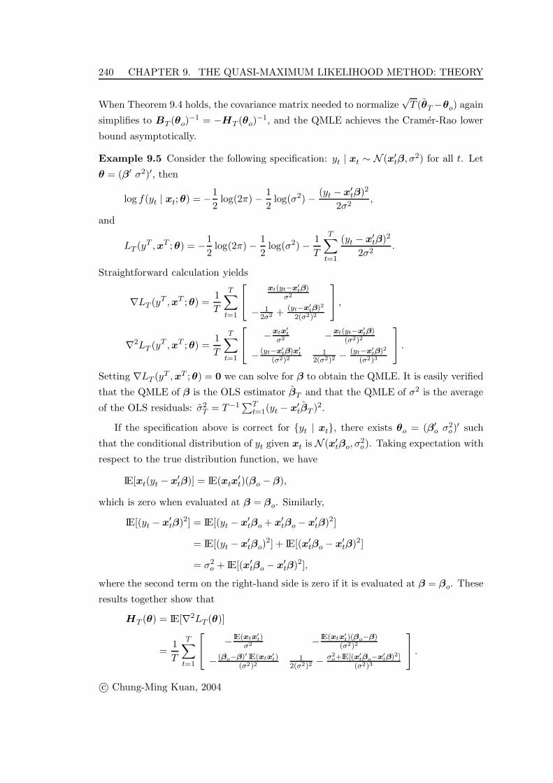
Example 9.5 Consider the following specification: yt | xt ∼ N (x′tβ, σ
2) for all t. Let
θ = (β′ σ2)′, then
log f(yt | xt;θ) = −12
log(2π) − 12
log(σ2) − (yt − x′tβ)2
2σ2,
and
LT (yT ,xT ;θ) = −12
log(2π) − 12
log(σ2) − 1T
T∑t=1
(yt − x′tβ)2
2σ2.
Straightforward calculation yields
∇LT (yT ,xT ;θ) =1T
T∑t=1
⎡⎣ xt(yt−x′tβ)
σ2
− 12σ2 + (yt−x′
tβ)2
2(σ2)2
⎤⎦ ,∇2LT (yT ,xT ;θ) =
1T
T∑t=1
⎡⎣ −xtx′t
σ2 −xt(yt−x′tβ)
(σ2)2
− (yt−x′tβ)x′
t(σ2)2
12(σ2)2 − (yt−x′
tβ)2
(σ2)3
⎤⎦ .Setting ∇LT (yT ,xT ;θ) = 0 we can solve for β to obtain the QMLE. It is easily verified
that the QMLE of β is the OLS estimator βT and that the QMLE of σ2 is the average
of the OLS residuals: σ2T = T−1
∑Tt=1(yt − x′
tβT )2.
If the specification above is correct for yt | xt, there exists θo = (β′o σ
2o)′ such
that the conditional distribution of yt given xt is N (x′tβo, σ
2o). Taking expectation with
respect to the true distribution function, we have
IE[xt(yt − x′tβ)] = IE(xtx
′t)(βo − β),
which is zero when evaluated at β = βo. Similarly,
IE[(yt − x′tβ)2] = IE[(yt − x′
tβo + x′tβo − x′
tβ)2]
= IE[(yt − x′tβo)
2] + IE[(x′tβo − x′
tβ)2]
= σ2o + IE[(x′
tβo − x′tβ)2],
where the second term on the right-hand side is zero if it is evaluated at β = βo. These
results together show that
HT (θ) = IE[∇2LT (θ)]
=1T
T∑t=1
⎡⎣ − IE(xtx′t)
σ2 − IE(xtx′t)(βo−β)
(σ2)2
− (βo−β)′ IE(xtx′t)
(σ2)21
2(σ2)2− σ2
o+IE[(x′tβo−x′
tβ)2](σ2)3
⎤⎦ .c© Chung-Ming Kuan, 2004
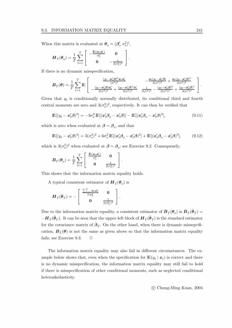
9.3. INFORMATION MATRIX EQUALITY 241
When this matrix is evaluated at θo = (β′o σ
2o)
′,
HT (θo) =1T
T∑t=1
⎡⎣ − IE(xtx′t)
σ2o
0
0 − 12(σ2
o)2
⎤⎦ .If there is no dynamic misspecification,
BT (θ) =1T
T∑t=1
IE
⎡⎣ (yt−x′tβ)2xtx′
t(σ2)2
−xt(yt−x′tβ)
2(σ2)2+ xt(yt−x′
tβ)3
2(σ2)3
− (yt−x′tβ)x′
t2(σ2)2 + (yt−x′
tβ)3x′t
2(σ2)31
4(σ2)2 − (yt−x′tβ)2
2(σ2)3 + (yt−x′tβ)4
4(σ2)4
⎤⎦ .Given that yt is conditionally normally distributed, its conditional third and fourth
central moments are zero and 3(σ2o)
2, respectively. It can then be verified that
IE[(yt − x′tβ)3] = −3σ2
o IE[(x′tβo − x′
tβ)] − IE[(x′tβo − x′
tβ)3], (9.11)
which is zero when evaluated at β = βo, and that
IE[(yt − x′tβ)4] = 3(σ2
o)2 + 6σ2
o IE[(x′tβo − x′
tβ)2] + IE[(x′tβo − x′
tβ)3], (9.12)
which is 3(σ2o)
2 when evaluated at β = βo; see Exercise 9.2. Consequently,
BT (θo) =1T
T∑t=1
⎡⎣ IE(xtx′t)
σ2o
0
0 12(σ2
o)2
⎤⎦ .This shows that the information matrix equality holds.
A typical consistent estimator of HT (θo) is
HT (θT ) = −
⎡⎣ ∑Tt=1 xtx′
t
T σ2T
0
0 12(σ2
T )2
⎤⎦ .Due to the information matrix equality, a consistent estimator of BT (θo) is BT (θT ) =
−HT (θT ). It can be seen that the upper-left block of HT (θT ) is the standard estimator
for the covariance matrix of βT . On the other hand, when there is dynamic missepcifi-
cation, BT (θ) is not the same as given above so that the information matrix equality
fails; see Exercise 9.3.
The information matrix equality may also fail in different circumstances. The ex-
ample below shows that, even when the specification for IE(yt | xt) is correct and there
is no dynamic misspecification, the information matrix equality may still fail to hold
if there is misspecification of other conditional moments, such as neglected conditional
heteroskedasticity.
c© Chung-Ming Kuan, 2004
242 CHAPTER 9. THE QUASI-MAXIMUM LIKELIHOOD METHOD: THEORY
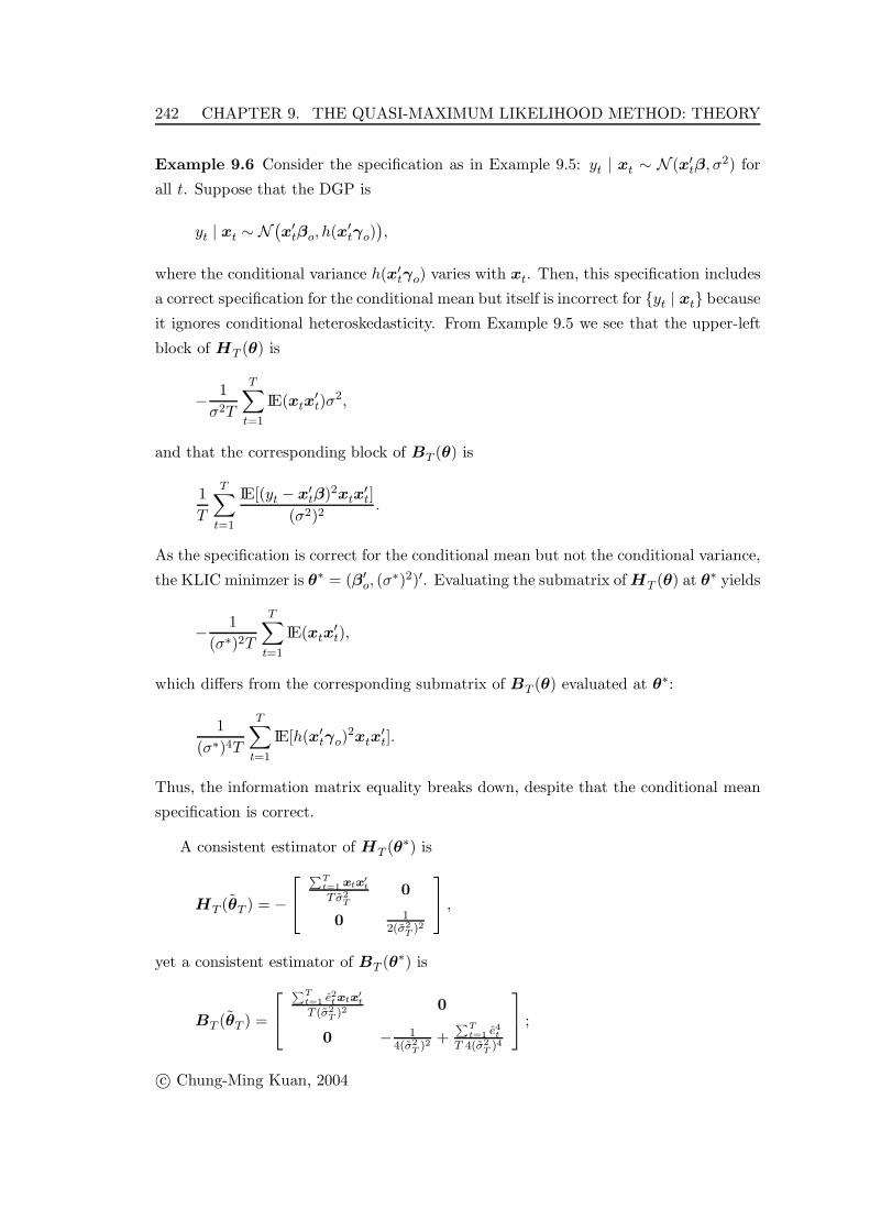
Example 9.6 Consider the specification as in Example 9.5: yt | xt ∼ N (x′tβ, σ
2) for
all t. Suppose that the DGP is
yt | xt ∼ N(x′
tβo, h(x′tγo)),
where the conditional variance h(x′tγo) varies with xt. Then, this specification includes
a correct specification for the conditional mean but itself is incorrect for yt | xt because
it ignores conditional heteroskedasticity. From Example 9.5 we see that the upper-left
block of HT (θ) is
− 1σ2T
T∑t=1
IE(xtx′t)σ
2,
and that the corresponding block of BT (θ) is
1T
T∑t=1
IE[(yt − x′tβ)2xtx
′t]
(σ2)2.
As the specification is correct for the conditional mean but not the conditional variance,
the KLIC minimzer is θ∗ = (β′o, (σ
∗)2)′. Evaluating the submatrix of HT (θ) at θ∗ yields
− 1(σ∗)2T
T∑t=1
IE(xtx′t),
which differs from the corresponding submatrix of BT (θ) evaluated at θ∗:
1(σ∗)4T
T∑t=1
IE[h(x′tγo)
2xtx′t].
Thus, the information matrix equality breaks down, despite that the conditional mean
specification is correct.
A consistent estimator of HT (θ∗) is
HT (θT ) = −
⎡⎣ ∑Tt=1 xtx′
t
T σ2T
0
0 12(σ2
T )2
⎤⎦ ,yet a consistent estimator of BT (θ∗) is
BT (θT ) =
⎡⎣∑T
t=1 e2t xtx′
t
T (σ2T )2
0
0 − 14(σ2
T )2+∑T
t=1 e4t
T 4(σ2T )4
⎤⎦ ;
c© Chung-Ming Kuan, 2004
9.4. HYPOTHESIS TESTING 243
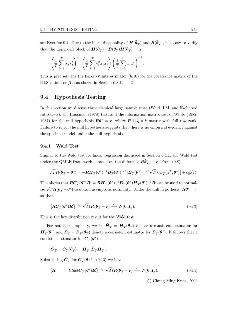
see Exercise 9.4. Due to the block diagonality of H(θT ) and B(θT ), it is easy to verify
that the upper-left block of H(θT )−1B(θT )H(θT )−1 is(1T
T∑t=1
xtx′t
)−1(1T
T∑t=1
e2t xtx′t
)(1T
T∑t=1
xtx′t
)−1
.
This is precisely the the Eicker-White estimator (6.10) for the covariance matrix of the
OLS estimator βT , as shown in Section 6.3.1.
9.4 Hypothesis Testing
In this section we discuss three classical large sample tests (Wald, LM, and likelihood
ratio tests), the Hausman (1978) test, and the information matrix test of White (1982,
1987) for the null hypothesis Rθ∗ = r, where R is q × k matrix with full row rank.
Failure to reject the null hypothesis suggests that there is no empirical evidence against
the specified model under the null hypothesis.
9.4.1 Wald Test
Similar to the Wald test for linear regression discussed in Section 6.4.1, the Wald test
under the QMLE framework is based on the difference RθT ) − r. From (9.8),
√TR(θT − θ∗) = −RHT (θ∗)−1BT (θ∗)1/2
[BT (θ∗)−1/2
√T ∇LT (zT ;θ∗)
]+ oIP(1).
This shows that RCT (θ∗)R′ = RHT (θ∗)−1BT (θ∗)HT (θ∗)−1R′ can be used to normal-
ize√TR(θT −θ∗) to obtain asymptotic normality. Under the null hypothesis, Rθ∗ = r
so that
[RCT (θ∗)R′]−1/2√T (R(θT − r) D−→ N(0, Iq). (9.13)
This is the key distribution result for the Wald test.
For notation simplicity, we let HT = HT (θT ) denote a consistent estimator for
HT (θ∗) and BT = BT (θT ) denote a consistent estimator for BT (θ∗). It follows that a
consistent estimator for CT (θ∗) is
CT = CT (θT ) = H−1T BT H
−1T .
Substituting CT for CT (θ) in (9.13) we have
[R tildebCT (θ∗)R′]−1/2√T (R(θT − r) D−→ N(0, Iq). (9.14)
c© Chung-Ming Kuan, 2004
244 CHAPTER 9. THE QUASI-MAXIMUM LIKELIHOOD METHOD: THEORY
The Wald test statistic is the inner product of the left-hand side of (9.14):
WT = T (RθT − r)′(RCT R′)−1(RθT − r). (9.15)
The limiting distribution of the Wald test now follows from (9.14) and the continuous
mapping theorem.
Theorem 9.7 Suppose that Theorem 9.2 for the QMLE θT holds. Then under the null
hypothesis,
WTD−→ χ2(q),
where WT is defined in (9.15) and q is the number of rows of R.
Example 9.8 Consider the quasi-log-likelihood function specified in Example 9.5. We
write θ = (σ2 β′)′ and β = (b′1 b′2)′, where b1 is (k − s) × 1, and b2 is s × 1. We are
interested in the null hypothesis that b∗2 = Rθ∗ = 0, where R = [0 R1] is s × (k + 1)
and R1 = [0 Is] is s× k. The Wald test can be computed according to (9.15):
WT = T β′2,T (RCT R′)−1β2,T ,
where β2,T = RθT is the estimator of b2.
As shown in Example 9.5, when the information matrix equality holds, CT = −H−1T
is block diagnoal so that
RCT R′ = −RH−1T R′ = σ2
T R1(X′X/T )−1R′
1.
The Wald test then becomes
WT = T β′2,T [R1(X
′X/T )−1R′1]−1β2,T/σ
2T .
In this case, the Wald test is just s times the standard F statistic which is readily
available from most of econometric packages.
9.4.2 Lagrange Multiplier Test
Consider now the problem of maximizing LT (θ) subject to the constraint Rθ = r. The
Lagrangian is
LT (θ) + θ′R′λ,
c© Chung-Ming Kuan, 2004
9.4. HYPOTHESIS TESTING 245
where λ is the vector of Lagrange multipliers. The maximizers of the Lagrangian and
denoted as θT and λT , where θT is the constrained QMLE of θ. Analogous to Sec-
tion 6.4.2, the LM test under the QML framework also checks whether λT is sufficiently
close to zero.
First note that θT and λT satisfy the saddle-point condition:
∇LT (θT ) + R′λT = 0.
The mean-value expansion of ∇LT (θT ) about θ∗ yields
∇LT (θ∗) + ∇2LT (θ†T )(θT − θ∗) + R′λT = 0,
where θ†T is the mean value between θT and θ∗. It has been shown in (9.8) that
√T (θT − θ∗) = −HT (θ∗)−1
√T∇LT (θ∗) + oIP(1).
Hence,
−HT (θ∗)√T (θT − θ∗) + ∇2LT (θ†
T )√T (θT − θ∗) + R′√T λT = oIP(1).
Using the WULLN result: ∇2LT (θ†T ) − HT (θ∗) IP−→ 0, we obtain
√T (θT − θ∗) =
√T (θT − θ∗) − HT (θ∗)−1R′√T λT + oIP(1). (9.16)
This establishes a relationship between the constrained and unconstrained QMLEs.
Pre-multiplying both sides of (9.16) by R and noting that the constrained estimator
θT must satisfy the constraint so that R(θT − θ∗) = 0, we have√T λT = [RHT (θ∗)−1R′]−1R
√T (θT − θ∗) + oIP(1), (9.17)
which relates the Lagrangian multiplier and the unconstrained QMLE θT . When The-
orem 9.2 holds for the normalized θT , we obtain the following asymptotic normality
result for the normalized Lagrangian multiplier:
Λ−1/2T
√T λT = Λ−1/2
T [RHT (θ∗)−1R′]−1R√T (θT − θ∗) D−→ N(0, Iq), (9.18)
where
ΛT (θ∗) = [RHT (θ∗)−1R′]−1RCT (θ∗)R′[RHT (θ∗)−1R′]−1.
Let HT = HT (θT ) denote a consistent estimator for HT (θ∗) and CT = CT (θT ) denote
a consistent estimator for CT (θ∗), both based on the constrained QMLE θT . Then,
ΛT = (RH−1T R′)−1RCT R′(RH
−1T R′)−1
c© Chung-Ming Kuan, 2004
246 CHAPTER 9. THE QUASI-MAXIMUM LIKELIHOOD METHOD: THEORY
is consistent for ΛT (θ∗). It follows from (9.18) that
Λ−1/2T
√T λT = Λ
−1/2T (RH
−1T R′)−1R
√T (θT − θ∗) D−→ N(0, Iq), (9.19)
The LM test statistic is the inner product of the left-hand side of (9.19):
LMT = T λ′T Λ
−1T λT = T λ
′T RH
−1T R′(RCT R′)−1RH
−1T R′λT . (9.20)
The limiting distribution of the LM test now follows easily from (9.19) and the contin-
uous mapping theorem.
Theorem 9.9 Suppose that Theorem 9.2 for the QMLE θT holds. Then under the null
hypothesis,
LMTD−→ χ2(q),
where LMT is defined in (9.20) and q is the number of rows of R.
Remark: When the information matrix equality holds, the LM statistic (9.20) becomes
LMT = −T λ′T RH
−1T R′λT = −T∇LT (θT )′H
−1T ∇LT (θT ),
which mainly involves the averages of scores: ∇LT (θT ). The LM test is thus a test that
checks if the average of scores is sufficiently close to zero and hence also known as the
score test.
Example 9.10 Consider the quasi-log-likelihood function specified in Example 9.5. We
write θ = (σ2 β′)′ and β = (b′1 b′2)′, where b1 is (k − s) × 1, and b2 is s × 1. We are
interested in the null hypothesis that b∗2 = Rθ∗ = 0, where R = [0 R1] is s × (k + 1)
and R1 = [0 Is] is s× k. From the saddle-point condition,
∇LT (θT ) = −RλT .
which can be partitioned as
∇LT (θT ) =
⎡⎢⎢⎢⎣∇σ2LT (θT )
∇b1LT (θT )
∇b2LT (θT )
⎤⎥⎥⎥⎦ =
⎡⎢⎢⎢⎣0
0
−λT
⎤⎥⎥⎥⎦ = −R′λT .
Partitioning xt accordingly as (x′1t x′
2t)′, we have
∇b2LT (θT ) =
1T σ2
T
T∑t=1
x2tεt = X ′2ε/(T σ
2T ).
c© Chung-Ming Kuan, 2004
9.4. HYPOTHESIS TESTING 247
where σ2T = ε′ε/T , and ε is the vector of constrained residuals obtained from regressing
yt on x1t and X2 is the T×s matrix whose t th row is x′2t. The LM test can be computed
according to (9.20):
LMT = T
⎡⎢⎢⎢⎣0
0
X ′2ε/(T σ
2T )
⎤⎥⎥⎥⎦′
H−1T R′(RCT R′)−1RH
−1T
⎡⎢⎢⎢⎣0
0
X ′2ε/(T σ
2T )
⎤⎥⎥⎥⎦ ,which converges in distribution to χ2(s) under the null hypothesis. Note that we do
not have to evaluate the complete score vector for computing the LM test; only the
subvector of the score that corresponds to the constraint matters.
When the information matrix equality holds, the LM statistic has a simpler form:
LMT = T [0′ ε′X2/T ](X ′X/T )−1[0′ ε′X2/T ]′/σ2T
= T [ε′X(X ′X)−1X ′ε/ε′ε]
= TR2,
where R2 is the non-centered coefficient of determination obtained from the auxiliary
regression of the constrained residuals εt on x1t and x2t.
Example 9.11 (Breusch-Pagan) Suppose that the specification is
yt | xt, ζt ∼ N(x′
tβ, h(ζ′tα)),
where h : R → (0,∞) is a differentiable function, and ζ ′tα = α0 +
∑pi=1 ζtiαi. The null
hypothesis is conditional homoskedasticity, i.e., α1 = · · · = αp = 0 so that h(α0) = σ20 .
Breusch and Pagan (1979) derived the LM test for this hypothesis under the assumption
that the information matrix equality holds. This test is now usually referred to as the
Breusch-Pagan test.
Note that the constrained specification is yt | xt, ζt ∼ N (x′tβ, σ
2), where σ2 =
h(α0). This is leads to the standard linear regression model without heteroskedasticity.
The constrained QMLEs for β and σ2 are, respectively, the OLS estimators βT and
σ2T =∑T
t=1 e2t/T , where et are the OLS residuals. The score vector corresponding to α
is:
∇αLT (yt,xt, ζt;θ) =1T
T∑t=1
[h′(ζ ′
tα)ζt
2h(ζ ′tα)
((yt − x′
tβ)2
h(ζ ′tα)
− 1)]
,
c© Chung-Ming Kuan, 2004
248 CHAPTER 9. THE QUASI-MAXIMUM LIKELIHOOD METHOD: THEORY
where h′(η) = dh(η)/ dη. Under the null hypothesis, h′(ζ ′tα
∗) = h′(α∗0) is just a
constant, say, c. The score vector above evaluated at the constrained QMLEs is
∇αLT (yt,xt, ζt; θT ) =c
T
T∑t=1
[ζt
2σ2T
(ε2tσ2
T
− 1)]
.
The (p + 1) × (p + 1) block of the Hessian matrix corresponding to α is
1T
T∑t=1
[−(yt − x′
tβ)2
h3(ζ ′tα)
+1
2h2(ζ ′tα)
][h′(ζ ′α)]2ζtζ
′t
+[(yt − x′
tβ)2
2h2(ζ ′tα)
− 12h2(ζ ′
tα)
]h”(ζ ′α)ζtζ
′t.
Evaluating the expectation of this block at θ∗ = (βo α∗0 0′)′ and noting that (σ∗)2 =
h(α∗0) we have(
c2
2[(σ∗)2]2
)(1T
T∑t=1
IE(ζtζ′t)
),
which, apart from the constant c, can be estimated by(c2
2[σ2T ]2
)(1T
T∑t=1
(ζtζ′t)
).
The LM test is now readily derived from the results above when the information matrix
equality holds.
Setting dt = ε2t/σ2T − 1, the LM statistic is
LMT =
(T∑
t=1
dtζ′t
)(T∑
t=1
ζtζ′t
)−1( T∑t=1
ζtdt
)/2
= d′Z(Z ′Z)−1Z′d/2
D−→ χ2(p),
where d is T×1 with the t th element dt, and Z is the T×(p+1) matrix with the t th row
ζ ′t. It can be seen that the numerator of the LM statistic is the (centered) regression sum
of squares (RSS) of regressing dt on ζt. This shows that the Breusch-Pagan test can also
be computed by running an auxiliary regression and using the resulting RSS/2 as the
statistic. Intuitively, this amounts to checking whether the variables in ζt are capable
of explaining the square of the (standardized) OLS residuals. It is also interesting to
see that the value of c and the functional form of h do not matter in deriving the
c© Chung-Ming Kuan, 2004
9.4. HYPOTHESIS TESTING 249
statistic. The latter feature makes the Breusch-Pagan test a general test for conditional
heteroskedasticity.
Koenker (1981) noted that under conditional normality,∑T
t=1 d2t /T
IP−→ 2. Thus, a
test that is more robust to non-normality and asymptotically equivalent to the Breusch-
Pagan test is to replace the denominator 2 with∑T
t=1 d2t/T . This robust version can be
expressed as
LMT = T [d′Z(Z ′Z)−1Z′d/d′d] = TR2,
where R2 is the (centered) R2 from regressing dt on ζt. This is also equivalent to the
centered R2 from regressing ε2t on ζt.
Remarks:
1. To compute the Breusch-Pagan test, one must specify a vector ζt that determines
the conditional variance. Here, ζt may contain some or all the variables in xt. If
ζt is chosen to include all elements of xt, their squares and pairwise products, the
resulting TR2 is also the White (1980) test for (conditional) heteroskedasticity of
unknown form. The White test can also be interpreted as an “information matrix
test” discussed below.
2. The Breusch-Pagan test is obtained under the condition that the information
matrix equality holds. We have seen that the information matrix equality may
fail when there is dynamic misspecification. Thus, the Breusch-Pagan test is not
valid when, e.g., the errors are serially correlated.
Example 9.12 (Breusch-Godfrey) Given the specification yt | xt ∼ N (x′tβ, σ
2),
suppose that one would like to check if the errors are serially correlated. Consider first
the AR(1) errors: yt −x′tβ = ρ(yt−1 − x′
t−1β) + ut with |ρ| < 1 and ut a white noise.
The null hypothesis is ρ∗ = 0, i.e., no serial correlation. It can be seen that a general
specification that allows for serial correlations is
yt | yt−1,xt,xt−1 ∼ N (x′tβ + ρ(yt−1 − x′
t−1β), σ2u).
The constrained specification is just the standard linear regression model yt = x′tβ.
Testing the null hypothesis that ρ∗ = 0 is thus equivalent to testing whether an ad-
ditional variable yt−1 − xt−1β should be included in the mean specification. In the
light of Example 9.10, if the information matrix equality holds, the LM test can be
computed as TR2, where R2 is obtained from regressing the OLS residuals εt on xt and
c© Chung-Ming Kuan, 2004
250 CHAPTER 9. THE QUASI-MAXIMUM LIKELIHOOD METHOD: THEORY
εt−1 = yt−1 −xt−1βT . This is precisely the Breusch (1978) and Godfrey (1978) test for
AR(1) errors with the limiting χ2(1) distribution.
The test above can be extended straightforwardly to check AR(p) errors. By regress-
ing εt on xt and εt−1, . . . , εt−p, the resulting TR2 is the LM test when the information
matrix equality holds and has a limiting χ2(p) distribution. Such tests are known as
the Breusch-Godfrey test. Moreover, if the specification is yt − x′tβ = ut + αut−1, i.e.,
the errors follow an MA(1) process, we can write
yt | xt, ut−1 ∼ N (x′tβ + αut−1, σ
2u).
The null hypothesis is α∗ = 0. It is readily seen that the resulting LM test is identical
to that for AR(1) errors. Thus, the Breusch-Godfrey test for MA(p) errors is the same
as that for AR(p) errors.
Remarks:
1. The Breusch-Godfrey tests discussed above are obtained under the condition that
the information matrix equality holds. We have seen that the information matrix
equality may fail when, for example, there is neglected conditional heteroskedastic-
ity. Thus, the Breusch-Godfrey tests are not valid when conditional heteroskedas-
ticity is present.
2. It can be shown that the square of Durbin’s h test is also an LM test. While
Durbin’s h test may not be feasible in practice, the Breusch-Godfrey test can
always be computed.
9.4.3 Likelihood Ratio Test
As discussed in Section 6.4.3, the LR test compares the performance of the constrained
and unconstrained specifications based on their likelihood ratio:
LRT = −2T [LT (θT ) − LT (θT )]. (9.21)
Utilizing the relationship between the constrained and unconstrained QMLEs (9.16) and
the relationship between the Lagrangian multiplier and unconstrained QMLE (9.17), we
can write√T (θT − θT ) = HT (θ∗)−1R′√T λT + oIP(1)
= HT (θ∗)−1R′(9.22)
c© Chung-Ming Kuan, 2004
9.4. HYPOTHESIS TESTING 251
By Taylor expansion of LT (θT ) about θT ,
−2T [LT (θT ) − LT (θT )]
= −2T∇LT (θT )(θT − θT ) − T (θT − θT )′HT (θT )(θT − θT ) + oIP(1)
= −T (θT − θT )′HT (θ∗)(θT − θT ) + oIP(1)
= −T (θT − θ∗)′R′[RHT (θ∗)−1R′]−1R(θT − θ∗) + oIP(1),
where the second equality follows because ∇LT (θT ) = 0. It can be seen that the right-
hand side is essentially the Wald statistic when −RHT (θ∗)−1R′ is the normalizing
variance-covariance matrix. This leads to the following distribution result for the LR
test.
Theorem 9.13 Suppose that Theorem 9.2 for the QMLE θT and the information ma-
trix equality both hold. Then under the null hypothesis,
LRTD−→ χ2(q),
where LRT is defined in (9.21) and q is the number of rows of R.
Theorem 9.13 differs from Theorem 9.7 and Theorem 9.9 in that it also requires
the validity of the information matrix equality. When the information matrix equality
does not hold, −RHT (θ∗)−1R′ is not a proper normalizing matrix so that LRT does
not have a limiting χ2 distribution. This result clearly indicates that, when LT is
constructed by specifying density functions for yt | xt, the LR test is not robust to
dynamic misspecification and misspecifications of other conditional attributes, such as
neglected conditional heteroskedasticity. By contrast, the Wald and LM tests can be
made robust by employing a proper normalizing variance-covariance matrix.
c© Chung-Ming Kuan, 2004
252 CHAPTER 9. THE QUASI-MAXIMUM LIKELIHOOD METHOD: THEORY
Exercises
9.1 Let g and f be two density functions. Show that the KLIC II(g :f) does not obey
the triangle inequality, i.e., II(g : f) ≤ II(g : h) + II(h : f) for any other density
function h.
9.2 Prove equations (9.11) and (9.12) in Example 9.5.
9.3 In Example 9.5, suppose there is dynamic misspecification. What is BT (θ∗)?
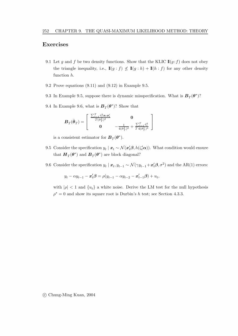
9.4 In Example 9.6, what is BT (θ∗)? Show that
BT (θT ) =
⎡⎣∑T
t=1 e2t xtx′
t
T (σ2T )2
0
0 − 14(σ2
T )2+∑T
t=1 e4t
T 4(σ2T )4
⎤⎦is a consistent estimator for BT (θ∗).
9.5 Consider the specification yt | xt ∼ N (x′tβ, h(ζ
′tα)). What condition would ensure
that HT (θ∗) and BT (θ∗) are block diagonal?
9.6 Consider the specification yt | xt, yt−1 ∼ N (γyt−1+x′tβ, σ
2) and the AR(1) errors:
yt − αyt−1 − x′tβ = ρ(yt−1 − αyt−2 − x′
t−1β) + ut,
with |ρ| < 1 and ut a white noise. Derive the LM test for the null hypothesis
ρ∗ = 0 and show its square root is Durbin’s h test; see Section 4.3.3.
c© Chung-Ming Kuan, 2004
9.4. HYPOTHESIS TESTING 253
References
Amemiya, Takeshi (1985). Advanced Econometrics, Cambridge, MA: Harvard Univer-
sity Press.
Breusch, T. S. (1978). Testing for autocorrelation in dynamic linear models, Australian
Economic Papers, 17, 334–355.
Breusch, T. S. and A. R. Pagan (1979). A simple test for heteroscedasticity and random
coefficient variation, Econometrica, 47, 1287–1294.
Engle, Robert F. (1982). Autoregressive conditional heteroskedasticity with estimates
of the variance of U.K. inflation, Econometrica, 50, 987–1007.
Godfrey, L. G. (1978). Testing against general autoregressive and moving average error
models when the regressors include lagged dependent variables, Econometrica,
46, 1293–1301.
Godfrey, L. G. (1988). Misspecification Tests in Econometrics: The Lagrange Multiplier
Principle and Other Approaches, New York: Cambridge University Press.
Hamilton, James D. (1994). Time Series Analysis, Princeton: Princeton University
Press.
Hausman, Jerry A. (1978). Specification tests in econometrics, Econometrica, 46, 1251–
1272.
Koenker, Roger (1981). A note on studentizing a test for heteroscedasticity, Journal of
Econometrics, 17, 107–112.
White, Halbert (1980). A heteroskedasticity-consistent covariance matrix estimator and
a direct test for heteroskedasticity, Econometrica, 48, 817–838.
White, Halbert (1982). Maximum likelihood estimation of misspecified models, Econo-
metrica, 50, 1–25.
White, Halbert (1994). Estimation, Inference, and Specification Analysis, New York:
Cambridge University Press.
c© Chung-Ming Kuan, 2004