A quality assessment on the DEM matching-based RPC bias ...

Earth Observation and Geomatics Engineering 3(2) (2019) 12–23

__________

* Corresponding author

E-mail addresses: [email protected] (H. Arefi); [email protected], [email protected] (H. Afsharnia) 12

ABSTRACT

Rational polynomial coefficients delivered by satellite image vendors facilitate the geometric processing

of images. However, compensating the inherent bias of these coefficients requires in-situ ground control

collection. Existing global digital elevation models are an alternative for in-situ control data collection. In

this regard, the well-known DEM matching technique can be applied for aligning the image-driven DEMs

with the existing global elevation models. In this study, three image-driven DEMs were generated using a

commercial programming application. The commercial software, similar to the majority of other software

packages, performs epipolar resampling using vendor-provided RPCs before image matching. These

generated DEMs were imported to the DEM matching technique and the estimated matching parameters

were utilized for correcting the bias of RPCs on the ground. We showed that epipolar resampling with

vendor-provided RPCs imposes some geometric distortions to the generated DEMs and therefore,

estimated that DEM matching parameters cannot be employed for RPC bias correction. In two study areas,

while the geopositioning accuracy after bias correction was improved 95.6% and 93.1% using the

commercial software, we achieved 97.8% and 97.4% improvement using the programming.

S KEYWORDS

Satellite stereo images

RPC bias correction

Digital Elevation Models

DEM matching

1. Introduction

High-Resolution Satellite Images (HRSIs) are among the

primary sources of generating digital elevation models. The

spatial resolution of these images ranges between 1m to 5m,

and therefore, each image covers several square kilometers.

HRSIs are supplied with Rational Polynomial Coefficients

(RPCs).

Systematic errors are inherent in the RPCs (Toutin 2004,

Aguilar & Nemmaoui et al. 2019). The complexity of these

errors is different in each satellite. Also, regarding the

acquired image data with a specific satellite, the magnitude

of errors varies and should be corrected. Correction methods

are called bias correction methods (Fraser & Dial et al. 2006)

and may be described by a constant shift or constant shift and

drift, and or by the affine transformation model (Tong & Liu

et al. 2010). The parameters of these models are estimated

using the ground control data.

The most commonly employed control data to estimate the

parameters of the bias correction model are Ground Control

Points (GCPs). In-situ collection of GCPs is a time- and

energy-consuming task (Misra & Moorthi et al. 2015).

Various techniques have been introduced as alternatives to

direct the collection of GCPs.

Bias correction strategy can be designed for a single-image

(Safdarinezhad & Mokhtarzade et al. 2016), the stereo image

pairs (Teo & Huang 2013, Rastogi & Agrawal et al. 2015,

Wu & Tang et al. 2015), or a block of images (d’Angelo &

Reinartz 2012, Oh & Lee et al. 2013). DEM matching was

first proposed by (Ebner & Müller 1986) for block

adjustment of aerial photographs. Then, its complete

mathematical relations were developed based on minimizing

the sum of squares of vertical differences between two

elevation models (Rosenholm & Torlegard 1987).

For generating the 3D stereo models, after conducting the

image matching technique between the stereo image pair, the

webs i t e : h t t ps : / / eoge .u t . ac . i r

A quality assessment on the DEM matching-based RPC bias correction

Hamed Afsharnia1,2, Hossein Arefi1*

1 School of Surveying and Geospatial Engineering, College of Engineering, University of Tehran, Tehran, Iran 2 Department of Surveying Engineering, University of Zanjan, Zanjan, Iran

Article history:

Received: 25 February 2019, Received in revised form: 17 August 2019, Accepted: 4 September 2019

DOI: 10.22059/eoge.2020.286773.1059

mailto:[email protected]



https://eoge.ut.ac.ir/

Afsharnia, Arefi, 2019

13

resulted matched points and vendor-provided RPCs are

imported into the space intersection step. We named these

stereo models as image-driven digital elevation models or

simply as IDEMs.

In (d’Angelo & Schwind et al. 2009), the DEM matching

method was performed on the satellite stereo images without

describing the mathematical model of the matching. Also,

sufficient assessments were not made in order to determine

the efficiency of the method in linear array images. The

complete expansion of the mathematical model of DEM

matching for satellite imagery was performed by (Kim &

Jeong 2010, Kim & Jeong 2011) based on the Rigorous

Sensor Model (RSM).

As a consequence, if there is more than one image, the

freely available global elevation models are applied as the

alternative to the GCPs. These models can also be in the form

of elevation profiles. For instance, (Rastogi & Agrawal et al.

2015) performed bias correction using the ICESat/GLAS

laser profiles. In a similar work, these profiles have been

utilized to improve the quality of 1:50000 map production

from ZY-3 stereo images. An improvement in height

precision from 5m to 3m was reported (Li & Tang et al.

2016).

In the present study, the approach proposed by Ebner and

Müller was utilized to discover the bias of RPCs. Therefore,

the 3D similarity transformation model was solved in the

framework of the UTM coordinate system, and then, it was

applied to the generated IDEMs. We focused on the effect of

the IDEM generation procedure in the estimated parameters

of the transformation model. The most employed pre-

processing step in the IDEM generation algorithms is the

epipolar resampling, generally using the vendor-provided

RPCs (Alidoost & Azizi et al. 2015, Alizadeh Naeini &

Fatemi et al. 2019). We designed a few scenarios to assess

the effect of this big step in the DEM matching procedure.

As a new achievement, we analyzed the results of epipolar

resampling with vendor-provided RPCs in the geometric

quality of generated IDEMs. In this regard, a popular

software (PCI Geomatica) was used to generate two different

IDEMs. Both IDEMs were generated based on the epipolar-

resampled image pairs; one of them was resampled using the

vendor-provided RPCs (PCIDEM) and the other one using

the modified RPCs by GCPs (GCPDEM).

For a better assessment, we generated an IDEM without

the epipolar resampling based on programming (MATDEM)

to show the effect of resampling with biased RPCs in the

results of no-GCP bias correction.

Section 2 introduces the collected materials and utilized

mathematical models. The experimental results are reported

in Section 3 and discussed in Section 4. Finally, the

concluding remarks are presented in Section 5.

2. Materials and Methods

2.1. Study areas and data specifications

Two study areas in Iran were selected for performing the

experiments. Each area consists of a pair of Cartosat-1 stereo

images. The geographic locations of these areas are

presented in Figure 1.

Figure 1. Geographic location of the two study areas

Table 1. Specifications of RDEM and IDEMs

GCPDEM PCIDEM MATDEM SRTM V3 (RDEM) Elevation models

PCI Geomatica

software PCI Geomatica

software Implemented

program

NASA Website (JPL.

2013) Data source

Point cloud Point cloud Point cloud Raster Data format

0.5 arcseconds 0.5 arcseconds 0.5 arcseconds 1 arcsecond Spatial resolution


14

(a) MATDEM-Region-KA (b) MATDEM-Region-TA

Figure 2. Generated IDEMs for two study areas along with the position of GCPs on

each IDEM. MATDEM is an IDEM generated by programming.

The image pairs were captured in 2008 from the Kalkosh

region, located in Kermanshah Province and, in 2016, from

the Tarom region of Zanjan Province, which we labeled them

Region-KA and Region-TA, respectively.

The vendor-provided RPCs, in-situ collected GCPs, and 1-

arcsecond SRTM data were available for both regions.

According to previous studies (Varga & Bašić 2015,

Santillan & Makinano-Santillan 2016), researchers have

identified that the absolute vertical accuracy of SRTM data

is higher than similar global DEMs. We used the SRTM data

as a Reference DEM (RDEM) in the DEM matching step.

In order to discover the amount of bias in the RPCs, three

IDEMs were generated using available input data. The first

IDEM was generated using an implemented code called

MATDEM without epipolar resampling. The generated

IDEMs and the position of GCPs are shown in Figure 2.

The other two IDEMs were generated using the

OrthoEngine module of PCI Geomatica software with and

without the presence of GCPs, which were named GCPDEM

and PCIDEM, respectively. The general specifications of the

IDEMs and RDEM are listed in Table 1.

2.2. Geometric correction of satellite images

The most commonly used model for geometric correction

of satellite images is the Rational Function Model (RFM).

The RFM is written in the form of the ratio of third-order

polynomials. This model is more straightforward than the

RSM as it can be used without knowing orbital parameters

and internal geometry of the sensor (Li & Niu et al. 2009).

The RFM, as well as some other mathematical models,

such as the Direct Linear Transformation (DLT) model and

the 2D affine model, have been proposed as an alternative to

the RSM in most HRSIs. Since the coefficients of RFM in

the form of RPCs are supplied with satellite images, it is the

most widely used model for geometric correction of these

images. The direct form of RFM equations are written as

(Tao & Hu 2001):

1 3

2 4

, , , , ,

, , , ,

n n n n n n

n n

n n n n n n

P h P hL S

P h P h

(1)

(𝐿𝑛, 𝑆𝑛): Normalized image coordinates

𝑃1, … , 𝑃4: Third-order polynomials

(𝜑𝑛, 𝜆𝑛 , ℎ𝑛): Normalized ground coordinates in the geodetic

coordinate system

The general form of third-order polynomials are as

follows:

31 2

1 2 3

3 3 3

1 2 3

0 0 0

, , ; 3; 1: 20 mm m

n n n k n n n

m m m

P h a h m m m k

(2)

𝑎𝑘: Polynomial coefficients

Although the RFM does not address the source of

geometric errors in the image, by using the terrain-

independent method, its accuracy is approximately near to

the RSM (Fraser & Dial et al. 2006, Topan & Oruc et al.

2014). Therefore, RFM is an appropriate alternative to the

RSM (Jannati & Valadan Zoej et al. 2017).

The RPCs are estimated with the terrain-independent

method by fitting the RFM equations to the direction of rays

reconstructed using satellite ephemeris data. Satellite

ephemeris data have some errors, the effect of which is

propagated to the RPCs. Despite the high accuracy of fitting

(Tao & Hu 2001), the lack of ground control information in

the terrain-independent method causes the error of the

ephemeris data to be propagated to the estimated RPCs (Pan

& Tao et al. 2016). For this reason, there is an absolute error

in these coefficients, which usually decreases by using GCPs.

Fortunately, a significant amount of this error is systematic

and it can be modeled (Teo 2011).

2.3. RPC bias correction approach


15

Figure 3. Study flowchart. Note that each IDEM is separately matched to the SRTM.

As mentioned in the introduction section, the first solution

in reducing the bias of RPCs is the use of GCPs. The global

elevation models that cover wide areas can substitute GCPs.

There cannot be a high expectation from alternative methods;

however, by considering applications that do not require high

accuracies, it is reasonable to utilize these alternatives.

After generating an IDEM from a pair of satellite images,

it can be matched with a global elevation model (e.g.,

RDEM). Although RDEMs usually have a low resolution,

the horizontal accuracy of these models is better than that of

IDEMs derived from Cartosat-1 images (Bagheri & Schmitt

et al. 2018). As a result, after matching two elevation models,

a product is achieved with a better spatial resolution

compared to the RDEM and accuracy higher than that of the

IDEM. This process, without the need for GCP collection,

reduces the bias of RPCs on the final product.

The flowchart of the overall progress of this study is

presented in Figure 3. The process starts with the generation

of IDEMs. Then, each IDEM is individually matched to the

RDEM and the transformation parameters are calculated for

each DEM. Finally, the quality of DEM matching is

evaluated using the collected GCPs.

2.3.1 Mathematical model of DEM matching

Various mathematical models for DEM matching have

been used in similar investigations. For example, in

(Sedaghat & Alizadeh Naeini 2018), three different

mathematical models, including the 3D rigid model, the 3D

similarity transformation, and the 3D affine model, were

applied. However, according to (Kim & Jeong 2011), the 3D

similarity transformation is sufficient for the matching of the

elevation models extracted from a pair of linear array satellite

images.

The formation of mathematical equations for matching the

elevation models requires the introduction of data structures

and their coordinate systems. IDEMs in the form of an

irregular point cloud, without a need for gridding and

interpolation, are directly matched to the global DEM with a

regular structure. The essential changes are the use of the

UTM projection system for the point cloud and SRTM data,

as well as the transformation of the SRTM data from EGM96

to WGS84 to unify the height datum of the two elevation

models.

In this study, a DEM matching method was adopted to

solve all the transformation parameters in an iterative process

simultaneously. This method was implemented based on

Ebner's model (Ebner & Müller 1986) which itself is based

on the 3D similarity transformation as follows:

dΩ

dΦ

,

r r rZ o o o

r r r

r ra

Z Z ZV dE dN dZ N Z

E N N

Z Z ZE Z N E d

E E N

Z ZZ E N dm Z E N Z

E N

(3)

(𝐸, 𝑁, 𝑍): UTM coordinates (Easting, Northing, and

ellipsoid height) of the selected point in the point cloud

𝑍𝑟 : Interpolated height from the RDEM

[𝑑𝐸𝑜 , 𝑑𝑁𝑜 , 𝑑𝑍𝑜 , 𝑑𝛺, 𝑑𝛷, 𝑑𝐾, 𝑑𝑚]: Differential values of the

3D similarity transformation parameters used for DEM

matching

𝑛: Number of selected points


16

Due to the large volume of the generated point cloud as

IDEM, some well-distributed points are selected (named as

selected points). The observation equations for selected

points are written based on equation (3) and each point adds

an equation to this observation equation system. Substituting

𝐺𝐸 = 𝜕𝑍𝑟 𝜕𝐸⁄ and 𝐺𝑁 = 𝜕𝑍𝑟 𝜕𝑁⁄ in equation (3), the matrix

form of this equation is expressed as follows:

1

1 1 1 1 1 1 1 1

1

1 1 1 1 1 1 1 1 11

1

n

n n n n n n n n

r

n r

o

o

E N N E E N E N o

E N n N n n E n E n N n n E n N n

Z Z

Z Z

dE

dN

G G N G Z E G Z G N G E Z G E G N dZ

d

dG G N G Z E G Z G N G E Z G E G N

d

dm

(4)

𝐺𝐸 , 𝐺𝑁: Interpolated directional gradients (slopes) from the

RDEM

1,…,n indices: represents the selected point number

After estimating the transformation parameters, these

parameters are applied to all selected points at the end of each

iteration, as follows:

11

1 1

1

j j

o

o

o

E dK d E dE

N dm dK d N dN

Z d d Z dZ

(5)

𝑗: Iteration number of the DEM matching procedure

Directional gradients are computed from RDEM in the

position of selected points. We know that, at the end of each

iteration of DEM matching, the position of all selected points

is updated. Therefore, directional gradients should be

computed in each iteration.

Although the differential values are applied to the IDEM

in each iteration, the total values of these parameters in all

iterations are reported as the final transformation parameters.

As a result, the mathematical model of the RPC bias

compensation in the ground space can be written as:

j j j

o

j j j

o

j j j

o

E mE KN Z E

N KE mN Z N

Z E N mZ Z

(6)

2.4. Generation of MATDEM

In all steps of the MATDEM generation (except in the seed

point generation step to start the precise image matching

process), any corrections to the geometric properties of

stereo images should be avoided. In this way, the bias in the

vendor-provided RPCs is propagated to the generated DEM.

If the corrections are applied, the actual effect of RPC bias in

the final MATDEM could not be discovered adequately. In

summary, no specific geometric corrections should be

performed before DEM matching. For this purpose, an image

matching strategy is first implemented.

2.4.1. Image matching strategy

The desired specifications for IDEM determine the image

matching method. Here, a dense matching method is needed.

The Least-Squares Image Matching (LSM) method, as an

area-based method, has the potential to achieve high

precision and is mainly used for increasing the accuracy of

other matching methods (Sohn & Park et al. 2005). However,

the LSM method has a small pull-in-range and it is possible

to get into the local minima of the correlation function, which

in turn reduces the reliability of the results. Therefore, it is

essential to produce the appropriate seed points located

within the small convergence radius of the LSM. Here, the

seed points were obtained using a coarse matching method

that incorporates the vendor-provided RPCs and SRTM

elevation model in the image matching procedure.

The seed points are extracted using the coarse matching

method. In this regard, a regular grid should be assumed on

the first image, and the grid points are transferred to the

surface of the SRTM model using the RPCs of this image.

Then, the grid points are transferred to the second image

using the RPCs of this image. Finally, we apply a 1D search

using the cross-correlation method for finding the best match

of each grid point. The corresponding points extracted from

the coarse matching method are named as seed points.

After completing the coarse matching, the precise

matching is performed with the LSM method. As mentioned

in the introduction section, the least-squares technique is

considered to improve the position of the seed points. The

mathematical equations of this technique have been

presented in the literature (Gruen 1985, Zhang 2005). The

LSM is performed in the image domain and is based on the

gray levels of image patches (windows) taken from stereo

images. The dimensions of a square patch are considered to

be 35 by 35 pixels based on the auto-correlation function of

the template patch (Afsharnia & Arefi et al. 2017).

2.4.2. Space intersection using RFM

The corresponding points obtained from precise matching,

along with the RPC data of the stereo images are involved in

the generation of MATDEM. The space intersection

equations based on the direct RFM have been mentioned in

numerous references (Tao & Hu 2001, Fraser & Hanley

2003). The output of space intersection is a 3D point cloud

in a ground space named MATDEM.


17

Table 2. The reference ellipsoids and height layers of the experimental data; in the implementation process, all data

should be transformed into a standard coordinate system.

Reference ellipsoid Height datum Item

WGS84 WGS84 ellipsoid IDEMs

WGS84 EGM96 geoid SRTM (RDEM)

WGS84 WGS84 ellipsoid GCPs

WGS84 WGS84 ellipsoid Common frame

2.4.3. Blunder removal

In general, the geometric quality of MATDEM directly

depends on the image matching quality. The remained false

matches in the corresponding points lead to making some

blunders in MATDEM. Therefore, a process was considered

for identifying and eliminating the systematic blunders

mentioned as follows:

I. Determining a threshold for the number of LSM

iterations to eliminate the points in which the

convergence has not been achieved.

II. Increasing the dimensions of the matching window

if the LSM equations are not converged (which

increases the radiometric content of the image

window and consequently the probability of the

convergence).

III. Removing the blunders of the space intersection.

Based on the two criteria, the number of iterations

and the residual values of space intersection, some

of the generated ground points were eliminated.

The predefined threshold for the number of

iterations was 2, and the residuals that were not

consistent with the remaining residuals were

removed. Since the standard deviation of the space

intersection with the vendor-provided RPC data

was small (sigma is about 1.5 pixels), the residual

values far from the mean of the residual vector

(larger than 3*sigma) indicated a false matching in

the previous step.

IV. Generating a temporary DEM from the extracted

point cloud by applying the median filter and

comparing each point with the surface of this

temporary DEM. In this step, the blunders are

identified and eliminated from the point cloud.

3. Experimental results

Different scenarios were considered to discover the errors

inherent in the vendor-provided RPCs of the stereo pair.

These scenarios were designed based on IDEM generation

strategies. For each study area, we generated three different

IDEMs, namely MATDEM, PCIDEM, and GCPDEM. The

introduced DEM matching method in Section 2 was applied

for all of these IDEMs and then, using the control data, we

evaluated the impact of the IDEM generation strategy in the

bias correction procedure.

Each input data is defined in a specific coordinate frame,

which must be transformed into standard frames. The

reference ellipsoids and height layers of these datasets are

given in Table 2. In the last row of the table, the selected

standard frame is introduced.

The conversion of heights from EGM96/EGM2008 to a

WGS84 ellipsoid was easily achieved by considering the

value of geodetic height at each point. The DEM matching

procedure is performed after bringing all data to the standard

reference frame. The convergence graphs of DEM matching

are presented separately in Figures 4 and 5. These graphs

were related to the 3D similarity transformation.

The values of transformation parameters in different

scenarios are presented in Table 3. The larger parameters

indicated more significant errors in the vendor-provided

RPCs.

Table 3. Estimated parameters of DEM matching in different scenarios. MATDEMs were generated by programming, and

PCIDEMs and GCPDEMs were generated using the PCI Geomatica software with and without GCP, respectively.

𝟏 + 𝒎 𝑲 [sec] 𝝓 [sec] 𝜴 [sec] 𝒁𝒐 [m] 𝒀𝒐 [m] 𝑿𝒐 [m] Scenario Dataset

0.9999 -127.4 -138.1 -84.7 13.6 -256.9 152.2 PCIDEM Region-KA

0.9998 -59.2 -72.2 -32.5 12.1 -255.0 166.2 MATDEM

0.9999 -26.4 1.9 -10.7 -3.2 -2.7 0.8 GCPDEM

0.9977 -253.1 -70.0 -87.2 -422.3 -1019.1 71.3 PCIDEM Region-TA

0.9997 -250.2 107.2 61.7 -413.9 -1008.0 3.3 MATDEM

1.0000 -16.7 50.6 47.8 5.3 0.8 -2.4 GCPDEM


18

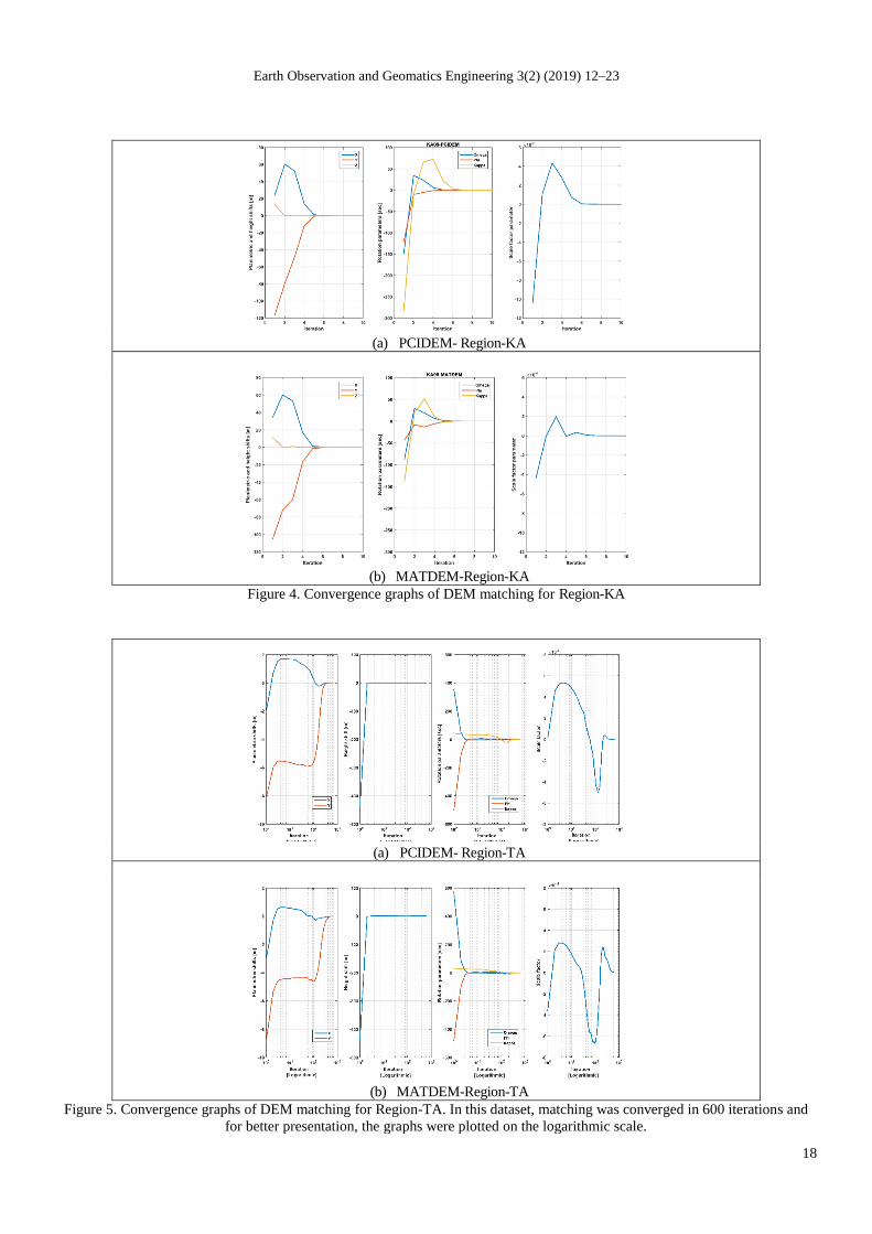
(a) PCIDEM- Region-KA

(b) MATDEM-Region-KA

Figure 4. Convergence graphs of DEM matching for Region-KA

(a) PCIDEM- Region-TA

(b) MATDEM-Region-TA

Figure 5. Convergence graphs of DEM matching for Region-TA. In this dataset, matching was converged in 600 iterations and

for better presentation, the graphs were plotted on the logarithmic scale.


19

3.1. The optimal number of selected points

The available GCPs examined the effect of the number of

selected points in the results of bias correction. We tested

five different sampling rates from the generated dense point

cloud in Region-KA, and then we computed the achieved

horizontal accuracy after bias correction. With the sampling

rate of 1/100, the best accuracy was reached and by

increasing the sampling rate, no further improvements were

observed (as shown in Figure 6). The selected points are

distributed uniformly and randomly.

Figure 6. The horizontal accuracy derived from the

differences between the longitudes and the latitudes of

GCPs and their corresponding bias-corrected points in

Region-KA.

3.2. Quality assessment

The evaluation of DEM matching was carried out in three

ways. One external and two internal evaluations were

considered as follows:

o an external evaluation using GCPs

o visual comparison by generating height difference

maps

o and, statistical analyses using height difference

histograms

3.2.1. Accuracy criteria

If a normal distribution is presumed for the height

difference vector, the following criteria can be presented in

the quality evaluation of DEM matching:

2

1

1

n

iiRMSE Z

n (7)

1

1

n

iiMeanerror Z Z

n (8)

2

1

1 68

1

n

iiStd LE Z Z

n

(9)

∆𝑍𝑖: Height difference between the IDEM and the RDEM at

the point 𝑖

𝑅𝑀𝑆𝐸: RMSE of the ∆𝑍 vector based on the 68% confidence

interval

𝑆𝑡𝑑: Standard deviation of height differences around the

𝑀𝑒𝑎𝑛 𝑒𝑟𝑟𝑜𝑟 based on the 68% confidence interval

In addition, a robust criterion should be created that would

not be sensitive to outlier elements. The Normalized Median

Absolute Deviation (𝑁𝑀𝐴𝐷) is a robust estimator expressed

as follows (Höhle & Höhle 2009):

1.4826 ( )i iNMAD median Z median Z (10)

In the following, the details of each evaluation and

achieved results are presented.

Table 4. Statistical information on the difference between bias-corrected and GPS coordinates

Dataset Item Scenario mean

[m]

|max|

[m]

RMS

[m]

RMS

[pixel]

NMAD

[m]

Region-KA

Longitude PCIDEM -13.0 20.6 14.0 5.6 -

MATDEM 0.2 3.6 2.3 0.9 -

Latitude PCIDEM 4.2 9.4 5.1 2.0 -

MATDEM 6.4 11.5 7.3 2.9 -

Height PCIDEM -0.3 10.2 4.7 - 4.2

MATDEM -1.4 9.1 3.7 - 2.4

Region-TA

Longitude PCIDEM 54.4 73.6 57.0 22.8 -

MATDEM -8.3 33.3 18.6 7.4 -

Latitude PCIDEM 3.1 49.4 38.8 15.5 -

MATDEM 12.9 29.2 17.9 7.2 -

Height PCIDEM -1.4 12.8 10.3 - 10.0

MATDEM -0.9 6.8 3.7 - 1.7


20

3.2.2. The visual comparison

The visual comparison illustrated in Figure 7 shows the

difference maps before and after DEM matching and also

provides a basis for interpretations that cannot be performed

by statistical analysis.

(a) PCIDEM0-Region-KA (b) PCIDEM10-Region-KA

(c) MATDEM0-Region-KA (d) MATDEM10-Region-KA

(e) PCIDEM0-Region-TA (f) PCIDEM600-Region-TA

(g) MATDEM0-Region-TA (h) MATDEM600-Region-TA

Figure 7. Height difference maps between IDEMs and

their corresponding RDEM before and after conducting

the DEM matching step in different scenarios. The

numbers at the end of each IDEM's name show the

number of iterations. MATDEMs were generated by

programming and PCIDEMs were generated using the

PCI Geomatica software.

3.2.3. Histogram analysis

The main objective of DEM matching methods is to reduce

the vertical distance between two DEMs by applying the

suitable geometric transformation. As a result, the histogram

of height differences at the end of iterations could be an

internal criterion for assessing the quality of matching. The

histograms of height differences are shown in Figure 8.

It is not possible to analyze the quality of DEM matching

only by considering the histograms and the height difference

maps. Hence, the horizontal and altimetric control data have

been used for a reliable analysis.

(a) PCIDEM-Region-KA

(b) MATDEM-Region-KA

(c) PCIDEM-Region-TA

(d) MATDEM-Region-TA

Figure 8. Histograms of height differences between

IDEMs and their corresponding RDEM before and after

DEM matching step in different scenarios.

3.3. Accuracy assessment using the GCPs

As mentioned in Section 2, a few GCPs measured by the

differential GPS technique were collected from the study

areas (9 GCPs for Region-KA and 6 GCPs for Region-TA).

In the PCIDEMs, the GCPs were introduced as checkpoints

to the software. In the case of MATDEMs, the RF-derived


21

coordinates of points in the ground space were calculated

using vendor-provided RPCs and the image coordinates of

GCPs. Then, the 3D similarity transformation (estimated

from the DEM matching) was applied to these RF-derived

coordinates to achieve the bias-corrected coordinates.

Finally, we calculated the horizontal and vertical accuracies

by comparing the bias-corrected and in-situ measured

coordinates. These accuracies are presented in Table 4.

As a comparison, we considered two similar types of

research, both of which selected Cartosat-1 stereo images for

evaluating their proposed method of bias correction. In the

first research conducted in region-KA (Alidoost & Azizi et

al. 2015), the epipolar resampling technique was used to have

a robust, dense image matching. After bias correction of

RPCs by SRTM in 9 GCPs, the evaluation showed an

accuracy of -69.4±15.1m and 7.9±9.1m in X (longitude) and

Y (latitude) coordinates, respectively. As seen in Table 4, we

achieved an accuracy of 0.2±2.3m and 6.4±7.3m for these

coordinates. There is a significant difference in RMSE values

of longitude coordinate which can be attributed to epipolar

resampling before DEM generation in their research.

In the second research (Alizadeh Naeini & Fatemi et al.

2019), the IDEMs were generated for two study areas using

the PCI Geomatica software. A proposed 2.5D DEM

matching procedure implemented bias correction with

SRTM DEM, and in the evaluation step, only the vertical

accuracy was assessed using a high-resolution reference

DEM. While we achieved a vertical accuracy of -1.4±3.7m

and -0.9±3.7m for two study areas, they reported 2.0±6.3m

and -5.0±5.7m for their selected study areas. The lower

vertical accuracy of their research could be related to the

epipolar resampling with the vendor-provided RPCs.

4. Discussion

Based on the histograms in Figure 8, the output of the

commercial software (PCIDEM) was better matched to the

RDEM than the output of the implemented program

(MATDEM). This is because the frequency of histogram

around zero is more significant in the PCIDEM case for both

datasets.

Unlike what was observed in histogram analysis, the

horizontal accuracy for PCIDEM and MATDEM cases are

14.9m and 7.6m for the dataset of Region-KA and 69.0m and

18.3m for that of Region-TA, respectively. Also, the vertical

accuracies in PCIDEMs are 4.7m and 10.3m for the datasets

of Region-KA and Region-TA, respectively, while in

MATDEMs it is 3.7m for both datasets. These results mean

that after bias correction, MATDEMs are significantly more

accurate than PCIDEMs.

To explain the reasons for these results, we should consider

IDEM generation procedures in different scenarios. In the

generation of MATDEM, the vendor-provided RPCs were

utilized only at the space intersection. However, in PCIDEM

generation, in addition to space intersection, these RPCs

were used to epipolar resampling of image pairs. Thus, we

can conclude that the bias in the RPCs caused a geometric

distortion in parallax values of the generated epipolar pairs,

and this distortion was also propagated to the generated

PCIDEMs.

By looking at the transformation parameters in Table 3, it

is clear that the transformation parameters differ significantly

in the MATDEM and PCIDEM cases. As a result, it can be

concluded that the low accuracy of PCIDEMs is due to the

epipolar resampling with uncorrected RPCs because epipolar

resampling is a necessary step before DEM generation in the

PCI Geomatica software.

5. Conclusion

In order to modify the bias of vendor-provided RPCs, a

global elevation model was used as an alternative for in-situ

collected GCPs. First, an irregular point cloud was extracted

from the stereo images (IDEM). Each point in the IDEM was

produced using the RFM equations and vendor-provided

RPCs. Therefore, it has the RF-derived coordinates and we

assume that the bias contained in the RPCs was propagated

to the RF-derived coordinates. Then, using the DEM

matching method, we attempted to match this IDEM to a

reference global DEM (RDEM). The estimated

transformation parameters of DEM matching were used for

bias correction of RPCs.

We designed three scenarios to assess the effect of IDEM

generation on bias correction of RPCs and evaluated them on

two study areas. The experiment was performed on two

IDEMs that were generated using the PCI Geomatica

software with and without GCPs (GCPDEM and PCIDEM)

and on a generated IDEM using an implemented program

(MATDEM). After evaluating the results using the control

points and control profiles, it was concluded that MATDEM

achieves more accurate results than PCIDEM. As a reason, it

can be stated that epipolar resampling of stereo image pairs

using vendor-provided RPCs in the PCI Geomatica software

before DEM generation causes some distortion in the depths

extracted from these images. Thus, the transformation

parameters estimated in the DEM matching procedure for

PCIDEM could not be considered for bias correction of

RPCs.

In recent years, the majority of image matching algorithms

used epipolar resampling as a pre-processing step. In this

research, we showed that if the vendor-provided RPCs were

used in the epipolar resampling step, the global elevation

models could not be an alternative for GCPs in bias

correction of the RPCs.

Acknowledgement

We thank the data provider, Iranian national geographic

organization. Special thanks are given to the anonymous

reviewers for their careful reading and helpful suggestions.


22

References

Afsharnia, H., H. Arefi, & M. A. Sharifi (2017). "Optimal

Weight Design Approach for the Geometrically-

Constrained Matching of Satellite Stereo Images."

Remote Sensing 9(9): 965.

Aguilar, M. A., A. Nemmaoui, F. J. Aguilar, & R. Qin

(2019). "Quality assessment of digital surface models

extracted from WorldView-2 and WorldView-3 stereo

pairs over different land covers." GIScience & remote

sensing 56(1): 109-129.

Alidoost, F., A. Azizi, & H. Arefi (2015). "The Rational

Polynomial Coefficients Modification Using Digital

Elevation Models." The International Archives of

Photogrammetry, Remote Sensing and Spatial

Information Sciences 40(1): 47.

Alizadeh Naeini, A., S. B. Fatemi, M. Babadi, S. M. J.

Mirzadeh, & S. Homayouni (2019). "Application of 30-

meter global digital elevation models for compensating

rational polynomial coefficients biases." Geocarto

International: 1-16.

Bagheri, H., M. Schmitt, & X. X. Zhu (2018). "Fusion of

TanDEM-X and Cartosat-1 elevation data supported by

neural network-predicted weight maps." ISPRS journal of

photogrammetry and remote sensing 144: 285-297.

d’Angelo, P., & P. Reinartz (2012). "DSM based orientation

of large stereo satellite image blocks." Int. Arch.

Photogramm. Remote Sens. Spatial Inf. Sci 39(B1): 209-

214.

d’Angelo, P., P. Schwind, T. Krauss, F. Barner, & P. Reinartz

(2009). Automated DSM based georeferencing of

Cartosat-1 stereo scenes. ISPRS Hannover Workshop:

High-Resolution Earth Imaging for Geospatial

Information.

Ebner, H., & F. Müller (1986). "Processing of digital three-

line imagery using a generalized model for combined

point determination." Photogrammetria 41(3): 173-182.

Fraser, C. S., G. Dial, & J. Grodecki (2006). "Sensor

orientation via RPCs." ISPRS journal of Photogrammetry

and Remote Sensing 60(3): 182-194.

Fraser, C. S., & H. B. Hanley (2003). "Bias compensation in

rational functions for IKONOS satellite imagery."

Photogrammetric Engineering & Remote Sensing 69(1):

53-57, 0099-1112.

Gruen, A. (1985). "Adaptive least squares correlation: a

powerful image matching technique." South African

Journal of Photogrammetry, Remote Sensing and

Cartography 14(3): 175-187.

Höhle, J., & M. Höhle (2009). "Accuracy assessment of

digital elevation models by means of robust statistical

methods." ISPRS Journal of Photogrammetry and

Remote Sensing 64(4): 398-406.

Jannati, M., M. J. Valadan Zoej, & M. Mokhtarzade (2017).

"A Knowledge-Based Search Strategy for Optimally

Structuring the Terrain Dependent Rational Function

Models." Remote Sensing 9(4): 345.

JPL., N. (2013). NASA Shuttle Radar Topography Mission

Global 1 arc second.

https://lpdaac.usgs.gov/products/srtmgl1v003/ [Data

set]. N. L. DAAC.

Kim, T., & J. Jeong (2010). "Precise mapping of high

resolution satellite images without ground control

points." International Archives of Photogrammetry,

Remote Sensing and Spatial Information Sciences 38(5).

Kim, T., & J. Jeong (2011). "DEM matching for bias

compensation of rigorous pushbroom sensor models."

ISPRS journal of photogrammetry and remote sensing

66(5): 692-699.

Li, G., X. Tang, X. Gao, H. Wang, & Y. Wang (2016). "ZY‐

3 Block adjustment supported by glas laser altimetry

data." The Photogrammetric Record 31(153): 88-107.

Li, R., X. Niu, C. Liu, B. Wu, & S. Deshpande (2009).

"Impact of imaging geometry on 3D geopositioning

accuracy of stereo IKONOS imagery." Photogrammetric

Engineering & Remote Sensing 75(9): 1119-1125.

Misra, I., S. M. Moorthi, D. Dhar, & R. Ramakrishnan

(2015). "A Unified Software Framework for Automatic

Precise Georeferencing of Large Remote Sensing Image

Archives." Procedia Computer Science 46: 812-819.

Oh, J., C. Lee, & D. C. Seo (2013). "Automated HRSI

georegistration using orthoimage and SRTM: Focusing

KOMPSAT-2 imagery." Computers & geosciences 52:

77-84.

Pan, H., C. Tao, & Z. Zou (2016). "Precise georeferencing

using the rigorous sensor model and rational function

model for ZiYuan-3 strip scenes with minimum control."

ISPRS Journal of Photogrammetry and Remote Sensing

119: 259-266.

Rastogi, G., R. Agrawal, & Ajai (2015). "Bias corrections of

CartoDEM using ICESat-GLAS data in hilly regions."

GIScience & Remote Sensing 52(5): 571-585.

Rosenholm, D., & K. Torlegard (1987). "Three-dimensional

absolute orientation of stereo models using digital

elevation models." Photogrammetric engineering and

remote sensing 54: 1385-1389.

Safdarinezhad, A., M. Mokhtarzade, & M. J. V. Zoej (2016).

"Coregistration of satellite images and airborne lidar data

through the automatic bias reduction of rpcs." IEEE

Journal of Selected Topics in Applied Earth Observation

and Remote Sensing, vol. 1, no. 5.

Santillan, J., & M. Makinano-Santillan (2016). "Vertical

Accuracy Assessment of 30-M Resolution Alos, Aster,

and SRTM Global DEMs over Northeastern Mindanao,

Philippines." International Archives of the

Photogrammetry, Remote Sensing & Spatial Information

Sciences 41.

Sedaghat, A., & A. Alizadeh Naeini (2018). "DEM

orientation based on local feature correspondence with


23

global DEMs." GIScience & Remote Sensing 55(1): 110-

129.

Sohn, H. G., C. H. Park, & H. Chang (2005). "Rational

function model‐ based image matching for digital

elevation models." The Photogrammetric Record

20(112): 366-383.

Tao, C. V., & Y. Hu (2001). "A comprehensive study of the

rational function model for photogrammetric

processing." Photogrammetric engineering and remote

sensing 67(12): 0099-1112.

Teo, T.-A. (2011). "Bias compensation in a rigorous sensor

model and rational function model for high-resolution

satellite images." Photogrammetric Engineering &

Remote Sensing 77(12): 1211-1220.

Teo, T.-A., & S.-H. Huang (2013). "Automatic co-

registration of optical satellite images and airborne

LiDAR data using relative and absolute orientations."

IEEE Journal of Selected Topics in Applied Earth

Observations and Remote Sensing 6(5): 2229-2237.

Tong, X., S. Liu, & Q. Weng (2010). "Bias-corrected rational

polynomial coefficients for high accuracy geo-

positioning of QuickBird stereo imagery." ISPRS Journal

of Photogrammetry and Remote Sensing 65(2): 218-226.

Topan, H., M. Oruc, T. Taskanat, & A. Cam (2014).

"Combined efficiency of RPC and DEM accuracy on

georeferencing accuracy of orthoimage: Case study with

Pléiades panchromatic mono image." IEEE Geoscience

and Remote Sensing Letters 11(6): 1148-1152.

Toutin, T. (2004). "Geometric processing of remote sensing

images: models, algorithms and methods." International

journal of remote sensing 25(10): 1893-1924.

Varga, M., & T. Bašić (2015). "Accuracy validation and

comparison of global digital elevation models over

Croatia." International journal of remote sensing 36(1):

170-189.

Wu, B., S. Tang, Q. Zhu, K.-y. Tong, H. Hu, & G. Li (2015).

"Geometric integration of high-resolution satellite

imagery and airborne LiDAR data for improved

geopositioning accuracy in metropolitan areas." ISPRS

Journal of Photogrammetry and Remote Sensing 109:

139-151.

Zhang, L. (2005). "Automatic digital surface model (DSM)

generation from linear array images." Ph.D Dissertation,

Mitteilungen- Institut fur Geodasie und Photogrammetrie

an der Eidgenossischen Technischen Hochschule Zurich:

0252-9335.

A quality assessment on the DEM matching-based RPC bias ...

Documents

Transcript of A quality assessment on the DEM matching-based RPC bias ...