A Probabilistic Treatment of Phylogeny and Sequence Alignment

G.J. Mitchison

The Laboratory of Molecular Biology, Hills Road, Cambridge CB2 2QH, UK

Received: 25 May 1998 / Accepted: 8 December 1998

Abstract. Carrying out simultaneous tree-building andalignment of sequence data is a difficult computationaltask, and the methods currently available are either lim-ited to a few sequences or restricted to highly simplifiedmodels of alignment and phylogeny. A method is givenhere for overcoming these limitations by Bayesian sam-pling of trees and alignments simultaneously. Themethod uses a standard substitution matrix model forresidues together with a hidden Markov model structurethat allows affine gap penalties. It escapes the heavycomputational burdens of other models by using an ap-proximation called the “*” rule, which replaces missingdata by a sum over all possible values of variables. Thebehavior of the model is demonstrated on test sets ofglobins.

Key words: Phylogeny — Alignment — HiddenMarkov model — Tree-HMM — Affine gap penalty —Bayesian sampling

Introduction

Phylogeny and alignment are intimately linked. Whenprotein or nucleotide sequences are used to construct atree, there is an implicit assumption that aligned residuesare evolutionarily derived from a common ancestral resi-due. An error of alignment will introduce noise that canlead to an incorrect tree. Such errors are particularly

likely when remote sequences are aligned by automaticsequence-based methods. Structural alignment can pro-vide a more secure guide when sequences have divergedtoo far to be aligned by sequence alone, but it also failswhen sequences are too remote, for then substantialshifts in the structure can occur.

This is the negative aspect of alignment. A more posi-tive message comes from looking at the informationpresent in insertions and deletions. Kinship may be re-vealed by a shared pattern of gaps, even when sequenceshave diverged considerably. One of the aims of this pa-per is to provide a probabilistic model that allows thiskind of alignment information to be used and combinedwith the more standard information from residues.

Instead of regarding alignment as a preparatory stepfor phylogeny, one can reverse the order of inferencesand take account of phylogeny in carrying out an align-ment. It is reasonable to expect an influence of phylog-eny on alignment. For example, an alignment that im-plies many substitutions between closely relatedsequences is clearly less good than one that makes mostof its changes over large evolutionary distances. Theprobabilistic modeling technique described in this paperallows phylogeny to be taken account of in alignment,and we shall see that different choices of tree can have aconsiderable effect on the type of alignments one gets.

The most ambitious project is to carry out alignmentand phylogeny simultaneously. There have been severalstabs at this problem. Sankoff and Cedergren (1983)gave an algorithm for finding optimal alignments using ascore derived from a tree. Their score is computed by theparsimony method from a tree at each point in ann-dimensional dynamic programming matrix, wheren isthe number of sequences. This method becomes veryCorrespondence to:G.J. Mitchison;e-mail: gjm@mrc-lmb.cam.ac.uk

J Mol Evol (1999) 49:11–22

© Springer-Verlag New York Inc. 1999

unwieldy for more than a small number of sequences;an early proposal for overcoming this problem was tobuild a tree from smaller subtrees (Sankoff et al. 1973),though optimality can then not be guaranteed. Hein(1989) developed an ingenious parsimony-based algo-rithm that is computationally effective for many se-quences. It also treats gaps more realistically thanSankoff and Cedergren’s algorithm, using an affine pen-alty (of the forma + kb for gap lengthk, wherea andbare constants) rather than a simple fixed penalty for sub-stituting a residue by a gap. However, his method is notprobabilistic [though it can be regarded as an approxi-mation to a maximum-likelihood method (Durbin et al.1998)].

Another combined alignment and phylogeny method,the minimum-message length approach of Allison et al.(1992a, b), can readily be interpreted as a probabilisticmodel, producing a maximum-likelihood alignment andtree. The alignment model can be made increasinglycomplex by increasing the size of the automaton thatcreates the message. For instance, an automaton with onestate corresponds to a simple substitution model of gaps,whereas one with three states can model an affine pen-alty. Only for the automaton with one state, however, isthere an algorithm that is computationally tractable.

Finally, there are probabilistic models based on ex-plicit evolutionary substitution and gap-making events(Bishop and Thompson 1986; Thorne et al. 1991, 1992).These enable one to compute the probability of a givenalignment arising over some time period. Such a modelcould in principle be extended to trees, and would thengive an account of phylogeny and alignment founded onthe statistics of individual evolutionary events. However,the treatment so far has been confined to alignments ofonly two sequences and has also used restrictive modelsof gap formation.

It is therefore still an open problem to find a proba-bilistic treatment of alignment and phylogeny which al-lows an adequate modeling of gaps. We suggest an ap-proach that uses sampling on both trees and alignments.Sampling methods are attractive because they give infor-mation about the whole posterior distribution (in thiscase, the distribution of alignments and phylogenetic treeparameters), whereas maximum-likelihood inferencescan lead to biased and unrepresentative answers in high-dimensional spaces. Bayesian sampling has been usedwith considerable success to evaluate alignments of pairsof sequences and to search for distant relatives in a da-tabase (Zhu et al. 1997).

Modeling of Phylogeny and Alignment:The Tree-HMM

Alignment and phylogeny can be treated simultaneouslyby combining an alignment model, a profile-HMM

(Krogh et al. 1994), with a probabilistic model of phy-logeny (Neyman 1971; Felsenstein 1981). The resultingmodel is called a tree-HMM (Mitchison and Durbin1995). The description given here is different from thatin the original paper, stressing the idea of evolutionarychanges of paths through an HMM. This turns out todefine an equivalent model, but the path viewpoint givesmore insight.

The basic idea of a tree-HMM is that a path throughan HMM, which represents an alignment of a sequence,can change as a result of evolution and that the probabil-ity of such changes is given by substitution probabilities.We shall see later that this model is underpinned by anevolutionary process consisting of substitution of resi-dues and insertion–deletion events. With the tree-HMM,we are no longer concerned with emission and transitionprobabilities, as in a standard HMM, but with the prob-abilities of an emission or transition beingsubstitutedbyanother emission or transition. Substitution probabilitiesare, of course, what underlie probabilistic phylogeny,and it is the marriage of these with a hidden Markovstructure which achieves the fusion of phylogeny andalignment.

The HMM in question can have any architecture.Here a profile-HMM structure is assumed, with onlymatch and delete states (Fig. 1), as there are certain com-plications in the use of the insert states (Mitchison andDurbin 1995) present in the original profile-HMM ofKrogh et al. (1994). Insertions are still allowed, however,even though they are not represented by a special state;they occur when a sequence uses a match state at aposition where its ancestor uses a delete state.

Consider now the simplest possible evolutionary tree,T,consisting of a single edge of lengthd,with a leaf nodeat one end and a root node at the other. Let the sequenceof the leaf bex and that at the rooty. The tree signifiesthat x has evolved fromy over an evolutionary distanced. The sequences take paths through the model; Fig. 2shows an example of what these paths might look like fora model of length 4.

Observe that the paths can differ in two ways: theycan use different transitions and states, and they can emitdifferent residues (we include emissions in the definitionof a “path”). To each such difference we assign a prob-ability; multiplying all these individual probabilities thengivesP(x|y,T). The probability of the sequences is then

Fig. 1. An HMM-profile architecture that provides a convenientstructure for a tree-HMM. It is simpler than the standard version, hav-ing no insert states.

12

given byP(x,y|T) 4 P(y|T)P(x|y,T), whereP(y|T) is theprior probability for the root sequence.

Consider now the various types of differences be-tween paths. At the M state at position 1,x emits anA,whereasy emits aV. We assign a probabilityPd(A|V) tothis substitution and assume henceforth that this is thefamiliar Dayhoff matrix element for a distance ofdPAMs (Dayhoff et al. 1978). At position 1 there is a treeT with a V at the root and anA at the leaf. This canbe regarded as a standard (albeit very simple) exampleof phylogeny of residues. We haveP(A,V|T) 4r(V)Pd(A|V), wherer is the prior for emissions. We callthis the “emission tree” at position 1 in the model, andP(A,V|T) will be one of the terms whose product definesP(x,y|T).

In going from position 1 to position 2,y undergoes atransition from state M to M, whereasx undergoes atransition from M to D. We use the compact notation“MM” for the former transition and “MD” for the latter.The substitution of MM by MD can be treated in ananalogous way to substitution of emitted residues, itsprobability being denotedPd(MD|MM). The four pos-sible substitutions form a family of 2 × 2 matrices

SPd~MM|MM!Pd~MM|MD!

Pd~MD|MM!Pd~MD|MD!D (1)

for any value ofd $ 0. We call this thematch-transitionmatrix family. Putting MM at the root ofT and MD at itsleaf defines the match-transition tree at position 1. TheprobabilityP(MD,MM|T), which provides another factorin P(x,y|T), is r(MM)Pd(MD|MM), wherer(MM) is theprior probability for MM.

There are analogous substitution probabilities for thedelete state. Thus at position 3,x undergoes a DM tran−sition andy a DD. The appropriatedelete-transitionprob-ability here,P(DM,DD|T), is given byr(DD)Pd(DM|DD).

Both sequences use the M state at position 1 and bothuse the D state at position 3, but in positions 2 and 4 ofthe model they use different states, andx cannot be re-garded as evolving fromy by a substitution of either amatch-transition or a delete-transition. Instead, one se-quence makes an insertion or deletion relative to theother at positions 2 and 4, and we postulate that theiremissions or transitions in the course of the separatepaths they follow should be treated as independent ofeach other. As an attempt to capture this, we adopt the

Fig. 2. A short tree-HMM for thesimple tree with two nodes shownabove. Two sequences,x andy,corresponding to the leaf node andthe root node are shown, togetherwith the emission and transitiontrees they imply. Note that there isonly a match-transition tree at theBEGIN state because it is treated asa dummy match state that emits noresidue.

13

formal rule of replacing the missing ancestral or descen-dent sequences at such positions by a sum over all pos-sible emissions or transitions, and use the symbol * todenote this sum.

At position 2, for instance, the foregoing rule meansthat the delete-transition tree has DD at the leaf and a *at the root, so

P~DD,* |T! = r~DM!Pd~DD|DM! + r~DD!Pd~DD|DD!

= r~DD!~Pd~DD|DD! + Pd~DM|DD!!

= r~DD! (2)

where the second step assumes that the delete-transitionmatrices form a reversible family. Thus one gets the priorfor DD. Similarly, the match-transition tree at position 2has a * at theleaf and MD at the root, so

P~*, MD|T! = r~MD!Pd~MM|MD! + r~MD!Pd~MD|MD!

= r~MD! (3)

giving the prior probability ofy’s transition MD. Finally,note that at positions where a state is not used by anysequence, for instance, the D at position 1, the tree has*’s at both leaf and root, and the probabilityP(*,*|T)is 1.

Multiplying together the probabilities of all transitionsand emissions in the pathsx, ygivesP(x,y|T). To expressthis formally, let Mk(xi) denote the transition from thematch state used by sequencexi at positionk, or a * if xi

does not use M at positionk. Similarly, let Ek (xi) be theemission, andDk(xi) the transition from the delete state,atk, either being a * if therelevant state is not used. Thenwe have

P~x,y|T! = )k

P~Mk~x!,Mk~y!|T! × P~Dk~x!,Dk~y!|T!

× P~Ek~x!,Ek~y!|T!(4)

Since the root sequencey is generally unknown, to getthe probability of the observed sequence, namely,P(x|T),we must sum over ally. This means summing over allpossible paths, including all possible emissions, fory.Now it is easy to see that this implies

P~x|T! = )k

P~Mk~x!|T!P~Dk~x!|T!P~Ek~x!|T! (5)

whereP(Ek(x)|T) is the probability for the observed emis-sion at positionk obtained by summing over all possibleroot residues, i.e., emissions ofy, and P(Mk(x)|T) andP(Dk(x)|T) are similarly defined by summing over allroot values of the relevant transitions. Equation (4) im-plies Eq. (5) because the sums over possible states andemissions ofy distribute over the product. The * rulemeans that, wheny uses anM state, all transitions from

D are summed over, so all combinations of the terms in(5) occur.

This defines a tree-HMM for the simplest possibletree consisting of a single edge. The definitions extendreadily to any treeT with n leaves (see Fig. 3). Label thenodesi 4 1, . . . , 2n − 1, with i 4 1, . . . ,n the leavesand 2n − 1 the root. Letdi be the length of the edge thathas nodei at the bottom, and leta(i) denote the numberof the node at the top of that edge. Suppose that the leafsequences arex1, x2, . . . , xn and the sequences at ances-tral nodes areyn+1, yn+2, . . . , y2n−1. For a tree of typeLat positionk, whereL 4 E, M, or D, the probability ofthe specific assignments to all its nodes is given by

P~Lk~x1!, . . . ,Lk~xn!,Lk~yn+1!, . . . ,Lk~y2n−1!|T! =

r~Lk~y2n−1!!)i=1

n

Pdi~Lk~xi!|L

k~ya~i!!! )i=n+1

2n−2

Pdi~Lk~yi!|L

k~ya~i!!!

the product being taken over all edges. The analogue of(4) is then

P~x1, . . . ,xn, yn+1, . . . ,y2n−1|T! =

)L)

k

P ~Lk~x1!, . . . ,Lk~xn!, Lk~yn+1!, . . . ,Lk~y2n−1!|T!

and, as before, the sum over all nonleaf nodes, i.e., overall yi, distributes over the product, giving

P~x1, . . . ,xn|T! = )L)

k

P~Lk~x1!, . . . ,Lk~xn!|T!

(6)

In the original paper (Mitchison and Durbin 1995), Eq.(6) was given as thedefinition of the tree-HMM prob-ability, whereas here it is derived from the concept ofsubstitution of paths, using the * rule.

The Phylogenetic Information in Insertionsand Deletions

A similarity in the pattern of insertions and deletions ofa pair of sequences in an alignment may indicate a phy-logenetic relationship. We can use the tree-HMM to as-sess whether this phylogenetic information is significant.

Suppose we are given an alignment of a set of se-quences; this alignment might be determined by struc-ture, for instance. The existence of a fixed alignmentmeans that the path through the tree-HMM for each se-quence is fixed; the tree parametersT and {di} can thenbe varied to maximize the likelihood or sample from theposterior. The substitution probabilities for emissionsconstitute the standard Neyman/Felsenstein model; thesubstitution probabilities for transitions contribute extraterms which derive from the insertions and deletions inthe alignment. The extent to which the log-likelihood ofthe maximum-likelihood topology exceeds that for the

14

next-best topology can be regarded as a measure of dis-crimination of the best topology. By comparing how thisdiscrimination differs with and without the transitionsubstitution probabilities, we can judge whether there isuseful information in insertions and deletions.

We illustrate this with a number of data sets, eachconsisting of four globin sequences. These were pickedfrom a structure-based alignment by the criterion thatthere should be two pairs more closely related withineach pair than between the pairs. The measure of close-ness of sequencesx, y was the maximum-likelihood dis-tance (Felsenstein 1996), defined by

d~x,y! = argmaxd )

iLj

Pd~xi|yj! (7)

where, as usual,Pd(xi|yj) denotes the PAM substitutionprobability, andi L j means thati is aligned toj. Wethen picked sequencesx1, x2, x3, andx4 such thatd(x1,x2)< 300, d(x3,x4) < 300, d(x1,x3) > 300, d(x1,x4) > 300,d(x2,x3) > 300, andd(x2,x4) > 300 PAM units. The meandistance between close pairs (e.g.,x1, x2) was 176 PAM

units, and that between distant pairs (e.g.,x1, x3) was 331PAM units; the corresponding percentage identities ofresidues were 43 and 20%. This method of choosingquadruples has the effect of making one of the threepossible tree topologies more likely than the other two.

To define the tree-HMM used for these data sets, weneed to specify the substitution matrix families and thepriors. The PAM family was used for substitution ofemissions and its equilibrium probabilities for large val-ues of d were used as the emission prior. The match-transition matrix was assumed to have the followingform:

MM MDMM

MDSa + ~1 − a!e−rd ~1 − a!~1 − e−rd!

a − ae−rd 1 − a + ae−rd D (8)

whered is the evolutionary distance,r $ 0 a rate con-stant, and 0# a # 1 determines the equilibrium prob-abilities for larged. If one takes the priors to be theequilibrium probabilities, one getsr(MM) 4 a, r(MD)

Fig. 3. The first few states of a tree-HMM for a treewith five leaves. Unlike Fig. 2, which showed aparticular choice of ancestral sequence, these sequencesare here assumed to be summed over. So only the fiveleaf sequences are shown. These emit the residuesindicated in the alignmentbelow.To compute theprobabilities of data conditioned on the trees, thestandard Neyman/Felsenstein algorithm (post-ordertraversal) is used, with the additional rule that allpossible residues are summed over at a leaf with a *.

15

4 1 − a. This matrix family is reversible and multipli-cative (Durbin et al. 1998) and is convenient because itrequires only two constants,a and r, to be determined.These can be estimated by maximum-likelihood from agiven data set, choosinga andr to maximize the productof all substitution probabilities arising in the data set. Thedelete-transition matrix was assumed to have a similarform, though it was not constrained to have the sameparameters as the match-transition matrix. Table 1 showsvalues of parameters that were obtained by maximum-likelihood estimation from the first 50 protein families inthe database Pfam (Sonnhammer et al. 1997).

For each quadruple, letLi denote the log-likelihoodsfor the three tree topologiesi 4 0,1,2. IfL0 is the largestof these, let

DL 4 min(L0 − L1, L0 − L2) (9)

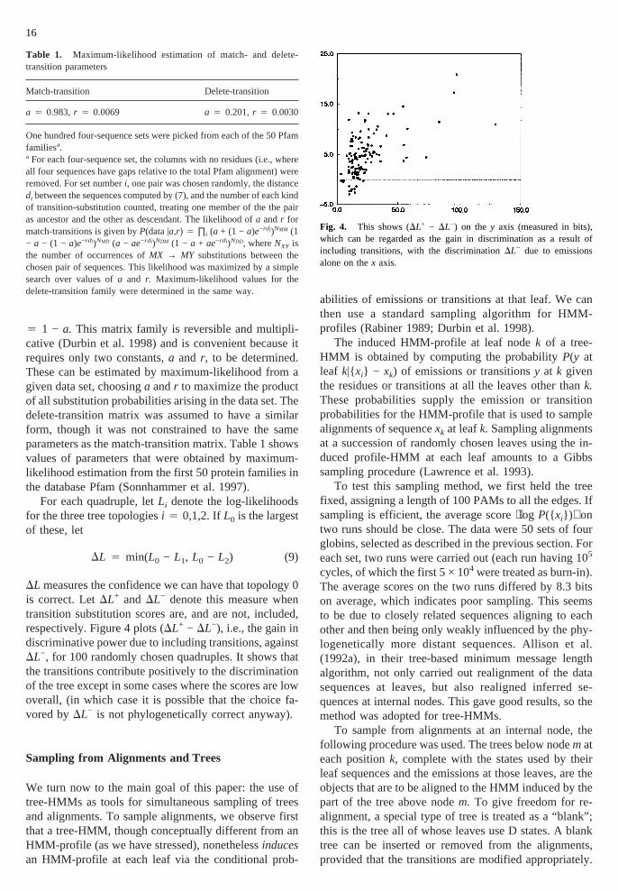
DL measures the confidence we can have that topology 0is correct. LetDL+ and DL− denote this measure whentransition substitution scores are, and are not, included,respectively. Figure 4 plots (DL+ − DL−), i.e., the gain indiscriminative power due to including transitions, againstDL−, for 100 randomly chosen quadruples. It shows thatthe transitions contribute positively to the discriminationof the tree except in some cases where the scores are lowoverall, (in which case it is possible that the choice fa-vored byDL− is not phylogenetically correct anyway).

Sampling from Alignments and Trees

We turn now to the main goal of this paper: the use oftree-HMMs as tools for simultaneous sampling of treesand alignments. To sample alignments, we observe firstthat a tree-HMM, though conceptually different from anHMM-profile (as we have stressed), nonethelessinducesan HMM-profile at each leaf via the conditional prob-

abilities of emissions or transitions at that leaf. We canthen use a standard sampling algorithm for HMM-profiles (Rabiner 1989; Durbin et al. 1998).

The induced HMM-profile at leaf nodek of a tree-HMM is obtained by computing the probabilityP(y atleaf k|{xi} − xk) of emissions or transitionsy at k giventhe residues or transitions at all the leaves other thank.These probabilities supply the emission or transitionprobabilities for the HMM-profile that is used to samplealignments of sequencexk at leafk. Sampling alignmentsat a succession of randomly chosen leaves using the in-duced profile-HMM at each leaf amounts to a Gibbssampling procedure (Lawrence et al. 1993).

To test this sampling method, we first held the treefixed, assigning a length of 100 PAMs to all the edges. Ifsampling is efficient, the average score⟨log P({ xi}) ⟩ ontwo runs should be close. The data were 50 sets of fourglobins, selected as described in the previous section. Foreach set, two runs were carried out (each run having 105

cycles, of which the first 5 × 104 were treated as burn-in).The average scores on the two runs differed by 8.3 bitson average, which indicates poor sampling. This seemsto be due to closely related sequences aligning to eachother and then being only weakly influenced by the phy-logenetically more distant sequences. Allison et al.(1992a), in their tree-based minimum message lengthalgorithm, not only carried out realignment of the datasequences at leaves, but also realigned inferred se-quences at internal nodes. This gave good results, so themethod was adopted for tree-HMMs.

To sample from alignments at an internal node, thefollowing procedure was used. The trees below nodemateach positionk, complete with the states used by theirleaf sequences and the emissions at those leaves, are theobjects that are to be aligned to the HMM induced by thepart of the tree above nodem. To give freedom for re-alignment, a special type of tree is treated as a “blank”;this is the tree all of whose leaves use D states. A blanktree can be inserted or removed from the alignments,provided that the transitions are modified appropriately.

Table 1. Maximum-likelihood estimation of match- and delete-transition parameters

Match-transition Delete-transition

a 4 0.983,r 4 0.0069 a 4 0.201,r 4 0.0030

One hundred four-sequence sets were picked from each of the 50 Pfamfamiliesa.a For each four-sequence set, the columns with no residues (i.e., whereall four sequences have gaps relative to the total Pfam alignment) wereremoved. For set numberi, one pair was chosen randomly, the distancedi between the sequences computed by (7), and the number of each kindof transition-substitution counted, treating one member of the the pairas ancestor and the other as descendant. The likelihood ofa andr formatch-transitions is given byP(data |a,r) 4 ∏i (a + (1 − a)e−rdi)NMM (1− a − (1 − a)e−rdi)NMD (a − ae−rdi)NDM (1 − a + ae−rdi)NDD, whereNXY isthe number of occurrences ofMX → MY substitutions between thechosen pair of sequences. This likelihood was maximized by a simplesearch over values ofa and r. Maximum-likelihood values for thedelete-transition family were determined in the same way.

Fig. 4. This shows (DL+ − DL−) on they axis (measured in bits),which can be regarded as the gain in discrimination as a result ofincluding transitions, with the discriminationDL− due to emissionsalone on thex axis.

16

For instance, if a leaf sequence usesM at positionsk andk + 1, so it makes anMM transition atk, inserting a blanktree at positionk + 1 means that the leaf usesM at k, Dat k + 1, andM at k + 2; hence the leaf sequence makesan MD transition atk and aDM transition atk + 1.

Standard algorithms (Felsenstein 1981; Mitchison andDurbin 1995) enable one to compute the probabilityp↓(y) of emissions or transitions in the tree belowmgiven y at nodem, i.e.,

p↓(y) 4 P({ Lk(xui)} ui below m|y at nodem, T)

Similarly, one can compute the probability ofy at nodemgiven the tree abovem, i.e.,

p↑(y) 4 P(y at nodem|{Lk(xui)} ui abovem, T)

Summing over the product of these distributions gives

(y

p↑~y!p↓~y! =P~$Lk~xi!%|T!

P~$Lk~xui!%ui abovem|T!

(10)

using the fact that the sequences above and belowm areindependent. If we are aligning the part of the tree belownode m to the rest of the tree,P({ Lk(xui

)} ui above m|T)remains fixed, and this constant factor has no effect onthe sampling. With the distinction that the probability isevaluated by the sum in (10), and that the blank treereplaces the use of the D state, the sampling procedure isidentical to that for the leaves. When sampling at internalnodes was included, the difference in average scores ontwo runs fell from 8.3 to 0.6 bits, indicating greatly im-proved sampling. The average scores were also 9.2 bitslarger.

Next we asked whether there was any influence of thetree parameters on the statistics of alignments. Withoutthis, sampling of trees would be pointless, of course. Weused sets of four globins again and looked at two sets oftree distances. The first (Fig. 5, top left) assigns shortdistances to the terminal branches to the leaves and along distance to the connecting branch; the other (Fig. 5,top right) reverses this pattern. Letda denote the averagedistance defined by (7) between sequences on adjacentbranches in the tree, and letdo denote the average dis-tance for sequences that are separated by the internalbranch. We would expect the average value of the ratiodo/da to be larger for a tree with a long internal branchcompared to one with a short internal branch. Figure 5shows that this is what happened. Furthermore, the sameratio, but with percentage identities of residues in placeof distances, was smaller for the tree with a long internalbranch, which also accords with intuition.

After these preliminaries, we were ready to samplefrom tree parameters as well as alignments. This wasachieved by randomly choosing either alignment sam-pling or tree sampling, the latter using the method of

Mau et al. (1996), with a flat prior on edge length,1 andusing a slight modification of the original algorithm so asto allow edge lengths not conforming to a molecularclock (Appendix). Sampling began from a random align-ment of the sequences and a tree with randomly pickededge lengths. To assess the effectiveness of sampling, wedefined theoverlapof an alignment to be the fraction ofindividual residue pairs that were correctly aligned ac-cording to the Pfam database seed alignments of theglobins (Sonnhammer et al. 1997; Bashford et al. 1987).The mean overlap is the average of this fraction over thesampling run.

The mean overlap of alignments produced by oursampling method was compared to that obtained with anefficient alignment program, CLUSTAL W (Thompsonet al. 1994). The latter produced alignments from ourglobin data sets whose overlap varied between 0.34 and0.83 (Fig. 6). Note the low values; some of these datasets were not easy to align. In fact, alignment of smallnumbers of sequences is often particularly troublesomebecause of the scant statistical information they provide(Eddy 1995), and practical experience suggests that pro-file-HHMs perform poorly at this task compared toCLUSTAL W. Our sampling procedure did only a littleless well than CLUSTAL W judged by mean overlap(Fig. 6), achieving an average value of 0.615 on 25 data

1 This was made into a proper prior by imposing a large upper bound,which was rarely reached. For a few data sets, however, edge lengthswandered off to large values. This behavior could be eliminated by aweak exponential prior on edge lengths.

Fig. 5. The effect of the tree on sampled alignments, for 25 se-quences. Definer 4 do/da, the ratio of average distances betweensequences on opposite sides of the internal branch and average dis-tances between sequences on adjacent branches. Theopen barsshowr1/r2, wherer1 is the ratior for the tree with a long internal branch(above left,with distances marked in PAM units) andr2 is the ratio forthe other tree. Thefilled barsshow the ratio defined in the same way,but with percentage identities replacing distances.

17

sets, compared to 0.631 for CLUSTAL W. For compari-son, alignment with a profile-HMM, using S. Eddy’spackage hmmer (simulated annealing with hmmer ver-sion 1.8.4; http://hmmer.wustl.edu/) gave a mean overlapof 0.257.2

To conclude this section, we mention some problemsconnected with the choice of model. The substitutionprobabilities for transitions used were those given bymatrix (8) with the parameters from Table 1. The valuesof these parameters were obtained by maximum likeli-hood from data sets having a particular distribution ofdeletions, and a different way of choosing data sets couldlead to different values of the parameters. In particular,the average number of sequences in each data set isimportant, since a larger alignment is likely to have moreand longer gaps.

Another parameter that needs to be defined is thelength of the underlying hidden Markov modelH, andwe explored the effect of varying this. LetL denote thelength of the original alignment of a set of four globinsobtained as described in Table 1, footnotea. L is, ofcourse, no less than the greatest number of residues inany of the four sequences, ranging in our data sets be-tween 4 and 21 positions greater than this number (withan average of 11.7). We sampled alignments, usingmodel lengths ofL, L + 10, andL + 20. In 25 trials, themean overlap was found to decrease with the model

length, from 0.627 with lengthL, to 0.615 withL + 10,to 0.606 withL + 20. This can be accounted for by theprevalence of more “gappy” alignments that score welland yet are less correct according to Pfam. These align-ments are favored, even though gappiness is penalized bythe need to make transitions to and from delete states. Asimilar tendency to gappiness is hinted at in the blockmodels of Zhu et al. (1997), who obtained a posteriordistribution for the number of blocks of contiguous resi-dues in their alignments. This distribution can sometimesbe biased toward large numbers (15 or more) of blocks.

Tree-HMMs as Models of Evolution

A model of evolution here means a set of probabilitiesfor events that are postulated to occur during the evolu-tion of a sequence. For instance, the PAM matrices pro-vide an evolutionary model for substitution of residues,the probability of the substitution eventy → x occurringover a distance of 1 PAM3 being given byP1(x|y). Theprobabilities for larger distancesd are obtained by sum-ming over all possible histories of individual substitutionevents, which is equivalent to raising the PAM 1 matrixto powerd. If the tree-HMM is to be regarded as a trueevolutionary model, a similar description should hold forthe substitution probability from one path to anotherthrough the HMM.

Consider a tree-HMM of lengthN. If one includes allpossible emissions at each position where a path uses anM state, the total number of paths,p, is given byp 4 (k+ 1)N, wherek is the size of the alphabet of residues. Thesubstitution probabilities over distance d computed ac-cording to the tree-HMM rules form ap × p matrix Sd .By analogy with the PAM matrices, we can regardS1 asgiving the probabilities of evolutionary events over ashort time, and itsdth powerSd

1 as giving the sum over allpossible histories of such events; the path-substitutionprobabilities given bySd

1 are therefore the “correct” evo-lutionary model. The events whose probabilities aregiven byS1 include substitutions of residues and inser-tions and deletions of segments of sequence. Multipleevents (e.g., substitution of a residue plus a deletion) willhave negligible probability inS1, but note that deletion orinsertion of several consecutive residues is not a multipleevent in this sense: once a deletion or insertion has beenopened, its extension is governed by the prior probabili-ties r.

We now ask how accurately the probabilities of theevolutionary model are approximated by the tree-HMMprobabilitiesSd, in other words, how accuratelySd 4 Sd

1

holds. This equation implies thatSd+1 4 SdS1, for all d,and hence that, for all pairs of pathsp1, p2,

2 The latest version of the hmmer package, hmmer 2.0, does not supplythe training program for alignment that was available in earlier ver-sions, instead recommending CLUSTAL W for all alignment tasks.

3 One PAM is the evolutionary time interval over which 1% of residuesare substituted.

Fig. 6. This shows the degree to which algorithm-generated align-ments of four globins agree with those in the Pfam database. They axisgives the mean overlap for 25 sets of four globins. For each set, themean overlap is given for an alignment generated by CLUSTAL W(gray bars). The black barsshow the mean overlap for alignmentsgenerated by simultaneous sampling of trees and alignments, using thetree-HMM with model lengthL + 10, whereL is the length of the Pfamalignment. The average was taken over 5 × 104 cycles after a burn-inperiod of the same number of cycles.

18

Pd+1~p2?p1! = (p

P1~p2?p!Pd~p?p1! (11)

Whend is large, all the terms inPd(p|p1) tend to theirequilibrium values soPd(p|p1) depends only onp. Thuswe can writeP`(p|p1) 4 r(p), and (11) becomes

(p

P1~p2?p!r~p! = r~p2! (12)

Now it is easy to see that

P1(p2|p)r(p)4 P1(p|p2)r(p2) (13)

holds for anyp andp2. If p andp2 use the same state atsome point in their paths, (13) just expresses reversibilityof emission or transition substitution families. If they usedifferent states at some point, the corresponding factor inboth P1(p2|p) and P1(p|p2) reduces to the prior, sinceevolution along an edge amounts to the case of thesimple tree, and (2) and (3) show that the * rule givespriors in this case. The factors contributed to the twosides of (13) are then trivially equal.

Summing overp in (13) gives (12), which can bewritten as

S̀ S1 4 S̀ (14)

By iteration one gets

S̀ S`1 4 S̀ (15)

S̀ andS`1 are both matrices with constant columns, the

entries in the former beingr(p); let us call those in thelatter r(p). Equation (15) implies∑p8r(p8)r(p) 4 r(p),or r(p) 4 r(p). Thus S̀ 4 S`

1, showing that the tree-HMM probabilities converge to those of the evolutionarymodel.

Clearly, whend 4 1 the tree-HMM and evolutionarymodels agree trivially. What about intermediate times?One can try to gain some insight here by simulating ashort model over a range of 1 to 1000 PAMs. With analphabet of two letters, it is feasible to simulate six po-sitions. Using matrix (1) for the substitution probabilitiesof the two letters, takinga 4 0.5 andr 4 0.02 gives a1 PAM matrix atd 4 1. The family given by (1) with theparameters in Table 1 supplies appropriate transitionsubstitution matrices. There are various tests for the simi-larity of Sd

1 and Sd; one is to take a fixed alignment ofsome sequence at the top of an edge of lengthd andcompare the distributions of alignments of another se-quence at the bottom node induced bySd

1 and Sd . Thiswould correspond to the situation where we align a se-quence to a leaf, the node above the leaf having its align-ment highly constrained by the rest of the tree.

If p denotes an ancestral path andp1, . . . pk denotethe k alignments of the descendant path, letpi 4P(pi |p,Sd

1) be the distribution of probabilities of

alignments according toSd1, andqi 4 P(pi|p,Sd) that due

to Sd. The relative entropy∑ipilog(pi/qi) measures theconcordance of these distributions. There are 729 pos-sible ancestral alignments and 62 possible descendantsequences that consist of fewer than six residues andtherefore have more than one alignment (so the relativeentropy of the normalized probabilities is not triviallyzero). Figure 7 (top) shows this relative entropy averagedover all 729 × 62 cases, as a function of the PAM valued. Note the decreasing trend for large PAM values,which is expected given the convergence ofSd to Sd

1

established above.The peak for small PAM values arises from situations

such as the following: Suppose the ancestral alignment isAAAAAA and the descendant sequence BBBBB. Thelatter can be aligned as BBBBB–, and the substitutionprobability fromSd includes the termsPd(B|A)5 becauseof the fiveA → B substitutions. However, the evolution-ary model allows a two-step process in which the wholesegment is first deleted, giving––––––, andthen thesequence BBBBB is inserted with prior probabilities foreach of theB’s. The probability forSd

1 is therefore muchhigher for small values ofd, causing a mismatch betweenthe distributionspi andqi. Figure 7 (bottom left) showsthat the the relative entropy is large only for very smallPAMs, the distributions being in good agreement by 20–30 PAMs.

The other situation where the distributions due toSd

andSd1 differ occurs at larger PAM values. A histogram

of the maximum of the entropy over all PAM valuesabove 20 (Fig. 7, bottom right) has a few outliers, such asthe case where the ancestral sequence is AA–A–A andthe descendant is the single residue A. For PAM valuesaroundd 4 100–250,Sd

1 gives the alignment A––––––twice as high a probability relative to other alignments asdoesSd. Note, however, that the relative entropy is muchsmaller here than for the deletion–insertion case considerabove.

It is interesting to compare this with the evolutionarymodel of Thorne et al. (1991). In their model, integrationover histories is accomplished by what can be regardedas a continuous version of the computation carried outhere in discrete steps by multiplying byS1. They makethe simplifying assumption that only deletions or inser-tions of one residue occur. They are then able to treatdeletions as independent, which would not be possible iflonger insertion–deletion events were allowed. A latermodel (Thorne et al. 1992) does allow such events, but atthe cost of restrictions on the way an inserted fragmentcan be broken up by subsequent insertions or deletions.The tree-HMM is imperfect in a different way: it allowsarbitrary insertion–deletion events but gives only an ap-proximation to an evolutionary model. What we haveshown in this section is that, with the parameters used inthe our model, the approximation is in general quite goodexcept for very small evolutionary distances.

19

Evolutionary Independence of Insertions and Deletions

The * rule leads to a convenient mathematical form forthe probability of a tree-HMM [Eq. (6)]. However, it hassome implausible implications. Consider a tree with twoleaves, and suppose the two leaves use an M state atsome position, one emitting an X and the other a Y.Suppose the ancestral sequence uses a D state, so bothleaves make an insertion. Applying the * rule, the emis-sion tree has probability

P~X,Y?T! = (W

r~W!Pd1~X?W!Pd2

~Y?W!

= r~X!Pd1+d2~Y?X! (16)

where the sum is over all residuesW, andd1 andd2 arethe lengths of the two edges. If the total distance betweenthe leaves,d1 + d2, is small, (16) implies that the prob-ability will be low unlessX 4 Y.The probability will beeven lower for insertions in the leaves extending overseveral residues, with the leaves emitting different resi-dues at each position. This does not capture the situationcorrectly: for two insertions to occur over a short evolu-tionary distance will be an improbable event, but this isadequately reflected in the low probability of the transi-tion substitutionsPd1+d1

(DM|DD) that initiate the inser-

tions. At subsequent positions, each insertion should bedetermined by an autonomous process in the descendantorganisms, and this process should occur independentlyin the two organisms.

We can ensure this type of independence by formu-lating a new rule, which we denote by a “!” This saysthat, when at some position a sequencex uses one stateand its ancestor uses another, then the transitions oremissions ofx at that position are determined by therelevant priorr. For the simple tree with one edge only,(2) and (3) show that the * rule leads to prior probabili-ties. However, the foregoing example of two leavesshows that the * rule does not generally give the prior, andthe ! operation ensures that the prior is used in this casealso, i.e., thatP(X,Y|T) is given byP(X,Y|T) 4 r(X)r(Y),rather than by Eq. (16).

Formally, ! operates by deleting the node it appears at.At a nonleaf node it splits the tree into three independentsubtrees: the two subtrees below the node, which thenhave priors at their top nodes, and the rest of the treeabove the node. If ! appears at a leaf node, this node isdeleted, with no further changes.

ComputingP({ xi}|T,{ di}) with the ! rule is more de-manding that with the * rule, since the sum over allpossible ancestral sequences does not simplify conve-

Fig. 7. Comparison ofSd andSd1. For each

ancestral pathp and descendant sequence withalignmentspi, the distributionspi 4 P(pi|p,Sd

1)andqi 4 P(pi|p,Sd) were computed and therelative entropy∑ipilog(pi/qi) was evaluated.Top: The average over all 729 ancestral pathsand 62 descendant sequences, as a function ofPAM distance.Bottom left: An example of alarge relative entropy due to thedeletion–insertion process. The ancestralalignment is AAAAAA and the descendantsequence BBBBB.Bottom right: Histogram ofthe largest values, over the range PAM420–1000, of the relative entropy.

20

niently, as in (6). Instead, we have to keep track of allcombinations of states used by ancestral sequences. Thecomputation is essentially equivalent to that used byLander and Green (1987) to calculate probabilities oflinkage maps, the combinations in their case being thepossible assortments of alleles in genotypes. Since thereare 2n−1 combinations of ancestral nodes in our model,this is the factor by which the computational load isincreased over the * operation. A factor of this size isalso imposed in the minimum-message length approachof Allison et al. (1992a) when an automaton with threestates is used instead of a single-state automaton.

Thus the * rule is to be preferred unless it gives mis-leading results. Now the situations in which the * ruleseems incorrect are improbable ones. For instance, thesituation considered earlier, where two daughter se-quences make an insertion relative to their ancestor, isunlikely to arise, and we might expect that the probabil-ity distributions for the * and ! rules would usually bevery similar. This can be tested by computing, for bothrules, the difference in the maxima of the likelihoods forthe optimal topology and the next-best, namely,DLgiven by Eq. (9). Figure 8 shows thatDL has similarvalues for the two rules. Note, especially, thatDL ispositive in all cases; in other words, the two rules alwayspick the same tree, even where the discrimination of onetree over the others is weak (DL small).

Conclusions

The tree-HMM can be used in several ways, as we havedemonstrated here. First, it can be used for standard phy-logenetic inference, given an aligned set of sequences,but with the advantage that it treats insertions and dele-tions more realistically compared to simple charactersubstitution models of gaps. The * rule allows gappedalignments to be handled without adding much extracomputational cost beyond that of standard residue sub-stitution models, because there are only two transitions,

as against 20 residues for proteins or 4 for nucleic acids.As the rate-limiting step in the algorithms is quadratic inthe number of items being summed over at each node,this means that the full * rule computation is only 2%more costly than ungapped probabilistic phylogeny inthe case of proteins and 50% more costly for nucleicacids.

Second, the tree-HMM can be used as an alignmenttool that assumes a specific phylogeny. We have experi-mented with this primarily to show that the phylogenycan have a large influence on the distribution of align-ments. Lake (1991) has pointed out that there is a dangerin using certain alignment algorithms before carrying outa phylogenetic analysis, because these alignment algo-rithms assume a tree (e.g., the “guide tree” of CLUSTALW). Our data bear this out and show the size of the biasthe assumed tree can produce in the distribution of align-ments.

Third, we have shown that it is possible to combinephylogeny with alignment, by means of sampling. Sam-pling of the large space of alignments is slow, but theinformation one obtains is rich, and it is likely that heu-ristics will be found that can speed the process up con-siderably.

There are certain obvious deficiencies of the tree-HMM. The * rule enables the probabilityP(sequences|model) to be computed easily but is only an approxima-tion to the more ideal ! rule. Fortunately, the approxima-tion here seems to be quite a good one (Fig. 8). Anotherdeficiency is that the tree-HMM can be regarded only asan approximation to a correct evolutionary model.Again, the approximation appears to be quite good ex-cept for a few special cases (Fig. 7). With longer modelsthe approximation can break down; for instance, a seg-ment of different residues in an otherwise very similaralignment might be economically explained by a deletionfollowed by an insertion in an evolutionary model,whereas the tree-HMM would have to interpret thechanges as substitutions. What has gone wrong is that thetree-HMM with the architecture used here (Fig. 1) treatsinsertion as the reverse of deletion and assigns to theinserted material the same match states that were usedbefore the deletion occurred.

The interpretation the tree-HMM gives to these eventsmay often be biologically incorrect. Once a deletion hasoccurred, a subsequent insertion may have a differentstructural role. A more realistic model would assign newstates to insertions, which is what the model of Thorne etal. (1991) does. A natural architecture that allows thiswould consist of chains of blocks (Fig. 9). into whichnew blocks could be inserted. One could ensure that thetransitions in such a model were irreversible by permit-ting deletions only to “eat away” at the ends of consensusblocks, and by requiring new insertions to use newblocks. In that case, deletion followed by insertion using

Fig. 8. The axes showDL in bits, calculated by the * rule (x axis), andthe ! rule (y axis).

21

the same states could not occur, and the tree-HMM withthis structure would behave more correctly as an evolu-tionary model.

There is clearly scope for devising new tree-HMMarchitectures and reason to hope that they will provideuseful tools for modeling the evolution of sequence fami-lies.

Appendix

The proposal distribution of Mau et al. (1996) is obtainedby representing the nodes of a tree in a diagram in whichtheir heights represent the distances from the root node.When a molecular clock is assumed, the leaf nodes all lieat the same height. Mau et al. then perturb the height ofa nonleaf node according to a uniform distribution insome interval [x − w, x+ w], wherex is the height of thenode; if the displacement crosses the fixed leaf nodelevel, the perturbation is reflected upward. Without amolecular clock, one needs to impose the constraint thatleaf nodes are always lower (more recent) than the ad-jacent nonleaf nodes. This can be achieved by definingtwo proposal mechanisms. The first, sayF, displaces leafnodes uniformly in some interval, but if the displacementincreases the leaf node’s height above that of the lower ofthe two neighboring nonleaf nodes, the displacement isreflected downward. The second operation, sayG, dis-places nonleaf nodes, but now they are reflected upwardif they cross the level of either of the two neighboringleaf nodes. It is easy to check thatF andG are individu-ally symmetric. Performing them in randomized orderensures that the combined operation is symmetric.

Acknowledgments. I thank Joe Felsenstein, Jotun Hein, Bjarne Knud-sen, David MacKay, Robert Mau, and Jeff Thorne for helpful com-ments.

References

Allison L, Wallace CS, Yee CN (1992a) Minimum message lengthencoding, evolutionary trees and multiple alignment. Hawaii IntConf Syst Sci 1:663–674

Allison L, Wallace CS, Yee CN (1992b) Finite-state models in thealignment of macromolecules. J Mol Evol 35:77–89

Bashford D, Chothia C, Lesk AM (1987) Determinants of a proteinfold: Unique features of the globin amino acid sequence. J Mol Biol196:199–216

Bishop MJ, Thompson EA (1986) Maximum likelihood alignment ofDNA sequences. J Mol Biol 190:159–165

Dayhoff MO, Schwartz RM, Orcutt BC (1978) A model of evolution-ary change in proteins. In: Dayhoff MO (ed) Atlas of protein se-quence and structure, Vol 5, Suppl 3. National Biomedical Re-search Foundation, Washington, DC, pp 345–352

Durbin RM, Eddy SR, Krogh A, Mitchison GJ (1998) Biological se-quence analysis: probabilistic models of proteins and nucleic acids.Cambridge University Press, Cambridge

Eddy SR (1995) Multiple alignment using hidden Markov models. In:Rawlings C, Clark D, Altman R, Hunter L, Lengauer T, Wodak S(eds) Proceedings of the Third International Conference on Intelli-gent Systems for Molecular Biology. AAAI Press, Menlo Park, CA,pp 114–120

Felsenstein J (1981) Evolutionary trees from DNA sequences: A maxi-mum likelihood approach. J Mol Evol 17:368–376

Felsenstein J (1996) Inferring phylogenies from protein sequences byparsimony, distance and likelihood methods. Methods Enzymol266:418–427

Hein J (1989) A new method that simultaneously aligns and recon-structs ancestral sequences for any number of homologous se-quences, when the phylogeny is given. Mol Biol Evol 6(6):649–668

Krogh A, Brown M, Mian IS, Haussler D (1994) Hidden Markovmodels in computational biology: Applications to protein model-ing. J Mol Biol 235:1501–1531

Lake JA (1991) The order of sequence alignment can bias the selectionof tree topology. Mol Biol Evol 8:378–385

Lander ES, Green P (1987) Construction of multilocus genetic linkagemaps in humans. Proc Nat Acad Sci USA 84:2363–2367

Lawrence CE, Altschul SF, Boguski MS, Liu JS, Neuwald AF, Woot-ton JC (1993) Detecting subtle sequence signals: A Gibbs samplingstrategy for multiple alignment. Science 262:208–214

Mau B, Newton MA, Larget B (1996) Bayesian phylogenetic inferencevia Markov chain Monte Carlo methods, Technical Report No. 961.Statistics Department, University of Wisconsin—Madison

Mitchison GJ, Durbin RM (1995) Tree-based maximal likelihood sub-stitution matrices and hidden Markov models. J Mol Evol 41:1139–1151

Neyman J (1971) In: Gupta SS, Yackel J (eds) Statistical decisiontheory and related topics. Academic Press, New York

Rabiner LR (1989) A tutorial on hidden Markov models and selectedapplications in speech recognition. Proc IEEE 77:257–286

Sankoff D, Cedergren RJ (1983) Simultaneous comparison of three ormore sequences related by a tree. In: Sankoff D, Kruskal JB (eds)Time warps, string edits and macromolecules: The theory and prac-tice of sequence comparison. Addison–Wesley, Reading, MA, pp253–264

Sankoff DD, Morel C, Cedergren RJ (1973) Evolution of 5S RNA andthe nonrandomness of base replacement. Nature New Biol 245:232–234

Sonnhammer E, Eddy SR, Durbin RM (1997) A comprehensive data-base of protein families based on seed alignments. Proteins 28:405–420

Thompson JD, Higgins DG, Gibson TJ (1994) CLUSTAL W: Improv-ing the sensitivity of progressive multiple sequence alignmentthrough sequence weighting, position specific gap penalties andweight matrix choice. Nucleic Acids Res 22:4673–4680

Thorne JL, Kishino H, Felsenstein J (1991) An evolutionary model formaximum-likelihood alignment of DNA-sequences. J Mol Evol33:114–124

Thorne JL, Kishino H, Felsenstein J (1992) Inching toward reality: Animproved likelihood model of sequence evolution. J Mol Evol 34:3–16

Zhu J, Liu J, Lawrence C (1997) Bayesian adaptive alignment andinference. In: Gaasterland T, Karp P, Karplus K, Ouzounis C,Sander C, Valencia A (eds) Proceedings of the Fifth InternationalConference on Intelligent Systems for Molecular Biology. AAAIPress, Menlo Park, CA, pp 358–368

Fig. 9. A chain-of-blocks architecture for a more realistic tree-HMM.All states are match states, deletions being achieved by transitions fromthe ends of blocks into subsequent blocks. Insertions consist of newblocks interpolated into the chain. A block could be interpreted as asecondary structural element in a protein.

22