1

A Probabilistic description of the bed loadsediment flux: 4. Fickian diffusion at low transportrates

David Jon Furbish, Ashley E. Ball, and Mark W. Schmeeckle1 1 2

________ Department of Earth and Environmental Sciences, Vanderbilt University, Nashville, Tennessee1

37235, USA. School of Geographical Sciences, Arizona State University, Tempe, Arizona 85287, USA.2

Abstract. High-speed imaging of coarse sand particles transported as bedload reveals how particle motions possess intrinsic periodicities associated withtheir start-and-stop behavior. The dominant harmonics in these motions have aprimary influence on the rate at which the mean squared particle displacementR(J) — a measure conventionally used to assess the possibility of anomalousdiffusion — increases with the time interval J. Over a timescale corresponding tothe typical travel time of particles, Einstein-Smoluchowsky-like calculations ofR(J) may ostensibly indicate non-Fickian behavior while actually reflecting theeffects of periodicities in particle motions, not anomalous diffusion. We providethe theoretical basis for this observed behavior, and we illustrate how theeffective (Fickian) particle diffusivity obtains from G. I. Taylor’s classicdefinition involving the particle velocity autocovariance, including its relation tothe ensemble-averaged particle velocity as articulated by O. M. Phillips. Cross-stream diffusivities are an order of magnitude smaller than streamwisediffusivities.

1. Bed Load Particle DiffusionThe idea of diffusion (or “dispersion”) of bed load particles is a central element of two

compelling problems in the study of sediment transport. The first involves understanding thekinematics and mechanics of downstream and cross-stream diffusion (dispersion) of tracer particlesin flume experiments or in natural channels at flood and longer timescales [e.g. Sayre and Hubbell,1965; Drake et al., 1988; Hassan and Church, 1991; Ferguson and Wathen, 1998; Nikora et al.,2002; Ganti et al., 2010; Martin et al., 2012]. The second involves understanding how bed loadparticle diffusion contributes to the local sediment flux under conditions of unsteady and nonuniformtransport [Lisle et al., 1998; Schmeeckle and Furbish, 2007; Furbish et al., 2012a, 2012b; Ball,2012]. Both problems begin with the recognition that bed load particle motions, althoughdeterministically governed in detail by coupled fluid-particle physics, nonetheless possess a distinctprobabilistic nature due to the stochastic (quasi-random) qualities of particle entrainment anddisentrainment, and the inherent variability in particle velocities and displacements during transport[Einstein, 1937, 1950].

The possibility that sediment particles exhibit anomalous rather than Fickian (normal) diffusion

2

during transport [Nikora et al., 2002; Bradley et al., 2010; Ganti et al., 2010; Hill et al., 2010;Martin et al., 2012] has far-reaching implications for how we conceptualize and calculate rates oftransport and dispersal of particles and particle-borne substances [Schumer et al., 2009; Furbish etal., 2009a, 2009b; Furbish and Haff, 2010; Furbish et al., 2012a], and begs a fundamental question.What is the physical basis for the appearance of anomalous diffusion in bed load particle motions?Inasmuch as these particle motions involve rolling, sliding and low hops that involve frequentinteractions (collisions) with the bed [Drake et al., 1988; Lajeunesse et al., 2010; Roseberry et al.,2012], thereby producing stochastic variations in particle velocities and displacements [Einstein,1937, 1950; Roseberry et al., 2012; Furbish et al., 2012b], then these motions mimic random-walkbehavior attributed to “conventional” diffusive systems, abiotic and biotic [e.g. Einstein, 1905;Taylor, 1921; Viswanathan et al., 1996; Metzler and Klafter, 2000; Okubo and Levin, 2001; Cantrelland Cosner, 2003; Trigger, 2010]. But individual bed load particle motions are brief, involving onlya few to tens of collisions with the bed between start and stop [Roseberry et al., 2012], far fewerthan what particles in conventional systems experience on similar timescales or over comparablyscaled excursion distances. An understanding of bed load particle diffusion therefore requires asharper description of the kinematics of particle motions than might be represented by simplerandom-walk models.

Evidence for anomalous diffusion comes from measured displacements of tracer particles seededin natural channels and flume experiments [Nikora et al., 2002; Bradley et al., 2010; Hill et al.,

p p p2010; Martin et al., 2012]. Specifically, letting x = (x , y ) [L] denote the particle position with

p pstreamwise and cross-stream coordinates x [L] and y [L], then for Brownian-like (that is, normal

xor Fickian) diffusion the streamwise particle diffusivity 6 [L t ] can be calculated from2 -1

measurements using the Einstein-Smoluchowsky equation,

p pwhere J [t] is a time (lag) interval and = +x (t + J) - x (t), [L] is the expected (average)

displacement associated with the time interval J. The angle brackets in (1) denote an average overmany starting times for a single particle, or an average over a specified group of particles, where inpractice these two types of averaging can be combined. Assuming the expected cross-stream

p p y pdisplacement = +y (t + J) - y (t), [L] is zero, then for cross-stream motions, 26 J = +[y (t + J) -

p y xy (t)] , with diffusivity 6 [L t ]. More generally, letting R [L ] denote the right side of (1), namely2 2 -1 2

x p pR (J) = +[x (t + J) - x (t) - ] ,, then the idea of anomalous diffusion considers the scaling of the2

x xmean squared displacement R (J) with the time interval J as R (J) ~ J , where for normal (Fickian)F

diffusion the exponent F = 1, for subdiffusion 0 < F < 1, and for superdiffusion F > 1 [e.g. Metzlerand Klafter, 2000; Nikora et al., 2002; Schumer et al., 2009; Trigger, 2010]. Similar comments

y p papply to the mean squared (cross-stream) displacement R (J) = +[y (t + J) - y (t)] , and the relation2

y x yR (J) ~ J . To calculate R (J) or R (J) for an individual particle or for a group of particles observedF

at discrete intervals, the average for the interval J is obtained over all paired observations separatedby J, where the number of paired observations necessarily diminishes with increasing J. By

x ydefinition, the value of R (J) or R (J) calculated for an individual particle approaches zero as J

papproaches the particle travel time T [t] [Roseberry et al., 2012].Bed load particle motions involve three timescales [Nikora et al., 2002]: a short timescale

characteristic of the interval between particle-bed collisions, analogous to the mean free time asdefined for molecular systems; an intermediate timescale corresponding to the typical particle traveltime (start to stop) involving multiple particle-bed collisions; and a long timescale spanning multiple

(1)

3

xparticle hops and intervening rest periods. Plots of R (J) for particle motions at the short timescalereflect a ballistic-like behavior, namely F = 2 [Roseberry et al., 2012], as in conventional diffusivesystems. Anomalous diffusion has been tentatively identified [Nikora et al., 2002; Martin et al.,

x y2012] at intermediate and long timescales from plots of R (J) and R (J) for particle tracer motionsfrom flume experiments and from a re-analysis of tracer motions in a field experiment [see Nikoraet al., 2002 with reference to Drake et al., 1988]. The idea of subdiffusive behavior (F < 1) of tracerparticles involving multiple hops and rest times at long timescales is compelling [Nikora et al., 2002;Bradley et al., 2010; Hill et al., 2010]. For intermediate timescales coinciding with particle traveltimes, however, the Einstein-Smoluchowsky and related equations may ostensibly indicate non-Fickian behavior while actually reflecting effects of correlated random walks [Viswanathan et al.,2005] associated with intrinsic periodicities in particle motions, not anomalous diffusion [Roseberryet al., 2012]. Herein we provide the theoretical basis for this observed behavior, and we illustrate

x yhow the effective (Fickian) particle diffusivities 6 and 6 , specifically relevant to calculations of thebed load sediment flux [Furbish et al., 2012a], obtain from G. I. Taylor’s classic definition [Taylor,1921] involving the particle velocity autocovariance, including its relation to the ensemble-averagedparticle velocity as articulated by O. M. Phillips [Phillips, 1991].

Using results of high-speed imaging of sand particles transported as bed load over a planar bed[Schmeeckle and Furbish, 2007; Roseberry et al., 2012], our analysis reveals the ballistic-likebehavior of particles at short timescales, behavior that Nikora et al. [2002] correctly anticipated butcould not demonstrate with the data available to them, and it clarifies why superdiffusion is notpossible at the intermediate timescale corresponding to the typical particle travel time. We presenta proof-of-concept that Taylor’s formulation yields a proper description of diffusion of bed loadparticles at low transport rates, consistent with Fickian diffusion. The analysis also points to thedesign of experimental measurements required to obtain precise estimates of the particle diffusivityand related quantities. [Note: Although not yet accepted for publication, the companion papersRoseberry et al. [2012] and Furbish et al. [2012a, 2012b] are cited with a 2012 date for simplicityof reference.]

2. Experimental MeasurementsOur analysis highlights results of high-speed imaging of sand particles transported as bed load

over a planar bed. As described in Roseberry et al. [2012], the experiments were conducted withan 8.5 m × 0.3 m recirculating flume in the River Dynamics Laboratory at Arizona State University.For several flow conditions, fluid velocities were measured with an acoustic doppler velocimeterat a position one cm above the bed surface, from which bed shear stresses were calculated using the

0 50logarithmic law of the wall and a value of the roughness length z [L] equal to D /30. Bed material

50consisted of relatively uniform coarse sand with an average diameter D of 0.05 cm. The bed wassmoothed before each experiment. High-speed imaging at 250 frames per second over a 7.57 cm(streamwise) by 6.05 cm (cross-stream) bed-surface domain with 1,280 × 1,024 pixel resolutionprovided the basis for tracking particle motions. A small plexiglass “sled” window was placed onthe water surface so that the camera had a clear view of the bed surface through the water columnwithout effects of image distortion by light refraction with water-surface undulations. Flow depthswere sufficiently large that the window did not interfere with the flow at the bed surface in the areafilmed.

The image series involved a duration of 19.65 seconds (4,912 frames) for each of four stressconditions. We then performed two sets of measurements. In the first set, designated as A, we usedruns R1, R2, R3 and R5 to track all active particles within a specified window at one of two

4

sampling intervals over varying time durations (Table 1). In the second set of measurements,designated as B, we used runs R2 and R3 to track virtually all active particles over the full 1,280 ×1,024 pixel domain using a frame interval of 0.004 sec over a shorter duration (0.4 sec). The fourseries in set A provide a description of particle activities and velocities, and fluctuations in thesequantities, over durations much longer than the average particle hop time. The two series in set B,although of shorter duration, provide a detailed description of particle motions over the full imagedomain at a finer resolution than that provided in set A.

For set A, we used ImageJ (an open source code available from the National Institutes of Health)to mark the centroid of each active particle as it moved within successive frames, recording thecentroid pixel coordinates. These were converted to streamwise and cross-stream coordinate

p ppositions, x [L] and y [L]. For set B, images were imported into ArcGIS 9.3 and spatial coordinateswere edited as a point shapefile. All particles that visibly moved over the entire duration of videoR2B were tracked, giving 870 unique spatial coordinates from 20 particles. In video R3B, thespatial coordinates of approximately 95% of all particles in motion were tracked, giving over 13,000spatial positions from 311 particles. The particles not tracked in R3B were those whose identitieswere too difficult to maintain through the video or that exited the field of view early, or entered thefield of view late.

For both sets of measurements (A and B), we calculated the streamwise and cross-stream particle

p p p p p pdisplacements )x = x (t + )t) - x (t) [L] and )y = y (t + )t) - y (t) [L] between frames, and from

p p pthese we estimated the “instantaneous” particle velocity components u = )x /)t [L t ] and v =-1

p)y /)t [L t ], where )t [t] is the selected sampling interval (0.012 sec for R1, R2; 0.004 sec for R3,-1

pR5, R2B, R3B). These paired velocity components involved numerous instants with v = 0 and

p p pfinite u , and fewer instants with u = 0 and finite v . Although particles mostly moved downstream,

p p psome particles occasionally moved upstream (u < 0). We considered a particle with u = v = 0 tobe at rest, even if for only one frame interval. Conversely, a particle is considered to be active if

p peither u or v is finite.These experiments indicate that particle motions consist of rolling, sliding and low hops that

involve frequent interactions with particles on the bed [Drake et al., 1988; Lajeunesse et al., 2010;Roseberry et al., 2012]. Particles are accelerated to their highest velocities by sweeping fluidmotions rather than being carried upward into high momentum flow, and most of the total hopdistance of a particle (start to stop) occurs during periods of high velocity rather than duringprolonged periods of low velocity [Roseberry et al., 2012]. The particle activity, the solid volumeof particles in motion per unit streambed area, fluctuates as particles respond to near-bed fluidturbulence while simultaneously interacting with the bed, where the magnitude of the fluctuationsin activity relative to the overall level of activity depends on the size of the sampling area. Theactivity increases with increasing bed stress faster than does the average particle velocity.Moreover, the probability density functions, [L t] and [L t], of the streamwise and-1 -1

p pcross-stream particle velocities, u [L t ] and v [L t ], are exponential-like, consistent with the-1 -1

experimental results of Lajeunesse et al. [2010], whereas the probability density functions of the

x pstreamwise particle hop distance L [L] and the associated travel time T [t] are gamma-like. In turn,

x pthe hop distance varies with travel time as L ~ T .5/3

3. Particle Motions and the Mean Squared Displacement3.1. The Effect of Periodicities in Particle Motions

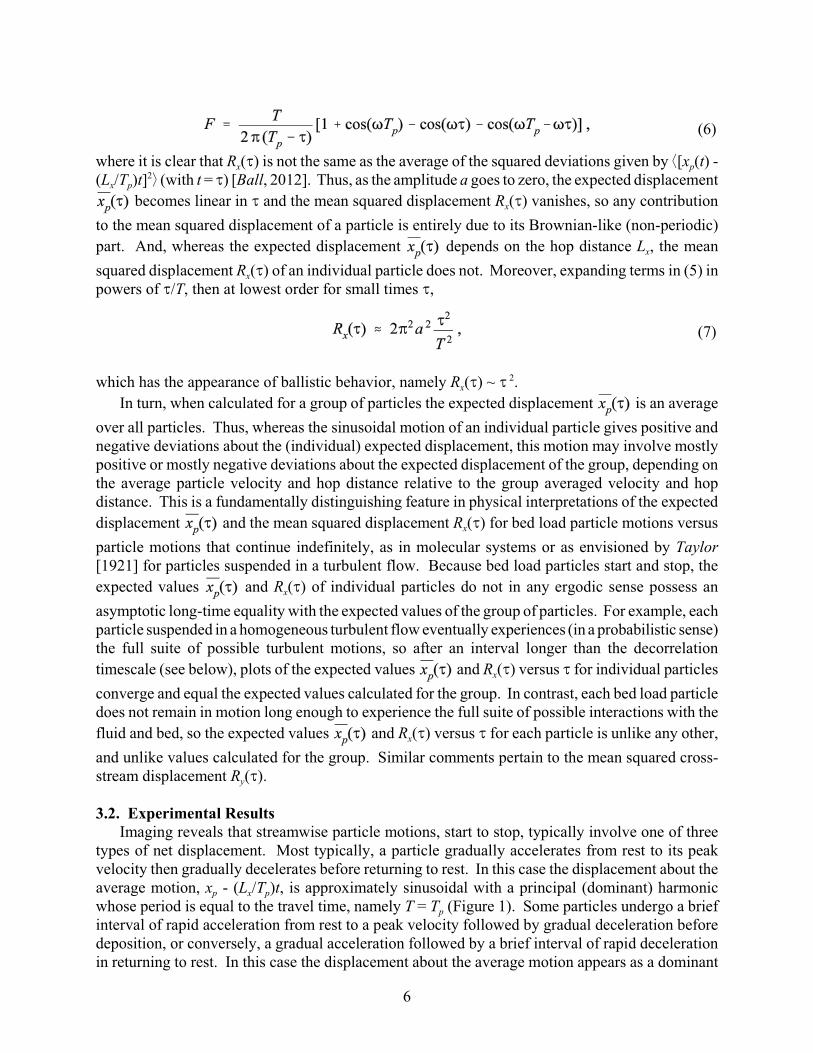
x pThe motion of a particle, start to stop, over a hop distance L during the travel time T by

p p pdefinition starts and ends with zero velocity (u (0) = u (T ) = 0) with finite peak velocity in between.

5

p pSo regardless of how the particle velocity u (t) varies in detail during the interval 0 # t # T , the

p pvelocity signal u (t) must possess at its most basic level a fundamental harmonic with period T = 2T[t] (although variations on this assertion, elaborated below, are possible). Treating this harmonic

pas a sinusoid, it is straightforward to show that integration of the velocity signal u (t) yields a

p x pdisplacement signal x (t) composed of the sum of two parts, a mean motion equal to (L /T )t, and

pa fluctuating motion possessing a fundamental harmonic with period T = T , normally the dominantharmonic [Roseberry et al., 2012; Ball, 2012; but see section 3.2 below] (Figure 1). Moreover, the

ptravel time T of a particle influences the amplitude of its fundamental velocity harmonic and, in

pturn, the amplitude of the harmonic of the fluctuating part of the displacement signal x (t). Namely,particles with long travel times on average are more likely to be accelerated to large peak velocitiesthan are particles with short travel times [Roseberry et al., 2012]. The corollary is that particles with

pshort travel times on average are limited to relatively small peak velocities. For illustration let x (t)

x p p= (L /T )t + asin(2Bt/T ), where a [L] is the amplitude of the dominant (and in this case, the

p pfundamental) harmonic with period T = T . If U [L t ] is the amplitude of the underlying harmonic-1

p p p x pof the velocity signal u (t) with period T = 2T , then U ~ L /T and the amplitude a is directly

p p xproportional to the product U T ~ L .

xConsider the contribution to the mean squared displacement R (J) due to the periodic part of themotion of a particle. We start by assuming that the fundamental, or dominant, harmonic of the

p p x pdisplacement signal x (t) of a particle is given by x (t) = (L /T )t + asin(Tt), where T = 2B/T is the

pangular frequency and the period T is not necessarily equal to the travel time T . The expected

displacement associated with an interval J is

giving

where it becomes clear that is not the same as the average displacement of the particle given

x pby (L /T )t (with t = J). Using the right side of the Einstein-Smoluchowsky equation (1) the mean

xsquared displacement R (J) is

giving

in which the function F is

(2)

(3)

(4)

(5)

6

x pwhere it is clear that R (J) is not the same as the average of the squared deviations given by +[x (t) -

x p(L /T )t] , (with t = J) [Ball, 2012]. Thus, as the amplitude a goes to zero, the expected displacement2

x becomes linear in J and the mean squared displacement R (J) vanishes, so any contribution

to the mean squared displacement of a particle is entirely due to its Brownian-like (non-periodic)

xpart. And, whereas the expected displacement depends on the hop distance L , the mean

xsquared displacement R (J) of an individual particle does not. Moreover, expanding terms in (5) inpowers of J/T, then at lowest order for small times J,

xwhich has the appearance of ballistic behavior, namely R (J) ~ J . 2

In turn, when calculated for a group of particles the expected displacement is an average

over all particles. Thus, whereas the sinusoidal motion of an individual particle gives positive andnegative deviations about the (individual) expected displacement, this motion may involve mostlypositive or mostly negative deviations about the expected displacement of the group, depending onthe average particle velocity and hop distance relative to the group averaged velocity and hopdistance. This is a fundamentally distinguishing feature in physical interpretations of the expected

xdisplacement and the mean squared displacement R (J) for bed load particle motions versus

particle motions that continue indefinitely, as in molecular systems or as envisioned by Taylor[1921] for particles suspended in a turbulent flow. Because bed load particles start and stop, the

xexpected values and R (J) of individual particles do not in any ergodic sense possess an

asymptotic long-time equality with the expected values of the group of particles. For example, eachparticle suspended in a homogeneous turbulent flow eventually experiences (in a probabilistic sense)the full suite of possible turbulent motions, so after an interval longer than the decorrelation

xtimescale (see below), plots of the expected values and R (J) versus J for individual particles

converge and equal the expected values calculated for the group. In contrast, each bed load particledoes not remain in motion long enough to experience the full suite of possible interactions with the

xfluid and bed, so the expected values and R (J) versus J for each particle is unlike any other,

and unlike values calculated for the group. Similar comments pertain to the mean squared cross-

ystream displacement R (J).

3.2. Experimental ResultsImaging reveals that streamwise particle motions, start to stop, typically involve one of three

types of net displacement. Most typically, a particle gradually accelerates from rest to its peakvelocity then gradually decelerates before returning to rest. In this case the displacement about the

p x paverage motion, x - (L /T )t, is approximately sinusoidal with a principal (dominant) harmonic

pwhose period is equal to the travel time, namely T = T (Figure 1). Some particles undergo a briefinterval of rapid acceleration from rest to a peak velocity followed by gradual deceleration beforedeposition, or conversely, a gradual acceleration followed by a brief interval of rapid decelerationin returning to rest. In this case the displacement about the average motion appears as a dominant

(6)

(7)

7

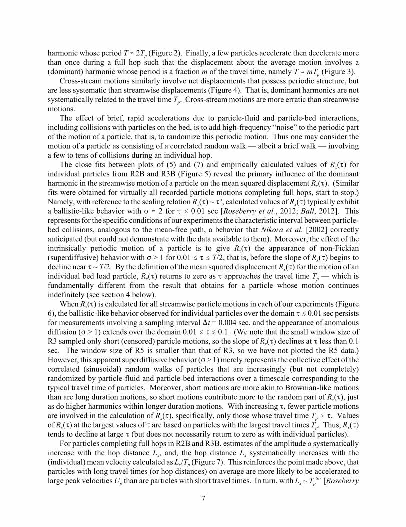
pharmonic whose period T . 2T (Figure 2). Finally, a few particles accelerate then decelerate morethan once during a full hop such that the displacement about the average motion involves a

p(dominant) harmonic whose period is a fraction m of the travel time, namely T . mT (Figure 3).Cross-stream motions similarly involve net displacements that possess periodic structure, but

are less systematic than streamwise displacements (Figure 4). That is, dominant harmonics are not

psystematically related to the travel time T . Cross-stream motions are more erratic than streamwisemotions.

The effect of brief, rapid accelerations due to particle-fluid and particle-bed interactions,including collisions with particles on the bed, is to add high-frequency “noise” to the periodic partof the motion of a particle, that is, to randomize this periodic motion. Thus one may consider themotion of a particle as consisting of a correlated random walk — albeit a brief walk — involvinga few to tens of collisions during an individual hop.

xThe close fits between plots of (5) and (7) and empirically calculated values of R (J) forindividual particles from R2B and R3B (Figure 5) reveal the primary influence of the dominant

xharmonic in the streamwise motion of a particle on the mean squared displacement R (J). (Similarfits were obtained for virtually all recorded particle motions completing full hops, start to stop.)

x xNamely, with reference to the scaling relation R (J) ~ J , calculated values of R (J) typically exhibitF

a ballistic-like behavior with F . 2 for J . 0.01 sec [Roseberry et al., 2012; Ball, 2012]. Thisrepresents for the specific conditions of our experiments the characteristic interval between particle-bed collisions, analogous to the mean-free path, a behavior that Nikora et al. [2002] correctlyanticipated (but could not demonstrate with the data available to them). Moreover, the effect of the

xintrinsically periodic motion of a particle is to give R (J) the appearance of non-Fickian

x(superdiffusive) behavior with F > 1 for 0.01 . J . T/2, that is, before the slope of R (J) begins to

xdecline near J ~ T/2. By the definition of the mean squared displacement R (J) for the motion of an

x pindividual bed load particle, R (J) returns to zero as J approaches the travel time T — which isfundamentally different from the result that obtains for a particle whose motion continuesindefinitely (see section 4 below).

xWhen R (J) is calculated for all streamwise particle motions in each of our experiments (Figure6), the ballistic-like behavior observed for individual particles over the domain J . 0.01 sec persistsfor measurements involving a sampling interval )t = 0.004 sec, and the appearance of anomalousdiffusion (F > 1) extends over the domain 0.01 . J . 0.1. (We note that the small window size of

xR3 sampled only short (censored) particle motions, so the slope of R (J) declines at J less than 0.1sec. The window size of R5 is smaller than that of R3, so we have not plotted the R5 data.)However, this apparent superdiffusive behavior (F > 1) merely represents the collective effect of thecorrelated (sinusoidal) random walks of particles that are increasingly (but not completely)randomized by particle-fluid and particle-bed interactions over a timescale corresponding to thetypical travel time of particles. Moreover, short motions are more akin to Brownian-like motions

xthan are long duration motions, so short motions contribute more to the random part of R (J), justas do higher harmonics within longer duration motions. With increasing J, fewer particle motions

x pare involved in the calculation of R (J), specifically, only those whose travel time T $ J. Values

x p xof R (J) at the largest values of J are based on particles with the largest travel times T . Thus, R (J)tends to decline at large J (but does not necessarily return to zero as with individual particles).

For particles completing full hops in R2B and R3B, estimates of the amplitude a systematically

x xincrease with the hop distance L , and, the hop distance L systematically increases with the

x p(individual) mean velocity calculated as L /T (Figure 7). This reinforces the point made above, thatparticles with long travel times (or hop distances) on average are more likely to be accelerated to

p x plarge peak velocities U than are particles with short travel times. In turn, with L ~ T [Roseberry5/3

8

p x p pet al., 2012], then U ~ L /T ~ T [Ball, 2012]. Thus, whereas the hop distance on average2/3

increases at a growing rate with increasing travel time, the mean velocity increases less rapidly withincreasing travel time.

yWhen R (J) is calculated for all cross-stream motions in each experiment, no ballistic-like

ybehavior is apparent at small J, and the slope F (i.e. the exponent in R (J) ~ J ) over the domain 0.01F

. J . 0.1 varies from about 1 to 1.8 (Figure 8). The magnitudes of cross-stream particle velocitiestypically are much smaller than streamwise velocities [Roseberry et al., 2012], and ourmeasurements of small cross-stream displacements are less precise.

4. Particle Diffusivity4.1. Definition of the Diffusivity

pThe motion of a bed load particle over its travel time T is continuous, albeit involving quasi-random (high-frequency) fluctuations in the velocity associated with fluid accelerations and particle-bed collisions [Lajeunesse et al., 2010; Roseberry et al., 2012; Furbish et al., 2012b]. An

x yappropriate description of the particle diffusivities 6 and 6 therefore can be obtained from theclassic definition provided by Taylor [1921]. It is important, however, to be explicit about theaveraging involved in this definition, inasmuch as G. I. Taylor envisioned particle motions thatcontinue indefinitely, as opposed to the start-and-stop motions of bed load particles.

As described in Furbish et al. [2012a] and Roseberry et al. [2012], consider a planar streambedarea B [L ] large enough to fully sample steady, homogeneous near-bed conditions of turbulence and2

transport. At any instant the number N of active particles is approximately constant. That is, therate of disentrainment within B equals the rate of entrainment, and the rate at which particles leaveB across its boundaries equals the rate at which particles enter B across its boundaries. Imagine

srecording particle motions within B for an interval of time T [t] [e.g. Lajeunesse et al., 2010;

sRoseberry et al., 2012]. For T much longer than the mean particle travel time (also see below),

sparticle motions during T adequately represent the joint probability density [L-2

x y pt ] of hop distances L and L , and travel times T [Furbish et al., 2012a] without bias due to-1

scensorship of motions at times t = 0 and t = T [Furbish et al., 1990]. The marginal probability

densities [L ], [L ] and [t ] possess the means [L], [L] and [t].-1 -1 -1

Moreover, at any instant the velocities of active particles within B possess the probability densities

[L t] and [L t] with means [L t ] and [L t ] and variances [L t ] and [L-1 -1 -1 -1 2 -2 2

t ], where it may be assumed that these represent ensemble averaged quantities [Furbish et al.,-2

2012a, 2012b; Roseberry et al., 2012].

p iThe average streamwise velocity of the ith active particle with travel time T is

s s sIn turn, letting N denote the number of particle motions during T (note that N o N), and assuming

sthat N is large, the ensemble average velocity

(8)

9

Thus, contrary to the assertion of Lajeunesse et al. [2010], the ensemble average hop distance

is equal to the product of the ensemble averaged velocity and the mean travel time . (But note

x i p ithat � +L /T ,.)

As a point of reference, when particles continue their motions indefinitely (that is, they do not

p i sstart and stop), then experimentally T = T (the sample time) and (9) becomes

swhere now is the average displacement during T , and the average in (10) is the same as the

average of an individual particle over long time.

p i p i xLetting u N = u - , then the autocovariance C (J) [L t ] of the streamwise particle velocities2 -2

is

where

p J s xis the number of particle motions with travel time T $ J. When J = 0, N = N , and C (0) = .

And, when particles continue their motions indefinitely,

Taylor [1921] demonstrated that for continuous particle motions,

Inasmuch as the integral in (14) converges as J 6 4, then the streamwise particle diffusivity is

(9)

(10)

(11)

(12)

(13)

(14)

(15)

10

Lin which J [t] is the Lagrangian integral timescale defined by

x xwhere A (J) = C (J)/ is the autocorrelation of the streamwise particle velocities. Note that in this

s Ldevelopment we are envisioning T o J . By a similar development the cross-stream diffusivity is

pwhere is the variance of the cross-stream velocities v .

4.2. Experimental Results

xThe autocovariance C (J) decays to zero by about J . 0.1 sec for our experiments (Figure 9).In turn, the integral in (15) converges, where numerically computed values level off at J . 0.1 to

x0.15 sec (Figure 10), giving estimates of 6 from about 0.3 cm s to 0.8 cm s over the range of2 -1 2 -1

experimental conditions. Inasmuch as variations in particle velocity are of the same order as the

mean velocity , [Roseberry et al., 2012; Furbish et al., 2012b], then as suggested by Phillips

[1991],

L xwhere * ~ J [L] is a characteristic distance of motion over which the autocovariance C (J) is

significant, and is similar in magnitude to the mean hop distance. Moreover, there is clear evidence

pthat particles velocities u possess an exponential density with ensemble average

[Lajeunesse et al., 2010; Roseberry et al., 2012; Furbish et al., 2012b], in which case ,

xwhich reinforces the point in (18), that 6 ~ *. In the language of transport in porous media flows,

* is the so-called “dispersivity.” In addition, estimates of the Lagrangian integral timescale suggest

Lthat J . 0.1 sec, similar to the mean travel time estimated for particles in R2B and R3B [Roseberry

et al., 2012]. We may therefore assume that , where k is a dimensionless

factor of order unity.

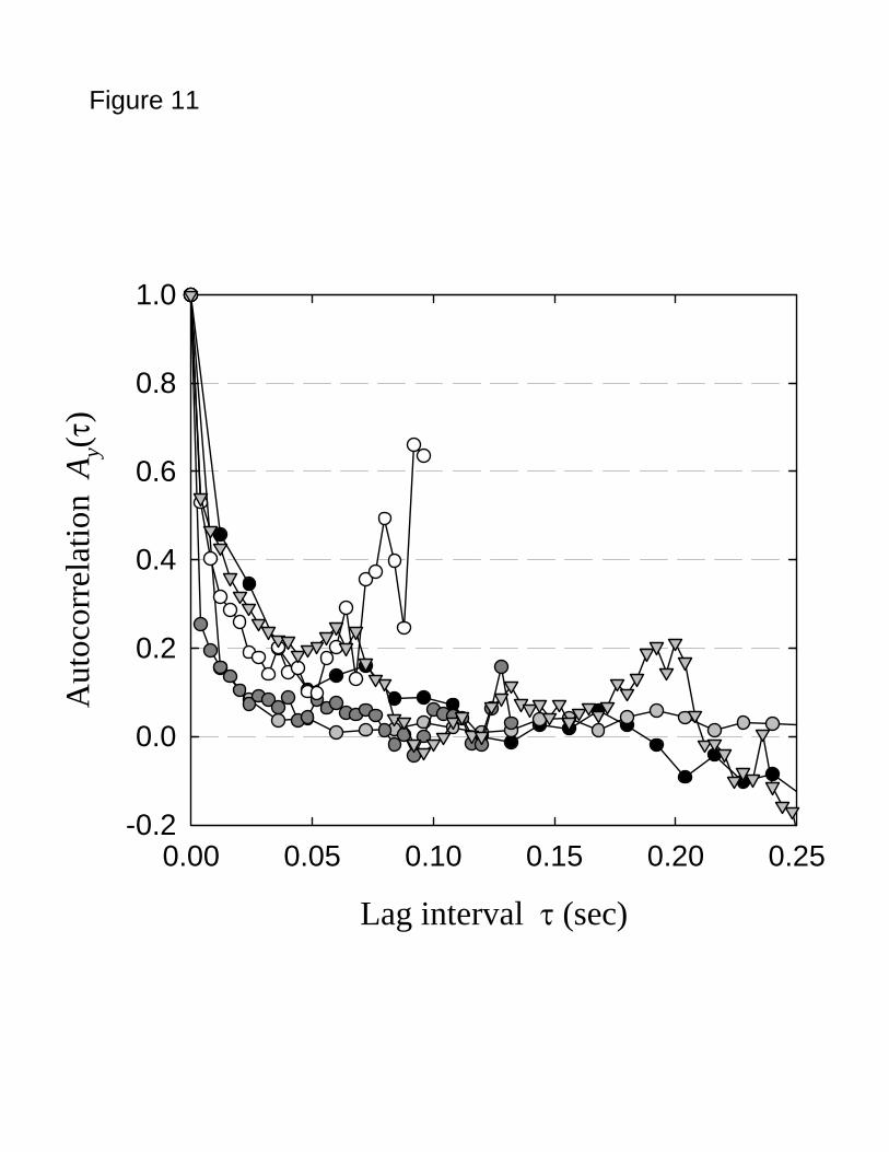
yFor cross-stream motions the autocovariance C (J) decays to zero by about J . 0.1 sec (Figure11). The integral in (17) converges, where numerically computed values level off at J . 0.1 sec

y(Figure 12), giving estimates of 6 from about 0.05 cm s to 0.1 cm s over the range of2 -1 2 -1

xexperimental conditions, approximately an order of magnitude smaller than values of 6 .

x yWe emphasize that calculated values of C (J) and C (J) at a given interval J are based on all

pvelocity signals for which T $ J. Thus, for small J these values are based on the velocity signalsof most particles in each experiment, and for large J these values are based on fewer signals with

x y x ylonger travel times. Uncertainty in the estimates of C (J) and C (J) (or A (J) and A (J)) therefore

Lincreases with increasing J. Estimates at J o J cannot be interpreted as being significantly differentfrom zero.

(16)

(17)

(18)

11

5. Discussion and ConclusionsAs pointed out in Roseberry et al. [2012], problems of diffusion in molecular systems typically

involve processes in which an individual particle experiences, say, 10 - 10 collisions per second.6 10

Motions continue indefinitely, and any scale invariant superdiffusive behavior (as characterized, forexample, by hard sphere theory) emerges rapidly and persists. In ecological systems, hundreds tothousands of “collisions” (meaning changes in direction) of a “particle” — such as an albatross ora honey bee — can occur during an individual Lévy flight [Viswanathan et al., 1996; Reynolds etal., 2007]. In contrast, the sediment particle motions described herein involve a few to tens ofcollisions with the bed during one particle hop. The (apparent) superdiffusive behavior manifest in

xplots of the mean squared displacement R (J) over a timescale 0.01. J . 0.1 sec actually reflects theeffects of periodicities that are inherent in streamwise particle motions, not (scale invariant)superdiffusion — a behavior that cannot in any case persist at longer timescales.

The idea that bed load particle motions exhibit a ballistic-like behavior at small time intervalsJ is not the same as ballistic behavior as (conventionally) defined for molecular systems in whichparticles travel unimpeded within a vacuum between collisions. For example, because the mean-freetime and associated mean-free path of air molecules are small at Earth-surface pressure andtemperature conditions, molecular motions can be approximated as straight lines with constantvelocity between collisions. (In detail these motions are parabolic in Earth’s gravitational field,decidedly so at the rarified conditions of the outer atmosphere.) In contrast, bed load particlemotions are strongly coupled with fluid motions, and particles rarely move faster than the fluid.Insofar as bed load particles travel at approximately constant velocity between collisions with the

xbed — leading to R (J) ~ J — then this is a result of the particle-fluid coupling, not true ballistic2

behavior. The magnitudes of cross-stream particle velocities typically are much smaller thanstreamwise velocities [Roseberry et al., 2012], and the absence of ballistic-like behavior in plots of

yR (J) at small J likely reflects imprecision in our measurements of small (cross-stream) particledisplacements.

At any instant, and from one instant to the next, the N active particles within the streambed areaB represent all possible stages of motions over each possible particle hop represented by theunderlying distribution of hop distances, and . It is therefore appropriate to calculate

x y x y p p p pR (J), R (J), C (J) and C (J) based on all paired observations of x , y , u and v separated by theinterval J (as opposed to setting the initial time t of each motion to zero and calculating averagesonly across the number of motions for each time J) in order to ensure that these quantities represent

x xensemble averages. For example, a value of R (J) or C (J) calculated for small J includes thoseparticles near the end of long hops as well as those near the beginning of short hops and long hops,in proportion to the likely occurrence of the various stages of motion of the N active particlessampled from all hops at any instant.

x yThat the autocovariances C (J) and C (J) decay to zero over a short interval J indicates aFickian-like diffusive behavior [Taylor, 1921; Garrett, 2006; Ferrari, 2007] in both streamwise and

xcross-stream particle motions. In contrast, if C (J), for example, possesses a long tail, then (15) does

Lnot converge rapidly and the diffusivity increases, albeit slowly, at times larger than J [Garrett,2006]. But here it is important to reemphasize that bed load particle motions do not continue

x Lindefinitely, so in fact a finite C (J) for J o J is not physically meaningful in characterizingdiffusive behavior. More basically, a Fickian-like behavior is anticipated from the exponential-like

p pparticle velocity distributions of u and v , possibly involving “light” tails [Roseberry et al., 2012;Furbish et al., 2012b], where the diffusivity arises from the time derivative of the second momentof the underlying probability density function of particle displacements occurring during a small

12

x yinterval dt [Furbish et al., 2012a]. The rapid decay of C (J) and C (J) over J provides a clearer

x ymeasure of diffusive behavior than does the form of R (J) or R (J), which is intrinsically sensitive

Lto effects of periodicities in particle motions that start and stop with an average travel time ~ J .

As described in companion papers [Furbish et al., 2012a, 2012b], the volumetric bed loadsediment flux involves an advective part equal to the product of the average particle velocity andthe particle activity (the solid volume of particles in motion per unit streambed area), and a diffusivepart involving the gradient of the product of the particle activity and the diffusivity. This diffusivecontribution to the flux may be important under conditions of nonuniform transport, and Taylor’sformulation of the diffusivity, as described above, yields a proper description of the diffusion of bedload particles at low transport rates, consistent with Fickian diffusion. The problem of diffusion(dispersion) of tracer particles involving the effects of multiple hops and rest times [Sayre andHubbell, 1965; Drake et al., 1988; Hassan and Church, 1991; Ferguson and Wathen, 1998; Nikoraet al., 2002; Martin et al., 2012] requires a different formalism [Bradley et al., 2010; Ganti et al.,2010; Hill et al., 2010].

The analysis also points to the design of experimental measurements required to obtain preciseestimates of the particle diffusivity and related quantities. Here are lessons we have learned. Toconfidently estimate the displacement and velocity statistics described above, including the meanhop distance and travel time (and their distributions), the sampling window size and time interval

sare critical. The window must be large enough, and the sampling time must be long enough (T o

LJ ), to obtain a sufficient count of hops representing the full range of hop distances occurring in thenear-bed conditions of turbulence. Our runs R2B and R3B, like R1 and R2, had sufficiently largewindows, but suffered from short sampling times. Runs R3 and R5, like R1 and R2, involvedsufficient sampling times, but suffered from small windows. Moreover, to see ballistic-like behaviorrequires a sampling interval shorter than the typical interval between particle-bed collisions.Experiments involving a wider range of flow conditions and particle sizes are required to clarify therelation between particle velocities and diffusivities as suggested in section 4.2.

Notationa amplitude of sinusoidal particle displacement [L].

x yA , A autocorrelation of streamwise and cross-stream particle velocities.B streambed area [L ].2

x yC , C autocovariance of streamwise and cross-stream particle velocities [L t ].2 -2

D particle diameter [L].probability density functions of streamwise and cross-stream particle hop distances

[L ].-1

probability density function of particle travel times [t ].-1

joint probability density function of particle hop distances and travel times [L t ].-1 -1

probability density functions of streamwise and cross-stream particle velocities [L-1

t].F function defined by (6).k dimensionless factor of order unity.

x yL , L streamwise and cross-stream particle hop distances [L].m fraction of travel time.N number of active particles within the streambed area B.

13

s sN number of particle motions during the sampling interval T .

J pN number of particle motions with travel time T $ J.

x yR , R mean squared streamwise and cross-stream particle displacements [L ].2

t time [t].T period of sinusoidal particle displacement [t].

pT particle travel time [t].

sT sampling interval [t].

pu streamwise particle velocity [L t ].-1

pu N deviation in streamwise particle velocity about the average [L t ].-1

pU amplitude of sinusoidal particle velocity [L t ].-1

pv cross-stream particle velocity [L t ].-1

px streamwise particle position or displacement [L].

px particle position or displacement vector [L].

py cross-stream particle position or displacement [L].

0z roughness length [L].

L* characteristic distance of particle motion during J [L].

x y6 , 6 streamwise and cross-stream particle diffusivities [L t ].2 -1

F exponent in scaling relation R(J) ~ J .F

variance of streamwise and cross-stream particle velocities [L t ].2 -2

J time (lag) interval [t].

LJ Lagrangian integral timescale [t].T angular frequency equal to 2B/T [t ].-1

Acknowledgments. We are grateful to Peter Haff for critical discussions and insight. We acknowledge support by theNational Science Foundation (EAR-0744934). All data described herein are available to the community.

ReferencesBall, A. E. (2012), Measurements of bed load particle diffusion at low transport rates, Junior thesis, Vanderbilt University,

Nashville, Tennessee.Bradley, D. N., G. E. Tucker, and D. A. Benson (2010), Fractional dispersion in a sand bed river, Journal of Geophysical

Research – Earth Surface, 115, F00A09, doi: 10.1029/2009JF001268.Cantrell, R. S., and C. Cosner (2003), Spatial Ecology via Reaction-Diffusion Equations, John Wiley & Sons, Chichester.Drake, T. G., R. L. Shreve, W. E. Dietrich, P. J. Whiting, and L. B. Leopold (1988), Bedload transport of fine gravel observed

by motion-picture photography, Journal of Fluid Mechanics, 192, 193-217.Einstein, A. (1905), Über die von der molekularkinetischen Theorie der Wärme geforderte Bewegung von in ruhenden

Flüssigkeiten suspendierten Teilchen, Annalen der Physik, 17, 549-560.Einstein, H. A. (1937), Bedload transport as a probability problem, Ph.D. thesis, Mitt. Versuchsanst. Wasserbau Eidg. Tech.

Hochsch, Zürich.Einstein, H. A. (1950), The bed-load function for sediment transportation in open channel flows, Technical Bulletin 1026,

Soil Conservation Service, U.S. Department of Agriculture, Washington, D.C.Ferguson, R. I., and S. J. Wathen (1998), Tracer-pebble movement along a concave river profile: Virtual velocity in relation

to grain size and shear stress, Water Resources Research, 34, 2031-2038.Ferrari, R. (2007), Statistics of dispersion in flows with coherent structures, Proceedings, The 15 ‘Aha Huliko’a Winterth

Workshop, 23-26 January, Honolulu, sponsored by the U.S. Office of Naval Research and the University of Hawaii.Furbish, D. J., E. M. Childs, P. K. Haff, and M. W. Schmeeckle (2009a), Rain splash of soil grains as a stochastic advection-

dispersion process, with implications for desert plant-soil interactions and land-surface evolution, Journal of GeophysicalResearch – Earth Surface, 114, F00A03, doi: 10.1029/2009JF001265.

Furbish, D. J., and P. K. Haff (2010), From divots to swales: Hillslope sediment transport across divers length scales, Journalof Geophysical Research – Earth Surface, 115, F03001, doi: 10.1029/2009JF001576.

Furbish, D. J., P. K. Haff, W. E. Dietrich, and A. M. Heimsath (2009b), Statistical description of slope-dependent soiltransport and the diffusion-like coefficient, Journal of Geophysical Research – Earth Surface, 114, F00A05, doi:

14

10.1029/2009JF001267.Furbish, D. J., P. K. Haff, J. C. Roseberry, and M. W. Schmeeckle (2012a), A probabilistic description of the bed load

sediment flux: 1. Theory. (submitted as a companion paper)Furbish, D. J., J. C. Roseberry, and M. W. Schmeeckle (2012b), A probabilistic description of the bed load sediment flux:

3. The particle velocity distribution and the diffusive flux. (submitted as a companion paper)Ganti, V., M. M. Meerschaert, E. Foufoula-Georgiou, E. Viparelli, and G. Parker (2010), Normal and anomalous diffusion

of gravel tracer particles in rivers, Journal of Geophysical Research – Earth Surface, 115, F00A12, doi:10.1029/2008JF001222.

Garrett, C. (2006), Turbulent dispersion in the ocean, Progress in Oceanography, 70, 113-125, doi:10.1016/j.pocean.2005.07.005.

Hassan, M. A., and M. Church (1991), Distance of movement of coarse particles in gravel bed streams, Water ResourcesResearch, 27, 503-511.

Hill, K. M., L. DellAngelo, and M. M. Meerschaert (2010), Heavy-tailed travel distance in gravel bed transport: Anexploratory enquiry, Journal of Geophysical Research – Earth Surface, 115, F00A14, doi: 10.1029/2009JF001276.

Lajeunesse, E., L. Malverti, and F. Charru (2010), Bed load transport in turbulent flow at the grain scale: Experiments andmodeling, Journal of Geophysical Research – Earth Surface, 115, F04001, doi: 10.1029/2009JF001628.

Lisle, I. G., C. W. Rose, W. L. Hogarth, P. B. Hairsine, G. C. Sander, and J. Y. Parkange (1998), Stochastic sedimenttransport in soil erosion, Journal of Hydrology, 204, 217-230.

Martin, R. L., D. J. Jerolmack, and R. Schumer (2012), The physical basis for anomalous diffusion in bedload transport,Journal of Geophysical Research – Earth Surface, doi: 10.1029/2011JF002075. (in press)

Metzler, R., and J. Klafter (2000), The random walk’s guide to anomalous diffusion: a fractional dynamics approach, PhysicsReports, 339, 1-77.

Nikora, V., H. Habersack, T. Huber, and I. McEwan (2002), On bed particle diffusion in gravel bed flows under weak bedload transport, Water Resources Research, 38, 1081, doi: 10.1029/2001WR000513.

Okubo, A., and S. A. Levin (Eds.) (2001), Diffusion and Ecological Problems: Modern Perspectives (Second Edition),Springer-Verlag, New York.

Phillips. O. M. (1991), Flow and reactions in permeable rocks, Cambridge University Press, Cambridge.Reynolds, A. M., A. D. Smith, R. Menzel, U, Greggers, D. R. Reynolds, and J. R. Riley (2007), Displaced honey bees

perform optimal scale-free search flights, Ecology, 88, 1955-1961.Roseberry, J. C., M. W. Schmeeckle, and D. J. Furbish (2012), A probabilistic description of the bed load sediment flux: 2:

Particle activity and motions. (submitted as a companion paper)Sayre, W., and D. Hubbell (1965), Transport and dispersion of labeled bed material, North Loup River, Nebraska, U.S.

Geological Survey Professional Paper, 433-C, 48 pp.Schmeeckle, M. W., and D. J. Furbish (2007), A Fokker-Planck model of bedload transport and morphodynamics, Abstract

presented at the Stochastic Transport and Emerging Scaling on Earth’s Surface (STRESS) work group meeting, LakeTahoe, Nevada, sponsored by National Center for Earth-surface Dynamics, the University of Illinois, and the DesertResearch Institute.

Schumer, R., M. M. Meerschaert, and B. Baeumer (2009), Fractional advection-dispersion equations for modeling transportat the Earth surface, Journal of Geophysical Research – Earth Surface, 114, F00A07, doi: 10.1029/2008JF001246.

Taylor, G. I. (1921), Diffusion by continuous movements, Proceedings of the London Mathematical Society, 20, 196-211.Trigger, S. A. (2010), Anomalous transport in velocity space: from Fokker-Planck to the general equation, Journal of Physics

A: Mathematical and Theoretical, 43, doi: 10.1088/1751-8113/43/28/285005.Viswanathan, G, M., V. Afanasyev, S. V. Buldyrev, E. J. Murphy, P. A. Prince, and H. E. Stanley (1996), Lévy flight search

patterns of wandering albatrosses, Nature, 381, 413-415.Viswanathan, G. M., E. P. Raposo, F. Bartumeus, J. Catalan, and M. G. E. Da Luz (2005), Necessary criterion for

distinguishing true superdiffusion from correlated random walk processes, Physical Review E, 72, 011111, doi:10.1103/PhysRevE.72.011111.

______________A. E. Ball, Department of Earth and Environmental Sciences, Vanderbilt University, 2301 Vanderbilt Place, Station B

35-1805, Nashville, Tennessee 37235, USA. (ashley.e.ball@vanderbilt.edu)D. J. Furbish, Department of Earth and Environmental Sciences, Vanderbilt University, 2301 Vanderbilt Place, Station

B 35-1805, Nashville, Tennessee 37235, USA. (david.j.furbish@vanderbilt.edu)M. W. Schmeeckle, School of Geographical Sciences, Arizona State University, Tempe, Arizona 85287, USA.

(schmeeckle@asu.edu)

15

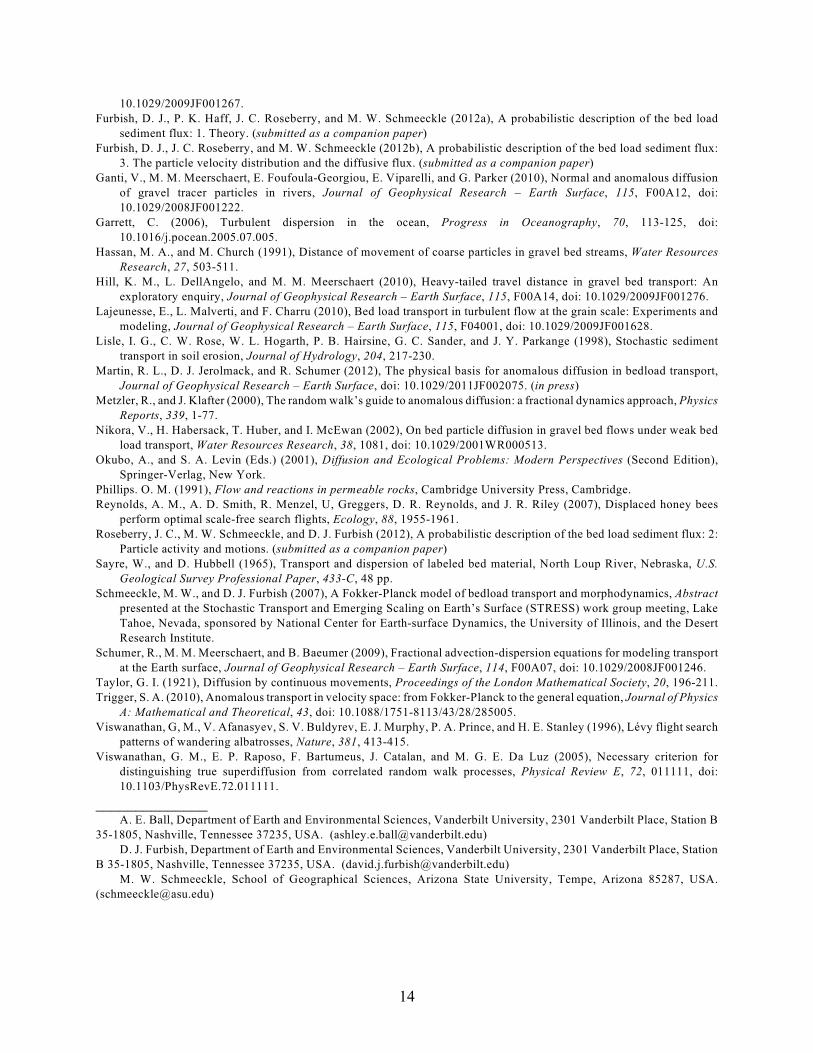
Figure CaptionspFigure 1. Plot of examples of (a) streamwise particle displacement x versus time t and (b)

p pdeviation in particle displacement about the average motion, x - (L/T )t, versus time t forparticles that gradually accelerate from rest to their peak velocities then gradually deceleratebefore returning to rest; in this case the displacement about the average motion is approximatelysinusoidal with a principal (dominant) harmonic whose period T is equal to the travel time,

pnamely T = T .

pFigure 2. Plot of examples of (a) streamwise particle displacement x versus time t and (b)

p pdeviation in particle displacement about the average motion, x - (L/T )t, versus time t forparticles that undergo a brief interval of rapid acceleration from rest to a peak velocity followedby gradual deceleration before deposition, or conversely, a gradual acceleration followed by abrief interval of rapid deceleration in returning to rest; in this case the displacement about the

paverage motion appears as a dominant harmonic whose period T . 2T .

pFigure 3. Plot of examples of (a) streamwise particle displacement x versus time t and (b)

p pdeviation in particle displacement about the average motion, x - (L/T )t, versus time t forparticles that accelerate then decelerate more than once during a full hop such that thedisplacement about the average motion involves a (dominant) harmonic whose period T is a

pfraction m of the travel time, namely T . mT .

pFigure 4. Plot of cross-stream particle displacements y versus time t for particles motionsillustrated in (a) Figure 1 and (b) Figure 2.

Figure 5. Plots of calculated (circles) and theoretical (solid lines) values of the mean squared

xdisplacement R (J) versus time interval J for particle motions illustrated in (a) Figure 1 with T

p p p p= T , (b) Figure 2 with T = 2T , and (c) Figure 3 with T = 0.5T (black), T = 0.4T (light gray),

p pT = 0.7T (dark gray) and T = 0.5T (white); dashed lines are given by (7) and possess slopes ofF = 2.

xFigure 6. Plot of mean squared displacement R (J) versus time interval J for all particle motionswithin experiment R1 (black), R2 (light gray circles), R3 (white circles), R2B (light gray

xtriangles) and R3B (white triangles; eye-fit estimates of the slope of R (J) over the domain 0.01. J . 0.1 sec vary from about 1.5 to 1.8, and dashed line possesses slope of F = 2.

Figure 7. Plot of (a) amplitude a versus hop distance L and (b) hop distance L versus mean velocity

pL/T for particles completing full hops in R2B (white) and R3B (black); not shown is one datumin (a) with coordinates (L, a) = (2.31, 0.74).

yFigure 8. Plot of mean squared displacement R (J) versus time interval J for all particle motions

ywithin each experiment; eye-fit estimates of the slope of R (J) over the domain 0.01 . J . 0.1sec vary from about 1 to 1.8.

x x pFigure 9. Plot of autocorrelation A (J) = C (J)/ of streamwise particle velocities u calculated

for R1 (black), R2 (light gray circles), R3 (dark gray circles), R5 (white), R2B (light graytriangles) and R3B (dark gray triangles).

x pFigure 10. Plot of integral of the autocovariance C (J) of streamwise particle velocities ucalculated for R1 (black), R2 (light gray circles), R3 (dark gray circles), R5 (white), R2B (lightgray triangles) and R3B (dark gray triangles).

y y pFigure 11. Plot of autocorrelation A (J) = C (J)/ of cross-stream particle velocities v calculated

for R1 (black), R2 (light gray circles), R3 (dark gray circles), R5 (white) and R2B (light graytriangles).

y pFigure 12. Plot of integral of the autocovariance C (J) of cross-stream particle velocities v

16

calculated for R1 (black), R2 (light gray circles), R3 (dark gray circles), R5 (white) and R2B(light gray triangles).

Table 1. Experimental Conditions.

Run Sampling window

size (pixels)

Run time

(sec)

Sampling

interval (sec)

Mean activity

(number cm )-2

Mean particle velocity

(cm s )-1

R1 500 × 500 18.3 0.012 0.0447 3.45

R2 300 × 300 19.6 0.012 1.00 4.33

R3 100 × 100 13.2 0.004 4.12 5.02

R5 50 × 50 3.5 0.004 21.3 5.46

R2B 1280 × 1024 0.4 0.004 0.190 3.43

R3B 1280 × 1024 0.4 0.004 2.83 4.57

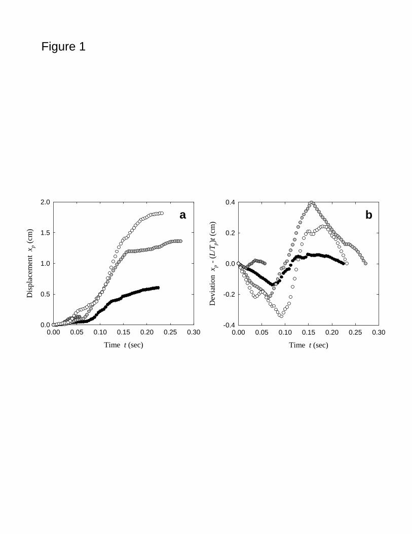
Figure 1

Time t (sec)

0.00 0.05 0.10 0.15 0.20 0.25 0.30

Dis

plac

emen

t x p

(cm

)

0.0

0.5

1.0

1.5

2.0

Time t (sec)

0.00 0.05 0.10 0.15 0.20 0.25 0.30

Dev

iati

on x

p -

(L/T

p)t (

cm)

-0.4

-0.2

0.0

0.2

0.4

a b

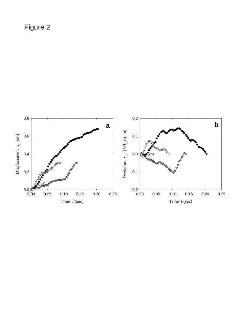
Figure 2

Time t (sec)

0.00 0.05 0.10 0.15 0.20 0.25

Dis

plac

emen

t x p

(cm

)

0.0

0.2

0.4

0.6

0.8

Time t (sec)

0.00 0.05 0.10 0.15 0.20 0.25

Dev

iati

on x

p -

(L/T

p)t (

cm)

-0.2

-0.1

0.0

0.1

0.2

a b

Figure 3

Time t (sec)

0.0 0.1 0.2 0.3 0.4

Dis

plac

emen

t x p

(cm

)

0.0

0.5

1.0

1.5

2.0

2.5

3.0

Time t (sec)

0.0 0.1 0.2 0.3 0.4

Dev

iati

on x

p -

(L/T

p)t (

cm)

-0.2

-0.1

0.0

0.1

0.2

0.3

0.4

a b

Figure 4

Time t (sec)

0.00 0.05 0.10 0.15 0.20 0.25 0.30

Dis

plac

emen

t y p

(cm

)

-0.1

0.0

0.1

0.2

0.3

0.4

0.5

Time t (sec)

0.00 0.05 0.10 0.15 0.20 0.25

Dis

plac

emen

t y p

(cm

)

-0.20

-0.15

-0.10

-0.05

0.00

0.05

0.10

a b

Figure 5

0.001 0.01 0.1 1

Rx()

(cm

2 )

0.00001

0.0001

0.001

0.01

0.1

0.001 0.01 0.1 1

Rx()

(cm

2 )

0.00001

0.0001

0.001

0.01

Time interval (sec)

0.001 0.01 0.1 1

Rx()

(cm

2 )

0.00001

0.0001

0.001

0.01

0.1

a

b

c

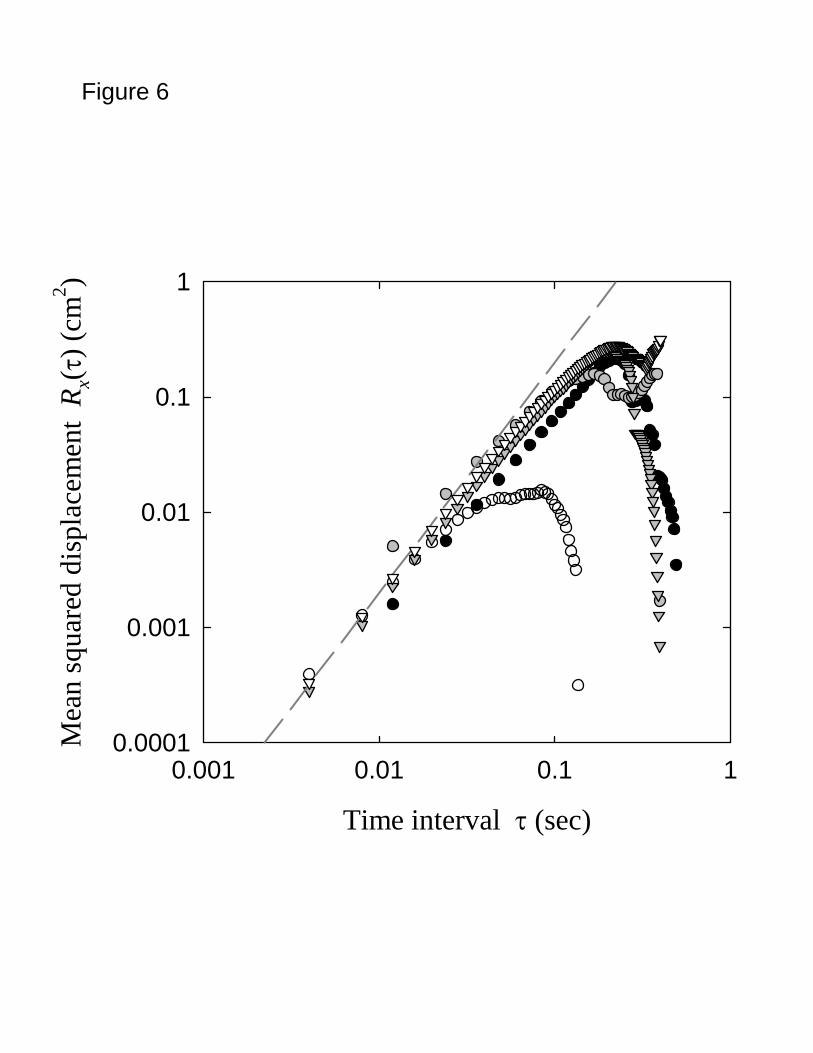
Figure 6

Time interval (sec)

0.001 0.01 0.1 1

Mea

n sq

uare

d di

spla

cem

ent

Rx()

(cm

2 )

0.0001

0.001

0.01

0.1

1

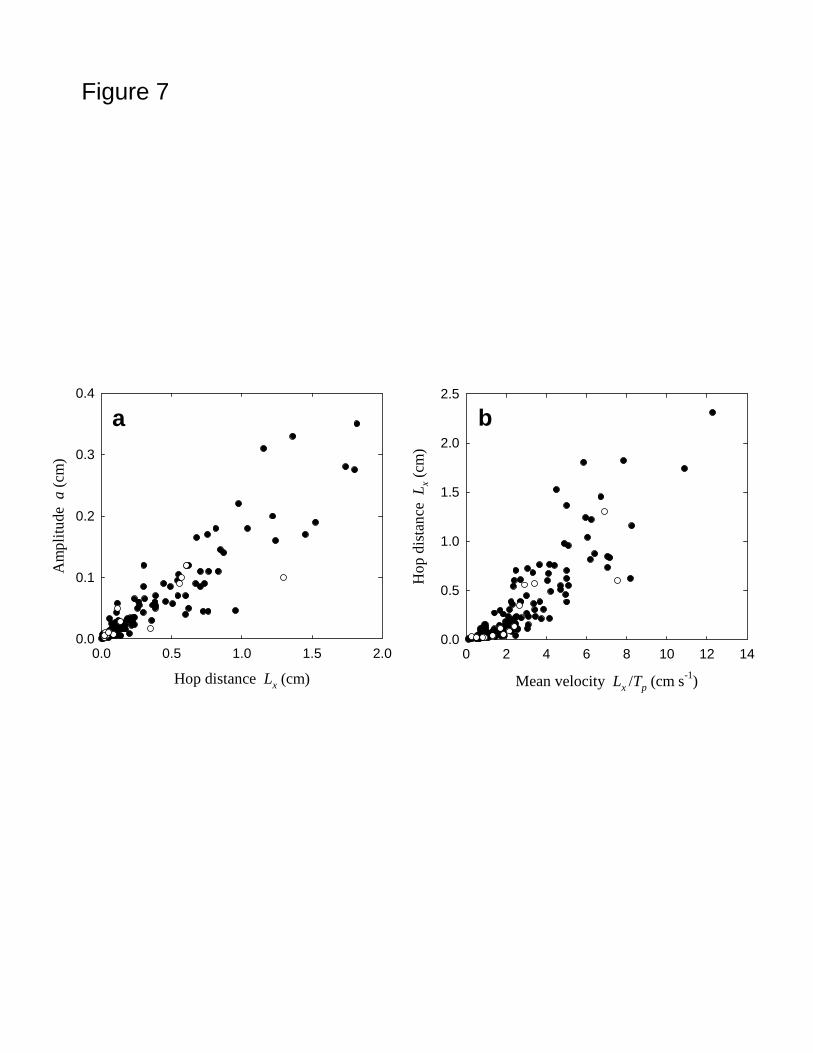
Figure 7

Hop distance Lx (cm)

0.0 0.5 1.0 1.5 2.0

Am

plit

ude

a (

cm)

0.0

0.1

0.2

0.3

0.4

Mean velocity Lx /Tp (cm s-1)

0 2 4 6 8 10 12 14

Hop

dis

tanc

e L

x (cm

)

0.0

0.5

1.0

1.5

2.0

2.5

a b

Time interval (sec)

0.001 0.01 0.1 1

Ry()

(cm

2 )

0.00001

0.0001

0.001

0.01

0.1

1

Figure 8

Lag interval (sec)

0.00 0.05 0.10 0.15 0.20 0.25

Aut

ocor

rela

tion

Ax()

-0.5

0.0

0.5

1.0

Figure 9

Lag interval (sec)

0.00 0.05 0.10 0.15 0.20 0.25

Inte

gral

of

cova

rian

ce C

x()

(cm

2 s-1

)

0.0

0.2

0.4

0.6

0.8

1.0

Figure 10

Lag interval (sec)

0.00 0.05 0.10 0.15 0.20 0.25

Aut

ocor

rela

tion

Ay()

-0.2

0.0

0.2

0.4

0.6

0.8

1.0

Figure 11

Lag interval (sec)

0.00 0.05 0.10 0.15 0.20 0.25

Inte

gral

of

cova

rian

ce C

y()

(cm

2 s-1

)

0.00

0.05

0.10

0.15

0.20

Figure 12