A Predictive Model Which Uses Descriptors of RNA Secondary ...
70
East Tennessee State University Digital Commons @ East Tennessee State University Electronic eses and Dissertations Student Works 5-2011 A Predictive Model Which Uses Descriptors of RNA Secondary Structures Derived from Graph eory. Alissa Ann Rockney East Tennessee State University Follow this and additional works at: hps://dc.etsu.edu/etd Part of the Biochemistry, Biophysics, and Structural Biology Commons , and the Discrete Mathematics and Combinatorics Commons is esis - Open Access is brought to you for free and open access by the Student Works at Digital Commons @ East Tennessee State University. It has been accepted for inclusion in Electronic eses and Dissertations by an authorized administrator of Digital Commons @ East Tennessee State University. For more information, please contact [email protected]. Recommended Citation Rockney, Alissa Ann, "A Predictive Model Which Uses Descriptors of RNA Secondary Structures Derived from Graph eory." (2011). Electronic eses and Dissertations. Paper 1300. hps://dc.etsu.edu/etd/1300
Transcript of A Predictive Model Which Uses Descriptors of RNA Secondary ...

East Tennessee State UniversityDigital Commons @ East
Tennessee State University
Electronic Theses and Dissertations Student Works
5-2011
A Predictive Model Which Uses Descriptors ofRNA Secondary Structures Derived from GraphTheory.Alissa Ann RockneyEast Tennessee State University
Follow this and additional works at: https://dc.etsu.edu/etd
Part of the Biochemistry, Biophysics, and Structural Biology Commons, and the DiscreteMathematics and Combinatorics Commons
This Thesis - Open Access is brought to you for free and open access by the Student Works at Digital Commons @ East Tennessee State University. Ithas been accepted for inclusion in Electronic Theses and Dissertations by an authorized administrator of Digital Commons @ East Tennessee StateUniversity. For more information, please contact [email protected].
Recommended CitationRockney, Alissa Ann, "A Predictive Model Which Uses Descriptors of RNA Secondary Structures Derived from Graph Theory."(2011). Electronic Theses and Dissertations. Paper 1300. https://dc.etsu.edu/etd/1300

A Predictive Model Which Uses Descriptors of
RNA Secondary Structures Derived from Graph Theory
A thesis
presented to
the faculty of the Department of Mathematics and Statistics
East Tennessee State University
In partial fulfillment
of the requirements for the degree
Master of Science in Mathematical Sciences
by
Alissa A. Rockney
May 2011
Debra Knisley Ph.D., Chair
Jeff Knisley, Ph.D.
Teresa Haynes, Ph.D.
Keywords: Graph Theory, RNA, Neural Network, Graphical Invariants

ABSTRACT
A Predictive Model Which Uses Descriptors of
RNA Secondary Structures Derived from Graph Theory
by
Alissa A. Rockney
The secondary structures of ribonucleic acid (RNA) have been successfully modeled
with graph-theoretic structures. Often, simple graphs are used to represent secondary
RNA structures; however, in this research, a multigraph representation of RNA is
used, in which vertices represent stems and edges represent the internal motifs. Any
type of RNA secondary structure may be represented by a graph in this manner. We
define novel graphical invariants to quantify the multigraphs and obtain character-
istic descriptors of the secondary structures. These descriptors are used to train an
artificial neural network (ANN) to recognize the characteristics of secondary RNA
structure. Using the ANN, we classify the multigraphs as either RNA-like or not
RNA-like. This classification method produced results similar to other classification
methods. Given the expanding library of secondary RNA motifs, this method may
provide a tool to help identify new structures and to guide the rational design of RNA
molecules.
2

Copyright by Alissa A. Rockney 2011
3

ACKNOWLEDGMENTS
First of all, I would like to thank Dr. Debra Knisley, my thesis chair, for providing
the idea for my thesis project. I am also thankful for her guidance at various stages
of this project and for her patience in working with me. I am also grateful to Dr.
Jeff Knisley for his provision of neural networks and assistance with them. I would
also like to thank Dr. Teresa Haynes for serving on my committee and assisting me
with the revision process. The completion of this project would have been impossible
without the RAG: RNA-as-Graphs Webpage; I am grateful to Tamar Schlick and
her research associates at NYU for the creation and maintenance of this database.
I would also like to thank Trina Wooten and undergraduate Chelsea Ross for their
assistance in the beginning stages of this research.
Finally, I would like to thank all of the different “families” I have. Without the
support of my parents, brother, and sister, I would not be where I am today. I’m
grateful also for the people in my Kroger family, who have encouraged me all the way
through college. I’m thankful for all of my fellow students and faculty at ETSU, and
all of the friendships that have been formed there. I’d also like to thank my family
at Christ Community Church for their encouragement and for pointing me back to
Jesus when I forget what’s important in life.
4

CONTENTS
ABSTRACT . . . . . . . . . . . . . . . . . . . . . . . . . . . . . . . . . . 2
ACKNOWLEDGMENTS . . . . . . . . . . . . . . . . . . . . . . . . . . . 4
LIST OF TABLES . . . . . . . . . . . . . . . . . . . . . . . . . . . . . . . 6
LIST OF FIGURES . . . . . . . . . . . . . . . . . . . . . . . . . . . . . . 7
1 BACKGROUND . . . . . . . . . . . . . . . . . . . . . . . . . . . . . 8
1.1 RNA . . . . . . . . . . . . . . . . . . . . . . . . . . . . . . . . 8
1.2 Basic Graph Theory Terminology . . . . . . . . . . . . . . . . 9
1.3 RNA Terminology and the RAG Database ([18]) . . . . . . . . 11
2 METHODS . . . . . . . . . . . . . . . . . . . . . . . . . . . . . . . . 16
2.1 Overview . . . . . . . . . . . . . . . . . . . . . . . . . . . . . 16
2.2 Graphical Invariants . . . . . . . . . . . . . . . . . . . . . . . 16
2.3 Artificial Neural Network . . . . . . . . . . . . . . . . . . . . . 20
2.3.1 Training Set . . . . . . . . . . . . . . . . . . . . . . . 22
2.3.2 Classification and Cross-Validation . . . . . . . . . . 23
3 RESULTS AND DISCUSSION . . . . . . . . . . . . . . . . . . . . . 26
4 CONCLUSIONS . . . . . . . . . . . . . . . . . . . . . . . . . . . . . 29
BIBLIOGRAPHY . . . . . . . . . . . . . . . . . . . . . . . . . . . . . . . 31
APPENDICES . . . . . . . . . . . . . . . . . . . . . . . . . . . . . . . . . 35
VITA . . . . . . . . . . . . . . . . . . . . . . . . . . . . . . . . . . . . . . 68
5
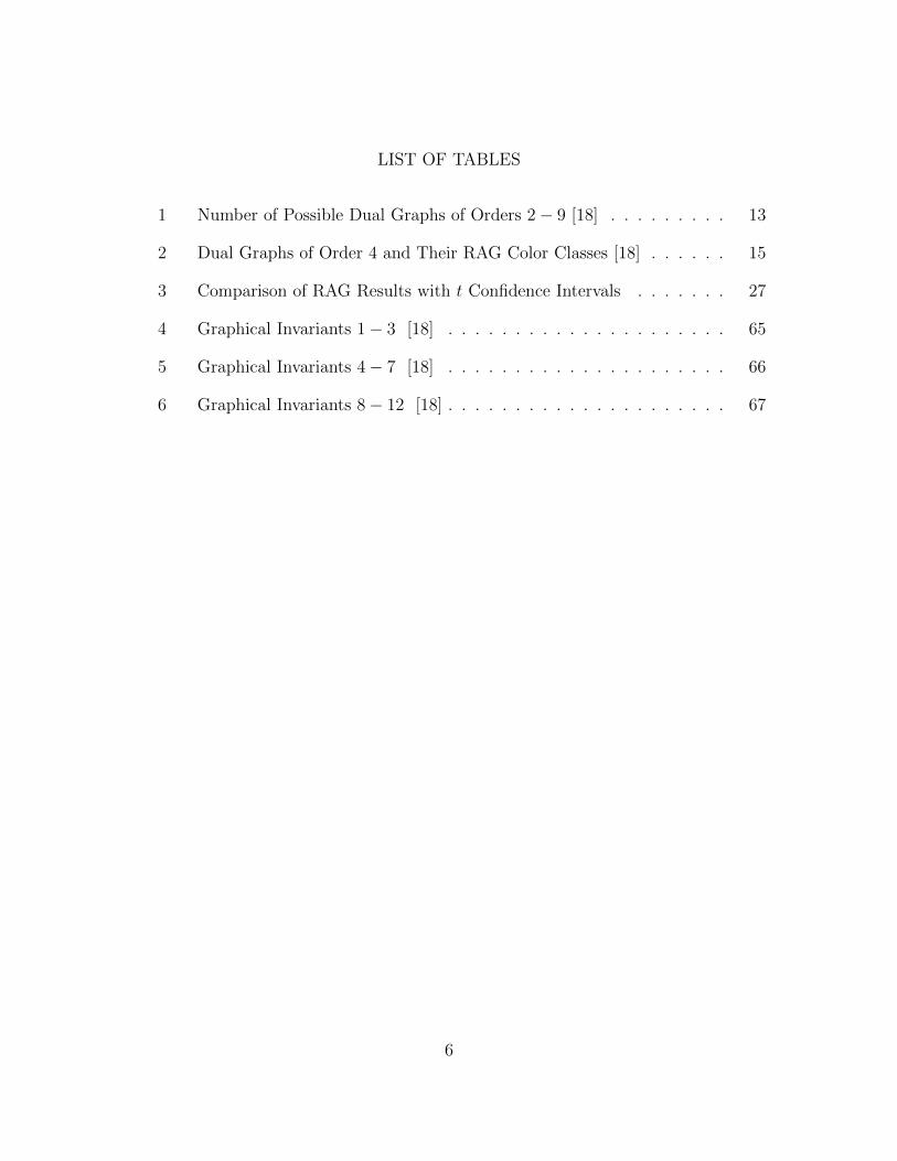
LIST OF TABLES
1 Number of Possible Dual Graphs of Orders 2− 9 [18] . . . . . . . . . 13
2 Dual Graphs of Order 4 and Their RAG Color Classes [18] . . . . . . 15
3 Comparison of RAG Results with t Confidence Intervals . . . . . . . 27
4 Graphical Invariants 1− 3 [18] . . . . . . . . . . . . . . . . . . . . . 65
5 Graphical Invariants 4− 7 [18] . . . . . . . . . . . . . . . . . . . . . 66
6 Graphical Invariants 8− 12 [18] . . . . . . . . . . . . . . . . . . . . . 67
6
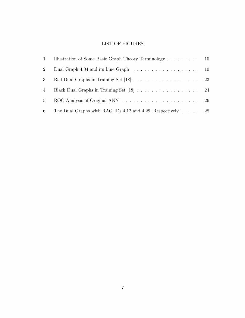
LIST OF FIGURES
1 Illustration of Some Basic Graph Theory Terminology . . . . . . . . . 10
2 Dual Graph 4.04 and its Line Graph . . . . . . . . . . . . . . . . . . 10
3 Red Dual Graphs in Training Set [18] . . . . . . . . . . . . . . . . . . 23
4 Black Dual Graphs in Training Set [18] . . . . . . . . . . . . . . . . . 24
5 ROC Analysis of Original ANN . . . . . . . . . . . . . . . . . . . . . 26
6 The Dual Graphs with RAG IDs 4.12 and 4.29, Respectively . . . . . 28
7

1 BACKGROUND
Until recently, ribonucleic acid (RNA) has been understood to have essentially
one purpose: to facilitate the construction of proteins. The discovery of several
additional types of RNA (non-coding RNA, or ncRNA), whose functions are still
under investigation, has motivated new avenues of research in computational biology.
1.1 RNA
RNA has three basic structures - primary, secondary, and tertiary. The primary
structure is the sequence of nucleotides (adenine (A), cytosine (C), guanine(G), and
uracil (U)). The primary structure folds back on itself to form the secondary struc-
ture, on which we focus in the present research. When the sequence folds, different
combinations of nucleotides (A-U and C-G) bond with each other, forming Watson-
Crick base pairs [10]. In some situations, one of four structures may be formed when
the nucleotides bond; these structures are hairpin loops (“unmatched bases in single-
strand turn region of a helical stem of RNA” [18]), bulges and internal loops (instances
of unmatched base pairs appearing in a helical stem [18]) and junctions (“three or
more helical stems converging to form a closed structure” [18]). The tertiary struc-
ture is formed when secondary structures fold back on themselves. Fortunately, RNA
secondary structures have been found to be indicative of their functions [8]; thus, we
study secondary structures of RNA in this research.
8

1.2 Basic Graph Theory Terminology
In previous research involving RNA secondary structures, the field of mathematics
known as graph theory has been used to model these structures [5, 10, 18, 21]. Before
explaining in more detail how graph theory is used to represent RNA secondary
structures, we give some basic graph theory definitions (for more information, as well
as any undefined notations, see [25]). A graph G is comprised of a vertex set V (G)
and an edge set E(G). We call a graph G with |V (G)| = n a graph of order n. A
graph G with |E(G)| = m has size m. Each edge in E(G) is necessarily paired with
at least one vertex in V (G) such that each edge has two endpoints (note that the edge
may begin and end with the same vertex; in this case, the edge is called a loop) [25].
We represent vertices as dots and edges as lines. It is possible that more than one
edge may have the same pair of vertices as endpoints; in this case, we call the edges
multiple edges. A graph which contains no loops or multiple edges is known as a
simple graph. A graph which may contain both loops and multiple edges is called a
multigraph. It is possible that a graph G may contain vertices which do not serve as
endpoints for any edges in G; in this case, G is disconnected. In the present research,
we consider only connected graphs.
In a graph G, all edges which have the vertex v as an endpoint are called the
incident edges of v. The degree of a vertex v, denoted degG(v), is its number of
incident edges. A vertex u which has only one incident edge is called a leaf, and
degG(u) = 1. For example, let G be the graph with V (G) = {u, v} and E(G) = {uv}.
Then degG(u) = degG(v) = 1. A cycle Ck is a simple graph which contains as many
vertices as it does edges, and which contains vertices V (Ck) = {1, 2, . . . , k}. Then
9

A Simple Graph C5
Vertex
Edge
Tree Graph of Order 5
A Dual Graph (RAG ID 4.13)
A LoopMultiple Edges
Figure 1: Illustration of Some Basic Graph Theory Terminology
E(Ck) = {12, 23, 34, . . . , (k − 1)k, k1}. Notice also that for all vertices v in V (Ck),
degCk(v) = 2. A simple graph which does not contain a cycle is known as a tree [25].
The line graph of a graph G, denoted L(G), is formed by first labeling the edges of
G, then using these labels to label the vertices of L(G). The vertices of L(G) are
adjacent if the edges of the same name in G are adjacent to each other.
Figure 2: Dual Graph 4.04 and its Line Graph
10

1.3 RNA Terminology and the RAG Database ([18])
In [18], both trees and multigraphs (called dual graphs here) are used to represent
RNA secondary structures. In this research, we focus specifically on dual graph
representations of RNA structures. Dual graphs can represent all types of RNA
secondary structures because of their capability to represent pseudoknots, which are a
type of RNA motif formed when nucleotides in a hairpin loop bond with nucleotides
outside the hairpin loop [18]. The simplicity of tree graphs prevents them from
accurately representing RNA pseudoknots. Since dual graphs can represent both trees
and pseudoknots, as well as a third type of RNA motif known as a bridge (“RNAs
with stems connected by a single strand” [18]) which also cannot be represented with
a tree graph, dual graphs are of particular interest. To represent an RNA secondary
structure with a dual graph, we place a vertex everywhere there is a stem (that is,
a structure containing more than one complementary base pair) in the secondary
structure. If the RNA secondary structure contains a hairpin loop, we represent this
with a loop in the form of a circular edge. Bulges and internal loops are represented
by double edges between two vertices. Junctions are also drawn as circular edges,
and may appear in a dual graph as either a set of double edges, a C3, or a C4. [18]
Dual graphs are allowed to have loops and multiple edges, but not required to
have either. There are other constraints placed on dual graphs as well; for example,
every vertex v in a dual graph must have at most degG(v) = 4. Also, dual graphs
contain no leaves. A property of dual graphs noted by Schlick et al. is that if a graph
G is order n, then G has size 2n− 1 [18].
Given the constraints on the number of edges, minimum degree, and maximum
11

degree for a dual graph of order n, it is possible to count the number of possible
structures of dual graphs of order n. Schlick et al. have done this via two different
methods: a probabilistic method [19] and by k − NN clustering [18]. In addition,
Schlick et al. have given the number of RNA motifs (i.e., RNA secondary structures
which correspond to a dual graph in the database) which have been found in na-
ture [18]. Table 1 describes the most recent calculations of the number of possible
dual graphs of orders 2 − 9, as well as the number of RNA motifs which have been
found thus far [18]. The RNA motifs which have been found in nature are colored red
in [18]. The motifs which are thought to be RNA-like by Schlick et al. are colored
blue, and those thought to be not-RNA-like are colored black [18]. These graphs are
ordered by the value of the second-smallest eigenvalue λ2 of their normalized Lapla-
cian matrix [3, 11, 18]. They may be referred to by a label of the form n.r, where
n is the order of G and r is the rank in list of values of λ2 for graphs of this order.
For example, the dual graph whose corresponding value of λ2 is the third largest in
the list of all values of λ2 for order four dual graphs would be labeled 4.3 (note that
for the purposes of the present research, in order to distinguish the label 4.3 from
the label 4.30 in software, we label this graph 4.03). Since there are a total of thirty
dual graphs of order four, the labels range from 4.01 to 4.30. Until November 24,
2010, the RAG classifications for some of the graphs of order four were different; the
present research reflects the current classifications [18, 19]. See Table 2 for a compar-
ison of the previous classifications (denoted “Old Rag Color Class”) and the current
classifications (denoted “New RAG Color Class”) [18, 19].
These motifs are often found in online RNA databases such as [9, 15] and those
12

Table 1: Number of Possible Dual Graphs of Orders 2− 9 [18]
Dual Graph Order Predicted Number of Dual Graphs Number of Motifs Found
2 3 33 8 84 30 175 108 186 494 127 2388 68 12184 39 38595 4
which may be found in [27]. Also, online RNA-folding algorithms have been used
to identify RNA secondary structures (see [27] for a list of these RNA folding al-
gorithms). These algorithms usually fold sequences into secondary structures based
on the resulting free energy of the secondary structure, which has been shown to be
indicative of the structure’s stability [2, 7]. Nonetheless, this is not the only way in
which RNA structure has been predicted. RNA pseudoknots have proven difficult
to predict in some cases (see [17, 26] for more information). Additionally, it has
been shown that graphical invariants, which can be calculated mathematically and
highlight specific properties of graphs, are also indicative of RNA secondary struc-
ture [5, 6, 10]. That is, combinations of invariants which describe red and blue graphs
are different from combinations of invariants which describe black graphs. In [6], a
statistical analysis, combined with graphical invariants involving domination (see 2
for a definition of the domination number of a graph G), showed this result. Also,
in [5], a neural network trained with invariants from known RNA graphs was able
13

to distinguish invariants quantifying RNA-like graphs from those quantifying not-
RNA-like graphs. Also, in [10], a neural network was able to distinguish RNA-like
graphical invariants involving the merging of two trees from those from not-RNA-like
trees; however, in all of these previous studies, RNA tree graphs were studied. In this
paper, we focus on RNA dual graphs. We redefine widely known graphical invariants
for simple graphs so that they may be used with multigraphs, and we use them to
quantify the dual graphs of order four in the RAG database [18].
14
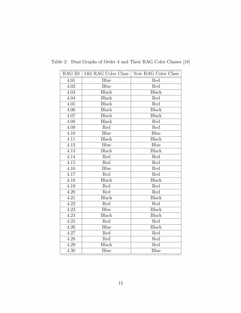
Table 2: Dual Graphs of Order 4 and Their RAG Color Classes [18]
RAG ID Old RAG Color Class New RAG Color Class
4.01 Blue Red4.02 Blue Red4.03 Black Black4.04 Black Red4.05 Black Red4.06 Black Black4.07 Black Black4.08 Black Red4.09 Red Red4.10 Blue Blue4.11 Black Black4.12 Blue Blue4.13 Black Black4.14 Red Red4.15 Red Red4.16 Blue Red4.17 Red Red4.18 Black Black4.19 Red Red4.20 Red Red4.21 Black Black4.22 Red Red4.23 Blue Black4.24 Black Black4.25 Red Red4.26 Blue Black4.27 Red Red4.28 Red Red4.29 Black Red4.30 Blue Blue
15

2 METHODS
2.1 Overview
First, we operationally defined several graphical invariants for use with multi-
graphs. We then calculated these invariants for each of the thirty dual graphs of
order four in the RAG database. Also, we found the line graph of each dual graph
and calculated other invariants of these line graphs (which are simple graphs). We
used a subset of these invariants (for each dual graph or line graph corresponding to
the dual graph) to train an artificial neural network (ANN) to recognize RNA-like
and not-RNA-like sets of invariants. We then classified the RNA-like dual graphs
in the RAG database using the ANN and compared our results with those obtained
by Schlick et al. [18]. Also, using a combinatorial method, we enumerated the dual
graphs of order five.
2.2 Graphical Invariants
We calculated a number of graphical invariants for each order four dual graph
in the RAG database. Many invariants are familiar to graph theorists; however,
others were redefined for use with multigraphs. Several other invariants were derived
from those used often in chemical graph theory [23, 21]. Some invariants were also
calculated using the line graphs of the dual graphs of order four.
We list the definitions of the invariants used with the dual graphs below. Unless
otherwise noted, let G be a dual graph from the RAG database [18]. Also, as it is used
in several invariant definitions, we now define the distance matrix of a dual graph G
16

to be the matrix Di,j where entry dij = dji is the distance from vertex i to vertex j
for vertices i, j ∈ V (G) [23]. If vertex k in V (G) has a loop, then dkk = 1. If there
are n edges between vertices l and m in V (G), then dlm = dml = 1/n.
Dual Graph Invariants
1. [23] Let q be the size of G. Let µ(G) be the number of cycles in G. Define
si =∑n
j=1(dij) to be the sum of all distances in row i of Di,j. Then the Balaban
Index is defined as J(G) = qµ(G)+1
∑ni=1(si)
(−1/2).
2. Let a cycle cii in G be a walk on the vertices of G such that if we begin at vertex
i ∈ V (G), we also end at vertex i. If cii = 121, for example, we count this cycle
once, even if there are multiple ways to traverse that cycle. Then the number
of cycles in G is the number of all unique cycles cii in G. When calculating the
number of cycles, we counted a loop as one cycle. We denote the number of
cycles of G as Nc(G).
3. [25] The diameter of G is commonly defined to be diam(G) = maxi,j∈V (G){dij}.
4. [25] The girth of G is the smallest induced cycle of G, where a cycle is as defined
in 2. We do not count loops in this case. If G has no cycle, we say that the
girth of G is 0 for calculation purposes. (Note that in most instances, an acyclic
graph has girth ∞.) We shall denote the girth of G as g(G).
5. [23] The Wiener number is defined as W (G) = 1/2∑n
i,j=1(dij) where i 6= j.
6. [25] The edge chromatic number of a dual graph G is the size of a proper edge
coloring (i.e., the minimum number of colors required such that no two adjacent
17

edges are the same color) of G. We denote the edge chromatic number of G as
χ′(G).
7. [23] Define the edge degree, denoted D(ei), of an edge ei in E(G) as the number
of edges adjacent to ei. If ej is a loop edge in E(G), then we say that D(ej) = 1.
Then the Platt number F (G) is defined to be F (G) =∑m
i=1D(ei), where m is
the size of G.
8. [1] Define the Randic Index R(G) as R(G) =∑
ij∈E(G)1√
degG(i)degG(j). When
calculating R(G), we count each multiple edge; that is, if there are three edges
ij in E(G), we have a term for each edge ij in the sum R(G).
9. [25] The domination number γ(G) is defined (for a simple graph G) to be the
minimum size of a set S ⊆ V (G) where S is a dominating set if each vertex in
V (G) \ S is adjacent to a member of S. For dual graphs, we define γ(G) to be
the sum of edges incident to vertices in S, where each incident edge is counted
once. Also, if S contains a vertex with a loop edge, we count the loop edge only
once.
10. [25] A matching in G is defined as a set S of edges in G such that if edge ij
is in S, then no other edge in S is incident to either vertex i or vertex j. The
maximum size of a matching is the largest such set S.
We now define the graph invariants we calculated for the line graphs of the dual
graphs of order four. Note that all graphs L(G) are simple graphs.
18

Line Graph Invariants
11. [25] The number of edges of L(G) is simply |E(L(G))|.
12. [25] The maximum degree of L(G) is the maximum number of incident edges of
a vertex i in V (L(G)). We denote the maximum degree of a vertex in V (L(G))
as max{degL(G)(i)}.
13. [25] The vertex chromatic number of L(G) is the size of a proper coloring of
L(G) (i.e., the minimum number of colors required such that no two adjacent
vertices are the same color). The vertex chromatic number of L(G) is denoted
χ(L(G)).
14. [25] A clique in L(G) is “a set of pairwise adjacent vertices” [25]. The clique
number of L(G) is the size of the largest such set in V (L(G)). We denote the
clique number of G as ω(G).
15. [25] The edge chromatic number of L(G), denoted χ′(L(G)), is the size of a
proper edge coloring (i.e., the minimum number of colors required such that no
two adjacent edges are the same color) of L(G).
16. [25] The diameter of L(G) is the maximum distance dij between vertices i, j ∈
V (L(G)). In L(G), we define dij as the minimal number of edges which must
be traversed to reach vertex j from vertex i (or vice-versa). We denote the
diameter of L(G) as diam(L(G)).
17. [25] The girth of L(G) is the smallest induced cycle in L(G), where a cycle is
as defined in Section 1.2. We will denote the girth of L(G) as g(L(G)).
19

18. [25] The edge connectivity of L(G), denoted κ′(L(G)), is the minimum number
of edges which must be removed from E(L(G)) in order for L(G) to become
disconnected.
19. [25] The vertex connectivity of L(G) is the minimum number of vertices which
must be removed from V (L(G)) in order for L(G) to become disconnected.
Vertex connectivity is denoted κ(L(G)).
20. [25] The independence number of L(G) is the size of the largest set of pairwise
nonadjacent vertices (i.e., the size of the largest independent set) in L(G) [25].
We denote the independence number as α(L(G)).
2.3 Artificial Neural Network
Once all invariants were calculated, twelve invariants were chosen for which the
values of the invariant for dual graphs that were red in the RAG database were
noticeably different from those for dual graphs that were black [18]. Other invariants
that were calculated did not appear to discriminate well between red and black dual
graphs, and thus were not included in the analysis. The invariants chosen were as
follows:
1. The Balaban Index of G (J(G))
2. The number of cycles of G (Nc(G))
3. The diameter of G (diam(G))
4. The number of edges of L(G) (|E(L(G))|)
20

5. The maximum degree of a vertex in L(G) (max{degL(G)(i)})
6. The chromatic number of L(G) (χ(L(G)))
7. The girth of G (g(G))
8. The Wiener number of G (W (G))
9. The edge chromatic number of G (χ′(G))
10. The Platt number of G (F (G))
11. The Randic Index of G (R(G))
12. The domination number of G (γ(G))
The values of these invariants were entered into Minitab 14 ([16]). Each of these
invariants was then normalized. We now define normalization for a generic invariant,
call it t. Let R be the label used in the RAG database for each graph of order
four [18]. Denote the value of invariant t for graph R as tR. We first find the mean
xt and standard deviation st of t. We then calculate zt, where
zt =tR − xtst
.
We call zt the normalized value of the invariant t for the dual graph R.
Once each of the twelve invariants were normalized, a vector was created using
the normalized values of the invariants for each dual graph. This vector was of the
form
< zJ(G), zNc(G), zdiam(G), z|E(L(G))|, zmax{degL(G)(i)}, zχ(L(G)), zg(G), zW (G), zχ′(G), zF (G), zR(G), zγ(G) >R .
21
We constructed a vector of this form for each dual graph R in order to enter this vector
into a multi-layer perceptron (MLP) artificial neural network (ANN). The ANN was
trained using a back-propagation algorithm [5, 10, 22]. The ANN used in the present
research contained three layers - an input layer, a hidden layer, and an output layer.
Each layer contains perceptrons, or nodes, which act like artificial neurons in that each
perceptron contains an activation function (or sigmoid function [4]). This design
makes each perceptron similar to an actual neuron in that the activation function
in a perceptron, or artificial neuron, simulates the action potentials in an actual
neuron [4, 22]. In the present research, the input layer contains twelve perceptrons,
one for each graph invariant in the input vector. The hidden layer contains sixteen
perceptrons, and the output layer contains two perceptrons, one for each component
in the output vector < a, b >.
2.3.1 Training Set
To train the ANN, we randomly chose a subset of ten red dual graphs and used
all ten black dual graphs. The purpose of training the ANN is so that it can recognize
graphs which are similar to either the red graphs or the black graphs which are in the
TS. Furthermore, once the ANN is trained, it should classify dual graphs as RNA-like
or not-RNA-like. Thus, in the TS, each of the twenty graphs was denoted by a set of
two vectors. The first vector was a vector of invariant values as defined in Section 2.3,
and the second vector was < 1, 0 > if dual graph R was red in the RAG database,
and < 0, 1 > if dual graph R was black in the RAG database [18]. It should be noted
that no blue dual graphs were used in the TS.
22

4.01 : 4.02 :
4.05 : 4.08 :
4.09 :4.15 :
4.19 : 4.20 :
4.22 : 4.27 :
Figure 3: Red Dual Graphs in Training Set [18]
2.3.2 Classification and Cross-Validation
Once the ANN was trained, the invariant vectors for the remaining ten dual
graphs were given to the ANN for classification. The neural network output was in
the form of a vector < a, b > where 0 ≤ a ≤ 1 and 0 ≤ b ≤ 1. Both a and b are
probabilities; if a is closer to 1, then the dual graph has been classified by the ANN as
RNA-like, and if b is closer to 1, then the dual graph is classified as not-RNA-like. The
23
4.03 : 4.06 :
4.07 : 4.11 :
4.13 :4.18 :
4.21 : 4.23 :
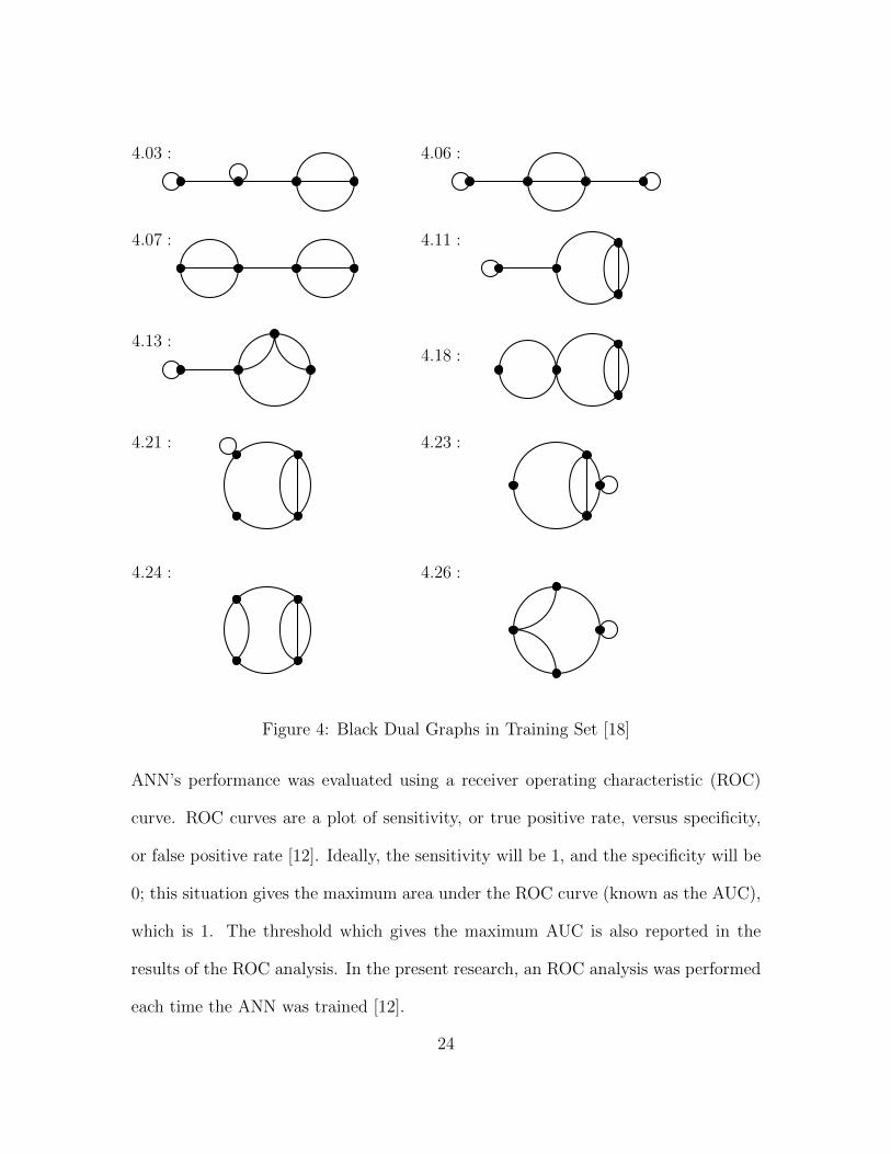
4.24 : 4.26 :
Figure 4: Black Dual Graphs in Training Set [18]
ANN’s performance was evaluated using a receiver operating characteristic (ROC)
curve. ROC curves are a plot of sensitivity, or true positive rate, versus specificity,
or false positive rate [12]. Ideally, the sensitivity will be 1, and the specificity will be
0; this situation gives the maximum area under the ROC curve (known as the AUC),
which is 1. The threshold which gives the maximum AUC is also reported in the
results of the ROC analysis. In the present research, an ROC analysis was performed
each time the ANN was trained [12].
24

To test the results, a method known as cross-validation, or leave-v-out cross val-
idation [5, 10, 20], was implemented. A vector v was removed from the TS, the
network was trained on the new TS, and the dual graphs not in the TS were classified
using the newly trained ANN. This procedure was conducted for each vector v in the
TS; furthermore, each time this was done, three different training lengths were used.
Thus, sixty vectors < a, b > were obtained for each dual graph not in the original
TS. The a values were used to develop a t-confidence interval (computed using the
statistical software Minitab 14 [16]) for the value of a for each dual graph. Also, since
an ROC analysis was performed for each training of the ANN, a confidence interval
was produced for the threshold which gave the maximum AUC [12].
25

3 RESULTS AND DISCUSSION
The TS consisted of ten randomly selected RNA motifs (graphs with RAG ID
4.01, 4.02, 4.05, 4.08, 4.09, 4.15, 4.19, 4.20, 4.22, and 4.27 [18]) and all ten black dual
graphs from the RAG database (graphs 4.03, 4.06, 4.07, 4.11, 4.13, 4.18, 4.21, 4.23
4.24, and 4.26 [18]). First, the neural network was trained using this training set,
and then the vectors corresponding to dual graphs not in the TS were classified by
the network as RNA-like or not-RNA-like. The network converged in approximately
thirty training sessions, with an AUC of 1 and a threshold of 0.05, as shown in the
figure below.
Figure 5: ROC Analysis of Original ANN
26

We then implemented leave-v-out cross-validation, as described above. Each mod-
ified TS was trained for thirty, thirty-two, and thirty-five training sessions. Higher
numbers of training sessions tended to produce a phenomenon known as over-fitting,
in which graphs are not classified correctly simply due to overtraining [13]. For each of
the sixty ROC analyses performed, the AUC was 1. With 95 confidence, the threshold
from the ROC analysis fell between (.030333, .036000). The t-confidence intervals for
the values of a for each dual graph are reported in Table 3.
Table 3: Comparison of RAG Results with t Confidence Intervals
RAG ID RAG Class Mean Value of a Standard Deviation of a t CI for Value of a
4.04 Red 0.99997 0.0000321 (0.999957, 0.999974)4.10 Blue 0.99729 .00342 (0.996404, 0.998173)4.12 Blue 0.5615 0.3175 (0.479504, 0.643549)4.14 Red 0.9414 0.1235 (0.908476, 0.972308)4.16 Red 0.99874 0.00170 (0.998298, 0.999175)4.17 Red 0.9045 0.1596 (0.863227, 0.945673)4.25 Red 0.9120 0.2138 (0.856754, 0.967236)4.28 Red 0.9749 0.1091 (0.946760, 1.003117)4.29 Red 0.6771 0.2908 (0.601964, 0.752204)4.30 Blue 0.99695 0.01454 (0.993194, 1.000707)
Thus, since the threshold for the ROC analysis was so low, our results are similar
to those found by Schlick et al. [18]. It should be noted that the network did not
classify the dual graphs with RAG IDs 4.12 and 4.29 with as much accuracy as the
other dual graphs. In the RAG database, 4.12 is classified as RNA-like, but no actual
RNA secondary structures have yet been found which can be modeled using this dual
graph. The methods used here did classify graph 4.12 as RNA-like, but not to the
27
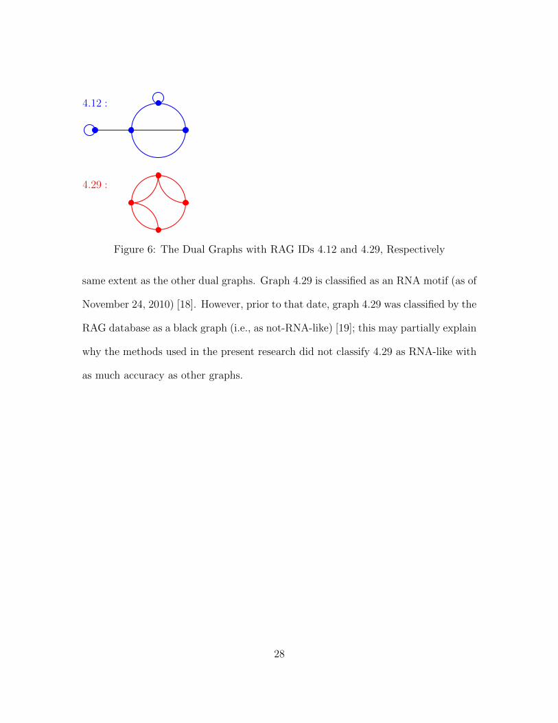
4.12 :
4.29 :
Figure 6: The Dual Graphs with RAG IDs 4.12 and 4.29, Respectively
same extent as the other dual graphs. Graph 4.29 is classified as an RNA motif (as of
November 24, 2010) [18]. However, prior to that date, graph 4.29 was classified by the
RAG database as a black graph (i.e., as not-RNA-like) [19]; this may partially explain
why the methods used in the present research did not classify 4.29 as RNA-like with
as much accuracy as other graphs.
28

4 CONCLUSIONS
The approach taken in the present research followed the design of research pre-
viously conducted [5, 6, 10] in that RNA secondary structures were quantified using
graphical invariants; however, this research is novel in that the definitions of graphical
invariants were modified for use with multigraphs. The invariants used here have been
used in previous research (e.g., [5, 6, 21]) to effectively distinguish between graphical
structures which are RNA-like and those which are not. The approach of training an
artificial neural network to classify dual graphs as RNA-like or not-RNA-like using
graphical invariants was fairly successful, though not as accurate for two of the dual
graphs as perhaps is desired.
Some possible explanations for the less-than-desired accuracy of the classifications
of graphs 4.12 and 4.29 were given in the previous section; however, another possible
reason may be the small size of the training set. There are only thirty dual graphs
of order four. Further research could improve upon the results presented here by
calculating invariants for dual graphs of other orders in order to increase the size of
the training set.
The results from the present work imply that this method, with some improve-
ments, could be quite useful in RNA secondary structure prediction. Another possible
area of application of this research is that of rational drug design [5, 24]. In rational
drug design, the structures of drug receptors are analyzed, and then candidate drugs
are designed based on the structure that would best fit inside the structure of the
receptor [24]. Additionally, the structures of existing drugs/compounds may be ana-
lyzed, and those drugs whose structures are most likely to fit into the drug receptor
29

are tested [24]. Since RNA structure is often indicative of RNA function [8], these
methods could be useful in the rational design of drugs [5].
Also, the results presented here serve as further evidence that it may not be
necessary to consider the free energy (e.g., see [2]) of graphical structures in order
to classify them as RNA-like or not-RNA-like, as none of the invariants used here
depend on the free energy of the graphical structure (for other supporting evidence,
see [5, 6, 10, 21]).
It should also be mentioned that the graphical invariants used in the present
work represent just a subset of the available graphical invariants. Many more have
been defined in the field of mathematical graph theory, as well as in chemical graph
theory (see [23]). Further research may involve the calculation of different graphical
invariants which may be used to quantify RNA graphs and perhaps may allow for
more accurate prediction.
30

BIBLIOGRAPHY
[1] M. Aouchiche and P. Hansen, On a conjecture about the Randic Index, Discrete
Mathematics 307 (2007) 262-265.
[2] L. Childs, Z. Nikoloski, P. May, and D. Walther, Identification and classification
of ncRNA molecules using graph properties, Nucleic Acids Research 37(9) (2009)
1-12.
[3] F. R. K. Chung, Eigenvalues and the Laplacian of a graph, In Lectures on Spectral
Graph Theory, Philadelphia: Chung (1996) 1-22.
[4] C. Gershenson, Artificial Neural Networks for Beginners, [http://arxiv.org/
abs/cs/0308031], (2003). Accessed March 2011.
[5] T. Haynes, D. Knisley, and J. Knisley, Using a Neural Network to Identify Sec-
ondary RNA Structures Quantified by Graphical Invariants, MATCH Commu-
nications in Mathematical and in Computer Chemistry 60 (2008) 277-290.
[6] T. Haynes, D. Knisley, E. Seier, and Y. Zoe, A Quantitative Analysis of Sec-
ondary RNA Structure Using Domination Based Parameters on Trees. BMC
Bioinformatics 7 (2006) 108.
[7] Y. Karklin, R. F. Meraz, and S. R. Holbrook, Classification of non-coding RNA
using graph representations of secondary structure, In PSB Proceedings: 2004
(2004) 1-12.
31
[8] N. Kim, N. Shiffeldrim, H. H. Gan, and T. Schlick, Candidates for novel RNA
topologies, Journal of Molecular Biology 341 (2004) 1129-1144.
[9] N. Kim, J. S. Shin, S. Elmetwaly, H. H. Gan, and T. Schlick, RAGPools: RNA-
As-Graph Pools - A web server for assisting the design of structured RNA pools
for in vitro selection, Structural Bioinformatics, Oxford University Press (2007)
1-2.
[10] D. R. Koessler, D. J. Knisley, J. Knisley, T. Haynes, A Predictive Model for
Secondary RNA Structure Using Graph Theory and a Neural Network, BMC
Bioinformatics 11 (Suppl 6):S21 (2010) 1-10.
[11] E. W. Weisstein, “Laplacian Matrix.” From MathWorld–A Wolfram Web
Resource. [http://mathworld.wolfram.com/LaplacianMatrix.html], (2011).
Accessed April 2011.
[12] T. Lasko, J. Bhagwat, K. Zou and L. Ohno-Machado, The use of receiver op-
erating characteristic curves in biomedical informatics, Journal of Biomedical
Informatics 38 (2005) 404-415.
[13] S. Lawrence, C. Giles and A. Tsoi, Lessons in Neural Network Training: Over-
fitting May be Harder than Expected, Proceedings of the Fourteenth National
Conference on Artificial Intelligence AAAI-97, 540-545 (1997).
[14] Maple 14. (2010). Maplesoft, a division of Waterloo Maple Inc., Waterloo, On-
tario. Maple is a trademark of Waterloo Maple Inc.
32

[15] N. Markham, The Rensselaer bioinformatics web server, [http://mfold.
bioinfo.rpi.edu] (2005). Accessed July 2010.
[16] Minitab Inc. (2003). MINITAB Statistical Software, Release 14 for Windows,
State College, Pennsylvania. MINITAB is a registered trademark of Minitab Inc.
[17] S. Pasquali, H. H. Gan, and T. Schlick, Modular RNA architecture revealed by
computational analysis of existing pseudoknots and ribosomal RNAs, Nucleic
Acids Research 33 (2005) 1384-1398.
[18] T. Schlick, N. Kim, S. Elmetwaly, G. Quarta, J. Izzo, C. Laing, S. Jung, and
A. Iqbal, RAG: RNA-As-Graphs Web Resource, [http://monod.biomath.nyu.
edu/rna/rna.php], (2010). Accessed February 2011.
[19] T. Schlick, H. H. Gan, N. Kim, Y. Xin, G. Quarta, J. S. Shin, and C. Laing,
RAG: RNA-As-Graphs Web Resource (Old version), [http://monod.biomath.
nyu.edu/oldrag/rna.php], (2010). Accessed February 2011.
[20] J. Shao, Linear model selection by cross-validation, J. Am. Statistical Associa-
tion, 88 (1993) 486-494.
[21] W. Shu, X. Bo, Z. Zheng, and S. Wang, A Novel Representation of RNA Sec-
ondary Structure Based on Element-Contact Graphs, BMC Bioinformatics 9:188
(2008).
[22] L. Smith, An Introduction to Neural Networks, [http://www.cs.stir.ac.uk/
~lss/NNIntro/InvSlides.html], (2003). Accessed March 2011.
33
[23] N. Trinajstic, Chemical Graph Theory: Volume II. Boca Raton: CRC Press, Inc.
(1983) 166.
[24] R. Twyman, Rational drug design: Using structural information about drug tar-
gets or their natural ligands as a basis for the design of effective drugs. Copyright
by The Wellcome Trust, [http://genome.wellcome.ac.uk/doc_wtd020912.
html], (2002). Accessed April 2011.
[25] D. B. West, Introduction to Graph Theory, Second Edition, Prentice-Hall, Upper
Saddle River, NJ (2001) 588.
[26] J. Zhao, R. L. Malmberg, and L. Cai, Rapid ab initio prediction of RNA pseu-
doknots via graph tree decomposition, In Proceedings of 6th Workshop on Algo-
rithms for Bioinformatics: 2006 (2006) 1-11.
[27] M. Zuker, Thermodynamics, software and databases for RNA structure, [http:
//www.bioinfo.rpi.edu/zukerm/rna/node3.html], (1998). Accessed February
2011.
34

APPENDICES
Appendix A: Maple 14 Code [14]
In this Appendix, the code used in Maple 14 ([14]) for the multilayer perceptron
artificial neural network used in this research is given verbatim. The reader should
note that comments in Maple are preceded by the symbol #.
The following serves as startup code for the Maple worksheet:
r e s t a r t : with (GraphTheory ) ; with ( p l o t s ) : with ( S t a t i s t i c s ) : with ( LinearAlgebra ) : with ( St r ingToo l s ) :
i n t e r f a c e ( d i s p l a yp r e c i s i o n = 5) ;
i n t e r f a c e ( d i s p l a yp r e c i s i o n =5) ; i n t e r f a c e ( r t a b l e s i z e =22) ;
Below are compiler options, to make the neural network compatible with a Win-
dows Vista operating system.
Neural Network Module
http ://www. cs . s t i r . ac . uk/˜ l s s /NNIntro/ InvS l i d e s . html
Compiler opt ions .
forward := proc ( inputs : : Vector ( datatype = f l o a t [ 8 ] ) , hiddens : : Vector ( datatype = f l o a t [ 8 ] )
, outputs : : Vector ( datatype = f l o a t [ 8 ] ) ,
whi : : Matrix ( datatype = f l o a t [ 8 ] ) , woh : : Matrix ( datatype = f l o a t [ 8 ] ) ,
alpha : : f l o a t [ 8 ] , beta : : Vector ( datatype=f l o a t [ 8 ] ) ,
lbH : : Vector ( datatype=f l o a t [ 8 ] ) , ubH : : Vector ( datatype=f l o a t [ 8 ] ) ,
lbO : : Vector ( datatype=f l o a t [ 8 ] ) , ubO : : Vector ( datatype=f l o a t [ 8 ] ) ,
n i : : pos int , nh : : pos int , no : : pos int , ActOnOutputs : : pos in t )
l o c a l i : : pos int , j : : pos int , acc : : f l o a t [ 8 ] :
f o r i from 1 to nh do
acc :=beta [ i ] :
f o r j from 1 to ni do
acc := acc + whi [ i , j ]∗ inputs [ j ] :
end do :
hiddens [ i ] := lbH [ i ] + (ubH [ i ] − lbH [ i ] ) /( exp(−(ubH [ i ] − lbH [ i ] ) ∗acc )+1) :
end do :
35

f o r i from 1 to no do
acc := 0 . 0 :
f o r j from 1 to nh do
acc := acc + woh [ i , j ]∗ hiddens [ j ] :
end do :
i f ( ActOnOutputs = 2) then
outputs [ i ] := lbO [ i ] + (ubO[ i ] − lbO [ i ] ) /( exp(−(ubO[ i ] − lbO [ i ] ) ∗acc )+1) :
e l s e
outputs [ i ] := acc :
end i f :
end do :
re turn true ;
end proc :
backprop := proc ( l rn input : : Vector ( datatype = f l o a t [ 8 ] ) ,
l rnoutput : : Vector ( datatype = f l o a t [ 8 ] ) ,
hiddens : : Vector ( datatype = f l o a t [ 8 ] ) ,
outputs : : Vector ( datatype = f l o a t [ 8 ] ) ,
whi : : Matrix ( datatype = f l o a t [ 8 ] ) ,
woh : : Matrix ( datatype = f l o a t [ 8 ] ) ,
pwhi : : Matrix ( datatype = f l o a t [ 8 ] ) ,
pwoh : : Matrix ( datatype = f l o a t [ 8 ] ) ,
d e l t o : : Vector ( datatype=f l o a t [ 8 ] ) ,
de l th : : Vector ( datatype=f l o a t [ 8 ] ) ,
alpha : : f l o a t [ 8 ] , BetaDecay : : f l o a t [ 8 ] ,
beta : : Vector ( datatype = f l o a t [ 8 ] ) ,
betachange : : Vector ( datatype = f l o a t [ 8 ] ) ,
lbH : : Vector ( datatype=f l o a t [ 8 ] ) , ubH : : Vector ( datatype=f l o a t [ 8 ] ) ,
lbO : : Vector ( datatype=f l o a t [ 8 ] ) , ubO : : Vector ( datatype=f l o a t [ 8 ] ) ,
N : : f l o a t [ 8 ] , M: : f l o a t [ 8 ] ,
n i : : pos int , nh : : pos int , no : : pos int , ActOnOutputs : : pos int , TrainThresholds : :
po s in t )
l o c a l i : : pos int , j : : pos int , k : : pos int , incErro r : : f l o a t [ 8 ] , acc : : f l o a t [ 8 ] , tmp : : f l o a t [ 8 ] , change : :
f l o a t [ 8 ] ;
##Calcu la te e r r o r and de l t o
incError :=0 . 0 :
f o r i from 1 to no by 1 do
36
i ncError := incError + 0 .5∗ ( outputs [ i ]− l rnoutput [ i ] ) ∗( outputs [ i ]− l rnoutput [ i ] ) :
i f (ActOnOutputs = 2) then
de l t o [ i ] :=( outputs [ i ]−lbO [ i ] ) ∗(ubO[ i ] − outputs [ i ] ) ∗( l rnoutput [ i ]−outputs [ i ] ) :
e l s e
de l t o [ i ] := l rnoutput [ i ]−outputs [ i ] :
end i f :
end do :
##Calcu la te de l th
f o r j from 1 to nh do
acc := 0 . 0 :
f o r k from 1 to no do
acc := acc + de l t o [ k ]∗woh [ k , j ] :
end do :
de l th [ j ] := ( hiddens [ j ]− lbH [ j ] ) ∗(ubH [ j ]−hiddens [ j ] ) ∗acc :
end do :
## Update woh
f o r j from 1 to nh do
f o r k from 1 to no do
change := de l t o [ k ] ∗ hiddens [ j ] :
woh [ k , j ] := woh [ k , j ] + N∗change + M∗pwoh [ k , j ] :
pwoh [ k , j ] := change :
end do :
end do :
##update whi
f o r i from 1 to ni do
f o r j from 1 to nh do
change := de l th [ j ]∗ l r n input [ i ] :
whi [ j , i ] := whi [ j , i ] + N∗change + M∗pwhi [ j , i ] :
pwhi [ j , i ] := change :
end do :
end do :
##update beta
i f ( TrainThresholds=2) then
f o r j from 1 to nh do
beta [ j ] := BetaDecay∗beta [ j ] + N∗ de l th [ j ] + M∗betachange [ j ] :
betachange [ j ] := de l th [ j ] :
end do :
end i f :
37

re turn incError ;
end proc :
#try
cforward :=Compiler :−Compile ( forward ) ;
cbackprop :=Compiler :−Compile ( backprop ) ;
#catch :
# cforward := forward ;
# cbackprop :=backprop ;
# Maplets :−Examples:−Alert ( ”Compiling Fa i l ed . Using i n t e rp r e t ed v e r s i on s in s t ead . ” ) ;
#end try ;
The following code creates the artificial neural network and defines commands for
the ROC analysis.
Creates the neura l network :
MakeANN := proc ( n i : : pos int , no : : po s in t )
l o c a l nh , tmp , ActOnOut , thebetadecay , ThThresh , themomentum , anneal ing , annea l i ng s ca l e r , bds ,
t h e l r n r a t e ;
nh := ni ∗no ;
t ry
i f ( hasopt ion ( [ args [ 3 . . − 1 ] ] , ’ hiddens ’ , ’ tmp ’ ) or hasopt ion ( [ args [ 3 . . − 1 ] ] , ’ Hiddens ’ , ’ tmp ’ ) or
hasopt ion ( [ args [ 3 . . − 1 ] ] , ’ hidden ’ , ’ tmp ’ ) or hasopt ion ( [ args [ 3 . . − 1 ] ] , ’ Hidden ’ , ’ tmp ’ ) )
then
i f ( type (tmp , ’ pos int ’ ) ) then
nh := tmp ;
e l s e
e r r o r
end i f :
end i f :
ActOnOut := 1 :
i f ( hasopt ion ( [ args [ 3 . . − 1 ] ] , ’ ActivationOnOutputs ’ , ’ tmp ’ ) ) then
i f (tmp = f a l s e or tmp = 0) then ActOnOut := 0 e l s e e r r o r end i f :
end i f :
ThThresh := 1 :
i f ( hasopt ion ( [ args [ 3 . . − 1 ] ] , ’ ThresholdTraining ’ , ’ tmp ’ ) ) then
i f (tmp = true or tmp = 1) then ThThresh := 1 e l s e e r r o r end i f :
38

end i f :
t h e l r n r a t e := 0 . 5 :
i f ( hasopt ion ( [ args [ 3 . . − 1 ] ] , ’ LearningRate ’ , ’ tmp ’ ) ) then
i f (0 < tmp and tmp <= 1) then th e l r n r a t e := tmp e l s e e r r o r end i f :
end i f :
thebetadecay := 1 :
i f ( hasopt ion ( [ args [ 3 . . − 1 ] ] , ’ ThresholdScal ing ’ , ’ tmp ’ ) ) then
i f (0 < tmp and tmp <= 1) then thebetadecay := tmp e l s e e r r o r end i f :
end i f :
themomentum := 0 . 0 :
i f ( hasopt ion ( [ args [ 3 . . − 1 ] ] , ’Momentum’ , ’ tmp ’ ) ) then
i f (0 <= tmp and tmp <= 1) then themomentum := tmp e l s e e r r o r end i f :
end i f :
#Annealing i s ” i n t e r n a l ” v ia the th r e sho ld s
annea l ing := 0 . 0 :
i f ( hasopt ion ( [ args [ 3 . . − 1 ] ] , ’ Annealing ’ , ’ tmp ’ ) ) then
i f (0 <= tmp ) then annea l ing := tmp end i f :
end i f :
a nn ea l i n g s c a l e r := 0 . 0 :
i f ( hasopt ion ( [ args [ 3 . . − 1 ] ] , ’ Anneal ingScaler ’ , ’ tmp ’ ) ) then
i f (0 <= tmp ) then annea l i n g s c a l e r := tmp end i f :
end i f :
bds := [ 0 . 0 , 1 . 0 , 0 . 0 , 1 . 0 ] :
i f ( hasopt ion ( [ args [ 3 . . − 1 ] ] , ’ Bounds ’ , ’ tmp ’ ) or hasopt ion ( [ args [ 3 . . − 1 ] ] , ’ bounds ’ , ’ tmp ’ ) ) then
i f ( type (tmp , ’ l i s t ( numeric ) ’ ) ) then bds := tmp end i f :
end i f :
catch :
e r r o r cat (” Inva l i d Option . Val id opt ions are ’ ActivationOnOutputs ’ = true / f a l s e , ’ Annealing ’
= x>=0, ’ Anneal ingScaler ’ = x>= 0 ” ,
” ’ hiddens ’ = po s i t i v e i n t e g e r , ’Momentum’= 0<=x<=1, ’ Thresholds ’ = numeric , ’
ThresholdScal ing ’ = 0<x<=1 ” ,
” or ’ ThresholdTraining ’= true / f a l s e . ” ) ;
end try :
re turn module ( )
39
l o c a l l e a rn ra t e , numints , numouts , numhids , inputs , hiddens , outputs , de l to , delth , whi , woh
, forward , backprop , lbH , ubH , lbO , ubO,
outputsbetas , h iddensbetas , e r r s , cnt , f , TrainingSet , Patterns , Complements ,
WeightsUpdated , momentum, Annealing , betachange ,
Anneal ingScaler , prevwhi , prevwoh , ActivateOutputs , pttns , preds , betadecay ,
ThresholdTraining , alpha ;
export I n i t i a l i z e , Forward , BackProp , C la s s i f y , Get ,
Set , SetAlpha , SetBetas , SetLearningRate , SetThresho ldSca l ing , SetThresholdTraining ,
SetThresholds , SetActivationOnOutputs ,
SetMomentum , SetAnnealing , SetAnneal ingSca ler , Train , AddPattern , RemovePattern ,
CreateComplement ,
ResetPatterns , PredictComplements , Errors , Tra in ingResults , ShowPatterns , SetBounds ;
g l oba l cforward , cbackprop ;
l e a r n r a t e := convert ( the l rn ra t e , ’ f l o a t [ 8 ] ’ ) :
momentum := convert ( themomentum , ’ f l o a t [ 8 ] ’ ) :
numints := ni : #This i s the number o f inputs in each pattern
numouts:=no : #This i s the number o f outputs
numhids:=nh :
WeightsUpdated := f a l s e :
e r r s := [ ] :
cnt := 0 :
ActivateOutputs := ActOnOut :
ThresholdTraining := ThThresh :
Annealing := convert ( anneal ing , ’ f l o a t [ 8 ] ’ ) :
Annea l ingSca le r := convert ( annea l i ng s ca l e r , ’ f l o a t [ 8 ] ’ ) :
# I n i t i a l i z e ar rays
inputs := Vector [ column ] ( numints , datatype=f l o a t [ 8 ] ) :
hiddens := Vector [ column ] ( numhids , datatype=f l o a t [ 8 ] ) :
outputs := Vector [ column ] ( numouts , datatype=f l o a t [ 8 ] ) :
#the ” de lta ’ s ”
de l t o := Vector [ column ] ( numouts , datatype=f l o a t [ 8 ] ) :
de l th := Vector [ column ] ( numhids , datatype=f l o a t [ 8 ] ) :
#weights in the form whi [ hidden ] [ input ] and woh [ outputs ] [ hidden ]
whi := Matrix ( numhids , numints , datatype=f l o a t [ 8 ] ) : #Hidden l ay e r weights
woh := Matrix ( numouts , numhids , datatype=f l o a t [ 8 ] ) : #Output l ay e r weights
40

prevwhi := Matrix ( numhids , numints , datatype=f l o a t [ 8 ] ) : #Hidden l ay e r momentum tmpvar
prevwoh := Matrix ( numouts , numhids , datatype=f l o a t [ 8 ] ) : #Output l ay e r momentum tmpvar
#Def ine th r e sho ld s
h iddensbetas := Vector [ column ] ( numhids , datatype=f l o a t [ 8 ] , f i l l =0.0) :
betachange := Vector [ column ] ( numhids , datatype=f l o a t [ 8 ] , f i l l =0.0) :
#Def ine Bounds
lbH := Vector [ column ] ( numhids , datatype=f l o a t [ 8 ] , f i l l =min ( bds [ 1 ] , bds [ 2 ] ) ) :
ubH := Vector [ column ] ( numhids , datatype=f l o a t [ 8 ] , f i l l =max( bds [ 1 ] , bds [ 2 ] ) ) :
lbO := Vector [ column ] ( numhids , datatype=f l o a t [ 8 ] , f i l l =min ( bds [ 3 ] , bds [ 4 ] ) ) :
ubO := Vector [ column ] ( numhids , datatype=f l o a t [ 8 ] , f i l l =max( bds [ 3 ] , bds [ 4 ] ) ) :
##Act ivat ion i s o f the form :
f := entryv −> lbO [ 1 ] + (ubO [ 1 ] − lbO [ 1 ] ) /( exp(−(ubO [ 1 ] − lbO [ 1 ] ) ∗ entryv )+1) ;
alpha := convert ( 1 . 0 , ’ f l o a t [ 8 ] ’ ) :
betadecay := convert ( thebetadecay , ’ f l o a t [ 8 ] ’ ) :
Get := proc ( )
l o c a l item , r e f :
i f ( nargs > 0 ) then r e f := args [ 1 ]
e l s e
re turn [ ” l e a r n r a t e ” = lea rn ra t e , ”momentum” = momentum, ”numints”=numints , ”numhids”
=numhids , ”numouts” = numouts ,
”whi” =whi , ”woh”=woh , ” alpha”=alpha , ”bounds” =[lbH [ 1 ] , ubH [ 1 ] , lbO [ 1 ] , ubO
[ 1 ] ] , ” hiddenbetas ” = hiddensbetas ,
” betachange ” = betachange , ” t h r e s h o l d s c a l i n g ” = betadecay , ”
t h r e s ho l d t r a i n i n g ” = ThresholdTraining ,
” annea l ing ” = Annealing , ” t r a i n i n g s e t ” = TrainingSet , ” pat te rns ” =Patterns ,
”complements” = Complements ] :
end i f :
item := Str ingToo l s :−LowerCase ( convert ( r e f , ’ s t r i ng ’ ) ) :
i f ( item = ” l e a r n r a t e ” ) then return l e a r n r a t e end i f :
i f ( item = ”momentum” ) then return momentum end i f :
i f ( item = ”numints” ) then return numints end i f :
i f ( item = ”numouts” ) then return numouts end i f :
i f ( item = ”numhids” ) then return numhids end i f :
i f ( item = ”whi” ) then return whi end i f :
i f ( item = ”woh” ) then return woh end i f :
i f ( item = ”alpha” ) then return alpha end i f :
41

i f ( item = ”bounds” ) then return [ lbH [ 1 ] , ubH [ 1 ] , lbO [ 1 ] , ubO [ 1 ] ] end i f :
i f ( item = ”hiddenbetas ” ) then return hiddensbetas end i f :
i f ( item = ”betachange ” ) then return betachange end i f :
i f ( item = ” th r e s h o l d s c a l i n g ”) then return betadecay end i f :
i f ( item = ” th r e s ho l d t r a i n i n g ”) then return ThresholdTraining end i f :
i f ( item = ” act iva t i ononoutput s ”) then return ActivateOutputs end i f :
i f ( item = ” annea l ing ”) then return Annealing end i f :
i f ( item = ” annea l i n g s c a l e r ”) then return Annealing end i f :
i f ( item = ” e r r s ” ) then return e r r s end i f :
i f ( item = ”cnt ” ) then return cnt end i f :
i f ( item = ” f ” ) then return f end i f :
i f ( item = ” f p l o t ” ) then return
p lo t ( f ,−10/(ubH[1]− lbH [ 1 ] ) . . 1 0 / ( ubH[1]− lbH [ 1 ] ) , c o l o r=blue , t i t l e =”Act ivat ion Function
: Threshold=0”, t i t l e f o n t =[TIMES,BOLD, 1 4 ] )
end i f :
i f ( item = ” t r a i n i n g s e t ” ) then return Train ingSet end i f :
i f ( item = ” pat te rns ” ) then return Patterns end i f :
i f ( item = ”complements” ) then return Complements end i f :
end proc :
Set := proc ( r e f )
l o c a l item , tmp :
try
i f ( type ( re f , ’ equation ’ ) ) then
item := Str ingToo l s :−LowerCase ( convert ( l h s ( r e f ) , ’ s t r i ng ’ ) ) :
tmp := rhs ( r e f ) :
e l s e
item := Str ingToo l s :−LowerCase ( convert ( r e f , ’ s t r i ng ’ ) ) :
tmp := args [ 2 ] :
end :
catch :
e r r o r ” Inva l i d input in to Set . ”
end try :
p r in t (tmp , type (tmp , ’ l i s t ’ ) , whattype (tmp) ) ;
i f ( item = ” l e a r n r a t e ” ) then return SetLearningRate (tmp) end i f :
i f ( item = ”alpha” ) then return SetAlpha (tmp) end i f :
i f ( item = ”bounds” ) then return SetBounds (tmp) end i f :
i f ( item = ”momentum” ) then return SetMomentum(tmp) end i f :
i f ( item = ” th r e s ho l d t r a i n i n g ” ) then return SetThreholdTraining (tmp) end i f :
i f ( item = ” th r e s h o l d s c a l i n g ” ) then return SetThresho ldSca l ing (tmp) end i f :
i f ( item = ” thr e sho ld s ” ) then return SetThresholds (tmp) end i f :
42

i f ( item = ” act iva t i ononoutput s ” ) then return SetActivationOnOutputs (tmp) end i f :
i f ( item = ” annea l ing ” ) then return SetAnneal ing (tmp) end i f :
i f ( item = ” annea l i n g s c a l e r ” ) then return SetAnnea l ingSca le r (tmp) end i f :
r e turn FAIL
end proc :
SetAlpha :=proc ( va l : : numeric )
l o c a l tmp :
tmp:=alpha :
alpha := convert ( val , ’ f l o a t [ 8 ] ’ ) :
r e turn tmp :
end proc :
SetBounds :=proc ( va l )
l o c a l tmp , i :
tmp:=[ lbH [ 1 ] , ubH [ 1 ] , lbO [ 1 ] , ubO [ 1 ] ] :
i f ( nops ( va l ) = 2) then
f o r i from 1 to numhids do
lbH [ i ] , ubH [ i ] := min ( va l [ 1 ] , va l [ 2 ] ) , max( va l [ 1 ] , va l [ 2 ] ) :
end do :
f o r i from 1 to numouts do
lbO [ i ] , ubO [ i ] := min ( va l [ 1 ] , va l [ 2 ] ) , max( va l [ 1 ] , va l [ 2 ] ) :
end do :
e l i f ( nops ( va l ) = 4) then
f o r i from 1 to numhids do
lbH [ i ] , ubH [ i ] := min ( va l [ 1 ] , va l [ 2 ] ) , max( va l [ 1 ] , va l [ 2 ] ) :
end do :
f o r i from 1 to numouts do
lbO [ i ] , ubO [ i ] := min ( va l [ 3 ] , va l [ 4 ] ) , max( va l [ 3 ] , va l [ 4 ] ) :
end do :
e l s e
e r r o r (” L i s t o f bounds must have e i t h e r 2 or 4 e n t r i e s ”)
end i f :
r e turn tmp :
end proc :
SetThresholds :=proc ( va l )
#Option o f a number , a l i s t that i s d i s t r i bu t ed ac ro s s hiddens , then betas un t i l
exhausted , or two l i s t s in which the
#f i r s t changes hiddens and the second outputs , but only the numeric e n t r i e s do so
43

l o c a l ind , i :
i f ( type ( val , ’ numeric ’ ) ) then
f o r i from 1 to numhids do
hiddensbetas [ i ] := va l :
end do :
f o r i from 1 to numouts do
outputsbetas [ i ] := va l :
end do :
re turn true :
e l i f ( type ( val , ’ l i s t ( l i s t ) ’ ) ) then
f o r i from 1 to nops ( va l [ 1 ] ) do
i f ( i <= numhids and type ( va l [ 1 ] [ i ] , ’ numeric ’ ) ) then
hiddensbetas [ i ] := va l [ 1 ] [ i ] :
end i f :
end do :
f o r i from 1 to nops ( va l [ 2 ] ) do
i f ( i <= numouts and type ( va l [ 2 ] [ i ] , ’ numeric ’ ) ) then
outputsbetas [ i ] := va l [ 2 ] [ i ] :
end i f :
end do :
e l i f ( type ( val , ’ l i s t ( numeric ) ’ ) ) then
whi le ( ind < nops ( va l ) and ind <= numhids + numouts ) do
try
i f ( ind <= numhids ) then
hiddensbetas [ ind ] := va l [ ind ] :
e l s e
outputsbetas [ ind−numhids ] := va l [ ind ] :
end i f :
catch :
break :
end try :
ind := ind + 1 :
end do :
re turn ind :
e l s e
re turn f a l s e :
end i f :
end proc :
SetLearningRate :=proc ( va l : : numeric )
44
l o c a l tmp :
tmp:= l e a r n r a t e :
i f ( va l > 0 ) then
l e a r n r a t e := convert ( val , ’ f l o a t [ 8 ] ’ ) ;
end i f :
r e turn l e a r n r a t e :
end proc :
SetThresho ldSca l ing :=proc ( va l : : numeric )
l o c a l tmp :
tmp:=betadecay :
i f ( va l > 0 .0 and va l <= 1.0 ) then
betadecay := convert ( val , ’ f l o a t [ 8 ] ’ ) ;
end i f :
r e turn tmp :
end proc :
SetMomentum:=proc ( va l : : numeric )
l o c a l tmp :
tmp:=momentum :
i f ( va l > 0 .0 and va l <= 1.0 ) then
momentum := convert ( val , ’ f l o a t [ 8 ] ’ ) ;
end i f :
r e turn tmp :
end proc :
SetAnneal ing :=proc ( va l : : numeric )
l o c a l tmp :
tmp:=Annealing :
i f ( va l >= 0.0 ) then
Annealing := convert ( val , ’ f l o a t [ 8 ] ’ ) ;
end i f :
r e turn tmp :
end proc :
SetAnnea l ingSca le r :=proc ( va l : : numeric )
l o c a l tmp :
tmp:=Annea l ingSca le r :
i f ( va l >= 0.0 ) then
Annea l ingSca le r := convert ( val , ’ f l o a t [ 8 ] ’ ) ;
end i f :
r e turn tmp :
45

end proc :
SetThresholdTrain ing :=proc ( va l : : boolean )
l o c a l tmp :
tmp := ThresholdTraining :
i f ( va l ) then ThresholdTraining := 1 e l s e ThresholdTraining := 0 end i f :
r e turn tmp ;
end proc :
SetActivationOnOutputs :=proc ( va l : : boolean )
l o c a l tmp :
tmp := ActivateOutputs :
i f ( va l ) then ActivateOutputs := 1 e l s e ActivateOutputs := 0 end i f :
r e turn tmp ;
end proc :
I n i t i a l i z e :=proc (maxamt) #i n i t a l i z e weights to smal l random va lues with mag
l o c a l i , h , o :
f o r h from 1 to numhids do
hiddensbetas [ h ] :=( rand ( ) ∗10ˆ(−11)−5)∗maxamt :
f o r i from 1 to numints do
whi [ h , i ] :=( rand ( ) ∗10ˆ(−11)−5)∗maxamt :
prevwhi [ h , i ] := whi [ h , i ] :
end do :
end do :
f o r o from 1 to numouts do
outputsbetas [ o ] :=( rand ( ) ∗10ˆ(−11)−5)∗maxamt :
f o r h from 1 to numhids do
woh [ o , h ] :=( rand ( ) ∗10ˆ(−11)−5)∗maxamt :
prevwoh [ o , h ] :=woh [ o , h ] :
end do :
end do :
cnt := 0 :
WeightsUpdated := true :
e r r s : = [ ] :
end proc :
Forward := proc ( inpt : : Vector )
l o c a l i n p f l 8 ;
i n p f l 8 := Vector ( inpt , datatype=f l o a t [ 8 ] ) :
c forward ( inp f l 8 , hiddens , outputs , whi , woh , alpha , hiddensbetas , lbH , ubH , lbO , ubO,
46

numints , numhids , numouts , ActivateOutputs+1) :
re turn outputs ;
end proc :
#Def ine the forward func t i on
C l a s s i f y :=proc ( inpat : : Vector )
LinearAlgebra [ Transpose ] ( Forward ( inpat ) ) :
end proc :
BackProp:=proc ( l rn input : : Vector , l rnoutput : : Vector )
l o c a l tmpLinpt , tmpLoutp , annl , annlseq , threshva lues , i ;
Forward ( l rn input ) :
tmpLinpt := Vector ( l rn input , datatype=f l o a t [ 8 ] ) ;
tmpLoutp := Vector ( lrnoutput , datatype=f l o a t [ 8 ] ) ;
WeightsUpdated := true :
i f ( Annealing >= 0.01 ) then
i f ( Annealing <= 1 ) then
annl := f l o o r ( Annealing ∗( numhids + numouts ) ) :
e l s e
annl := min ( numhids+numouts , f l o o r ( Annealing ) ) :
end i f :
annlseq := combinat [ randperm ] ( [ seq ( i , i =1. . numhids+numouts ) ] ) [ 1 . . annl ] ;
f o r i in annlseq do
i f ( i <= numhids ) then
hiddensbetas [ i ] := Annea l ingSca le r ∗hiddensbetas [ i ] :
e l s e
outputsbetas [ i−numhids+1] := Annea l ingSca le r ∗ outputsbetas [ i−numhids+1] :
end i f :
end do :
end i f :
cbackprop ( tmpLinpt , tmpLoutp , hiddens , outputs , whi , woh , prevwhi , prevwoh , de l to , delth , alpha ,
betadecay ,
hiddensbetas , betachange , lbH , ubH , lbO , ubO, l ea rn ra t e ,momentum,
numints , numhids , numouts , ActivateOutputs , ThresholdTraining+1) :
47

end proc :
##Training Set Algorithms
Patterns : = [ ] :
AddPattern := proc ( inp , oup )
l o c a l inpt , oupt , a t t r ;
a t t r := ”” :
hasopt ion ( [ args [ 3 . . − 1 ] ] , ’ a t t r i bu t e s ’ , ’ a t t r ’ ) :
inpt := Vector ( convert ( inp , ’ l i s t ’ ) , o r i e n t a t i o n=column ) : #pr in t ( inpt ) ;
oupt := Vector ( convert ( oup , ’ l i s t ’ ) , o r i e n t a t i o n=column ) : #pr in t ( oupt ) ;
i f ( LinearAlgebra :−Dimensions ( inpt ) = numints and LinearAlgebra :−Dimensions ( oupt ) =
numouts ) then
Patterns := [ Patterns [ ] , [ inpt , oupt , a t t r ] ] :
Tra in ingSet := [ seq ( i , i =1. . nops ( Patterns ) ) ] :
t rue :
e l s e
f a l s e :
end i f :
end proc :
RemovePattern := proc ( PatIndex : : pos in t )
i f ( PatIndex <= nops ( Patterns ) ) then
Patterns := [ Patterns [ 1 . . PatIndex −1] , Patterns [ PatIndex +1 . . −1 ] ] :
t rue :
e l s e
f a l s e :
end i f :
end proc :
ShowPatterns := proc ( )
Patterns ;
end proc :
ResetPatterns := proc ( )
Patterns :=[ ] :
48

Train ingSet := [ ] :
Complements := [ ] :
end proc :
CreateComplement := proc ( amt ) #amt i s the proport ion or number to use to put in to the
complement
l o c a l tmp :
i f (0 <= amt and amt < 1 ) then
tmp := f l o o r (amt ∗ nops ( Patterns ) ) :
e l i f ( 1 <= amt and amt < nops ( Patterns ) ) then
tmp := amt :
end i f :
Tra in ingSet := { seq ( i , i =1. . nops ( Patterns ) ) } :
Complements := { seq ( combinat [ randperm ] ( Tra in ingSet ) [ j ] , j =1. . tmp) } :
Tra in ingSet := convert ( Tra in ingSet minus Complements , ’ l i s t ’ ) ;
Complements := convert (Complements , ’ l i s t ’ ) :
r e turn ’TrainBy ’ , TrainingSet , ’ ValidateWith ’ , Complements ;
end proc :
Train := proc (NumberOfReps : : pos int , amt := 0 )
l o c a l In i tValue , c l s , t e r r , Ind i ce s , TSI , VSI , i , n , esum , tsum , v , tmp ;
i f (0 <= amt and amt < 1 ) then
tmp := f l o o r (amt ∗ nops ( Tra in ingSet ) ) :
e l i f ( 1 <= amt and amt < nops ( Tra in ingSet ) ) then
tmp := amt :
end i f :
## tmp i s number o f pat te rns to p a r t i t i o n in to ” t e s t aga in s t ” s e t
i f ( tmp >= nops ( Tra in ingSet ) ) then e r r o r ( ”Test s e t o f s i z e ” , tmp ,” i s l a r g e r than
t r a i n i n g s e t . ” ) end i f :
t e r r := [ ] :
TSI := combinat [ randperm ] ( Tra in ingSet ) :
VSI := TSI [ 1 . . tmp ] :
TSI := TSI [ tmp+1. .−1] :
f o r n from 1 to NumberOfReps do
Ind i c e s := combinat [ randperm ] ( TSI ) :
esum :=0:
49
pttns := [ ] :
preds := [ ] :
f o r i in I nd i c e s do
v:=Patterns [ i ] :
esum := esum + BackProp (v [ 1 ] , v [ 2 ] ) :
pttns := [ pttns [ ] , v [ 2 ] [ 1 ] ] ;
preds := [ preds [ ] , outputs [ 1 ] ] :
end do :
tsum := 0 :
f o r i in VSI do
v:=Patterns [ i ] :
c l s :=Forward (v [ 1 ] ) :
tsum := tsum + LinearAlgebra :−VectorNorm ( c l s−v [ 2 ] ) :
end do :
cnt := cnt+1:
e r r s := [ e r r s [ ] , esum ] :
t e r r := [ t e r r [ ] , tsum ] :
end do :
re turn er r s , t e r r ;
end proc :
Errors := ( ) −> e r r s ;
Tra in ingResu l t s := proc ( binary := true )
l o c a l v , i , err , c l s ;
e r r := 0 :
pttns : = [ ] :
preds : = [ ] :
f o r i in Tra in ingSet do
v:=Patterns [ i ] :
c l s :=Forward (v [ 1 ] ) :
pttns := [ pttns [ ] , v [ 2 ] [ 1 ] ] ;
preds := [ preds [ ] , outputs [ 1 ] ] :
e r r := e r r + LinearAlgebra :−VectorNorm ( c l s−v [ 2 ] ) :
end do :
i f ( b inary ) then
50

re turn e r r /nops ( Patterns ) , ROCanalysis ( pttns , preds )
e l s e
re turn e r r /nops ( Patterns ) , pttns , preds ;
end i f :
end proc :
PredictComplements := proc ( binary := true )
l o c a l v , i , err , c l s ;
e r r := 0 :
pttns : = [ ] :
preds : = [ ] :
f o r i in Complements do
v:=Patterns [ i ] :
c l s :=Forward (v [ 1 ] ) :
pttns := [ pttns [ ] , v [ 2 ] [ 1 ] ] ;
preds := [ preds [ ] , outputs [ 1 ] ] :
e r r := e r r + LinearAlgebra :−VectorNorm ( c l s−v [ 2 ] ) :
end do :
i f ( b inary ) then
return e r r /nops ( Patterns ) , ROCanalysis ( pttns , preds )
e l s e
re turn e r r /nops ( Patterns ) , pttns , preds ;
end i f :
end proc :
end module :
end proc :
SaveNet := proc (nnme) # ANNfN i s op t i ona l 2nd argument
l o c a l ANNfN, Args , NetName ;
ANNfN := NULL:
NetName := convert (nnme , ’ s t r i ng ’ ) :
i f ( nargs>1 and type ( args [ 2 ] , ’ s t r i ng ’ ) ) then
ANNfN := args [ 2 ] :
Args := args [ 3 . . − 1 ] :
e l s e
ANNfN := Maplets [ U t i l i t i e s ] [ GetFi le ] ( ’ t i t l e ’ = ”Save as . . . ” , f i l ename = cat (NetName , ” .mnn”) ,
’ d i r e c to ry ’ = cu r r en td i r ( ) , approvecapt ion=”Save ” , approvecheck=f a l s e ,
51

’ f i l e f i l t e r ’ = ”mnn” , ’ f i l t e r d e s c r i p t i o n ’ = ”Maple Neural Network ”) :
Args := args [ 2 . . − 1 ] :
end i f :
use St r ingToo l s in
i f ( LowerCase ( SubString (ANNfN,−4..−1) )<> ” .mnn” and SubString (ANNfN,−1..−1) <> ” ” ) then
ANNfN := cat (ANNfN, ” .mnn”) :
end i f :
end use :
save parse (NetName) , ANNfN;
end proc :
LoadNet := proc ( )
l o c a l ANNfN ;
ANNfN := NULL:
i f ( nargs>0 and type ( args [ 1 ] , ’ s t r i ng ’ ) ) then
ANNfN := args [ 1 ] :
e l s e
ANNfN := Maplets [ U t i l i t i e s ] [ GetFi le ] ( ’ t i t l e ’ = ”Open Neural Network ” ,
’ d i r e c to ry ’ = cu r r en td i r ( ) , approvecapt ion=”Open” ,
’ f i l e f i l t e r ’ = ”mnn” , ’ f i l t e r d e s c r i p t i o n ’ = ”Maple Neural Network ”) :
end i f :
read ANNfN;
end proc :
ROCanalysis := proc ( Actual , Pred icted )
l o c a l k , PosValues , NegValues , PosNum, NegNum, thresh , threshs , tmin , tmax , npts ,
PosInd , NegInd , BestThresh , opt , p lt , tmp , d i s t , ROC , AUC ;
i f ( nops ( Pred icted ) <> nops ( Actual ) ) then
e r r o r ”Actual and Pred icted are l i s t s o f corresponding va lues ”
end i f :
PosValues := [ ] :
NegValues := [ ] :
npts := 10 : #Later we ’ l l make t h i s an opt ion
f o r k from 1 to nops ( Actual ) do
i f ( Actual [ k ] = 1 ) then
52

PosValues := [ PosValues [ ] , Pred icted [ k ] ] :
e l s e
NegValues := [ NegValues [ ] , Pred icted [ k ] ] :
end i f :
end do :
PosValues := so r t ( PosValues ) ;
PosNum := nops ( PosValues ) :
PosValues := queue [ new ] ( PosValues [ ] ) :
NegValues := so r t ( NegValues ) :
NegNum := nops ( NegValues ) :
NegValues := queue [ new ] ( NegValues [ ] ) :
##Eliminate dup l i c a t e th r e sho ld s by conver t ing to a s e t
tmax := max( Pred icted ) ;
tmin := min ( Pred icted ) :
th r e shs := convert ( Predicted , ’ set ’ ) :
th r e shs := so r t ( convert ( Predicted , ’ l i s t ’ ) ) :
ROC := [ [ 1 , 1 ] ] :
BestThresh := [ 2 , 0 , [ 1 , 1 ] ] :
f o r thresh in thre shs do ##from tmin to tmax by e v a l f ( ( tmax−tmin ) /npts ) do
whi le ( ( not queue [ empty ] ( PosValues ) ) and queue [ f r on t ] ( PosValues ) <= thresh ) do
queue [ dequeue ] ( PosValues ) :
end do :
whi le ( ( not queue [ empty ] ( NegValues ) ) and queue [ f r on t ] ( NegValues ) <= thresh ) do
queue [ dequeue ] ( NegValues ) :
end do :
tmp := [ e v a l f ( queue [ l ength ] ( NegValues ) /NegNum) , e v a l f ( queue [ l ength ] ( PosValues ) /PosNum) ] :
### debugging
#pr in t ( thresh , queue [ l ength ] ( NegValues ) , queue [ l ength ] ( PosValues ) , tmp) ;
d i s t := ev a l f ( s q r t (tmp [ 1 ] ˆ 2 + (tmp[2]−1) ˆ2) ) :
i f ( d i s t < BestThresh [ 1 ] ) then
BestThresh := [ d i s t , thresh , tmp ] :
end i f :
ROC := [ ROC [ ] , tmp ] :
end do :
AUC := add ( abs ( ( ROC [ k ] [ 1 ] − ROC [ k+1 ] [ 1 ] ) ) ∗( ROC [ k ] [ 2 ]+ ROC [ k+1 ] [ 2 ] ) , k=1 . . ( nops ( ROC
53

)−1) ) /2 ;
p l t := p l o t s [ d i sp l ay ] (
p l o t s [ l i s t p l o t ] ( ROC , co l o r=blue ) ,
p l o t s [ l i s t p l o t ] ( ROC , s t y l e=point , symbol=s o l i d c i r c l e , c o l o r=blue ) ,
p l o t s [ l i s t p l o t ] ( [ [ 0 , 0 ] , [ 1 , 1 ] ] , s t y l e=l in e , c o l o r=grey ) ,
p l o t s [ po in tp l o t ] ( BestThresh [ 3 ] , s t y l e=point , symbol=s o l i d c i r c l e , c o l o r=green ,
symbols i ze=20) ,
p l o t s [ t e x tp l o t ] ( [ BestThresh [ 3 ] [ 1 ] , BestThresh [ 3 ] [ 2 ] ,
cat (” (” , s p r i n t f (”%0.2 f ” , BestThresh [ 3 ] [ 1 ] ) , ” ,” , s p r i n t f (”%0.2 f ” , BestThresh
[ 3 ] [ 2 ] ) ,” ) ”) ] ,
f ont=[TIMES,ROMAN, 1 4 ] , a l i g n =[BELOW,RIGHT] ) ,
axes=boxed , l a b e l s =[” S p e c i f i c i t y ” ,” S e n s i t i v i t y ” ] , l a b e l d i r e c t i o n s =[ hor i zonta l ,
v e r t i c a l ] ,
f ont = [TIMES,ROMAN, 1 4 ] , view = [ 0 . . 1 , 0 . . 1 ] , t i t l e = cat (”ROC Curve : \n Threshold =
” ,
s p r i n t f (”%0.2 f ” , BestThresh [ 2 ] ) , ” , AUC = ” , s p r i n t f (”%0.2 f ” , AUC ) )
) ;
opt :=”none ” :
hasopt ion ( [ args [ 3 . . − 1 ] ] , ’ output ’ , ’ opt ’ ) :
opt := Str ingToo l s :−UpperCase ( convert ( opt , ’ s t r i ng ’ ) ) :
i f ( opt = ”SOLUTIONMODULE” ) then
return
module ( )
l o c a l auc , best , roc , c l s t ;
export AUC, ROCplot , BestThreshold , ROC ;
best := BestThresh [ 2 ] :
c l s t := BestThresh [ 3 ] :
auc := AUC ;
roc := ROC ;
AUC := ( ) −> auc ;
BestThreshold := ( ) −> best ;
ROC := ( ) −> roc ;
ROCplot := ( ) −> p l t ;
end module ;
e l i f ( opt = ”AUC”) then
return AUC
e l i f ( opt = ”ROC”) then
return ROC
e l i f ( opt = ”OOP” or opt = ”BESTTHRESHOLD” or opt = ”BEST” ) then
54

re turn BestThresh [ 2 ]
e l i f ( opt = ”LOCATION”) then
return BestThresh [ 3 ]
e l s e
re turn p l t
end i f :
end proc :
rnd :=rand ( 1 . . 1 0 0 ) :
ROCanalysis ( [ seq (0 , i =1. .200) , seq (1 , i =1. .200) ] , [ seq ( rnd ( ) ∗ i , i =1. .400) ] ) ;
ROCanalysis ( [ seq (0 , i =1. .200) , seq (1 , i =1. .200) ] , [ seq ( rnd ( ) , i =1. .400) ] , output=”so lut ionmodule ”) ;
r r :=%;
r r :−AUC() :
r r :−ROCplot ( ) ;
The following code executes the neural network, defines the original TS, executesthirty training sessions, and performs an ROC analysis.
RNANet : F i r s t Training Set ( de sc r ibed above )
#Red in TS : 4 . 01 , 4 . 02 , 4 . 05 , 4 . 08 , 4 . 09 , 4 . 15 , 4 . 19 , 4 . 20 , 4 . 22 , and 4 .27
RNANet := MakeANN(12 ,2 , hiddens=16, Momentum = 0 . 1 ) ;
Tra in ingSet
:={ [ <2.70149 ,0.03195 ,2.77377 ,−2.50280 ,−2.95843 ,−2.61216 ,−3.39110 ,2.82848 ,−1.67967 ,−1.92803 ,2.51898 ,
−0.56106> , <1 ,0>] ,
[ <1.88125 ,0.03195 ,1.57931 ,−1.70407 ,−1.83483 ,−1.26081 ,−0.21145 ,1.61636 ,−1.67967 ,−1.49315 ,1.43993 ,0.32389 > ,
<1 ,0>] ,
[<0.78996 ,−0.93611 ,−0.01338 ,−0.50599 ,0.41236 ,0.09054 ,−0.21145 ,−0.20182 ,−0.05366 ,−0.62340 ,−0.43680 ,1.20885> ,
<1 ,0>] ,
[ <0.75765 ,0 .03195 ,0 .38485 ,−0.50599 ,−0.71124 ,0 .09054 ,−0.21145 ,0 .10121 ,−0.05366 ,−0.62340 ,0 .64225 ,0 .32389 > ,
<1 ,0>] ,
[ <1.55979 ,0.03195 ,0.38485 ,−0.90535 ,−0.71124 ,0.09054 ,−0.21145 ,1.01030 ,−0.05366 ,−1.05827 ,1.63153 ,−0.56106 > ,
<1 ,0>] ,
[ <−0.35361 ,0.03195 ,−0.80960 ,−0.10663 ,0.41236 ,0.09054 ,−0.21145 ,0.10121 ,−0.05366 ,−0.18852 ,0.14292 ,−0.56106 > ,
<1 ,0>] ,
[ <0.13570 ,0 .03195 ,0 .38485 ,−0.90535 ,−0.71124 ,−1.26081 ,2 .96820 ,1 .31333 ,−1.67967 ,−1.05827 ,1 .03037 ,0 .32389 > ,
<1 ,0>] ,
[ <−0.30520 ,0.03195 ,0.38485 ,−0.10663 ,−0.71124 ,−1.26081 ,−0.21145 ,0.10121 ,−0.05366 ,−0.62340 ,0.36088 ,1.20885 > ,
<1 ,0>] ,
[ <−0.76353 ,1.00000 ,0.38485 ,−0.10663 ,−0.71124 ,−1.26081 ,1.37838 ,0.40424 ,−1.67967 ,−0.18852 ,0.36088 ,0.32389 > ,
<1 ,0>] ,
[ <−1.04899 ,1.00000 ,−0.80960 ,1.09145 ,1.53596 ,1.44189 ,−0.21145 ,−1.11091 ,1.57236 ,1.98587 ,−1.31934 ,−0.56106 > ,
<1 ,0>] ,
[ <1.59418 ,−0.93611 ,1.18108 ,−1.30471 ,−0.71124 ,0.09054 ,−0.21145 ,1.01030 ,−0.05366 ,−1.05827 ,0.64225 ,0.32389 > ,
<0 ,1>] ,
55

[ <0.99270 ,−0.93611 ,1.18108 ,−0.50599 ,−0.71124 ,0.09054 ,−0.21145 ,0.60624 ,−0.05366 ,−0.62340 ,0.91380 ,−0.56106 > ,
<0 ,1>] ,
[<0.50827 ,−1.90416 ,−0.41137 ,−0.10663 ,1.53596 ,0.09054 ,−0.21145 ,−0.80788 ,−0.05366 ,−0.18852 ,−1.20768 ,1.20885> ,
<0 ,1>] ,
[ <−0.36349 ,−0.93611 ,0 .38485 ,0 .29273 ,0 .41236 ,1 .44189 ,−0.21145 ,0 .30321 ,1 .57236 ,0 .24636 ,−0.07548 ,−1.44602 > ,
<0 ,1>] ,
[ <−0.57366 ,0 .03195 ,0 .38485 ,0 .69209 ,0.41236 ,1 .44189 ,−0.21145 ,−0.20182 ,1 .57236 ,0 .68124 ,−0.14694 ,−0.56106 > ,
<0 ,1>] ,
[ <−0.63643 ,−0.93611 ,0.38485 ,1.09145 ,1.53596 ,1.44189 ,−0.21145 ,−0.90891 ,1.57236 ,1.11611 ,−1.31934 ,−0.56106 > ,
<0 ,1>] ,
[ <−0.47360 ,−0.93611 ,0.38485 ,0.29273 ,0.41236 ,1.44189 ,−0.21145 ,−0.20182 ,−0.05366 ,0.24636 ,−0.53015 ,1.20885 > ,
<0 ,1>] ,
[ <−0.88702 ,0 .03195 ,0 .38485 ,1 .09145 ,0.41236 ,0 .09054 ,−0.21145 ,−0.20182 ,1 .57236 ,1 .11611 ,−0.60161 ,−0.56106 > ,
<0 ,1>] ,
[ <−0.70762 ,−0.93611 ,−0.80960 ,0.69209 ,0.41236 ,0.09054 ,−0.21145 ,−1.11091 ,−0.05366 ,0.68124 ,−1.15453 ,2.09381 > ,
<0 ,1>] ,
[ <−0.56804 ,0.03195 ,−0.80960 ,0.29273 ,−0.71124 ,0.09054 ,−0.21145 ,−0.80788 ,−0.05366 ,0.24636 ,−0.43680 ,1.20885 > ,
<0 ,1>]};
nops ( Tra in ingSet ) ;
f o r TS in Train ingSet do
RNANet:−AddPattern (TS [ 1 ] ,TS [ 2 ] )
end do :
RNANet:−ShowPatterns ( ) ;
RNANet:−Get ( f p l o t ) ;
RNANet:− I n i t i a l i z e ( 0 . 1 ) ;
RNANet:−Train (30) ;
p l o t s [ l i s t p l o t ](%) ;
RNANet:−Tra in ingResu l t s ( ) ;% [ 2 ] ;
The following code tells the neural network to classify graph invariant vectors forthe dual graphs not in the TS.
RNANet:−C l a s s i f y
( <1.07417 ,0.03195 ,0.38485 ,−0.90535 ,−0.71124 ,−1.26081 ,−0.21145 ,0.40424 ,−1.67967 ,−1.05827 ,0.36088 ,0.32389 >)
; %[1]+%[2] ; #Red4 .04
RNANet:−C l a s s i f y
( <−0.04566 ,0.03195 ,0.38485 ,−1.30471 ,−0.71124 ,−1.26081 ,1.37838 ,1.31333 ,−0.05366 ,−1.05827 ,1.43993 ,−1.44602 >)
; %[1]+%[2] ; #Blue4 .10
RNANet:−C l a s s i f y
( <−0.31290 ,0 .03195 ,0 .38485 ,−0.10663 ,0 .41236 ,0 .09054 ,1 .37838 ,0 .40424 ,1 .57236 ,−0.18852 ,0 .59714 ,−0.56106 >)
; %[1]+%[2] ; #Blue4 .12
RNANet:−C l a s s i f y
( <−1.24837 ,3.90416 ,−2.00406 ,1.89018 ,0.41236 ,0.09054 ,1.37838 ,−1.11091 ,−0.05366 ,1.98587 ,−1.18133 ,−1.44602 >)
56
; %[1]+%[2] ; #Blue4 .30
RNANet:−C l a s s i f y
( <0.14688 ,0.03195 ,−0.80960 ,0.29273 ,0.41236 ,0.09054 ,−0.21145 ,−1.11091 ,−0.05366 ,0.24636 ,−0.60161 ,0.32389 >)
; %[1]+%[2] ; #Red4 .14
RNANet:−C l a s s i f y
( <−0.37170 ,0.03195 ,−0.80960 ,−0.10663 ,0.41236 ,0.09054 ,−0.21145 ,0.10121 ,−0.05366 ,−0.18852 ,0.18758 ,−0.56106 >)
; %[1]+%[2] ; #Red4 .16
RNANet:−C l a s s i f y
( <−0.58348 ,0.03195 ,−0.80960 ,0.29273 ,0.41236 ,0.09054 ,−0.21145 ,−0.50485 ,−0.05366 ,0.24636 ,−0.43680 ,−0.56106 >)
; %[1]+%[2] ; #Red4 .17
RNANet:−C l a s s i f y
( <−0.96015 ,1.00000 ,−0.80960 ,1.09145 ,0.41236 ,1.44189 ,−0.21145 ,−0.50485 ,−0.05366 ,0.68124 ,−0.43680 ,−1.44602 >)
; %[1]+%[2] ; #Red4 .25
RNANet:−C l a s s i f y
( <−1.06683 ,1.00000 ,−0.80960 ,1.49081 ,1.53596 ,0.09054 ,−0.21145 ,−1.11091 ,−0.05366 ,1.55099 ,−1.20768 ,−0.56106 >)
;%[1 ]+%[2 ] ; #Red4 .28
RNANet:−C l a s s i f y
( <−0.86698 ,0.03195 ,−2.00406 ,1.09145 ,0.41236 ,0.09054 ,−0.21145 ,−1.71697 ,−0.05366 ,1.11611 ,−1.18133 ,2.09381 >)
; %[1]+%[2] ; #Red4 .29
The code below performs the method of leave-v-out cross-validation. The codegiven here is when the first vector, corresponding to dual graph 4.01, is removed fromthe TS. First, the network is trained thirty times, and the non-TS dual graphs areclassified; then, the network is trained thirty-two times, and the non-TS dual graphsare classified; finally, the network is trained thirty-five times, and the non-TS dualgraphs are classified. The code below may be repeated for other adjusted trainingsets in which vectors for dual graphs other than 4.01 are removed from the TS.
Training Se s s i on 1 : Leave−v−out Cross Va l idat ion
#In t h i s t r a i n i n g s e s s i on , the f i r s t vec tor i s l e f t out o f the o r i g i n a l TS . Thus , we l a b e l t h i s
new TS as TS1 .
RNANet1 := MakeANN(12 ,2 , hiddens=16, Momentum = 0 . 1 ) ;
Tra in ingSet1 :={
[ <1.88125 ,0.03195 ,1.57931 ,−1.70407 ,−1.83483 ,−1.26081 ,−0.21145 ,1.61636 ,−1.67967 ,−1.49315 ,1.43993 ,0.32389 > ,
<1 ,0>] ,
[<0.78996 ,−0.93611 ,−0.01338 ,−0.50599 ,0.41236 ,0.09054 ,−0.21145 ,−0.20182 ,−0.05366 ,−0.62340 ,−0.43680 ,1.20885> ,
<1 ,0>] ,
[ <0.75765 ,0 .03195 ,0 .38485 ,−0.50599 ,−0.71124 ,0 .09054 ,−0.21145 ,0 .10121 ,−0.05366 ,−0.62340 ,0 .64225 ,0 .32389 > ,
<1 ,0>] ,
[ <1.55979 ,0.03195 ,0.38485 ,−0.90535 ,−0.71124 ,0.09054 ,−0.21145 ,1.01030 ,−0.05366 ,−1.05827 ,1.63153 ,−0.56106 > ,
<1 ,0>] ,
[ <−0.35361 ,0.03195 ,−0.80960 ,−0.10663 ,0.41236 ,0.09054 ,−0.21145 ,0.10121 ,−0.05366 ,−0.18852 ,0.14292 ,−0.56106 > ,
<1 ,0>] ,
[ <0.13570 ,0 .03195 ,0 .38485 ,−0.90535 ,−0.71124 ,−1.26081 ,2 .96820 ,1 .31333 ,−1.67967 ,−1.05827 ,1 .03037 ,0 .32389 > ,
57

<1 ,0>] ,
[ <−0.30520 ,0.03195 ,0.38485 ,−0.10663 ,−0.71124 ,−1.26081 ,−0.21145 ,0.10121 ,−0.05366 ,−0.62340 ,0.36088 ,1.20885 > ,
<1 ,0>] ,
[ <−0.76353 ,1.00000 ,0.38485 ,−0.10663 ,−0.71124 ,−1.26081 ,1.37838 ,0.40424 ,−1.67967 ,−0.18852 ,0.36088 ,0.32389 > ,
<1 ,0>] ,
[ <−1.04899 ,1.00000 ,−0.80960 ,1.09145 ,1.53596 ,1.44189 ,−0.21145 ,−1.11091 ,1.57236 ,1.98587 ,−1.31934 ,−0.56106 > ,
<1 ,0>] ,
[ <1.59418 ,−0.93611 ,1.18108 ,−1.30471 ,−0.71124 ,0.09054 ,−0.21145 ,1.01030 ,−0.05366 ,−1.05827 ,0.64225 ,0.32389 > ,
<0 ,1>] ,
[ <0.99270 ,−0.93611 ,1.18108 ,−0.50599 ,−0.71124 ,0.09054 ,−0.21145 ,0.60624 ,−0.05366 ,−0.62340 ,0.91380 ,−0.56106 > ,
<0 ,1>] ,
[<0.50827 ,−1.90416 ,−0.41137 ,−0.10663 ,1.53596 ,0.09054 ,−0.21145 ,−0.80788 ,−0.05366 ,−0.18852 ,−1.20768 ,1.20885> ,
<0 ,1>] ,
[ <−0.36349 ,−0.93611 ,0 .38485 ,0 .29273 ,0 .41236 ,1 .44189 ,−0.21145 ,0 .30321 ,1 .57236 ,0 .24636 ,−0.07548 ,−1.44602 > ,
<0 ,1>] ,
[ <−0.57366 ,0 .03195 ,0 .38485 ,0 .69209 ,0.41236 ,1 .44189 ,−0.21145 ,−0.20182 ,1 .57236 ,0 .68124 ,−0.14694 ,−0.56106 > ,
<0 ,1>] ,
[ <−0.63643 ,−0.93611 ,0.38485 ,1.09145 ,1.53596 ,1.44189 ,−0.21145 ,−0.90891 ,1.57236 ,1.11611 ,−1.31934 ,−0.56106 > ,
<0 ,1>] ,
[ <−0.47360 ,−0.93611 ,0.38485 ,0.29273 ,0.41236 ,1.44189 ,−0.21145 ,−0.20182 ,−0.05366 ,0.24636 ,−0.53015 ,1.20885 > ,
<0 ,1>] ,
[ <−0.88702 ,0 .03195 ,0 .38485 ,1 .09145 ,0.41236 ,0 .09054 ,−0.21145 ,−0.20182 ,1 .57236 ,1 .11611 ,−0.60161 ,−0.56106 > ,
<0 ,1>] ,
[ <−0.70762 ,−0.93611 ,−0.80960 ,0.69209 ,0.41236 ,0.09054 ,−0.21145 ,−1.11091 ,−0.05366 ,0.68124 ,−1.15453 ,2.09381 > ,
<0 ,1>] ,
[ <−0.56804 ,0.03195 ,−0.80960 ,0.29273 ,−0.71124 ,0.09054 ,−0.21145 ,−0.80788 ,−0.05366 ,0.24636 ,−0.43680 ,1.20885 > ,
<0 ,1>]};
nops ( Tra in ingSet1 ) ;
f o r TS in Train ingSet1 do
RNANet1:−AddPattern (TS [ 1 ] ,TS [ 2 ] )
end do :
RNANet1:−ShowPatterns ( ) ;
RNANet1:−Get ( f p l o t ) ;
RNANet1:− I n i t i a l i z e ( 0 . 1 ) ;
RNANet1:−Train (30) ;
p l o t s [ l i s t p l o t ](%) ;
RNANet1:−Tra in ingResu l t s ( ) ;% [ 2 ] ;
RNANet1:−C l a s s i f y
( <2.70149 ,0.03195 ,2.77377 ,−2.50280 ,−2.95843 ,−2.61216 ,−3.39110 ,2.82848 ,−1.67967 ,−1.92803 ,2.51898 ,−0.56106 >)
; %[1]+%[2] ; #Red4 .01 ( l e f t out o f t h i s TS)
RNANet1:−C l a s s i f y
58

( <1.07417 ,0.03195 ,0.38485 ,−0.90535 ,−0.71124 ,−1.26081 ,−0.21145 ,0.40424 ,−1.67967 ,−1.05827 ,0.36088 ,0.32389 >)
; %[1]+%[2] ; #Red4 .04
RNANet1:−C l a s s i f y
( <−0.04566 ,0.03195 ,0.38485 ,−1.30471 ,−0.71124 ,−1.26081 ,1.37838 ,1.31333 ,−0.05366 ,−1.05827 ,1.43993 ,−1.44602 >)
; %[1]+%[2] ; #Blue4 .10
RNANet1:−C l a s s i f y
( <−0.31290 ,0 .03195 ,0 .38485 ,−0.10663 ,0 .41236 ,0 .09054 ,1 .37838 ,0 .40424 ,1 .57236 ,−0.18852 ,0 .59714 ,−0.56106 >)
; %[1]+%[2] ; #Blue4 .12
RNANet1:−C l a s s i f y
( <−1.24837 ,3.90416 ,−2.00406 ,1.89018 ,0.41236 ,0.09054 ,1.37838 ,−1.11091 ,−0.05366 ,1.98587 ,−1.18133 ,−1.44602 >)
; %[1]+%[2] ; #Blue4 .30
RNANet1:−C l a s s i f y
( <0.14688 ,0.03195 ,−0.80960 ,0.29273 ,0.41236 ,0.09054 ,−0.21145 ,−1.11091 ,−0.05366 ,0.24636 ,−0.60161 ,0.32389 >)
; %[1]+%[2] ; #Red4 .14
RNANet1:−C l a s s i f y
( <−0.37170 ,0.03195 ,−0.80960 ,−0.10663 ,0.41236 ,0.09054 ,−0.21145 ,0.10121 ,−0.05366 ,−0.18852 ,0.18758 ,−0.56106 >)
; %[1]+%[2] ; #Red4 .16
RNANet1:−C l a s s i f y
( <−0.58348 ,0.03195 ,−0.80960 ,0.29273 ,0.41236 ,0.09054 ,−0.21145 ,−0.50485 ,−0.05366 ,0.24636 ,−0.43680 ,−0.56106 >)
; %[1]+%[2] ; #Red4 .17
RNANet1:−C l a s s i f y
( <−0.96015 ,1.00000 ,−0.80960 ,1.09145 ,0.41236 ,1.44189 ,−0.21145 ,−0.50485 ,−0.05366 ,0.68124 ,−0.43680 ,−1.44602 >)
; %[1]+%[2] ; #Red4 .25
RNANet1:−C l a s s i f y
( <−1.06683 ,1.00000 ,−0.80960 ,1.49081 ,1.53596 ,0.09054 ,−0.21145 ,−1.11091 ,−0.05366 ,1.55099 ,−1.20768 ,−0.56106 >)
;%[1 ]+%[2 ] ; #Red4 .28
RNANet1:−C l a s s i f y
( <−0.86698 ,0.03195 ,−2.00406 ,1.09145 ,0.41236 ,0.09054 ,−0.21145 ,−1.71697 ,−0.05366 ,1.11611 ,−1.18133 ,2.09381 >)
; %[1]+%[2] ; #Red4 .29
#Now we w i l l use a second t r a i n i n g length on Train ingSet1 :
RNANet2 := MakeANN(12 ,2 , hiddens=16, Momentum = 0 . 1 ) ;
Tra in ingSet1 :={
[ <1.88125 ,0.03195 ,1.57931 ,−1.70407 ,−1.83483 ,−1.26081 ,−0.21145 ,1.61636 ,−1.67967 ,−1.49315 ,1.43993 ,0.32389 > ,
<1 ,0>] ,
[<0.78996 ,−0.93611 ,−0.01338 ,−0.50599 ,0.41236 ,0.09054 ,−0.21145 ,−0.20182 ,−0.05366 ,−0.62340 ,−0.43680 ,1.20885> ,
<1 ,0>] ,
[ <0.75765 ,0 .03195 ,0 .38485 ,−0.50599 ,−0.71124 ,0 .09054 ,−0.21145 ,0 .10121 ,−0.05366 ,−0.62340 ,0 .64225 ,0 .32389 > ,
<1 ,0>] ,
[ <1.55979 ,0.03195 ,0.38485 ,−0.90535 ,−0.71124 ,0.09054 ,−0.21145 ,1.01030 ,−0.05366 ,−1.05827 ,1.63153 ,−0.56106 > ,
<1 ,0>] ,
[ <−0.35361 ,0.03195 ,−0.80960 ,−0.10663 ,0.41236 ,0.09054 ,−0.21145 ,0.10121 ,−0.05366 ,−0.18852 ,0.14292 ,−0.56106 > ,
<1 ,0>] ,
59

[ <0.13570 ,0 .03195 ,0 .38485 ,−0.90535 ,−0.71124 ,−1.26081 ,2 .96820 ,1 .31333 ,−1.67967 ,−1.05827 ,1 .03037 ,0 .32389 > ,
<1 ,0>] ,
[ <−0.30520 ,0.03195 ,0.38485 ,−0.10663 ,−0.71124 ,−1.26081 ,−0.21145 ,0.10121 ,−0.05366 ,−0.62340 ,0.36088 ,1.20885 > ,
<1 ,0>] ,
[ <−0.76353 ,1.00000 ,0.38485 ,−0.10663 ,−0.71124 ,−1.26081 ,1.37838 ,0.40424 ,−1.67967 ,−0.18852 ,0.36088 ,0.32389 > ,
<1 ,0>] ,
[ <−1.04899 ,1.00000 ,−0.80960 ,1.09145 ,1.53596 ,1.44189 ,−0.21145 ,−1.11091 ,1.57236 ,1.98587 ,−1.31934 ,−0.56106 > ,
<1 ,0>] ,
[ <1.59418 ,−0.93611 ,1.18108 ,−1.30471 ,−0.71124 ,0.09054 ,−0.21145 ,1.01030 ,−0.05366 ,−1.05827 ,0.64225 ,0.32389 > ,
<0 ,1>] ,
[ <0.99270 ,−0.93611 ,1.18108 ,−0.50599 ,−0.71124 ,0.09054 ,−0.21145 ,0.60624 ,−0.05366 ,−0.62340 ,0.91380 ,−0.56106 > ,
<0 ,1>] ,
[<0.50827 ,−1.90416 ,−0.41137 ,−0.10663 ,1.53596 ,0.09054 ,−0.21145 ,−0.80788 ,−0.05366 ,−0.18852 ,−1.20768 ,1.20885> ,
<0 ,1>] ,
[ <−0.36349 ,−0.93611 ,0 .38485 ,0 .29273 ,0 .41236 ,1 .44189 ,−0.21145 ,0 .30321 ,1 .57236 ,0 .24636 ,−0.07548 ,−1.44602 > ,
<0 ,1>] ,
[ <−0.57366 ,0 .03195 ,0 .38485 ,0 .69209 ,0.41236 ,1 .44189 ,−0.21145 ,−0.20182 ,1 .57236 ,0 .68124 ,−0.14694 ,−0.56106 > ,
<0 ,1>] ,
[ <−0.63643 ,−0.93611 ,0.38485 ,1.09145 ,1.53596 ,1.44189 ,−0.21145 ,−0.90891 ,1.57236 ,1.11611 ,−1.31934 ,−0.56106 > ,
<0 ,1>] ,
[ <−0.47360 ,−0.93611 ,0.38485 ,0.29273 ,0.41236 ,1.44189 ,−0.21145 ,−0.20182 ,−0.05366 ,0.24636 ,−0.53015 ,1.20885 > ,
<0 ,1>] ,
[ <−0.88702 ,0 .03195 ,0 .38485 ,1 .09145 ,0.41236 ,0 .09054 ,−0.21145 ,−0.20182 ,1 .57236 ,1 .11611 ,−0.60161 ,−0.56106 > ,
<0 ,1>] ,
[ <−0.70762 ,−0.93611 ,−0.80960 ,0.69209 ,0.41236 ,0.09054 ,−0.21145 ,−1.11091 ,−0.05366 ,0.68124 ,−1.15453 ,2.09381 > ,
<0 ,1>] ,
[ <−0.56804 ,0.03195 ,−0.80960 ,0.29273 ,−0.71124 ,0.09054 ,−0.21145 ,−0.80788 ,−0.05366 ,0.24636 ,−0.43680 ,1.20885 > ,
<0 ,1>]};
nops ( Tra in ingSet1 ) ;
f o r TS in Train ingSet1 do
RNANet2:−AddPattern (TS [ 1 ] ,TS [ 2 ] )
end do :
RNANet2:−ShowPatterns ( ) ;
RNANet2:−Get ( f p l o t ) ;
RNANet2:− I n i t i a l i z e ( 0 . 1 ) ;
RNANet2:−Train (32) ;
p l o t s [ l i s t p l o t ](%) ;
RNANet2:−Tra in ingResu l t s ( ) ;% [ 2 ] ;
RNANet2:−C l a s s i f y
( <2.70149 ,0.03195 ,2.77377 ,−2.50280 ,−2.95843 ,−2.61216 ,−3.39110 ,2.82848 ,−1.67967 ,−1.92803 ,2.51898 ,−0.56106 >)
; %[1]+%[2] ; #Red4 .01 ( l e f t out o f t h i s TS)
60

RNANet2:−C l a s s i f y
( <1.07417 ,0.03195 ,0.38485 ,−0.90535 ,−0.71124 ,−1.26081 ,−0.21145 ,0.40424 ,−1.67967 ,−1.05827 ,0.36088 ,0.32389 >)
; %[1]+%[2] ; #Red4 .04
RNANet2:−C l a s s i f y
( <−0.04566 ,0.03195 ,0.38485 ,−1.30471 ,−0.71124 ,−1.26081 ,1.37838 ,1.31333 ,−0.05366 ,−1.05827 ,1.43993 ,−1.44602 >)
; %[1]+%[2] ; #Blue4 .10
RNANet2:−C l a s s i f y
( <−0.31290 ,0 .03195 ,0 .38485 ,−0.10663 ,0 .41236 ,0 .09054 ,1 .37838 ,0 .40424 ,1 .57236 ,−0.18852 ,0 .59714 ,−0.56106 >)
; %[1]+%[2] ; #Blue4 .12
RNANet2:−C l a s s i f y
( <−1.24837 ,3.90416 ,−2.00406 ,1.89018 ,0.41236 ,0.09054 ,1.37838 ,−1.11091 ,−0.05366 ,1.98587 ,−1.18133 ,−1.44602 >)
; %[1]+%[2] ; #Blue4 .30
RNANet2:−C l a s s i f y
( <0.14688 ,0.03195 ,−0.80960 ,0.29273 ,0.41236 ,0.09054 ,−0.21145 ,−1.11091 ,−0.05366 ,0.24636 ,−0.60161 ,0.32389 >)
; %[1]+%[2] ; #Red4 .14
RNANet2:−C l a s s i f y
( <−0.37170 ,0.03195 ,−0.80960 ,−0.10663 ,0.41236 ,0.09054 ,−0.21145 ,0.10121 ,−0.05366 ,−0.18852 ,0.18758 ,−0.56106 >)
; %[1]+%[2] ; #Red4 .16
RNANet2:−C l a s s i f y
( <−0.58348 ,0.03195 ,−0.80960 ,0.29273 ,0.41236 ,0.09054 ,−0.21145 ,−0.50485 ,−0.05366 ,0.24636 ,−0.43680 ,−0.56106 >)
; %[1]+%[2] ; #Red4 .17
RNANet2:−C l a s s i f y
( <−0.96015 ,1.00000 ,−0.80960 ,1.09145 ,0.41236 ,1.44189 ,−0.21145 ,−0.50485 ,−0.05366 ,0.68124 ,−0.43680 ,−1.44602 >)
; %[1]+%[2] ; #Red4 .25
RNANet2:−C l a s s i f y
( <−1.06683 ,1.00000 ,−0.80960 ,1.49081 ,1.53596 ,0.09054 ,−0.21145 ,−1.11091 ,−0.05366 ,1.55099 ,−1.20768 ,−0.56106 >)
;%[1 ]+%[2 ] ; #Red4 .28
RNANet2:−C l a s s i f y
( <−0.86698 ,0.03195 ,−2.00406 ,1.09145 ,0.41236 ,0.09054 ,−0.21145 ,−1.71697 ,−0.05366 ,1.11611 ,−1.18133 ,2.09381 >)
; %[1]+%[2] ; #Red4 .29
#We w i l l now use a th i rd t r a i n i n g length .
RNANet3 := MakeANN(12 ,2 , hiddens=16, Momentum = 0 . 1 ) ;
Tra in ingSet1 :={
[ <1.88125 ,0.03195 ,1.57931 ,−1.70407 ,−1.83483 ,−1.26081 ,−0.21145 ,1.61636 ,−1.67967 ,−1.49315 ,1.43993 ,0.32389 > ,
<1 ,0>] ,
[<0.78996 ,−0.93611 ,−0.01338 ,−0.50599 ,0.41236 ,0.09054 ,−0.21145 ,−0.20182 ,−0.05366 ,−0.62340 ,−0.43680 ,1.20885> ,
<1 ,0>] ,
[ <0.75765 ,0 .03195 ,0 .38485 ,−0.50599 ,−0.71124 ,0 .09054 ,−0.21145 ,0 .10121 ,−0.05366 ,−0.62340 ,0 .64225 ,0 .32389 > ,
<1 ,0>] ,
[ <1.55979 ,0.03195 ,0.38485 ,−0.90535 ,−0.71124 ,0.09054 ,−0.21145 ,1.01030 ,−0.05366 ,−1.05827 ,1.63153 ,−0.56106 > ,
<1 ,0>] ,
[ <−0.35361 ,0.03195 ,−0.80960 ,−0.10663 ,0.41236 ,0.09054 ,−0.21145 ,0.10121 ,−0.05366 ,−0.18852 ,0.14292 ,−0.56106 > ,
61

<1 ,0>] ,
[ <0.13570 ,0 .03195 ,0 .38485 ,−0.90535 ,−0.71124 ,−1.26081 ,2 .96820 ,1 .31333 ,−1.67967 ,−1.05827 ,1 .03037 ,0 .32389 > ,
<1 ,0>] ,
[ <−0.30520 ,0.03195 ,0.38485 ,−0.10663 ,−0.71124 ,−1.26081 ,−0.21145 ,0.10121 ,−0.05366 ,−0.62340 ,0.36088 ,1.20885 > ,
<1 ,0>] ,
[ <−0.76353 ,1.00000 ,0.38485 ,−0.10663 ,−0.71124 ,−1.26081 ,1.37838 ,0.40424 ,−1.67967 ,−0.18852 ,0.36088 ,0.32389 > ,
<1 ,0>] ,
[ <−1.04899 ,1.00000 ,−0.80960 ,1.09145 ,1.53596 ,1.44189 ,−0.21145 ,−1.11091 ,1.57236 ,1.98587 ,−1.31934 ,−0.56106 > ,
<1 ,0>] ,
[ <1.59418 ,−0.93611 ,1.18108 ,−1.30471 ,−0.71124 ,0.09054 ,−0.21145 ,1.01030 ,−0.05366 ,−1.05827 ,0.64225 ,0.32389 > ,
<0 ,1>] ,
[ <0.99270 ,−0.93611 ,1.18108 ,−0.50599 ,−0.71124 ,0.09054 ,−0.21145 ,0.60624 ,−0.05366 ,−0.62340 ,0.91380 ,−0.56106 > ,
<0 ,1>] ,
[<0.50827 ,−1.90416 ,−0.41137 ,−0.10663 ,1.53596 ,0.09054 ,−0.21145 ,−0.80788 ,−0.05366 ,−0.18852 ,−1.20768 ,1.20885> ,
<0 ,1>] ,
[ <−0.36349 ,−0.93611 ,0 .38485 ,0 .29273 ,0 .41236 ,1 .44189 ,−0.21145 ,0 .30321 ,1 .57236 ,0 .24636 ,−0.07548 ,−1.44602 > ,
<0 ,1>] ,
[ <−0.57366 ,0 .03195 ,0 .38485 ,0 .69209 ,0.41236 ,1 .44189 ,−0.21145 ,−0.20182 ,1 .57236 ,0 .68124 ,−0.14694 ,−0.56106 > ,
<0 ,1>] ,
[ <−0.63643 ,−0.93611 ,0.38485 ,1.09145 ,1.53596 ,1.44189 ,−0.21145 ,−0.90891 ,1.57236 ,1.11611 ,−1.31934 ,−0.56106 > ,
<0 ,1>] ,
[ <−0.47360 ,−0.93611 ,0.38485 ,0.29273 ,0.41236 ,1.44189 ,−0.21145 ,−0.20182 ,−0.05366 ,0.24636 ,−0.53015 ,1.20885 > ,
<0 ,1>] ,
[ <−0.88702 ,0 .03195 ,0 .38485 ,1 .09145 ,0.41236 ,0 .09054 ,−0.21145 ,−0.20182 ,1 .57236 ,1 .11611 ,−0.60161 ,−0.56106 > ,
<0 ,1>] ,
[ <−0.70762 ,−0.93611 ,−0.80960 ,0.69209 ,0.41236 ,0.09054 ,−0.21145 ,−1.11091 ,−0.05366 ,0.68124 ,−1.15453 ,2.09381 > ,
<0 ,1>] ,
[ <−0.56804 ,0.03195 ,−0.80960 ,0.29273 ,−0.71124 ,0.09054 ,−0.21145 ,−0.80788 ,−0.05366 ,0.24636 ,−0.43680 ,1.20885 > ,
<0 ,1>]};
nops ( Tra in ingSet1 ) ;
f o r TS in Train ingSet1 do
RNANet3:−AddPattern (TS [ 1 ] ,TS [ 2 ] )
end do :
RNANet3:−ShowPatterns ( ) ;
RNANet3:−Get ( f p l o t ) ;
RNANet3:− I n i t i a l i z e ( 0 . 1 ) ;
RNANet3:−Train (35) ;
p l o t s [ l i s t p l o t ](%) ;
RNANet3:−Tra in ingResu l t s ( ) ;% [ 2 ] ;
RNANet3:−C l a s s i f y
( <2.70149 ,0.03195 ,2.77377 ,−2.50280 ,−2.95843 ,−2.61216 ,−3.39110 ,2.82848 ,−1.67967 ,−1.92803 ,2.51898 ,−0.56106 >)
; %[1]+%[2] ; #Red4 .01 ( l e f t out o f t h i s TS)
62

RNANet3:−C l a s s i f y
( <1.07417 ,0.03195 ,0.38485 ,−0.90535 ,−0.71124 ,−1.26081 ,−0.21145 ,0.40424 ,−1.67967 ,−1.05827 ,0.36088 ,0.32389 >)
; %[1]+%[2] ; #Red4 .04
RNANet3:−C l a s s i f y
( <−0.04566 ,0.03195 ,0.38485 ,−1.30471 ,−0.71124 ,−1.26081 ,1.37838 ,1.31333 ,−0.05366 ,−1.05827 ,1.43993 ,−1.44602 >)
; %[1]+%[2] ; #Blue4 .10
RNANet3:−C l a s s i f y
( <−0.31290 ,0 .03195 ,0 .38485 ,−0.10663 ,0 .41236 ,0 .09054 ,1 .37838 ,0 .40424 ,1 .57236 ,−0.18852 ,0 .59714 ,−0.56106 >)
; %[1]+%[2] ; #Blue4 .12
RNANet3:−C l a s s i f y
( <−1.24837 ,3.90416 ,−2.00406 ,1.89018 ,0.41236 ,0.09054 ,1.37838 ,−1.11091 ,−0.05366 ,1.98587 ,−1.18133 ,−1.44602 >)
; %[1]+%[2] ; #Blue4 .30
RNANet3:−C l a s s i f y
( <0.14688 ,0.03195 ,−0.80960 ,0.29273 ,0.41236 ,0.09054 ,−0.21145 ,−1.11091 ,−0.05366 ,0.24636 ,−0.60161 ,0.32389 >)
; %[1]+%[2] ; #Red4 .14
RNANet3:−C l a s s i f y
( <−0.37170 ,0.03195 ,−0.80960 ,−0.10663 ,0.41236 ,0.09054 ,−0.21145 ,0.10121 ,−0.05366 ,−0.18852 ,0.18758 ,−0.56106 >)
; %[1]+%[2] ; #Red4 .16
RNANet3:−C l a s s i f y
( <−0.58348 ,0.03195 ,−0.80960 ,0.29273 ,0.41236 ,0.09054 ,−0.21145 ,−0.50485 ,−0.05366 ,0.24636 ,−0.43680 ,−0.56106 >)
; %[1]+%[2] ; #Red4 .17
RNANet3:−C l a s s i f y
( <−0.96015 ,1.00000 ,−0.80960 ,1.09145 ,0.41236 ,1.44189 ,−0.21145 ,−0.50485 ,−0.05366 ,0.68124 ,−0.43680 ,−1.44602 >)
; %[1]+%[2] ; #Red4 .25
RNANet3:−C l a s s i f y
( <−1.06683 ,1.00000 ,−0.80960 ,1.49081 ,1.53596 ,0.09054 ,−0.21145 ,−1.11091 ,−0.05366 ,1.55099 ,−1.20768 ,−0.56106 >)
;%[1 ]+%[2 ] ; #Red4 .28
RNANet3:−C l a s s i f y
( <−0.86698 ,0.03195 ,−2.00406 ,1.09145 ,0.41236 ,0.09054 ,−0.21145 ,−1.71697 ,−0.05366 ,1.11611 ,−1.18133 ,2.09381 >)
; %[1]+%[2] ; #Red4 .29
63

Appendix B: Graphical Invariants
The graphical invariants used in this work were computed either by hand or by
using Maple 14’s Graph Theory package ([14]). Their normalized values may be seen
in the Training Set code in Appendix A. Below, the original values of the graphical
invariants are given. For definitions of notation used, please see Section 2.2.
64
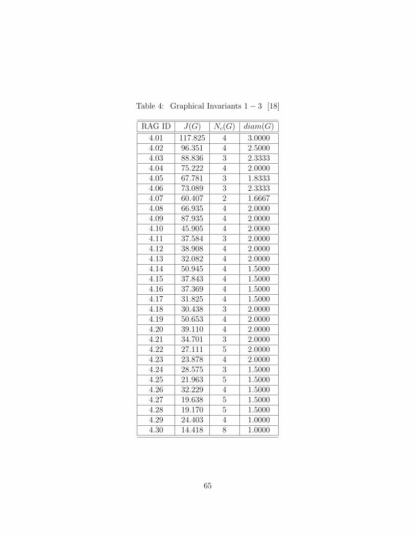
Table 4: Graphical Invariants 1− 3 [18]
RAG ID J(G) Nc(G) diam(G)
4.01 117.825 4 3.00004.02 96.351 4 2.50004.03 88.836 3 2.33334.04 75.222 4 2.00004.05 67.781 3 1.83334.06 73.089 3 2.33334.07 60.407 2 1.66674.08 66.935 4 2.00004.09 87.935 4 2.00004.10 45.905 4 2.00004.11 37.584 3 2.00004.12 38.908 4 2.00004.13 32.082 4 2.00004.14 50.945 4 1.50004.15 37.843 4 1.50004.16 37.369 4 1.50004.17 31.825 4 1.50004.18 30.438 3 2.00004.19 50.653 4 2.00004.20 39.110 4 2.00004.21 34.701 3 2.00004.22 27.111 5 2.00004.23 23.878 4 2.00004.24 28.575 3 1.50004.25 21.963 5 1.50004.26 32.229 4 1.50004.27 19.638 5 1.50004.28 19.170 5 1.50004.29 24.403 4 1.00004.30 14.418 8 1.0000
65
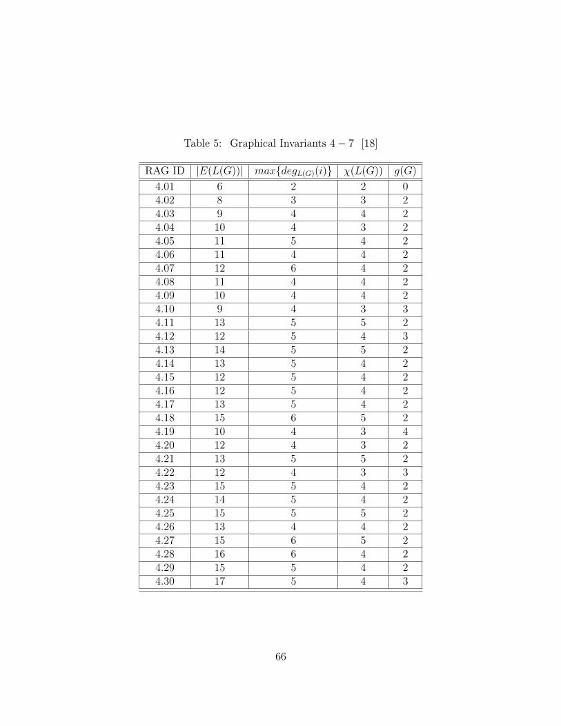
Table 5: Graphical Invariants 4− 7 [18]
RAG ID |E(L(G))| max{degL(G)(i)} χ(L(G)) g(G)
4.01 6 2 2 04.02 8 3 3 24.03 9 4 4 24.04 10 4 3 24.05 11 5 4 24.06 11 4 4 24.07 12 6 4 24.08 11 4 4 24.09 10 4 4 24.10 9 4 3 34.11 13 5 5 24.12 12 5 4 34.13 14 5 5 24.14 13 5 4 24.15 12 5 4 24.16 12 5 4 24.17 13 5 4 24.18 15 6 5 24.19 10 4 3 44.20 12 4 3 24.21 13 5 5 24.22 12 4 3 34.23 15 5 4 24.24 14 5 4 24.25 15 5 5 24.26 13 4 4 24.27 15 6 5 24.28 16 6 4 24.29 15 5 4 24.30 17 5 4 3
66

Table 6: Graphical Invariants 8− 12 [18]
RAG ID W (G) χ′(G) F (G) R(G) γ(G)
4.01 12.0000 3 16 2.8165 2.04.02 10.0000 3 18 2.5749 2.54.03 9.0000 4 20 2.3963 2.54.04 8.0000 3 20 2.3333 2.54.05 7.0000 4 22 2.1547 3.04.06 8.3333 4 22 2.4571 2.04.07 6.0000 4 24 1.9821 3.04.08 7.5000 4 22 2.3963 2.54.09 9.0000 4 20 2.6178 2.04.10 9.5000 4 20 2.5749 1.54.11 7.8333 5 26 2.2356 1.54.12 8.0000 5 24 2.3862 2.04.13 7.0000 5 28 2.2196 2.04.14 5.5000 4 26 2.1178 2.54.15 7.5000 4 24 2.2845 2.04.16 7.5000 4 24 2.2945 2.04.17 6.5000 4 26 2.1547 2.04.18 5.8333 5 30 1.9571 2.04.19 9.5000 3 20 2.4832 2.54.20 7.5000 4 22 2.3333 3.04.21 7.0000 4 26 2.1338 3.04.22 8.0000 3 24 2.3333 2.54.23 7.0000 5 30 2.1178 2.04.24 5.5000 4 28 1.9940 3.54.25 6.5000 4 28 2.1547 1.54.26 6.0000 4 26 2.1547 3.04.27 5.5000 5 34 1.9571 2.04.28 5.5000 4 32 1.9821 2.04.29 4.5000 4 30 1.9880 3.54.30 4.5000 4 34 1.9880 1.5
67
VITA
ALISSA A. ROCKNEY
Education: B.S. Psychology and Mathematics, East Tennessee State
University, Johnson City, Tennessee 2009
M.S. Mathematical Sciences, East Tennessee State
University, Johnson City, TN 2011
Professional Experience: Graduate Teaching Assistant, East Tennessee State
University, Johnson City, Tennessee, 2010-2011
Math Lab Tutor, East Tennessee State University,
Johnson City, Tennessee, 2009-2010
Publications: R. A. Beeler, A. A. Rockney, and C. E. Yearwood, “The
Infinigon and its Properties,”
Congressus Numerantium,
198 (2009) 39–49.
R. A. Beeler and A. A. Rockney, “Decompositions of
Directed Graphs Using Orientations of P4
with a Pendant Edge,”
Congressus Numerantium, 202 (2010) 211–218.
G. C. Blackhart, B. C. Nelson, A. Winter, and A.
Rockney, “Self-control in Relation to Feelings
of Belonging and Acceptance,” Self and Identity,
(2011) 152–165.
68

Awards: Student Travel Award, $400, for the Midsouth Computational
Biology and Bioinformatics Society (MCBIOS), held at
Texas A&M University, April 1-2, 2011
Travel Funding, $300, from the Graduate and Professional Student
Association, East Tennessee State University, for travel
to the Eighth Annual Conference of MCBIOS, held at
Texas A&M University, April 1-2, 2011
Mathematics Award, Department of Mathematics and
Statistics, ETSU, 2009
Faculty Award for the Department of Mathematics and
Statistics, ETSU, 2009
69