Robot Autonomous Perception Model For Internet-Based Intelligent Robotic System

• • • • • • • • • • • • • • • • • • • • • • • • • • • • • • •
A Perception-DrivenAutonomous Urban Vehicle
John Leonard, Jonathan How, Seth Teller,Mitch Berger, Stefan Campbell, Gaston Fiore,Luke Fletcher, Emilio Frazzoli, Albert Huang,Sertac Karaman, Olivier Koch, YoshiakiKuwata, David Moore, Edwin Olson,Steve Peters, Justin Teo, Robert Truax,and Matthew WalterMassachusetts Institute of TechnologyCambridge, Massachusetts 02139e-mail: [email protected]
David Barrett, Alexander Epstein,Keoni Maheloni, and Katy MoyerFranklin W. Olin CollegeNeedham, Massachusetts 02492e-mail: [email protected]
Troy Jones and Ryan BuckleyDraper LaboratoryCambridge, Massachusetts 02139e-mail: [email protected]
Matthew AntoneBAE Systems Advanced InformationTechnologiesBurlington, Massachusetts 01803e-mail: [email protected]
Robert Galejs, Siddhartha Krishnamurthy,and Jonathan WilliamsMIT Lincoln LaboratoryLexington, Massachusetts 02420e-mail: [email protected]
Received 10 February 2008; accepted 22 July 2008
Journal of Field Robotics, 1–48 (2008) C© 2008 Wiley Periodicals, Inc.Published online in Wiley InterScience (www.interscience.wiley.com). • DOI: 10.1002/rob.20262

2 • Journal of Field Robotics—2008
This paper describes the architecture and implementation of an autonomous passengervehicle designed to navigate using locally perceived information in preference to poten-tially inaccurate or incomplete map data. The vehicle architecture was designed to han-dle the original DARPA Urban Challenge requirements of perceiving and navigating aroad network with segments defined by sparse waypoints. The vehicle implementationincludes many heterogeneous sensors with significant communications and computationbandwidth to capture and process high-resolution, high-rate sensor data. The output ofthe comprehensive environmental sensing subsystem is fed into a kinodynamic motionplanning algorithm to generate all vehicle motion. The requirements of driving in lanes,three-point turns, parking, and maneuvering through obstacle fields are all generatedwith a unified planner. A key aspect of the planner is its use of closed-loop simulation ina rapidly exploring randomized trees algorithm, which can randomly explore the spacewhile efficiently generating smooth trajectories in a dynamic and uncertain environment.The overall system was realized through the creation of a powerful new suite of softwaretools for message passing, logging, and visualization. These innovations provide a strongplatform for future research in autonomous driving in global positioning system–deniedand highly dynamic environments with poor a priori information. C© 2008 Wiley Periodicals,
Inc.
1. INTRODUCTION
In November 2007 the Defense Advanced ResearchProjects Agency (DARPA) conducted the DARPAUrban Challenge Event (UCE), which was the thirdin a series of competitions designed to accelerate re-search and development of full-sized autonomousroad vehicles for the defense forces. The competitiveapproach has been very successful in porting a sub-stantial amount of research (and researchers) fromthe mobile robotics and related disciplines into au-tonomous road vehicle research (DARPA, 2007). TheUCE introduced an urban scenario and traffic interac-tions into the competition. The short aim of the com-petition was to develop an autonomous vehicle ca-pable of passing the California driver’s test (DARPA,2007). The 2007 challenge was the first in which auto-mated vehicles were required to obey traffic laws in-cluding lane keeping, intersection precedence, pass-ing, merging, and maneuvering with other traffic.
The contest was held on a closed course withinthe decommissioned George Air Force Base. Thecourse was predominantly the street network of theresidential zone of the former Air Force Base withseveral graded dirt roads added for the contest. Al-though all autonomous vehicles were on the course atthe same time, giving the competition the appearanceof a conventional race, each vehicle was assigned in-dividual missions. These missions were designed byDARPA to require each team to complete 60 mileswithin 6 h to finish the race. In this race againsttime, penalties for erroneous or dangerous behavior
were converted into time penalties. DARPA providedall teams with a single route network definition file(RNDF) 24 h before the race. The RNDF was very sim-ilar to a digital street map used by an in-car globalpositioning system (GPS) navigation system. The filedefined the road positions, number of lanes, inter-sections, and even parking space locations in GPScoordinates. On the day of the race each team wasprovided with a second unique file called a missiondefinition file (MDF). This file consisted solely of alist of checkpoints (or locations) within the RNDFthat the vehicle was required to cross. Each vehiclecompeting in the UCE was required to complete threemissions, defined by three separate MDFs.
Team MIT developed an urban vehicle architec-ture for the UCE. The vehicle (shown in action inFigure 1) was designed to use locally perceived in-formation in preference to potentially inaccurate mapdata to navigate a road network while obeying theroad rules. Three of the key novel features of our sys-tem are (1) a perception-based navigation strategy,(2) a unified planning and control architecture, and(3) a powerful new software infrastructure. Our sys-tem was designed to handle the original race descrip-tion of perceiving and navigating a road networkwith a sparse description, enabling us to completeNational Qualifying Event (NQE) Area B withoutaugmenting the RNDF. Our vehicle utilized a power-ful and general-purpose rapidly exploring random-ized trees (RRT)–based planning algorithm, achiev-ing the requirements of driving in lanes, executingthree-point turns, parking, and maneuvering through
Journal of Field Robotics DOI 10.1002/rob

Leonard et al.: A Perception-Driven Autonomous Urban Vehicle • 3
Figure 1. Talos in action at the NQE.
obstacle fields with a single, unified approach. Thesystem was realized through the creation of a pow-erful new suite of software tools for autonomous ve-hicle research, which our team has made available tothe research community. These innovations providea strong platform for future research in autonomousdriving in GPS-denied and highly dynamic environ-ments with poor a priori information. Team MITwas one of 35 teams that participated in the DARPAUrban Challenge NQE and was one of 11 teams toqualify for the UCE based on our performance in theNQE. The vehicle was one of six to complete the race,finishing in fourth place.
This paper reviews the design and performanceof Talos, the MIT autonomous vehicle. Section 2 sum-marizes the system architecture. Section 3 describesthe design of the race vehicle and software infra-structure. Sections 4 and 5 explain the set of keyalgorithms developed for environmental perceptionand motion planning for the Challenge. Section 6 de-scribes the performance of the integrated system inthe qualifier and race events. Section 7 reflects on howthe perception-driven approach fared by highlight-ing some successes and lessons learned. Section 8provides details on the public release of our team’sdata logs, interprocess communications and imageacquisition libraries, and visualization software.Finally, Section 9 concludes the paper.
2. ARCHITECTURE
Our overall system architecture (Figure 2) includesthe following subsystems:
• The road paint detector uses two differentimage-processing techniques to fit splines tolane markings from the camera data.
• The lane tracker reconciles digital map(RNDF) data with lanes detected by visionand LIDAR to localize the vehicle in the roadnetwork.
• The obstacle detector uses SICK and Velo-dyne LIDAR to identify stationary and mov-ing obstacles.
• The low-lying hazard detector usesdownward-looking LIDAR data to assessthe drivability of the road ahead and to detectcurb cuts.
• The fast vehicle detector uses millimeterwave radar to detect fast-approaching vehi-cles in the medium to long range.
• The positioning module estimates the vehi-cle position in two reference frames. The localframe is an integration of odometry and iner-tial measurement unit (IMU) measurementsto estimate the vehicle’s egomotion throughthe local environment. The global coordinatetransformation estimates the correspondencebetween the local frame and the GPS coordi-nate frame. GPS outages and odometry driftwill vary this transformation. Almost everymodule listens to the positioning module foregomotion correction or path planning.
• The navigator tracks the mission state anddevelops a high-level plan to accomplish themission based on the RNDF and MDF. Theoutput of the robust minimum-time optimiza-tion is a short-term goal location provided tothe motion planner. As progress is made theshort-term goal is moved, like a carrot in frontof a donkey, to achieve the mission.
• The drivability map provides an efficient in-terface to perceptual data, answering queriesfrom the motion planner about the validity ofpotential motion paths. The drivability mapis constructed using perceptual data filteredby the current constraints specified by thenavigator.
• The motion planner identifies, then opti-mizes, a kinodynamically feasible vehicle tra-jectory that moves toward the goal point se-lected by the navigator using the constraintsgiven by the situational awareness embeddedin the drivability map. Uncertainty in local sit-uational awareness is handled through rapid
Journal of Field Robotics DOI 10.1002/rob

4 • Journal of Field Robotics—2008
Figure 2. System architecture.
replanning and constraint tightening. Themotion planner also explicitly accounts forvehicle safety, even with moving obstacles.The output is a desired vehicle trajectory,specified as an ordered list of waypoints (po-sition, velocity, headings) that are provided tothe low-level motion controller.
• The controller executes the low-level motioncontrol necessary to track the desired pathsand velocity profiles issued by the motionplanner.
These modules are supported by a powerful and flex-ible software architecture based on a new lightweightUDP Ethernet protocol message-passing system (de-scribed in Section 3.3). This new architecture facil-itates efficient communication between a suite ofasynchronous software modules operating on the ve-hicle’s distributed computer system. The system hasenabled the rapid creation of a substantial code base,currently approximately 140,000 source lines of code,that incorporates sophisticated capabilities, such asdata logging, replay, and three-dimensional (3-D) vi-sualization of experimental data.
3. INFRASTRUCTURE DESIGN
Achieving an autonomous urban driving capabilityis a difficult multidimensional problem. A key ele-
ment of the difficulty is that significant uncertainty oc-curs at multiple levels: in the environment, in sensing,and in actuation. Any successful strategy for meet-ing this challenge must address all of these sourcesof uncertainty. Moreover, it must do so in a waythat is scalable to spatially extended environmentsand efficient enough for real-time implementation ona rapidly moving vehicle.
The difficulty in developing a solution that canrise to these intellectual challenges is compoundedby the many unknowns in the system design pro-cess. Despite DARPA’s best efforts to define the rulesfor the UCE in detail well in advance of the race,there was huge potential variation in the difficultyof the final event. It was difficult at the start of theproject to conduct a single analysis of the system thatcould be translated to one static set of system require-ments (for example, to predict how different sensorsuites would perform in actual race conditions). Forthis reason, Team MIT chose to follow a spiral designstrategy, developing a flexible vehicle design and cre-ating a system architecture that could respond to anevolution of the system requirements over time, withfrequent testing and incremental addition of newcapabilities as they become available.
Testing “early and often” was a strong recom-mendation of successful participants in the 2005Grand Challenge (Thrun et al., 2006; Trepagnier,Nagel, Kinney, Koutsourgeras, & Dooner, 2006;
Journal of Field Robotics DOI 10.1002/rob

Leonard et al.: A Perception-Driven Autonomous Urban Vehicle • 5
Urmson et al., 2006). As newcomers to the GrandChallenge, it was imperative for our team to obtainan autonomous vehicle as quickly as possible. Hence,we chose to build a prototype vehicle very early in theprogram, while concurrently undertaking the moredetailed design of our final race vehicle. As we gainedexperience from continuous testing with the proto-type, the lessons learned were incorporated into theoverall architecture and our final race vehicle.
The spiral design strategy has manifested itselfin many ways—most dramatically in our decisionto build two (different) autonomous vehicles. We ac-quired our prototype vehicle, a Ford Escape, at theoutset of the project, to permit early autonomous test-ing with a minimal sensor suite. Over time we in-creased the frequency of tests, added sensors, andbrought more software capabilities online to meeta larger set of requirements. In parallel with this,we procured and fabricated our race vehicle Talos, aLand Rover LR3. Our modular and flexible softwarearchitecture was designed to enable a rapid transitionfrom one vehicle to the other. Once the final race ve-hicle became available, all work on the prototype ve-hicle was discontinued, as we followed the adage to“build one system to throw it away.”
3.1. Design Considerations
We employed several key principles in designing oursystem.
Use of many sensors. We chose to use a largenumber of low-cost, unactuated sensors, rather thanto rely exclusively on a small number of more ex-pensive, high-performance sensors. This choice pro-duced the following benefits:
• By avoiding any single point of sensor failure,the system is more robust. It can tolerate lossof a small number of sensors through physicaldamage, optical obscuration, or software fail-ure. Eschewing actuation also simplified themechanical, electrical, and software systems.
• Because each of our many sensors can be po-sitioned at an extreme point on the car, moreof the car’s field of view (FOV) can be ob-served. A single sensor, by contrast, wouldhave a more limited FOV due to unavoid-able occlusion by the vehicle itself. Deploy-ing many single sensors also gave us in-creased flexibility as designers. Most pointsin the car’s surroundings are observed by at
least one of each of the three exteroceptivesensor types. Finally, our multisensor strat-egy also permits more effective distribution ofinput/output (I/O) and CPU bandwidthacross multiple processors.
Minimal reliance on GPS. We observed fromour own prior research and other teams’ prior GrandChallenge efforts that GPS cannot be relied uponfor high-accuracy localization at all times. That fact,along with the observation that humans do not needGPS to drive well, led us to develop a navigationand perception strategy that uses GPS only when ab-solutely necessary, i.e., to determine the general di-rection to the next waypoint and to make forwardprogress in the (rare) case when road markings andboundaries are undetectable. One key outcome of thisdesign choice is our “local frame” situational aware-ness, described more fully in Section 4.1.
Fine-grained, high-bandwidth CPU, I/O, andnetwork resources. Given the short time (18 months,from May 2006 to November 2007) available for sys-tem development, our main goal was simply to geta first pass at every required module working, andworking solidly, in time to qualify. Thus we knew atthe outset that we could not afford to invest effortin premature optimization, i.e., performance profil-ing, memory tuning, etc. This led us to the conclu-sion that we should have many CPUs and that weshould lightly load each machine’s CPU and phys-ical memory (say, at half capacity) to avoid non-linear system effects such as process or memorythrashing. A similar consideration led us to use afast network interconnect, to avoid operating regimesin which network contention became nonnegligible.The downside of our choice of many machines wasa high power budget, which required an externalgenerator on the car. This added mechanical andelectrical complexity to the system, but the com-putational flexibility that was gained justified thiseffort.
Asynchronous sensor publish and update; min-imal sensor fusion. Our vehicle has sensors ofsix different types (odometry, inertial, GPS, LIDAR,radar, vision), each type generating data at a differ-ent rate. Our architecture dedicates a software driverto each individual sensor. Each driver performs min-imal processing and then publishes the sensor dataon a shared network. A “drivability map” applicationprogramming interface (API) (described more fullybelow) performs minimal sensor fusion, simply by
Journal of Field Robotics DOI 10.1002/rob
6 • Journal of Field Robotics—2008
(a) (b)
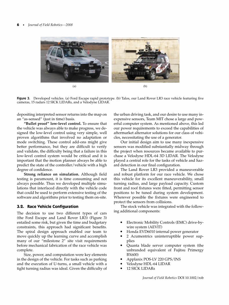
Figure 3. Developed vehicles. (a) Ford Escape rapid prototype. (b) Talos, our Land Rover LR3 race vehicle featuring fivecameras, 15 radars 12 SICK LIDARs, and a Velodyne LIDAR.
depositing interpreted sensor returns into the map onan “as-sensed” (just in time) basis.
“Bullet proof” low-level control. To ensure thatthe vehicle was always able to make progress, we de-signed the low-level control using very simple, wellproven algorithms that involved no adaptation ormode switching. These control add-ons might givebetter performance, but they are difficult to verifyand validate, the difficulty being that a failure in thislow-level control system would be critical and it isimportant that the motion planner always be able topredict the state of the controller/vehicle with a highdegree of confidence.
Strong reliance on simulation. Although fieldtesting is paramount, it is time consuming and notalways possible. Thus we developed multiple simu-lations that interfaced directly with the vehicle codethat could be used to perform extensive testing of thesoftware and algorithms prior to testing them on-site.
3.2. Race Vehicle Configuration
The decision to use two different types of cars(the Ford Escape and Land Rover LR3) (Figure 3)entailed some risk, but given the time and budgetaryconstraints, this approach had significant benefits.The spiral design approach enabled our team tomove quickly up the learning curve and accomplishmany of our “milestone 2” site visit requirementsbefore mechanical fabrication of the race vehicle wascomplete.
Size, power, and computation were key elementsin the design of the vehicle. For tasks such as parkingand the execution of U-turns, a small vehicle with atight turning radius was ideal. Given the difficulty of
the urban driving task, and our desire to use many in-expensive sensors, Team MIT chose a large and pow-erful computer system. As mentioned above, this ledour power requirements to exceed the capabilities ofaftermarket alternator solutions for our class of vehi-cles, necessitating the use of a generator.
Our initial design aim to use many inexpensivesensors was modified substantially midway throughthe project when resources became available to pur-chase a Velodyne HDL-64 3D LIDAR. The Velodyneplayed a central role for the tasks of vehicle and haz-ard detection in our final configuration.
The Land Rover LR3 provided a maneuverableand robust platform for our race vehicle. We chosethis vehicle for its excellent maneuverability, smallturning radius, and large payload capacity. Customfront and roof fixtures were fitted, permitting sensorpositions to be tuned during system development.Wherever possible the fixtures were engineered toprotect the sensors from collisions.
The stock vehicle was integrated with the follow-ing additional components:
• Electronic Mobility Controls (EMC) drive-by-wire system (AEVIT)
• Honda EVD6010 internal power generator• 2 Acumentrics uninterruptible power sup-
plies• Quanta blade server computer system (the
unbranded equivalent of Fujitsu PrimergyBX600)
• Applanix POS-LV 220 GPS/INS• Velodyne HDL-64 LIDAR• 12 SICK LIDARs
Journal of Field Robotics DOI 10.1002/rob

Leonard et al.: A Perception-Driven Autonomous Urban Vehicle • 7
• 5 Point Grey Firefly MV cameras• 15 Delphi radars
The first step in building the LR3 race vehicle wasadapting it for computer-driven control. This taskwas outsourced to EMC in Baton Rouge, Louisiana.They installed computer-controlled servos on thegear shift and steering column and a single servo forthrottle and brake actuation. Their system was de-signed for physically disabled drivers but was adapt-able for our needs. It also provided a proven and safemethod for switching from normal human-drivencontrol to autonomous control.
Safety of the human passengers was a primarydesign consideration in integrating the equipmentinto the LR3. The third row of seats in the LR3 wasremoved, and the entire back end was sectioned offfrom the main passenger cabin by an aluminum andPlexiglas wall. This created a rear “equipment bay,”which held the computer system, the power genera-tor, and all of the power supplies, interconnects, andnetwork hardware for the car. The LR3 was also out-fitted with equipment and generator bay temperaturereadouts, a smoke detector, and a passenger cabincarbon monoxide detector.
The chief consumer of electrical power was theQuanta blade server. The server required 240 V asopposed to the standard 120 V and could consumeup to 4,000 W, dictating many of the power and cool-ing design decisions. Primary power for the systemcame from an internally mounted Honda 6,000-WR/V (recreational vehicle or mobile home) generator.It draws fuel directly from the LR3 tank and produces120 and 240 V ac at 60 Hz. The generator was installedin a sealed aluminum enclosure inside the equipmentbay; cooling air is drawn from outside, and exhaustgases leave through an additional muffler under therear of the LR3.
The 240-V ac power is fed to twin Acumentricsrugged UPS 2500 units that provide backup powerto the computer and sensor systems. The remaininggenerator power is allocated to the equipment bay airconditioning (provided by a roof-mounted R/V airconditioner) and noncritical items such as back-seatpower outlets for passenger laptops.
3.2.1. Sensor Configuration
As mentioned, our architecture is based on the useof many different sensors, based on multiple sensingmodalities. We positioned and oriented the sensors
so that most points in the vehicle’s surroundingswould be observed by at least one sensor of eachtype: LIDAR, radar, and vision. This redundantcoverage gave robustness against both type-specificsensor failure (e.g., difficulty with vision due to lowsun angle) or individual sensor failure (e.g., due towiring damage).
We selected the sensors with several specifictasks in mind. A combination of “skirt” (horizontalSICK) two-dimensional (2-D) LIDARs mountedat a variety of heights, combined with the outputfrom a Velodyne 3-D LIDAR, performs close-rangeobstacle detection. “Pushbroom” (downward-cantedSICK) LIDARs and the Velodyne data detect drivablesurfaces. Out past the LIDAR range, millimeter waveradar detects fast-approaching vehicles. High-rateforward video, with an additional rear video channelfor higher-confidence lane detection, performs lanedetection.
Ethernet interfaces were used to deliver sen-sor data to the computers for most devices. Whenpossible, sensors were connected as Ethernet de-vices. In contrast to many commonly used standardssuch as RS-232, RS-422, serial, controller area net-work (CAN), universal serial bus (USB), or Firewire,Ethernet offers, in one standard, electrical isolation,radio frequency (RF) noise immunity, reasonablephysical connector quality, variable data rates, datamultiplexing, scalability, low latencies, and large datavolumes.
The principal sensor for obstacle detection is theVelodyne HDL-64, which was mounted on a raisedplatform on the roof. High sensor placement was nec-essary to raise the FOV above the SICK LIDAR unitsand the air conditioner. The Velodyne is a 3-D laserscanner composed of 64 lasers mounted on a spin-ning head. It produces approximately a million rangesamples per second, performing a full 360-deg sweepat 15 Hz.
The SICK LIDAR units (all model LMS 291-S05)served as the near-field detection system for obstaclesand the road surface. On the roof rack there are fiveunits angled down viewing the ground ahead of thevehicle, and the remaining seven are mounted loweraround the sides of the vehicle and project outwardparallel to the ground plane.
Each SICK sensor generates an interlaced scanof 180 planar points at a rate of 75 Hz. Each of theSICK LIDAR units has a serial data connection whichis read by a MOXA NPort-6650 serial device server.This unit, mounted in the equipment rack above the
Journal of Field Robotics DOI 10.1002/rob

8 • Journal of Field Robotics—2008
computers, takes up to 16 serial data inputs and out-puts TCP/IP link.
The Applanix POS-LV navigation solution wasused to for world-relative position and orientation es-timation of the vehicle. The Applanix system com-bines differential GPS, a 1-deg of drift per hourrated IMU, and a wheel encoder to estimate thevehicle’s position, orientation, velocity, and rotationrates. The position information was used to deter-mine the relative position of RNDF GPS waypointsto the vehicle. The orientation and rate informa-tion were used to estimate the vehicle’s local motionover time. The Applanix device is interfaced via aTCP/IP link.
Delphi’s millimeter wave OEM automotiveadaptive cruise control radars were used for long-range vehicle tracking. The narrow FOV of theseradars (around 18 deg) required a tiling of 15 radarsto achieve the desired 240-deg FOV. The radars re-quire a dedicated CAN bus interface each. To support15 CAN bus networks, we used eight internally de-veloped CAN to Ethernet adaptors (EthCANs). Eachadaptor could support two CAN buses.
Five Point Grey Firefly MV color cameras wereused on the vehicle, providing close to a 360-deg FOV.Each camera was operated at 22.8 Hz and producedBayer-tiled images at a resolution of 752 × 480. Thisamounted to 39 MB/s of image data, or 2.4 GB/min.To support multiple parallel image processing algo-rithms, camera data were JPEG-compressed and thenretransmitted over UDP multicast to other comput-ers (see Section 3.3.1). This allowed multiple imageprocessing and logging algorithms to operate on thecamera data in parallel with minimal latency.
The primary purpose of the cameras was to de-tect road paint, which was then used to estimate andtrack lanes of travel. Although it is not immediatelyobvious that rearward-facing cameras are useful forthis goal, the low curvature of typical urban roadsmeans that observing lanes behind the vehicle greatlyimproves forward estimates.
The vehicle state was monitored by listening tothe vehicle CAN bus. Wheel speeds, engine rpm,steering wheel position, and gear selection were mon-itored using an EthCAN.
3.2.2. Autonomous Driving Unit
The final link between the computers and the vehi-cle was the autonomous driving unit (ADU). In prin-ciple, it was an interface to the drive-by-wire sys-
tem that we purchased from EMC. In practice, it alsoserved a critical safety role.
The ADU was a very simple piece of hardwarerunning a real-time operating system, executing thecontrol commands passed to it by the non-real-timecomputer cluster. The ADU incorporated a watchdogtimer that would cause the vehicle to automaticallyenter PAUSE state if the computer either generatedinvalid commands or stopped sending commandsentirely.
The ADU also implemented the interface to thebuttons and displays in the cabin, and the DARPA-provided E-stop system. The various states of thevehicle (PAUSE, RUN, STANDBY, E-STOP) weremanaged in a state-machine within the ADU.
3.3. Software Infrastructure
We developed a powerful and flexible software ar-chitecture based on a new lightweight UDP message-passing system. Our system facilitates efficient com-munication between a suite of asynchronous soft-ware modules operating on the vehicle’s distributedcomputer system. This architecture has enabled therapid creation of a substantial code base that incor-porates data logging, replay, and 3-D visualization ofall experimental data, coupled with a powerful simu-lation environment.
3.3.1. Lightweight Communications and Marshalling
Given our emphasis on perception, existing in-terprocess communications infrastructures such asCARMEN (Thrun et al., 2006) or MOOS (Newman,2003) were not sufficient for our needs. We re-quired a low-latency, high-throughput communica-tions framework that scales to many senders andreceivers. After our initial assessment of existing tech-nologies, we designed and implemented an interpro-cess communications system that we call lightweightcommunications and marshaling (LCM).
LCM is a minimalist system for message pass-ing and data marshaling, targeted at real-time sys-tems in which latency is critical. It provides a pub-lish/subscribe message-passing model and an XDR-style message specification language with bindingsfor applications in C, Java, and Python. Messages arepassed via UDP multicast on a switched local areanetwork. Using UDP multicast has the benefit that itis highly scalable; transmitting a message to a thou-sand subscribers uses no more network bandwidththan does transmitting it to one subscriber.
Journal of Field Robotics DOI 10.1002/rob

Leonard et al.: A Perception-Driven Autonomous Urban Vehicle • 9
We maintained two physically separate networksfor different types of traffic. The majority of oursoftware modules communicated via LCM on ourprimary network, which sustained approximately8 MB/s of data throughout the final race. The sec-ondary network carried our full-resolution cameradata and sustained approximately 20 MB/s of datathroughout the final race.
Whereas there certainly was some risk in creatingan entirely new interprocess communications infra-structure, the decision was consistent with our team’soverall philosophy to treat the DARPA Urban Chal-lenge first and foremost as a research project. The de-cision to develop LCM helped to create a strong senseof ownership among the key software developers onthe team. The investment in time required to write,test, and verify the correct operation of the LCM sys-tem paid for itself many times over, by enabling amuch faster development cycle than could have beenachieved with existing interprocess communicationsystems. LCM is now freely available as a tool forwidespread use by the robotics community.
The design of LCM makes it very easy to createlogfiles of all messages transmitted during a specificwindow of time. The logging application simply sub-scribes to every available message channel. As mes-sages are received, they are time-stamped and writ-ten to disk.
To support rapid data analysis and algorithmicdevelopment, we developed a log playback tool thatreads a logfile and retransmits the messages in thelogfile back over the network. Data can be playedback at various speeds, for skimming or careful anal-ysis. Our development cycle frequently involved col-lecting extended data sets with our vehicle and thenreturning to our offices to analyze data and developalgorithms. To streamline the process of analyzinglogfiles, we implemented a user interface in our logplayback tool that supported a number of features,such as randomly seeking to user-specified points inthe logfile, selecting sections of the logfile to repeat-edly play back, extracting portions of a logfile to aseparate smaller logfile, and the selected play back ofmessage channels.
3.3.2. Visualization
The importance of visualizing sensory data as wellas the intermediate and final stages of computationfor any algorithm cannot be overstated. Although ahuman observer does not always know exactly what
to expect from sensors or our algorithms, it is ofteneasy for a human observer to spot when somethingis wrong. We adopted a mantra of “visualize every-thing” and developed a visualization tool called theviewer. Virtually every software module transmitteddata that could be visualized in our viewer, from GPSpose and wheel angles to candidate motion plans andtracked vehicles. The viewer quickly became our pri-mary means of interpreting and understanding thestate of the vehicle and the software systems.
Debugging a system is much easier if data canbe readily visualized. The LCGL library was a simpleset of routines that allowed any section of code in anyprocess on any machine to include in-place OpenGLoperations; instead of being rendered, these opera-tions were recorded and sent across the LCM network(hence LCGL), where they could be rendered by theviewer.
LCGL reduced the amount of effort to create a vi-sualization to nearly zero, with the consequence thatnearly all of our modules have useful debugging vi-sualizations that can be toggled on and off from theviewer.
3.3.3. Process Manager and Mission Manager
The distributed nature of our computing architecturenecessitated the design and implementation of a pro-cess management system, which we called procman.This provided basic failure recovery mechanismssuch as restarting failed or crashed processes, restart-ing processes that have consumed too much systemmemory, and monitoring the processor load on eachof our servers.
To accomplish this task, each server ran an in-stance of a procman deputy, and the operating con-sole ran the only instance of a procman sheriff. As theirnames suggest, the user issues process managementcommands via the sheriff, which then relays com-mands to the deputies. Each deputy is then respon-sible for managing the processes on its server inde-pendent of the sheriff and other deputies. Thus, if thesheriff dies or otherwise loses communication withits deputies, the deputies continue enforcing their lastreceived orders.
Messages passed between sheriffs and deputiesare stateless, and thus it is possible to restart the sher-iff or migrate it across servers without interruptingthe deputies.
The mission manager interface provided a min-imalist user interface for loading, launching, and
Journal of Field Robotics DOI 10.1002/rob

10 • Journal of Field Robotics—2008
aborting missions. This user interface was designedto minimize the potential for human error during thehigh-stress scenarios typical on qualifying runs andrace day. It did so by running various “sanity checks”on the human-specified input, displaying only infor-mation of mission-level relevance and providing aminimal set of intuitive and obvious controls. Us-ing this interface, we routinely averaged well un-der 1 min from the time we received the MDF fromDARPA officials to having our vehicle in pause modeand ready to run.
4. PERCEPTION ALGORITHMS
Team MIT implemented a sensor-rich design for theTalos vehicle. This section describes the algorithmsused to process the sensor data, specifically the lo-cal frame, obstacle detector, hazard detector, and lanetracking modules.
4.1. The Local Frame
The local frame is a smoothly varying coordinateframe into which sensor information is projected. Wedo not rely directly on the GPS position output fromthe Applanix because it is subject to sudden positiondiscontinuities upon entering or leaving areas withpoor GPS coverage. We integrate the velocity esti-mates from the Applanix to get position in the localframe.
The local frame is a Euclidean coordinate systemwith arbitrary origin. It has the desirable propertythat the vehicle always moves smoothly through thiscoordinate system—in other words, it is very accurateover short time scales but may drift relative to itselfover longer time scales. This property makes it idealfor registering the sensor data for the vehicle’s im-mediate environment. An estimate of the coordinatetransformation between the local frame and the GPSreference frame is updated continuously. This trans-formation is needed only when projecting a GPS fea-ture, such as an RNDF waypoint, into the local frame.All other navigation and perceptual reasoning is per-formed directly in the local frame.
A single process is responsible for maintainingand broadcasting the vehicle’s pose in the local frame(position, velocity, acceleration, orientation, and turn-ing rates) as well as the most recent local-to-GPStransformation. These messages are transmitted at100 Hz.
4.2. Obstacle Detector
The system’s large number of sensors provided acomprehensive FOV and provided redundancy bothwithin and across sensor modalities. LIDARs pro-vided near-field obstacle detection (Section 4.2.1),and radars provided awareness of moving vehiclesin the far field (Section 4.2.7).
Much previous work in automotive vehicle track-ing has used computer vision for detecting other carsand other moving objects, such as pedestrians. Ofthe work in the vision literature devoted to track-ing vehicles, the techniques developed by Stein andcollaborators (Stein, Mano, & Shashua, 2000, 2003)are notable because this work provided the basis forthe development of a commercial product: the Mo-bileye automotive visual tracking system. We evalu-ated the Mobileye system; it performed well for track-ing vehicles at front and rear aspects during high-way driving but did not provide a solution that wasgeneral enough for the high-curvature roads, myriadaspect angles, and cluttered situations encounteredin the Urban Challenge. An earlier effort at vision-based obstacle detection (but not velocity estima-tion) employed custom hardware (Bertozzi & Broggi,1998).
A notable detection and tracking system for ur-ban traffic from LIDAR data was developed byWang (2004), who incorporated dynamic object track-ing in a 3-D simultaneous localization and map-ping (SLAM) system. Data association and trackingof moving objects was a prefilter for SLAM pro-cessing, thereby reducing the effects of moving ob-jects in corrupting the map that was being built. Ob-ject tracking algorithms used the interacting multiplemodel (IMM) (Blom & Bar-Shalom, 1988) for proba-bilistic data association. A related project addressedthe tracking of pedestrians and other moving objectsto develop a collision warning system for city busdrivers (Thorpe et al., 2005).
Each UCE team required a method for detect-ing and tracking other vehicles. The techniques ofthe Stanford Racing Team (Stanford Racing Team,2007) and the Tartan Racing Team (Tartan Racing,2007) provide alternative examples of successful ap-proaches. Tartan Racing’s vehicle tracker built on thealgorithm of Mertz et al. (2005), which fits lines toLIDAR returns and estimates convex corners fromthe laser data to detect vehicles. The Stanford team’sobject tracker has similarities to the Team MIT ap-proach. It is based first on filtering out vertical
Journal of Field Robotics DOI 10.1002/rob

Leonard et al.: A Perception-Driven Autonomous Urban Vehicle • 11
(a) (b)
Figure 4. Sensor FOVs (20-m grid size). (a) Our vehicle used seven horizontally mounted 180-deg planar LIDARs withoverlapping FOVs. The three LIDARs at the front and the four LIDARs at the back are drawn separately so that theoverlap can be more easily seen. The ground plane and false positives are rejected using consensus between LIDARs.(b) Fifteen 18-deg radars yield a wide FOV.
obstacles and ground plane measurements, as well asreturns from areas outside of the RNDF. The remain-ing returns are fitted to 2-D rectangles using particlefilters, and velocities are estimated for moving objects(Stanford Racing Team, 2007). Unique aspects of ourapproach are the concurrent processing of LIDARand radar data and a novel multisensor calibrationtechnique.
Our obstacle detection system combines datafrom 7 planar LIDARs oriented in a horizontal con-figuration, a roof-mounted 3-D LIDAR unit, and 15automotive radars. The planar LIDARs were SICKunits returning 180 points at 1-deg spacing, withscans produced at 75 Hz. We used SICK’s “inter-laced” mode, in which every scan is offset 0.25 degfrom the previous scan; this increased the sensitiv-ity of the system to small obstacles. For its largerFOV and longer range, we used the Velodyne “high-definition” LIDAR, which contains 64 lasers arrangedvertically. The whole unit spins, yielding a 360-degscan at 15 Hz.
Our Delphi ACC3 radar units are unique amongour sensors in that they are already deployedon mass-market automobiles to support so-called“adaptive cruise control” at highway speeds. Becauseeach radar has a narrow 18-deg FOV, we arranged 15of them in an overlapping, tiled configuration in or-der to achieve a 256-deg FOV.
The planar LIDAR and radar FOVs are shownin Figure 4. The 360-deg FOV of the Velodyne is aring around the vehicle stretching from 5 to 60 m. A
wide FOV may be achieved either through the useof many sensors (as we did) or by physically actu-ating a smaller number of sensors. Actuated sensorsadd complexity (namely, the actuators, their controlcircuitry, and their feedback sensors), create an addi-tional control problem (which way should the sensorsbe pointed?), and ultimately produce fewer data fora given expenditure of engineering effort. For thesereasons, we chose to use many fixed sensors ratherthan fewer mechanically actuated sensors.
The obstacle tracking system was decoupledinto two largely independent subsystems: one usingLIDAR data, the other using radar. Each subsystemwas tuned individually for a low false-positive rate;the output of the high-level system was the unionof the subsystems’ output. Our simple data fusionscheme allowed each subsystem to be developed ina decoupled and parallel fashion and made it easy toadd or remove a subsystem with a predictable per-formance impact. From a reliability perspective, thisstrategy could prevent a fault in one subsystem fromaffecting another.
4.2.1. LIDAR-Based Obstacle Detection
Our LIDAR obstacle tracking system combined datafrom 12 planar LIDARs (Figure 5) and the VelodyneLIDAR. The Velodyne point cloud was dramati-cally more dense than all of the planar LIDAR datacombined (Figure 6), but including planar LIDARsbrought three significant advantages. First, it was
Journal of Field Robotics DOI 10.1002/rob
12 • Journal of Field Robotics—2008
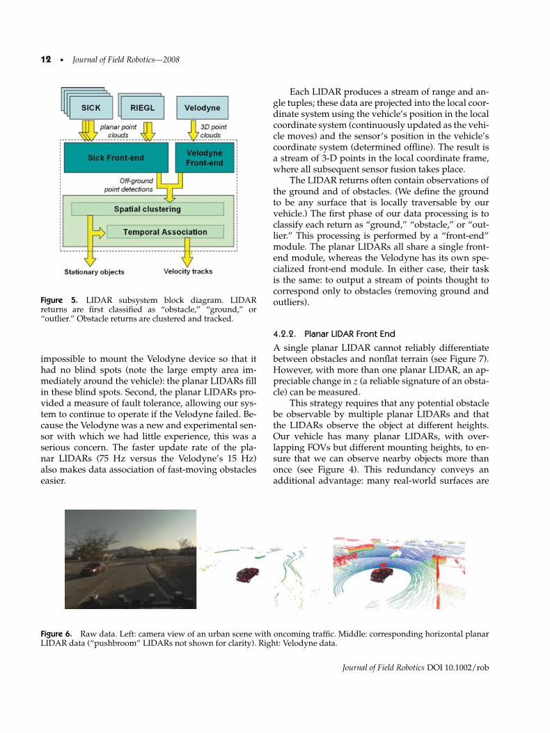
Figure 5. LIDAR subsystem block diagram. LIDARreturns are first classified as “obstacle,” “ground,” or“outlier.” Obstacle returns are clustered and tracked.
impossible to mount the Velodyne device so that ithad no blind spots (note the large empty area im-mediately around the vehicle): the planar LIDARs fillin these blind spots. Second, the planar LIDARs pro-vided a measure of fault tolerance, allowing our sys-tem to continue to operate if the Velodyne failed. Be-cause the Velodyne was a new and experimental sen-sor with which we had little experience, this was aserious concern. The faster update rate of the pla-nar LIDARs (75 Hz versus the Velodyne’s 15 Hz)also makes data association of fast-moving obstacleseasier.
Each LIDAR produces a stream of range and an-gle tuples; these data are projected into the local coor-dinate system using the vehicle’s position in the localcoordinate system (continuously updated as the vehi-cle moves) and the sensor’s position in the vehicle’scoordinate system (determined offline). The result isa stream of 3-D points in the local coordinate frame,where all subsequent sensor fusion takes place.
The LIDAR returns often contain observations ofthe ground and of obstacles. (We define the groundto be any surface that is locally traversable by ourvehicle.) The first phase of our data processing is toclassify each return as “ground,” “obstacle,” or “out-lier.” This processing is performed by a “front-end”module. The planar LIDARs all share a single front-end module, whereas the Velodyne has its own spe-cialized front-end module. In either case, their taskis the same: to output a stream of points thought tocorrespond only to obstacles (removing ground andoutliers).
4.2.2. Planar LIDAR Front End
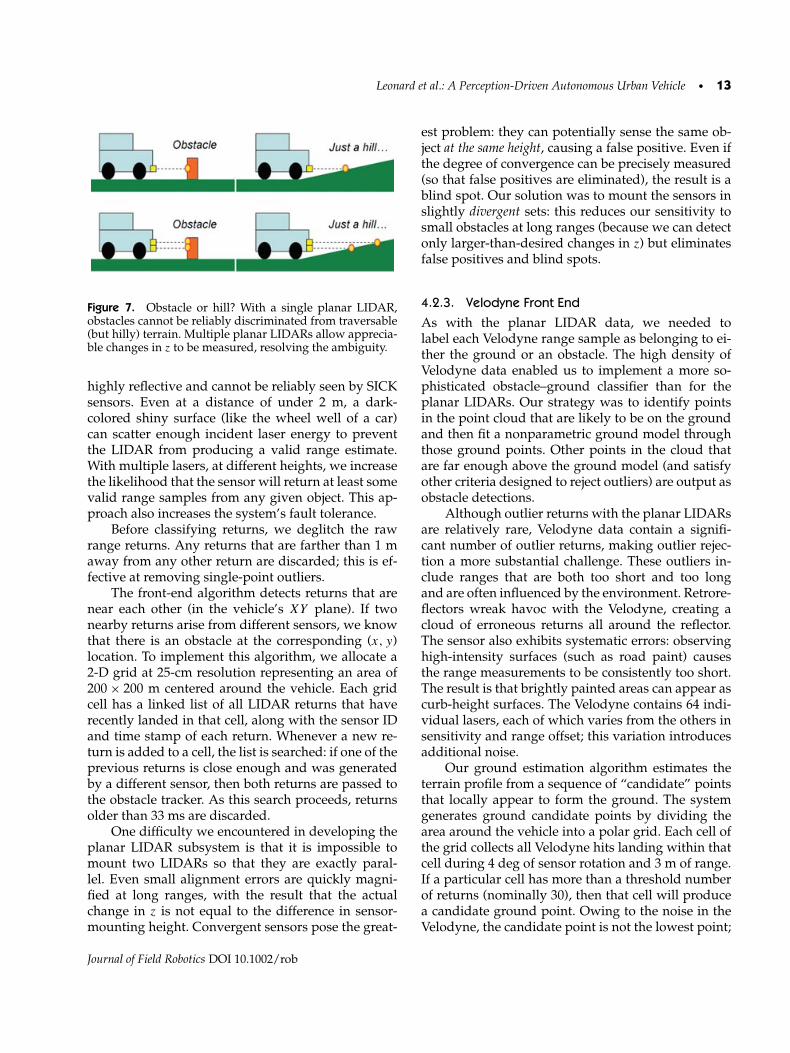
A single planar LIDAR cannot reliably differentiatebetween obstacles and nonflat terrain (see Figure 7).However, with more than one planar LIDAR, an ap-preciable change in z (a reliable signature of an obsta-cle) can be measured.
This strategy requires that any potential obstaclebe observable by multiple planar LIDARs and thatthe LIDARs observe the object at different heights.Our vehicle has many planar LIDARs, with over-lapping FOVs but different mounting heights, to en-sure that we can observe nearby objects more thanonce (see Figure 4). This redundancy conveys anadditional advantage: many real-world surfaces are
Figure 6. Raw data. Left: camera view of an urban scene with oncoming traffic. Middle: corresponding horizontal planarLIDAR data (“pushbroom” LIDARs not shown for clarity). Right: Velodyne data.
Journal of Field Robotics DOI 10.1002/rob
Leonard et al.: A Perception-Driven Autonomous Urban Vehicle • 13
Figure 7. Obstacle or hill? With a single planar LIDAR,obstacles cannot be reliably discriminated from traversable(but hilly) terrain. Multiple planar LIDARs allow apprecia-ble changes in z to be measured, resolving the ambiguity.
highly reflective and cannot be reliably seen by SICKsensors. Even at a distance of under 2 m, a dark-colored shiny surface (like the wheel well of a car)can scatter enough incident laser energy to preventthe LIDAR from producing a valid range estimate.With multiple lasers, at different heights, we increasethe likelihood that the sensor will return at least somevalid range samples from any given object. This ap-proach also increases the system’s fault tolerance.
Before classifying returns, we deglitch the rawrange returns. Any returns that are farther than 1 maway from any other return are discarded; this is ef-fective at removing single-point outliers.
The front-end algorithm detects returns that arenear each other (in the vehicle’s XY plane). If twonearby returns arise from different sensors, we knowthat there is an obstacle at the corresponding (x, y)location. To implement this algorithm, we allocate a2-D grid at 25-cm resolution representing an area of200 × 200 m centered around the vehicle. Each gridcell has a linked list of all LIDAR returns that haverecently landed in that cell, along with the sensor IDand time stamp of each return. Whenever a new re-turn is added to a cell, the list is searched: if one of theprevious returns is close enough and was generatedby a different sensor, then both returns are passed tothe obstacle tracker. As this search proceeds, returnsolder than 33 ms are discarded.
One difficulty we encountered in developing theplanar LIDAR subsystem is that it is impossible tomount two LIDARs so that they are exactly paral-lel. Even small alignment errors are quickly magni-fied at long ranges, with the result that the actualchange in z is not equal to the difference in sensor-mounting height. Convergent sensors pose the great-
est problem: they can potentially sense the same ob-ject at the same height, causing a false positive. Even ifthe degree of convergence can be precisely measured(so that false positives are eliminated), the result is ablind spot. Our solution was to mount the sensors inslightly divergent sets: this reduces our sensitivity tosmall obstacles at long ranges (because we can detectonly larger-than-desired changes in z) but eliminatesfalse positives and blind spots.
4.2.3. Velodyne Front End
As with the planar LIDAR data, we needed tolabel each Velodyne range sample as belonging to ei-ther the ground or an obstacle. The high density ofVelodyne data enabled us to implement a more so-phisticated obstacle–ground classifier than for theplanar LIDARs. Our strategy was to identify pointsin the point cloud that are likely to be on the groundand then fit a nonparametric ground model throughthose ground points. Other points in the cloud thatare far enough above the ground model (and satisfyother criteria designed to reject outliers) are output asobstacle detections.
Although outlier returns with the planar LIDARsare relatively rare, Velodyne data contain a signifi-cant number of outlier returns, making outlier rejec-tion a more substantial challenge. These outliers in-clude ranges that are both too short and too longand are often influenced by the environment. Retrore-flectors wreak havoc with the Velodyne, creating acloud of erroneous returns all around the reflector.The sensor also exhibits systematic errors: observinghigh-intensity surfaces (such as road paint) causesthe range measurements to be consistently too short.The result is that brightly painted areas can appear ascurb-height surfaces. The Velodyne contains 64 indi-vidual lasers, each of which varies from the others insensitivity and range offset; this variation introducesadditional noise.
Our ground estimation algorithm estimates theterrain profile from a sequence of “candidate” pointsthat locally appear to form the ground. The systemgenerates ground candidate points by dividing thearea around the vehicle into a polar grid. Each cell ofthe grid collects all Velodyne hits landing within thatcell during 4 deg of sensor rotation and 3 m of range.If a particular cell has more than a threshold numberof returns (nominally 30), then that cell will producea candidate ground point. Owing to the noise in theVelodyne, the candidate point is not the lowest point;
Journal of Field Robotics DOI 10.1002/rob

14 • Journal of Field Robotics—2008
Figure 8. Ground candidates and interpolation. Velodynereturns are recorded in a polar grid (left: single cell isshown). The lowest 20% (in z height) are rejected as pos-sible outliers; the next lowest return is a ground candidate.A ground model is linearly interpolated through groundcandidates (right), subject to a maximum slope constraint.
instead, the lowest 20% of points (as measured by z)are discarded before the next lowest point is acceptedas a candidate point.
Whereas candidate points often represent thetrue ground, it is possible for elevated surfaces (suchas car roofs) to generate candidates. Thus the systemfilters candidate points further by subjecting themto a maximum ground-slope constraint. We assumethat navigable terrain never exceeds a slope of 0.2(roughly 11 deg). Beginning at our own vehicle’swheels (which, we hope, are on the ground), we pro-cess candidate points in order of increasing distancefrom the vehicle, rejecting those points that would
imply a ground slope in excess of the threshold(Figure 8). The resulting ground model is a polyline(between accepted ground points) for each radial sec-tor (Figure 9).
Explicit ground tracking not only serves as ameans of identifying obstacle points but improvesthe performance of the system over a naive z = 0ground plane model in two complementary ways.First, knowing where the ground is allows the heightof a particular obstacle to be estimated more pre-cisely; this in turn allows the obstacle height thresh-old to be set more aggressively, detecting more actualobstacles with fewer false positives. Second, a groundestimate allows the height above the ground of eachreturn to be computed: obstacles under which the ve-hicle will safely pass (such as overpasses and treecanopies) can thus be rejected.
Given a ground estimate, one could naively clas-sify LIDAR returns as “obstacles” if they are a thresh-old above the ground. However, this strategy is notsufficiently robust to outliers. Individual lasers tendto generate consecutive sequences of outliers: for ro-bustness, it was necessary to require multiple lasersto agree on the presence of an obstacle.
The laser-to-laser calibration noise floor tends tolie just under 15 cm: constantly changing intrinsicvariations across lasers make it impossible to reliablymeasure, across lasers, height changes smaller than
Figure 9. Ground model example. On hilly terrain, the terrain deviates significantly from a plane but is tracked fairly wellby the ground model.
Journal of Field Robotics DOI 10.1002/rob

Leonard et al.: A Perception-Driven Autonomous Urban Vehicle • 15
this. Thus the overlying algorithm cannot reliably de-tect obstacles shorter than about 15 cm.
For each polar cell, we tally the number of returnsgenerated by each laser that is above the ground byan “evidence” threshold (nominally 15 cm). Then,we consider each return again: those returns that areabove the ground plane by a slightly larger threshold(25 cm) and are supported by enough evidence arelabeled as obstacles. The evidence criteria can be sat-isfied in two ways: by three lasers each with at leastthree returns or by five lasers with one hit. This mixincreases sensitivity over any single criterion whilestill providing robustness to erroneous data from anysingle laser.
The difference between the “evidence” thresh-old (15 cm) and the “obstacle” threshold (25 cm) isdesigned to increase the sensitivity of the obstacledetector to low-lying obstacles. If we used the evi-dence threshold alone (15 cm), we would have toomany false positives because that threshold is nearthe noise floor. Conversely, using the 25-cm thresholdalone would require obstacles to be significantly tallerthan 25 cm because we must require multiple lasers toagree and each laser has a different pitch angle. Com-bining these two thresholds increases the sensitivitywithout significantly affecting the false-positive rate.
All of the algorithms used on the Velodyne op-erate on a single sector of data rather than waitingfor a whole scan. If whole scans were used, the mo-tion of the vehicle would inevitably create a seam orgap in the scan. Sector-wise processing also reducesthe latency of the system: obstacle detections can bepassed to the obstacle tracker every 3 ms (the delaybetween the first and last laser to scan at a particu-lar bearing) rather than every 66 ms (the rotationalperiod of the sensor). During the saved 63 ms, a cartraveling at 15 m/s would travel almost 1 m. Everybit of latency that can be saved increases the safety ofthe system by providing earlier warning of danger.
4.2.4. Clustering
The Velodyne alone produces up to a million hits persecond; tracking individual hits over time is compu-tationally prohibitive and unnecessary. Our first stepwas in data reduction: reducing the large number ofhits to a much smaller number of “chunks.” A chunkis simply a record of multiple, spatially close-rangesamples. The chunks also serve as the mechanism forfusion of planar LIDAR and Velodyne data: obstacle
detections from both front ends are used to create andupdate chunks.
One obvious implementation of chunking couldbe through a grid map, by tallying hits within eachcell. However, such a representation is subject to sig-nificant quantization effects when objects lie near cellboundaries. This is especially problematic when us-ing a coarse spatial resolution.
Instead, we used a representation in which in-dividual chunks of bounded size could be centeredarbitrarily. This permitted us to use a coarse spa-tial decimation (reducing our memory and compu-tational requirements) while avoiding the quantiza-tion effects of a grid-based representation. In addi-tion, we recorded the actual extent of the chunk: thechunks have a maximum size but not a minimum size.This allows us to approximate the shape and extent ofobstacles much more accurately than would a grid-map method. This floating “chunk” representationyields a better approximation of an obstacle’s bound-ary without the costs associated with a fine-resolutiongrid map.
Chunks are indexed using a 2-D lookup tablewith about 1-m resolution. Finding the chunk near-est a point p involves searching through all the gridcells that could contain a chunk that contains p. Butbecause the size of a chunk is bounded, the number ofgrid cells and chunks is also bounded. Consequently,lookups remain an O(1) operation.
For every obstacle detection produced by a frontend, the closest chunk is found by searching the 2-Dlookup table. If the point lies within the closest chunkor the chunk can be enlarged to contain the pointwithout exceeding the maximum chunk dimension(35 cm), the chunk is appropriately enlarged and ourwork is done. Otherwise, a new chunk is created; ini-tially it will contain only the new point and will thushave zero size.
Periodically, every chunk is reexamined. If a newpoint has not been assigned to the chunk within thelast 250 ms, the chunk expires and is removed fromthe system.
A physical object is typically represented by morethan one chunk. To compute the velocity of obsta-cles, we must know which chunks correspond to thesame physical objects. To determine this, we clusteredchunks into groups; any two chunks within 25 cmof one another were grouped as the same physicalobject. This clustering operation is outlined inAlgorithm 1.
Journal of Field Robotics DOI 10.1002/rob

16 • Journal of Field Robotics—2008
Algorithm 1 Chunk Clustering
1: Create a graph G with a vertex for each chunk and noedges2: for all c ∈ chunks do3: for all chunks d within ε of c do4: Add an edge between c and d
5: end for6: end for7: Output connected components of G.
Algorithm 1 requires a relatively small amount ofCPU time. The time required to search within a fixedradius of a particular chunk is in fact O(1), becausethere is a constant bound on the number of chunksthat can simultaneously exist within that radius, andthese chunks can be found in O(1) time by iterat-ing over the 2-D lookup table that stores all chunks.The cost of merging subgraphs, implemented by theUnion-Find algorithm (Rivest & Leiserson, 1990), hasa complexity of less than O(log N ). In aggregate, thetotal complexity is less than O(N log N ).
4.2.5. Tracking
The goal of clustering chunks into groups is to iden-tify connected components so that we can track themover time. The clustering operation described aboveis repeated at a rate of 15 Hz. Note that chunks arepersistent: a given chunk will be assigned to multiplegroups, one at each time step.
At each time step, the new groups are associatedwith a group from the previous time step. This isdone via a voting scheme; the new group that over-laps (in terms of the number of chunks) the most
with an old group is associated with the old group.This algorithm yields a fluid estimate of which ob-jects are connected to each other: it is not necessaryto explicitly handle groups that appear to merge orsplit.
The bounding boxes for two associated groups(separated in time) are compared, yielding a velocityestimate. These instantaneous velocity estimates tendto be noisy: our view of obstacles tends to changeover time due to occlusion and scene geometry,with corresponding changes in the apparent size ofobstacles.
Obstacle velocities are filtered over time in thechunks. Suppose that two sets of chunks are asso-ciated with each other, yielding a velocity estimate.That velocity estimate is then used to update the con-stituent chunks’ velocity estimates. Each chunk’s ve-locity estimate is maintained with a trivial Kalmanfilter, with each observation having equal weight.
Storing velocities in the chunks conveys a signif-icant advantage over maintaining separate “tracks”:if the segmentation of a scene changes, resulting inmore or fewer tracks, the new groups will inherit rea-sonable velocities due to their constituent chunks. Be-cause the segmentation is fairly volatile due to oc-clusion and changing scene geometry, maintainingvelocities in the chunks provides greater continu-ity than would result from frequently creating newtracks.
Finally, we output obstacle detections using thecurrent group segmentation (Figure 10), with eachgroup reported as having a velocity equal to theweighted average of its constituent chunks. (Theweights are simply the confidence of each individualchunk’s velocity estimate.)
Figure 10. LIDAR obstacle detections. Our vehicle is in the center; nearby (irregular) walls are shown, clustered accord-ing to physical proximity to each other. Two other cars are visible as bounding boxes with lines indicating the estimatedvelocities: an oncoming car ahead and to the left and another vehicle following us (a chase car). The long lines with arrowsindicate the nominal travel lanes: they are included to aid interpretation but were not used by the tracker.
Journal of Field Robotics DOI 10.1002/rob

Leonard et al.: A Perception-Driven Autonomous Urban Vehicle • 17
A core strength of our system is its ability to pro-duce velocity estimates for rapidly moving objectswith very low latency. This was a design goal becausefast-moving objects represent the most acute safetyhazard.
The corresponding weakness of our system isin estimating the velocity of slow-moving obstacles.Accurately measuring small velocities requires care-ful tracking of an object over relatively long periodsof time. Our system averages instantaneous velocitymeasurements, but these instantaneous velocitymeasurements are contaminated by noise that caneasily swamp small velocities. In practice, we foundthat the system could reliably track objects movingfaster than 3 m/s. The motion planner avoids “closecalls” with all obstacles, keeping the vehicle awayfrom them. Improving tracking of slow-movingobstacles remains a goal for future work.
Another challenge is the “aperture” problem, inwhich a portion of a static obstacle is sensed througha small gap. The motion of our own vehicle can makeit appear that an obstacle is moving on the other sideof the aperture. Whereas apertures could be detectedand explicitly filtered, the resulting phantom obsta-cles tend to have velocities parallel to our own vehicleand thus do not significantly affect motion planning.
Our system operates without a prior on the loca-tion of the road. Prior information on the road couldbe profitably used to eliminate false positives (by as-suming that moving cars must be on the road, for ex-ample), but we chose not to use a prior for two rea-sons. Critically, we wanted our system to be robust tomoving objects anywhere, including those that mightbe pulling out of a driveway or jaywalking pedestri-ans. Second, we wanted to be able to test our detectorin a wide variety of environments without having tofirst generate the corresponding metadata.
4.2.6. LIDAR Tracking Results
The algorithm performed with high reliability, cor-rectly detecting obstacles including a thin metallicgate that errantly closed across our path.
In addition to filling in blind spots (to theVelodyne) immediately around the vehicle, the SICKLIDARs reinforced the obstacle tracking perfor-mance. To quantitatively measure the effectiveness ofthe planar LIDARs (as a set) versus the Velodyne, wetabulated the maximum range at which each subsys-tem first observed an obstacle (specifically, a chunk).We consider only chunks that were, at one point in
Figure 11. Detection range by sensor. For each of 40,000chunks, the earliest detection of the chunk was collected foreach modality (Velodyne and SICK). The Velodyne’s per-formance was substantially better than that of the SICK’s,which observed fewer objects.
time, the closest to the vehicle along a particularbearing; the Velodyne senses many obstacles fartheraway, but in general, it is the closest obstacle that ismost important. Statistics gathered over the lifetimesof 40,000 chunks (see Figure 11) indicate the follow-ing:
• The Velodyne tracked 95.6% of all the obsta-cles that appeared in the system; the SICKsalone tracked 61.0% of obstacles.
• The union of the two subsystems yieldeda minor, but measurable, improvement with96.7% of all obstacles tracked.
• Of those objects tracked by both the Velodyneand the SICK, the Velodyne detected the ob-ject at a longer range: 1.2 m on average.
In complex environments, such as the one used inthis data set, the ground is often nonflat. As a result,planar LIDARs often find themselves observing skyor dirt. Whereas we can reject the dirt as an obstacle(due to our use of multiple LIDARs), we cannot seethe obstacles that might exist nearby. The Velodyne,with its large vertical FOV, is largely immune to thisproblem: we attribute the Velodyne subsystem’s su-perior performance to this difference. The Velodynecould also see over and sometimes through other ob-stacles (i.e., foliage), which would allow it to detectobstacles earlier.
One advantage of the SICKs was their higher ro-tational rate (75 Hz versus the Velodyne’s 15 Hz),which makes data association easier for fast-moving
Journal of Field Robotics DOI 10.1002/rob

18 • Journal of Field Robotics—2008
(a) (b)
Figure 12. Radar tracking three vehicles. (a) Front right camera showing three traffic vehicles, one oncoming. (b) Points:Raw radar detections with tails representing the Doppler velocity. Rectangles: Resultant vehicle tracks with speed in metersper second (rectangle size is simply for visualization).
obstacles. If another vehicle is moving at 15 m/s, theVelodyne will observe a 1-m displacement betweenscans, whereas the SICKs will observe only a 0.2-mdisplacement between scans.
4.2.7. Radar-Based Fast-Vehicle Detection
The radar subsystem complements the LIDAR sub-system by detecting moving objects at ranges beyondthe reliable detection range of the LIDARs. In addi-tion to range and bearing, the radars directly mea-sure the closing rate of moving objects using Doppler,greatly simplifying data association. Each radar has aFOV of 18 deg. To achieve a wide FOV, we tiled 15radars (see Figure 4).
The radar subsystem maintains a set of activetracks. We propagate these tracks forward in timewhenever the radar produces new data, so that wecan compare the predicted position and velocity tothe data returned by the radar.
The first step in tracking is to associate radardetections to any active tracks. The radar producesDoppler closing rates that are consistently within afew meters per second of the truth: if the predictedclosing rate and the measured closing rate differ bymore than 2 m/s, we disallow a match. Otherwise,the closest track (in the XY plane) is chosen foreach measurement. If the closest track is more than6.0 m from the radar detection, a new track is createdinstead.
Each track records all radar measurements thathave been matched to it over the last second. We up-date each track’s position and velocity model by com-puting a least-squares fit of a constant-velocity modelto the (x, y, time) data from the radars. We weightrecent observations more strongly than older obser-vations because the target may be accelerating. For
simplicity, we fitted the constant-velocity model us-ing just the (x, y) points; whereas the Doppler datacould probably be profitably used, this simpler ap-proach produced excellent results. Figure 12 showsa typical output from the radar data association andtracking module. Although no lane data were usedin the radar tracking module, the vehicle track direc-tions match well. The module is able to facilitate theoverall objective of detecting when to avoid enteringan intersection due to fast-approaching vehicles.
Unfortunately, the radars cannot easily distin-guish between small, innocuous objects (such as abolt lying on the ground, or a sewer grate) and largeobjects (such as cars). To avoid false positives, weused the radars only to detect moving objects.
4.3. Hazard Detector
We define hazards as objects that we shouldn’t driveover, even if the vehicle probably could. Hazards in-clude potholes, curbs, and other small objects. Thehazard detector is not intended to detect cars andother large (potentially moving) objects: instead, thegoal of the module is to estimate the condition of theroad itself.
In addition to the Velodyne, Talos used fivedownward-canted planar LIDARs positioned on theroof: these were primarily responsible for observingthe road surface. The basic principle of the hazarddetector is to look for z-height discontinuities in thelaser scans. Over a small batch of consecutive laser re-turns, the z slope is computed by dividing the changein z by the distance between the individual returns.This slope is accumulated in a grid map that recordsthe largest slope observed in every cell. This grid mapis slowly built up over time as the sensors pass overnew ground and extended for about 40 m in every
Journal of Field Robotics DOI 10.1002/rob

Leonard et al.: A Perception-Driven Autonomous Urban Vehicle • 19
direction. Data that “fell off” the grid map (by beingmore than 40 m away) were forgotten.
The Velodyne sensor, with its 64 lasers, could ob-serve a large area around the vehicle. However, haz-ards can be detected only where lasers actually strikethe ground: the Velodyne’s lasers strike the ground in64 concentric circles around the vehicle with signifi-cant gaps between the circles. However, these gapsare filled in as the vehicle moves. Before we obtainedthe Velodyne, our system relied on only the five pla-nar SICK LIDARs with even larger gaps between thelasers.
The laser-to-laser calibration of the Velodyne wasnot sufficiently reliable or consistent to allow verti-cal discontinuities to be detected by comparing the z
heights measured by different physical lasers. Con-sequently, we treated each Velodyne laser indepen-dently as a line scanner.
Unlike the obstacle detector, which assumes thatobstacles will be constantly reobserved over time, thehazard detector is significantly more stateful becausethe largest slope ever observed is remembered foreach (x, y) grid cell. This “running maximum” strat-egy was necessary because any particular line scanacross a hazard samples the change in height onlyalong one direction. A vertical discontinuity alongany direction, however, is potentially hazardous. Agood example of this anisotropic sensitivity is a curb:when a line scanner samples parallel to the curb,no discontinuity is detected. Only when the curb isscanned perpendicularly does a hazard result. Wemounted our SICK sensors so that they would likelysample the curb at a roughly perpendicular angle (as-suming that we are driving parallel to the curb), butultimately, a diversity of sampling angles was criticalto reliably sensing hazards.
4.3.1. Removal of Moving Objects
The grid map described above, which records theworst z slope seen at each (x, y) location, would tendto detect moving cars as large hazards smeared acrossthe moving car’s trajectory. This is undesirable be-cause we wish to determine the condition of the roadbeneath the car.
Our solution was to run an additional “smooth”detector in parallel with the hazard detector. Themaximum and minimum z heights occurring during100-ms integration periods are stored in the grid map.Next, 3 × 3 neighborhoods of the grid map are exam-ined: if all nine areas have received a sufficient num-
ber of measurements and the maximum difference inz is small, the grid cell is labeled as “smooth.” Thisclassification overrides any hazard detection. If a cardrives through our FOV, it may result in temporaryhazards, but as soon as the ground beneath the car isvisible, the ground will be marked as smooth instead.
The output of the hazard and smooth detector isshown later in Figure 26(a). The hazard map showslighter regions on the road ahead and behind the ve-hicle indicating smooth terrain. Along the edge ofthe road darker regions reflect uneven terrain suchas curb cuts or berms.
4.3.2. Hazards as High-Cost Regions
The hazard map was incorporated by the drivabilitymap as high-cost regions. Motion plans that passedover hazardous terrain were penalized but not ruledout entirely. This is because the hazard detector wasprone to false positives for two reasons. First, itwas tuned to be highly sensitive so that even shortcurbs would be detected. Second, because the costmap was a function of the worst-ever-seen z slope,a false positive could cause a phantom hazard thatwould last forever. In practice, associating a cost withcurbs and other hazards was sufficient to keep thevehicle from running over them; at the same time,the only consequence of a false positive was that wemight veer around a phantom. A false positive couldnot cause the vehicle to get stuck.
4.3.3. Road-Edge Detector
Hazards often occur at the road edge, and our de-tector readily detects them. Berms, curbs, and tallgrass all produce hazards that are readily differenti-ated from the road surface itself.
We detect the road edge by casting rays fromthe vehicle’s current position and recording the firsthigh-hazard cell in the grid map [see Figure 13(a)].This results in a number of road-edge point detec-tions; these are segmented into chains based on theirphysical proximity to each other. A nonparametriccurve is then fitted through each chain [shown inFigure 13(b)]. Chains that are either very short orhave excessive curvature are discarded; the rest areoutput to other parts of the system.
4.4. Lane Finding
Our approach to lane finding involves three stages.In the first, the system detects and localizes painted
Journal of Field Robotics DOI 10.1002/rob

20 • Journal of Field Robotics—2008
(a) (b)
Figure 13. Hazard map: Light regions on the road indicate smooth terrain. Dark regions along the road edge indicateuneven terrain such as curb cuts or berms. (a) Rays radiating from vehicle used to detect the road edge. (b) Polylines fittedto road edge.
road markings in each video frame, using LIDARdata to reduce the false-positive detection rate. A sec-ond stage processes the road-paint detections alongwith LIDAR-detected curbs (see Section 4.3) to esti-mate the centerlines of nearby travel lanes. Finally,the detected centerlines output by the second stageare filtered, tracked, and fused with a weak prior toproduce one or more nonparametric lane outputs.
4.4.1. Absolute Camera Calibration
Our road-paint detection algorithms assume thatGPS and IMU navigation data are available of suf-ficient quality to correct for short-term variations invehicle heading, pitch, and roll during image process-ing. In addition, the intrinsic (focal length, center, anddistortion) and extrinsic (vehicle-relative pose) pa-rameters of the cameras have been calibrated aheadof time. This “absolute calibration” allows prepro-cessing of the images in several ways (Figure 14):
• The horizon line is projected into each im-age frame. Only pixel rows below this line areconsidered for further processing.
• Our LIDAR-based obstacle detector suppliesreal-time information about the location ofobstructions in the vicinity of the vehicle.These obstacles are projected into the imageand their extent masked out during the paint-detection algorithms, an important step in re-ducing false positives.
• The inertial data allow us to project the ex-pected location of the ground plane into the
image, providing a useful prior for the paint-detection algorithms.
• False paint detections caused by lens flare canbe detected and rejected. Knowing the timeof day and our vehicle pose relative to theEarth, we can compute the ephemeris of thesun. Line estimates that point toward the sunin image coordinates are removed.
4.4.2. Road-Paint Detection
We employ two algorithms for detecting patternsof road paint that constitute lane boundaries. Bothalgorithms accept raw frames as input and producesets of connected line segments, expressed in thelocal coordinate frame, as output. The algorithms are
Figure 14. Use of absolute camera calibration to projectreal-world quantities into the image.
Journal of Field Robotics DOI 10.1002/rob

Leonard et al.: A Perception-Driven Autonomous Urban Vehicle • 21
Figure 15. The matched filter–based detector from start tofinish. The original image is convolved with a matched fil-ter at each row (horizontal filter shown here). Local max-ima in the filter response are enumerated and their domi-nant orientations computed. The figure depicts orientationby drawing the perpendiculars to each maximum. Finally,nearby maxima are connected into cubic hermite splines.
stateless; each frame from each camera is consideredindependently, deferring spatial–temporal boundaryfusion and tracking to higher level downstreamstages.
The first algorithm applies one-dimensional hor-izontal and vertical matched filters (for lines alongand transverse to the line of sight, respectively)whose support corresponds to the expected widthof a painted line marking projected onto each imagerow. As shown in Figure 15, the filters successfullydiscard most scene clutter while producing strongresponses along line-like features. We identify localmaxima of the filter responses and for each maximumcompute the principal line direction as the domi-nant eigenvector of the Hessian in a local windowcentered at that maximum. The algorithm finally con-
Figure 16. Progression from original image throughsmoothed gradients, border contours, and symmetric con-tour pairs to form centerline candidate.
nects nearby maxima into splines that represent con-tinuous line markings; connections are establishedby growing spline candidates from a set of randomseeds, guided by a distance transform function gen-erated from the entire list of maxima.
The second algorithm for road-paint detectionidentifies potential paint boundary pairs that areproximal and roughly parallel in real-world spaceand whose local gradients point toward each other(Figure 16). We compute the direction and mag-nitude of the image’s spatial gradients, which un-dergo thresholding and nonmaximal suppression toproduce a sparse feature mask. Next, a connectedcomponents algorithm walks the mask to generatesmooth contours of ordered points, broken at dis-continuities in location and gradient direction. A sec-ond iterative walk then grows centerline curves be-tween contours with opposite-pointing gradients. Weenforce global smoothness and curvature constraintsby fitting parabolas to the resulting curves and re-cursively breaking them at points of high deviationor spatial gaps. We finally remove all curves shorterthan a given threshold length to produce the finalroad paint-line outputs.
4.4.3. Lane Centerline Estimation
The second stage of lane finding estimates the geom-etry of nearby lanes using a weighted set of recentroad-paint and curb detections, both of which are rep-resented as piecewise linear curves. Lane centerlinesare represented as locally parabolic segments and areestimated in two steps. First, a centerline evidenceimage D is constructed, where the value of each pixel
Journal of Field Robotics DOI 10.1002/rob
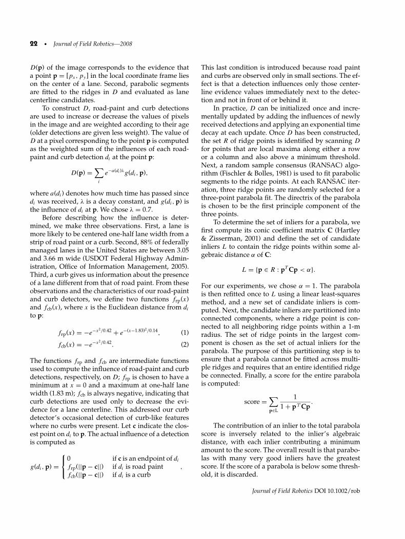
22 • Journal of Field Robotics—2008
D(p) of the image corresponds to the evidence thata point p = [px, py] in the local coordinate frame lieson the center of a lane. Second, parabolic segmentsare fitted to the ridges in D and evaluated as lanecenterline candidates.
To construct D, road-paint and curb detectionsare used to increase or decrease the values of pixelsin the image and are weighted according to their age(older detections are given less weight). The value ofD at a pixel corresponding to the point p is computedas the weighted sum of the influences of each road-paint and curb detection di at the point p:
D(p) =∑
i
e−a(di )λg(di, p),
where a(di) denotes how much time has passed sincedi was received, λ is a decay constant, and g(di, p) isthe influence of di at p. We chose λ = 0.7.
Before describing how the influence is deter-mined, we make three observations. First, a lane ismore likely to be centered one-half lane width from astrip of road paint or a curb. Second, 88% of federallymanaged lanes in the United States are between 3.05and 3.66 m wide (USDOT Federal Highway Admin-istration, Office of Information Management, 2005).Third, a curb gives us information about the presenceof a lane different from that of road paint. From theseobservations and the characteristics of our road-paintand curb detectors, we define two functions frp(x)and fcb(x), where x is the Euclidean distance from di
to p:
frp(x) = −e−x2/0.42 + e−(x−1.83)2/0.14, (1)
fcb(x) = −e−x2/0.42. (2)
The functions frp and fcb are intermediate functionsused to compute the influence of road-paint and curbdetections, respectively, on D; frp is chosen to have aminimum at x = 0 and a maximum at one-half lanewidth (1.83 m); fcb is always negative, indicating thatcurb detections are used only to decrease the evi-dence for a lane centerline. This addressed our curbdetector’s occasional detection of curb-like featureswhere no curbs were present. Let c indicate the clos-est point on di to p. The actual influence of a detectionis computed as
g(di, p) =⎧⎨⎩
0 if c is an endpoint of di
frp(||p − c||) if di is road paintfcb(||p − c||) if di is a curb
,
This last condition is introduced because road paintand curbs are observed only in small sections. The ef-fect is that a detection influences only those center-line evidence values immediately next to the detec-tion and not in front of or behind it.
In practice, D can be initialized once and incre-mentally updated by adding the influences of newlyreceived detections and applying an exponential timedecay at each update. Once D has been constructed,the set R of ridge points is identified by scanning D
for points that are local maxima along either a rowor a column and also above a minimum threshold.Next, a random sample consensus (RANSAC) algo-rithm (Fischler & Bolles, 1981) is used to fit parabolicsegments to the ridge points. At each RANSAC iter-ation, three ridge points are randomly selected for athree-point parabola fit. The directrix of the parabolais chosen to be the first principle component of thethree points.
To determine the set of inliers for a parabola, wefirst compute its conic coefficient matrix C (Hartley& Zisserman, 2001) and define the set of candidateinliers L to contain the ridge points within some al-gebraic distance α of C:
L = {p ∈ R : pT Cp < α}.
For our experiments, we chose α = 1. The parabolais then refitted once to L using a linear least-squaresmethod, and a new set of candidate inliers is com-puted. Next, the candidate inliers are partitioned intoconnected components, where a ridge point is con-nected to all neighboring ridge points within a 1-mradius. The set of ridge points in the largest com-ponent is chosen as the set of actual inliers for theparabola. The purpose of this partitioning step is toensure that a parabola cannot be fitted across multi-ple ridges and requires that an entire identified ridgebe connected. Finally, a score for the entire parabolais computed:
score =∑p∈L
11 + pT Cp
.
The contribution of an inlier to the total parabolascore is inversely related to the inlier’s algebraicdistance, with each inlier contributing a minimumamount to the score. The overall result is that parabo-las with many very good inliers have the greatestscore. If the score of a parabola is below some thresh-old, it is discarded.
Journal of Field Robotics DOI 10.1002/rob
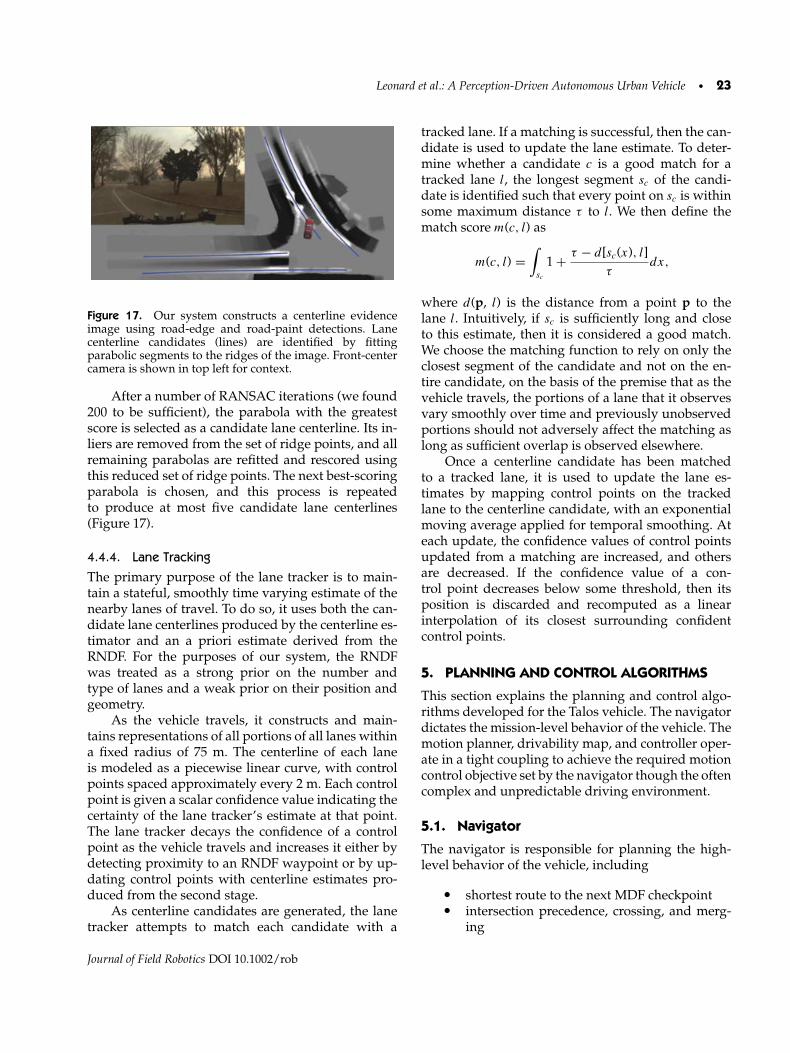
Leonard et al.: A Perception-Driven Autonomous Urban Vehicle • 23
Figure 17. Our system constructs a centerline evidenceimage using road-edge and road-paint detections. Lanecenterline candidates (lines) are identified by fittingparabolic segments to the ridges of the image. Front-centercamera is shown in top left for context.
After a number of RANSAC iterations (we found200 to be sufficient), the parabola with the greatestscore is selected as a candidate lane centerline. Its in-liers are removed from the set of ridge points, and allremaining parabolas are refitted and rescored usingthis reduced set of ridge points. The next best-scoringparabola is chosen, and this process is repeatedto produce at most five candidate lane centerlines(Figure 17).
4.4.4. Lane Tracking
The primary purpose of the lane tracker is to main-tain a stateful, smoothly time varying estimate of thenearby lanes of travel. To do so, it uses both the can-didate lane centerlines produced by the centerline es-timator and an a priori estimate derived from theRNDF. For the purposes of our system, the RNDFwas treated as a strong prior on the number andtype of lanes and a weak prior on their position andgeometry.
As the vehicle travels, it constructs and main-tains representations of all portions of all lanes withina fixed radius of 75 m. The centerline of each laneis modeled as a piecewise linear curve, with controlpoints spaced approximately every 2 m. Each controlpoint is given a scalar confidence value indicating thecertainty of the lane tracker’s estimate at that point.The lane tracker decays the confidence of a controlpoint as the vehicle travels and increases it either bydetecting proximity to an RNDF waypoint or by up-dating control points with centerline estimates pro-duced from the second stage.
As centerline candidates are generated, the lanetracker attempts to match each candidate with a
tracked lane. If a matching is successful, then the can-didate is used to update the lane estimate. To deter-mine whether a candidate c is a good match for atracked lane l, the longest segment sc of the candi-date is identified such that every point on sc is withinsome maximum distance τ to l. We then define thematch score m(c, l) as
m(c, l) =∫
sc
1 + τ − d[sc(x), l]τ
dx,
where d(p, l) is the distance from a point p to thelane l. Intuitively, if sc is sufficiently long and closeto this estimate, then it is considered a good match.We choose the matching function to rely on only theclosest segment of the candidate and not on the en-tire candidate, on the basis of the premise that as thevehicle travels, the portions of a lane that it observesvary smoothly over time and previously unobservedportions should not adversely affect the matching aslong as sufficient overlap is observed elsewhere.
Once a centerline candidate has been matchedto a tracked lane, it is used to update the lane es-timates by mapping control points on the trackedlane to the centerline candidate, with an exponentialmoving average applied for temporal smoothing. Ateach update, the confidence values of control pointsupdated from a matching are increased, and othersare decreased. If the confidence value of a con-trol point decreases below some threshold, then itsposition is discarded and recomputed as a linearinterpolation of its closest surrounding confidentcontrol points.
5. PLANNING AND CONTROL ALGORITHMS
This section explains the planning and control algo-rithms developed for the Talos vehicle. The navigatordictates the mission-level behavior of the vehicle. Themotion planner, drivability map, and controller oper-ate in a tight coupling to achieve the required motioncontrol objective set by the navigator though the oftencomplex and unpredictable driving environment.
5.1. Navigator
The navigator is responsible for planning the high-level behavior of the vehicle, including
• shortest route to the next MDF checkpoint• intersection precedence, crossing, and merg-
ing
Journal of Field Robotics DOI 10.1002/rob

24 • Journal of Field Robotics—2008
• passing• blockage replanning• generation of the goal for the motion planner• generation of the fail-safe timers• turn signaling
The key innovation of the navigator is that high-level planning tasks (as in the list above) are cleanlyseparated from low-level motion planning by a com-pact message exchange. The navigator directs the ac-tion of the motion planner (described in Section 5.3)by manipulating the position of the goal, a point in thelocal frame where the navigator intends the vehicle totravel next over a 40–50-m horizon. It then becomesthe motion planner’s responsibility to avoid obstaclesand vehicles and obey lane constraints while attempt-ing to reach this goal.
The primary inputs to the navigator are the laneinformation, MDF, and the vehicle pose. Twice persecond the navigator recomputes the closest lane tothe vehicle and uses that as the starting point for thesearch to the next MDF checkpoint. This search of theroad network uses the A∗ algorithm (Hart, Nilsson, &Raphael, 1968) to find the lowest-cost path (smallesttime) to the next checkpoint. The speed limit of eachroad segment is used for this cost estimate, with ad-ditional time penalties for each lane change and in-tersection traversal. Because this search is run contin-uously at 2 Hz, dynamic replanning comes “for free”as conditions change because the costs of the searchare updated.
The primary output of the navigator is the goalpoint, which is sent to the motion planner. The goal isgenerally located at RNDF waypoints because theselocations are guaranteed to be on the road. As the ve-hicle gets close to a goal, the goal is moved ahead tothe next waypoint before the vehicle is so close thatit would need to slow down to avoid overshooting.In this way, the goal acts as a “carrot” to motivate themotion planner. If the navigator wishes the car to stopat an intersection, it keeps the goal fixed on the stopline. The motion planner will then bring the vehicleto a controlled stop. Once the intersection is clear, thegoal is switched to the waypoint at the exit of the in-tersection. Parking is executed in a similar fashion.
5.1.1. Intersection Precedence
The logic for intersection precedence, crossing, andmerging with moving traffic lies entirely within thenavigator. As previously described, moving the goalis the mechanism by which the navigator influences
Figure 18. The Navigator’s view of intersection prece-dence. PX means that there is a car with precedence at thatentrance, and PC means that there is no car or that the car atthe stop line does not have precedence. IX means that thereis a moving object in the intersection. Talos is clear to pro-ceed when all PX states have transitioned to PC and IX hastransitioned to IC.
the motion planner in such situations. This separa-tion has the extra benefit of significantly reducing thecomplexity of the motion planner.
When our vehicle arrives at an intersection, theother intersection entrances are inspected for largeobstacles. If a large obstacle is present, then it is con-sidered to be another vehicle and given precedence.Then, as the vehicle waits, if any of the followingthree conditions become true, the other vehicle nolonger has precedence: (1) that vehicle begins mov-ing into the intersection, (2) that obstacle disappearsfor more than 4 s, or (3) the traffic jam timer expires.Talos also waits whenever there is a moving obstaclepresent in the intersection whose trajectory will nottake it outside the intersection within 1 s. Figure 18shows a snapshot of an intersection with these testsin progress.
Crossing and merging is implemented usingtime-to-collision (TTC) logic. Upon arrival at an in-tersection, Talos comes to a stop if forward progresswould cross or merge with any lane of traffic thatdoes not have a stop sign. For each of these lanes,Talos finds the point where its path intersects theother lane’s path and measures the TTC for any
Journal of Field Robotics DOI 10.1002/rob
Leonard et al.: A Perception-Driven Autonomous Urban Vehicle • 25
incoming traffic from that lane. If the TTC is less than9 s, Talos yields to the moving traffic. Talos came toa full stop whenever the vehicle was on an RNDF“exit” that crossed another RNDF exit and both didnot have stop signs. This addresses the fact that theRNDF format does not differentiate between exits inwhich Talos can proceed without stopping and exitsin which a full stop is required.
5.1.2. Passing
The navigator can control passing behavior using anadditional state that it sends to the motion planner.Besides the goal, the navigator continuously informsthe motion planner whether only the current lane isacceptable for travel or both the current and opposinglanes are acceptable. When Talos comes to a stop be-hind a stopped vehicle, the navigator first ascertainswhether passing is allowed (i.e., on a two-lane roadand not in a safety area). If allowed, the navigatorchecks that the opposing lane is clear and, if so, sig-nals to the motion planner that travel is allowed inthe opposing lane. The goal position is not changed.If the motion planner is able to find a path around thestopped vehicle, it will then begin moving again.
5.1.3. Blockages and Fail-Safe Modes
To handle unexpected or unpredictable events thatcould occur in an urban environment, we use fail-safe and blockage timers. The fail-safe timer ticks up-ward from zero whenever the vehicle is not mak-ing forward progress. Upon making progress, thetimer resets to zero. Upon reaching 80 s, we incre-ment the fail-safe mode and reset the timer back tozero. Thus, normal operation is fail-safe mode 0. OnceTalos is in fail-safe mode 1, the vehicle has to traversea predetermined distance in the RNDF before themode is decremented back to zero. This combinationof timer and mode ensures that the fail-safe behav-iors are phased out slowly once Talos starts makingprogress rather than immediately reverting as soon asthe vehicle starts moving. Other modules in the sys-tem can change their behavior based on the value ofthe fail-safe mode and timer to encourage the vehicleto get “un-stuck.”
The following summarizes the multiple layers offail-safe logic implemented in various modules:
• Fail-safe mode 0:10 s: Relax the center line constraint of the
road to allow passing.
10 s: Shrink the margin retained around ob-stacles from 30 to 15 cm.
15 s: Enable reverse gear motion plans.20 s: Shrink the margin retained around ob-
stacles from 15 to 0 cm.30 s: Make curbs drivable with a high
penalty instead of impassable.35 s: Unrestrict the area around the goal.80 s: Go to fail-safe mode 1.
• Fail-safe mode 1:0 s: Do not observe standoff distances from
stationary obstacles.0 s: Allow crossing of zone boundaries
anywhere.80 s: Go to fail-safe mode 2.
• Fail-safe mode 2:0 s: Do not observe standoff distances from
moving obstacles.0 s: Drop lane constraints completely and
navigate as if the area were an obstaclefield.
0 s: Shrink the vehicle footprint used forthe feasibility check; when the vehiclemoves forward, neglect the part of itbehind the rear axle; when in reverse,neglect the part of it in front of the frontaxle.
70 s: Skip the next MDF checkpoint.80 s: Go to fail-safe mode 3.
• Fail-safe mode 3:0 s: Restart all the processes except the
logger, autonomous drive unit (ADU),and process manager. Because the nav-igator is restarted, Talos will be in fail-safe mode 0 after the restart.
In addition, detection parameters for the underly-ing obstacle detectors are relaxed in higher fail-safemodes, although never to the point that Talos woulddrive into a clearly visible obstacle.
The blockage timer behaves similarly to the fail-safe timer but ticks upward only if Talos is on a two-way road where a U-turn is possible. If the timerreaches 50 s of no progress, Talos begins a U-turn bymoving the goal to a point behind the vehicle in theopposite lane.
When maneuvers such as U-turns and passingare in highly confined spaces, they can take appre-ciable time without making much forward progress.To ensure that the maneuver being executed is not in-terrupted, the fail-safe and blockage timers increment
Journal of Field Robotics DOI 10.1002/rob

26 • Journal of Field Robotics—2008
more slowly when the motion planner has found asolution to execute.
5.2. Drivability Map
To enable the path planning algorithm to inter-face with the perceived environment, the perceptiondata are rendered into a drivability map, shown inFigure 19. The drivability map consists of (a) infea-sible regions, which are no-go areas due to proximityto obstacles or undesirable locations; (b) high-cost re-gions, which should be avoided if possible by the mo-tion plan; and (c) restricted regions that may be enteredonly if the vehicle can stop in an unrestricted areafarther ahead. Restricted regions are used to permitminor violations of the lane boundaries if progressis made down the road. Restricted regions are alsoused behind vehicles to enforce the requisite numberof car lengths’ stand-off distance behind a traffic ve-hicle. If there is enough room to pass a vehicle with-out crossing the lane boundary (for instance if thevehicle is parked on the side of a wide road), Taloswill traverse the restricted region and pass the vehi-cle and continue in the unrestricted region in front.If the traffic vehicle blocks the lane, Talos will notenter the restricted region because there is no unre-
Figure 19. Drivability map visualization Arrow (left):Short-term goal location. Light regions (adjacent to theroad): Infeasible regions are off limits to the vehicle. Darkregion (in front of the vehicle): Restricted regions may beentered only if the vehicle can stop in an unrestricted re-gion farther ahead. Shades of gray: High-cost regions indi-cate regions accessible to the vehicle.
stricted place to go. The vehicle will stop behind therestricted region in a vehicle-queuing behavior un-til the traffic vehicle moves or a passing maneuverbegins.
As discussed previously, the navigator containsa cascade of events triggered by a prolonged lack ofprogress. For example, after 10 s of no progress queu-ing behind a stationary vehicle, the navigator will en-ter the passing mode. This mode amounts to a relax-ation of the lane centerline constraint. The drivabilitymap will then carve out the current and oncominglanes as drivable. Given no obstacles, Talos will thenplan a passing trajectory around the stopped vehicle.Static obstacles are rendered in the drivability map asinfeasible regions expanded by an additional 30 cmto permit a hard margin of safety. If the vehicle makesno progress for a prolonged period of time, this mar-gin reduces down to 0 to enable the vehicle to squeezethrough a tight fit. The vehicle still should not hit anobserved obstacle. As mentioned previously, no ex-plicit vehicle detection is done; instead, moving ob-stacles are rendered in the drivability map with aninfeasible region projected in front of the vehicle inproportion to the instantaneous vehicle velocity. Asshown in Figure 20(a), if the moving obstacle is in alane, the infeasible region is projected down the lanedirection. If the moving obstacle is in a zone, there isno obvious intended direction, so the region is pro-jected in the velocity direction only. In an intersectionthe obstacle velocity direction is compared with theintersection exits. If a good exit candidate is found,a second region is projected from the obstacle to theexit waypoint [shown in Figure 20(b)].
Originally only the length of the path that did notcollide with an obstacle or lane was used to find opti-mal trajectories. This could select paths very close toobstacles. A significant refinement of this approachwas the inclusion of the notion of risk. In the refinedapproach, when evaluating the feasibility of a trajec-tory, the drivability map also returns a penalty value,which represents how close the trajectory is to con-straints such as obstacles and lane boundaries. Themotion planner uses the sum of this penalty and thetime required to reach the goal point as the cost ofeach trajectory. Using this combined metric, the besttrajectories tend to stay away from obstacles and laneboundaries, while allowing the car to get close to con-straints on a narrow road.
Object tracks where the intended path was notknown, such as in intersections or zones, were prop-agated by 3 s using a constant-velocity model.
Journal of Field Robotics DOI 10.1002/rob

Leonard et al.: A Perception-Driven Autonomous Urban Vehicle • 27
(a)
(b)
Figure 20. (a) An infeasible region is projected down the lane excluding maneuvers into oncoming vehicles. (b) Within anintersection an infeasible region is created between a moving obstacle and the exit matching the velocity direction.
5.2.1. Lane Boundary Adjustment
When the vision system is used as the primary sourceof lane estimates, the difference between the RNDF-inferred lanes and the vision-based lanes can be sig-nificant. When the vision system suddenly loses atracked lane or acquires a new lane, the lane estimatecan jump by more than a meter, rendering the cur-rent pose of the car in an “infeasible” region (outsideof the estimated lane). To provide the motion plan-ner with a smooth transition of lane boundary con-straints, the lane boundaries are adjusted using thecurrent vehicle configuration. Figure 21 shows a casein which the vehicle is not inside the latest estimateof the lane boundaries. By marking the region fromthe current configuration to some point in front onthe lane as drivable, the adjustment resolves the ini-tial infeasibility issue. This is also useful when thecar happens to drive across a lane boundary, becausethe motion planner will no longer apply hard brakingsimply because the car has violated a lane boundaryconstraint.
Figure 21. “Stretchy” lane adjustment. When the vehicleis off the lane, the lane is adjusted so that the vehicle doesnot brake as a result of crossing the lane boundary.
Journal of Field Robotics DOI 10.1002/rob
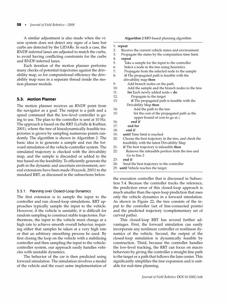
28 • Journal of Field Robotics—2008
A similar adjustment is also made when the vi-sion system does not detect any signs of a lane butcurbs are detected by the LIDARs. In such a case, theRNDF-inferred lanes are adjusted to match the curbs,to avoid having conflicting constraints for the curbsand RNDF-inferred lanes.
Each iteration of the motion planner performsmany checks of potential trajectories against the driv-ability map, so for computational efficiency the driv-ability map runs in a separate thread inside the mo-tion planner module.
5.3. Motion Planner
The motion planner receives an RNDF point fromthe navigator as a goal. The output is a path and aspeed command that the low-level controller is go-ing to use. The plan to the controller is sent at 10 Hz.The approach is based on the RRT (LaValle & Kuffner,2001), where the tree of kinodynamically feasible tra-jectories is grown by sampling numerous points ran-domly. The algorithm is shown in Algorithm 2. Thebasic idea is to generate a sample and run the for-ward simulation of the vehicle-controller system. Thesimulated trajectory is checked with the drivabilitymap, and the sample is discarded or added to thetree based on the feasibility. To efficiently generate thepath in the dynamic and uncertain environment, sev-eral extensions have been made (Frazzoli, 2001) to thestandard RRT, as discussed in the subsections below.
5.3.1. Planning over Closed-Loop Dynamics
The first extension is to sample the input to thecontroller and run closed-loop simulations. RRT ap-proaches typically sample the input to the vehicle.However, if the vehicle is unstable, it is difficult forrandom sampling to construct stable trajectories. Fur-thermore, the input to the vehicle must change at ahigh rate to achieve smooth overall behavior, requir-ing either that samples be taken at a very high rateor that an arbitrary smoothing process be used. Byfirst closing the loop on the vehicle with a stabilizingcontroller and then sampling the input to the vehicle-controller system, our approach easily handles vehi-cles with unstable dynamics.
The behavior of the car is then predicted usingforward simulation. The simulation involves a modelof the vehicle and the exact same implementation of
Algorithm 2 RRT-based planning algorithm
1: repeat2: Receive the current vehicle states and environment.3: Propagate the states by the computation time limit.4: repeat5: Take a sample for the input to the controller6: Select a node in the tree using heuristics7: Propagate from the selected node to the sample8: if The propagated path is feasible with the
drivability map then9: Add branch nodes on the path.10: Add the sample and the branch nodes to the tree.11: for Each newly added node v do12: Propagate to the target13: if The propagated path is feasible with the
Drivability Map then14: Add the path to the tree15: Set the cost of the propagated path as the
upper bound of cost-to-go at v
16: end if17: end for18: end if19: until Time limit is reached20: Choose the best trajectory in the tree, and check the
feasibility with the latest Drivability Map21: if The best trajectory is infeasible then22: Remove the infeasible portion from the tree and
Go to line 223: end if24: Send the best trajectory to the controller25: until Vehicle reaches the target.
the execution controller that is discussed in Subsec-tion 5.4. Because the controller tracks the reference,the prediction error of this closed-loop approach ismuch smaller than the open-loop prediction that usesonly the vehicle dynamics in a forward simulation.As shown in Figure 22, the tree consists of the in-put to the controller (set of line-connected points)and the predicted trajectory (complementary set ofcurved paths).
This closed-loop RRT has several further ad-vantages. First, the forward simulation can easilyincorporate any nonlinear controller or nonlinear dy-namics of the vehicle. Second, the output of theclosed-loop simulation is dynamically feasible byconstruction. Third, because the controller handlesthe low-level tracking, the RRT can focus on macrobehaviors by giving the controller a straight-line pathto the target or a path that follows the lane center. Thissignificantly simplifies the tree expansion and is suit-able for real-time planning.
Journal of Field Robotics DOI 10.1002/rob

Leonard et al.: A Perception-Driven Autonomous Urban Vehicle • 29
Figure 22. Illustration of RRT motion planning. Each leafof the tree represents a stopping location. The motion con-trol points (line-connected points) are translated into a pre-dicted path. The predicted paths are checked for drivability(curved paths).
5.3.2. Maintaining Safety as an Invariant Set
Ensuring the safety of the vehicle in a dynamic anduncertain environment is the key feature of our plan-ning system. Under normal driving conditions, oncea car comes to a stop, it can stay there for an indefiniteperiod of time and remain safe (Schouwenaars, How,& Feron, 2004). Using this stopped state as a safe in-variant state, our RRT requires that all the branchesin the tree end with a stopped state. The large cir-cles in Figure 22 show the stopping nodes in the tree,and each forward simulation terminates when the carcomes to a stop. The existence of the stopping nodesguarantees that there is always a feasible way to cometo a safe stop when the car is moving. Unless there isa safe stopping node at the end of the path, Talos doesnot start executing it.
5.3.3. Biased Sampling
Another extension to the RRT algorithm is that it usesthe physical and logical structure of the environment
0 5 10 15 20
10
0
5
10
15
20
Samplesσ line
(a) (b)
Figure 23. (a) Biased Gaussian samplings. The x, y axesare in meters. (b) Biased sampling for three-point turns:Talos shown in position after the first forward leg of theturn.
to bias the sampling. The samples are taken in twodimensions, and they are used to form the in-put to the steering controller. To take a sample(xsample,ysample), the following equation is used:
[xsampleysample
]=
[x0y0
]+ r
[cos θ
sin θ
],
r = σr |nr | + r0,
θ = σθnθ + θ0,
where nr and nθ are random variables that haveGaussian distributions, σr and σθ give the 1 − σ val-ues of the radial and circumferential direction, r0 andθ0 are the offsets, and (x0, y0) is the center of theGaussian cloud. Figure 23(a) shows 100 samples andthe 1 − σ lines, with the following parameter val-ues: σr = 10, σθ = π/4, r0 = 5, θ0 = π/3, and (x0, y0)= (0, 0). Different bias values are used based on thevehicle location, such as a lane, an intersection, ora parking lot. The situational information from thenavigator such as speed limits, passing allowed, andU-turn allowed, was also used to generate differentsampling biases.
Figure 23(b) shows the samples generated whiledesigning a U-turn maneuver. To perform generalN -point turns in cluttered environments, the sam-pling includes both the forward and reverse travelingdirections. A cone of forward samples is generatedto the left front of the vehicle to initiate the turn (itappears at the top left of the road shown). A set of re-verse samples is also generated, which appears to the
Journal of Field Robotics DOI 10.1002/rob

30 • Journal of Field Robotics—2008
right of the road shown. These samples will be usedafter executing the first forward leg of the turn. Then,another set of forward samples is generated to the leftof the current vehicle location (it appears at the bot-tom left of the road shown), for use when completingthe turn. For example, the parameter values used foreach of these three sets determining a U-turn ma-neuver are, respectively, σr1 = 8, σθ1 = π/10, r01 = 3,and θ01 = 4π/9; σr2 = 10, σθ2 = π/10, r02 = 5, andθ02 = −π/4; and σr3 = 12, σθ3 = π/10, r03 = 7, andθ03 = π . Samples for the first leg of the U-turn ma-neuver are positioned relative to the vehicle. Samplesfor each subsequent leg of the U-turn maneuver aredrawn with respect to the previous sample position.
The use of situational/environmental structurefor biasing significantly increases the probability ofgenerating feasible trajectories, making the RRT suit-able for the real-time applications. Team MIT useda single planner for the entire race, which showsthe flexibility and the extensibility of this planningalgorithm.
5.3.4. Lazy Reevaluation
In a dynamic and uncertain environment, the situa-tional awareness is constantly changing, but check-ing the feasibility of the entire tree against the lat-est drivability map is time consuming. The systemchecks the feasibility of the path when it is generated(Algorithm 2, line 8), but does not reevaluate itsfeasibility until it is selected as the best path to beexecuted (Algorithm 2, line 21). This “lazy check” ap-proach significantly reduced the time spent checkingthe feasibility using the drivability map but still en-sured that the path that was sent to the controller wasalways feasible with respect to the latest perceivedenvironment.
5.4. Controller
The controller takes the motion plan and generatesgas, brake, steering, and gear shift commands (col-lectively referred to as the control signals) that trackthe desired motion plan. The motion plan containsthe same information as the controller input usedin the planner prediction and consists of a list of(x, y) points that define the piecewise linear refer-ence path for the steering controller and the asso-ciated reference speed. The controller has two com-ponents: a pure-pursuit steering controller and theproportional–integral (PI) speed controller. A pure-
pursuit algorithm is used for steering control be-cause it has demonstrated excellent tracking perfor-mance for both ground and aerial vehicles over manyyears (Kelly & Stentz, 1997; Park, Deyst, & How,2007). A simple PI controller is implemented to trackthe commanded speed. These two core modules areembedded in the execution controller, but also withinthe motion planner for trajectory prediction, as dis-cussed in Subsection 5.3. The generated control sig-nals are sent to ADU for actuation, and the controllerloop runs at 25 Hz.
5.4.1. Steering Controller
The low-level steering control uses a modified ver-sion of the pure pursuit control law (Kelly & Stentz,1997; Park et al., 2007) to steer the vehicle along thedesired path. The steering control law is given by
δ = − tan−1(
L sin η
L1/2 + la cos η
),
where L is the constant vehicle wheelbase, la is theconstant distance between the pure pursuit anchorpoint and the rear axle, η is the angle between thevehicle heading and reference path direction, and L1is the look-ahead distance that determines how farahead on the reference path the controller shouldbe aiming. A smaller L1 produces a high-gain con-troller with better tracking performance. However,to ensure stability against the system delay, L1 mustbe enlarged with speed (Park et al., 2007). Figure 24plots the relation between the L1 and the commandedspeed. The L1 has a minimum value to ensure that thecontroller is stable at low speed. The L1 is also cappedfrom above, to ensure that the look-ahead point stayson a path within a reliable sensing range.
To improve trajectory tracking performance, thecontroller scales L1 as a function of the commandedspeed. Up to the time of the site visit in June 2007, L1was determined as a function of the measured vehi-cle speed. The result was that any error in the speedprediction would translate into a different L1 beingused by the motion planner prediction and the con-troller execution, which effectively changes the gainof the steering controller. In the final approach, theRRT planner determines the commanded speed pro-file, with the result that the speed and steering con-trollers are decoupled.
Journal of Field Robotics DOI 10.1002/rob

Leonard et al.: A Perception-Driven Autonomous Urban Vehicle • 31
0 2 4 6 8 100
2
4
6
8
10
12
speed command (m/s)
L1
dis
tan
ce (
m)
Figure 24. L1 distance as a function of the commandedspeed.
5.4.2. Speed Controller
The speed controller is a low-bandwidth controllerwith the following gains:
u = Kp(v − vref) + Ki
∫(v − vref)dt,
Kp = 0.2,
Ki = 0.04.
The output of the speed controller u is a normalizedvalue between −1 and +1. Using a piecewise lin-ear mapping shown in Figure 25, u is converted tothe voltage command to ADU. Note that the initialtesting revealed that the EMC vehicle interface hasa deadband between 1,850 and 3,200 mV. To achievea smooth coasting behavior, when the normalizedcontroller output is small, (i.e., |u| ≤ 0.05), no gas orbrake is applied. To skip the deadband and quicklyrespond to the controller command, the small posi-tive output (u = 0.05) corresponds to the upper limitof the deadband, 3,200 mV, and the small negativeoutput (u = −0.05) corresponds to the lower limit ofthe deadband, 1,850 mV.
To help reduce the prediction error, the com-manded speed is tied to the predicted vehicle loca-tion, rather than time. The time-based reference leadsto a coupling between the steering and speed con-trollers, even when L1 is scheduled as a function ofthe commanded speed. For example, if the actualvehicle speeds up slower than the prediction witha ramp-up speed command, the time-based speedcommand would make L1 larger than the predictedL1 when reaching the same position. This differ-
0 0.5 1
500
1000
1500
2000
2500
3000
3500
4000
4500
normalized controller output
volta
ge c
om
mand (
mV
)
Figure 25. Conversion from the speed controller output tothe ADU command voltage.
ence in L1 can lead to a significant steering error.The space-based reference makes the steering perfor-mance relatively insensitive to these types of speedprediction errors.
6. CHALLENGE RESULTS
To complete the DARPA Urban Challenge, Talos suc-cessfully negotiated first the NQE and then the raceitself. This section reviews the vehicle’s performancein these events.
6.1. NQE Performance
The NQE trials consisted of three test areas. Area Atested merging into traffic and turning across traf-fic. Area B tested navigation in suburban crescentsand parking and passing of stopped vehicles. Area Ctested intersection precedence and route blockage re-planning. The NQE was also the first chance to testTalos in a DARPA-designed course and RNDF. Onday 1 we were testing not only our ability to com-plete the mission but also the compatibility of coordi-nate systems and RNDF conventions. Team MIT com-pleted one mission a day for the first 3 days of thequalifier, with a five-mission endurance test on thefourth day, as shown in Table 1.
Successful negotiation of the NQE trials and,later, the race, required macro-level behavior tuningto manage trade-offs in uncertain scenarios:
• no progress due to a road blockage versus aperception failure (such as a misdetected curbcut)
Journal of Field Robotics DOI 10.1002/rob

32 • Journal of Field Robotics—2008
Table I. Results for all of Talos’s NQE tests.
Day Date NQE schedule Outcome
1 Sat. 27th Oct. Area B 1st trial Completed2 Sun. 28th Oct. Area C 1st trial Completed, but went around the roadblock3 Mon. 29th Oct. Area A 1st trial Completed: safe, but slow (7 laps in 24 min)4 Tues. 30th Oct. Area B 2nd trial Still progressing, but ran out of time
Area C 2nd trial Went off-road after 2nd K-turn at blockageArea A 2nd trial Completed: safe and faster (10 laps in 12 min)Area B 3rd trial CompletedArea C 3rd trial Completed after recovery from K-turn at first blockage
5 Wed. 31st Oct. —
• no progress due to a vehicle to queue behindand pass versus a perception failure (such asa lane positioning error)
• safe versus overly cautious behavior
After leaving the start chute, Talos was reluctantto leave the start zone. The boundary from the raisedstart zone into the challenge lane was in fact a 6-in.(15 cm) drop smoothed by a green ramp. This drop-off was detected by our vehicle as a ditch. Figure 26(a)shows how the drop-off appeared to our vehicle.Reluctant to drive down such a drop-off, the vehi-cle looked for an alternate route. Unable to makeprogress, the fail-safe logic eventually relaxed theconstraint that had been avoiding the ditch. The ve-hicle then drove down the challenge lane.
Figure 26(b) shows how our system relies on localperception to localize the RNDF map data. The laneahead of the vehicle is dilated, representing the po-tential ambiguity in where the lane may actually be.The dilation contracts to the lane position at certaincontrol points because of either a close GPS waypointor lane tracking.
During Talos’s first parking attempt, we struckthe first difference in the way Team MIT and DARPAinterpreted the RNDF. Figure 26(c) shows that thegoal point our vehicle is trying to drive to is underthe parked vehicle in front. For parking spots andother checkpoints, we attempted to get the vehiclecenter to cross the checkpoint. To achieve this, weplaced the goal location ahead of the checkpoint tomake the vehicle pass over the checkpoint. The posi-tioning of the vehicles and the parking spots indicatesthat DARPA simply required the vehicle to drive upto the checkpoint in this test. The sampling strategyof the RRT planner assumed that the parking spotwas empty. The blocked parking spot caused many
of the samples to be discarded because the last por-tion of the trajectory was infeasible. This is why Talosspent more than a minute in the parking zone. Forthe final race, a new sampling strategy was devel-oped that caused Talos to come as close to the check-point in the parking spot as possible, which can beperformed much more quickly. This figure also showssome transient phantom obstacle detections causedby dust in the gravel parking zone to the left ofTalos.
To ensure that Talos would queue behind a slow-moving vehicle yet still pass a stationary vehicle orobstacle, the system was designed to artificially chokeoff the road beside an obstacle in the lane. BecauseTalos could then not make progress, it would wait10 s to determine whether the obstacle was a vehi-cle moving slowly or a stationary object. If the objectremained still, Talos would begin a passing maneu-ver. In the gauntlet, this choke-off behavior misfired.Figure 26(d) shows our vehicle waiting to go intopassing mode beside a parked car. The road curva-ture causes the obstacle to appear more directly in ourlane than was actually the case. Stuck for a time be-tween the impassable regions generated from the ve-hicle on the right and a drivability map rendering ar-tifact on the left, Talos entered into the fail-safe modewith relaxed lane boundary constraints. Talos thensailed through the rest of the gauntlet and completedthe mission. Note that the parked cars and obsta-cles still appear as infeasible regions off-limits to thevehicle.
Area C tested intersection precedence and block-age replanning. The vehicle did very well at intersec-tion precedence handling in many different scenarios.Figure 27(a) shows Talos correctly giving precedenceto three traffic vehicles before going ahead of thesecond oncoming traffic vehicle. Figure 27(b) shows
Journal of Field Robotics DOI 10.1002/rob

Leonard et al.: A Perception-Driven Autonomous Urban Vehicle • 33
(a) (b)
(c) (d)
Figure 26. Area B first trial highlights. (a) Road-hazard map showing a line of hazardous terrain across the road at the endof the zone. The drop-off onto the challenge lane was detected as a ditch. (b) Lane position uncertainty between controlpoints reflected by lane dilation. The road past where Talos can perceive it is dilated, reflecting the potential ambiguity inlane position. (c) Parking goal position under car in front. (d) a virtual blockage used to enforce passing behavior causingundesired results.
Talos queueing behind a traffic vehicle before givingprecedence at the intersection.
Blockage replanning was more challenging. Taloscorrectly detected and stopped at the line of trafficbarrels [see Figure 27(c)], and then its programmingcaused it to try a passing attempt to drive aroundthe blockage. After a predetermined period duringwhich no progress was made, the system would re-lax some of the perception constraints (to account forthe possibility that the road position had been poorlyestimated, for example) or declare a blockage andturn around. At the time of this test, the logic wasset up to relax the lane constraints prior to declar-ing a blockage, assuming that a blockage would betruly impassable. Section 5.1.3 contains the logic.Figure 27(d) shows the perceived world once in fail-safe mode. Once the lane constraints were dropped,the route around the blockage was high cost, butpassable, so Talos drove around the blockage and fin-ished the mission.
The Area A trial was a merging test with human-driven traffic vehicles. Leading up to the trial, muchemphasis was placed on safety, so on the evening be-fore the trial Team MIT reexamined and tested thelogic used to determine when it was safe to merge.Increased caution and an unexpected consequence ofa bug fix prompted the increase of Talos’s safety mar-gin for merging from an 8-s window to a 13-s win-dow. As a result, during the Area A trial, Talos per-formed safely, but very cautiously, as it was waitingfor a 13-s window in the traffic, and such a windowrarely appeared. In the 24-min trial, Talos completedonly seven laps.
Figure 28(a) shows the vehicle track on the rightapproaching at 3.5 m/s despite being occluded by avehicle in the closer lane tracked by the radar andLIDAR as traveling at 3.9 and 4.3 m/s, respectively.
Although the fail-safe mode permitted Talos tocomplete the first Area B trial, the team decided tofix the bugs that led to Talos ending up in this mode
Journal of Field Robotics DOI 10.1002/rob

34 • Journal of Field Robotics—2008
(a) (b)
(c) (d)
Figure 27. Area C first trial highlights. (a) Intersection precedence with four traffic vehicles. (b) Queuing before an inter-section. (c) Attempting to go around a blockage. (d) Fail-safe mode 1 permits the vehicle to go around the blockage.
and use it only as a last resort. On the second trial atArea B, many of the bugs seen during the first trialwere fixed, including the dip leading out of the start
zone, the rendering artifact bug, and the parking spotlocation ahead of the checkpoint. However, a fewnew issues arose.
(a) (b)
Figure 28. Area A first trial highlights. (a) Vehicle approaching on the right is tracked despite being occluded by a closervehicle. (b) High traffic density makes for a long wait.
Journal of Field Robotics DOI 10.1002/rob

Leonard et al.: A Perception-Driven Autonomous Urban Vehicle • 35
(a) (b) (c) (d)
(e) (f)
Figure 29. Area B second trial highlights. (a), (b), (c), and (d) show a sequence of navigator plans. After a blockage isdeclared in the gauntlet, Talos attempts to reach the checkpoint from the opposite direction. (e) Talos gets stuck and cannotgo into passing mode due to a poor lane estimate resulting in the appearance that it was not entirely in its lane. (f) Thisblockage was real. Talos detects the blockage and completes a K-turn.
On its route through the gauntlet, Talos becamestuck due to a combination of a poor lane estimate,the virtual object used to force a passing behavior,and a bug that would not permit Talos to go intopassing mode if it was not fully within the estimatedlane, as shown in Figure 29(e). Eventually Talos madeno progress for long enough that a blockage was as-sumed. Talos then planned to turn around and ap-proach the checkpoint from the opposite direction.Figures 29(a) and 29(b) show the originally plannedroute and the alternate route through the gauntletfrom the opposite direction, respectively. Talos com-pleted the gauntlet in the opposite direction and thenneeded to turn around again to hit the original check-point. Figure 29(c) shows the intended route becausethe blockage now seems to have been removed. Enroute, Talos came across a legitimate road blockageshown in Figure 29(f). Talos completed a K-turn andexecuted the revised plan shown in Figure 29(d).
Talos continued to make progress, but given the extradistance traveled, it ran out of time before completingthe course.
During the second trial of Area C, the macro-behavior tuning had improved such that Taloscorrectly inserted a blockage and made a K-turninstead of simply driving around the blockage.However, during the second K-turn on the farside of the blockage, a poor lane estimate and arestricted region generated by obstacles perceived tobe in the lane conspired to stall progress [shown inFigure 30(a)]. Eventually, Talos entered fail-safemode and proceeded with relaxed lane constraintsand a reduced restricted region. Unfortunately, asTalos was driving out of a successful K-turn, theno-progress timer triggered and Talos reconsideredits blockage choice. Talos elected to block the currentpath and try the original route. In the recovery modeTalos was enabled to drive across curbs, behind the
Journal of Field Robotics DOI 10.1002/rob

36 • Journal of Field Robotics—2008
(a) (b)
Figure 30. Area C second trial highlights. (a) Progress is stalled during the second K-turn by a poor lane estimate and arestricted region. (b) Fail-safe mode is entered and would have permitted a successful K-turn, except that the goal locationnow reverts to the far side of the blockage.
DARPA observation tent and around the blockageto complete the mission [shown in Figure 30(b)]. TheDARPA officials intervened.
For the second trial of Area A, the safety marginfor merging (which, at 13 s, had caused a significantamount of waiting in the first trial) was reduced to9 s. The planning sequence was also modified so thatthe RRT planner could prepare paths for Talos to fol-low while the navigator waited for the crossing trafficto clear the intersection. This improved the responsetime of the vehicle, and the overall results were muchbetter, with 10 laps in just 12 min. Figure 31 shows a
photo of Talos and a screenshot of the viewer outputfor this mission.
Figure 32 illustrates Talos’s performance in itsArea B third trial. In the gauntlet, the artificial chokeon the road was removed, and passing was success-ful. Talos got stuck on curbs a few times, probablydue to inaccurate lane estimates, but otherwise exe-cuted the mission well.
A consequence of our decision to treat environ-mental perception as a higher authority than mapdata was that, at times, the lane estimate would snapto a new confident estimate. Some basic transitioning
(a) (b)
Figure 31. Area A second trial highlights. (a) Talos is looking for smaller gaps than in the first trial. (b) The RRT planner isworking while waiting for oncoming traffic to clear.
Journal of Field Robotics DOI 10.1002/rob

Leonard et al.: A Perception-Driven Autonomous Urban Vehicle • 37
(a) (b)
(c) (d)
Figure 32. Area B third trial highlights. (a) Without visual lane tracking, a curb-free space algorithm localizes the lane.(b) Visual lane tracking often recovers, providing an improved road estimate. (c) Without a virtual obstacle, passing willstill occur as long as the object occupies enough of the lane. Here the parked car still induces a passing behavior. (d) Oncein passing mode, parked cars are easily maneuvered around.
was implemented in the drivablility map to attemptto smooth the transition. In the best case the mo-tion planner would discover a new trajectory to thegoal within the next planning iteration. If no for-ward plan could be found, the vehicle would beginan emergency brake. Occasionally the vehicle wouldbe placed too close to detected curbs. Although thevehicle footprint is cleared of infeasible curbs, the ar-eas around the vehicle were not edited in this way. Ifcurbs impeded progress, the vehicle would become“ship wrecked.” After the no-progress timer got suf-ficiently high, the curbs were rendered as high costinstead of infeasible and the vehicle would proceed.Figures 32(a) and 32(b) show how the lane estimate
can shift based on new data. The problem is a con-sequence of limited development time. The intentionwas to use the detected curbs in the lane estimationprocess for the race. As described in Section 4.4, thecapability in the software was present, but unfortu-nately the integration was a little too immature to usein the race, so the simpler “curbs as obstacles” ap-proach was used.
Figure 33 illustrates Talos’s performance in itsArea C third trial. After correctly detecting the block-age, during the first K-turn, the vehicle drove off theroad and the pit crew was called to reposition the ve-hicle; after this intervention, Talos completed the mis-sion successfully.
Journal of Field Robotics DOI 10.1002/rob

38 • Journal of Field Robotics—2008
(a) (b)
Figure 33. Area C third trial highlights. After correctly detecting the blockage, Talos begins a K-turn. The navigator’splan changes. Talos enters fail-safe mode, drives off-road, and is recovered by the pit crew. (b) After the intervention, Talosresumes, and its second K-turn goes well.
6.2. UCE Performance
Overall, the team was very pleased with the perfor-mance of the vehicle during the race. Figure 34 showssome general highlights of Talos’s performance dur-ing the UCE. Figure 34(b) shows Talos driving downPhantom East. The vehicle speed was capped at25 mph as this was the highest speed for whichwe had validated our vehicle model. The radar inthe picture reads 24 mph. Figure 34(d) shows Ta-los queuing patiently behind a metal pipe gate thathad blown across an intersection safety region. Thegate was later forcefully removed by the DARPA offi-cials. After initially passing the Cornell chase vehicle,Figure 34(c) shows Talos slowing to merge safely be-hind the Cornell chase vehicle as the two-lane roadmerges back to one at the end of George Boulevard.Figure 34(e) shows an incident found while review-ing the logs. Talos correctly yields to a traffic vehicletraveling at more than 35 mph. The early detectionby Talos’s radar suite on the crescent road potentiallysaved the vehicle from a race-ending collision. Fi-nally, Figure 34(f) shows Talos crossing the finish lineafter completing the final mission.
The race consisted of three missions. Figure 35shows periods of no progress during the missions.An analysis of the peaks in these plots permits usto examine the principal failure modes during therace. During the first mission, fail-safe mode 1 wasentered twice, once at 750 s due to being stuck on
the wrong side of an artificial zone perimeter fence.Figure 36 shows how the lane next to the parkingzone is narrow in the RNDF (12 ft)—the actual lane isover 30 ft and extends into the zone. The lane percep-tion snaps to the real lane edge, trapping the vehicleagainst the zone boundary virtual fence. The secondfail-safe mode change came at 7,200 s due to a badlane estimate on a gravel road, which is discussed inSection 6.2.1. Several other times during this first mis-sion Talos was “ship wrecked” and made no progressfor 30 s until the curb constraints were relaxed. Inmission 2 the zone perimeter fence bug occurred at4,000 s. The third mission required three traversalsof the gravel road, which caused a large number of30-s intervals of no progress until curb constraintswere relaxed. Once at 7,200 s a bad lane estimate onthe gravel road caused Talos to enter fail-safe mode 1.
Outback Road was the Achilles’ heel of Talos’sUCE performance. We now examine the cause.
6.2.1. Outback Road
As noted above, Talos’s third mission during the UCErequired three traversals of the steep gravel roadknown as Outback Road. Figure 37 illustrates whythree traversals were required to hit the checkpoints.Of the 35 checkpoints in the mission, checkpoints 4,32, and 34 all required Talos to complete the one-way Outback, Phantom East circuit to hit the check-point and complete the mission. As far as we know,
Journal of Field Robotics DOI 10.1002/rob
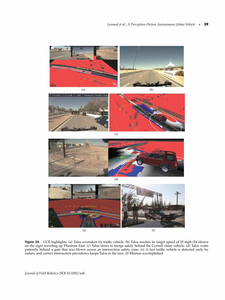
Leonard et al.: A Perception-Driven Autonomous Urban Vehicle • 39
(a) (b)
(c)
(d)
(e) (f)
Figure 34. UCE highlights. (a) Talos overtaken by traffic vehicle. (b) Talos reaches its target speed of 25 mph (24 shownon the sign) traveling up Phantom East. (c) Talos slows to merge safely behind the Cornell chase vehicle. (d) Talos waitspatiently behind a gate that was blown across an intersection safety zone. (e) A fast traffic vehicle is detected early byradars, and correct intersection precedence keeps Talos in the race. (f) Mission accomplished.
Journal of Field Robotics DOI 10.1002/rob

40 • Journal of Field Robotics—2008
0 2000 4000 6000 8000 10000 12000Time (sec)
0
10
20
30
40
50
60
70
80
90
Fails
afe
tim
er
(a) Mission 1
0 1000 2000 3000 4000 5000 6000Time (sec)
0
10
20
30
40
50
60
70
80
90
Fa
ilsa
fe t
ime
r
TimerPass, 15cm MarginReverse0cm Margin
Curbs drivableUn-Restrict goal
No Zone boundaries, No Standoffs
(b) Mission 2
0 2000 4000 6000 8000 10000 12000Time (sec)
0
10
20
30
40
50
60
70
80
90
Fa
ilsa
fe t
ime
r
TimerPass, 15cm MarginReverse0cm Margin
Curbs drivableUn-Restrict goal
No Zone boundaries, No Standoffs
(c) Mission 3
Figure 35. No-progress timer during the race. The timer is stalled during DARPA pauses. The X axis is the wall clock time.(a) During the first mission, fail-safe mode (80 s of no progress) is entered twice. 750 s: Zone perimeter fence bug. 7,200 s: Badlane estimate on gravel road. Other times Talos was “ship wrecked” and made no progress for 30 s until curb constraintswere relaxed. (b) Mission 2: 4,000 s; zone perimeter fence bug. (c) Mission 3: 7,200 s; bad lane estimate on gravel road. Manytimes during the three traversals of the gravel road section, no progress was made for 30 s until the curb constraints wererelaxed.
Journal of Field Robotics DOI 10.1002/rob

Leonard et al.: A Perception-Driven Autonomous Urban Vehicle • 41
Figure 36. Lane perception snaps the narrow (12 ft) RNDF lane to the (30 ft) actual lane boundary to the left (gray circles,lane centerline; white lines; lane boundary detections). The road would be drivable except that the zone virtual boundary(line to the left of the vehicle) extends into the physical lane blocking the road.
other teams were not required to complete this cir-cuit more than once. Figure 38 provides snapshotsof Talos’s performance while driving down the dirtroad; clearly, the system encountered difficulties onthis part of the course. The drop-off in the road pro-file was detected as a phantom curb or ditch. Whena steep section of road was directly ahead of Talos,the road-edge detector would occasionally detect thehill as a road edge. (As described in Section 4.3, theroad-edge detector was intended to detect berms aswell as curbs.) The road-edge system incorporated awork around designed to combat this problem: roadedges that were strongly perpendicular to the direc-tion of the road (as indicated by the RNDF) wereculled. We expected this feature to solve this prob-lem, but it did not. A flat road that curved only
in the direction of travel would be detected as aroad edge perpendicular to the road. However, thedirt road was crowned (had a side-to-side curva-ture), which caused the maximum curvature to ap-pear not to be directly across the travel lane and in-stead caused it to appear as two diagonal lines con-verging farther down the road. The slope of theselines was sufficiently parallel to the direction of travelthat they were not culled. Consequently, Talos wouldget stuck on the dirt road until a time-out elapsed (atwhich point the road edges were no longer treated asobstacles).
Again, as described earlier, the intended ap-proach of using the curb data in the lane estimate,if mature, would have gone a long way toward ad-dressing this problem.
Figure 37. To complete the third mission, three traversals of the Outback Road were required.
Journal of Field Robotics DOI 10.1002/rob

42 • Journal of Field Robotics—2008
(a) (b)
(c) (d)
(e) (f)
Figure 38. Steep gravel road. (a) and (b) Talos had no problem with gravel roads of gentle slope. (c) Roll-off of the gravelroad appears hazardous in the curb hazard map. (d) A phantom curb is detected at the road crest. (e) and (f) Phantom curbdetections contort the road corridor, choking the drivable region.
6.2.2. Collisions
Our vehicle had two incidents with Team CarOLO’svehicle “Caroline” during the UCE. In the first en-counter with Caroline, Talos paused as it enteredan intersection, following the process described inSection 5.1.1, and after resuming its forward motion,Caroline attempted to make a left turn directly acrossTalos’s path. The system initiated a “planner e-stop”just before DARPA issued a pause command to bothvehicles. These events are illustrated in Figure 39.
In a second incident with Team CarOLO’s vehi-cle, Talos was attempting to drive toward the zone
exit, between what appeared to be a fence on the leftand some static objects to the right. Caroline drove to-ward Talos, which applied hard braking but did notcome to a stop in time to avoid a collision. We do notknow why Caroline did not choose a path throughthe free space to Talos’s right, or why it continued toadvance when Talos was directly ahead of it. We hadmade a software architectural decision not to attemptto explicitly detect vehicles for the Challenge. Instead,Talos simply treated slow or stationary obstacles asstatic and faster moving obstacles as vehicles. Unfor-tunately Caroline’s speed, acceleration, stopping, and
Journal of Field Robotics DOI 10.1002/rob

Leonard et al.: A Perception-Driven Autonomous Urban Vehicle • 43
Figure 39. First Team CarOLO’s Caroline–Talos near miss.(a) Talos stops upon entering intersection. (b) Talos detectsthe moving object across its path and begins to plan a patharound it. (c) Talos begins an emergency stop. (d) Taloscomes to a stop. Caroline no longer appears to be movingand instead is viewed as a static object.
starting fell into a difficult region for our software. Ta-los treated Caroline as a static obstacle and was con-stantly replanning a path around it (to Talos’s left andCaroline’s right). Just before the collision, the systemexecuted “planner emergency stop” when Carolinegot sufficiently close. Unfortunately, due to Caroline’sspeed and trajectory, this could not prevent physicalcontact. These events are illustrated in Figure 40.
Talos’s collision with Cornell’s vehicle, Skynet,was another notable incident during the UCE andis illustrated in Figures 41 and 42. As described ear-lier in this report, Talos used a perception-dominatedsystem. It was designed to use the waypoints in theRNDF with limited confidence. Upon approachingthe intersection, Talos interpreted Skynet’s DARPAchase vehicle as being close enough to the road shoul-der to be a static feature (such as a tree or barrier onthe side of the road). Therefore, the road entry pointwas oriented to the left of the chase car. Talos droveup, gave way at the intersection, and then continuedto the left. Because Skynet and the chase car werestopped, Talos again interpreted them to be station-ary obstacles (such as K-rails). Talos drove throughthe intersection and was attempting to get back intothe exit lane when Skynet started to move. Againits speed was below Talos’s tolerance for treating itas a moving vehicle, and again Talos would haveavoided Skynet if it had remained stationary. As inthe collision with Caroline, Talos was applying emer-gency braking when it collided with Skynet. The rootcause was a failure to anticipate unexpected behav-ior from a stopped or slow-moving robot in a zone orintersection.
7. DISCUSSION
Overall, we were pleased with the performance ofour vehicle through the NQE and UCE competitions.By creating a general-purpose autonomous drivingsystem rather than a system tuned to the specifictest cases posed by DARPA, our team made substan-tial progress toward solving some of the underlyingproblems in autonomous urban driving. For example,in the NQE and UCE, there were a lot of traffic andintersection scenarios that we had never previouslytested, but the software was able to handle these sit-uations with little or no tweaking.
Our investment in creating a powerful new soft-ware architecture for this project paid off in innu-merable ways. The software developers devoted a
Journal of Field Robotics DOI 10.1002/rob

44 • Journal of Field Robotics—2008
Figure 40. Second Caroline–Talos incident. (a) Talos drives around the Caroline chase vehicle. (b) Talos drives aroundCaroline, which is moving sufficiently slowly to appear as a static object. (c) Talos continues to replan around Caroline,which was perceived as an static object in a different location. (d) Talos continues to drive around Caroline and then initiatesan emergency stop, but cannot stop in the space left and collides with Caroline.
significant amount of time to implementing a generic,robust software infrastructure for logging, playback,single-vehicle simulation, and visualization. Such aninvestment of energy would be hard to justify toachieve a single product such as a lane tracker or
an obstacle detector. However, the development androll-out of these innovations to support the wholeteam produced a more stable code base and enabledshared support of modules between developers aswell as quick and effective debugging.
Journal of Field Robotics DOI 10.1002/rob

Leonard et al.: A Perception-Driven Autonomous Urban Vehicle • 45
Figure 41. Lead-up to Skynet–Talos incident. (a) Talos initially queues behind the Skynet chase vehicle. (b) Lane positionis low, so Talos finds a route around the chase vehicle. (c) Talos yields at the intersection. There are no moving vehicles, soit proceeds through.
7.1. Perception-Driven Approach
For the final race, we added approximately 100waypoints such that our interpolation of the RNDFwaypoints more closely matched the aerial imageryprovided by DARPA. Our system was designed tohandle the original race description of perceiving andnavigating a road network with a sparse description,and Talos demonstrated its ability to do this by com-pleting the NQE without a densified RNDF. When itbecame apparent that this capability was not goingto be tested in the UCE, we added waypoints to im-prove our competitive chances. Nonetheless, duringthe UCE, Talos still gave precedence to perception-
based lane estimates over GPS and RNDF-derivedlanes, in accordance with our overall design strategy.
7.2. Slow-Moving Vehicles
Another key lesson learned was the difficulty ofdealing with slow-moving objects. We attempted toavoid the error-prone process of explicitly classify-ing obstacles as vehicles. Instead, our software han-dled the general classes of static obstacles and mov-ing obstacles. Although this strategy worked wellduring the NQE, in the race, the collisions or nearmisses involving Talos often came about due to the
Journal of Field Robotics DOI 10.1002/rob

46 • Journal of Field Robotics—2008
Figure 42. Skynet–Talos incident. (a) Talos plans a route around Skynet, which appears as a static object. (b) While Talos ispassing, Skynet begins to accelerate. (c) While applying emergency braking, Talos turns into the accelerating Skynet.
difficulty in handling changing traffic vehicle behav-ior or slow-moving traffic vehicles. Better handling ofslow-moving vehicles, for example through fusion ofvision and LIDAR cues to explicitly recognize vehi-cles versus other types of obstacles, is an avenue forfuture research.
7.3. Improved Simulation
Further investment in simulation tools for complexmultirobot interactions is warranted. For this project,we developed a useful simulation for a single roboticvehicle in a complex environment (including traffic
vehicles following predefined trajectories). We dis-cussed the possibility of developing a more complexsimulation that would enable us to test robot-against-robot (i.e., running our system “against itself”) butdecided against this endeavor due to time con-straints. In hindsight, this capability would have beenquite useful.
Whereas the vehicle generally operated in thevicinity of human-driven traffic without incident,problems were encountered when interacting withother autonomous vehicles at low speeds. These in-teractions likely arose due to some implicit assump-tions of our algorithms that were put in place to
Journal of Field Robotics DOI 10.1002/rob

Leonard et al.: A Perception-Driven Autonomous Urban Vehicle • 47
address the DARPA rules. These situations mighthave been detected from simulation of multiple au-tonomous vehicles running missions against eachother on the same course.
7.4. Verification of Fail-Safe Approaches
A key capability for long-term autonomous operationwas the creation of comprehensive fail-safe modes.The judicious use of fail-safe timers enabled the sys-tem to drop constraints and to free itself in difficultsituations, such as when perceptual estimates of thelane boundaries did not match reality. In any complexsystem of this type, the assumptions of the designerswill always be violated by unpredictable situations.The development and verification of more principledand robust approaches to recovering from mistakes isan important issue for robotics research.
8. RELEASE OF LOGS, VISUALIZATION,AND SOFTWARE
In the interest of building collaboration and astronger research base in the field, Team MIT hasmade its work available to the research community.The complete Talos UCE race logs, the viewer soft-ware, and video highlights from the race (made fromthe logs) are publicly available at
http://grandchallenge.mit.edu/public/
In addition, several core components developedfor the Urban Challenge have been released asopen-source software projects. The LightweightCommunications and Marshalling (LCM) softwarelibrary and the libcam image processing toolchainhave been released as open-source projects:
http://lcm.googlecode.com/http://libcam.googlecode.com/
These software components were described in Sec-tion 3.3.
9. CONCLUSION
This paper describes the developed software archi-tecture for a perception-driven autonomous urbanvehicle designed to compete in the 2007 DARPAUrban Challenge. The system used a comprehen-
sive perception system feeding into a powerful kino-dynamic motion planning algorithm to complete allautonomous maneuvers. This unified approach hasbeen “race proven,” completing the Urban Chal-lenge mission and driving autonomously for approx-imately 55 miles in under 6 h. A key novel as-pect of our system, in comparison to that of manyother teams, is that autonomous decisions were madebased on locally sensed perceptual data in preferenceto prespecified map data whenever possible. Our sys-tem was designed to handle the original race descrip-tion of perceiving and navigating a road networkwith a sparse description. Another innovative aspectof our approach is the use of a powerful and general-purpose RRT-based planning and control algorithm,achieving the requirements of driving in lanes, three-point turns, parking, and maneuvering throughobstacle fields with a single, unified approach. Oursystem was realized through the creation of a pow-erful new suite of software tools for autonomousvehicle research, tools that have been made avail-able to the research community. Team MIT’s innova-tions provide a strong platform for future research inautonomous driving in GPS-denied and highly dy-namic environments with poor a priori information.
ACKNOWLEDGMENTS
Sponsored by the Defense Advanced ResearchProjects Agency, Program: Urban Challenge, ARPAOrder No. W369/00, Program Code: DIRO. Issuedby DARPA/CMO under Contract No. HR0011-06-C-0149. Our team also gratefully acknowledges thesponsorship of the MIT School of Engineering, MITComputer Science and Artificial Intelligence Labora-tory (CSAIL), MIT Department of Aeronautics andAstronautics, MIT Department of Electrical Engi-neering and Computer Science, MIT Department ofMechanical Engineering, The C. S. Draper Labora-tory, Franklin W. Olin College of Engineering, TheFord–MIT Alliance, Land Rover, Quanta Computer,Inc., BAE Systems, MIT Lincoln Laboratory, MITInformation Services and Technology, South ShoreTri-Town Development Corporation, and AustraliaNational University. Additional support has beenprovided in the form of in-kind donations and sub-stantial discounts on equipment purchases from a va-riety of companies, including Nokia, Mobileye, Del-phi, Applanix, Drew Technologies, and AdvancedCircuits.
Journal of Field Robotics DOI 10.1002/rob
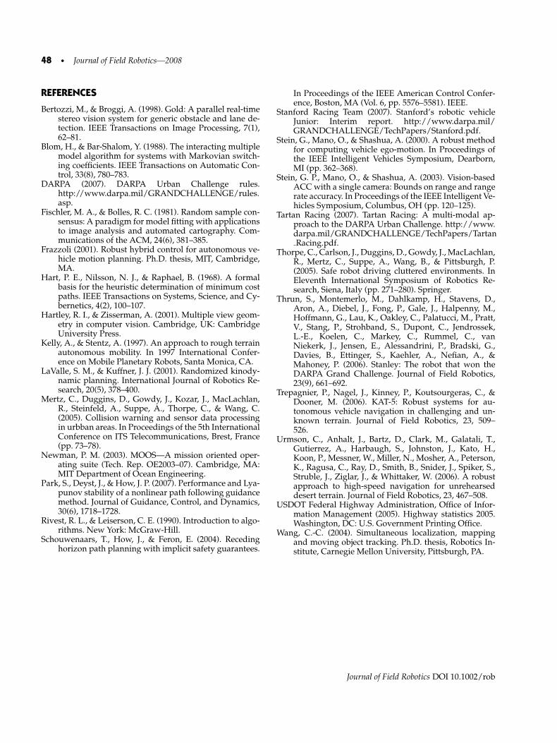
48 • Journal of Field Robotics—2008
REFERENCES
Bertozzi, M., & Broggi, A. (1998). Gold: A parallel real-timestereo vision system for generic obstacle and lane de-tection. IEEE Transactions on Image Processing, 7(1),62–81.
Blom, H., & Bar-Shalom, Y. (1988). The interacting multiplemodel algorithm for systems with Markovian switch-ing coefficients. IEEE Transactions on Automatic Con-trol, 33(8), 780–783.
DARPA (2007). DARPA Urban Challenge rules.http://www.darpa.mil/GRANDCHALLENGE/rules.asp.
Fischler, M. A., & Bolles, R. C. (1981). Random sample con-sensus: A paradigm for model fitting with applicationsto image analysis and automated cartography. Com-munications of the ACM, 24(6), 381–385.
Frazzoli (2001). Robust hybrid control for autonomous ve-hicle motion planning. Ph.D. thesis, MIT, Cambridge,MA.
Hart, P. E., Nilsson, N. J., & Raphael, B. (1968). A formalbasis for the heuristic determination of minimum costpaths. IEEE Transactions on Systems, Science, and Cy-bernetics, 4(2), 100–107.
Hartley, R. I., & Zisserman, A. (2001). Multiple view geom-etry in computer vision. Cambridge, UK: CambridgeUniversity Press.
Kelly, A., & Stentz, A. (1997). An approach to rough terrainautonomous mobility. In 1997 International Confer-ence on Mobile Planetary Robots, Santa Monica, CA.
LaValle, S. M., & Kuffner, J. J. (2001). Randomized kinody-namic planning. International Journal of Robotics Re-search, 20(5), 378–400.
Mertz, C., Duggins, D., Gowdy, J., Kozar, J., MacLachlan,R., Steinfeld, A., Suppe, A., Thorpe, C., & Wang, C.(2005). Collision warning and sensor data processingin urbban areas. In Proceedings of the 5th InternationalConference on ITS Telecommunications, Brest, France(pp. 73–78).
Newman, P. M. (2003). MOOS—A mission oriented oper-ating suite (Tech. Rep. OE2003–07). Cambridge, MA:MIT Department of Ocean Engineering.
Park, S., Deyst, J., & How, J. P. (2007). Performance and Lya-punov stability of a nonlinear path following guidancemethod. Journal of Guidance, Control, and Dynamics,30(6), 1718–1728.
Rivest, R. L., & Leiserson, C. E. (1990). Introduction to algo-rithms. New York: McGraw-Hill.
Schouwenaars, T., How, J., & Feron, E. (2004). Recedinghorizon path planning with implicit safety guarantees.
In Proceedings of the IEEE American Control Confer-ence, Boston, MA (Vol. 6, pp. 5576–5581). IEEE.
Stanford Racing Team (2007). Stanford’s robotic vehicleJunior: Interim report. http://www.darpa.mil/GRANDCHALLENGE/TechPapers/Stanford.pdf.
Stein, G., Mano, O., & Shashua, A. (2000). A robust methodfor computing vehicle ego-motion. In Proceedings ofthe IEEE Intelligent Vehicles Symposium, Dearborn,MI (pp. 362–368).
Stein, G. P., Mano, O., & Shashua, A. (2003). Vision-basedACC with a single camera: Bounds on range and rangerate accuracy. In Proceedings of the IEEE Intelligent Ve-hicles Symposium, Columbus, OH (pp. 120–125).
Tartan Racing (2007). Tartan Racing: A multi-modal ap-proach to the DARPA Urban Challenge. http://www.darpa.mil/GRANDCHALLENGE/TechPapers/TartanRacing.pdf.
Thorpe, C., Carlson, J., Duggins, D., Gowdy, J., MacLachlan,R., Mertz, C., Suppe, A., Wang, B., & Pittsburgh, P.(2005). Safe robot driving cluttered environments. InEleventh International Symposium of Robotics Re-search, Siena, Italy (pp. 271–280). Springer.
Thrun, S., Montemerlo, M., Dahlkamp, H., Stavens, D.,Aron, A., Diebel, J., Fong, P., Gale, J., Halpenny, M.,Hoffmann, G., Lau, K., Oakley, C., Palatucci, M., Pratt,V., Stang, P., Strohband, S., Dupont, C., Jendrossek,L.-E., Koelen, C., Markey, C., Rummel, C., vanNiekerk, J., Jensen, E., Alessandrini, P., Bradski, G.,Davies, B., Ettinger, S., Kaehler, A., Nefian, A., &Mahoney, P. (2006). Stanley: The robot that won theDARPA Grand Challenge. Journal of Field Robotics,23(9), 661–692.
Trepagnier, P., Nagel, J., Kinney, P., Koutsourgeras, C., &Dooner, M. (2006). KAT-5: Robust systems for au-tonomous vehicle navigation in challenging and un-known terrain. Journal of Field Robotics, 23, 509–526.
Urmson, C., Anhalt, J., Bartz, D., Clark, M., Galatali, T.,Gutierrez, A., Harbaugh, S., Johnston, J., Kato, H.,Koon, P., Messner, W., Miller, N., Mosher, A., Peterson,K., Ragusa, C., Ray, D., Smith, B., Snider, J., Spiker, S.,Struble, J., Ziglar, J., & Whittaker, W. (2006). A robustapproach to high-speed navigation for unrehearseddesert terrain. Journal of Field Robotics, 23, 467–508.
USDOT Federal Highway Administration, Office of Infor-mation Management (2005). Highway statistics 2005.Washington, DC: U.S. Government Printing Office.
Wang, C.-C. (2004). Simultaneous localization, mappingand moving object tracking. Ph.D. thesis, Robotics In-stitute, Carnegie Mellon University, Pittsburgh, PA.
Journal of Field Robotics DOI 10.1002/rob