A Parametric Case Study of the Apollo Program: Launch ...

1

A Parametric Case Study of the Apollo Program:

Launch Vehicle Sizing and Mission Architecture Selection

Mark D. Coley, Jr.,1 Kiarash Seyed Alavi,2 Ian W. Maynard,3 and Bernd Chudoba4

University of Texas at Arlington, Arlington, TX, 76019, U.S.A.

Vast amounts of Apollo documentation, both historical and technical in nature, has been

produced during the Apollo Program and after its closure. The records, however, indicate that

there is still a lack of an early-design phase physics-based parametric sizing quantification

tasked to enable correct holistic decisions from the outset towards program success. Historical

texts that explain the design decisions of Apollo do so in a predominantly qualitative manner,

leaving out the physics-based Future Projects Office type calculations. In contrast, technical

texts tend to explain the design details at high fidelity, overall leading the engineer away from

the big picture design understanding. Parametric quantification of key decisions made during

the Apollo Program would have allowed the future project engineers to identify the total

system solution space topography of feasible system designs and the total architecture. In

retrospect, parametric sizing studies do allow the modern decision-maker and engineer to

understand how the legacy Apollo Program could have been done better or if it already had

the best possible design choices implemented. What does the spacecraft look like for a given

mission architecture? How large does the launch vehicle need to be to complete that

spacecraft’s mission? How do the different options compare? This paper provides the

methods, analysis, and results to quantitatively answer these questions concerning the Apollo

Program. It also serves as the first validation case study for a prototype program planning

methodology and software implementation, Ariadne.

Nomenclature f = cost factor

g = gravity

Isp = specific impulse

m = mass

MR = mass ratio

n = number of stages

N = number of launches

NMF = net mass fraction

ΔV = velocity required

χ = split ratio

ϵ = structure factor

λ = payload fraction

I. Introduction HE Apollo Program is arguably the most famous space effort in the history of space exploration due to its overall

scale and what it managed to accomplish in such a short amount of time. This U.S. space program succeeded in

placing two men on the moon and returning them safely to Earth in 1969, only eight years after the first man had

ventured into space. Most people are familiar with the speech President Kennedy made to Congress in 1961: “… I believe that this nation should commit itself to achieving the goal, before this decade is out, of landing a man on the

moon and returning him safely to the earth. No single space project in this period will be more impressive to mankind, or

more important for the long-range exploration of space; and none will be so difficult or expensive to accomplish. We

propose to accelerate the development of the appropriate lunar space craft. We propose to develop alternate liquid and

1 PhD (graduated), AVD Laboratory, UT Arlington, AIAA Member. 2 PhD Candidate ([email protected]), AVD Laboratory, UT Arlington, AIAA Member. 3 PhD Candidate ([email protected]), AVD Laboratory, UT Arlington, AIAA Member. 4 Associate Professor ([email protected]), Director AVD Laboratory, UT Arlington, AIAA Member.

T

2

solid fuel boosters, much larger than any now being developed, until certain which is superior. We propose additional

funds for other engine development and for unmanned explorations—explorations which are particularly important for

one purpose which this nation will never overlook: the survival of the man who first makes this daring flight. But in a very

real sense, it will not be one man going to the moon—if we make this judgment affirmatively, it will be an entire nation.

For all of us must work to put him there. …” [1]

What most people do not remember is just how little the U.S. had accomplished in space at the time of that speech.

Less than three weeks before his speech, Alan Shepard became the first American in space on his sub-orbital flight in

a Project Mercury spacecraft. Yet, Kennedy still set the nation on a course to land two men on the Moon and return

them safely by the end of the decade. Figure 1 shows a timeline of the events leading up to the lunar landing. Along

the top of the figure are the more well-known milestones: Sputnik in 1957, Gagarin in 1961, etc., all the way to the

Apollo 11 lunar landing on July 20, 1969. The lower portion of the figure zooms in on a timeline of the years 1959

through 1963. This is when the decisions were made to land a man on the Moon in 1969; when multiple committees

tried to determine what path the U.S. space program should take. With his speech, Kennedy seized an opportunity to

overtake the Soviet space efforts with a manned lunar landing. After he committed the nation in May of 1961, it still

took over a year and the efforts of at least three different committees before a consensus was reached on how the

objective would even be accomplished.

Figure 1. A timeline depicting some of the key milestones in the US space program in the 1960s.

These early critical decisions are the ones that need to be investigated. How large a launch vehicle is required to

complete the desired objectives? What mission architecture should be used to accomplish this manned lunar landing?

This paper serves to illustrate how the Ariadne system (detailed in Refs. [2, 3]), the proposed solution concept of this

research, can be used to provide insight into such questions. The Ariadne system is a dedicated decision-support tool

developed for strategic planners. It is formally a space program planning methodology that integrates the top-level

spacefaring goals and program objectives of a space program with the lower-level mission architectures, hardware

elements, required future technologies, and current industry capability available at the time.

In order to demonstrate the contributions of the Ariadne prototype system, the U.S. space program as it led up to

The Apollo Program has been selected as the most significant case study. Twiss has the following to say about the

selection of an appropriate study: “… The choice of the first studies should also be considered carefully. Experience suggests that the following guidelines

are likely to provide a sound basis for their selection.

3

1. They should be limited in scope and conducted with data that are readily available using relatively simple

techniques.

2. Their results should be clear and unambiguous.

3. They should relate to a current technological problem of significance.

4. They should give support to a program advocated by an influential manager in the company. …” [4]

The Apollo Program fulfills each of his recommended guidelines. First, Apollo properly limits the scope for

analysis down to a single, albeit major, program for which there is an incredible amount of verification and validation

data from both historical and technical sources. The Ariadne prototype is also developed on the foundation of simple

methods integrated into a synthesis methodology. Second, the result of the present study, demonstrating the

significance of integrated decision support, will be clearly seen. Third, the case study directly relates to a current

problem as nations and organizations are challenged and often ill-prepared to correctly steer their space programs onto

a ‘best’ course forward (see Ref. [5] for a discussion of problems with current planning methods). Finally, Twiss’ last

point concerns establishing credibility when first introducing the solution to an audience unfamiliar with the approach.

The Apollo Program provides many opportunities to reverse-engineer the critical decisions of the space program to

first verify the process and then demonstrate the capabilities of the Ariadne solution at work.

Furthermore, the man-rated requirement of The Apollo Program provides the impetus for clearly defining the goals

and strategies involved in the years leading up to the lunar landing. General Dynamics, in their STAMP report, states: “… Of the two principal categories of operational space flight, namely manned and non-manned programs, the former is

by far the most expensive. It is, therefore, especially important to clearly define the objectives of manned

programs. …” [6]

Clearly defining objectives and how they are affected by early decisions is one of the primary deliverables of

the Ariadne system.

II. Ariadne Prototype Methods used in The Apollo Program Case Study For a walk-through of the (a) ideal Ariadne program planning methodology, and (b) the prototype methodology,

the reader is referred to Ref. [2] or [3]. The following section details the analysis methods used in the prototype

methodology that are not discussed in Ref. [2]. The following three sections specifically detail the methods for the

modeling and sizing of mission architectures and the sizing of launch vehicles and their respective cost.

A. Mission Architecture Modeling and Sizing of In-Space Elements

For the Ariadne prototype, the method for modeling

mission architectures is kept as basic as possible. Each

mission is divided into distinct phases*, assembling the

architecture in a way that can be easily analyzed with the

Tsiolkovsky rocket equation and mass ratio design

process. The first step in the architecture modeling

process requires a specified velocity requirement, ∆V, to

be determined for each phase. For this prototype, these

velocity requirements are based on conservative estimates

for similar maneuvers and not on actual calculated

trajectories that require a specific launch date, the precise

positions of the planetary bodies, etc. These velocity

requirements have been assembled from various sources and are listed in Table 1. The basic mentality of J. Houbolt†

was followed on the selection of the velocity requirements. Houbolt states: “ … It should be noted that a conservative approach has been taken in defining the velocity increments used in this study.

In general, non-optimum conditions have been assumed for each phase. While this approach tends to penalize the results

somewhat, it is considered to be the logical approach to a parametric study and contributes to the confidence in the results

obtained. …” [12]

In addition to the velocity requirements, two other inputs are required to enable the sizing of in-space elements: the

(a) propulsion performance (Isp), and (b) the structure factor (ϵ). Once defined, the IMLEO sizing process begins with

the final mission payload at its destination (actually, just before its final destination for the purposes of the prototype).

Beginning with the final mission payload, for example a satellite in geo-stationary orbit (GEO), the process applies

the rocket equation shown in Eq. (1), along with the known values for ∆V (change in velocity requirement), g

(gravitational constant), and the Isp (specific impulse) to solve for the mass ratio, MR, of the phase as seen in Eq. (2):

* Commonly referred to phases include the trans-Mars injection (TMI) and lunar orbit insertion (LOI). † Houbolt was the champion of the lunar-orbit rendezvous mission architecture used during project Apollo

Table 1. Velocity requirements of modeled phases for the

Ariadne prototype. Compiled and adapted from [7-11].

Mission Phase Velocity required [km/s]

Earth to LEO (185 km) 9.45

LEO to GEO (35,800 km) 4.95

LEO to lunar flyby 2.94

LEO to lunar orbit 3.88

LEO to lunar landing (soft, no return) 6.43

LEO to lunar landing and return 11.58

LEO to Mars flyby 3.61

4

Δ𝑉 = 𝑔𝐼𝑠𝑝(𝑀𝑅) = 𝑔𝐼𝑠𝑝 (𝑚0

𝑚𝑓

) (1)

𝑀𝑅 = 𝑒Δ𝑉

𝑔𝐼𝑠𝑝 (2)

Since MR = m0/mf , and the final mass at the end of the phase is the payload placed in orbit, the mass ratio and final

mass are multiplied together to determine the initial mass at the beginning of the phase which, in this case, is equal to

IMLEO. Other architectures might involve more phases, but the process is the same: simply start with the final mission

payload and solve for the initial mass at the beginning of that phase. This process is repeated for each subsequent

phase, using the output initial mass from the last phase as the input final mass for this phase. Hammond has this to say

about the use of similar equations to determine the final required in-space mass: “… The preceding close-form impulsive relations are only a preliminary estimating device, but should yield gross liftoff

weights within 10-15% of the actuals, depending upon the experience of the engineer in selecting mission velocity

requirement and estimating realistically achievable mass fractions. …” [13]

Additionally, with an assumed structure factor (ϵ) input for each phase, it is also possible to determine the

individual propellant and structure mass for each phase. The initial mass, m0, can be defined as

𝑚0 = 𝑚𝑠𝑡𝑟 + 𝑚𝑝 + 𝑚𝑝𝑎𝑦𝑙𝑜𝑎𝑑 (3)

where mstr is the structure mass of the stage, mp is the propellant mass and mpayload is the mass of the phase payload.

The final mass, mf, is defined as

𝑚𝑓 = 𝑚0 − 𝑚𝑝 = 𝑚𝑠𝑡𝑟 + 𝑚𝑝𝑎𝑦𝑙𝑜𝑎𝑑 (4)

The stage structure factor, ϵ, is an assumed input typically between 0.05 and 0.15 given by

𝜖 =𝑚𝑠𝑡𝑟

𝑚𝑠𝑡𝑟 + 𝑚𝑝

(5)

With this equation, it is now possible to solve for the propellant and structure mass required for each phase.

𝑚𝑠𝑡𝑟 =𝑚𝑝𝜖

(1 − 𝜖) (6)

𝑚𝑝 =𝑚𝑝𝑎𝑦𝑙𝑜𝑎𝑑(𝑀𝑅 − 1)

1 −𝑀𝑅𝜖

(1 − 𝜖)+

𝜖(1 − 𝜖)

(7)

These parameters in Eqs. (6) and (7) provide the details of the mass of a spacecraft (primarily its propellant

required) during a phase and the process can be used to determine the total IMLEO required for a given mission.

B. Sizing the Launch Vehicle

Once each mission has been reduced down to its IMLEO, a launch vehicle must be designed capable of delivering

that mass to orbit. As one of the primary drivers on both the cost and schedule of a program, the launch vehicle

requirements need to be easily comparable with a minimum of information needed. The launch vehicle sizing process

of the 1965 Space Planners Guide [14] provides that exact capability.

The Space Planners Guide (SPG) is a handbook method developed by the U.S. Air Force in the midst of the Space

Race. It states that its purpose is to “... provide a rapid means of both generating and evaluating space mission

concepts. …” [14]. The U.S. and the Soviet Union were each attempting to be the first to achieve increasingly difficult

milestones in space in an effort to prove their superiority.

Speed and first-order accuracy (or highest-of-importance accuracy) were critical to the Air Force in devising and

ruling out concepts during the early decision-making phase before countless resources were invested pursuing false

5

leads. The outcome has been a handbook methodology (SPG) that

allowed the decision-maker or subject-matter specialist alike to step

through nomograph-style figures in order to make their estimates. This

forgiving approach hides many of the second-order details from the

planner, thus it allows the user to see only the effects of the primary

drivers (gross design variables). The stated accuracy of the SPG is to be

within ± 20 %, which is sufficient for ruling out less practicable options.

This section will discuss Fig. 2 which is a N-S (Nassi-Shneiderman)

structogram representing the entire launch vehicle sizing process used

in the Space Planners Guide. The process involves three separate

sections: (1) the initial estimates of total and stage weights, (2) the

iteration of stage mass ratios in pursuit of velocity capability

convergence, and (3) the iteration of stage structure factors until the

optimized stage weights can be determined. For the sake of brevity, each

nomograph is not reproduced in this section.* The reader is encouraged

to follow along in Chapter V of the Space Planners Guide. The process

requires some basic inputs, many of which can be estimated from other

methods found in the SPG if they are unknown to the planner: the mass

of the payload, the number of stages, and some of the propulsion

properties of each stage (specific impulse† and propellant density). The

methods of the SPG primarily take the form of nomographs. Each

nomograph used in the process has been digitized to allow automation

and much faster application.

Following along with Fig. 2, the launch vehicle sizing structogram,

the planner first seeks to obtain a first estimate of the total launch vehicle

mass with nomograph V.C-9 and the average specific impulse of all the

stages and the number of stages (reproduced in Appendix, Fig. A.1). The

nomograph output is an estimate of the ratio of the launch vehicle total

mass to payload mass, which can be used to find the initial guess of the

launch vehicle’s overall mass. This ratio is the inverse of a commonly

used variable known as the payload fraction, λtotal, and will be expressed

as 1/λtotal for the sake of consistency. This is shown in Eq. (8):

𝑚𝑡𝑜𝑡𝑎𝑙 = 𝑚𝑝𝑎𝑦𝑙𝑜𝑎𝑑 × (1

𝜆𝑡𝑜𝑡𝑎𝑙

), (8)

where mtotal is the total lift-off mass of the launch vehicle, mpayload is the

payload mass and the inverse of the payload ratio, 1/λtotal, is the output

of nomograph V.C-9. With an estimate of the total launch mass, the

planner can then use nomograph V.C-10 to define the outer limits for

the basic dimensions of the launcher (reproduced in Appendix, Fig.

A.2). The nomograph provides an estimate for the maximum length and

diameter based on the total launch mass. These dimensions are not used

elsewhere in the process, but they could serve as initial constraints on

the launch site, manufacturing, support logistics, etc.

Continuing with the process, the inverse of the total payload ratio,

along with the number of stages, are used with nomograph V.C-11 to

determine the first estimate for the ratio of the stage mass to the mass

above the stage (reproduced in Appendix, Fig. A.3). This again, is the

inverse of the stage’s payload ratio, 1/λn. For the initial estimate, this

value is considered the same for each stage, but this will be optimized later in the process. Similarly, this stage’s

inverse payload ratio, the output of nomograph V.C-11, is used with nomograph V.C-12 (reproduced in Appendix,

* They can, however, be found reproduced in the Appendix from the Saturn IB case study. † Use the vacuum rating value.

Figure 2. N-S representation of the launch

vehicle sizing process from the Space

Planners Guide [14].

THE SPACE PLANNERS GUIDE

[LAUNCHER SIZING]

Input: number of stages, mpayload, mescape tower, ΔVreq,

propulsion properties of each stage (Isp, propellant

density)

Estimate total launch vehicle mass to payload

mass ratio – Figure V. C-9: (1/λtotal)

Until εn,old εn,new

Estimate stage mass to mass above stage

ratio – Figure V. C-11: (1/λn)

First estimate of mass ratio for each stage –

Figure V. C-11: MRn

Calculate first estimate of stage mass and total

mass of each stage: mtotal,n, mn

Estimate stage structure factor –

Figure V. C-15: ε1

First stage

Figure V. C-16: ε2

Second stage (if applicable)

Figure V. C-17: ε3

Third stage (if applicable)

Until ΔVcapability ΔVreq

Input: MRn

Estimate mass ratio for next stage –

Figure V. C-22: MRn+1

Estimate velocity capability of each stage –

Figure V. C-23: ΔVcapability,n

Calculate total velocity capability: ΔVcapability

Re-estimate stage mass to mass above stage

ratio – Figure V. C-24: (1/λn)

Re-estimate structure factor for each stage –

Figure V. C-15, C-16, and C-17: εn,new

Calculate final masses of launch vehicle:

mtotal,2, m2, mtotal,1, m1

Calculate stage masses of launch vehicle:

mtotal,2, m2, mtotal,1, m1

Estimate maximum length and diameter –

Figure V. C-10: l, d

6

Fig. A.4) to obtain the first estimate for the mass ratio* of each stage (again considered equal for now but will be

optimized later).

Using all the output values from nomographs V.C-9 through V.C-12, the planner can now determine the first

estimate of the stage masses. Simply begin with the payload mass and multiply it by the ratio obtained from nomograph

V.C-11, 1/λn. The SPG refers to this mass as the gross weight of the stage, which includes the mass of the stage (both

propellant and structure) and the mass above the stage though from here on out it will be referred to as the total mass.

In order to find just the mass of the stage, the planner can subtract the mass above the stage from the stage total mass.

This process can be seen for a two-stage launch vehicle in the following equations:

𝑚𝑡𝑜𝑡𝑎𝑙,2 = 𝑚𝑝𝑎𝑦𝑙𝑜𝑎𝑑 × (1

𝜆2

) (9)

𝑚2 = 𝑚𝑡𝑜𝑡𝑎𝑙,2 − 𝑚𝑝𝑎𝑦𝑙𝑜𝑎𝑑 (10)

𝑚𝑡𝑜𝑡𝑎𝑙,1 = 𝑚𝑡𝑜𝑡𝑎𝑙,2 × (1

𝜆1) (11)

𝑚1 = 𝑚𝑡𝑜𝑡𝑎𝑙,1 − 𝑚𝑡𝑜𝑡𝑎𝑙,2 (12)

where mtotal,n is the total mass of the nth stage (including the mass above it), mn is the stage mass of the nth stage (without

the mass above it), and 1/λn is the stage mass to mass above ratio that was found in nomograph V.C-11.†

The planner can repeat this process for each stage, starting with the last stage (second or third, depending on the

design) until he arrives at the final launch mass, which should be similar‡ to the total launch mass found with

nomograph V.C-9. The final portion of this initial estimate involves the recently determined stage masses and

propellant density to estimate the stage’s structure factor. The Space Planners Guide provides nomographs for stages

one, two, and three for both liquid or solid propellants.§ The SPG assumes an initial thrust-to-weight ratio for stages

one, two, and three of 1.3, 1.0, and 0.75, respectively. With the estimated structure factors, the structure and propellant

masses can be determined for each stage using Eqs. (13) and (14):

𝑚𝑠𝑡𝑟𝑢𝑐𝑡𝑢𝑟𝑒 = 𝑚𝑛 × 𝜖𝑛 (13)

𝑚𝑝𝑟𝑜𝑝𝑒𝑙𝑙𝑎𝑛𝑡 = 𝑚𝑛 × (1 − 𝜖𝑛) (14)

The next portion of the sizing process involves the iteration of the mass ratios of each stage and the determination

of the velocity contribution they are capable of providing. The velocity of each stage is then summed and compared

to the total velocity required. Nomograph C.V-22 is used to determine the mass ratio of each stage (reproduced in

Appendix, Fig. A.7). The planner enters the nomograph with a guess for the mass ratio of the first stage (from the

previous estimation for the first iteration). The structure factor and specific impulse of the stage are used, along with

the structure factor and specific impulse of the next stage to determine the stage mass ratio of that stage. This can be

repeated for a third stage by entering the nomograph with the second mass ratio to determine the third.

The mass ratio and specific impulse for each stage is then used with nomograph V.C-23 to estimate the velocity

contribution of the stage (reproduced in Appendix, Fig. A.8). Velocities are summed, then compared to the total

velocity required. If the velocity capability is too low, the planner increases their guess for the mass ratio of the first

stage and returns to nomograph V.C-22. If the velocity capability is too great, the guess is decreased. This is repeated

until the velocity capability converges with the velocity required.

* Where the mass ratio is defined as the ratio of the initial mass over the final mass. † Remember that 1/λ1 = 1/λ2 for this initial estimate. ‡ Opposing methods from the SPG may often differ slightly when the values are expected to be identical. This is

completely normal and aligns perfectly with the philosophy of the SPG. § For the development of the prototype, all liquid stages have been assumed so that only nomographs V.C-15 through

V.C-17 have been digitized. See reproduction for the first and second stages in Figs. A.5 and A.6.

7

Once the velocity capabilities have converged* with those required, the stage mass ratios are passed into

nomograph V.C-24 along with the structure factor of the stage to determine the new estimate for the stage mass to

mass above the stage ratio (reproduced in Appendix, Fig. A.9). These ratios can then be used like they were in the

first section of this process (see Eqs. (9)-(12)) to determine the individual stage masses, this time with the optimized

ratios, starting with the last stage. The individual stage masses are used again with nomographs V.C-15 through V.C-

17 to arrive at a new value for the stage’s structure factor. The planner then compares these new structure factors with

the original. If the difference is too large, the planner re-enters nomograph V.C-24 with the stage mass ratios and the

new structure factors for each stage. The stage masses are calculated again, followed by the stage structure factors.

This continues until the new and old structure factor values have converged. Once they have converged, the planner

has successfully sized the required launch vehicle for his given mission.

C. Launch Vehicle Cost Estimation

With the sizing data for each launch vehicle, it is then desired to be able to estimate the required costs for the

development and production of the required number of launch vehicles for each program. In order to make these

estimates, D. E. Koelle’s Handbook of Cost Engineering and Design of Space Transportation Systems with TransCost

8.2 Model Description [15] has been applied. Based on the book sales worldwide, Koelle states that “... this seems to

be the most widely used tool for cost estimation and cost engineering in the space transportation area [15]. TransCost

was also used at the beginning of the joint DARPA-NASA effort, the Horizontal Launch Study [16, 17].†

The TransCost handbook provides several different types of cost estimates: development costs, production costs,

ground and operations costs, and complete life cycle costs. For the prototype and the amount of launch vehicle data

that is available from the sizing process, only the development and production costs are calculated using cost

estimating relationships (CER). Koelle reports all of his estimated costs in the unit ‘work-years’ (WYr) which is

defined as “… the total company annual budget divided by the number of productive full-time people.” [15]. These

values can be converted to actual currency with a conversion factor that Koelle lists per year and per region. The latest

conversion factor is for the year 2015, so all reported costs will be in $2015. The conversion factor is given as 337,100

[$/WYr].

Koelle defines and uses 12 different cost factors, f0 – f11 that are combined with the CERs to estimate the required

costs for engines and vehicles. For the prototype, as the objective is to make comparisons at the top-level, many of

these factors can be ignored. They become critical when comparing alternative launch methods, which would be

included in the ideal solution concept, so they are not forgotten. The factors that have been included in the Ariadne

prototype are listed below:

• f0 – project systems engineering and integration factor;

• f1 – technical development standard correlation factor;

• f2 – technical quality correlation factor;

• f6 – cost growth factor for deviation from the optimum schedule.

These factors and the CERs for both engines and stages are discussed next. To estimate the total development cost

for a launch vehicle, the following equation is used:

Total development cost = 𝑓0(ΣEngine dev + ΣVehicle dev)𝑓6𝑓7𝑓8 (15)

where f0 is the systems engineering factor based on the number of stages (see below), and f6 is cost growth based on

schedule. The factors f7 and f8 are assumed to be equal to 1.0 for the purposes of the prototype. The systems engineering

factor for development is given as

𝑓0 = 1.04𝑛 (16)

where n represents the number of stages for the launch vehicle. The factor f1 is development standard factor. Its

standard values and their connections to the Ariadne technology strategy factor are provided in Table 2. The factor f2

is defined separately for each system and will be discussed when applicable. The factor f6 is based on the schedule of

* The SPG stresses not to pursue extreme accuracy in matching these values, “… since the accuracy of the solution is

already limited by the approximation of the input data. …” [14]. Since it is digitized and iterations can happen very

quickly now, the prototype does require a fairly close match, but it is important to remember the amount of

approximations already involved. † TransCost is eventually replaced with NAFCOM due to its ability to estimate DDT&E and first unit costs at the

subsystem level, which is very important for the study, but not necessary for the Ariadne prototype.

8

development. Typical development schedules based on the total number of WYr of the launch vehicle are suggested

by Koelle. For the purposes of the prototype:

• the assumed development time for launch vehicle under 15,000 WYr is 6 years;

• between 15,000 and 35,000 WYr is 7 years;

• and over 35,000 WYr is 8 years.

Table 2. Connection between Ariadne technology strategy factor and TransCost

development standard factor. TransCost descriptions reproduced from Koelle

[15].

Stech Description f1

1 Variation of an existing project 0.3 – 0.5

2 Design modifications of existing systems 0.6 – 0.8

3 Standard projects, state-of-the-art 0.9 – 1.1

4 New design with some new technical and/or operational features 1.1 – 1.2

5 First generation system, new concept approach, involving new

techniques and new technologies 1.3 – 1.4

These ideal values are compared with an assumed actual value for the development of each launch vehicle (based

on the Stime strategy factor). The relative difference between the two is used along with a digitized figure by Koelle in

order to determine the value of f6 for each launch vehicle. The development costs for pump-fed rocket engines is given

by

Liquid engine dev cost = 277𝑚0.48𝑓1𝑓2𝑓3𝑓8 (17)

where m is the mass of the engine, f2 is based on the number of test fires (and can be assumed equal to 1.0 for now), f3

and f8 are not applicable and also assumed to be 1.0. To determine the mass of the required engine, the total thrust of

each stage from the sizing output is split by a selected number of engines. Koelle provides a figure based on a database

of rocket engines that allows the user to estimate the engine’s mass for use in Equation (17). The development costs

for expendable vehicle stages is given by

Expendable stage = 98.5𝑚0.55𝑓1𝑓2𝑓3𝑓8𝑓10𝑓11 (18)

where m is the stage mass, f2 is based on vehicle net mass fraction (NMF) defined below, f10 and f11 can be assumed

equal to 1.0. Koelle defines the NMF as:

𝑁𝑀𝐹 =𝑚𝑠𝑡𝑎𝑔𝑒,𝑑𝑟𝑦𝑚𝑒𝑛𝑔𝑖𝑛𝑒𝑠

𝑚𝑝𝑟𝑜𝑝𝑒𝑙𝑙𝑎𝑛𝑡

(19)

The equation for f2 for expendable stages is then given by

𝑓2 =𝑁𝑀𝐹𝑟𝑒𝑓

𝑁𝑀𝐹𝑒𝑓𝑓

(20)

where NMFref is the average NMF value based on a database of launch vehicles for a given propellant mass, and

NMFeff is the calculated NMF value based on the sized launch vehicle stage and engine masses. Koelle’s handbook

contains many other CERs applicable to a wide range of vehicle types, but only expendable launchers with liquid

engines have been implemented for the prototype. The plot for each of these CERs for the estimation of development

costs has been compiled by Sforza [18] and reproduced in Fig. 3.

To estimate the total production cost for a launch vehicle, the following equation is used

𝑇𝑜𝑡𝑎𝑙 𝑝𝑟𝑜𝑑𝑢𝑐𝑡𝑖𝑜𝑛 𝑐𝑜𝑠𝑡 = 𝑓0𝑛 (∑ 𝑠𝑡𝑎𝑔𝑒 𝑝𝑟𝑜𝑑𝑢𝑐𝑡𝑖𝑜𝑛

𝑗

1

+ ∑ 𝑒𝑛𝑔𝑖𝑛𝑒 𝑝𝑟𝑜𝑑𝑢𝑐𝑡𝑖𝑜𝑛

𝑗

1

) 𝑓9 (21)

9

where n is the number of stages or system elements, j is the number of identical units per element, and f9 is not

applicable to the prototype and assumed to be 1.0.

Figure 3. Summary figure of the development costs for elements of a space

transportation system [15, 18].

Again, the prototype only involves expendable stages and liquid rocket engines. The production costs for liquid

rocket engines are given with the following two equations:

(Cryo)Engine Production cost = 3.15𝑚0.535𝑓4𝑓8𝑓10𝑓11 (22)

(Storable)Engine Production cost = 1.9𝑚0.535𝑓4𝑓8𝑓10𝑓11 (23)

where m is the engine mass, and the only other variable that has not been discussed is f4, the cost reduction factor for

series production. This factor is not applied in the prototype although it is a promising candidate for future work. The

CERs for expendable stages are given by the following two equations, also divided by cryogenic propellants and

storable propellants:

(Cryo)Stage Production cost = 1.84𝑚0.59𝑓4𝑓8𝑓10𝑓11

(24)

(Storable)Stage Production cost

= 1.265𝑚0.59𝑓4𝑓8𝑓10𝑓11 (25)

The plot for the production costs for

these stages and engines, along with other

types of systems can be seen in Fig. 4. With

these CERs in place, the Ariadne prototype

system is now able to calculate both

development and production costs of the

fleet of launch vehicles required to place the

program IMLEO into orbit. This process is

key to the program convergence loop as

previously discussed and shown in Fig. 4.

III. Sizing the Required Launch Vehicles This section serves to validate the application of the Space Planners Guide (SPG) to sizing launch vehicles. It

begins with an introduction to the family of launch vehicles that were developed for The Apollo Program: specifically,

the Saturn IB and Saturn V. Then, a walk-through of the sizing process to estimate the launch vehicle required for a

Figure 4. Summary figure of the production costs for elements of a space

transportation system. [18]

10

mission similar to that of the Saturn IB is presented. A walk-through of the process with Saturn V is not presented, as

the SPG’s sizing process optimizes the stages of a launch vehicle for a mission to a 185 km orbit. The actual Saturn V

used two full stages (S–IC and S–II) and only a partial burn of the third stage (S–IVB) to reach orbit. After some

diagnostics in LEO, the third stage was then re-ignited for the trans-lunar injection burn. Thus, the Saturn IB more

closely resembles the mission modeled by the SPG, though with some tweaking of the assumptions, the planner can,

in fact, reach a respectable estimate for the overall Saturn V launch mass. The historical values and the SPG estimated

launch vehicle are then compared and discussed. The results of the sizing process for a launch vehicle similar to the

Saturn V are then presented and discussed.

A. Introduction to the Saturn Family of Launch Vehicles

The Saturn launch vehicle development program was officially established on December 31, 1959. Within a month

it was designated as one of the highest priorities of the nation. The Saturn family of launch vehicles were to be

developed as a building block concept: elements (stages and engines) first developed for an initial launch vehicle

could be directly applied to subsequent stages as the program increased their capability and developed larger launch

vehicles [19]. There were at least seven planned Saturn configurations from the C-1 all the way up a possible C-8 [20,

21]. As goals became clearer and payload estimates more realistic, only three configurations emerged from the Saturn

program: the Saturn I, Saturn IB, and the Saturn V.*

B. Sizing Demonstration with the Saturn IB

The digitized Space Planners Guide sizing process

from the Ariadne prototype system is applied here to

estimate the launch vehicle required to perform a

mission similar to the Saturn IB to illustrate the utility

of the SPG and to help validate the results of the

process. The required inputs, assumptions, and final

deliverables are all provided.

1. First Section

To begin the sizing process, a number of inputs

must be supplied. Table 3 contains all the input data

required for the Saturn IB. The mission of the Saturn IB

was to launch to low Earth orbit to test out many of the

components and systems that would be required for the

future lunar landing. Including an assumption of the

velocity losses due to drag and gravity, the total

velocity required for its mission is about 9,450 m/s. For

the input characteristics of the propulsion systems, the

selected specific impulse values are the vacuum rating

reported for the Rocketdyne H-1 and J-2. The initial

thrust-to-weight ratios are suggested assumptions by

the SPG and also supported by Koelle and Thomae [22].

The first step is to find a rough estimate of the launch vehicle mass. With an average specific impulse of 357.7

sec., Fig. A.1 estimates the total launch vehicle mass to payload mass ratio (1/λtotal) to be 32.7. Equation (8) can then

be used to find the total mass of 608,220 kg.† With total mass and Fig. A.2, the maximum expected values of diameter

and length of the launch vehicle are determined to be 6.3 m and 47.4 m, respectively. Note that these dimensions are

not needed for further analysis.

The next step is to get a first estimate of the stage gross weight to weight above the stage ratio (1/λn) using Fig.

A.3 and the number of stages. The input of 32.7 produces a 1/λn ratio of 5.6. This value will initially be used for both

* Though, subsequent derivatives of the Saturn V were also under investigation; some even prior to the first launch of

the Saturn V. [14, 22] † Later, when comparing the estimated values with the historical values, it will be seen that this initial estimate is very

close for the Saturn IB. This should not come as a surprise, as the SPG’s nomographs were probably generated with

some of the data from the Saturn launchers and the Saturn IB flew the exact mission under consideration by the SPG.

This use of this nomograph alone does not hold up, however, for all launch vehicles, especially not more recent efforts.

Table 3. Listing the required inputs for the sizing

process and the values selected for the Saturn IB.

Compiled from multiple sources [23-25].

Inputs required

Destination LEO*

Payload mass 18,600 [kg]

Escape tower mass 4,000 [kg]

Number of stages 2

Propellant of each stage†

first RP-1/LOX

second LH2/LOX

Isp of each stage‡

first 296 [s]

second 419 [s]

Thrust-to-weight ratio

first 1.3

second 1.0 * 185 [km] orbit † used in determining the bulk density of the propellant ‡ using the vacuum rating

11

stages to determine the initial estimates of the

individual stage masses. The stage ratios will be

optimized in the second half of the sizing process.

Using Fig. A.4, the stage mass ratio (MRn) can be

determined. The stage mass to mass above the stage

ratio of 5.6 is used, resulting in an initial estimate of the

mass ratio, (MR), of 3.99 for both stages. Again, this

assumption of equal ratios for each stage will be

corrected in the second half of the process. These stage

ratios, along with the previously discussed Eqs. (9)

through (12), provide the initial estimate of the

contributing masses of each stage. The next two

figures, Figs. A.5 and A.6, are used along with the

newly estimated stage masses to determine the structure

factor for each stage. With the stage masses and structure factors estimated, the specific masses of the propellant and

structure of each stage can be found with Eqs. (13) and (14). The result of the first estimation for Saturn 1B is presented

in Table 4.

2. Second Section

This section of the sizing process attempts to optimize the mass of each stage to reach the target orbit and ΔVrequired

while minimizing the mass of the launch vehicle. Figure A.7 is then used to calculate the optimum stage mass ratio (it

shows the final iterated value). Now, with the mass ratio, MRn of each stage, the velocity capability of stage n is

determined with Fig. A.8. The initial mass ratio is adjusted until the velocity capability and the velocity required are

sufficiently close.*

3. Third Section

Once the ΔVs are converged, Fig. A.9 is used to calculate a new estimate of stage mass to mass above the stage

ratio (1/λn). Figures A.5 and A.6 are then used again to calculate the structure factors and then the process will iterate

until 𝜖𝑜𝑙𝑑 = 𝜖𝑛𝑒𝑤 . When converged, the final mass breakdown of each stage and overall launch vehicle can be

calculated. In summary, the SPG has been used to make two estimates for the masses of the Saturn IB: an initial

estimate that assumes equal stages mass ratios, and a final estimate that optimizes the launch vehicle for the minimum

launcher mass required to place the desired payload in a 185 km orbit.

Table 5. Comparison of sizing results with the actual Saturn 1B

Saturn 1B Actual First estimate % Error Final estimate % Error

Velocity capability, m/s 9,450 - - 9,465 0.01

Payload mass, kg 18,600 18,600 - 18,600 -

Escape tower mass, kg 4,000 - - 4,000 -

Second stage

Stage mass, kg 116,500 85,913 -27 117,998 2

Propellant mass, kg 105,300 77,150 -27 106,317 2

Structure mass, kg 10,600 8,763 -18 11,682 11

Total mass, kg 135,100 104,513 -23 136,598 2

First stage

Stage mass, kg 452,300 482,747 5 539,083 18

Propellant mass, kg 414,000 450,403 7 502,965 20

Structure mass, kg 40,500 32,344 -22 36,119 -13

Total mass, kg 587,900 587,261 -1 675,682 15

Table 5 shows the historical masses of the actual Saturn IB along with both estimates and the percent error of the

estimate. As can be seen, both estimates do an excellent job of estimating the mass of the total launch vehicle with

very little information. For the Saturn IB, the initial estimate is closer than the optimized estimate. This does not

suggest, however, that a planner should only use the first estimation method for any desired studies efforts. The final

estimate is still within the target accuracy of the SPG, and it fairs much better on the individual masses of the second

stage. As mentioned before, the initial estimate also comes from nomographs built upon data from launch vehicles

* A percent difference of 0.5% of the velocity has been used.

Table 4. The estimated values for the Saturn 1B from first

portion of the SPG sizing process.

First Estimate – Saturn 1B Variable Value [kg]

Payload mass 𝑚𝑝𝑎𝑦𝑙𝑜𝑎𝑑 18,600

Second stage

Stage mass 𝑚2 85,913

Propellant mass 𝑚𝑝,2 77,150

Structure mass 𝑚𝑠,2 8,763

Total mass 𝑚𝑡𝑜𝑡𝑎𝑙,2 104,513

First stage

Stage mass 𝑚1 482,747

Propellant mass 𝑚𝑝,1 450,403

Structure mass 𝑚𝑠,1 32,344

Total mass 𝑚𝑡𝑜𝑡𝑎𝑙,1 587,261

12

that existed at the time of the SPG’s development for a similar mission. This likely includes the Saturn IB, which

explains its accuracy.

C. Results of Sizing the Saturn V

The primary reason for using the Saturn IB for the walk-through is that its mission more closely mirrored the

‘default’ capabilities of the SPG sizing process: namely a multi-stage launch vehicle optimized to reach LEO. The

real Saturn V did in fact launch to a similar orbit, but it did so using two full stages and a partial burn of its third stage.

The vehicle remained in Earth orbit for a final check of its systems before re-igniting the third stage on a trans-lunar

injection burn. Thus, a pure estimate of a three-stage vehicle with similar propulsion performance, optimized for

obtaining a 185 km orbit would have very little in common with the actual Saturn V.

Table 6. Comparison of the Saturn V with the sizing result estimates for two Saturn-like studies.

Launch Vehicle Saturn V (3-stage) Saturn V (2-stage)

Actual % Error* Actual % Error

Number of stages 3 -/- 2 -/-

Velocity capability, m/s 12,800 -/0.12 8,750 -/0.01

Payload mass, kg 45,800 -/- 135,000 -/-

Escape tower mass, kg 4,000 -/- 4,000 -/-

Third stage

Stage mass, kg 116,000 -32/96 – –

Propellant mass, kg 104,300 -31/98 – –

Structure mass, kg 11,700 -40/73 – –

Total mass, kg 161,800 -23/69

Second stage

Stage mass, kg 484,400 -56/148 481,400 54/106

Propellant mass, kg 439,600 -56/148 439,600 54/106

Structure mass, kg 41,800 -52/151 41,800 56/109

Total mass, kg 616,400 -45/138 616,400 47/88

First stage

Stage mass, kg 2,233,800 -74/-39 2,233,800 81/0

Propellant mass, kg 2,066,100 -74/-38 2,066,100 84/1

Structure mass, kg 167,700 -77/-48 167,700 50/-16

Total mass, kg 2,896,200 -68/-2 2,896,200 71/17

All listed actual values are approximate and have been compiled from [19, 26-29] * For the sake of brevity, the percent error for the initial and final estimates are given in the format (initial % / final %)

In light of this, two different studies are presented: a two-stage variant of the Saturn V that requires a lower total

velocity,* and a three-stage variant that requires a higher, trans-lunar injection velocity. The largest disadvantage of

the SPG is that the data and methods that went into the creation of the nomographs are not made available. Thus, when

the target velocity is altered substantially, the user cannot be certain which nomographs are sensitive to the change.

The results of this study of these two variants of the Saturn V are shown in Table 6. For each study, the approximate

actual values for the Saturn V are listed in a column with the percent error for the initial and final estimates shown in

a single column in the format (initial estimate % error / final estimate % error). A couple of notes about the results

shown in Table 6 and the analysis behind them:

• The estimated stage masses of both the two-stage and three-stage versions are larger than the range of data

provided in the nomographs of the SPG (see Figs. A.5 and A.6) so the maximum reported value in each case

is used for the rest of the analysis. Many of these required approximations appear to be reasonable as the

nomograph trend-line levels out, though ideally an alternative method should be found for such large stages.

• The estimates for the individual stages masses are quite far off from the actual values of the hardware. This

is likely due to the simplified optimization process of the SPG that seeks to only minimize the total mass of

the launch vehicle. The actual designers of the Saturn V had to concern themselves with additional criteria

beyond just minimizing mass: maximum aerodynamic pressure, maximum g loading, abort conditions, etc.

• The initial estimates for the total mass of each launch vehicle are too high for the two-stage variant and too

low for the three-stage variant. However, the final estimates for the total mass of the launch vehicle for both

* The velocity assumption is based on the actual reported speed at the cutoff of the second stage of the Saturn V, with

an added estimate for drag and gravity losses.

13

studies is within the expected accuracy of the SPG’s methods, emphasizing the necessity of following through

with the process beyond that initial estimate.

D. Launch Vehicle Sizing Summary

This first section of The Apollo Program case study has demonstrated the validity of the digitized sizing process

implemented in the Ariadne prototype system. The SPG’s sizing process is capable of correctly sizing the total lift-

off mass for both the Saturn IB and the Saturn V launch vehicles. The current implementation of TransCost into the

prototype contains too many omissions to estimate costs that can be directly compared to the actual costs of the

vehicles in the Saturn family. The full suite of TransCost could undoubtedly handle such a comparison, but the

intricacies of such an implementation are left for future work. TransCost will be applied in the next two sections of

this Apollo Program case study when competing mission architectures or programs are considered that will require

different classes of vehicles to be developed and different numbers of each to be produced. In those cases, a relative

comparison of total program costs through TransCost will prove to be valuable.

IV. Comparison of Apollo Mission Architectures This section of the case study serves to validate the mission modeling approach of the Ariadne prototype. First, an

introduction is given to the historical significance of the mission architecture decision of the Apollo Program. Mission

models are presented for the three competing architectures along with two primary connecting parameters that allow

for a quantified trade between all three approaches. The phases of each mission architecture are stepped through to

calculate the required IMLEO for each architecture. The required launch vehicles are then sized and multiple solution

space comparisons between the alternative architectures are presented.

A. Background of the Mission Architecture Decision

One of the main reasons that The Apollo Program has been selected as the primary methodology verification case

study has been the critical decision on which approach to select to land on the Moon. During the early 1960s, three

primary alternative mission architectures were proposed which are illustrated in Fig. 5. The direct flight architecture

for a manned lunar landing offers the most straight-forward approach. A launch vehicle takes off from Earth straight

into a trans-lunar injection. The spacecraft then maneuvers into a lunar orbit, before descending to the surface. The

astronauts could then disembark and conduct their planned mission (explore, experiment, etc.) before launching again

into lunar orbit. From there, one final burn would place them on a trajectory towards Earth where they would enter,

descend and land (EDL) back on the surface. This mission architecture is shown on the left of Fig. 5.

Earth orbit rendezvous (EOR) is very

similar to the direct flight architecture except

that it divides the required payload over

multiple launches to rendezvous and combine

in Earth orbit before continuing to the moon

for a landing and return. This mission

architectures enables the use of smaller launch

vehicles, but at the cost of requiring multiple

coordinated launches and subsequent

rendezvous for the mission to be successful.

The EOR architecture is depicted in the

middle of Fig. 5.

The final mission architecture considered

was the lunar orbit rendezvous (LOR). This

approach requires a spacecraft to be placed

into lunar orbit. Once there, this spacecraft

would separate into two smaller spacecraft:

one spacecraft containing the men to land on the Moon and the other to remain in lunar orbit. With the mission on the

surface complete, the astronauts would launch back into lunar orbit and rendezvous with the craft that remained in

orbit. Then, together, the total spacecraft would return to Earth. This architecture is shown as the rightmost mission

profile in Fig. 5. At the time of this decision in the early 1960s, no spacecraft had ever performed a rendezvous [31].

Thus, the planners in favor of the direct flight architecture preferred its architectural simplicity over the unknown

difficulty of rendezvous in Earth orbit. A rendezvous in lunar orbit, 380,000 km away, was enough for many to ignore

Figure 5. The three primary candidate mission architectures for a

manned lunar landing [30].

14

it from consideration. This was the ‘battle’ that LOR had to climb. A number of accounts cover this mission

architecture decision and the eventual selection of the lunar orbit rendezvous approach [12, 20, 32-34].

B. Developing a Parametric Model

The mission architecture modeling process divides a manned lunar landing mission into the following phases:

launch to Earth orbit; trans-lunar injection; lunar orbit insertion; descent and landing on the lunar surface; ascent from

lunar surface; trans-Earth injection; re-entry, descent, and landing back on Earth. A couple of key assumptions are

made in order to focus this analysis only on the primary differences between the three architectures. First, the final

Earth re-entry, descent and landing phase is assumed to be accounted for in the final mission payload mass. This

means that for Apollo, the final payload mass used in the analysis is the complete capsule with three astronauts prior

to Earth re-entry. Second, only the required propulsion systems are sized for each phase. Time, a notable primary

driver in power generation and life support systems, is explicitly ignored for this comparison. It will be seen that this

is acceptable for the short duration Apollo Moon trip, but such would not hold for the longer travel times to Mars or

elsewhere. The use of a generous structure factor accounts for a majority of this mass without getting lost in the details.

With these assumptions in place, the only differences between the three competing architectures comes down to

two parameters: the number of launch vehicles used (N), and the split ratio (χ). This split ratio is depicted in Fig. 6.

Both parameters are discussed below. Beyond these two parameters, any improvement made to optimize one of the

architectures could likely be repeated for the others.

Figure 6. Depiction of the split ratio (χ) parameter for modeling the competing manned lunar landing

architectures.

When sizing the in-space elements for a given mission architecture, the process begins with the final payload mass

and works backwards through each phase, calculating the propellant required to complete all the required maneuvers.

For manned lunar landing architectures, a critical point occurs in lunar orbit, right after the astronauts have ascended

from the surface. For the direct flight architecture (DF) and the EOR architecture, the mass returning from the surface

is in fact the entire spacecraft (the entire crew, supplies for the journey back to Earth, heat shield and parachutes for

EDL at Earth, etc.), but for the LOR architecture a portion of the total spacecraft mass remains in orbit while the other

lands and returns. The split ratio (χ) of a lunar landing architecture, is therefore defined as

Essentially, the split ratio is the percentage of mass that remains in orbit while a lunar module (LM) lands on the

surface and later returns to low lunar orbit. For the DF and EOR architectures, no mass remained in orbit so 𝜒 = 0.

The LOR architecture then includes any architecture where the split ratio is 𝜒 > 0. The other parameter, the number

of launches to LEO, involves dividing the final calculated IMLEO into N payloads and then sizing a launch vehicle

To trans-Earth injection...Mass remaining in orbit

Mass returning from surface

Lunar surface

From Lunar orbit inser tion...

Sizing process works back from the final masses

Split ratio = Mass returning

from surface

Mass that

remained in orbit

𝜒 =Mass that remained in orbit

Mass returning from the surface (26)

15

capable of launching this reduced payload. Of course, while EOR gains

the benefit of requiring a smaller launch vehicle, multiple launches are

required.

A manned lunar landing architecture based on the split ratio and

number of launches (χ and N) is depicted in Fig. 7. This parametric

representation of a generic lunar landing and return architecture will

allow the generation and comparison of consistent solution spaces.

Figure 8 represents an example of one such solution space. This Space

Planners Guide-inspired nomograph compares the DF architecture with

the LOR architecture for a range of selected split ratios. The x-axis

represents the final mission mass, i.e., the re-entry capsule for the

selected mission. The solid black lines represent alternative mission

architectures based on their split ratio, from 0 (direct flight) to 0.90. By

drawing a line up from the mission payload to the desired mission

architecture, and then left to the y-axis, a planner can obtain an estimate

of the required launch vehicle. This figure will be discussed further in

the next section and reproduced with the appropriate validation data.

C. Walk-Through Comparison of the DF, EOR, and LOR

Mission Architectures

This section steps through the generic manned lunar landing

architecture depicted in Fig. 7. Another depiction of this architecture is

provided in Fig. 9. The dashed paths represent the possible alternative

maneuvers outside of the DF architecture: multiple launches for EOR

and lunar orbit activities for the LOR architecture. A walk-through will

show that a first order comparison of these competing mission

architectures can be made with only an assumed re-entry payload mass,

split ratio, and desired number of launches.

Remember, in order to size IMLEO, the final mass is assumed, and

the process works backwards through each of the mission phases. Thus,

following along with Fig. 9 in reverse, the process begins with an

assumed mass at Earth re-entry and seeks to determine the mass prior to

trans-Earth injection.

1. Trans-Earth Injection (TEI)

For the case study, the assumed

re-entry mass of the DF mission

architecture is 2,500 kg,

approximately the mass of the

Gemini capsule (2 astronauts)

uprated with a heavier heat shield

to handle the increased speeds

upon re-entry. Based on the actual

Apollo missions, the modeled

LOR mission architecture uses

three astronauts, with one

remaining in lunar orbit while the

other two land and return. The

assumed re-entry mass is 6,000 kg,

approximately the re-entry mass of

the actual Apollo command

module.

Figure 7. Structogram representation of a

reduced order, parametric model for a

manned lunar landing mission architecture.

Figure 8. Comparison of the DF architecture with the LOR architecture with a range

of selected split ratios.

MANNED LUNAR LANDING

Input list of maneuvers/phases

Input mass at Earth interface (re-entry): mpayload

Calculate mass required for trans-Earth

injection: mTEI = f (ΔV, Isp, mpayload)

Determine all required attributes for each

phase: ΔV, payload, Isp, etc.

Input split ratio to find return mass from lunar

surface and mass that remains in orbit:

mTEI × χ = morbit

mTEI × (1 - χ ) = mlunar

Using lunar return mass, calculate mass

required to ascend from lunar surface: mLA = f

(ΔV, Isp, mlunar)

Calculate mass required to land on lunar

surface: mLL = f (ΔV, Isp, mLA)

Calculate mass required for lunar orbit

insertion: mLOI = f (ΔV, Isp, morbit + mLL)

Calculate mass required for trans-lunar

injection: mTLI = f (ΔV, Isp, mLOI)

Add mass required to land on the surface with

the mass that remained in orbit: mLL + morbit

Calculate mass required for Earth launch of

split payload to orbit: mtotal = f (ΔV, Isp, mLEO)

Divide mass in Earth orbit by the planned

number of launchers: mLEO = mTLI / N

16

Figure 9. Mission profile for a generic manned lunar landing architecture. Adapted from [10].

The TEI phase is the final kick of the

spacecraft out of Lunar orbit on a return

trajectory to re-enter Earth’s atmosphere.

The velocity requirements assumed

propulsion performance, along with the

resultant mass breakdown of the propulsion

system required for the phase are shown in

Table 7. For comparison, the mass of the

average Apollo mission prior to the TEI burn

has been around 16,400 kg [26, 35].

2. Ascent and Rendezvous

LOR takes advantage of a rendezvous:

the mass of a spacecraft from the lunar

surface returning to a spacecraft that

remained in orbit around the Moon. This is

modeled with the previously discussed split

ratio, 𝜒. For the case study, an 𝜒 of 0.84 has

been used. This means that prior to the TEI

burn, 84% of the spacecraft’s mass is remains

in orbit while the other 16% is returning from

the lunar surface. This selected ratio leads to

a comparable return mass with the actual Apollo lunar lander ascent stage, though the full range of possible 𝜒 values

will be shown at the end of this process in Fig. 10. For this LOR example, the mass that remains in orbit is about

13,600 kg, and the mass that returns from the surface is 2,591 kg. Table 8 shows the mass properties of the spacecraft

for the lunar ascent phase. Already, the benefits of the rendezvous architecture are becoming evident. The DF

architecture must carry everything needed for the trip back and re-entry down to the surface, leading to a much larger

lander.

3. Lunar Landing

Continuing backwards through Fig. 9,

the next phase consists of the lunar landing.

All the architectures behave similarly

through this phase though it can be seen how

the larger masses in the DF flight

architecture lead to larger propellant

requirements, and thus larger masses for the

next phase. The mass breakdown of the

spacecraft during the phase can be seen in

Table 9.

EarthMoonLaunch to

185 km orbit

Trans-lunar injection

Course corrections

Lunar orbit

insertion

Trans-Earth injection

To Earth re-entry,

descent and landing

Separation

Lunar

landing

Surface

operations

Lunar

ascentRendezvous

1

2

3

4

5

67

8

9

ΔV = 9,450 m/s

ΔV = 2,940 m/s

ΔV = 940 m/s

ΔV = 2,250 m/s

ΔV = 2,680 m/s

ΔV = 2,460 m/s

Split ratio, χ = Mass returning

from surface

Mass that remained in orbit

N th launch

m × χ

m × ( 1 – χ )

Table 7. Trans-Earth Injection phase comparison results.

Trans-Earth injection (TEI) Direct/EOR LOR

Phase final mass [kg] 2,500 6,000

Velocity required [m/s] 2,460 2,460

Specific impulse [s] 300 300

Mass ratio 2.307 2.307

Structure factor 0.1 0.1

Structure mass [kg] 425 1,019

Burnout mass [kg] 2,925 7,019

Propellant mass [kg] 3,822 9,173

Phase initial mass [kg] 6,747 16,192

Table 8. Lunar ascent phase comparison results.

Lunar ascent Direct/EOR LOR






Structure mass [kg] 1,334 512




Table 9. Lunar landing phase comparison results.

Lunar landing Direct/EOR LOR






Structure mass [kg] 3,633 1,395




17

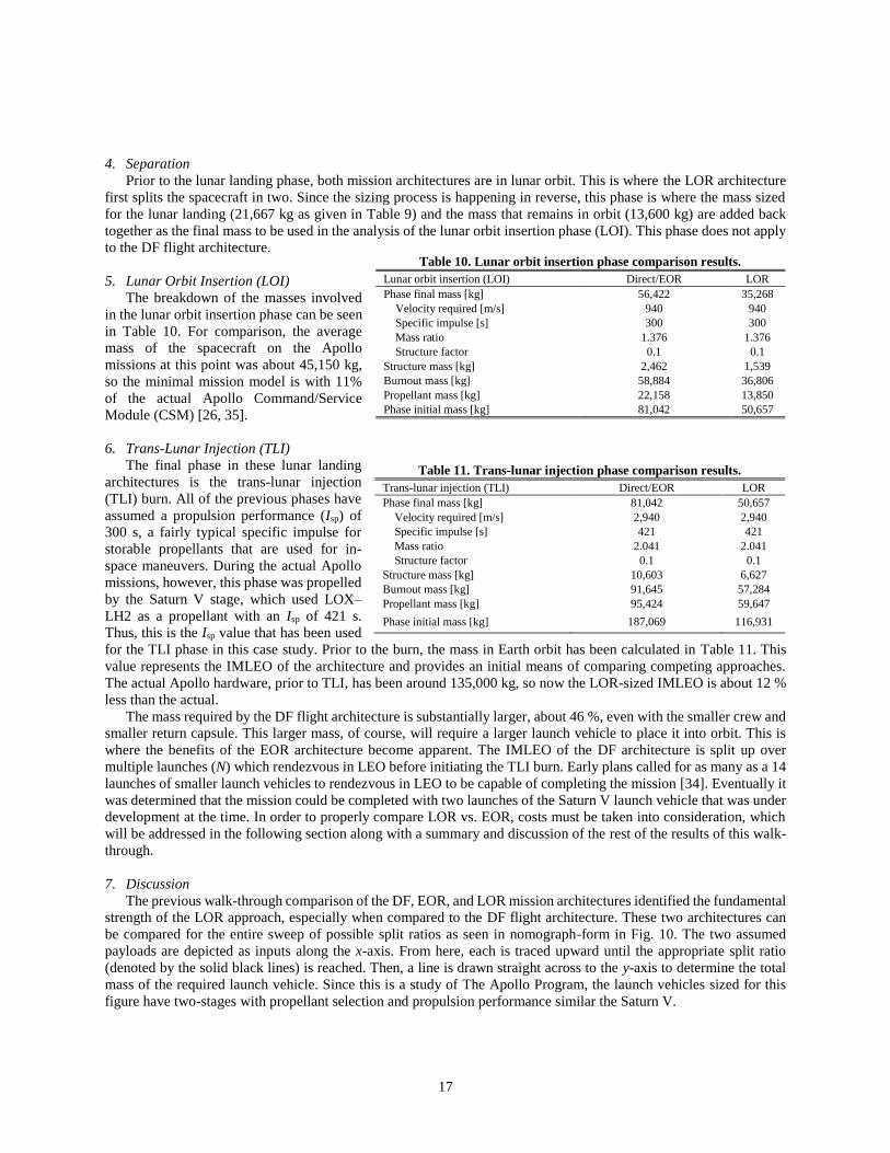
4. Separation

Prior to the lunar landing phase, both mission architectures are in lunar orbit. This is where the LOR architecture

first splits the spacecraft in two. Since the sizing process is happening in reverse, this phase is where the mass sized

for the lunar landing (21,667 kg as given in Table 9) and the mass that remains in orbit (13,600 kg) are added back

together as the final mass to be used in the analysis of the lunar orbit insertion phase (LOI). This phase does not apply

to the DF flight architecture.

5. Lunar Orbit Insertion (LOI)

The breakdown of the masses involved

in the lunar orbit insertion phase can be seen

in Table 10. For comparison, the average

mass of the spacecraft on the Apollo

missions at this point was about 45,150 kg,

so the minimal mission model is with 11%

of the actual Apollo Command/Service

Module (CSM) [26, 35].

6. Trans-Lunar Injection (TLI)

The final phase in these lunar landing

architectures is the trans-lunar injection

(TLI) burn. All of the previous phases have

assumed a propulsion performance (Isp) of

300 s, a fairly typical specific impulse for

storable propellants that are used for in-

space maneuvers. During the actual Apollo

missions, however, this phase was propelled

by the Saturn V stage, which used LOX–

LH2 as a propellant with an Isp of 421 s.

Thus, this is the Isp value that has been used

for the TLI phase in this case study. Prior to the burn, the mass in Earth orbit has been calculated in Table 11. This

value represents the IMLEO of the architecture and provides an initial means of comparing competing approaches.

The actual Apollo hardware, prior to TLI, has been around 135,000 kg, so now the LOR-sized IMLEO is about 12 %

less than the actual.

The mass required by the DF flight architecture is substantially larger, about 46 %, even with the smaller crew and

smaller return capsule. This larger mass, of course, will require a larger launch vehicle to place it into orbit. This is

where the benefits of the EOR architecture become apparent. The IMLEO of the DF architecture is split up over

multiple launches (N) which rendezvous in LEO before initiating the TLI burn. Early plans called for as many as a 14

launches of smaller launch vehicles to rendezvous in LEO to be capable of completing the mission [34]. Eventually it

was determined that the mission could be completed with two launches of the Saturn V launch vehicle that was under

development at the time. In order to properly compare LOR vs. EOR, costs must be taken into consideration, which

will be addressed in the following section along with a summary and discussion of the rest of the results of this walk-

through.

7. Discussion

The previous walk-through comparison of the DF, EOR, and LOR mission architectures identified the fundamental

strength of the LOR approach, especially when compared to the DF flight architecture. These two architectures can

be compared for the entire sweep of possible split ratios as seen in nomograph-form in Fig. 10. The two assumed

payloads are depicted as inputs along the x-axis. From here, each is traced upward until the appropriate split ratio

(denoted by the solid black lines) is reached. Then, a line is drawn straight across to the y-axis to determine the total

mass of the required launch vehicle. Since this is a study of The Apollo Program, the launch vehicles sized for this

figure have two-stages with propellant selection and propulsion performance similar the Saturn V.

Table 10. Lunar orbit insertion phase comparison results.

Lunar orbit insertion (LOI) Direct/EOR LOR


Velocity required [m/s] 940 940








Table 11. Trans-lunar injection phase comparison results.

Trans-lunar injection (TLI) Direct/EOR LOR










18

Figure 10. Validation data on the comparison nomograph of the competing architectures for

manned lunar landing.

The two resulting launch vehicles

are as expected and predicted from

studies during those early years

working on Apollo [11, 36, 37]. The

LOR architecture could be completed

with a launch vehicle similar to the

Saturn V while the DF flight

architecture would likely require a

new class of launcher, like from the

NOVA launch vehicle family. More

important than these two specific

cases, however, is the ability to

observe other possible solutions in the

topography around them.

For example, the gray dashed lines

represent lines of constant mass

returning from the lunar surface.

Assume that an extensive study has

been conducted and determined that

the absolute minimum lunar ascent

module that an organization is

capable of developing for two

astronauts is 2,000 kg. This is close to

the Apollo lunar ascent stage. However, for this hypothetical situation, instead of using a third astronaut in lunar orbit

like Apollo, the mass that remains in orbit is further reduced by remaining unmanned while the two astronauts descend

to the surface. Trace the dashed gray line representing a constant return mass of 2,000 kg down to the left and it can

be seen that as it nears the re-entry mass of the strengthened Gemini capsule, the launch vehicle required is now about

two-thirds the size of the Saturn V. Of course, such an approach would involve a completely new set of risks, but at

least with the visualization of the solution space, the strategic planner is aware of the possibility and can make a better-

informed decision on what needs to be done next.

As previously mentioned, to properly compare EOR with both DF and LOR architectures, the cost of the required

launch vehicles required for the mission must be taken into account. Fortunately, the Ariadne system is capable of

estimating the launch vehicle costs (both development and production). Figure 11 represents the solution space

between all three competing architectures and other combinations of χ and N. The assumed final mission payload mass

in Fig. 11 is the uprated Gemini capsule, 2,500 kg. A sweep of N EOR launches, from 1–3 and a sweep of χ from 0 to

Figure 11. A parametric trade of χ and N for all three mission architectures

competing for The Apollo Program.

19

0.9 created the 15 alternative mission architectures shown in the figure. The final payload is applied to each

architecture and the in-space sizing process applied to determine the IMLEO/N, located along the x-axis. The required

launch vehicle(s) for a given mission are then sized and the total costs estimated, located on the y-axis. To enable

easier comparisons, the total cost has been normalized to the lowest cost architecture. In Fig. 11, this reference

architecture is the one located in the bottom left corner.

This mission architecture involves three

launches to LEO before heading to the

Moon where it uses a split ratio of 0.9,

which is an even higher split than was used

on the Apollo missions. Obviously, such

an architecture would involve additional

hardware complexities and risks that

would have to be evaluated to determine if

the cost savings are worth it or not.

Conversely, the DF flight architecture is

shown in the upper right corner of Fig. 11.

This architecture is the simplest approach

but also the most expensive (around 2.5

times the cost of the reference mission

architecture) and the sheer size of the

launch vehicle required would give rise to

its own unique challenges. Figure 12

includes all three of the competing

architectures with the assumed payloads

used previously in the walk-through of the

phases. The solution space formed by the

solid lines represents the uprated Gemini capsule payload and the dashed lines represent the 6,000 kg Apollo capsule.

Each architecture has been labeled and the required launch vehicle costs can now be consistently compared.

V. Conclusion After discussing the methods used in the Ariadne prototype methodology for launch vehicle sizing, cost estimation,

and mission architecture modeling and sizing, the Ariadne prototype system was applied to The Apollo Program to

validate the methods used and to quantitatively verify that the lunar-orbit-rendezvous mission architecture was the

correct choice for Apollo.

The chosen launch vehicle sizing method, from Chapter V of the Space Planners Guide (SPG), is validated through

a sizing study of the Saturn IB and Saturn V. The SPG estimates the Saturn IB’s total mass to be 15% larger than the

actual total mass, but this is within the stated ±20% accuracy of the SPG, which is sufficient for ruling out less feasible

options. The SPG is then applied to the Saturn V, which results in a -2% error.

After validating the launch vehicle sizing method, the three competing mission architectures, lunar-orbit-

rendezvous (LOR), Earth-orbit-rendezvous (EOR), and direct flight (DF) are modeled with a focus on two key

parameters, the split ratio and the number of launches. By specifying these two parameters, the in-space elements for

each mission architecture are sized using the prototype sizing methods. Once the initial mass in low Earth orbit for

each of the three competing architectures are known, a launch vehicle could be sized for each mission architecture.

Then, using the two parameters, a solution space of launch vehicle total mass to Earth return mass is generated that

shows how the LOR mission architecture enables a significantly lower launch mass compared to direct flight (DF).

Using the cost estimation methods, a subsequent solution space of launch vehicle cost to mass to LEO per launch

shows that the LOR mission architecture is significantly less expensive than the EOR mission architecture.

These two solution spaces quantitatively reveal that the Apollo LOR mission architecture was indeed the correct

selection when compared to the EOR and DF mission architectures. Later investigations into The Apollo Program will

explore the effects of the mission architecture selection on the entire program and compare alternative program

objectives with the historical objectives of Apollo.

Figure 12. Validation data on the solution space of the three competing

mission architectures for The Apollo Program.

20

Appendix

Figure A.1. Staging and specific impulse effects on payload performance (V.C-9) [14].

Figure A.2. Launch vehicle maximum dimensions (V.C-10) [14].

Figure A.3. Stage to payload mass ratios (V.C-11) [14].

21

Figure A.4. Stage to payload mass ratio conversion to stage mass ratio (V.C-12) [14].

Figure A.5. Liquid first stage structure factor (V.C-15) [14].

Figure A.6. Liquid second stage structure factor (V.C-16) [14].

22

Figure A.7. Optimum launch vehicle sizing nomograph (V.C-22) [14].

Figure A.8. Stage velocity versus mass ratio and specific impulse (V.C-23) [14].

23

Figure A.9. Stage mass ratio vs stage mass ratio (V.C-24) [14].

24

References [1] Kennedy, J. F. "Special Message To The Congress On Urgent National Needs." online: G. Peters and J.T. Wolley, The

American Presidency Project [accessed March 2016], http://www.presidency.ucsb.edu/ws/?pid=8151, 1961.

[2] Coley Jr., M. D., Maynard, I. W., Seyed Alavi, K., and Chudoba, B. "Ariadne: A Space Program Forecasting and Planning

Decision Support Tool for Strategic Planners," Space and Astronautics Forum and Exposition. American Institute of

Aeronautics and Astronautics, Orlando, Florida, 2018.

[3] Coley Jr. , M. D. "On Space Program Planning: Quantifying the Effects of Spacefaring Goals and Strategies on the Solution

Space of Feasible Programs." The University of Texas at Arlington, 2017.

[4] Twiss, B. C. Forecasting for Technologists and Engineers: A Practical Guide for Better Decisions: London, United Kingdom:

Peter Peregrinus, 1992.

[5] Coley Jr., M. D., Maynard, I. W., Seyed Alavi, K., and Chudoba, B. "Space Mission Architecture Synthesis: The Need for a

Top-Down Program Planning Approach," Space and Astronautics Forum and Exposition. American Institute of

Aeronautics and Astronautics, Orlando, Florida, 2018.

[6] Astronautics, G. D. "STAMP - Space Technology Analysis and Mission Planning - Volume III - General Report." General

Dynamics, 1965.

[7] Sutton, G. P., and Biblarz, O. Rocket Propulsion Elements: John Wiley \& Sons, Inc., 2010.

[8] Blasingame, B. P., and Brown, K. Space Logistics Engineering: Wiley, 1962.

[9] Wertz, J. R., Everett, D. F., and Puschell, J. J. Space Mission Engineering: the New SMAD: Hawthorne, CA: Microcosm Press,

2011.

[10] Mickelwait, A. B. "Lunar Missions: Launch to Rendezvous," Technology of Lunar Exploration. Vol. 10, Academic Press,

1962, pp. 139-165.

[11] Amster, W. H. "Launch Vehicle Peformance," Technology of Lunar Exploration. Vol. 10, Academic Press, 1962, pp. 167-

182.

[12] Houbolt, J. C. "Manned Lunar-landing Through use of Lunar-orbit Rendezvous." Langley Research Center: NASA, 1961.

[13] Hammond, W. E. Design Methodologies for Space Transportation Systems: Reston, VA: American Institute of Aeronautics

and Astronautics, 2001.

[14] Harney, E. D. Space Planners Guide: Air Force Systems Command, US Air Force, 1965.

[15] Koelle, D. E. Handbook of Cost Engineering and Design of Space Transportation Systems: TCS - TransCostSystems, 2016.

[16] Anon. "Report of the Horizontal Launch Study - Interim Report." NASA/DARPA, 2011.

[17] Bartolotta, P. A., Buchen, E., Engelund, W. C., and others. "Horizontal Launch: a Versatile Concept for Assured Space Access

- Report of the NASA-DARPA Horizontal Launch Study." NASA/DARPA, 2011.

[18] Sforza, P. M. Manned Spacecraft Design Principles: Elsevier, Inc., 2015.

[19] Akens, D. S. "Saturn Illustrated Chronology - Saturn's First Eleven Years." NASA - Marshall Space Flight Center, 1971.

[20] Anon. "Manned Lunar Landing Program Mode Comparison." NASA, 1962.

[21] Allday, J. Apollo in Perspective: Spaceflight Then and Now: CRC Press, 1999.

[22] Koelle, H. H., and Thomae, H. F. "Mission Velocity Requirements And Vehicle Characteristics," Handbook of Astronautical

Engineering. McGraw-Hill Book Company, Inc, 1961, pp. 14-48.

[23] Jones, R. M. "Integrated Space Plan." Poster, version 4.0, 1997.

[24] Analytics, I. S. "Integrated Space Plan." Poster, 2015.

[25] 111th Congress. "NASA Authorization Act of 2010." Public Law 111-267, 2010.

[26] Orloff, R. W. Apollo by the Numbers: A Statistical Reference: New York: Springer-Verlag, 1996.

[27] Ezell, L. N. NASA Historical Data Book - Volume II: NASA, 1988.

[28] Anon. "Technical Information Summary - Apollo 11 (AS-506) - Apollo Saturn V Space Vehicle." NASA - George C. Marshall

Space Flight Center, 1969.

[29] Lawrie, A., and Godwin, R. Saturn V: The Complete Manufacturing and Test Records: Plus Supplemental Material: Apogee,

2005.

[30] NASA. "Lunar Orbit Rendezvous." News Conference on Apollo Plans at NASA Headquarters, 1962.

[31] Brooks, C. G., and Ertel, I. D. The Apollo Spacecraft - A Chronology - Volume III: NASA, 1976.

[32] Logsdon, J. M. "Selecting the Way to the Moon: the Choice of the Lunar Orbital Rendezvous Mode," Aerospace Historian

Vol. 18, 1965, pp. 63-70.

[33] Hansen, J. R. "Enchanted Rendezvous - John C. Houbolt and the Genesis of the Lunar-Orbit Rendezvous Concept."

Washington, DC: NASA, 1999.

[34] Logsdon, J. M. "NASA's Implementation of the Lunar Landing Decision." The Catholic University of America, 1969.

[35] Orloff, R. W., and Harland, D. M. Apollo: The Definitive Sourcebook: Springer Science & Business Media, 2006.

[36] Gilruth, R. R., and Faget, M. A. "The Manned Lunar Mission," American Rocket Society - Lunar Missions Meeting. 1962.

[37] Logsdon, T. Orbital Mechanics: Theory And Applications: New York: John Wiley & Sons, 1998.

http://www.presidency.ucsb.edu/ws/?pid=8151

A Parametric Case Study of the Apollo Program: Launch ...

Documents

Transcript of A Parametric Case Study of the Apollo Program: Launch ...