A NUMERICAL ANALYSIS FOR THE BENDING OF...

AN IMPROVED BENDING MODEL FOR THERMOPLASTIC COMPOSITES IN FORMING PROCESSES BY M. S. VOORMOLEN

1

ABSTRACT

The purpose of this research is to elaborate a mathematical model that describes the visco-

elastic bending behavior of a thermoplastic composite specimen during thermoforming

processes. The mathematical model was derived from a simplified physical model which

represents a layered composite material of alternating elastic and viscous layers. In a previous

research the viscous layers are assumed to be from Newtonian fluid, having a constant shear

viscosity, while the elastic layers are linear elastic. This resulted in a mathematical model in form

of the diffusion equation, describing a diffusive-like behavior of the deflection angles in the beam.

Because polymeric melts exhibit in general a shear thinning behavior, the diffusion equation in

this research is improved by including the shear rate dependency of the melt viscosity.

Therefore, the diffusion equation became a non-linear differential equation, which is solved

numerically by means of the finite difference method. This research shows the significance of the

shear thinning behavior in the model by comparing the bending deformation of the composite

beam obtained with a constant viscosity and a shear-thinning viscosity.


2

ACKNOWLEDGEMENTS

This is the report of the bachelor assignment from Advanced Technology. This research is done

at the research group Production Technology in the department of Mechanical Engineering at the

University of Twente and in cooperation with the ThermoPlastic composite Research Centre

(TPRC).

I would like to thank Remko Akkerman for helping me find this assignment and introducing me to

thermoplastic composites. The challenging discussions and the good feedback has helped me a

lot in the understanding of the problem and the context around it. I also would like to give a great

thanks to Ulrich Sachs, we had a great cooperation and you were always there when I needed

help. Your readiness to help me out and send me in the right direction where a great help.


3

TABLE OF CONTENTS

1 Introduction 4

2 Theoretical background 5 2.1 Thermoplastic composites 5 2.2 Bending in forming processes 5 2.3 Bending experiment 6 2.4 Bending model 6 2.5 Assumptions for the mathematical model 7 2.6 Deriving the mathematical model 8 2.7 Boundary conditions 10 2.8 Solution mathematical model 10 2.9 Non-Newtonian fluids 11

3 Method 14 3.1 Finite Difference Method 14 3.1.1 The explicit method 15 3.1.2 The implicit method 15 3.2 Defining parameters with a variable viscosity 16 3.3 Solving method 16 3.4 Validation of the numerical model 17

4 Results 18 4.1 The local deflection angle 18 4.2 Diffusion coefficient 20 4.3 Shear stress and force 21

5 Discussion 23 5.1 Comparison to the old model 23 5.2 Comparison to experimental results 23 5.3 The effect of thickness and temperature 24 5.4 Assumption check 24

6 Conclusion and recommendations 26

7 Appendix 27 7.1 Summation of variables 27 7.2 Matlab script 28

8 References 28


4

1 INTRODUCTION

Climate change has become over the years a popular subject. People are nowadays more aware

of the consequences of our current life style. Creating an ecofriendly society has become a more

important item on the agenda for more governments. In June 2015, the Dutch government has

received the verdict that it has to reduce the greenhouse gas CO2 with 25% in 2020 [1].

At the same time, society is not willing to pay huge amounts extra or reduce their luxury in order

to help this cause. This creates a large challenge and has caused researchers to search for

alternatives, which are cheap, can provide luxury and lower emissions.

The ThermoPlastic composite Research Center (TPRC) is one of the places where researchers

are doing research into a new material. This material, thermoplastic composites, can replace the

current building materials in the automotive and aerospace industry. It is a lighter alternative and

lighter vehicles have a lower emission rate. As an added bonus, thermoplastic composites also

form a tougher and stronger material [2].

At this moment, the thermoset composites are often used even though thermoplastic composites

have a higher toughness and impact damage resistance [2]. The reason for this is that thermoset

composites have lower material costs [3]. However they are less suitable for automated

processes and the products are mainly made by hand lay-up. Thermoplastic composite are more

suitable for production processes, because of the melting property of thermoplastics. However

the behavior of thermoplastic composites in a forming process is complicated. Currently there is

a lag in knowledge about their behavior, which prevents the material from becoming popular in

use. [3]

When this knowledge gap has been bridged, the thermoplastic composites will play a larger role

in the automotive and aerospace industry. Apart from being tougher and less prone to damage,

thermoplastic composites also have the property of being recyclable. Production will be a lot

cheaper as well, due to the fact that thermoplastics are easier to handle in forming processes.

Currently the TPRC, together with BOEING, Fokker, Ten Cate and the University of Twente, is

doing research to close the knowledge gap in the behavior of this material. This is done by

predicting the behavior of the thermoplastic composites in different production operations.

In this paper the bending of a thermoplastic composite will be discussed. By predicting the

behavior of the composite during the bending process, the reluctance of the material to bend can

be determined. With this information, the bending process can be optimized to prevent formability

problems.

Currently there is a model on the behavior of the composite during the bending process.

This model is however very simplified. In this report the model will be elaborated.


5

2 THEORETICAL BACKGROUND

2.1 Thermoplastic composites

In order to predict the bending behavior, the structure of a thermoplastic composites is essential.

A composite material is a material that consists of a stack of multiple materials. These materials

keep their own material properties, but put together other characteristics appear. In the case of

thermoplastic composites, it is a stack of alternating layers of fiber (e.g. glass fiber) and

thermoplastic polymers. The fiber layer can have a woven structure of polymers or a

unidirectional (UD) structure, see figure 1. UD composites are for production and stiffness

reasons more beneficial, however it does cause more problems when bending the material [2].

This research considers the UD fiber reinforced polymers in the thermoplastic layer of the

composite.

FIGURE 1: UNIDIRECTION COMPOSITES [5]

Thermoplastics, also known as thermosoftening plastics, are a type of material that consists of

long polymer chains (figure 2). Thermosoftening plastics melt when temperature is increased and

harden out when the temperature is lowered again. This explains why this material is easy to

produce and is suited very well for recycling

FIGURE 2: POLYETHERETHERKETONE (PEEK) [6]

2.2 Bending in forming processes

In the bending process, the material must not lose any of its strength and toughness. This is

prevented by heating the composite above melting temperature of the thermoplastic during the

bending process. When the bending process is completed, the specimen is cooled down. This

process prevents the composite from having to bend in the solid phase, which would cause

stress on the polymers. Instead the polymer layer is able to form in the molten phase, resulting in

having the same toughness as before can be achieved if it is well consolidated.


6

2.3 Bending experiment

The bending of a thermoplastic composite is done with the use of a rheometer. The rheometer

has a thermal chamber which will heat up the specimen above melting temperature. When the

chamber is at the right temperature, the specimen will be clamped in the two fixtures as can be

seen in figure 3. One fixture stays at a zero degree angle (the reference angle) and the second

fixture will rotate around the shaft at a constant velocity (ω).

To rotate and therefore bend the specimen, a certain amount of moment (Mc) has to be exerted

by the rotating shaft. This moment is dependent on the amount of resisitance the specimen has

to bend. The rheometer can measure the moment exerted on the shaft and thus measuring the

reluctance of the specimen to bend.

FIGURE 3: RHEOMETER USED IN RESEARCH U. SACHS [2]

2.4 Bending model

To predict the behavior of the specimen during the experiment a model is made. In order to make

a feasible model the following simplifications are made:

- The fibers and matrix are evenly distributed. - The fibers and matrix are modeled as layers with a homogeneous thickness, ℎ𝑓 and

ℎ𝑚, respectively.

Now that the model is simplified, the forces and moments can be considered.

The specimen will bend due to the moment 𝑀 put upon the end. This moment will only bend the

fiber layers - the matrix layers cannot carry moments, due to their melted phase. The fiber layer

will also experience a transverse force 𝑉 and a normal force 𝑁 as a result of the fixtures.

Due to the fact that the laminate is a stack of fiber layers (alternated with matrix layers), the

separate layers bend separate of each other. As a result they slide relative to each other, figure

4. This sliding will result in a relative shear force. A shear force is a force that in the direction of

the slide, it will try to deform the material it is being exerted on. The shear force caused by the

sliding of the fiber layers is related to the height of the matrix layer and the size of the step looked

into. This has to do with the viscosity of the matrix layer, if the layer is really thin the shear force

should be larger to make the deformation (by sliding the fiber layer). The force is also linear to


7

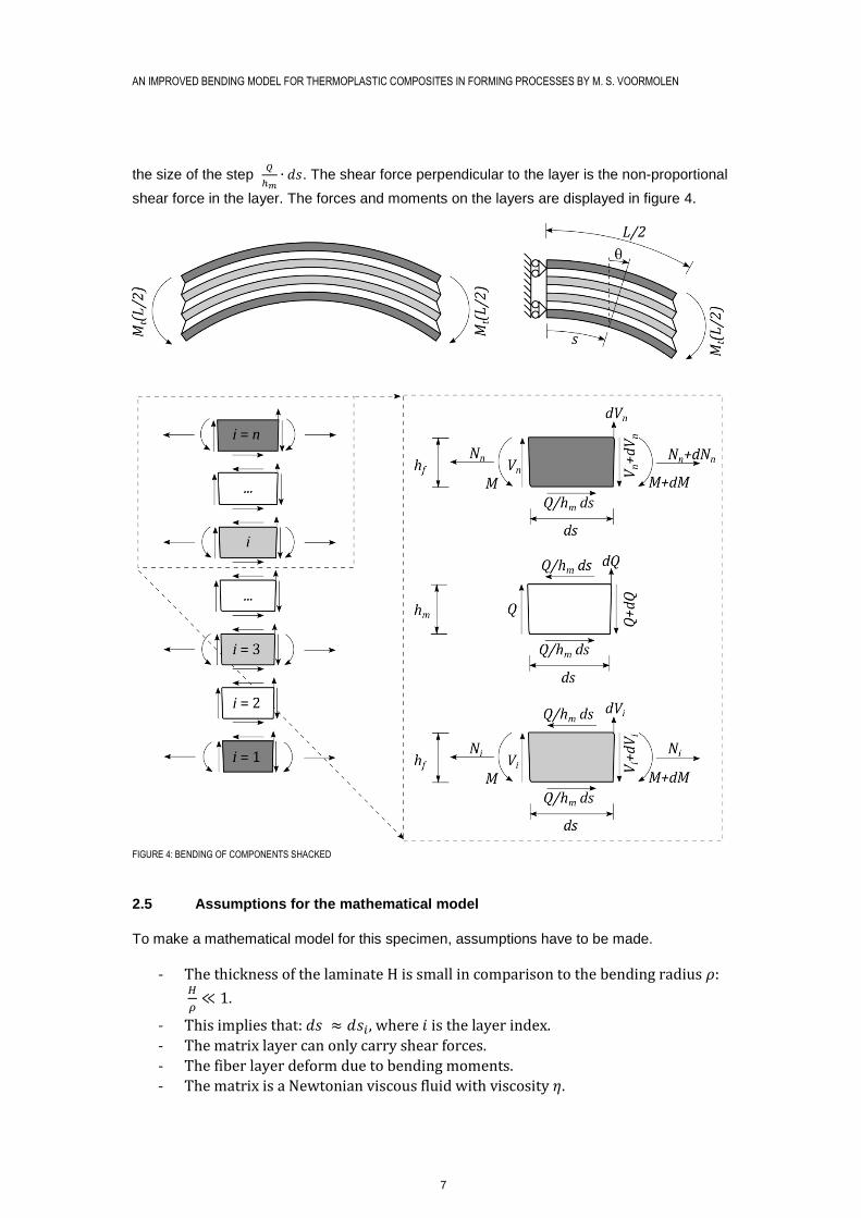
the size of the step 𝑄

ℎ𝑚∙ 𝑑𝑠. The shear force perpendicular to the layer is the non-proportional

shear force in the layer. The forces and moments on the layers are displayed in figure 4.

FIGURE 4: BENDING OF COMPONENTS SHACKED

2.5 Assumptions for the mathematical model

To make a mathematical model for this specimen, assumptions have to be made.

- The thickness of the laminate H is small in comparison to the bending radius 𝜌:

𝐻

𝜌≪ 1.

- This implies that: 𝑑𝑠 ≈ 𝑑𝑠𝑖, where 𝑖 is the layer index.

- The matrix layer can only carry shear forces.

- The fiber layer deform due to bending moments.

- The matrix is a Newtonian viscous fluid with viscosity 𝜂.


8

- The fiber is a Hookian elastic solid with elastic modulus 𝐸.

- The deformation of the laminate is considered small. Thus neglecting non-linearity by deformation.

- All fiber layers deform equally: 𝑀 = 𝑀𝑖 and 𝑑𝑀 = 𝑑𝑀𝑖, ∀𝑖. - All matrix layers deform equally: 𝑄 = 𝑄𝑖 and 𝑑𝑄 = 𝑑𝑄𝑖 , ∀𝑖.

2.6 Deriving the mathematical model

To derive the mathematical model, the magnitude of the shear force has to be defined. In the

work of Sachs the definition was formed for the shear 𝛾 of a thermoplastic composite as a

function of the deflection angle 𝜃 [2]. This relation is based on the fundaments of the azimuthal strain (strain in a bending situation) of a single layer. Since ℎ𝑓 and ℎ𝑚 are independent on time,

the time derivative of shear, the shear rate �̇�, is therefore in the same way related to the rate of

deflection angle �̇�.

𝛾 = (ℎ𝑓

ℎ𝑚

+ 1) 𝜃 1.

This relation is combined with the definition of the shear force with 𝑊 as the width of the specimen. Since ℎ𝑓 and ℎ𝑚 are independent on time, the time differentiable of shear, the shear

rate, is therefore in the same way related to the rate of deflection angle.

𝑄 = 𝜂𝜕𝛾

𝜕𝑡ℎ𝑚𝑊 = 𝜂 (

ℎ𝑓

ℎ𝑚

+ 1) �̇� ℎ𝑚𝑊 2.

Now that the shear force is defined, the moment equilibrium has to be determined for a fiber unit cell embedded by matrix, 𝑖𝑛 ∈ {3, 5, 7,… , 𝑛 − 2}:

𝑑𝑀 + 𝑉𝑖𝑛 𝑑𝑠 − 𝑄ℎ𝑓

ℎ𝑚𝑑𝑠 = 0. 3.

The moment equilibrium for a fiber unit cell on the outer surface, 𝑜𝑢𝑡 ∈ {1, 𝑛}:

𝑑𝑀 + 𝑉𝑜𝑢𝑡 𝑑𝑠 − 𝑄1

2

ℎ𝑓

ℎ𝑚𝑑𝑠 = 0.

4.

By subtracting equation 4 from equation 3 the following relation between the transverse forces

and the shear force is determined.

𝑉𝑖𝑛 = 𝑉𝑜𝑢𝑡 + 𝑄1

2

ℎ𝑓

ℎ𝑚. 5.

A force equilibrium considering all n layers yields:

𝑛 − 3

2 𝑑𝑉𝑖𝑛 + 2𝑑𝑉𝑜𝑢𝑡 = −

𝑛 − 1

2𝑑𝑄. 6.


9

Equation 6 is integrated from 𝑠 = 0 till 𝑠 = 𝐿. Since the shear force and the transverse force are

zero at 𝑠 = 0, forces are considered at 𝑠 = 𝐿 and the equation simplifies:

𝑛 − 3

2 𝑉𝑖𝑛 + 2𝑉𝑜𝑢𝑡 = −

𝑛 − 1

2𝑄. 7.

Solving with equation 5 for 𝑉𝑜𝑢𝑡:

𝑉𝑜𝑢𝑡 = −(𝑛 − 1

𝑛 + 1+

1

2

𝑛 − 3

𝑛 + 1

ℎ𝑓

ℎ𝑚)𝑄 8.

Assuming 𝑛 ≫ 1:

𝑉𝑜𝑢𝑡 ≈ −(1 +1

2

ℎ𝑓

ℎ𝑚)𝑄 9.

Solving for 𝑉𝑖𝑛:

𝑉𝑖𝑛 = −(𝑛 − 1

𝑛 + 1−

ℎ𝑓

ℎ𝑚

2

𝑛 + 1)𝑄 10.

Assuming 𝑛 ≫ 1:

𝑉𝑖𝑛 = −𝑄 11.

The final differential equation is based on the moment equilibrium of a fiber unit cell embedded

in the matrix:

𝑑𝑀 + 𝑉𝑖𝑛 𝑑𝑠 − 𝑄ℎ𝑓

ℎ𝑚𝑑𝑠 = 0 12.

𝜕𝑀

𝜕𝑠− (1 +

ℎ𝑓

ℎ𝑚)𝑄 = 0 13.

The moment in the fiber is related to its curvature according to the Euler-Bernoulli beam

theorem, with 𝐼 as the second moment of area of the fiber layer:

𝑀 =𝜕𝜃

𝜕𝑠𝐸𝐼. 14.

Substitution of 𝑀 and 𝑄 by the constitutive equations, will result in a partial differential,

diffusion, equation.

𝐷𝜕2𝜃

𝜕𝑠2−

𝜕𝜃

𝜕𝑡= 0 15.

𝐷 =𝐸𝐼𝑓

𝜂(1 +ℎ𝑓

ℎ𝑚) (ℎ𝑓 + ℎ𝑚)𝑊

16.


10

2.7 Boundary conditions

In order to solve the partial differential equation, boundary conditions are necessary. Boundary

conditions describe the deflections already known. In this set of equations there are three

different boundary conditions given, in which N represent the amount of space steps, ω the

angular velocity of the fixture and ∆𝑡 the size of the time step.

1. At time 𝑗 = 0, the specimen is flat: 𝜃𝑖,0 = 0 ∀ 𝑖.

2. At space step 𝑖 = 1, the specimen will not deflect: 𝜃1,𝑗 = 0 ∀ 𝑗.

3. At space step 𝑖 = 𝑁, the specimen has the same angle of the fixture:

𝜃𝑁,𝑗(𝑗) =𝜔

2∙ 𝑗 ∙ ∆𝑡 ∀ 𝑗. With 𝜔 as the angular velocity of the fixture.

2.8 Solution mathematical model

In figure 5 the solution of this diffusion equation is displayed, considering a specimen with a

length of 7.5 mm, an angular velocity of the fixure 𝜔 =𝜋

3 and a diffusion coefficient 𝐷 = 7.7908 ∙

10−7.

FIGURE 5: THE SOLUTION OF THE DIFFUSION EQUATION WITH A CONSTANT VISCOSITY OF 7.7908E-7

Equation 15 can be recognized as the diffusion equation in which 𝐷 represents the diffusion

coefficient or diffusivity. The diffusion coefficient indicates the rate of the diffusion. In this case

the diffusion coefficient is dependent on the bending stiffness, the width of the specimen and the

height of both the fiber layer and the matrix layer.

When the diffusion coefficient is infinite the local deflection angle moves instantly and linear

throughout the whole specimen. At a diffusion coefficient approaching zero (e.g. 1 ∙ 10−15), the

specimen is very reluctant to the given angle, and will stay straight as long as possible. The final

deflection angle along the specimen for different values of the diffusion coefficient can be seen in

figure 6.


11

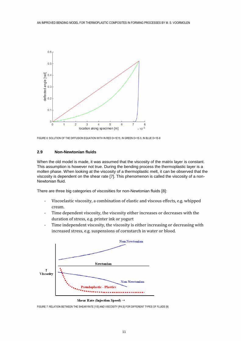
FIGURE 6: SOLUTION OF THE DIFFUSION EQUATION WITH IN RED D=1E15, IN GREEN D=1E-5, IN BLUE D=1E-8

2.9 Non-Newtonian fluids

When the old model is made, it was assumed that the viscosity of the matrix layer is constant.

This assumption is however not true. During the bending process the thermoplastic layer is a

molten phase. When looking at the viscosity of a thermoplastic melt, it can be observed that the

viscosity is dependent on the shear rate [7]. This phenomenon is called the viscosity of a non-

Newtonian fluid.

There are three big categories of viscosities for non-Newtonian fluids [8]:

- Viscoelastic viscosity, a combination of elastic and viscous effects, e.g. whipped

cream.

- Time dependent viscosity, the viscosity either increases or decreases with the

duration of stress, e.g. printer ink or yogurt

- Time independent viscosity, the viscosity is either increasing or decreasing with

increased stress, e.g. suspensions of cornstarch in water or blood.

FIGURE 7: RELATION BETWEEN THE SHEAR RATE [1/S] AND VISCOSITY [PA.S] FOR DIFFERENT TYPES OF FLUIDS [9]


12

Thermoplastics often exhibit a shear thinning behavior, which decreases with an increasing

shear rate. Shear rate is the rate at which a progressive shearing deformation is applied to the

material [10]. Since the diffusion coefficient is inversely proportional to the viscosity, the diffusion

coefficient increases when the shear rate increases.

The shear rate dependent viscosity for UD carbon PEEK was investigated by several researches

done by different institutes, including the University of Twente [2] [11] [12]. When displayed in a

logarithmic graph a clear relation between the viscosity and the shear rate can be seen in figure

7.

𝜂 = 𝐾 �̇�𝑚 17.

The constants however are not exactly the same for the different experiments even though the

same polymer is used. This difference can be explained by the different temperatures at which

the experiments are done or the different grade of polymer used [7]. But it is very likely, that the

measuring methods are different for each researcher. Therefore only speculation can be made

from this data. These speculations have to be tested experimentally by using the same

measuring methods with different conditions.

FIGURE 8: RELATION VISCOSITY AND SHEAR STRESS. × SACHS ET AL (UD CARBON PEEK AT 385°C); □ STANLEY AND MALLON (APC-2 AT 380°C); ◊

SACHS ET AL. (UD CARBON PEEK AT 390°C); Δ GROVES (UD CARBON PEEK AT °C) [2]

With the relation between the viscosity and the shear rate, the diffusion equation can be updated.

The diffusion coefficient is dependent on the shear rate.

This result can also be verified with the measurements of the exerted moment on the shaft during

the bending process. If the relation was purely visco-elastic, there would be a linear relation

between the moment and the angle. As can be seen in figure 9, the relation is not linear. At low

angles the moment is small, then the relation between the rotation angle and the moment are

almost linear, up to the point when the angle is above approximately 50º.

In figure 9, the moment is measured at different angular velocities (�̇�). A higher velocity would

logically cause a higher shear rate, thus resulting in different values for the viscosity and the

diffusion coefficient [2].


13

FIGURE 9: THE MOMENT THAT IS EXERTED ON THE SHAFT VS THE ANGLE OF THE BENDING FIXTURE, THE DOTT\

ED LINES REPRESENT THE FITTED MODEL OF SACHS.


14

3 METHOD

3.1 Finite Difference Method

When solving non-linear differential equations, like the diffusion equation with a shear rate

dependent diffusion coefficient, an analytical approach is not always possible. Therefore the

equation is solved numerically by using the finite difference method.

In this method the differential equations are converted into difference equations. These

difference equations give an approximate of the first and second derivative at numerous points of

interest. When this is done with infinitively many points an exact solution is established. However

this is not possible and a finite number of points can give a fairly good solution as well. The

amount of steps is inversely proportional to the step size. When the step size is small relative to

the distance, the finite difference method gives a good estimate.

The two equations below represent the ways in which a first derivative and a second derivative

are translated to the finite difference method. In this case the diffusion equation is being solved.

The diffusion equation (equation 15) has the property that it contains the first derivative of time

and the second derivative in space. 𝑖 is the index of the space step and 𝑗 is the index of the time

step. ∆𝑠 and ∆𝑡 represent respectively the size of the space step and the size of the time step.

𝐷 𝜃𝑖+1,𝑗 − 2𝜃𝑖,𝑗 + 𝜃𝑖−1,𝑗

∆𝑠2−

𝜃𝑖,𝑗+1 − 𝜃𝑖,𝑗−1

2∆𝑡≈ 0 18.

In this equation data are used both from a previous time step and one in the future, which gives

complications when solving diffusion equations. Therefore a slightly less accurate translations

must be used, considering only 2 different time steps.

𝜕𝜃

𝜕𝑡=

𝜃𝑖,𝑗+1 − 𝜃𝑖,𝑗

∆𝑡 19.

When implementing this into the diffusion equation, there are two options. Taking the second

derivative in time 𝑗 or in time 𝑗 + 1.Both ask for a different solving method, respectively the

explicit method and the implicit method. Both methods are displayed in a stencil in figure 10.

This method can be explained with the use of a stencil representing the two. The deflections at

time 𝑗 are known, the deflections at 𝑗 + 1 are asked.

FIGURE 10: STENCIL REPRESENTING A) THE EXPLICIT METHOD AND B) THE IMPLICIT METHOD


15

Both methods are equally capable in solving the regular diffusion equation. Both will be

elaborated on in the following paragraphs.

3.1.1 The explicit method

The explicit method calculates with the use of three different points, one point in the next time

step. Mathematically it looks like this.

𝜃𝑖,𝑗+1 =𝐷 ∙ ∆𝑡

∆𝑠2 (𝜃𝑖+1,𝑗 − 2𝜃𝑖,𝑗 + 𝜃𝑖−1,𝑗) + 𝜃𝑖,𝑗 21.

The first term of this expression is also known as the Fourier number. This number is crucial for

solving the equation.

𝐹 =𝐷 ∙ ∆𝑡

∆𝑠2≤ 0.5 22.

For having a stable reliable solution, the Fourier number should be lower or equal to 0.5.

Translated to the physical relation this means that the beam will bend the right way. When the

Fourier number exceeds 0.5, the specimen will bend according to the red line in figure 11.This

shape does not makes sense in physical context and it will result in an unstable result.

FIGURE 11: PHYSICAL EXPLANATION OF THE FOURIER NUMBER

The Fourier number is dependent on the size of the time step, space step and of the diffusion

coefficient. In regular cases this condition is within reach, which makes it a favorable approach,

because it is numerically stable and also less intensive for large calculations [13]. In most cases

this is a good choice for the calculations. However in this case, the Fourier number becomes too

complicated to find a suitable space and time step size.

3.1.2 The implicit method

The implicit method is a more numerical intensive solving method. Instead of a direct equation for

a next point, this method is based on matrix calculations. These matrix calculations are based on

the mathematical principle that a set of equations can be solved, if the amount of equations is

equal to the amount of unknowns.

In this method the equation will be separated in a matrix with variables and two vectors, one

containing the unknown angles of the current time step, one containing the boundary conditions

and information about the previous time step.

−𝐷 ∙ ∆𝑡

∆𝑠2 𝜃𝑖+1,𝑗+1 + (

2 ∙ 𝐷 ∙ ∆𝑡

∆𝑠2+ 1) ∙ 𝜃𝑖,𝑗+1 −

𝐷 ∙ ∆𝑡

∆𝑠2 𝜃𝑖−1,𝑗+1 = 𝜃𝑖,𝑗 23.


16

[

1 0 0−𝐹 1 + 2 ∙ 𝐹 −𝐹0 −𝐹 1 + 2 ∙ 𝐹

0 0 0 0 0 0

−𝐹 0 0 0 0 −𝐹 0 0 0 0 0 0

1 + 2 ∙ 𝐹 −𝐹 0−𝐹 1 + 2 ∙ 𝐹 −𝐹0 0 1 ]

∙

[

𝜃1,𝑗

𝜃2,𝑗

⋮⋮

𝜃𝑁−1,𝑗

𝜃𝑁,𝑗 ]

=

[

0𝜃2,𝑗−1

⋮⋮

𝜃𝑁−1,𝑗−1

𝜔

2∗ 𝑗 ∗ ∆𝑡]

24.

The matrix and the vector on the right hand side are known, therefore the local deflection angles

can be calculated. This method has been proved, suitable for a variable diffusion coefficient.

3.2 Defining parameters with a variable viscosity

The diffusion coefficient is defined as a function of the viscosity. As seen in the previous chapter

the viscosity is not constant, but a function of the shear rate (equation 17).

Looking into the literature, this relation describes the power-law of fluid, also known as the

Ostwald-de-Waele relationship.

𝜏 = 𝐾 �̇�𝑛 = 𝜂 �̇� ⇒ 𝜂 = 𝐾 �̇�𝑛−1 ⇒ 𝑚 = 𝑛 − 1 25.

The relation between the shear rate and the rate of the deflection angle, is described in equation

1.

When these relations are substituted in the diffusion coefficient, the diffusion coefficient has

become a function of the rate of deflection angle.

𝐷 = 𝐸𝐼𝑓

𝑊(ℎ𝑓 + ℎ𝑚) (1 +ℎ𝑓

ℎ𝑚)1+𝑚

𝐾�̇�𝑚

26.

3.3 Solving method

Due to the shear rate dependency of the diffusion coefficient, its value becomes also unknown

and has to be solved for each position in each time step. In order to find the diffusion coefficient

for each time step an iterative scheme is applied, shown in figure 12.

FIGURE 12: ITERATION SCHEME

With the use of a guessed diffusion coefficient the matrix (equation 24) is filled. The right hand

side is filled with the first boundary conditions at 𝑗 = 0. Using the inverse matrix equation the

new deflection angles are calculated. With the deflections at the previous time step the angular

velocity of deflection is calculated for each space step, as well as the shear rate, the viscosity

D(i,j)

u(i,j)

�̇�𝜂

D(i,j)


17

and the new diffusion coefficients. These coefficients are compared to the guessed ones and the

error between the two is calculated. When the error is too large the calculations are done again,

instead of guessing, this time the new diffusion coefficients will be placed in the matrix. The

deflection angles are recalculated and the process as shown in figure 12, starts again. This cycle

will be repeated until the largest error of the space steps is small enough. When this is achieved,

a new time step will be calculated. The boundary conditions at the right hand side are replaced

by the angles of the previous time step.

In order to prevent the loop continuing on infinitely, the error is set at 1 ∙ 10−10 𝑚2

𝑠, approximately

0,01% of the first guessed diffusion coefficient.

A problem with this method occurs when there is no shear. This makes the matrix in equation 24

singular and therefore it cannot be solved. To prevent this a minimum of 1 ∙ 10−15 is applied.

Every diffusion coefficient below this minimum will be defined at this minimum. Apart from this

minimum there is also a maximum amount of iterations given. This prevents the script from

getting stuck in a loop.

3.4 Validation of the numerical model

To check if the results are valid three different actions are taken.

First the result will be checked for the situation where the diffusion coefficient is known. The

diffusion coefficient must be zero around 𝑠 = 0 for the first time steps. The diffusion coefficient

also ends at a prescribed value, as the angular velocity of the shaft is known. When this is

correct, it can be stated that the matlab script does not contain errors with the boundary

conditions.

The second validation step is by increasing the number of time steps and space steps. According

to the finite difference method, when the amount of steps becomes infinite the results will be

exact. Thus by increasing the steps the results become more accurate. However the basic shape

should not differ that much between 200 and infinity. When this is correct, it can be stated that

the solution is converging if the discretization steps are made smaller.

The last step will consist of increasing the iteration steps. According to the iteration method, if

infinitely many steps are made the right answer will be found in theory, but it can also become

stuck in a loop. To validate the results the amount of iterations can be increased, this could not

affect the basic shape of the result. With this method a suitable amount of iterations can be

chosen to run the script on.


18

4 RESULTS

4.1 The local deflection angle

With the numerical analysis a prediction is made for the shape of the specimen and the

deflection angle at multiple time steps during the bending process (figure 13). This prediction is

for a specimen with a fiber layer with a Young’s modulus 𝐸 of 230 GPa, a second moment of area 𝐼𝑓 of 7.1458∙10-19 m4, both the fiber and matrix layer have a height of 7µm (ℎ𝑓 , ℎ𝑚), the

length 𝐿 is 15 mm and the width 𝑊 is 25 mm. For the relations in the power-law of fluid, the flow

behavior index 𝑛 is 0.3391 and the flow consistency index 𝐾 is 9.3663kPa∙sn

FIGURE 13: THE SHAPE OF THE SPECIMEN (A) AND ITS DEFLECTION ANLGE (B) AT DIFFERENT TIME STEPS

FIGURE 14: THE SHAPE OF THE SPECIMEN (A) AND ITS DEFLECTION ANGLE (B) AT DIFFERENT TIME STEPS. RED N = 100, GREEN N = 200

In figure 14 these results of figure 13 are compared to the results with a finer grid In the local

deflection angle, it can be stated that the difference is very small, as there is no red visible to the

eye. When zoomed in a small difference can be detected as seen in figure 15.


19

FIGURE 15: A ZOOM IN FIGURE 14

When looking at the shape of the plot with the deflection angle (figure 13b), it is clear that the

specimen will not bend with a linear deflection angle. Comparing the results of a linear deflection

with the results found, it is found that the actual shape is a bit more sagged, see figure 16.

FIGURE 16: THE RESULTS COMPARED TO LINEAR BEHAVIOR

Note that the results during the bending process are presented. It is clear that the specimen does

not have its final shape at the end of the bending process.

At time 𝑡 = ∞, the specimen will have a complete linear bend. In this case, because the bending

will take place in seconds, the bend is as good as linear after 5 minutes, see figure 17.


20

FIGURE 17: DEFLECTION OF THE SPECIMEN, RED SHAPES DURING BENDING PROCESS ENDING AT 1 SECOND, GREEN SHAPES AFTER BENDING

PROCESS ENDING AT 26 SECONDS, THE BLACK LINE REPRESENTS A PERFECT BEND.

4.2 Diffusion coefficient

The behavior of the specimen can be explained by looking at the diffusion coefficient. Recalling

that a diffusion coefficient approaching zero is very reluctant to bending and that a higher

diffusion coefficient represents a less reluctant bending. The plot of the diffusion coefficient

(figure 18) can explain a lot about the behavior inside the specimen, as it is related to the shear

stress.

The diffusion coefficient increased along the specimen and in time.

FIGURE 18: THE DIFFUSION COEFFICIENT LONG THE SPECIMEN AT DIFFERENT TIME STEPS.

At the first few steps the diffusion coefficient is in the early time steps approximately zero. This is

because at these locations, the deflection has not reached yet. As described in equation 29, the


21

diffusion coefficient is related to the local rate of deflection at space step 𝑖 and time step 𝑗. So

when �̇� is zero, the diffusion coefficient is zero as well.

When time continues, the diffusion angle will become constant for an individual location 𝑖. Every

point begins and ends at the same diffusion coefficient. At s = 0, the beam is fixed, results in a

diffusion coefficient of 0. At s = L the diffusion coefficient is constant. This is because s = L is the

last point inside the clamp which moves at a constant speed. The shear rate is always the same

and thus also the diffusion coefficient.

Looking at the points in between, it is clear that the local rate of deflection keeps increasing when

time continues; first at a higher pace and then increasing more slowly, but the rate keeps

increasing.

After the bending shaft has stopped, there is a large change in the diffusion coefficient. The tip at

s = L drops to zero the moment the shaft stops, because the rate has become 0. This also

causes that the diffusion coefficient drops starting at point s = 0,7 L, when approaching infinity

the peak starts going to s = 0,5 L, slowly becoming a straight zero line.

FIGURE 19: DIFFUSION COEFFICIENT ALONG THE SPECIMEN AT DIFFERENT TIME STEPS. RED: DURING BENDING TO 1 SECOND, GREEN: POST BENDING

TILL 1.5 SECONDS

4.3 Shear stress and force

When translating the diffusion coefficient to the shear stress, it is proven that when the diffusion

coefficient increases, the shear stress increases as well. Due to their relation increasing rate of

the shear stress is will increase according to equation as in equation 25.


22

FIGURE 20: SHEAR STRESS ALONG THE SPECIMEN AT DIFFERENT TIME STEPS AND AFTER BENDING PROCESS

The sudden drop in shear stress at 𝑠 → 𝐿 has no large consequences for the last deformation of

the specimen. This part of the beam is already very close to its final deflection.


23

5 DISCUSSION

5.1 Comparison to the old model

With this new model there is a more accurate model for the deformation of a thermoplastic

composite during the bending process. When comparing this model to the previous simplified

model of Sachs, there are noticeable differences.

First of all, the value of the viscosity was a guess in the old model, with the new model the

diffusion factor and with it the viscosity is defined. The results give an accurate result of the

whole specimen, as it is only dependent on measurable constants.

When looking at the deflections of the new model compared to the old model (figure 21), it is

clear that when 𝑠 → 𝐿, the old and the new model start to deflect more alike. This can be

explained by looking at the diffusion coefficient (figure 18). The diffusion coefficient increases to

a constant value.

At 𝑠 → 0, deflection differs. The old model predicted that the beam would deflect at a higher rate,

when 𝑠 → 0, however the new model corrects this. Due to the shear-thinning viscosity, the onset

of the deformation is hindered. And the deflection becomes more concentrated at the clamped

side of the specimen, where the deformation started.

FIGURE 21: THE DEFLECTION ANGLE FOR IN RED THE NEW MODEL, THE OLD MODEL IN YELLOW WITH D=1.6E-5 AND IN CYAN WITH D= 2E-5

5.2 Comparison to experimental results

The direct results of this new model cannot be instantly checked with experimental results. Local

deflection angles are hard and often inaccurate to measure. Measuring the shear stress for every

component is impossible.

To check the data with experimental values, the moment caused by the bending must be

calculated, as this is a value that can be measured by the rheometer.

As can be seen in figure 9 the moment starts at 0, then steeply climbs up to a constant rate,

which starts increasing at the end of the bending process. In order to validate the results

completely the moment must be calculated. The equation Sachs used for his prediction is not

suitable for the new equation, since the equation has become non-linear. The next step


24

predicting the behavior of thermoplastic composites when being bended, should be to determine

the moment exerted on the shaft according to this new model.

5.3 The effect of thickness and temperature

When taking a closer look at the new equation, the model is not a direct function of temperature

and of the thickness of the specimen. Looking at the results of experiments, these two factors do

play a role when translating to the moment exerted on the shaft.

Combining these two statements and the assumption made that the height is significantly small

in comparison to the bending radius, it can be concluded that the thickness only plays a role in

the equation from local deflection angle towards the exerted moment. This corresponds with the

method of Sachs.

The temperature does bring along some problems. In the model of Sachs the temperature also

was not taken into account in either the diffusion equation or in the calculation of the exerted

moment. However the viscosity chosen by him could very well differ at times. When researching

viscosity, a clear relation between the viscosity and temperature was found especially

considering melts [7]. This would state that the temperature should play a role in the deformation

angle. As it is known that the viscosity is probably influenced by the temperature the calculation

of the viscosity has a function of temperature.

In this research, the data to determine the exact relation between the viscosity and the shear

rate, came from the research Sachs has done with Victrex PEEK 150P thermoplastic layer bent

at a temperature of 385 °C. Looking at figure 10, there are slightly different relations measured

for other thermoplastic layers at different temperatures.

To conclude, the temperature has an influence on the flow consistency index and the flow

behavior index. Both these indexes are used to determine the relation between the shear rate

and viscosity. At different temperatures and with different thermoplastics different values have to

be used.

5.4 Assumption check

To set up the diffusion equation assumptions where made, to check the validity of the results

these assumptions have to be checked to see if they fit the results.

“The thickness of the laminate H is small in comparison to the bending radius 𝜌: 𝐻

𝜌≪ 1.”

This assumption is still true, the thickness and bending radius have not changed.

“This implies that: 𝑑𝑠 ≈ 𝑑𝑠𝑖, where 𝑖 is the layer index.”

As can be seen in de shape of the specimen and in the model (figure 4 and 13), the laminate will

be pulled out of the fixture. This was also the case in the simplified model. This deformation is

however small enough to assume that the little differences in step size, will not have any large

repercussions.

“The matrix layer can only carry shear forces.”

This assumption is still true, the viscosity of the matrix layer is likewise affected by the shear

forces.

“The fiber layer deform due to bending moments.”

This assumption is still true.

“The matrix is a Newtonian viscous fluid with viscosity 𝜂.”

This assumption is not true and is the base of the improvement of the model.


25

“The fiber is a Hookian elastic solid with elastic modulus 𝐸.”

This assumption is still true.

“The deformation of the laminate is considered small. Thus neglecting non-linearity by

deformation.”

This assumption is still true, see assumption 2.

“All fiber layers deform equally: 𝑀 = 𝑀𝑖 and 𝑑𝑀 = 𝑑𝑀𝑖 , ∀𝑖.” With these results this assumption is hard to validate. The results gained do not invalidate this

result, however it does give insight in the complexity of the resistance within the laminate to

bend. This could affect the moments in the different layers. This assumption is neither validated

nor invalidated.

“All matrix layers deform equally: 𝑄 = 𝑄𝑖 and 𝑑𝑄 = 𝑑𝑄𝑖 , ∀𝑖.” With these results this assumption is hard to validate. The results gained do not invalidate this

result, however it does give insight in the complexity of the resistance within the laminate to

bend. This could affect the moments in the different layers. This assumption is neither validated

nor invalidated.


26

6 CONCLUSION AND RECOMMENDATIONS

With the use of the elaborated diffusion equation a more accurate model is made to predict the

behavior during the production process. When the moment exerted on the shaft is modeled with

the new results, a more accurate bending process can be designed. With this moment it can be

seen how much the resistance is to bend, this resistance might have a relation with formability

problems, like wrinkling.

Researching the influence of the temperature on the viscous behavior of the matrix layer, gives

an extra dimension to the solution. Apart from knowing how the results differ at different

temperatures, it might also give an inside on how temperature regulation can help prevent

buckling and better the bending results.

In this report the influence of the speed of the rheometer was not discussed. This has interesting

results for the behavior of the specimen as can been seen in figure 20 at different speeds in

rotations per minute. When the angular velocity increases the resistance lowers. This behavior

can be used in developing an ideal production process.

FIGURE 22: THE DIFFUSION COEFFICIENT AND DEFLECTED ANGLES AT GREEN: 0.1 RPM, YELLOW: 1 RPM, CYAN: 5 RPM, RED: 10 RPM

All together a more accurate model is built to predict the behavior of thermoplastic composites.

This new model has given more insight in the shear forces playing within the layers in the

laminate. It is also a base on which the exerted moment can be calculated, which will give more

insight in how to handle the bending process of thermoplastic composites.


27

7 APPENDIX

7.1 Summation of variables

α Angle of bending shaft (rad)

γ Shear -

�̇� Shear rate (1/s)

η Viscosity (Pa∙s)

θ Local deflection angle (rad)

�̇� Rate of angle deflection (rad/s)

τ Shear stress (Pa)

ω Angular velocity of the bending shaft (rad/s)

D Diffusion coefficient (m2/s)

ds or ∆𝑠 Size of space step (m)

dt or ∆𝑡 Size of time step (s)

E Young’s modulus (Pa)

F Fourier number -

hf Height of fiber layer (m)

hm Height of matrix layer (m)

If Second moment of area in a fiber layer (m4)

i Index of space step -

j Index of time step -

K Flow consistency index (Pa∙sn)

L Length of the specimen (m)

m n-1 -

M Moment on the layers (N∙m)

Mc Moment exerted on the shaft (N∙m)

n Number of layers in the specimen -

n Flow behavior index -

N Normal force (N)

N Number of time steps -

s Location along the beam length (m)

t Time (s)

V Transverse force (N)

W Specimen width (m)

Q Shear force (N)


28

7.2 Matlab script

%Solving parabolic equation of bending problem: clear all clc

%---- definition problem ---- %du/dt - D(du/dt) * d2u/dx2 = 0 %u = theta %x = s

%---- define variables ----

Nx = 100; % number of points Nt = 40; % [s] time step size theta0 = 0; % [deg] left b.c. alpha_end = 60/180*pi; % [rad] right b.c. omega = 10*2*pi/60; % [rad/s] rotational velocity 0.1,1,5,10

k = 9.366314266817626e+03; % [Pa^-m*s^(-m-1)] flow consistency index m = -0.660908018344660; % flow behavior index-1

%laminate dimensions W = 25e-3; % [m] width specimen H = 1e-3; % [m] hight specimen L = 15e-3; % [m] length specimen

%material properties v_f = 0.5; % fiber volume fraction h_f = 7e-6; % [m] hight fiber layer h_m = h_f/v_f * (1-v_f); % [m] hight matrix E = 230e9; % [Pa] Young's modulus I = 1/12*W*h_f^3; % [m^4] Second moment of area eta = 3.0137e+05; % [Pa.s] Viscosity Dconst = E*I / (eta*(1+h_f/h_m)*(h_f+h_m)*W ); % [m^2/s] Diffusion

factor C = Dconst*eta; % [Pa.m^2] Diffusion factor * Viscosity

%solving properties Dmin = 1e-15; % [m^2/s] The minimal diffusion constant

t_end = alpha_end/omega; % [s] Duration bending process dt = t_end/Nt; % number of time steps t_space = 0:dt:t_end;

x_space = linspace(0,L/2,Nx); dx = x_space(2)-x_space(1); % [m] space step size

Fo = Dconst * dt/ dx^2; % Fourier number

if Fo>0.5 Fo; end

%creating matrix


29

M = zeros(Nx,Nx); RHS = zeros(1,Nx); M(1,1) = 1; % left b.c.

eta = ones(Nx,1)*eta; Fo = ones(Nx,1)*Fo;

for i = 2:Nx-1 M(i,i-1:i+1)=Fo(i) * [-1 2+1/Fo(i) -1]; end M(Nx,Nx) = 1; % right b.c.

u = zeros(Nx,1); D = Dconst;

for j = 1:Nt fprintf(['time step ' num2str(j) '\n']); u_old = u;

for iter = 1:40

%update right hand side RHS = u_old; RHS(1) = 0;% left b.c. RHS(Nx) = omega/2*j*dt;% right b.c.

solve u u = M\RHS;

dudt = (u - u_old)./dt; D_old = D;

D = E*I ./ (k * (1+h_f/h_m)^(m+1) * dudt.^m *(h_f+h_m)*W ) ; D(D<Dmin) = Dmin;

error = max(abs(D_old-D)); fprintf(['error ' num2str(error) '\n']);

if error < 1e-10 break end

Fo = D * dt/ dx^2; % Fourier number for i = 2:Nx-1 M(i,i-1:i+1)=Fo(i) * [-1 2+1/Fo(i) -1]; end end

for i = 1:Nx defly(i) = dx*i*sin(u(i)); deflx(i) = dx*i*cos(u(i)); end


30

eta = D.\C tau = k.*(eta./k).^((m+1)/m); deriv_tau = diff(tau)./transpose(diff(x_space)); deriv_D = diff(D)./transpose(diff(x_space)); xd = x_space(2:length(x_space)); end

for j = Nt+1:Nt+40 fprintf(['time step ' num2str(j) '\n']); u_old = u;

for iter = 1:40

update right hand side RHS = u_old; RHS(1) = 0;% left b.c. RHS(Nx) = omega/2*Nt*dt;% right b.c.

%solve u u = M\RHS;

figure(1) hold on

dudt = (u - u_old)./dt; D_old = D;

D = E*I ./ (k * (1+h_f/h_m)^(m+1) * dudt.^m *(h_f+h_m)*W ); D(D<Dmin) = Dmin;

error = max(abs(D_old-D)); fprintf(['error ' num2str(error) '\n']); if error < 1e-10 break end

Fo = D * dt/ dx^2; % Fourier number for i = 2:Nx-1 M(i,i-1:i+1)=Fo(i) * [-1 2+1/Fo(i) -1]; end end

eta = D.\C; tau = k.*(eta./k).^((m+1)/m); deriv_tau = diff(tau)./transpose(diff(x_space)); deriv_D = diff(D)./transpose(diff(x_space)); xd = x_space(2:length(x_space));

for i = 1:Nx defly(i) = dx*i*sin(u(i)); %coordinate y for the shape deflx(i) = dx*i*cos(u(i)); %coordinate x for the shape end

end


31

8 REFERENCES

[1] ANP, "Mansveld bestudeert vonnis over klimaatbeleid," 24 June 2015. [Online]. Available:

www.nu.nl/politiek/4074843/mansveld-bestudeert-vonnis-klimaatbeleid.html. [Accessed 24

June 2015].

[2] U. Sachs, R. Akkerman, B. Rietman, "Friction and bending in thermoplastic composites

forming processes," University of Twente, Enschede, 2014.

[3] "Thermoset Vs. Thermoplatics," Modor Plastics, 2015. [Online]. Available:

http://www.modorplastics.com/thermoset-vs-thermoplastics. [Accessed 4 July 2015].

[4] A. Gupta, "What advantages does a composite have?," Octopress, 15 March 2013. [Online].

Available: http://arnabocean.com/frontposts/2013-03-15-compositeadvantage/. [Accessed

July 6 2015].

[5] Yikrazuul, "PEEK (Polyether ether ketone)," 11 November 2014. [Online]. Available:

https://en.wikipedia.org/wiki/PEEK. [Accessed 8 July 2015].

[6] A. Franck, "Understanding Rheology of Thermoplastic Polymers," TA Instruments, 2004.

[7] L. R. S. Paul Conley, "Ventmeter Aids Selection of Grease for Centralized Lubrication

Systems," Koehler Instrument Company, January 2004. [Online]. Available:

http://www.machinerylubrication.com/Read/574/ventmeter-grease. [Accessed 4 July 2015].

[8] "Theory of Viscosity in Injection Molding," 2007. [Online]. Available:

http://www.injectionmoldingonline.com/ProcessingTheory/ViscosityCurve.aspx. [Accessed 8

July 2015].

[9] "Viscosity Glossary," [Online]. Available:

http://www.brookfieldengineering.com/education/viscosity_glossary.asp. [Accessed July 4

2015].

[10] D. Groves, Acharacterization of shear flow in continuous fibre thermoplastic laminates,

Composites 20 (1), 1989, pp. 28-32.

[11] P. M. W.F. Stanley, "Intraply shear characterisation of a fibre reinforced thermoplastic

composite," Coposites Part A: Applied Schience and Manufacturing 27 (6) (2006) 939-948.

[12] E. v. d. Weide, Lecture Notes of Finite Difference Method.

[13] "TPRC," 2015. [Online]. Available: www.tprc.nl. [Accessed 4 July 2015].

A NUMERICAL ANALYSIS FOR THE BENDING OF...

Documents

Transcript of A NUMERICAL ANALYSIS FOR THE BENDING OF...