LOCAL VOLATILITY MODELLING

Roel van der KampJuly 13, 2009

A DISSERTATION SUBMITTED FOR THE DEGREE OFMaster of Science in Applied Mathematics (Financial Engineering)

I have to understand the world, you see.

- Richard Philips Feynman

Foreword

This report serves as a dissertation for the completion of the Master programme in Applied Math-ematics (Financial Engineering) from the University of Twente. The project was devised from thecollaboration of the University of Twente with Saen Options BV (during the course of the projectSaen Options BV was integrated into AllOptions BV) at whose facilities the project was performedover a period of six months.

This research project could not have been performed without the help of others. Most notablyI would like to extend my gratitude towards my supervisors: Michel Vellekoop of the University ofTwente, Julien Gosme of AllOptions BV and Francois Myburg of AllOptions BV. They providedme with the theoretical and practical knowledge necessary to perform this research. Their constantguidance, involvement and availability were an essential part of this project.

My thanks goes out to Irakli Khomasuridze, who worked beside me for six months on his ownproject for the same degree. The many discussions I had with him greatly facilitated my progressand made the whole experience much more enjoyable.

Finally I would like to thank AllOptions and their staff for making use of their facilities, gettingaccess to their data and assisting me with all practical issues.

RvdK

Abstract

Many different models exist that describe the behaviour of stock prices and are used to value op-tions on such an underlying asset. This report investigates the local volatility model in which thevolatility of the underlying asset is assumed to be a deterministic function of both time and theunderlying asset price.

First the report considers how the local volatility surface can be extracted from market datafor option prices. Theoretically this can be achieved by Dupire’s formula, but it appears that inpractice it is better to transform this equation so that the local volatility surface can be extractedfrom the implied volatilities. To fit the implied volatility surface to market data smoothed thinplate splines are used.

Secondly a pricing mechanism has to be devised to value options using the local volatility sur-face. For this trinomial trees are used. The classical tree model is adjusted to make it work properlyin the presence of local volatility, particularly to avoid the occurrence of negative transition prob-abilities. The method is quick and can easily incorporate discrete dividend payments.

The accuracy of this method is verified for European and American options. Prices generatedfor European options are compared to Black-Scholes prices and prices for American options arecompared to prices generated by Monte Carlo simulations. It is shown that the model works accu-rately for both European and American options.

Finally the model is tested on real market data. The prices generated by the local volatilitymethod are not always within the bid-ask spread of the market. Since the implied volatilities wereextracted from the market data by inverting a different pricing mechanism, this shows there isnon-neglible difference between these two methods. Also the stability of the local volatility surfaceand delta hedging are considered. On the basis of the analysis of the data used, no definitivestatement can be made on the performance of the delta hedges suggested by the local volatilitymodel compared to delta’s suggested by the implied volatilities.

Contents

1 Introduction 11.1 Financial Terminology . . . . . . . . . . . . . . . . . . . . . . . . . . . . . . . . . . . 11.2 Mathematical Framework . . . . . . . . . . . . . . . . . . . . . . . . . . . . . . . . . 21.3 The Local Volatility Model . . . . . . . . . . . . . . . . . . . . . . . . . . . . . . . . 3

1.3.1 Volatility Skew . . . . . . . . . . . . . . . . . . . . . . . . . . . . . . . . . . . 41.3.2 Explaining the Skew . . . . . . . . . . . . . . . . . . . . . . . . . . . . . . . . 41.3.3 Local Volatility . . . . . . . . . . . . . . . . . . . . . . . . . . . . . . . . . . . 5

2 Obtaining the Local Volatility 72.1 Dupire’s Equation . . . . . . . . . . . . . . . . . . . . . . . . . . . . . . . . . . . . . 7

2.1.1 Derivation . . . . . . . . . . . . . . . . . . . . . . . . . . . . . . . . . . . . . . 72.1.2 Local Volatility as a Conditional Expectation . . . . . . . . . . . . . . . . . . 9

2.2 Problems Using Dupire’s Formula . . . . . . . . . . . . . . . . . . . . . . . . . . . . . 112.3 Local Volatility as a Function of Implied Volatility . . . . . . . . . . . . . . . . . . . 112.4 Fitting the Implied Volatility Surface . . . . . . . . . . . . . . . . . . . . . . . . . . . 14

2.4.1 Thin Plate Splines . . . . . . . . . . . . . . . . . . . . . . . . . . . . . . . . . 14

3 Binomial Trees 173.1 The Standard Binomial Tree . . . . . . . . . . . . . . . . . . . . . . . . . . . . . . . 17

3.1.1 Continuous Time Analysis . . . . . . . . . . . . . . . . . . . . . . . . . . . . . 173.1.2 Discrete Time Analysis . . . . . . . . . . . . . . . . . . . . . . . . . . . . . . 183.1.3 Recombining the Binomial Tree . . . . . . . . . . . . . . . . . . . . . . . . . . 193.1.4 Binomial Tree with Local Volatility . . . . . . . . . . . . . . . . . . . . . . . 203.1.5 Algorithm . . . . . . . . . . . . . . . . . . . . . . . . . . . . . . . . . . . . . . 213.1.6 Instability of the Binomial Tree . . . . . . . . . . . . . . . . . . . . . . . . . . 21

3.2 The Logarithmic Binomial Tree . . . . . . . . . . . . . . . . . . . . . . . . . . . . . . 223.2.1 Continuous Time . . . . . . . . . . . . . . . . . . . . . . . . . . . . . . . . . . 223.2.2 Discrete Time . . . . . . . . . . . . . . . . . . . . . . . . . . . . . . . . . . . . 223.2.3 Algorithm . . . . . . . . . . . . . . . . . . . . . . . . . . . . . . . . . . . . . . 243.2.4 Instability of the Logarithmic Binomial Tree . . . . . . . . . . . . . . . . . . 24

4 Trinomial Trees 254.1 Basic Equations . . . . . . . . . . . . . . . . . . . . . . . . . . . . . . . . . . . . . . . 254.2 Fixing u and d . . . . . . . . . . . . . . . . . . . . . . . . . . . . . . . . . . . . . . . 26

4.2.1 Negative Probabilities . . . . . . . . . . . . . . . . . . . . . . . . . . . . . . . 274.2.2 Determining u0 at the Origin of the Tree . . . . . . . . . . . . . . . . . . . . 284.2.3 Implementing a Cutoff for High Volatilities . . . . . . . . . . . . . . . . . . . 294.2.4 Algorithm . . . . . . . . . . . . . . . . . . . . . . . . . . . . . . . . . . . . . . 30

4.3 Fixing Probabilities . . . . . . . . . . . . . . . . . . . . . . . . . . . . . . . . . . . . 314.3.1 Origin of the Tree . . . . . . . . . . . . . . . . . . . . . . . . . . . . . . . . . 314.3.2 Rest of the Tree . . . . . . . . . . . . . . . . . . . . . . . . . . . . . . . . . . 324.3.3 Negative Probabilities and Cutoff . . . . . . . . . . . . . . . . . . . . . . . . . 344.3.4 Algorithm . . . . . . . . . . . . . . . . . . . . . . . . . . . . . . . . . . . . . . 35

5 Dividends 365.1 Kinds of Dividends . . . . . . . . . . . . . . . . . . . . . . . . . . . . . . . . . . . . . 365.2 Direct Implementation . . . . . . . . . . . . . . . . . . . . . . . . . . . . . . . . . . . 375.3 Dividend Adjustments to Model . . . . . . . . . . . . . . . . . . . . . . . . . . . . . 375.4 The Vellekoop-Nieuwenhuis Method . . . . . . . . . . . . . . . . . . . . . . . . . . . 385.5 Interest Rates . . . . . . . . . . . . . . . . . . . . . . . . . . . . . . . . . . . . . . . . 39

6 Delta Hedging 406.1 Black-Scholes Framework . . . . . . . . . . . . . . . . . . . . . . . . . . . . . . . . . 406.2 Minimum Variance Delta . . . . . . . . . . . . . . . . . . . . . . . . . . . . . . . . . 406.3 Local Delta . . . . . . . . . . . . . . . . . . . . . . . . . . . . . . . . . . . . . . . . . 41

6.3.1 Stickiness Assumptions . . . . . . . . . . . . . . . . . . . . . . . . . . . . . . 426.3.2 Performance of Local Delta . . . . . . . . . . . . . . . . . . . . . . . . . . . . 43

7 Monte Carlo Simulations 447.1 Creating Sample Paths . . . . . . . . . . . . . . . . . . . . . . . . . . . . . . . . . . . 447.2 Antithetic Sampling . . . . . . . . . . . . . . . . . . . . . . . . . . . . . . . . . . . . 447.3 European Options . . . . . . . . . . . . . . . . . . . . . . . . . . . . . . . . . . . . . 457.4 American Options . . . . . . . . . . . . . . . . . . . . . . . . . . . . . . . . . . . . . 46

7.4.1 Bias and Convergence of LSM . . . . . . . . . . . . . . . . . . . . . . . . . . . 46

8 Numerical Results 488.1 Finite Differences Approximation for Derivatives . . . . . . . . . . . . . . . . . . . . 488.2 SABR Model . . . . . . . . . . . . . . . . . . . . . . . . . . . . . . . . . . . . . . . . 49

8.2.1 Theoretical Framework . . . . . . . . . . . . . . . . . . . . . . . . . . . . . . 508.2.2 Volatility Surface . . . . . . . . . . . . . . . . . . . . . . . . . . . . . . . . . . 518.2.3 Binomial Tree Instability . . . . . . . . . . . . . . . . . . . . . . . . . . . . . 528.2.4 Logarithmic Binomial Tree Instability . . . . . . . . . . . . . . . . . . . . . . 538.2.5 Comparison Between Fixing u and d and Fixing Probabilities . . . . . . . . . 548.2.6 Valuing European Calls with pf with Different Strikes . . . . . . . . . . . . . 548.2.7 Monte Carlo Simulations for European Options . . . . . . . . . . . . . . . . . 578.2.8 Monte Carlo Simulations for American Options . . . . . . . . . . . . . . . . . 58

8.3 AEX . . . . . . . . . . . . . . . . . . . . . . . . . . . . . . . . . . . . . . . . . . . . . 598.4 Royal Dutch/Shell . . . . . . . . . . . . . . . . . . . . . . . . . . . . . . . . . . . . . 62

8.4.1 The Volatility Surfaces . . . . . . . . . . . . . . . . . . . . . . . . . . . . . . . 638.4.2 Verifying Results . . . . . . . . . . . . . . . . . . . . . . . . . . . . . . . . . . 658.4.3 Stability of Local Volatility Surface . . . . . . . . . . . . . . . . . . . . . . . . 658.4.4 Delta Hedging . . . . . . . . . . . . . . . . . . . . . . . . . . . . . . . . . . . 68

9 Conclusion 71

A Appendix: Delta Hedging Results 72

References 78

1 Introduction

For a full understanding of the contents of this report, some basic knowledge is needed. In 1.1an overview of financial terms used in this report is given. Section 1.2 gives a short overview ofsome of the important mathematical concepts that are essential in the mathematical descriptionof financial processes. For a more elaborate insight into these, and other, concepts the reader isreferred to the literature [7, 39]. In section 1.3 an overview of research regarding local volatility isgiven and the model is introduced.

1.1 Financial Terminology

A derivative is a financial product whose value depends on some reference entity, which is commonlyknown as the underlying (asset). In theory the underlying can be anything as long as some sort ofobjective measurement of it can take place. This could be the value of a house, the temperatureat Dam square in Amsterdam or the concentration of pollutants in the North Sea. The value ofthe derivative depends on the measured value of the underlying; it is contingent on the underlyingand is therefore sometimes referred to as a contingent claim. In financial markets the underlyingis usually a traded financial asset, such as an equity share, bond or commodity, or some observedeconomic variable such as an interest or currency exchange rate. Derivatives can be traded on anofficial exchange, such as NYSE Euronext, or through private transactions, usually referred to asover-the-counter (OTC).

A common derivative is an option. This gives the holder the right, but not the obligation, toperform a specific transaction under certain, agreed upon, conditions. The fact that the right toexercise an option is optional, means the option can never have a negative value.

The simplest options, known as plain vanilla options, are the standard call and put. A calloption gives the holder the right to buy the underlying asset at, or before, a certain time for a cer-tain price. This time is the option’s time, or date, of maturity and the price is the option’s strikeprice. Similarly, a put option gives the holder the right to sell the underlying asset at, or before thetime of maturity for the strike price. An option that gives the right to perform this transaction,exercise the option, only on the exact time of maturity is said to be European. An option thatcan be exercised at any point in time before the maturity as well, is said to be American. Theintermediary form, options that can be exercised at several specified points in time before maturity,are known as Bermudan options.

Any sort of option can be devised, as long as some other party is willing to pay for it. Optionswith non-standard pay-offs, strikes, exercise possibilities, that consist of a combination of otheroptions or any other non-standard conceivable structure are known as exotic options.

An important concept in option theory is hedging. It is the replication of the contingent claims,by buying (longing) or selling (shorting) other financial products (usually the underlying). Byensuring that the replicating portfolio has the same payoff as the option does, the option tradereliminates the uncertainty of making a loss (or profit).

A market in which all contingent claims can be replicated is said to be complete. In a completemarket an option has a unique price, which can be determined by finding the cost of setting up,

1

and maintaining, its replicating portfolio. In a complete market there are no possibilities of makinga risk-free profit in excess of the risk-free interest rate, known as arbitrage opportunities.

1.2 Mathematical Framework

Some basic concepts in measurability and stochastic calculus are presented below. In the shortoverview given the mathematical details are intentionally kept to a minimum to enhance the read-ability.

All concepts in financial mathematics are defined within a certain probability space (Ω,F ,Q).Here Ω denotes the total space, Ft denotes the σ-algebra of all the information that is known attime t and Q denotes the risk neutral probability measure, which governs the probabilities of eventsoccurring in this space. The domain of Q is F .

A random variable is a function that assigns values to outcomes of a probabilistic experiment.It’s future value is uncertain. This uncertainty is known as stochasticity, explaining why randomvariables are also known as stochastic variables. If the value of a particular random variable, Xt,is known at time t it is said to be Ft-measurable (notation Xt ∈ Ft). For any time t2 after t, thevalue of the random variable cannot be determined at time t.

The collection, X, of Ft-measurable random variables, Xt : 0 ≤ t ≤ T, is a stochastic process.If a stochastic process Y behaves such that every realisation Yt is Ft-measurable, then it is said thatit is adapted to the filtration Ft0≤t≤T . Adapted processes are also known as non-anticipatingprocesses, since their values do not depend on future events.

Conditional expectation is the expected value of a random variable given, conditional on, a cer-tain amount of information. Let G be a σ-algebra contained in F . Then the conditional expectationof X given the information contained in G is denoted by

E[X|G] (1.1)

It then follows that when X is adapted to the filtration Ft0≤t≤T

E[Xt|Ft] = Xt (1.2)

If X /∈ G, then its value is unknown at time t and the expected value, under the probabilitymeasure Q, is an objective prediction of the future value. Formally this means

E[X|G] =∫GX(ω)dQ(ω) (1.3)

In a complete market the value of an option at time t, Vt, with a payoff XT at time T , is theexpected value of the payoff, discounted by the risk free interest rate to time t, conditional on theinformation known at time t

Vt = E[e−R Tt rsdsXT |Ft] (1.4)

2

Most stochastic processes are described by stochastic differential equations(SDEs), usually ofthe form

dXt = a(t,Xt)dt+ b(t,Xt)dWt (1.5)

with a(t,Xt) and b(t,Xt) Ft-measurable. Wt is standard Brownian motion (also known as a Wienerprocess). This is a random process that describes a motion beginning at W0 = 0. In each timeperiod t2 − t1 its increment, Wt2 −Wt1 , is independent of everything that happened before t1, andits values are normally distributed with mean 0 and variance t2 − t1.

Finally, the workhorse of financial mathematics can be introduced. If a stochastic processfollows an SDE of the form (1.5) then a function f of this process and time is described by Ito’sformula

df(t,Xt) =∂f(t, x)∂t

dt+∂f(t, x)∂x

dXt +12∂2f(t, x)∂x2

dXt · dXt

=(∂f(t, x)∂t

+ a(t,Xt)∂f(t, x)∂x

+12b(t,Xt)2∂

2f(t, x)∂x2

)dt+ b(t,Xt)

∂f(t, x)∂x

dWt

(1.6)

In general asset prices are assumed to be of the form (1.5). It is then obvious why Ito’s formulaplays such an important role in option theory. The price of an option, if it is a function of theunderlying asset, satisfies this formula.

1.3 The Local Volatility Model

Modern option pricing theory came into existence with the advent of the influential paper by Blackand Scholes [8]. In it the authors showed that, under certain model assumptions, there exists aunique price for European options since the payoff can be perfectly replicated by a portfolio consist-ing of the underlying asset and a risk free money account, which is the mathematical equivalent ofbuying bonds of an institution that is assumed to never default on its obligations. Usually the bondsissued by the sovereign governments, such as the United States (T-bills) and Germany (Bunds),are assumed to give risk free returns. Since this portfolio (which must be adjusted continuously)gives the same payoff as the option, the price of setting up this portfolio must be the price of theoption.

In this model it is assumed that the asset which is underlying to the derivatives being considered(typically share prices), evolves according to geometric Brownian motion

dStSt

= (r − q)dt+ σdWt (1.7)

Here it is assumed that the drift term, r − q, (the risk-free interest rate minus the dividend yield)and the diffusion term, σ, (commonly known as the asset’s volatility) driving this process are con-stant. Wt is standard Brownian motion. If geometric Brownian motion accurately describes thedynamics of asset prices, then the asset prices have distributions which at all times are lognormal.Theoretically this is a nice result, since it gives rise to closed form analytical formulae for plainvanilla options. This Black-Scholes equation can then price plain vanilla options in a quick and

3

neat way, since only a few constant variables have to be considered.

Although satisfactory for European options, the Black-Scholes model comes up short for morecomplex options, such as Asian options (whose payoff depends on the average price of the under-lying asset over time), barrier options (whose value depends on whether a specific boundary valuehas been attained by the underlying asset before its maturity) or even common American options.For these options no analytic solution can be given. Fortunately in the Black-Scholes framework,American and Asian options can be accurately priced by so-called binomial trees introduced byCox, Ross and Rubinstein (CRR) [14, 41].

1.3.1 Volatility Skew

In reality things are more complicated than the model of Black and Scholes assumes. Marketparticipants have long noted that using the same constant variables for all options result in pricesnot compatible with the market. It seems that different options on the same underlying asset aregoverned by different volatilities. The constant value for the volatility which, once plugged intothe standard Black-Scholes equation, gives the market price for the option, commonly known asthe implied volatility, seems to be dependent on the strike price, K, and the time to maturity, T ,of the option under consideration. The dependence on T can easily be solved by introducing atime-dependency for the volatility as was shown shortly after the original Black-Scholes article [46].

The dependence on K is commonly known as the volatility ‘skew’, ‘smile’ or ‘frown’ (dependingon the exact relation between volatility and the strike price). Before the market crash of 1987 nonoticeable skew occurred, but ever since it has become a common feature of financial markets [39].If the Black-Scholes model was an exact description of reality, it should be concluded that everyoption has an underlying asset with different dynamics, which is obviously not the case. This wouldalso suggest that, because different options seem to have different volatilities, using binomial treesto value options, would mean having to build a different tree for the asset price process for eachdifferent option. This seems non-sensical. Why would the price process of the underlying asset de-pend on the value of the derivative on it? It also poses practical issues, since the valuing techniquesthat are used should be fast, providing market participants with up to date information. Further-more, if the volatility is dependent on the maturity and strike price, how should an exotic option bepriced whose parts are made up of options with different strikes and maturities? A better descrip-tion of the volatility process such that one tree can be used to price different options is thus needed.

1.3.2 Explaining the Skew

Over the years different methods have been proposed to make adjustments to the Black-Scholesmodel to make it more accurately describe market reality, and in particular the volatility skew. Themain proposed methods are stochastic volatility processes [19, 34, 38, 40], jump-diffusion processes[2, 45] and local volatility models [10, 15, 18, 20, 21, 25, 26, 27, 32, 49, 59].

Stochastic volatility processes were introduced by Hull and White [40]. In it the volatility itselfis a process that satisfies a stochastic differential equation. The most famous stochastic volatility

4

models are the Heston model [38] and the SABR model [34] (section 8.2.1). How these modelscause the volatility skew in the market is discussed in [19, 34].

Jump-diffusion models were first introduced by Merton [45]. These models incorporate discon-tinuous jumps in the underlying asset price. This resembles reality were events can have suddenimpacts on asset prices. How this explains the volatility skew is described in [2].

The local volatility model assumes the volatility is a deterministic function of the asset priceand time. It came into existence when Dupire [25, 26] showed that, in the presence of volatilityskews, consistent models can be built if the asset price process is assumed to have the followingdynamics under the risk neutral probability measure Q

dStSt

= (rt − qt)dt+ σ(t, St)dWt (1.8)

where the volatility is now a deterministic function of time and the asset price and rt and qt de-note the continuously compounded short rate and dividend respectively. In this case the diffusionprocess is usually referred to as local volatility.

1.3.3 Local Volatility

Local volatility models, which are widely used in the finance industry [27], are the subject of thisreport. Whereas stochastic volatility and jump-diffusion models introduce new features into themodel resulting from sound economic arguments, local volatility models try to stay close to theBlack-Scholes model by introducing more flexibility into the volatility. This is one of the mainreasons of fierce criticism of local volatility models [4].

The drawback of stochastic volatility and jump-diffusion models is that in describing the assetdynamics, they introduce new sources of stochasticity. Since the stochastic volatility and jumpsin asset prices cannot be traded, these models lose the completeness of the original Black-Scholesmodel.

In the local volatility model the only stochastic behaviour introduced into the volatility functionis a result of it being a function of the underlying asset price (if rt and qt are deterministic). Sothere is still just one source of stochasticity, ensuring the completeness of the Black-Scholes modelis perserved. Completeness is important, because it guarantees unique prices. This is the statedreason to develop the local volatility model in Dupire’s original paper [25].

In [26] Dupire’s method of working with local volatility is described. Around the same timeother methods for local volatility methods were developed by Rubinstein [50] and Derman and Kani[18]. Both of these methods use so-called ‘implied trees’. The idea of these is to price options withstandard CRR trees with a constant volatility, and then adjust the volatility at different placesin the tree to obtain the correct market prices for the options. This method is not clear-cut andnumerous adjustments have to be made to make it work in practice. Furthermore, it is notoriouslyunstable [49]. Therefore Dupire’s method is preferred over the implied tree method in this report.

5

This report is organised as follows. First it is described how the local volatility surface canbe extracted from plain vanilla option prices in section 2. In section 3 and 4 it is described howthe local volatility surface can be used to price options by use of binomial and trinomial trees,respectively. The incorporation of dividend payments in the tree is discussed in section 5. Deltahedging in the local volatility model follows in section 6 and section 7 is devoted to Monte Carlosimulations. Finally the model is tested on real world examples in section 8.

6

2 Obtaining the Local Volatility

Before the local volatility can be used to price derivatives, a procedure to obtain the local volatilityfunction must be devised. In this section Dupire’s formula is derived in 2.1, which allows the localvolatility surface to be extracted from the prices of traded call options. Since in most practicalsituations implementing this formula proves not to be suitable for all options, as discussed in 2.2,a method is derived in 2.3 by which the local volatility surface can be extracted from the impliedvolatility surface. The process of fitting an implied volatility surface to real data is covered in 2.4.

2.1 Dupire’s Equation

According to standard financial theory, the price at time t of a call option with strike price K,maturity time T is the discounted expectation of its payoff, under the risk-neutral measure. LettingD0,T denote the discount rate from the current time t0 to maturity and φ(T, s) the risk neutralprobability density of the underlying asset at maturity. More accurately the density should bewritten as φ(T, s; t0, S0), since it is the transition probability density function of going from state(t0, S0) to (T, s). But since t0 and S0 are considered to be given constants, for brevity it is writtenas φ(T, s). This means

D0,T = e−

R Tt0rs ds

C = E[D0,T (ST −K)+|F0

]= D0,T

∫ ∞K

(s−K)φ(T, s) ds

(2.1)

Here, as in the rest of this report, it is assumed that the term structure for the short rate rtis a deterministic function known at the current time t0 (F0 is the shorthand version of Ft0).Comparable equations in the presence of stochastic interest rates can be derived, but this is outsidethe scope of this report.

2.1.1 Derivation

The risk-neutral density distribution of the asset price at maturity is φ(T, s). Since this is aprobability density function its time evolution will be described by the forward Kolmogorov (orFokker-Planck) equation

0 =∂φ(t, s)∂t

+ (rt − qt)∂

∂s[sφ(t, s)]− 1

2∂2

∂s2[σ(t, s)2s2φ(t, s)] (2.2)

7

For further calculations the derivatives of (2.1) with respect to K are needed. They are given by

∂C

∂K= D0,T

∂

∂K

∫ ∞K

(s−K)φ(T, s) ds

= D0,T

[−(K −K)φ(T,K)−

∫ ∞K

φ(T, s) ds]

= −D0,T

∫ ∞K

φ(T, s) ds

∂2C

∂K2= −D0,T

∂

∂K

∫ ∞K

φ(T, s) ds

= D0,Tφ(T,K)

(2.3)

Combining equation (2.2) together with the definition in (2.1) gives

∂C

∂T+ rTC = D0,T

∫ ∞K

(s−K)∂φ(T, s)∂T

ds

= D0,T

∫ ∞K

(s−K)(

12∂2

∂s2[σ(T, s)2s2φ(T, s)]− (rT − qT )

∂

∂ST[STφ(T, s)]

)ds

=12D0,T

([(s−K)

∂

∂s[σ(T, s)2s2φ(T, s)]

]s=∞s=K

−∫ ∞K

∂

∂s[σ(T, s)2s2φ(T, s)] ds

)−D0,T (rT − qT )

([(s−K)sφ(T, s)]s=∞s=K −

∫ ∞K

sφ(T, s) ds)

= − 12D0,T

[σ(T, s)2S2

Tφ(T, s)]s=∞s=K

+ (rT − qT )D0,T

∫ ∞K

sφ(T, s) ds

=12D0,Tσ(T,K)2K2φ(T,K) + (rT − qT )

(C +D0,TK

∫ ∞K

φ(T, s) ds)

=12σ(T,K)2K2 ∂

2C

∂K2+ (rT − qT )

(C +K

∂C

∂K

)

(2.4)

Here it is assumed that φ(T, ST ) behaves appropriately at the boundary condition of ST =∞ (forinstance this is the case when φ decays exponentially fast for ST →∞).

The final result is

∂C

∂T=

12σ(T,K)2K2 ∂

2C

∂K2− qTC − (rT − qT )K

∂C

∂K

⇒ σ(T,K)2 = 2∂C∂T + (rT − qT )K ∂C

∂K + qTC

K2 ∂2C∂K2

(2.5)

The latter of the above equations is commonly known as the Dupire formula, derived in this formby Derman and Kani [18] but the method was developed by Dupire [26]. Since at any point in timethe value of call options with different strikes and times to maturity can be observed in the market,the local volatility is a deterministic function, even when the dynamics of the spot volatility arestochastic.

8

2.1.2 Local Volatility as a Conditional Expectation

A different approach dealing directly with (2.1) instead of considering the forward Kolmogorovequation, reveals an interesting property of the local volatility.

Reformulating (2.1) gives

C = E[D0,T (ST −K)+|F0

]= E

[D0,T (ST −K)1ST>K|F0

] (2.6)

Where 1 is the indicator function having the following properties

1s>K =

1 if s > K,

0 if s ≤ K.

∂

∂s1s>K = δ(s−K)

∂

∂K1s>K =

∂

∂K

(1− 1K≥s

)= −δ(s−K)

(2.7)

where δ(·) is the Dirac-delta function.

Under normal integrability assumptions Fubini’s theorem holds and the expectation and deriva-tive operator can be interchanged. This leads to

∂C

∂K=

∂

∂KE[D0,T (ST −K)1ST>K|F0

]= −E

[D0,T1ST>K|F0

]− E [D0,T (ST −K)δ(ST −K)|F0]

= −E[D0,T1ST>K|F0

]∂2C

∂K2= −E

[D0,T

∂

∂K1ST>K|F0

]= E [D0,T δ(ST −K)|F0]

(2.8)

From which it can be seen that the probability density function of the stock price at maturity beingequal to K is the expected value of the Dirac-delta function

φ(T,K) = E [δ(ST −K)|F0] (2.9)

Applying Ito to (2.6)

dC = E[d(D0,T (ST −K)1ST>K

)|F0

]= E[

∂D0,T

∂T(ST −K)1ST>KdT +D0,T

∂

∂s

[(s−K)1s>K

] ∣∣∣s=ST

dST

+D0,T12∂2

∂s2

[(s−K)1s>K

] ∣∣∣s=ST

dST · dST |F0]

(2.10)

9

and using the following identities∂D0,T

∂T= −rT e

−R Tt0rs ds

= −rTD0,T

∂

∂s

[(s−K)1s>K

]= 1s>K + (s−K)δ(s−K)

= 1s>K∂2

∂s2

[(s−K)1s>K

]=

∂

∂s1s>K

= δ(s−K)

(2.11)

The resulting expression for (2.10) is

dC = D0,TE[−rT (ST −K)1ST>KdT + 1ST>KST [(rT − qT )dT + σ(T, ST )dWT ]

+12δ(ST −K)S2

Tσ2(T, ST )dT |F0]

= D0,TE[rTK1ST>K − qTST1ST>K +12δ(ST −K)K2σ2(T, ST )|F0]dT

⇒ ∂C

∂T= rTD0,TKE[1ST>K|F0]− qT

(C +D0,TKE[1s>K|F0]

)+

12D0,TK

2E[δ(ST −K)σ2(T, ST )|F0]

= (rT − qT )D0,TKE[1ST>K|F0]− qTC +12D0,TK

2E[δ(ST −K)σ2(T, ST )|F0]

(2.12)

The last term in this equation can be transformed by

E[δ(ST −K)σ2(T, ST )|F0] = E[σ2(T, ST )|ST = K,F0]E[δ(ST −K)|F0] (2.13)

Now using (2.8), this results in

∂C

∂T= −(rT − qT )

∂C

∂K− qTC +

12K2E[σ2(T, ST )|ST = K,F0]

∂2C

∂K2(2.14)

⇒ E[σ2(T, ST )|ST = K,F0] = 2∂C∂T + (rT − qT ) ∂C∂K + qTC

K2 ∂2C∂K2

(2.15)

Comparing equations (2.15) and (2.5) shows that the local variance can be seen as the expectedvariance at maturity given that the asset price at maturity is equal to the strike price. This resultfirst appeared in [21]. It gives further insight into the nature of local volatility. An analogy can bemade with interest rates. The local volatility surface is comparable to the yield curve for interestrates. It is an expectation of future instantaneous volatilities (future spot rates). This does notmean that this expected value will actually be realised but it is possible at the current time to lockin this value by trading different financial products. For interest rates this means buying and sellingbonds of different maturities, for local volatility it means buying and selling options with differingstrikes and maturities (the exact procedure for this is described in detail in [21]). Furthermore, theimplied volatility is the constant value for the volatility which is consistent with option prices inthe market, exactly like the yield is the constant value for the interest rate consistent with bondprices in the market.

10

2.2 Problems Using Dupire’s Formula

Given a certain local volatility function, the price of all sorts of contingent claims on the under-lying can be priced. By the method described in 2.1 this process can be inverted, by extractingthe local volatility surface from option prices given as a function of strike and maturity. Thetacit assumption being that the option price is a continuous C2,1 function, known over all possiblestrikes and maturities. Even if this assumption holds, problems arise in the implementation of(2.5). Since the option price function will never be known analytically, neither will its derivatives.Numerical approximations for the derivatives have to be made, which are by their very natureimperfect. Therefore problems can arise when the values to be approximated are very small andsmall absolute errors in the approximation can lead to big relative errors, perturbing the estimatedquantity heavily. When the disturbed quantity is added to other values, the effect will be limited.This is not the case in Dupire’s formula where the second derivative with respect to the strike inthe denominator stands by itself. This derivative will be very small for options that are far in- orout-of-the-money (the effect is particularly large for options with short maturities). Small errors inthe approximation of this derivative will get multiplied by the strike value squared resulting in bigerrors at these values, sometimes even giving negative values, resulting in negative variances andcomplex local volatilities. This is, needless to say, unacceptable behaviour for a volatility function.

The continuity assumption of option prices is, of course, not very realistic. In practice optionprices are known for certain discrete points. Usually option maturities correspond to the end of acertain fixed period, like the end of a month. So the number of different maturities is always limited.The same holds to a lesser degree for strikes. The result of this is that in practice the inversionproblem is ill-posed: the solution is not unique and is unstable. This is an extra problem whendealing with Dupire’s formula in practice. One can smooth the option price data using Tikhonovregularisation [15, 35] or by minimising the function’s entropy [3, 51]. Both these methods tryto estimate a stable option price function. These methods must, among other things, assure theresulting option price function is convex in the strike direction at every point to avoid negative localvariance. This guarantees the positivity of the second derivative in the strike direction. This seemssensible, since the non-convexity of the option price leads to an arbitrage opportunity (a butterflyspread will have a negative price). It does, however, add a considerable amount of complexity tothe model. An easier, and inherently more stable method to obtain the local volatility surface isto obtain it from the implied volatility surface.

2.3 Local Volatility as a Function of Implied Volatility

The local volatility can be described as a function of the implied volatility if a change of variablesis made in (2.5) by using C as a function of some other variable. Instinctively this is not possible,because there is no closed form formula for C to be transformed. But use can be made of theBlack-Scholes formula and the concept of implied volatility. The standard Black-Scholes environ-ment with lognormal prices is a highly idealised world, which does not accurately describe reality.But as Rebonato [49] pointedly observed, the implied volatility is “the wrong number to put in thewrong formula to get the right price of plain-vanilla options”. Therefore the formula (2.5) can beexpressed in terms of the implied volatility.

11

Using the following notation

Σ = σimp(K,T )τ = T − t0

(2.16)

with t0 as the current time, and the following parametrisation (slightly adapting the method pro-posed in [32])

y = ln(K

S0

)+∫ T

t0

(qs − rs)ds

w = Σ2τ

(2.17)

the option price has the expression

Cmarket(S0, t0,K, T, σ) = CBS(S0, t0,K, T,Σ)

= S0e−

R Tt0qsds [N(d1)− eyN(d2)]

(2.18)

where

d1 = − y√w

+√w

2

d2 = − y√w−√w

2

(2.19)

Now the partial derivatives of this expression of the call option with respect to T and K are needed,to plug into the Dupire formula.

∂C

∂K=∂C

∂y

∂y

∂K+∂C

∂w

∂w

∂K

=1K

∂C

∂y+∂w

∂K

∂C

∂w

∂2C

∂K2=− 1

K2

∂C

∂y+

1K

∂

∂K

(∂C

∂y

)+∂2w

∂K2

∂C

∂w+∂w

∂K

∂

∂K

(∂C

∂w

)=− 1

K2

∂C

∂y+

1K

(1K

∂2C

∂y2+∂w

∂K

∂2C

∂w∂y

)+∂2w

∂K2

∂C

∂w

+∂w

∂K

(1K

∂2C

∂y∂w+∂w

∂K

∂2C

∂w2

)=

1K2

(∂2C

∂y2− ∂C

∂y

)+

2K

∂w

∂K

∂2C

∂w∂y+∂2w

∂K2

∂C

∂w+(∂w

∂K

)2 ∂2C

∂w2

∂C

∂T= − qTC + (qT − rT )

∂C

∂y+∂w

∂T

∂C

∂w

(2.20)

Inserting these equations into (2.5) results in

σ2L = 2

−qTC + (qT − rT )∂C∂y + ∂w∂T

∂C∂w + (rT − qT )∂C∂y + (rT − qT )K ∂w

∂K∂C∂w + qTC(

∂2C∂y2− ∂C

∂y

)+ 2K ∂w

∂K∂2C∂w∂y +K2 ∂2w

∂K2∂C∂w +K2

(∂w∂K

)2 ∂2C∂w2

(2.21)

12

This equation can be simplified significantly by making use of the following identities

∂2C

∂w2=(−1

8− 1

2w+

y2

2w2

)∂C

∂w

∂2C

∂w∂y=(

12− y

w

)∂C

∂w

∂2C

∂y2− ∂C

∂y= 2

∂C

∂w

(2.22)

which, after simplification, gives an expression of the local volatility in terms of the new variablesy and w

σ2L =

∂w∂T + (rT − qT )K ∂w

∂K

1 +K ∂w∂K

(12 −

yw

)+ 1

2K2 ∂2w∂K2 − 1

4K2(∂w∂K

)2 (14 + 1

w −y2

w2

) (2.23)

Now the partial derivatives of w are given by

∂w

∂K= 2Στ

∂Σ∂K

∂2w

∂K2= 2τ

(∂Σ∂K

)2

+ 2Στ∂2Σ∂K2

∂w

∂T= Σ2 + 2Στ

∂Σ∂T

(2.24)

and plugging these into (2.23) results in

σ2L =

Σ2 + 2Στ(∂Σ∂T + (rT − qT )K ∂Σ

∂K

)1 +KΣτ ∂Σ

∂K − 2KyΣ∂Σ∂K +K2Στ ∂2Σ

∂K2 − 14K

2Σ2τ2(∂Σ∂K

)2+ K2y2

Σ2

(∂Σ∂K

)2=

Σ2 + 2Στ(∂Σ∂T + (rT − qT )K ∂Σ

∂K

)(1− Ky

Σ∂Σ∂K

)2+KΣτ

(∂Σ∂K −

14KΣτ

(∂Σ∂K

)2+K ∂2Σ

∂K2

) (2.25)

which is consistent with other known versions of this formula such as the one found in [59]. Thisformula will be the main tool for extracting the local volatility surface from a given input. Whenthe second derivative with respect to the strike price becomes very small it will not give rise to thesame problems as would be experienced with the direct implementation of Dupire’s formula (2.5).

From the formula above it can be seen that if the implied volatility does not exhibit anydependence on K

σ2L = Σ2 + 2Στ

∂Σ∂T

= Σ2 + 2Στ∂Σ∂τ

=∂(Σ2τ)∂τ

⇒ Σ2 =1τ

∫ τ

0σ2L(u)du

(2.26)

13

where the last integral is over the time variable. This means that, when the implied volatilitysurface does not have any skew, the implied total variance is the time average of the local variance.

2.4 Fitting the Implied Volatility Surface

When comparing equation (2.25) with (2.5) it is clear that the first problem described in 2.2 nolonger exists. The transformation of Dupire’s formula into one which depends on the impliedvolatility ensures that there no longer is a lone second derivative in the denominator as there wasin (2.5). The second derivative of the implied volatility is now one term of a summation, so smallerrors in it will not necessarily lead to large errors in the local volatility function.

There is, of course, still the matter that the implied volatility is not a known continuous func-tion of strike and maturity, but only known at certain points. To get the local volatility functionfrom (2.25), some method has to be used to interpolate and extrapolate the given data pointsunto a surface. Since obtaining the local volatility out of the data involves taking derviatives, theextrapolated surface cannot be too rough, to avoid irregularities in the local volatility surface.

A good overview of different methods of fitting an implied volatility surface to data points canbe found in [28]. All these methods can be subdivided in two parts. First a rough fit of a certainform is made to the data, which captures all the local information. Secondly some sort of smoothingis applied to this rough pre-smoothed surface, thereby ensuring the differentiability of the functionand thus removing large spikes in the local volatility surface. Although this means the resultingsurface does not necessarily go through all the data points, this can be justified given the inherentuncertainty of the data. In the market there is not one precise value for the option price, and thusimplied volatility, because of the bid-ask spread. It seems reasonable to use the mid-market pricefor the modelling. Small deviations from this mid-market price are thus not a problem. It shouldof course be checked that the smoothed surface indeed matches all the bid-ask spreads.

Since the number of data points is always many times less than the number of grid points forthe surface, there are many degrees of freedom in the fitting of the surface. The process of fittingthe surface is therefore for a large part more art than science. It cannot be said with certaintywhich method of fitting the implied volatility surface is the best. Different methods have differentadvantages.

2.4.1 Thin Plate Splines

In this report the data is fitted to a surface by a thin plate spline (TPS), which is considered to bea natural candidate for this type of problem [10, 29]. The TPS is the two-dimensional equivalentof the cubic spline. First developed by Duchon [23], it gets its name from the physical process ofbending a thin plate of metal. The TPS is constrained to go through all the data points and is thefit with the least amount of curvature. If the spline function is denoted by f(x, y), and the bendingenergy function by

J =∫∫

R2

((∂2f

∂x2

)2

+ 2(∂2f

∂x∂y

)2

+(∂2f

∂y2

)2)dx dy (2.27)

14

the TPS is found by minimising the bending energy function

E =1n

n∑i=1

(f(xi, yi)− zi)2 + λJ (2.28)

where zi are the n data points at coordinates (xi, yi) and λ is the smoothing parameter. For λ = 0the procedure simply finds the interpolating spline. When λ > 0 the resulting function is smoothedto reduce the function’s curvature. By adjusting the value for λ the amount of smoothing canbe controlled. This procedure ensures the TPS agrees with the original data as good as possible(when the TPS is smoothed it does not go through these points exactly), and minimal curvature.Although used in a slightly different setting, this methods is similar to the Tikhonov regularisationused in [15, 35].

From the original TPS paper by Duchon [23] and the work by Meinguet [44] it follows thatthere is a unique solution to this problem and it can be written as

f(xi, yi) =n∑j=1

ajAi,j +3∑j=1

bjBi,j (2.29)

Here, A is an [n × n] matrix and B an [n × 3] matrix (I is the [n × n] identity matrix) , where ndenotes the number of data points. The entries of these matrices entries are given by

Ai,j = ||(xi, yi)− (xj , yj)||2 ln(||(xi, yi)− (xj , yj)||2)Bi,(1:3) = (1, xi, yi)

(2.30)

in which || · || is the Euclidean norm in R2. Note that to get a correct fit it is usually necessary toscale the variables x and y before the actual fitting, due to the behaviour of the ln function.

The subsequent work by Wahba and Wendelberg [58] shows, by inserting the expression aboveinto (2.28) and some manipulation, that the vectors ~a and ~b that minimise the bending energy in(2.28) satisfy

~f = (A+ nλI)~a+B~b

0 = BT~a(2.31)

This set of equations is usually solved by making a QR-decomposition of the matrix B

B = QR = (Q1|Q2)(R1

0

)= Q1R1 (2.32)

Here Q is an [n×n] matrix with orthonormal vectors as columns and R is a [n×3] upper triangularmatrix. Since the bottom n− 3 rows of R are zero, it is useful to write Q and R in the form above.Here Q1 is [n× 3] and Q2 is [n× (n− 3)].

Since BT~a = 0 it follows from the QR-decomposition that ~a = Q2γ, for some n − 3 vector γ.By multiplying the first equation in (2.31) by QT2 (and using the orthonormality of Q such that

15

QT2 Q1 = 0)

QT2 f = QT2 (A+ nλI)~a+QT2 B~b

QT2 f = QT2 (A+ nλI)Q2γ +QT2 Q1R1~b

QT2 f = QT2 (A+ nλI)Q2γ

γ = (QT2 (A+ nλI)Q2)−1QT2 f

⇒ ~a = QT2 (QT2 (A+ nλI)Q2)−1QT2 f

= QT2 (QT2 AQ2 + nλI)−1QT2 f

(2.33)

By multiplying the first equation in (2.31) by QT1

QT1 f = QT1 (A+ nλI)~a+QT1 B~b

QT1 f = QT1 A~a+ nλQT1 Q2γ +QT1 Q1R1~b

QT1 f = QT1 A~a+R1~b

⇒ ~b = R−11 QT1 (f −A~a)

(2.34)

Finally the value of the smoothed TPS can be found by inserting these values into

f(x, y) =n∑i=1

ai||(x, y)− (xi, yi)||2 ln(||(x, y)− (xi, yi)||2) + b0 + b1x+ b2y (2.35)

A complete overview of the TPS method is given in [57].

16

3 Binomial Trees

In this section the binomial tree as a method of pricing options is discussed. The standard version ofthe binomial tree and a version using the local volatility surface is described in 3.1. The logarithmicbinomial tree is discussed in 3.2. To check the accuracy of these methods, the described methodsare used for plain vanilla European options. Since the local volatility surface is obtained by usingthe implied volatility as an input, the right value of these options can be calculated from the BlackScholes equation. These results (which are illustrated in 8.2.3 and 8.2.4) give an indication of theaccuracy of the methods used.

3.1 The Standard Binomial Tree

The first binomial tree used for pricing options, and the one that is described in this section, wasdeveloped by Cox, Ross and Rubinstein [14]. It models the possible paths of the price of the un-derlying asset in discrete time. Before considering an adaptation of this model for the case of localvolatility, the original model with constant volatility is considered.

Assume that in any fixed time increment ∆t the asset can either go up in value to Su withprobability p or down to Sd with probability 1− p as depicted in the figure below

HHHHHHHH

uS

p

1− p

uHHH

HHHHH

Su

Sd

uHHH

HHHHHu

u

u

The unknown variables can be derived by equating the discrete time mean and variance of theasset to the values of mean and variance known from continuous time.

3.1.1 Continuous Time Analysis

In continuous time the asset price is assumed to follow geometric Brownian motion (under Q)

dStSt

= (rt − qt)dt+ σdWt (3.1)

where rt and qt are the deterministic continuously compounded risk-free interest rate and dividendyield, respectively. From this it follows that the asset price is lognormally distributed since (usingIto)

17

d lnSt =1StdSt −

12S2

t

dSt · dSt

= (rt − qt)dt+ σdWt −12σ2dt

= (rt − qt −12σ2)dt+ σdWt

St = S0eR tt0

(rs−qs)ds− 12σ2(t−t0)+σWt

(3.2)

From this the mean and variance at time node j + 1 (time = t+ ∆t) as seen from j (time = t) canbe derived, where Sj = Stj . It is assumed that within the time increment ∆t rj (rtj ) and qj (qtj )remain constant

E[Sj+1] = Sje((rj−qj)− 1

2σ2)∆t E[eσ∆Wt ]

= Sje((rj−qj)− 1

2σ2)∆t e

12σ2∆t

= Sje(rt−qt)∆t

Var[Sj+1] = S2j e

(2(rj−qj)−σ2)t Var[eσWt ]

= S2j e

(2(rj−qj)−σ2)∆t(E[e2σ∆Wt ]−

(E[eσ∆Wt ]

)2)= S2

j e(2(rj−qj)−σ2)∆t

(e2σ2∆t −

(e

12σ2∆t

)2)

= S2j e

2(rj−qj)∆t(eσ

2∆t − 1)

(3.3)

with ∆Wt = Wt+∆t −Wt. The mean of the asset gives, as could be expected, the regular forwardprice.

3.1.2 Discrete Time Analysis

In discrete time the mean and variance at time node j + 1 (time = t+ ∆t) as seen from j (time =t) are

E[Sj+1] = pSu + (1− p)SdE[S2

j+1] = pS2u + (1− p)S2

d

Var (Sj+1) = E[S2j+1]− (E[Sj+1])2

= pS2u + (1− p)S2

d − p2S2u − 2p(1− p)SuSd − (1− p)2S2

d

= p(1− p)(Su − Sd)2

(3.4)

18

3.1.3 Recombining the Binomial Tree

Comparing the expressions for mean and variance in continuous and discrete time gives

Sje(rj−qj)∆t = pSu + (1− p)Sd

⇒ p =Sje

(rj−qj)∆t − SdSu − Sd

(3.5)

S2j e

2(rj−qj)∆t(eσ

2∆t − 1)

= p(1− p)(Su − Sd)2

=Sje

(rj−qj)∆t − SdSu − Sd

Su − Sje(rj−qj)∆t

Su − Sd(Su − Sd)2

=(Sje

(rj−qj)∆t − Sd)(

Su − Sje(rj−qj)∆t) (3.6)

A small change in notation is made

Su = uSj

Sd = dSj(3.7)

To avoid confusion: dSj always means d times Sj , an infinitesimal change in the price is alwaysdenoted by dSt.

This transforms equation (3.6) into

e2(rj−qj)∆t(eσ

2∆t − 1)

=(e(rj−qj)∆t − d

)(u− e(rj−qj)∆t

)= (u+ d)e(rj−qj)∆t − du− e2(rj−qj)∆t

e(2(rj−qj)+σ2)∆t = (u+ d)e(rj−qj)∆t − du

(3.8)

The problem has been reduced to solving one equation with two unknowns. This leaves onedegree of freedom which is used to make the tree recombining. This can be achieved in numerousways, one of which is by imposing the following relation between u and d

d = u−1 (3.9)

With this relation, equation (3.8) now becomes

e(2(rj−qj)+σ2)∆t = (u+ u−1)e(rj−qj)∆t − 1 (3.10)

From which it becomes clear that d will satisfy the exact same equation because of relation (3.9).Therefore both u and d will be solutions of this equation, which is just a simple quadratic equation

u2 − u(e−(rj−qj)∆t + e((rj−qj)+σ2)∆t

)+ 1 = 0 (3.11)

This equation has two solutions. By the manner of construction of the binomial tree it easy to seewhich solution corresponds with u and which one with d

u = β +√β2 − 1

d = β −√β2 − 1

β =12

(e−(rj−qj)∆t + e((rj−qj)+σ2)∆t

) (3.12)

19

Expanding the expressions for β and√β2 − 1 in Puiseux series and comparing it with the same

expressions for eσ√

∆t and e−σ√

∆t shows

β = 1 +12σ2∆t+O(∆t2)√

β2 − 1 = σ√

∆t+1

2σ

((rj − qj)2 + (rj − qj)σ2 +

34σ4

)∆t

32 +O(∆t2)

eσ√

∆t = 1 + σ√

∆t+12σ2∆t+

16σ3∆t

32 +O(∆t2)

e−σ√

∆t = 1− σ√

∆t+12σ2∆t− 1

6σ3∆t

32 +O(∆t2)

⇒ u = eσ√

∆t +O(∆t32 )

d = e−σ√

∆t +O(∆t32 )

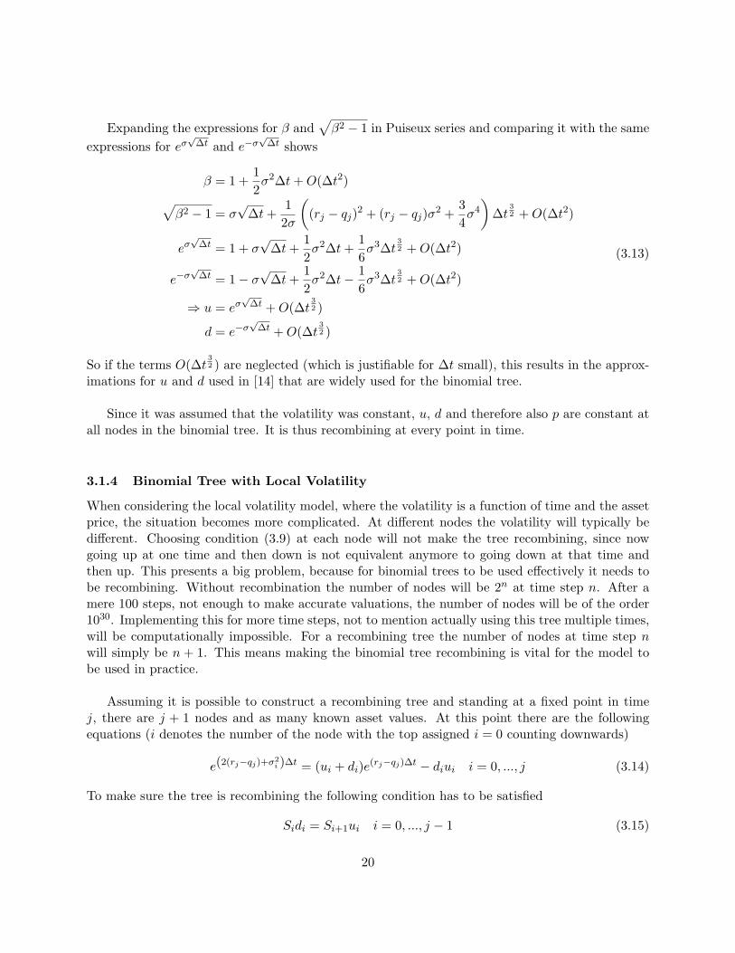
(3.13)

So if the terms O(∆t32 ) are neglected (which is justifiable for ∆t small), this results in the approx-

imations for u and d used in [14] that are widely used for the binomial tree.

Since it was assumed that the volatility was constant, u, d and therefore also p are constant atall nodes in the binomial tree. It is thus recombining at every point in time.

3.1.4 Binomial Tree with Local Volatility

When considering the local volatility model, where the volatility is a function of time and the assetprice, the situation becomes more complicated. At different nodes the volatility will typically bedifferent. Choosing condition (3.9) at each node will not make the tree recombining, since nowgoing up at one time and then down is not equivalent anymore to going down at that time andthen up. This presents a big problem, because for binomial trees to be used effectively it needs tobe recombining. Without recombination the number of nodes will be 2n at time step n. After amere 100 steps, not enough to make accurate valuations, the number of nodes will be of the order1030. Implementing this for more time steps, not to mention actually using this tree multiple times,will be computationally impossible. For a recombining tree the number of nodes at time step nwill simply be n + 1. This means making the binomial tree recombining is vital for the model tobe used in practice.

Assuming it is possible to construct a recombining tree and standing at a fixed point in timej, there are j + 1 nodes and as many known asset values. At this point there are the followingequations (i denotes the number of the node with the top assigned i = 0 counting downwards)

e(2(rj−qj)+σ2i )∆t = (ui + di)e(rj−qj)∆t − diui i = 0, ..., j (3.14)

To make sure the tree is recombining the following condition has to be satisfied

Sidi = Si+1ui i = 0, ..., j − 1 (3.15)

20

This means that at each point in time there are 2j+ 1 equations for 2j+ 2 unknowns, which meansthat typically this system can be solved, leaving one degree of freedom. By the very constructionof the tree it is ensured that the tree is recombining.

Using the degree of freedom to takedk = u−1

k (3.16)

at some node k there is a simple algorithm to construct the tree to value European options.

3.1.5 Algorithm

At time step j, there are j+1 nodes, i denotes the number of the node, and σi is the local volatilityat time j andnode i.

1. Calculate uk and dk with the original formula for the standard recombining binomial tree(3.12) because of assumption (3.16)

2. Calculate dk−1 from the recombining condition (3.15)

3. Calculate uk−1 from (3.14)

uk−1 =e(2(rj−qj)+σ2

i )∆t − dk−1e(r−q)∆t

e(rj−qj)∆t − dk−1

(3.17)

4. Repeat steps 2 and 3 for k − 2, .., 0

5. Calculate uk+1 from the recombining condition (3.15)

6. Calculate dk+1 from (3.14)

dk+1 =uk+1e

(rj−qj)∆t − e(2(rj−qj)+σ2i )∆t

uk+1 − e(rj−qj)∆t(3.18)

7. Repeat steps 5 and 6 for k + 2, ..., j

8. Put payoff values in tree at maturity, work backwards discounting the value of the option,where the transition probabilities are given by (3.5)

3.1.6 Instability of the Binomial Tree

When the binomial tree with local volatility, as described in the previous section, is implementeda major problem is encountered. For low values of the maximum amount of steps n, eg n < 80, inthe tree the model is relatively stable and seems to work reasonably well. To improve the accuracyof the model however more time steps are needed. When this is done the model becomes veryunstable. At some points in the tree the values for u and d start to oscillate (as is shown in 8.2.3).

21

This oscillation results in the fact that at some nodes u is smaller than d, resulting in irregulartrees for the asset price. This behaviour depends on the choice of k in (3.16). When k is chosen tobe 1 (the upper node), the tree becomes very unstable for n > 80. The optimal choice for k seemsto be to take k in the middle of the tree branch k = [ j2 ] (the square brackets denote rounding),where the tree becomes very unstable for around n > 100.

For some plain vanilla European options the model seems to give a reasonably well approxi-mation for the option price. However, since the model is unstable, it is impossible to check theaccuracy of the model sufficiently. Furthermore, given the irregular behaviour of the tree, it is im-possible to predict if this model is in any way useful when dealing with American or exotic options.

3.2 The Logarithmic Binomial Tree

One possible solution to remedy the instability of the standard binomial tree with local volatilitymay be to use a logarithmic binomial tree where the logarithmic values of the asset price and uand d are used. Maybe the different numerical behaviour of these variables will lead to increasedstability of the model.

3.2.1 Continuous Time

From (3.2) follow the equations for the mean and variance in continuous time

d lnSt = (rt − qt −12σ2)dt+ σdWt

lnSt = lnS0 +∫ t

t0

(rs − qs)ds−12σ2(t− t0) + σWt

(3.19)

or in the language of the binomial tree with time nodes j and j + 1

lnSj+1 = lnSj + (rj − qj −12σ2)∆t+ σ∆Wt (3.20)

Giving the mean and variance of the logarithm of the asset price at time node j + 1 as seen from j

E[lnSj+1] = lnSj + (rj − qj −12σ2)∆t

Var[lnSj+1] = σ2∆t(3.21)

3.2.2 Discrete Time

In discrete timeE[lnSj+1] = p ln(uSj) + (1− p) ln(dSj)

= lnSj + p lnu+ (1− p) ln d

E[(lnSj+1)2] = p ln2(uSj) + (1− p) ln2(dSj)

= p (lnu+ lnSj)2 + (1− p) (ln d+ lnSj)

2

= ln2 Sj + p ln2 u+ 2p lnu lnSj + (1− p) ln2 d+ 2(1− p) ln d lnSj

(3.22)

22

Leading to

Var[lnSj+1] = E[(lnSj+1)2]− (E[lnSj+1])2

= ln2 Sj + p ln2 u+ 2p lnu lnSj + (1− p) ln2 d+ 2(1− p) ln d lnSj− (ln2 Sj + 2p lnSj lnu+ 2(1− p) lnSj ln d+ p2 ln2 u

+ 2p(1− p) lnu ln d+ (1− p)2 ln2 d)

= (p− p2) ln2 u+ [(1− p)− (1− p)2] ln2 d− 2p(1− p) lnu ln d

= p(1− p)(ln2 u− 2 lnu ln d+ ln2 d)

= p(1− p) ln2 u

d

(3.23)

So the result of mean matching is

(rj − qj −12σ2)∆t = p lnu+ (1− p) ln d

⇒ p =(rj − qj − 1

2σ2)∆t− ln d

lnu− ln d

(3.24)

And for variance matching

σ2∆t = p(1− p) ln2 u

d

=

[(rj − qj − 1

2σ2)∆t− ln d

lnu− ln d

][lnu− (rj − qj − 1

2σ2)∆t

lnu− ln d

]ln2 u

d

= (rj − qj −12σ2)∆t[lnu+ ln d]− lnu ln d− (rj − qj −

12σ2)2(∆t)2

(3.25)

When choosing d = u−1 ⇒ ln d = − lnu at some node k, it yields

σ2∆t = ln2 uk − (rj − qj −12σ2)2(∆t)2

⇒ lnuk =

√σ2∆t+ (rj − qj −

12σ2)2(∆t)2

(3.26)

Which gives the same result as before if expanded in a Puiseux series

e

qσ2∆t+(rj−qj− 1

2σ2)2(∆t)2 = 1 + σ

√∆t+

12σ2∆t+O

(∆t

32

)⇒ uk = eσ

√∆t +O

(∆t

32

) (3.27)

For the logarithmic binomial tree with local volatility to be recombing, the following conditionneeds to be satisfied

lnSi + ln di = lnSi+1 + lnui+1 (3.28)

23

3.2.3 Algorithm

The algorithm for the logarithmic binomial tree is not that different from the one for the standardbinomial tree.

1. Calculate lnuk and ln dk for some fixed k from (3.26) and the condition that ln dk = − lnuk

2. Calculate ln dk−1 from the recombining condition (3.28)

3. Calculate lnuk−1 from (3.25)

lnuk−1 = (rj − qj −12σ2k−1)∆t−

σ2k−1∆t

ln dk−1 − (rj − qj − 12σ

2k−1)∆t

(3.29)

4. Repeat steps 2 and 3 for k − 2, .., 0

5. Calculate lnuk+1 from the recombining condition (3.28)

6. Calculate ln dk+1 from (3.25)

ln dk+1 =σ2k+1∆t

(rj − qj − 12σ

2k+1)− lnuk+1

+ (rj − qj −12σ2k+1)∆t (3.30)

7. Repeat steps 5 and 6 for k + 2, ..., j

8. Put payoff values in tree at maturity, work backwards discounting the value of the option,where the transition probabilities are known by (3.24)

3.2.4 Instability of the Logarithmic Binomial Tree

Unfortunately the logarithmic binomial tree exhibits the same unstable behaviour as the normalbinomial tree (although it behaves slightly better, see 8.2.4). In both cases no adjustments can bemade to counter the instability while keeping the tree recombining since there is only one degree offreedom at each time step, which needs to establish a relation between two variables at one node. Itseems that more degrees of freedom are needed to get a stable model. A model with more degreesof freedom is the trinomial tree model, which is the subject of the next section.

24

4 Trinomial Trees

The principles of the trinomial tree are the same as those of the binomial tree, the only differencebeing that at each node there are three possibilities for the next time step, Su, Sm and Sd, insteadof two. The basic equations needed for the construction of the trinomial tree are derived in 4.1.Two different methods of constructing the trinomial tree are described in 4.2 and 4.3. Dividends?

ZZZZZZZZ

uS

pu

1− pu − pd

pd

ZZZZZZZZ

uSu

Sm

Sd

ZZZZZZZZ

u

ZZZZZZZZ

u

u

u

u

u

u4.1 Basic Equations

Again the main equations are derived by equating the mean and variance to the values obtainedfrom the continuous time analysis. For the trinomial tree at each time the top node is denoted by0 and, since there are 2j + 1 nodes at time j, the bottom node is denoted by 2j.

E[Sj+1] = puSu + (1− pu − pd)Sm + pdSd

E[S2j+1] = puS

2u + (1− pu − pd)S2

m + pdS2d

Var[Sj+1] = E[S2j+1]− (E[Sj+1])2

= pu(Su − Sm)2 + pd(Sm − Sd)2 − (pu(Su − Sm)− pd(Sm − Sd))2

(4.1)

Matching mean and variance gives (using the notation of the binomial tree)

For i = 0, ..., 2j

e(rj−qj)∆t = pu,iui + (1− pu,i − pd,i)mi + pd,idi

e2(rj−qj)∆t(eσ

2i∆t − 1

)= pu,i(ui −mi)2 + pd,i(mi − di)2

− (pu,i(ui −mi)− pd,i(mi − di))2

(4.2)

25

To make the tree recombining it must be ensured that the following conditions hold

For i = 0, ..., 2j − 1miSi = ui+1Si+1

diSi = mi+1Si+1

(4.3)

Resulting in 4j + 2 equations from mean and variance matching and 4j equations from therecombining conditions. Since there are 5(2j + 1) unknowns, there are 2j + 3 degrees of freedom.These extra degrees of freedom with respect to the binomial tree will help solve the problems ex-perienced with that model.

The main problem with the binomial tree used with the local volatility model is the instabilityof the stock tree. At some points the values for ui,j and di,j began to oscillate, leading to situationswhere ui,j < 1 such that Su < Sd mangling the shape of the tree (if many time steps are used it caneven lead to ui,j < 0 leading to negative asset prices). In the trinomial tree this can be remedied bychoosing certain values for mi,j (using 2j+1 degrees of freedom). It is chosen to keep mi,j constantover all nodes i, simply denoting it by mj . The time dependency of mj will be discussed shortly.

Together with the recombining conditions (4.3) this leads to a robust tree, where Sd < Sm < Suis guaranteed (and negative assets prices are also avoided). Since this fixates almost all the pointsof the tree, the two remaining degrees of freedom are needed at the first and last node at each pointin time.

4.2 Fixing u and d

Since m is already fixed it seems obvious to use the remaining degrees of freedom to fix u and d.Most of these values are already fixed by the recombining conditions and the choice for fixing mj .Denoting the time step at one node by j, and remembering that by definition Si+1,j+1 is at thesame height as Si,j and i is counting down from the top to the bottom node, it follows from (4.3)that

ui+1,j+1 =Si+1,j+2

Si+1,j+1

=Si,j+1mi,j+1

Si,jmi,j

= ui,jmj+1

mj

(4.4)

Also at the last node u2j+2,j+1 is known by

u2j+2,j+1 =S2j+2,j+2

S2j+2,j+1

=S2j,jm2j,jm2j+1,j+1

S2j,jd2j,j

=mjmj+1

d2j,j

(4.5)

26

The equations for di+1,j+1 and d0,j+1 are comparable.

di+1,j+1 = di,jmj+1

mj

d0,j+1 =mjmj+1

u0,j

(4.6)

So the whole tree can be fixed by using the two remaining degrees of freedom to fix u0 and d2j

at each point in time j.The transition probabilities are derived from the first of (4.2)

pu,i =e(rj−qj)∆t + pd,i(mj − di)−mj

ui −mj

pd,i =e(2(rj−qj)+σ2

i )∆t − e(rj−qj)∆t(ui +mj) + uimj

(ui − di)(mj − di)

⇒ pu,i =e(2(rj−qj)+σ2

i )∆t − e(rj−qj)∆t(di +mj) + dimj

(ui −mj)(ui − di)⇒ pm,i = 1− pu,i − pd,i

=e(rj−qj)∆t(ui + di)− uidi − e(2(rj−qj)+σ2

i )∆t

(ui −mj)(mi − di)

(4.7)

4.2.1 Negative Probabilities

From the construction of the trinomial tree it is not guaranteed that the probabilities in (4.7) arebetween 0 and 1, and therefore may not be actual probabilities. Since all u’s and d’s are essentiallyfixed from the start, it is obvious they are chosen in a way such that ui > mi > di. This meansthat all the denominators in (4.7) are larger than zero. Temporarily denoting the numerator of pd,iby N , ensuring that pd,i ≥ 0 means N ≥ 0. Using that eσ

2i∆t ≥ 1, because σi ≥ 0, gives

N = e(2(rj−qj)+σ2i )∆t − e(rj−qj)∆t(ui +mj) + uimj

≥ e2(rj−qj)∆t − e(rj−qj)∆t(ui +mj) + uimj

=(e(rj−qj)∆t − ui

)(e(rj−qj)∆t −mj

) (4.8)

So if it is chosen to let mj = e(rj−qj)∆t, this means N ≥ 0 and thus pd,i ≥ 0. Expressions (4.7) canthus be written as

pu,i =e2(rj−qj)∆t

(eσ

2i∆t − 1

)(ui − e(rj−qj)∆t

)(ui − di)

pd,i =e2(rj−qj)∆t

(eσ

2i∆t − 1

)(ui − di)

(e(rj−qj)∆t − di

)pm,i =

e(rj−qj)∆t(ui + di)− uidi − e(2(rj−qj)+σ2i )∆t(

ui − e(rj−qj)∆t) (e(rj−qj)∆t − di

)(4.9)

27

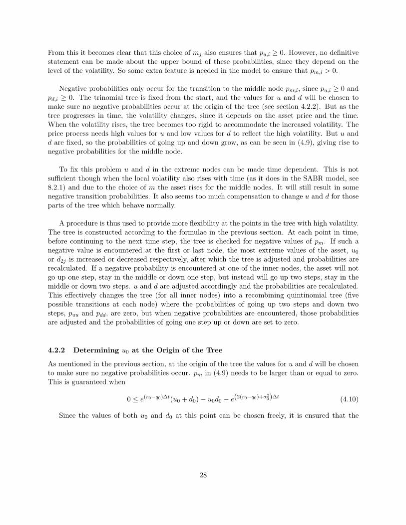
From this it becomes clear that this choice of mj also ensures that pu,i ≥ 0. However, no definitivestatement can be made about the upper bound of these probabilities, since they depend on thelevel of the volatility. So some extra feature is needed in the model to ensure that pm,i > 0.

Negative probabilities only occur for the transition to the middle node pm,i, since pu,i ≥ 0 andpd,i ≥ 0. The trinomial tree is fixed from the start, and the values for u and d will be chosen tomake sure no negative probabilities occur at the origin of the tree (see section 4.2.2). But as thetree progresses in time, the volatility changes, since it depends on the asset price and the time.When the volatility rises, the tree becomes too rigid to accommodate the increased volatility. Theprice process needs high values for u and low values for d to reflect the high volatility. But u andd are fixed, so the probabilities of going up and down grow, as can be seen in (4.9), giving rise tonegative probabilities for the middle node.

To fix this problem u and d in the extreme nodes can be made time dependent. This is notsufficient though when the local volatility also rises with time (as it does in the SABR model, see8.2.1) and due to the choice of m the asset rises for the middle nodes. It will still result in somenegative transition probabilities. It also seems too much compensation to change u and d for thoseparts of the tree which behave normally.

A procedure is thus used to provide more flexibility at the points in the tree with high volatility.The tree is constructed according to the formulae in the previous section. At each point in time,before continuing to the next time step, the tree is checked for negative values of pm. If such anegative value is encountered at the first or last node, the most extreme values of the asset, u0

or d2j is increased or decreased respectively, after which the tree is adjusted and probabilities arerecalculated. If a negative probability is encountered at one of the inner nodes, the asset will notgo up one step, stay in the middle or down one step, but instead will go up two steps, stay in themiddle or down two steps. u and d are adjusted accordingly and the probabilities are recalculated.This effectively changes the tree (for all inner nodes) into a recombining quintinomial tree (fivepossible transitions at each node) where the probabilities of going up two steps and down twosteps, puu and pdd, are zero, but when negative probabilities are encountered, those probabilitiesare adjusted and the probabilities of going one step up or down are set to zero.

4.2.2 Determining u0 at the Origin of the Tree

As mentioned in the previous section, at the origin of the tree the values for u and d will be chosento make sure no negative probabilities occur. pm in (4.9) needs to be larger than or equal to zero.This is guaranteed when

0 ≤ e(r0−q0)∆t(u0 + d0)− u0d0 − e(2(r0−q0)+σ20)∆t (4.10)

Since the values of both u0 and d0 at this point can be chosen freely, it is ensured that the

28

above inequality is satisfied. For instance if d0 = m20

u0= 1

u0e2(r0−q0)∆t then

0 ≤ u0, e(r0−q0)∆t +

1u0e3(r0−q0)∆t − e2(r0−q0)∆t − e(2(r0−q0)+σ2

0)∆t

0 ≤ u20 − u0e

(r0−q0)∆t(eσ

20∆t + 1

)+ e2(r0−q0)∆t

⇒ u0 ≥ umin :=12e(r0−q0)∆t

(eσ

20∆t + 1 +

√(eσ

20∆t + 1

)2− 4

) (4.11)

The other solution for u0 would require it to be less than a value which is typically less than 1, andis therefore discarded.

Different choices for u0 can be made as long as (4.11) is satisfied. A large value will make thetree wider, ensuring that negative probabilities will occur as little as possible. However, it givesrise to more inaccuracy. A possible reason for this can be that when the tree is wider there willbe fewer distinct values at maturity in that part that matters most: the middle part where theprobability of ending up in that part of the tree is largest. Since these values are the most likelyto occur and therefore contribute the most to the option value, having fewer of these value shouldlead to more imprecision. Therefore, to get the best result, the choice is made to put u0 = umin.

4.2.3 Implementing a Cutoff for High Volatilities

Another aspect that has to be considered is what happens in the tree when the asset price becomesvery large. In some models, including the SABR model depending on the specific parameters, thelocal volatility is increasing in the asset price. In the trinomial tree, as indeed is also the case inthe binomial tree, the values at the top of the tree become very large. If the local volatility surfaceis extrapolated to these prices, large volatilities can occur. This leads to negative probabilitiesfor the middle nodes even after adjusting u by large amounts. This causes serious delay in thecomputational time and leads to a general breakdown of the model and should thus be avoided.

The choice is made to implement a cutoff value for the asset dependency of the local volatility.Above some value for the asset price, for the calculation of the local volatility it is assumed the assetprice is equal to this cutoff value. This removes the asset dependency above the cutoff value, whilekeeping the time dependency. A natural question is if this can be done and if it will compromisethe accuracy of the model. To answer this question the effect of this cutoff value is determined byimplementing the trinomial tree for a large variety of cutoff values and strike prices (with maturityof 1 year and 1000 time steps). This results in two observations:

• Placing the cutoff value below 3S0 results in significant variations of the order of a few cents.

• For a cutoff value above 3S0, the cutoff value does not change the modeled price by morethan a tenth of a cent in the most extreme case.

These observations suggest that as long as the cutoff value is implemented at a relatively high value(≥ 3S0) the cutoff does not affect the option price significantly and therefore will not cause anysignificant problems.

29

4.2.4 Algorithm

At the origin of the tree:

1. Fix u0 = umin such that (4.11) is satisfied. Then fix m0 = e(r0−q0)∆t and d0 = m20

u0

2. Calculate the transition probabilities from (4.9)

3. Calculate the tree at time step 1

For all time steps j ≥ 1:

4. Fix u0,j and d2j,j . The other u’s and d’s are known from (4.4), (4.5) and (4.6)

5. Calculate tree values for time j + 1

6. Calculate the transition probabilities from (4.9)

7. Check for negative probabilities at each node i = 0, ..., 2j

8. If pm,0,j < 0

• Increase u0,j

• Start over from step 5

9. If pm,2j,j < 0

• Decrease d2j,j

• Start over from step 5

10. If pm,i,j < 0 for i /∈ 0, 2j

• uui,j = Si−1,j+1

Si,j

ddi,j = Si+3,j+1

Si,j

• Set pu,i,j = pd,i,j = 0

• Calculate puu,i,j , pm,i,j and pdd,i,j from (4.9) with uui,j and ddi,j instead of ui,j and di,j

• Start over from step 5

11. Increase time step and repeat steps 4-10 as long as the time of maturity is not reached

12. Put payoff values in the tree at maturity, work backwards discounting the value of the option(let V denote the value of the option)

Vi,j = e−rj∆t(puu,i,jVi−1,j+1 + pu,i,jVi,j+1 + pm,i,jVi+1,j+1 + pd,i,jVi+2,j+1 + pdd,i,jVi+3,j+1)(4.12)

30

4.3 Fixing Probabilities

The choice to be made at the end of 4.1 was what to do with the two remaining degrees of freedom,to evaluate the most extreme nodes. In the previous section these degrees were used to fix u andd. Although this is the most logical choice since the other degrees of freedom were used to fixthe values for m, it is not perfect, since it sometimes results in negative transition probabilitiesfor the middle nodes. Another possibility for using the two remaining degrees of freedom is to fixthe transition probabilities at these extreme nodes. This will lead to slightly more complicatedformulas but since it puts restrictions on the probabilities and lets u or d adjust in these points,this will sometimes lead to fewer problems with negative probabilities.

These probabilities are fixed by (omitting the time subscript)

pu,0 = pd,2j = pf (4.13)

4.3.1 Origin of the Tree

At the first node of the tree there are no recombining conditions. Equations (4.2) need to be solvedfor u0 and d0. Both probabilities are fixed since 2j + 1 = 1. The first of these equations gives

d0 =e(rj−qj)∆t − pu,0u0 − (1− pu,0 − pd,0)mj

pd,0(4.14)

Plugging this into the second equation

e2(rj−qj)∆t(eσ

20∆t − 1

)= pu,0(u0 −mj)2 + pd,0

(mj −

e(rj−qj)∆t − pu,0u0 − (1− pu,0 − pd,0)mj

pd,0

)2

−[pu,0(u0 −mj)−

(mjpd,0 − (e(rj−qj)∆t − pu,0u0 − (1− pu,0 − pd,0)mj

)]2

= pu,0(u0 −mj)2 +1pd,0

(pu,0(u0 −mj) +

(mj − e(rj−qj)∆t

))2−(e(rj−qj)∆t −mj

)2

= pu,0(u0 −mj)2 −(e(rj−qj)∆t −mj

)2

+1pd,0

[p2u,0(u0 −mj)2 + 2pu,0(u0 −mj)(mj − e(rj−qj)∆t) + (mj − e(rj−qj)∆t)2

]=

(pu,0 +

p2u,0

pd,0

)(u0 −mj)2 + 2

pu,0pd,0

(u0mj − u0e

(rj−qj)∆t −m2j +mje

(rj−qj)∆t)

+1− pd,0pd,0

(e(rj−qj)∆t −mj)2

(4.15)

31

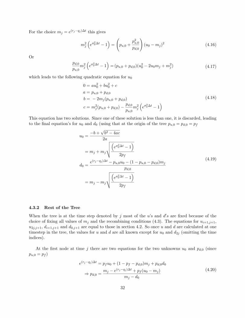
For the choice mj = e(rj−qj)∆t this gives

m2j

(eσ

20∆t − 1

)=

(pu,0 +

p2u,0

pd,0

)(u0 −mj)2 (4.16)

Orpd,0pu,0

m2j

(eσ

20∆t − 1

)= (pu,0 + pd,0)(u2

0 − 2u0mj +m2j ) (4.17)

which leads to the following quadratic equation for u0

0 = au20 + bu2

0 + c

a = pu,0 + pd,0

b = − 2mj(pu,0 + pd,0)

c = m2j (pu,0 + pd,0)−

pd,0pu,0

m2j

(eσ

20∆t − 1

) (4.18)

This equation has two solutions. Since one of these solution is less than one, it is discarded, leadingto the final equation’s for u0 and d0 (using that at the origin of the tree pu,0 = pd,0 = pf

u0 =−b+

√b2 − 4ac

2a

= mj +mj

√√√√(eσ20∆t − 1

)2pf

d0 =e(rj−qj)∆t − pu,0u0 − (1− pu,0 − pd,0)mj

pd,0

= mj −mj

√√√√(eσ20∆t − 1

)2pf

(4.19)

4.3.2 Rest of the Tree

When the tree is at the time step denoted by j most of the u’s and d′s are fixed because of thechoice of fixing all values of mj and the recombining conditions (4.3). The equations for ui+1,j+1,u2j,j+1, di+1,j+1 and d0,j+1 are equal to those in section 4.2. So once u and d are calculated at onetimestep in the tree, the values for u and d are all known except for u0 and d2j (omitting the timeindices).

At the first node at time j there are two equations for the two unknowns u0 and pd,0 (sincepu,0 = pf )

e(rj−qj)∆t = pfu0 + (1− pf − pd,0)mj + pd,0d0

⇒ pd,0 =mj − e(rj−qj)∆t + pf (u0 −mj)

mj − d0

(4.20)

32

and

e2(rj−qj)∆t(eσ

20∆t − 1

)= pf (u0 −mj)2 + pd,0(mj − d0)2 − (pf (u0 −mj)− pd,0(mj − d0))2

= pf (u20 − 2u0mj +m2

j ) + (mj − e(rj−qj)∆t + pf (u0 −mj))(mj − d0)

−(pf (u0 −mj)− [mj − e(rj−qj)∆t + pf (u0 −mj)]

)2

= pf (u20 − u0mj − u0d0 +mjd0)

+(mj − e(rj−qj)∆t

)(mj − d0)−

(e(rj−qj)∆t −mj

)2

(4.21)

Or for mj = e(rj−qj)∆t

m2j

pf

(eσ

20∆t − 1

)= u2

0 − u0(mj + d0) +mjd0 (4.22)

Resulting again in a quadratic equation for u0, where only the value bigger than 1 is considereda valid solution

0 = au20 + bu0 + c

a = 1b = −(mj + d0)

c = mjd0 −m2j

pf

(eσ

20∆t − 1

)⇒ u0 =

−b+√b2 − 4ac

2a

(4.23)

The same analysis holds for d2j where pd,2j = pf and u2j are known

e(rj−qj)∆t = pu,2ju2j + (1− pu,2j − pf )mj + pd,2jd2j

⇒ pu,2j =e(rj−qj)∆t −mj + pf (mj − d2j)

u2j −mj

(4.24)

e2(rj−qj)∆t(eσ

22j∆t − 1

)= pu,2j(u2j −mj)2 + pf (mj − d2j)2

− (pu,2j(u2j −mj)− pf (mj − d2j))2

=(e(rj−qj)∆t + pf (mj − d2j)−mj

)(u2j −mj)

+ pf (m2j − 2mjd2j + d2

2j)− (e(rj−qj)∆t −mj)2

= pf (d22j − d2jmj +mju2j − d2ju2j)

+(e(rj−qj)∆t −mj

)(u2j −mj)− (e(rj−qj)∆t −mj)2

(4.25)

Or for mj = e(rj−qj)∆t

m2j

pf

(eσ

22j∆t − 1

)= d2

2j − d2j(mj + u2j) +mju2j (4.26)

33

The only viable solution for this equation is the one that is less than one

0 = ad22j + bd2j + c

a = 1b = −(mj + u2j)

c = mju2j −m2j

pf

(eσ

22j∆t − 1

)⇒ d2j =

−b−√b2 − 4ac

2a

(4.27)

The transition probabilities can then be found by the equations (4.9), giving all the necessaryequations for building the trinomial tree and valuing options on it.

4.3.3 Negative Probabilities and Cutoff

When the last two degrees of freedom for the trinomial tree were used to fix the values for u andd and the extreme nodes, at some nodes negative transition probabilities appeared for the middletransition. The suspicion was that this was caused by a lack of flexibility in the tree. The treewith fixed probabilities at the extreme nodes is more flexible and can therefore better handle thechanges in the local volatility.

One consequence is that the values for the asset at the top of the tree increase significantly. Thisdoes not seem to result in bigger inaccuracies of the option price and is therefore not deemed tobe important. Another consequence is that when the tree is used with the SABR implied volatilitysurface as an input 8.2.1, it results in negative probabilities far fewer times than when u and d werefixed. To be more precise: only for relatively high values for pfixed do negative probabilities arise.For plain vanilla options with strike price K = S0 and T = 1 this maximum acceptable value forpfixed is 45.7% for 100 time steps and declines almost linearly to 44.9% for 1000 time steps. Belowthese values no negative probabilities arise, resulting in a ‘cleaner’ model. However, this behaviourdepends on the shape of the implied volatility surface, so no definite preference for one of bothversions of the tree can be given.

The exact choice of pfixed does not affect the price significantly. Only at very low values (lessthan 10%) and few time steps in the tree (less than 200) do significant deviations occur. The choiceis made to let pfixed = 30%. There is no significant difference in computational time between themodel where u and d are fixed and when the probabilities are fixed.

When implementing this model for the trinomial tree again a cutoff value for the local volatilityis used as described in 4.2.3.

For a numerical comparison between the two versions of the tree see 8.2.5. Numerical resultsdescribing the accuracy of the tree developed in this section for valuing European options can befound in 8.2.6. American options are considered in 8.2.8.

34

4.3.4 Algorithm

1. At the first node of the tree pu and pd are fixed in advance. u0 and d0 can be calculatedaccording to (4.19)

2. At the next time steps the u’s and d’s are given by (4.4), (4.5) and (4.6)

3. The two remaining values u0,j+1 and d2j+2,j+1 can be calculated by (4.23) and (4.27)

4. Since the tree at time step j + 1 is now completely fixed the transition probabilities can becalculated from (4.9)

5. Repeat steps 2.-4. until the tree is complete

6. Put the payoff of the option to be priced in a seperate tree and use the transition probabilitiesto calculate the discounted expected payoff of the tree

35

5 Dividends

Up until now the effect of dividends on option pricing has been ignored. Since most assets on whichoptions are written do pay out dividends it is important to incorporate this into the pricing model.Dividends are payments by the issuer of a financial asset (the asset underlying the option) to theholder of the asset. In financial modelling it is usually assumed that the payment of a dividendamount leads to a decline in the asset’s price by the same amount. This relies on the assumption ofa frictionless market in which the transfer of dividends does not encounter obstacles such as taxesor transaction costs. It also assumes that, when considering equity shares, a certain amount of cashon the balance sheet of a company is valued at exactly the same value as when the amount is onthe shareholder’s bank account.

5.1 Kinds of Dividends

Although the word ‘dividend’ is only used for shares, equivalent principles hold for other assetclasses. The regular interest payments, known as coupons, to bondholders, act in exactly the sameway. For currency exchange options, the interest rate of the foreign currency behaves like a dividendpayment [39].

For practical reasons there is usually a difference between the date when for all trading purposesthe asset is assumed to pay out the dividend, the ex-dividend date, and the actual time of payment.After the ex-dividend date the holder of the underlying asset does not have a claim to the declareddividend. In this report the ex-dividend date is used as the payment date.

Three different forms of dividends can be distinguished: continuous, proportional and discrete.

Continuous dividends are the easiest to deal with. As can be seen from the formulae in thissection, the presence of a continuous dividend yield usually amounts in a simple reduction of theinterest rate. For options on equity shares this situation never occurs. There is no company in theworld that pays out continuous dividends. However it does occur for options on currency exchangerates. Since foreign interest rates can be continuous, continuous dividend yields will occur for cur-rency options .

Proportional dividends assume that paid out dividends are proportional to the underlying as-set’s price at the ex-dividend date. This is easy to implement, since it results in a reduction inthe value of the asset price at each node, by a fixed percentage. A radically different share pricescould change the decision by a listed company concerning its dividend policy, providing some logi-cal basis for the assumption of proportional dividends. However, in most cases dividend paymentsare announced in advance and subsequent changes in the share price do not affect the payments.Therefore in most models, discrete dividends are used.

Discrete dividends describe the real-world situation for options on equity shares. The timingand size of dividends are usually well known in advance. The size of the dividend is not a givendeterministic function of the share price, such as with proportional dividends. But due to theassumptions stated above, some dependency between the two does exist. Given the assumption

36

that at the ex-dividend date the share price declines by the dividend size some assumption has tobe made for the occassion when the dividend size is equal or larger than the share price. Negativeshare prices do not occur in reality, due to the limited liability provisions applicable to publiclyheld companies. Therefore the assumption is made, as it is in [56], that the dividend size is equalto the minimum of the stated dividend and the share price. When the share price falls below thedividend size at the ex-dividend date, it is assumed the company only pays out the amount equalto the share price, thereby reducing the share price to zero.

5.2 Direct Implementation

Discrete dividends add complexity to the pricing of options, that do not arise for continuous andproportional dividends. First consider the traditional Black-Scholes framework with a constantvolatility term. When working with binomial trees the u and d are fixed at the beginning andare, because the volatility is constant, constant over the whole tree. Incorporating a fall in theshare price at a specific point in time, reflecting the dividend payment, destroys the recombiningproperty of the tree. This is, for reasons given in 3.1.4, unacceptable. The problem arises becausefrom the dividend date forward, different values for u and d should be used from to make the treerecombining, which is not possible in this framework.

Arguably, more flexibility is present when using trinomial trees with local volatility. Somesmall adjustments in (4.4) and the equivalent equation for d can take care of the impact discretedividends have on the recombining property of the tree. Since recombination in the trinomial treeis imposed, this should not be a problem. Still, discrete dividends cannot be implemented in thisway. The reason is that for low values of the share price, which are always present in the lowerregion of the tree, the discrete dividend will cause the share price to go to zero. Since the shareprice increases to a higher node by multiplying by u, this means that when the share price hitszero, it will stay zero (a straightforward consequence of the adjusted geometric Brownian motionframework). This means that this part of the tree cannot possibly recombine with the non-zeropart of the tree. Therefore another method must be used to implement the impact of discretedividends on the option price.

5.3 Dividend Adjustments to Model

In the literature different methods are proposed on how to deal with discrete dividends.

One approach, known as the escrowed model, is to separate the dividends from the asset price[39]. Since the discrete dividends are deterministic, they can be valued simply by discounting theirvalue by the risk-free interest rate. Then the tree is built with the spot price of the asset minusthe present value of the future dividends at the start of the tree. As the escrowed model bringsthe dividends back to the current time, the forward model pushes the dividends forwards to thematurity date. In the forward model the value of the dividends are compounded by the risk-freeinterest rate and added to the strike value of the option [47]. A combination of the escrowed andthe forward model is proposed in [9], where the dividends closest to the current date are brought

37

backwards and the other ones are pushed forwards.

It seems these models work relatively well in the standard Black-Scholes environment for Euro-pean options, but they suffer from some logical flaws as is pointed out in [36, 56]. In the escrowedmodel the spot price of the underlying asset is adjusted by the dividends during the life of theoption. This results in a different price process than the one used in the forward model. It is there-fore not surprising that they lead to different values for path-dependent options [31]. Furthermoreit follows that different maturities imply different price processes, but it is clear that the pricedynamics of the asset do not depend on the particular options depending on it. A remedy for thiswould be to include all future dividends, but, as pointed out in [56], this is also unsatisfactory froma logical point of view since changes in dividends after the option’s maturity should not affect theoption price.

In a local volatility model modifying the spot price cannot be justified, since the local volatilitysurface is calculated with the current spot price. By adjusting the spot price it is not clear if thesame local volatility surface can be used. In making the decision if it can be used, an assumptionhas to be made on how the surface changes under spot price moves. There is no reason to assumethe surface depends on the asset’s spot price, but there is no guarantee that it doesn’t.

Since both the escrowed and the forward model compress all the dividends in one point they donot sufficiently incorporate the effects that the dividends will have on early exercise decisions. It iswell known that early exercise for American call options is only profitable just before the dividenddates [39]. By compressing all the dividends into one point, it removes the possible moments ofearly exercise from the tree. So American calls, and by similar reasoning puts, cannot be accuratelypriced using the escrowed or forward model.

5.4 The Vellekoop-Nieuwenhuis Method

The Vellekoop-Nieuwenhuis model [56], does not adjust the price process of the asset, but insteadadjusts the discounting process of the option on the tree. The tree is built without any dividends.The payoff can then be discounted in the normal way up until the last dividend date (which is thefirst that is encountered when working backwards). At these nodes, whose asset values are writtencollectively as S, the price of the option is a function of the asset price, f(S). But this is withoutdividends. At these nodes the asset price declines by the value of the dividend, d. So the correctprices at these nodes are actually f(S− d). Assuming that f is a continuous function, these valuescan be approximated by interpolating the values f(S) to f(S−d). Here it is assumed that the assetprice never becomes negative, so actually f(S) is interpolated onto f(max(S−d, 0)). Cubic splinesare used as the method of interpolation, in contrast to [56] where linear interpolation is used. Toavoid extrapolation the points f(S) are augmented by the point f(0). Since an asset price withvalue zero will always remain zero, this value can be easily determined for both the call and theput, both European and American. Then the option value can be discounted in the regular wayuntil a new dividend is encountered, at which point the same procedure is performed.

In the original article binomial trees are used, but, as is explicitly mentioned there, the methodcan also be applied to trinomial trees. A property that does not carry over unto the local volatility

38

model, is the convergence proof. One of the assumptions used in proving convergence, is that in theabsence of dividends uniform convergence exists. This is the case for trees with constant volatility,for which uniform convergence is proven [37]. A convergence result does not exist for trees withlocal volatility (yet), so convergence of the price obtained by the tree, to the true option price, isnot guaranteed.

5.5 Interest Rates

At all points in the preceding sections the interest rate was said to be a known deterministic functionof time. However this is not the way in which interest rates are observed in the market. Althoughit is easy to derive the interest rate function from market data, for completeness it is included inthis report.

Interest rates are observed indirectly in the market, they are derived from the price of risk-freebonds. A zero-coupon bond is a claim on a specific amount of cash in the future, without thepayment of intermediary amounts. Since it is risk free, the price is the amount discounted by therisk-free interest rate

p(t0, T ) = e−R(t0,T )(T−t0) (5.1)

where p(t0, T ) is the bond price at time t0 for a claim of 1 unit of cash at time T . R(t0, T ) is thebond’s yield, which can be easily calculated from bond prices. When this rate is used for otherpurposes than describing a bond, it is referred to as the spot interest rate for a certain maturity.Equal bonds with different maturities have different prices, and therefore different yields. Becausethe yield is a function of the time to maturity, it is usually called the yield curve. The time evolu-tion of the short interest rate can be derived from this yield curve.

The price of a risk-free bond can be written as the expected value of the discounted value ofthe 1 unit of cash at maturity. So when interest rates are deterministic

p(t0, T ) = E[e−R Tt0rsds|F0]

= e−

R Tt0rsds

(5.2)

By combining this equation with (5.1)∫ T

t0

rsds = R(t0, T )(T − t0)

rT =∂R(t0, T )

∂T(T − t0) +R(t0, T )

rt =∂R(t0, y)

∂y

∣∣∣∣∣y=t

(t− t0) +R(t0, t)

(5.3)

39

6 Delta Hedging

An essential practice for the option trading industry is hedging. The simplest version, delta hedging,is the subject of this section. In 6.1 delta hedging in the classical Black-Scholes framework ispresented. The minimum variance hedge is given in 6.2 and the hedge given by the local volatilitymodel, the local delta, is considered in 6.3.

6.1 Black-Scholes Framework

The most commonly known technique to ensure a trader with a long or short position of an optionagainst fluctuations in the price of the underlying asset is delta hedging. The total portfolio ismade delta-neutral by adding a certain amount of the asset. Thus if Π is the value of the portfolioand Black-Scholes is assumed

Π = VBS − S∆BS (6.1)

Then, the portfolio is hedged only at the point when the option position is taken, the delta of theoption can be calculated by equating the total delta of the portfolio to zero

∆BS =∂VBS

∂S(6.2)

This is the classic result, which holds in the Black-Scholes environment and would hold in the realmarkets if all prices were described by geometric Brownian motion. But when other models areused such as the local volatility model things change. When trying to fit specific model variablesα the following equation must be satisfied

V (S, t,K, T ) = VBS(S, t,K, T, α) (6.3)

Calculating the derivative of this equation results in

∂V

∂S=∂VBS

∂S+∂VBS

∂α

∂α

∂S

= ∆BS +∂VBS

∂α

∂α

∂S

(6.4)

Which is just a generalisation of the Black-Scholes model since in that model the second term inthe last equation would equal zero. The point this equation makes, is that different models lead todifferent delta hedges.

6.2 Minimum Variance Delta

Observing the statements above, [1] suggests defining a minimum variance (MV) delta that min-imises the quadratic covariation of the changes in the delta hedged portfolio Π with the changes inthe underlying asset. Setting this equal to zero

0 = dΠ · dS= (dV − dS∆MV) · dS

⇒ ∆MV =dV · dSdS · dS

(6.5)

40

Considering the local volatility model and using Ito gives

dV =∂V

∂SdS +

∂V

∂tdt+

∂V

∂σdσ +

12∂2V

∂S2dS · dS

+12∂2V

∂σ2dσ · dσ +

∂2V

∂S∂σdS · dσ

dσ =∂σ

∂SdS +

∂σ

∂tdt+

12∂2σ

∂S2dS · dS

dσ · dσ =∂σ

∂SdS · dS

dS · dσ =∂σ

∂SdS · dS

⇒ dV · dS =∂V

∂SdS · dS +

∂V

∂σdσ · dS

=(∂V

∂S+∂V

∂σ

∂σ

∂S

)dS · dS

(6.6)

this results in∆MV =

∂V

∂S+∂V

∂σ

∂σ

∂S(6.7)

This is an important adjustment to the normal delta, which is the first term on the right-handside of the equation above. It has been noticed that applying the normal delta for delta hedgingpurposes leads to inaccurate values of the delta [5, 12, 22]. It seems that to get good delta hedges inthe local volatility model, some sort of vega hedge (the sensitivity with respect to the volatility) hasto be incorporated to get good results [27]. These ad-hoc alterations are messy and seem to comefrom nowhere. But (6.7) suggests that this vega adjustment should have been incorporated all along.

6.3 Local Delta

As remarked in [16, 24, 55], volatility is usually negatively correlated to the asset price. Since plainvanilla options have positive vega’s, this would suggest that in general ∆L ≤ ∆BS. Although theMV delta is presented in a nice analytic form, for the local volatility model it cannot be used inthis way. The partial derivatives of the option value used in (6.7) are not known. Therefore thedelta for the local volatility delta will always be calculated numerically.

One of the criticisms of local volatility models is that it implies dynamics of the implied volatilitysurface that are not compatible with market practices [4, 34]. This behaviour is illustrated whenthe local volatility function is time independent and solely a function of the asset price. In [34]Hagan derived, by perturbation techniques, that the implied volatility at time t0 with asset priceS0 can then be approximated by

Σ(K,T ;S0) = σ

(12

[S0 +K])

(6.8)

which implies that as the spot of the asset moves up by ∆S

Σ(K,T ;S0 + ∆S) = σ

(12

[(S0 + ∆S) +K])

= σ

(12

[S0 + (K + ∆S)])

= Σ(K + ∆S, T ;S0) (6.9)

41

Suggesting that as the spot price moves up the implied volatility curve moves to the left, which,according to Hagan, is contrary to the experience of market participants. For this reason it isassumed that local volatility models give wrong greeks and therefore provide wrong hedges.

The reasoning of the critique above is, however, only justified if certain ‘stickiness’ assumptionshold, highlighting the importance of being aware of the different possible assumptions that can bemade.

6.3.1 Stickiness Assumptions

The term ‘sticky’ to describe the dynamics of the implied volatility curve (the cross section of theimplied volatility surface for a given maturity) was introduced in [17]. In general three differentstickiness assumptions can be made

• If the implied volatility curve does not change when the spot price of the underlying assetchanges the curve is said to be sticky-strike

Σ(K,T ;S0) = Σ(K,T ;S0 + ∆S) (6.10)

• If the implied volatility curve does not change when the spot price of the underlying assetchanges but the moneyness ( SK ) does not change the curve is said to be sticky-moneyness.

Σ(K,T ;S0) = Σ(K +K

S0∆S, T ;S0 + ∆S) (6.11)

• If the local volatility surface is assumed to be fixed, then the model is said to be modelconsistent

σ(S, t;S0) = σ(S, t;S0 + ∆S0)⇒ Σ(K,T ;S0) ≈ Σ(K + ∆S, T ;S0 −∆S)

(6.12)

From this it can be seen that Hagan’s critique only holds when one assumes that in reality theimplied volatility is sticky moneyness. However as pointed out in [27] and [49] this may not be thebest assumption in every market.

Sections 6.1 and 6.2 gave a theoretical description of calculating delta’s. In practice delta’s areusually calculated numerically. The simplest approach is by taking the central difference approxi-mation

∆(S0) =∂V (S0)∂S

≈ V (S0 + ∆S)− V (S0 −∆S)2∆S

(6.13)

where ∆S is some small change in S0. This approach, however, does not recognise the observationsmade about different stickiness assumptions. If a change in S0 changes the local volatility surface,the new perturbed option values (V (S0 +∆S) and V (S0−∆S)) should be calculated using the newlocal volatility surface. A more accurate numerical calculation of ∆(S0) would thus be (borrowingnotation from [27])

∆(S0) ≈ 12∆S

[V (S0 + ∆S, σ(Σ(K + α∆S, T ;S0 + β∆S);S0 + β∆S)

−V (S0 −∆S, σ(Σ(K − α∆S, T ;S0 − β∆S);S0 − β∆S)](6.14)

42

The sticky-strike assumption corresponds to α = 0, β = 1, sticky-moneyness to α = KS0

, β = 1and model consistent to α = 0, β = 0 (no change in the local volatility surface). Which one ofthese assumptions should be made is not clear a priori. If the local volatility function captures theactual diffusion process for the asset price, then it should remain constant, indicating the modelconsistent stickiness assumption is justified. There are, however, many indications that differentmarkets justify different stickiness assumptions [49]. [16] suggests that for equity markets andequity indices the model consistent assumption is the most natural.

6.3.2 Performance of Local Delta

The earliest comparison of the performance of local delta hedging versus Black-Scholes (or implied)delta hedging, suggests that the traditional BS delta performs best [24]. Most subsequent research[12, 13, 16, 55] concludes the opposite, although [16] provides a more nuanced picture. Since thelocal delta captures local information, the local delta should provide a better hedge. Given themultiple adjustments that are necessary to make the BS delta work accurately [5, 12, 22], the BSdelta does not inspire much confidence as a good hedge. The numerical results presented in section8.4.4 present a mixed picture.

43

7 Monte Carlo Simulations

The principle method of pricing options presented in this report is the trinomial tree. The reasonwhy Monte Carlo simulations are included is to compare the outcomes of the trinomial tree to areference value. For standard European options this reference value can be both the Black-Scholesformula, which provides a closed form formula for the option prices, and Monte Carlo simulations.For American options only the latter is available to generate reference values.

In Monte Carlo simulations the dynamics of the asset price under the risk neutral measure Q asgiven by (1.8) are simulated. By sampling a great number of paths an approximation is made forthe actual dynamics of the underlying asset. By calculating what the value of a particular optionwould be under many sample paths and then averaging the result, an approximation is made forthe expected discounted value of the payoff, thus giving an estimate for the option price underconsideration. The standard method is described in 7.1-7.3. Although the standard Monte Carlomethod can only be used for European options, it can be modified to accomodate other options(such as American and exotic options). To do this the method developed by Longstaff and Schwartz[43] is used, which is described in 7.4.

7.1 Creating Sample Paths

The dynamics as given in (1.8) are made by fixing S0 and discretising the equation into

St+∆t = St (1 + (rt − qt)∆t+ σ(t, St)∆Wt)

∆Wt = Wt+∆t −Wt ∼ N(0,∆t) =√

∆tN(0, 1)

St+∆t = St

(1 + (rt − qt)∆t+ σ(t, St) εt

√∆t) (7.1)

where εt ∼ N(0, 1) is distributed according to the standard normal distribution and independentsamples are used at different times.

7.2 Antithetic Sampling

The simulation of the function εt in (7.1) is the essential part in Monte Carlo simulation, sinceit is the only source of randomness, all the other values are deterministic. Thus making sure thesampling of this function as accurate as possible is of the utmost importance. A method that isused often to create better estimates, and which reduces the variance of the estimate, is antitheticsamples.

The standard normal distribution is symmetric. If φ is the probability density function of thestandard normal distribution this means that φ(x) = φ(−x). Thus when εt is simulated, it isequally likely to generate a sample value Xi as it is to get −Xi. To make ensure this property holdsexactly during the simulation, everytime a sample Xi is generated, the value −Xi (the antitheticsample) is used in another sample path, obtaining twice the number of sample paths.

Calculating the estimate for the option value and the confidence interval, relies on the StrongLaw of Large Numbers and the Central Limit Theorem. Let Yi be an option value calculated using

44

one sample path, and let Yi be the value calculated by the antithetic path. Then Yi and Yi arenot independent from each other, but each pair (Yi, Yi) is independent and identically distributed.This means that the average can be defined as

Y =1

2n

(n∑i=1

Yi +n∑i=1

Yi

)=

1n

n∑i=1

(Yi + Yi

2

)(7.2)

where n is the number of original samples that are generated and Yi+Yi2 are iid. So by the Law of

Large NumbersY → E[Y ] as n→∞ (7.3)

This ensures that eventually the average will converge to the actual option value.

By the Central Limit Theorem

Y − E[Y ]σ/√n→ N(0, 1) as n→∞

σ2 = Var(Y )(7.4)

Denoting the cumulative density function of the normal distribution by Φ, the 95% confidenceinterval will thus be given by

Y ± Φ−1(0.975)σ√n

(7.5)

Since Yi and Yi are negatively correlated, the variance of Y is smaller than if 2n samples ofYi would have been considered. As such antithetic sampling is known as a variance reductiontechnique. Other variance reduction techniques include control variates, stratified sampling andimportance sampling [33].

7.3 European Options

By calculating the payoff at maturity and discounting, the value of a standard European option canbe determined. This is a simple procedure, requiring few programming skills. The drawback is thata large amount of simulations (in the order of millions) have to be performed to get accurate results.The reason for this is that to get an accurate estimate for the price of an option, the probabilitydensity distribution of the asset price at maturity has to be determined. Both in the tree and inMonte Carlo simulations this is the essence of the method. In the tree however, many differentpossible outcomes are determined, each of which is assigned a probability value. In Monte Carlosimulations this probability is determined by looking at many different simulations. To accuratelyapproximate the probability density distribution at maturity, the number of simulations has to beof such a high order that highly unlikely outcomes are also represented in the sample. The resultof which is that although the concept of Monte Carlo simulations is simple, the execution can betime consuming.

Numerical results for valuing European options by Monte Carlo simulations can be found in8.2.7.

45

7.4 American Options

Since a European option can only be exercised at maturity, calculating the payoff is easy. For anAmerican option the situation is more complicated, since it can be exercised at each moment intime before maturity. Simulations for each infinitesimal time period is not practical, so the timepoints at which the American option can be exercised is limited to the discrete points in time usedin the simulation. In effect a Bermudan option is simulated, which is used as an approximation tothe American option.

A further complication is that it is usually not known when it is optimal to exercise the option.To determine whether it is optimal to exercise the option at a particular point in time the immediateexercise value should be compared to the expected value of continuing with the option, conditionalon the current state. So if j denotes the time step and Vj is the option value at that time

Vj = max(erj∆tE[Vj+1|Fj ], Ej) (7.6)

where Ej is the immediate exercise value. For the tree this was easy to calculate, since the valueE[Vj+1|Fj ] was known when discounting backwards from the transition probabilities. During aMonte Carlo simulation this is not the case. An approximation has to be made. The method usedhere is the commonly used Longstaff-Schwartz method [43]. At maturity the payoff of the optionis known. Working backwards the expected value of continuing with the option (the continuationvalue) is estimated from the discounted cash flows at later times. It is assumed that the continuationvalue can be estimated to be a linear combination of functions on the information at time j

E[Vj+1|Fj ] =N∑i=1

aiψi(Sj) (7.7)

where ψi are a set of deterministic functions, referred to as basis functions.

By taking a set of sample paths and regressing the discounted cash flows of future times ontothe basis functions the coefficients ai can be estimated. This is usually done in a least squares sense(the method is therefore usually denoted as the Least Squares Monte Carlo Method or LSM). Thisway an estimate of the continuation value can be made for each sample path, giving a criterion forearly exercise by comparing this value to the immediate exercise value.

7.4.1 Bias and Convergence of LSM

By approximating the American option with a Bermudan option a bias is introduced into the es-timation of the option value. Since a Bermudan option has less possibilities of early exercise, itsvalue is always less or equal to an American option with the same specifications. This low bias fromsub-optimal exercise is mentioned in the original Longstaff-Schwartz article and it is suggested thatthe estimated option value can never be be larger than the true option value because of this. This,however, is not all there is to it.

As noted in [30, 33] there is also a high bias. The LSM approximates the expected value of theoption at a later time conditional on the current information, by regressing the continuation value

46

on certain basis functions. These continuation values however, are obtained from information onthe future paths of the simulations. This seems like a clear violation of the measurability of theconditional expectation (Vj should be Fj-measurable, but now information from tj+1 is used). Byconsidering the future cash flows a superoptimal exercise strategy is employed. As a result the biasof the method is mixed. One could hope that the positive and negative bias somehow cancel eachother out, but there is no clear indication that this will indeed happen.

The LSM is similar to the method proposed by Tsitsiklis and Van Roy [53, 54], where the valuefunction is approximated instead of the continuation value, but Longstaff and Schwartz decided touse only those sample paths that were in the money for the regression, improving the efficiency ofthe algortihm. Convergence of LSM is studied in [11, 52, 60] were almost sure convergence of thealgorithm is shown as the number of basis functions and sample paths used go to infinity. Thisis proven for the algorithm given in the original article, which assumes constant volatility. It isthus not clear whether this method will converge to the real value of the option for a non-flat localvolatility surface. Increasing the amount of samples will usually reduce the variance and thus showssome convergence, but this does not necessarily improve the accuracy of the estimate.

Numerical results for valuing American options by Monte Carlo simulations can be found in8.2.8.

47

8 Numerical Results

8.1 Finite Differences Approximation for Derivatives

If an analytic expression exists for a differentiable function, the derivative can be calculated ana-lytically. But in most cases either there exists no such analytic expression or the expression is socomplicated that taking derivatives renders it impossible to get an analytic expression (as is thecase in the SABR model, see section 8.2.1).The finite differences approach is a numerical methodoften used to get approximating values for derivative values of a function for which values are knownon a fixed grid. The essence of this method is to approximate the given function with a ordinarypolynomial of order n. The factors of this polynomial can then be determined by consideringn + 1 values of the given function. The higher the order of the approximation, the higher the ac-curacy, but the more complicated the formulae. In this report the approximations are of the order 4.

Assume an equidistantly spaced grid with interpoint distances of ∆x, on which the functionu(x) is known at the grid points. For 4th order approximations, 5 points need to be considered,u0, u1, u2, u3 and u4, placed at x0 = 0, x1 = ∆x, x2 = 2∆x, x3 = 3∆x and x4 = 4∆x respectively.The polynomial approximation for the function and the first two derivatives is

u(x) ≈ c0 + c1x+ c2x2 + c3x

3 + c4x4

u′(x) ≈ c1 + 2c2x+ 3c3x2 + 4c4x

3

u′′(x) ≈ 2c2 + 6c3x+ 12c4x2

(8.1)

the first of which gives the following expressions for the known values of u

u0 ≈ c0

u1 ≈ c0 + c1∆x+ c2(∆x)2 + c3(∆x)3 + c4(∆x)4

u2 ≈ c0 + 2c1∆x+ 4c2(∆x)2 + 8c3(∆x)3 + 16c4(∆x)4

u3 ≈ c0 + 3c1∆x+ 9c2(∆x)2 + 27c3(∆x)3 + 81c4(∆x)4

u4 ≈ c0 + 4c1∆x+ 16c2(∆x)2 + 64c3(∆x)3 + 256c4(∆x)4

(8.2)

This system of five equations with five unknowns (the u’s and ∆x are known) can be solved toyield expressions for the polynomial constants

c0 ≈ u0

c1 ≈−25u0 + 48u1 − 36u2 + 16u3 − 3u4

12∆x

c2 ≈35u0 − 104u1 + 114u2 − 56u3 + 11u4

24(∆x)2

c3 ≈−5u0 + 18u1 − 24u2 + 14u3 − 3u4

12(∆x)3

c4 ≈u0 − 4u1 + 6u2 − 4u3 + u4

24(∆x)4

(8.3)

Once inserted into (8.1), these equations result in the approximations for the derivatives of u with

48

respect to the variable x in the points x0, x1, x2, x3 and x4.

u′(x0) ≈ −25u0 + 48u1 − 36u2 + 16u3 − 3u4

12∆x

u′′(x0) ≈ 35u0 − 104u1 + 114u2 − 56u3 + 11u4

12(∆x)2

u′(x1) ≈ −3u0 − 10u1 + 18u2 − 6u3 + u4

12∆x

u′′(x1) ≈ 11u0 − 20u1 + 6u2 + 4u3 − u4

12(∆x)2

u′(x2) ≈ u0 − 8u1 + 8u3 − u4

12∆x

u′′(x2) ≈ −u0 + 16u1 − 30u2 + 16u3 − u4

12(∆x)2

u′(x3) ≈ −u0 + 6u1 − 18u2 + 10u3 + 3u4

12∆x

u′′(x3) ≈ −u0 + 4u1 + 6u2 − 20u3 + 11u4

12(∆x)2

u′(x4) ≈ 3u0 − 16u1 + 36u2 − 48u3 + 25u4

12∆x

u′′(x4) ≈ 11u0 − 56u1 + 114u2 − 104u3 + 35u4

12(∆x)2

(8.4)

When approximating the values of derivatives in a gridpoint, it should be the most accuratewhen an equal amount of points on both sides are used for this procedure (i.e. the values forx2). These approximations are usually referred to as central differences. Since the derivation ofequations above only depends on the relative position of the x values with respect to each otherand not on their absolute position, the formulas hold on the entire grid. Therefore in all pointson the grid the central differences are used, except in the cases where there are not two gridpointson both sides of the point in which we are making approximations. In these boundary points theformulas with x1 and x3 are used when there is one gridpoint on one side of the point and the thosewith x0 and x4 when it is a true boundary point (i.e. on the edge of the grid).

Note that the variable x in these derivations is arbitrary, such that the formulae hold for deriva-tives with respect any variable, where the derivatives are made in a any direction on the grid. Forhigher order derivative approximations the expressions can be easily deduced from the expressionsabove. Mixed derivatives are slightly more complicated and deserve some more work. Since higherorder and mixed derivatives are not used in this report the formulae for these are not derived here.

8.2 SABR Model

As was seen in 2.3, to derive the local volatility surface implied volatilities are needed as an input.To check how well the methods presented in this report work, at first it is checked in an environmentwhere the implied volatility surface is known.

49

8.2.1 Theoretical Framework

In [34] the Stochastic-αβρ, or shortly SABR, model was derived in which the volatility functionwas assumed to be stochastic. The dynamics of the SABR model are given by

dFt = αtFβt dW

1t

dαt = ναtdW2t

dW 1t · dW 2

t = ρdt

(8.5)

Here Ft is the forward price, αt the volatility function with starting value α0 = α, ρ is the correlationbetween the two Brownian motions ad ν is the volatility of the volatility.

The SABR model has the advantage that there exists an analytic expression for the impliedvolatility as a function of the strike price K and the forward price f = F0 = Se(r0−q0)T . The bestresult would be a precise analytic expression for the local volatility function. In the SABR modelthe implied volatility is closely approximated by

Σ(f,K) ≈ α(fK)β−1

2

[1 +

(1− β)2

24ln2

(f

K

)+

(1− β)4

1920ln4

(f

K

)]−1(z

x(z)

)[

1 +

((1− β)2

24α2

(fK)1−β +14

ρβνα

(fK)(1−β)

2

+2− 3ρ2

24ν2

)τ

] (8.6)

where

z =ν

α(fK)

(1−β)2 ln

(f

K

)x(z) = ln

(√1− 2ρz + z2 + z − ρ

1− ρ

) (8.7)

which is derived in [34].

Since an analytic, closed form formula for the implied volatility exists, plugging it into (2.25)will result in an expression for the local volatility. However, it is easy to see that this formulawould be huge. Particularly the derivative with respect to T is large, rendering it impossible towork with. Programs such as Maple cannot handle it. Even the simpler approximating formula

Σ(f,K) ≈ α

f1−β

(1− 1

2[1− β − ρλ] ln

(K

f

)+

112[(1− β)2 + (2− 3ρ2)λ2

]ln2

(K

f

))(8.8)

proves to be unworkable for the same reasons. Therefore it is necessary to focus on numericalapproximations of (2.25).

A different approximation for the implied volatility surface is made in [6]. Just like (8.6) thisis an asymptotic expansion of the implied volatility surface with an error of O

(∆τ2

). From [48]

it becomes clear that the SABR model is better approximated by the function derived in [6] and

50

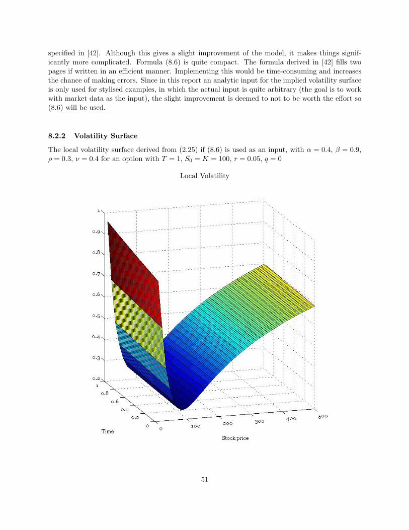
specified in [42]. Although this gives a slight improvement of the model, it makes things signif-icantly more complicated. Formula (8.6) is quite compact. The formula derived in [42] fills twopages if written in an efficient manner. Implementing this would be time-consuming and increasesthe chance of making errors. Since in this report an analytic input for the implied volatility surfaceis only used for stylised examples, in which the actual input is quite arbitrary (the goal is to workwith market data as the input), the slight improvement is deemed to not to be worth the effort so(8.6) will be used.

8.2.2 Volatility Surface

The local volatility surface derived from (2.25) if (8.6) is used as an input, with α = 0.4, β = 0.9,ρ = 0.3, ν = 0.4 for an option with T = 1, S0 = K = 100, r = 0.05, q = 0

Local Volatility

51

The local volatility exhibits a strong dependency on the underlying asset price. It goes to in-finity as the asset price approaches zero as can be seen from (8.6). The time dependency is lesspronounced, but the volatility is increasing in time, especially for small values of S.

8.2.3 Binomial Tree Instability

In section 3.1.6 the inherent instability of the binomial tree, as used with local volatility, wasdescribed. The main problem is that the value for u, d and p become highly irregular. As anexample the different values of u as they appear in a binomial tree with 100 time steps are plottedbelow as a function of the position in the tree. The underlying asset has initial value S0 = 100 andthe local volatility surface used is the one shown in 8.2.2. Since the values of u vary wildly thevalues are capped at 100 on the positive side (actual values attained were of the order 1020).

Values of u on tree

52

It should be noted that although this tree seems highly unstable (negative value for u are obvi-ously unrealistic), for European options it did result in prices closely resembling the Black-Scholesprices (differences of a few cents). For more time steps, needed to increase the accuracy, this wasnot the case.

8.2.4 Logarithmic Binomial Tree Instability

When the exact same local volatility as given in 8.2.2 is used for the logarithmic binomial tree,the same instability arises (as described in 3.2.4). It does behave slightly better than the regularbinomial tree, as can be seen in the graph below, which did not need to capped for large values aswas needed for the regular binomial tree. However, the large oscillations in the values for u and theoccurrence of negative values are clearly unacceptable in any model that tries to describe reality.

Values of u on tree

53

8.2.5 Comparison Between Fixing u and d and Fixing Probabilities

When constructing the trinomial tree in section 4 a choice had to be made what to do with thedegrees of freedom. Most were used to fix the increment of making the middle transition, for theremaining degrees two possible choices were presented, fixing u and d in 4.2, and fixing probabilitiesin 4.3. Both versions of the tree were said to have similar accuracies. The numerical comparison isgiven in the table below.

For different values of the number of steps in the tree a European call and put options withS0 = K = 100 are priced using both trees and compared to the Black-Scholes price. The differencesbetween the trees are equal for both call and put and are therefore only mentioned once per numberof time steps.

Black-Scholes: Call = 12.4707, Put = 7.5936

Time Steps Call/Put Tree pf Tree u and d Diff. Trees Diff./BS50 C 12.4597 12.4692 -9.46·10−3 -.0758 %

P 7.5826 7.5921 -.1245 %100 C 12.4809 12.4824 -1.55·10−3 -.0124 %

P 7.6038 7.6054 -.0204 %200 C 12.4711 12.4710 9.94·10−5 .0008 %

P 7.5941 7.5940 .0013 %300 C 12.4734 12.4650 8.32·10−3 .0667 %

P 7.5963 7.5880 .1096 %400 C 12.4694 12.4707 -1.21·10−3 -.0097 %

P 7.5924 7.5936 -.0160 %500 C 12.4726 12.4724 1.88·10−4 .0015 %

P 7.5956 7.5954 .0025 %600 C 12.4713 12.4727 -1.33·10−3 -.0107 %

P 7.5943 7.5956 -.0176 %700 C 12.4700 12.4722 -2.26·10−3 -.0181 %

P 7.5929 7.5952 -.0297 %800 C 12.4717 12.4715 2.44·10−4 .0020 %

P 7.5947 7.5944 .0032 %900 C 12.4717 12.4706 1.08·10−3 .0086 %

P 7.5946 7.5935 .0142 %1000 C 12.4705 12.4696 9.00·10−4 .0072 %

P 7.5935 7.5926 .0119 %1500 C 12.4701 12.4670 3.09·10−3 .0247 %

P 7.5931 7.5900 .0406 %2000 C 12.4705 12.4697 8.24·10−4 .0066 %

P 7.5935 7.5926 .0109 %

8.2.6 Valuing European Calls with pf with Different Strikes

To assess the accuracy of the trinomial tree with pf , European call options are valued with thetree with the local volatility surface from 8.2.2 as an input. Since this surface is derived from an

54

implied volatility surface, the Black-Scholes price is known. Valuing the options over a range ofstrikes (from 1

2S0 to 2S0 with intervals of 5) and deducting the Black-Scholes price, shows how thetree performs for different European options. The time steps considered are the same ones as givenin the table in 8.2.5.

Price on tree - Black-Scholes price

The minimum and maximum differences between the tree and the Black-Scholes formula, overthe different strikes per given time step are given in the table below. The difference goes from afew cents for 50 time steps to a few hundredths of a cent for 2000 time steps

55

Time Steps Min Diff Max Diff50 -2.14·10−2 1.21·10−2

100 -1.22·10−2 1.02·10−2

200 -4.63·10−3 4.13·10−3

300 -3.76·10−3 3.04·10−3

400 -2.38·10−3 2.21·10−3

500 -1.88·10−3 1.92·10−3

600 -1.56·10−3 1.49·10−3

700 -1.25·10−3 1.15·10−3

800 -1.05·10−3 1.02·10−3

900 -7.85·10−4 9.51·10−4

1000 -9.98·10−4 8.73·10−4

1500 -7.34·10−4 6.24·10−4

2000 -4.70·10−4 3.12·10−4

To gain insight into how the values on the trinomial tree converges to Black-Scholes prices, thelogarithm of the maximum absolute difference in the table above is plotted against the logarithmof the time steps in the tree.

The dependency seems to be linear. This suggests a dependence of the form y = bxa (with ydenoting the absolute error and x the number of time steps in the tree). The fitted green line has

56

a slope of −1.05. This means that for European options the tree converges to Black-Scholes pricesapproximately like 1

x .

8.2.7 Monte Carlo Simulations for European Options

European at-the-money (S0 = K = 100) options are simulated for different sample paths, with 100time steps and a flat volatility surface of σ = 0.4. The results with their respective 95% confidenceintervals are given below. The computational time is given in seconds and denotes the time for thecall and put calculations combined.

Black-Scholes: Call = 18.0230, Put = 13.1459

Samples Call/Put MC 95% CI MC - BS Comp. Time1

103 C 17.3246 1.9710 -.6984 < 1P 12.7012 1.0273 -.4447

5 · 103 C 18.0382 .8546 .0153 < 1P 13.2132 .4657 .0673

5 · 104 C 18.0944 .2745 .0714 < 1P 13.1868 .1479 .0409

5 · 105 C 17.9755 .0862 -.0474 8P 13.1310 .0466 -.0149

5 · 106 C 18.0338 .0274 .0108 90P 13.1530 .0148 .0071

5 · 107 C 18.0214 .0086 -.0016 919P 13.1505 .0047 .0046

The same simulations are performed with the local volatility surface of 8.2.2 as an input.

Black-Scholes: Call = 12.4707, Put = 7.5936

Samples Call/Put MC 95% CI MC - BS Comp. Time1

103 C 12.3582 1.2981 -.1125 < 1P 7.4788 .6807 -.1148

5 · 103 C 12.2987 .5761 -.1720 < 1P 7.5114 .3017 -.0823

5 · 104 C 12.5358 .1855 .0651 3P 7.6333 .0961 .0397

5 · 105 C 12.4435 .0581 -.0272 29P 7.5918 .0303 -.0019

5 · 106 C 12.4673 .0184 -.0034 305P 7.6007 .0096 .0071

5 · 107 C 12.4667 .0058 -.0040 2993P 7.6015 .0030 .0079

In all but one case the Black-Scholes approximation lies within the 95% confidence interval. Inthe only case it doesn’t (5 · 107 samples for the non-flat volatility) the estimate is already quiteaccurate with an error less than one cent.

1Computational time (s) in MATLABR© version R2008b on an Intel 3.06 GHz CPU computer with 2 GB of RAM

57

8.2.8 Monte Carlo Simulations for American Options

The options priced are at-the-money American options with T = 1, S0 = K = 100 with flatvolatility surface σ = 0.4, with 105 sample paths used for each regression, repeated 10 times (givingone million samples), 100 time steps. The regressions are done upon either normal polynomials

pn(x) =n∑i=0

aixi (8.9)

so the basis functions are xi or the basis functions are weighted Laguerre polynomials given by

Ln(x) =ex/2

n!dn

dxne−xxn (8.10)

Tree (500 steps): Call = 18.0243, Put = 13.6689

Basis Functions Call/Put MC 95% CI MC - Tree Comp. Time2

5 normal C 17.8841 .0444 -.1402 222P 13.6776 .0138 .0086

5 weighted Lag C 17.9593 .0464 -.0650 311P 13.6838 .0137 .0149

7 normal C 18.0097 .0477 -.0146 363P 13.6901 .0138 .0211

7 weighted Lag C 18.0435 .0484 .0192 674P 13.6925 .0138 .0086

9 normal C 18.0491 .0473 .0248 514P 13.6952 .0137 .0262

11 normal C 18.0716 .0481 .0473 670P 13.6985 .0138 .0296

And the same options priced with the volatility surface as in 8.2.2

Tree (500 steps): Call = 12.4726, Put = 8.1206

Basis Functions Call/Put MC 95% CI MC - Tree Comp. Time2

5 normal C 12.3750 .0300 -.0976 322P 8.1178 .0096 -.0039

5 weighted Lag C 12.4356 .0313 -.0370 401P 8.1272 .0096 .0065

7 normal C 12.4745 .0318 .0019 475P 8.1285 .0096 .0079

7 weighted Lag C 12.4921 .0319 .0195 791P 8.1291 .0096 .0084

9 normal C 12.4839 .0318 .0113 623P 8.1397 .0096 .0190

11 normal C 12.4764 .0323 .0038 768P 8.1178 .0096 -.0029

2Computational time (s) in MATLABR© version R2008b on an Intel 3.06 GHz CPU computer with 2 GB of RAM

58

The results presented in the table above, indicate that the tree model and Monte-Carlo simula-tions give comparable values for American options. This suggests the tree model works accuratelyfor both European and American options.

8.3 AEX

In section 2.4 it was said that fitting an implied volatility surface to market data was for a largepart more art than science. This can be well illustrated by the case of fitting options on the AEXindex. The market data was observed on May 21, 2007, at a given point in time during the daywhen the index was at 536.92. All options are European.

The spot rate of interest R(t0, T ) for different times of maturity T (given in days until thematurity date) are given by

T (days) 26 61 89 124 152 215 305 397R(t0, T ) (%) 3.964 4.023 4.077 4.141 4.173 4.244 4.318 4.265

Options are available for the last five maturities in the table above. An initial fitting of theTPS surface (as described in 2.4) gives the following result

Implied Volatility

59

Here the strike and maturity axes are rescaled by the spot price of the index S0 and the largestmaturity T0. The red dots are the mid market prices. From the figure above, it is clear that thisTPS surface will not suffice. The absence of data for some regions means that in these regionsthe TPS makes an extrapolation. While this is not a problem for low strike values, this leads tonegative values for large strikes. This is of course not realistic, and thus not a valid extrapolation.Some assumption thus has to be made for the shape of the surface for large strike values. Herethe assumption is made that for strikes larger than the largest strike of the available data for thatmaturity, the implied volatility remains constant. This leads to

Implied Volatility

This is clearly more acceptable. The resulting local variance surface is

60

Local Variance

Negative local variances make no sense and would lead to a local volatility surface with complexvalues. But this can be resolved by making a small adjustment to the TPS surface. When fittingthe implied volatility surface, it is not necessary that the surface goes exactly through all the midmarket prices. The only criterion should be that it falls within the bid ask spread. By removingone data point for fitting purposes (the second lowest strike for the second maturity), the fittedsurface becomes

Implied Volatility

61

This is a small adjustment from the previous fitted surface. At the site of the point that wasremoved the surface is still between the bid ask spread, so this surface is equally justifiable. Theresulting local volatility surface is

Local Volatility

So small adjustments in the implied volatility can lead to large changes in the local volatility.Care should thus be taken when the surface is fitted to the market data. A possible criterion forthe inclusion of data points could be the size of the bid ask spread. Removing a point with a largebid ask spread (as was done here), will not likely lead to problems since the resulting surface willusually still go through the bid ask spread. This should of course always be checked.

8.4 Royal Dutch/Shell

European options are relatively easy to value. To test the model thoroughly it should be used onAmerican options. Here options on Royal Dutch/Shell Class A (RDSA) shares, as traded on NYSEEuronext Amsterdam are considered. The data is from trading on January 2, 2006. The spot priceof the underlying is 26.035.

The spot rate of interest R(t0, T ) for the different times of maturity T (given in days until thematurity date) are given by

T (days) 19.6 47.6 75.6 166.6 257.6 292.6 348.6 530.6R(t0, T ) (%) 2.400 2.459 2.518 2.668 2.786 2.831 2.866 2.978

T (days) 656.6 719.6 901.6 1020.6 1083.6 1447.6 1811.6R(t0, T ) (%) 3.035 3.051 3.099 3.130 3.146 3.217 3.265

And the date, t (given in days from January 2, 2006), and size of future dividends, in euros, are

62

t (days) 37.8 128.8 212.8 303.8 401.8 492.8 576.8Dividend 0.22 0.22 0.22 0.22 0.22 0.235 0.235

t (days) 667.8 765.8 856.8 940.8 1038.8 1129.8 1220.8Dividend 0.235 0.235 0.235 0.235 0.235 0.235 0.235

t (days) 1311.8 1402.8 1493.8 1584.8 1675.8 1766.8Dividend 0.235 0.235 0.235 0.235 0.235 0.235

8.4.1 The Volatility Surfaces

As described in 8.3, some assumption has to be made for the implied volatility at large strikes.Here the implied volatility at 3S0 is fixed at 0.185 for all strikes. How much the surface should besmoothed cannot be determined up front. It usually depends on the grid on which it is calculated.In theory this shouldn’t make a difference, but since the derivatives are determined numerically(see 8.1), it does. Consider for instance the implied volatility surface for RDSA with λ = 0 for botha 50x51 grid (T at calculated at 50 points, K at 51) and a 100x101 grid

Implied Volatility

These are of course identical except for the grid on which they are defined. This results howeverin vastly different local volatility/variance surfaces

63

Local Volatility Local Variance

where the left one is local volatility and the right one local variance. This means the second impliedvolatility surface needs more smoothing.To determine which smoothing parameter λ should be used,it is first put at zero, and if the local variance is negative at some point it is increased by 0.001until the local variance is positive everywhere. Following this procedure the required smoothing forthe 100x101 grid is λ = 0.001. The resulting implied volatility and local volatility surfaces for the100x101 grid are then

Implied Volatility Local Volatility

Of course this gives the minimum smoothing necessary to get a viable local volatility surface.In some cases it may be advantageous to use a larger smoothing parameter to avoid large spikes inthe local volatility surface, which usually lead to negative transition probabilities in the trinomialtree.

64

8.4.2 Verifying Results

The purpose of the local volatility surface is to price options on RDSA. These resulting pricescan be compared to the market data, to assess how the model performs. This may seem a bitredundant, since the local volatility surface was in the end extracted from the market data. Thiswould mean it gives back the input, not an impressive result. In this case, however, the input areimplied volatilities, which are obtained from the market prices by inverting a pricing process forAmerican options, used by AllOptions. So comparing the prices given by the model with marketprices is in effect comparing the local volatility pricing process to the one used to obtain the impliedvolatilities. In the figures below different American calls (left) and puts (right) are valued with atrinomial tree with 400 time steps, and the market prices given by the red dots

Call Prices Put Prices

Although this is a nice illustration, it would be better to value the exact same options for whichthere are market prices, and compare these. How well these match is given by two numbers, thenumber of modelled prices that fall outside the bid ask spread, and the average absolute differenceor absolute ‘error’ for these values between the modelled price and the nearest bid or ask. Forthe data presented above, the 99 values for the call options all fall between bid and ask. For theput options 11 out of 95 options fall outside the bid ask spread, with an average absolute errorof 0.0242. It seems the models give the same results for call prices, but different values for put prices.

8.4.3 Stability of Local Volatility Surface

If the local volatility model is used in practice, it would not be practical to have to recalculatethe local volatility surface every minute. It would be easier to obtain the local volatility surface atsome point in time and then keep using this same surface to value options at other times. To seewhat this means for RDSA options the local volatility surface is calculated from implied volatilitydata at a fixed point. Then at every following minute, the spot price is observed, and the valuesfor the same options are calculated with a trinomial tree with 400 time steps and compared to themarket data. This is done for 500 points (minutes), and the number of modelled prices that fall

65

outside the bid ask spread, and the average absolute error for these options is recorded. The resultis as follows

In these graphs the blue line denotes the values for call options (99 in total) and the green linedenotes put options (95 in total). These lines are fairly flat, although a slight upwards trend canbe detected in all. It would suggest that the local volatility surface obtained at one point can be

66

used equally well at other points up to 500 minutes, since the number of points outside the bidask spread and their average absolute error is about the same at minute 1 as it is at minute 500.The slight upward trend of the lines, does suggest that this cannot be said for any point in time inthe future. The models seem to agree quite well for call options, while for put options, significantdifferences are observed.

An obvious improvement would be to recalibrate the local volatility surface at constant intervals.When the local volatility surface is recalculated every 50 minutes the result is

67

In these graphs the dotted red line indicates the time when the volatility surface is recalibrated tothe current market data. It seems like the recalibration does not make that much of a difference. Itwould thus seem that the local volatility surface implied by the data, does not change significantlyover the day or that possible changes in the local volatility surface do not lead to significantlydifferent prices. This suggests that recalibration is not worth the extra effort. Just as easily thesame volatility surface can be used during the entire day.

8.4.4 Delta Hedging

The local delta of options can be calculated according to the formulae given in 6.3. If the delta iscorrect it should predict the change in the option price (δV ) if the underlying changes by a certainamount (δS). At two points in time the value of an option and its underlying is observed and thedelta is calculated. A measure of the accuracy of the delta is then given by

ε = δV −∆δS (8.11)

This is the error that would occur if the option was delta hedged with this particular delta. Alower absolute value for ε indicates a better hedge.

The performance of the local delta is observed over a period of seven days: January 2, 3, 4, 5, 9,10 and 18. Only options for which market data is available on all these days are considered. Eachoption is considered to be delta hedged at every day. For each option, the average of the error, ε,and the standard deviation, σε, over these days indicate how well the hedging scheme works. Theperformance of the local delta is compared to the Black-Scholes delta. Since the options on RDSAare American and there are discrete dividends, no explicit Black-Scholes delta formula exists. Butit can be calculated by using a flat local volatility surface, with values equal to the implied volatility

68

of the option, and then calculating the delta in the same way the local delta was calculated. Sincethis is not the classical Black-Scholes delta, a more accurate name would be implied delta.

The following graphs show how big the hedging errors are with respect to maturity and strike.The plotted values are the average values of ε. In the first graph the values at a particular maturityare averaged over all strikes and the resulting values are plotted against time to maturity. In thesecond graph they are averaged over different maturities and plotted against the strike price.

69

In these graphs the normal lines denote the local delta hedge, the dashed lines denote the im-plied delta hedges. Red lines represent call options, blue ones denote put options. It should benoted that during the time period over which the data was observed the stock price did not varymuch, it stayed between 26 and 27 euros. This means the same strikes represented about the samemoneyness over the different days. The complete set of data can be found in the Appendix.

From these graphs the following observations can be made about the hedging errors:

• The hedging errors for call options are usually negative, for put options they are usuallypositive.

• The largest errors occur for the options with the largest maturities.

• For short maturities the local delta and implied delta give rise to approximately the sameerrors.

• For larger maturities the local delta gives smaller errors than the implied delta for call options,but larger errors for put options.

• A general statement on the error as a function of the strike, or moneyness, cannot be made.The results shown do not show a clear dependency on the strike price.

Given these observations a clear cut general statement on the performance of the local deltaover the implied delta cannot be made.

70

9 Conclusion

The aim of this report was to investigate the local volatility model. It was found in section 2that although the Dupire formula gives a nice theoretical method to extract the local volatilitysurface from option prices, in practice it is better to extract the surface from implied volatilities.To achieve this, the Dupire formula was transformed into a formula that relates local volatility toimplied volatility.

To price options valuation trees were used. By adjusting the traditional binomial tree to accom-modate for local volatility, it was found in section 3 that the binomial tree was unstable. Since thisis unrealistic and gives unstable results, it was deemed insufficiently appropriate. The trinomial treemodel provides more flexibility (section 4). Some adjustments had to be made to avoid negativetransition probabilities which occurred because more flexibility was needed in some places in thetree. By transforming the tree into a quintinomial tree in those places, the negative probabilitieswere resolved. Discrete dividends were incorporated into the tree using the Vellekoop-Nieuwenhuismethod (section 5).

The numerical results presented in section 8 show that the model works well for both Europeanand American options. For European options the results were compared to Black-Scholes prices, forAmerican options they were compared to Monte Carlo simulated prices (section 7). By increasingthe number of steps in the tree, the difference between these values could be made less than one cent.

When the model was used on market data for options on Royal Dutch/Shell Class A shares(section 8.4), it was found that the prices fell within the bid ask spread most of the time, but notalways. This means that there exists a significant difference between the local volatility model andthe model to price options currently used by AllOptions, which was inverted to generate impliedvolatility data. Whether one or the other is better cannot be stated, since the latter model was notinvestigated in this report. When the local volatility surface, generated at a given point in time, wasused to price options at later times it was found that the differences between the models was fairlyconstant. Perhaps more significantly it was found that recalibration of the local volatility surfaceat regular intervals during the day did not have a significant impact, indicating that recalibratingduring the day is not needed.

The literature suggests the delta’s generated by the local volatility model, local delta’s, performas better delta hedges than Black-Scholes or implied delta’s (section 6). For the data observedthis seems true for call options with large maturities, but the reverse seems to be the case for putoptions with large maturities. For short maturities the delta’s give approximately the same result.As such no conclusive statement can be made about the performance of the local delta. The dataused was limited (it included seven trading days) and a more extensive investigation of the localdelta is needed to get a more thorough understanding of its performance.

71

A Appendix: Delta Hedging Results

Below are the graphs of the average delta hedging error, ε as a function of the different strikes, fora given maturity. The normal lines denote data for the local delta hedge, the dashed lines denotedata for the implied delta hedges. Red lines represent call options, blue ones denote put options.The maturities mentioned below are the times to maturity, in years, as seen from the first daymarket data was observed, January 2 2006.

T = 0.0537

T = 0.1304

72

T = 0.2071

T = 0.4564

73

T = 0.7058

T = 0.8016

74

T = 0.9551

T = 1.4537

75

T = 1.7898

T = 2.9688

76

T = 3.9660

T = 4.9633

77

References

[1] Alexander, C. and Nogueira, L., ‘Optimal Hedging and Scale Invariance: A Taxonomy ofOption Pricing Models’, ICMA Centre Discussion Papers in Finance, 2005

[2] Andersen, L. and Andreasen, J., ‘Jump-Diffusion Processes: Volatility Smile Fitting and Nu-merical Methods for Option Pricing’, Review of Derivatives Research, no. 4, pp. 231-261, 2000

[3] Avellaneda, M., Friedman, C., Holmes, R. and Samperi, D., ‘Calibrating Volatility Surfacesvia Relative-Entropy Minimization’, Applied Mathematical Finance, vol. 4, no. 1, pp. 37-64,1997

[4] Ayache, E., Henrotte, P., Nassar, S. and Wang, X., ‘Can Anyone Solve the Smile Problem?’,Wilmott Magazine, Jan., pp. 78-96, 2004

[5] Bakshi, G. and Kapadia, N., ‘Delta Hedged Gains and the Negative Volatility Risk Premium’,Review of Financial Studies, no. 16, pp. 527-566

[6] Berestycki, H., Busca, J. and Florent, I., ‘Computing the Implied Volatility in StochasticVolatility Models’, Communications on Pure Applied Mathematics, vol 57, no. 10, pp 1352-1373, 2004

[7] Bjork, T., ‘Arbitrage Theory in Continuous Time’, 2nd Edition, Oxford University Press, 2004

[8] Black, F. and Scholes, M., ‘The Pricing of Options and Corporate Liabilities’, Journal ofPolitical Economy, vol 81, no. 3, 1973

[9] Bos, M. and Vandermark, S., ‘Finessing Fixed Dividends’, Risk Magazine, Sept., pp. 157-158,2002

[10] Brecher, D., ‘Pushing the Limits of Local Volatility in Option Pricing’, Wilmott Magazine,Sept., pp. 6-15, 2006

[11] Clement, E., Lamberton, D. and Protter, P., ‘An Analysis of a Least Squares RegressionMethod for American Option Pricing’, Finance and Stochastics, vol. 6, no. 4, pp. 449-471,2002

[12] Coleman, T., Kim, Y., Li, Y. and Verma, A., ‘Dynamic Hedging With a Deterministic LocalVolatility Function Model’, Journal of Risk, no. 4, pp.63-89, 2000

[13] Coleman, T., Li, Y. and Verma, A., ‘Reconstructing the Unknown Volatility Function’, Journalof Computational Finance, vol. 2, no. 3, pp. 77-102, 1999

[14] Cox, J., Ross, S. and Rubinstein, M., ‘Option Pricing: A Simplified Approach’, Journal ofFinancial Economics, no.7, pp. 229-263, 1979

[15] Crepey, S., ‘Calibration of the Local Volatility in a Trinomial Tree Using Tikhonov Regular-ization’, SIAM Journal on Mathematical Analysis, vol. 34, no. 5, pp. 1183-1206, 2003

[16] Crepey, S., ‘Delta Hedging Vega Risk?’, Quantitative Finance, vol. 4, no. 5, pp. 559-597, 2004

[17] Derman, E., ‘Regimes of Volatility’, RISK, vol. 12, no. 4, pp. 55-59, 1999

78

[18] Derman, E. and Kani, I., ‘Riding on a Smile’, RISK, vol. 7, no. 2, pp. 32-39, 1994

[19] Derman, E. and Kani, I., ‘Stochastic Implied Trees: Arbitrage Pricing with Stochastic Termand Strike Structure of Volatility’, International Journal of Theoretical and Applied Finance,no.1, pp. 61-110, 1998

[20] Derman, E., Kani, I. and Chriss, N., ‘Implied Trinomial Trees of the Volatility Smile’, Journalof Derivatives, vol. 3, no.4, pp.7-22, 1996

[21] Derman, E., Kani, I., and Kamal, M., ‘Trading and Hedging Local Volatility’, QuantitativeStrategies Research Notes, Goldman Sachs & Co, 1996

[22] Doran, S., ‘The Influence of Tracking Error on Volatility Risk Premium Estimation’, WorkingPaper, 2006

[23] Duchon, J., ‘Interpolation des Fonctions de Deux Variables Suivant le Principe de la Flexiondes Planques Minces’, RAIRO Analyse Numerique, vol. 10, pp. 5-12, 1976

[24] Dumas, B., Fleming, J. and Whaley, R., ‘Implied Volatility Functions: Empirical Tests’, Jour-nal of Finance, vol. 53, no. 6, pp. 2059-2106, 1998

[25] Dupire, B., ‘Pricing and Hedging with Smiles’, Paribas Capital Markets Swaps and OptionsResearch Team, 1993

[26] Dupire, B., ‘Pricing with a Smile’, RISK Magazine, no. 7, pp. 18-20, 1994

[27] Engelmann, B. and Fengler, M., ‘Better than its Reputation: An Empirical Hedging Analysisof the Local Volatility Model for Barrier Options’, Working Paper, 2006

[28] Fengler, M., ‘Semiparametric Modeling of Implied Volatility’, Springer-Verlag, 2005

[29] Fengler, M., ‘Arbitrage-Free Smoothing on the Implied Volatility Surface’, Working Paper,2005

[30] Fries, C., ‘The Foresight Bias in Monte-Carlo Pricing of Options with Early Exercise: Classi-fication, Calculation & Removal’, Working Paper, 2005

[31] Frishling, V., ‘A Discrete Question’, Risk Magazine, Jan., pp. 115-116, 2002

[32] Gatheral, J., ‘The Volatility Surface: A Practitioner’s Guide’, John Wiley & Sons, 2006

[33] Glasserman, P., ‘Monte Carlo Methods in Financial Engineering’, Springer-Verlag, 2004

[34] Hagan, P., Kumar, D., Lesniewski, A. and Woodward, D., ‘Managing Smile Risk’, WilmottMagazine, pp. 84-108, 2002

[35] Hanke, M. and R osler, E., ‘Computation of Local Volatilities from Regularized Dupire Equa-tions’, International Journal of Theoretical and Applied Finance, vol. 8, no. 2, pp. 207-222,2005

[36] Haug, E., Haug, J. and Lewis, A., ‘Back to Basics: a New Approach to the Discrete DividendProblem’, Wilmott Magazine, Sept., pp. 37-47, 2003

79

[37] He, H., ‘Convergence from Discrete- to Continuous-time Contingent Claims Prices’, Review ofFinancial Studies, vol. 3, pp. 523-546, 1990

[38] Heston, S., ‘A Closed-Form Solution for Options with Stochastic Volatility with Applicationsto Bond and Currency Options’, Review of Financial Studies, vol. 6, no. 2, pp. 327-343, 1993

[39] Hull, J., ‘Options, Futures and Other Derivatives’, 6th Edition, Pearson Prentice Hall, 2006

[40] Hull, J. and White, A., ‘The Pricing of Options on Assets with Stochastic Volatilities’, Journalof Finance, vol. 42, no. 2, pp. 281-300, 1987

[41] Hull, J. and White, A., ‘Efficient Procedures for Valuing European and American Path-Dependent Options’, Journal of Derivatives, vol. 1, pp. 21-31, 1993

[42] Labordere, P.H., ‘A General Asymptotic Implied Volatility for Stochastic Volatility Models’,Working Paper, 2005

[43] Longstaff, F. and Schwartz, E., ‘Valuing American Options by Simulation: A Simple LeastSquares Approach’, The Review of Financial Studies, vol. 14, no. 1, pp. 113-147, 2001

[44] Meinguet, J., ‘Multivariate Interpolation at Arbitrary Points Made Simple’, Zeitschrift furAngewandte Mathematik und Physik, vol. 30, pp. 292-304, 1979

[45] Merton, R., ‘Option Pricing when Underlying Stock Returns are Discontinuous’, Journal ofFinancial Economics, vol. 3, pp. 125-144, 1976

[46] Merton, R., ‘Theory of Rational Option Pricing’, Bell Journal of Economics and ManagementScience, vol. 4, no. 1, pp. 141-183

[47] Musiela, M. and Rutkowski, M., ‘Martingale Methods in Financial Modelling’, Springer, 1997

[48] Ob loj, J., ‘Fine-Tune Your Smile: Correction to Hagan et al.’, Working Paper, 2008

[49] Rebonato, R., ‘Volatility and Correlation: the Perfect Hedger and the Fox’, 2nd Edition, JohnWiley & Sons, 2004

[50] Rubinstein, M., ‘Implied Binomial Trees’, Journal of Finance, vol. 69, no. 3, pp. 771-818, 1994

[51] Samperi, D., ‘Calibrating a Diffusion Pricing Model with Uncertain Volatility: Regularizationand Stability’, Mathematical Finance, vol. 12, no. 1, pp. 71-87, 2002

[52] Stentoft, L., ‘Convergence of the Least Squares Monte-Carlo Approach to American OptionValuation’, Management Science, vol. 50, no. 9, pp. 1193-1203, 2004

[53] Tsitsiklis, J. and Van Roy, B., ‘Optimal Stopping of Markov Processes: Hilbert Space The-ory, Approximation Algorithms, and an Application to Pricing High-Dimensional FinancialDerivatives’, IEEE Transactions on Automatic Control, no. 44, pp. 1840-1851

[54] Tsitsiklis, J. and Van Roy, B., ‘Regression Methods for Pricing Complex American-Style Op-tions’, IEEE Transactions on Neural Networks, vol. 12, no. 4, pp. 694-703, 2001

80

[55] Vahamaa, S., ‘Delta Hedging with the Smile’, Financial Markets and Portfolio Management,vol. 18, no. 3, pp. 241-255, 2004

[56] Vellekoop, M. and Nieuwenhuis, J., ‘Efficient Pricing of Derivatives on Assets with DiscreteDividends’, Applied Mathematical Finance, vol. 13, no. 3, pp. 265-284, 2006

[57] Wahba, G., ‘Spline Models for Observational Data’, SIAM, 1990

[58] Wahba, G. and Wendelberger, J., ‘Some new Mathematical Methods for Variational ObjectiveAnalysis Using Splines and Cross-Validation’, Monthly Weather Review, vol. 108, pp. 1122-1143, 1980

[59] Wilmott, P., ‘on Quantitative Finance’, 2nd Edition, John Wiley & Sons, 2006

[60] Zanger, D., ‘Convergence of a Least-Squares Monte Carlo Algorithm for Bounded Approxi-mating Sets’, Applied Mathematics Finance, vol. 16, no. 2, 2009 (preprint)

81