A Novel Sparsity Measure for Tensor Recovery

Qian Zhao1 Deyu Meng1,2,∗ Xu Kong3 Qi Xie1 Wenfei Cao1 Yao Wang1 Zongben Xu1,2

1School of Mathematics and Statistics, Xi’an Jiaotong University2Ministry of Education Key Lab of Intelligent Networks and Network Security, Xi’an Jiaotong University

3School of Mathematical Sciences, Liaocheng University

timmy.zhaoqian@gmail.com dymeng@mail.xjtu.edu.cn xu.kong@hotmail.com

xq.liwu@stu.xjtu.edu.cn caowenf2015, yao.s.wang@gmail.com zbxu@mail.xjtu.edu.cn

Abstract

In this paper, we propose a new sparsity regularizer for

measuring the low-rank structure underneath a tensor. The

proposed sparsity measure has a natural physical meaning

which is intrinsically the size of the fundamental Kronecker

basis to express the tensor. By embedding the sparsity

measure into the tensor completion and tensor robust PCA

frameworks, we formulate new models to enhance their ca-

pability in tensor recovery. Through introducing relaxation

forms of the proposed sparsity measure, we also adopt the

alternating direction method of multipliers (ADMM) for

solving the proposed models. Experiments implemented on

synthetic and multispectral image data sets substantiate the

effectiveness of the proposed methods.

1. Introduction

Visual data from real applications are often generated

by the interaction of multiple factors. For example, a hy-

perspectral image consists of a collection of images scat-

tered over various discrete bands and thus includes three

intrinsic constituent factors, i.e., spectrum and spatial width

and height. Beyond the traditional vector or matrix, which

can well address single/binary-factor variability of data, a

higher-order tensor, represented as a multidimensional ar-

ray [24], provides a more faithful representation to deliver

the intrinsic structure underlying data ensembles. Due to

its comprehensive data-structure-preserving capability, the

techniques on tensors have been shown to be very helpful

for enhancing the performance of various computer vision

tasks, such as multispectral image denoising [33, 52], mag-

netic resonance imaging recovery [31], and multichannel

EEG (electroencephalogram) compression [1].

In real cases, however, due to the acquisition errors con-

ducted by sensor disturbance, photon effects and calibration

∗Corresponding author.

(a) (b)

Figure 1. (a) Illustration of Tucker decomposition and its Kro-

necker representation; (b) Relationship between the proposed

sparsity measure and the existing lower-order sparsity measures.

mistake [1, 31, 37], the tensor data always can only be par-

tially acquired from real data acquisition equipment. Also,

some data values could be corrupted by gross noises or out-

liers [49]. Therefore, recovering tensor from corrupted ob-

servations has become a critical and inevitable challenge for

tensor data analysis. Such a tensor recovery problem can be

formally described in two ways. One is the tensor comple-

tion (TC), which focuses on inferring missing entries of the

entire tensor from partially observed data; the other is the

tensor robust PCA (TRPCA), which corresponds to separat-

ing the clean tensor from the corrupting noise. In the degen-

erated matrix cases, both problems have been thoroughly

investigated for decades [7, 23, 34, 35, 42, 6]. However,

for general higher-order tensors, until very recent years it

begins to attract attention in computer vision and pattern

recognition circle [12, 20, 30, 31, 36, 51, 52, 21].

The important clue to handle this issue is to utilize the

latent knowledge underlying the tensor structure. The most

commonly utilized one is that the tensor intensities along

each mode are always with evident correlation. For exam-

ple, The images obtained across the spectrum of a multi-

spectral image are generally highly correlated. This implies

that the tensor along each mode resides on a low-rank sub-

space and the entire tensor corresponds to the affiliation of

the subspaces along all the tensor modes. By fully utilizing

such low-rank prior knowledge, the corrupted tensor values

271

are expected to be properly regularized and faithfully recov-

ered from known ones. This forms the main methodology

underlying most of the current tensor recovery methods.

In matrix cases, this low-rank prior is rationally mea-

sured by the rank of the training matrix. For practical com-

putation, its relaxations such as the trace norm (also known

as nuclear norm) and Schatten-q norm are generally em-

ployed. Most current tensor recovery works directly ex-

tended this term to higher-order cases by easily ameliorat-

ing it as the sum of ranks (or its relaxations) along all ten-

sor modes [30, 31, 9]. Albeit easy to implement, different

from matrix scenarios, this simple rank-sum term is short of

a clear physical meaning for general tensors. Besides, us-

ing same weights to penalize all dimensionality ranks of a

tensor is not always rational. Still taking the multispectral

image data as example, the tensor intensity along the spec-

tral dimensionality is always significantly more highly cor-

related than those along the spatial dimensionalities. This

prior knowledge delivers the information that the rank of a

multispectral image along its spectral dimensionality should

be much lower than that along its spatial dimensionali-

ties. We thus should more largely penalize the spectral rank

rather than spatial ones.

In this paper, our main argument is that instead of using

the sum of tensor ranks along all its modes as conventional,

we should more rationally use the multiplication of them to

encode the low-rank prior inside the tensor data. This sim-

ple measurement can well ameliorate the limitations of the

currently utilized ones. Specifically, we can mainly con-

clude its advantages as follows.

Firstly, it has a natural physical interpretation. As shown

in Fig. 1, when the rank of a d-order tensor along its nth

mode is rn, this tensor can be finely represented by at most∏d

n=1 rn Kronecker bases [25, 38]1. This means that the

multiplication of tensor ranks along all its dimensions can

be well explained as a reasonable proxy for measuring the

capacity of tensor space, in which the entire tensor located,

by taking Kronecker basis as the fundamental representa-

tion component.

Secondly, it provides a possibly unified way to inter-

pret the sparsity measures throughout vector to matrix. The

sparsity of a vector is conventionally measured by the num-

ber of the bases (from a predefined dictionary) that can rep-

resent the vector as a linear combination of them [8, 14].

Since in vector case, a Kronecker basis is just a common

vector, this measurement is just the number of Kronecker

bases required to represent the vector, which complies with

our proposed sparsity measure. The sparsity of a matrix is

conventionally assessed by its rank [7, 34, 42]. Actually

there are the following results [15]: (1) if the ranks of a

1A Kronecker basis is the simplest rank-1 tensor in the tensor space

[5, 24]. For example, in a 2-D case, a Kronecker basis is a rank-1 matrix

expressed as the outer product uvT of two vectors u and v [15].

matrix along its two dimensions are r1 and r2, respectively,

then r1 = r2 = r; (2) if the matrix is with rank r, then it

can be represented as r Kronecker bases. The former re-

sult means that the proposed measure (by eliminating the

square) is proportional to the conventional one, and the lat-

ter indicates that this measure also complies with our phys-

ical interpretation.

Thirdly, it provides an insightful understanding for rank

weighting mechanism in the traditional rank-sum frame-

work. In specific, since the proposed sparsity measure can

be equivalently reformulated as:∏d

n=1rn =

∑d

n=1wnrn, wn =

1

d

∏d

l=1,l 6=nrl,

where d is the number of tensor dimensions. In this way,

it is easy to see that the subspace located in the tensor di-

mensionality with lower rank will have a relatively larger

weight, and vice versa. E.g., for a hyperspectral image, de-

note rs the rank of its spectral dimension and rw and rhas ranks of its spatial width and height dimensions. Since

generally rw, rh ≫ rs in this case, our regularization will

more largely penalize rs (with weight rwrh/3) than rw and

rh. This finely accords with the prior knowledge underlying

this tensor kind.

In this paper, by embedding this sparsity measure into

the TC and TRPCA frameworks, we formulate new models

for both issues to enhance their capability in tensor recov-

ery. Throughout the paper, we denote scalars, vectors, ma-

trices and tensors by the non-bold letters, bold lower case

letters, bold upper case letters and calligraphic upper case

letters, respectively.

2. Related work

Matrix recovery: There are mainly two kinds of matrix

recovery problems, i.e., matrix completion (MC) and robust

PCA (RPCA), both of which have been extensively studied.

MC problem arises in machine learning scenarios, like

collaborative filtering and latent semantic analysis [35]. In

2009, Candes and Recht [7] prompted a new surge for this

problem by showing that the matrix can be exactly recov-

ered from an incomplete set of entries through solving a

convex semidefinite programming. Similar exact-recovery

theory was simultaneously presented by Recht et al. [34],

under a certain restricted isometry property, for the linear

transformation defined constraints. To alleviate the heavy

computational cost, various methods have been proposed to

solve the trace norm minimization problem induced by the

MC model [4, 23, 26, 28]. Due to the development of these

efficient algorithms, MC has been readily applied to com-

puter vision and pattern recognition problems, such as the

depth enhancement [32] and image tag completion [18].

RPCA model was initially formulated by Wright et al.

[42], with the theoretical guarantee to be able to recover

the ground truth tensor from grossly corrupted one under

272

certain assumptions [6]. Some variants have been further

proposed, e.g., Xu et al. [43] used the L1,2-norm to han-

dle data corrupted by column. The iterative thresholding

method can be used to solve the RPCA model [6], but is

generally slow. To speed up the computation, Lin et al.

proposed the accelerated proximal gradient (APG) [27] and

the augmented Lagrangian multiplier (ALM) [26] methods.

ALM leads to state-of-the-art performance in terms of both

speed and accuracy. Bayesian approaches to RPCA have

also been investigated. Ding et al. [13] modeled the sin-

gular values of the low-rank matrix and the entries of the

sparse matrix with beta-Bernoulli priors, and used a Markov

chain Monte Carlo (MCMC) sampling scheme to perform

inference. Babacan et al. [2] adopted the automatic rele-

vance determination (ARD) approach to RPCA modeling,

and utilized the variational Bayes method to do inference.

Tensor recovery: In recent years, tensor recovery have

been attracting much attention. Generalized from matrix

case, tensor recovery can also be categorized into two lines

of researches: tensor completion (TC) and tensor robust

PCA (TRPCA). Different from the natural sparsity measure

(rank) for matrices, it is more complicated to construct a

rational sparsity measure to describe the intrinsic correla-

tions along various tensor modes. By measuring sparsity

of a tensor with the sum of the ranks of all unfolding ma-

trices along all modes and relaxing with trace norms, Liu

et al. [30] firstly extended the MC model to TC cases and

designed efficient HaLRTC algorithm by applying ADMM

to solve it [31]. Goldfarb and Qin [21] applied the same

sparsity measure to TRPCA problem and also solved it

by ADMM. Romera-Paredes and Pontil [36] promoted this

“sum of ranks” measure by relaxing it to a tighter con-

vex form. Recently, Zhang et al. [51] proposed a worst

case measure, i.e., measuring the sparsity of a tensor by its

largest rank of all unfolding matrices, and relaxed it with

a sum of exponential forms. Designed mainly for videos,

Zhang et al. [52] developed a tensor-SVD based sparsity

measure for both TC and TRPCA problems. Xu et al. [44]

investigated factorization based method for TC problem.

It can be seen that most of the currently utilized tensor

sparsity measures can be recognized as certain relaxations

of the sum of the unfolding matrices ranks along all modes.

They on one hand lack a clear physical interpretation, and

on the other hand have not a consistent relationship with

previous defined sparsity measures for vector/matrix. We

thus propose a new measure to alleviate this issue.

3. Notions and preliminaries

A tensor corresponds to a multi-dimensional data array.

A tensor of order d is denoted as A ∈ RI1×I2×···×Id . Ele-

ments of A are denoted as ai1i2···id , where 1≤ in≤ In, 1≤n≤ d. For a d-order tensor A, its nth unfolding matrix is

denoted by A(n) =unfoldn(A) ∈ RIn×(I1···In−1In+1···Id),

1 ≤ n ≤ d, whose columns compose of all In-dimensional

vectors along the nth mode of A. Conversely, the unfolding

matrix along the nth mode can be transformed back to the

tensor by A = foldn(A(n)), 1 ≤ n ≤ d. The n-rank of A,

denoted as rn, is the dimension of the vector space spanned

by all columns of A(n).

The product of two matrices can be generalized to the

product of a tensor and a matrix. The mode-n prod-

uct of a tensor A ∈ RI1×···×In×···Id by a matrix B ∈

RJn×In , denoted by A ×n B, is also an d-order tensor

C ∈ RI1×···×Jn×···IN , whose entries are computed by

ci1···in−1jnin+1···iN =∑

inai1···in−1inin+1···iN bjnin .

One important decomposition for tensors is Tucker decom-

position [25, 38] (see Fig. 1(a) for visualization), by which

any d-order tensor A ∈ RI1×I2×···×Id can be written as

A = S ×1 U1 ×2 U2 × · · · ×d Ud, (1)

where S ∈ Rr1×r2×···×rd is called the core tensor, and

Un ∈ RIn×rn (1 ≤ n ≤ d) is composed by the rn or-

thogonal bases along the nth mode of A. The Frobenius

norm of a tensor A = (ai1···id) ∈ RI1×···×Id is defined

as ‖A‖F = (∑I1,··· ,Id

i1,··· ,id=1 a2i1···id

)1/2, and the L1 norm is

defined as ‖A‖1 =∑I1,··· ,Id

i1,··· ,id=1 |ai1···id |.

4. New tensor sparsity measure

Our sparsity measure is motivated by the Tucker model

of tensors. We know that a d-order tensor X ∈RI1×I2×···×Id

can be written as (1). It, as illustrated in Fig. 1(a), can be

further rewritten as

X =∑r1,··· ,rd

i1,··· ,id=1si1···idui1 ui2 · · · uid ,

where rn is the n-rank of X along its nth mode, and uin

is the ithn column of Un. In other words, tensor X can be

represented by at most∏d

n=1 rn Kronecker bases. Thus,∏d

n=1 rn provides a natural way to measure the capacity of

the tensor space, by taking Kronecker basis as the funda-

mental representation component. We denote the new ten-

sor sparsity measure as

S(X ) =∏d

n=1rank

(

X(n)

)

. (2)

Note that rank(

X(n)

)

will lead to combinatorial opti-

mization problems in applications. Therefore, relaxation for

S(X ) is needed. In matrix case, the tightest convex relax-

ation for rank is the trace norm, defined as

‖X‖∗ =∑

iσi(X),

where σi(X) is the nth singular value of the matrix X.

Thus, it is natural to relax rank(

X(n)

)

to ‖X(n)‖∗, and ob-

tain the following relaxation for S(X ):

Strace(X ) =∏d

n=1‖X(n)‖∗. (3)

273

Nonconvex relaxations for sparsity measures have also

been investigated in literatures [16, 45, 11, 48, 17]. Among

them, the so-called folded-concave penalties, such as SCAD

[16] and MCP [48] have been shown to have nice statistical

properties, and have been successfully applied to matrix or

tensor recovery problems [40, 29, 9]. Motivated by these,

we also relax the proposed tensor sparsity measure using

two folded-concave penalties as follows:

Smcp(X ) =∏d

n=1Pmcp

(

X(n)

)

, (4)

and

Sscad(X ) =∏d

n=1Pscad

(

X(n)

)

, (5)

where

Pmcp (X) =∑

iψmcp(σi(X)), Pscad (X) =

∑

iψscad(σi(X)),

with

ψmcp(t) =

λ|t| − t2

2a, if |t| < aλ

aλ2/2, if |t| ≥ aλ,

and

ψscad(t) =

λ|t|, if |t| ≤ λaλ|t|−0.5(|t|2+λ2)

a−1, if λ < |t| < aλ

λ2(a2−1)2(a−1)

, if |t| ≥ aλ,

respectively. Here, λ and a are the parameters involved of

the folded concave penalties, and are empirically specified

as 1 and 6 in our experiments.

4.1. Relation to lower­order sparsity measures

Here we briefly discuss the relationship between the pro-

posed tensor sparsity measure and the existing lower-order

sparsity measures, as illustrated in Fig. 1(b).

We know that a one-order tensor, i.e., a vector x, can

be represented as a linear combination of atoms (one-order

Kronecker bases) from a dictionary:

x = Dα =∑

iαidi, (6)

where D = (d1, · · · ,dn) is the predefined dictionary and

α = (α1, · · · , αn)T is the coefficients to represent x. In

applications, we often seek the α with least sparsity ‖α‖0,

i.e., with the least non-zero elements, which corresponds to

the least Kronecker bases used to represent x.

A two-order tensor, i.e., a matrix, can be represented as

the following singular value decomposition (SVD) form:

X = UΣVT =

∑

iσiuiv

Ti , (7)

where U and V are orthogonal matrices, and Σ = diag(σ)with σ = (σ1, · · · , σn)

T being the singular values of X.

The sparsity measure of X is known as its rank, i.e., the

number of non-zero elements of σ. This sparsity intrin-

sically corresponds to the number of two-order Kronecker

bases uivTi used to represent X, and thus also complies

with our definition for general tensors.

From the above discussion, we can see that our tensor

sparsity measure provides a possibly unified way to inter-

pret the sparsity measures throughout vector to matrix.

It should be noted that the atomic norm [10] provides a

similar unification in a more mathematically rigorous way.

However, it corresponds to the conventional rank for ten-

sors, which is generally intractable in practice. In con-

trast, the proposed sparsity measure is based on the Tucker

model, and thus can be easily computed.

5. Application to tensor recovery

5.1. Tensor completion

Tensor completion (TC) aims to recover the tensor cor-

rupted by missing values from incomplete observations.

Using the proposed sparsity measure, we can mathemati-

cally formulate the TC model as

minX S(X ), s.t. XΩ = TΩ, (8)

where X , T ∈ RI1×I2×···×Id are the reconstructed and ob-

served tensors, respectively, and the elements of T indexed

by Ω are given while the remaining are missing; S(·) is the

tensor sparsity measure as defined in (2). We refer to the

model as rank product tensor completion or RP-TC.

In practice, we do not directly adopt model (8), since

S(X ) makes the optimization difficult to solve. Instead, ap-

plying relaxations (3)-(5) to S(X ), we can get the following

three TC models:

minX1C1

Strace(X ), s.t. XΩ = TΩ, (9)

minX1C2

Smcp(X ), s.t. XΩ = TΩ, (10)

minX1C3

Sscad(X ), s.t. XΩ = TΩ, (11)

where Ci (i = 1, 2, 3) are taken for computational conve-

nience (we will discuss this later). We denote the three mod-

els as RP-TCtrace, RP-TCmcp and RP-TCscad, respectively.

The above TC models are not convex, and therefore more

difficult to solve. Fortunately, we can apply the alternating

direction method of multipliers (ADMM) [3, 28] to them.

By virtue of ADMM, the original models can be divided

into simpler subproblems with closed-form solutions, and

thus be effectively solved. To do this, taking RP-TCtrace

model (9) as an example, we need to first introduce d auxil-

iary tensors Mn (1 ≤ n ≤ d) and equivalently reformulate

the problem as follows:

minX ,M1,··· ,Md

1

C1

∏d

n=1‖Mn(n)‖∗

s.t., XΩ = MΩ, X = Mn, 1 ≤ n ≤ d,

(12)

where Mn(n) = unfoldn(Mn). Then we consider the aug-

mented Lagrangian function for (12) as:

Lρ(X ,M1, · · · ,Md,Y1, · · · ,Yd)

=1

C1

∏n‖Mn(n)‖∗+

∑n〈X−Mn,Yn〉+

ρ

2

∑n‖X−Mn‖

2F ,

274

where Yn (1 ≤ n ≤ d) are the Lagrange multipliers and ρis a positive scalar. Now we can solve the problem within

the ADMM framework. With Ml (l 6= n) fixed, Mn can

be updated by solving the following problem:

minMnLρ(X ,M1, · · · ,Md,Y1, · · · ,Yd), (13)

which has the closed-form solution:

Mn = foldn

(

Dαnρ

(

unfoldn(

X +1

ρYn

)

)

)

, (14)

where Dτ (X) = UΣτVT is a shrinkage operator with

Στ = diag(max(σi(X)− τ, 0)), and

αn =1

C1

∏d

l=1,l 6=n||Ml(l)||∗, 1 ≤ n ≤ d. (15)

Similarly, with Mns fixed, X can be updated by solving

minX

Lρ(X ,M1, · · · ,Md,Y1, · · · ,Yd), (16)

which also has the closed-form solution:

X =1

ρd

∑d

n=1(ρMn − Yn). (17)

Then the Lagrangian multipliers are updated by

Yn := Yn − ρ(Mn −X ), 1 ≤ n ≤ d, (18)

and ρ is increased to µρ with some constant µ > 1. Note

that the above procedure and its derivation are similar to

HaLRTC in [31]. The main difference is that the αi in

our algorithm can be varied during the iterations instead of

fixed, and thus adaptively give proper penalizations along

each mode. This, from the algorithm point of view, explains

the advantage of our method beyond previous work.

For models (10) and (11), the general ADMM frame-

work can also be applied. However, due to the more com-

plex folded-concave penalties, we need to slightly modify

the algorithm. We leave details in supplementary material.

Since models (9)-(11) are not convex, the algorithm can not

be guaranteed to achieve global optima, but empirically per-

form well in all our experiments.

5.2. Tensor robust PCA

Tensor robust PCA (TRPCA) aims to recover the tensor

from grossly corrupted observations. The observed tensor

can then be written in the following form:

T = L+ E , (19)

where L is the main tensor with higher-order sparsity, and

E corresponds the sparse noise/outliers embedded in data.

Using the proposed tensor sparsity measure, we can get the

following TRPCA model:

minL,E S(L) + λ‖E‖1, s.t. T = L+ E , (20)

where λ is a tuning parameter compromising the recovery

tensor and noise terms.

However, for real data such as hyperspectral image [49],

the embedded noise is always not solely sparse, but proba-

bly a mixture of sparse and Gaussian. We thus ameliorate

the observation expression as:

T = L+ E +N , (21)

where N denotes the Gaussian noise. We then propose the

following TRPCA model, called rank product TRPCA (RP-

TRPCA):

minL,E S(L) + λ‖E‖1 + γ‖T − (L+ E)‖2F , (22)

where γ is the tuning parameter related to the intensity of

Gaussian noise. Replacing S(L) with the three relaxations

proposed in Section 4, we obtain the following TRPCA

models:

minL,E1C1

Strace(L)+λ‖E‖1+γ‖T −(L+E)‖2F , (23)

minL,E1C2

Smcp(L)+λ‖E‖1+γ‖T −(L+E)‖2F , (24)

minL,E1C3

Sscad(L)+λ‖E‖1+γ‖T −(L+E)‖2F , (25)

which are referred as RP-TRPCAtrace, RP-TRPCAmcp and

RP-TRPCAscad, respectively.Similar to the TC case, we also apply the ADMM to

solving these models. Taking RP-TRPCAtrace model (23)as an example, by introducing auxiliary tensors Mn (1 ≤n ≤ d), we can equivalently reformulate it as:

minL,EM1,··· ,Md

1

C1

d∏

n=1

‖Mn(n)‖∗+λ‖E‖1+γ‖T −(L+E)‖2F

s.t., L = Mn, 1 ≤ n ≤ d.

(26)

Then the augmented Lagrangian function for (26) becomes

Lρ(L, E,M1, · · · ,Md,Y1, · · · ,Yd)

=1

C1

∏n‖Mn(n)‖∗+λ‖E‖1+γ‖T −(L+E)‖2F

+∑

n〈X−Mn,Yn〉+

ρ

2

∑n‖X−Mn‖

2F .

Within the ADMM framework, the original problem can be

solved via alternatively solving a sequence of subproblems

with respect to Lρ. Besides, all the subproblems involved

can be efficiently solved similar to solving RP-TC models.

We omit the details due to space limitations

5.3. Discussion for setting Ci

Now we briefly discuss how to determine the parameter

Ci involved in the proposed TC and TRPCA models. For

the TC models, since there is only one term in the objective

function, Ci mainly guarantees the computation stability.

Therefore, we can fix it as a relative large constant. In the

TRPCA models, the situation is more complicated, since

there are three terms in the objective function, and Ci, to-

gether with λ and γ, balances these terms. We empirically

found that the algorithm performs consistently well under

the setting Ci =1d

∑dn=1

∏

l 6=n P (L(l)), λ to be with order

275

of 1/√

maxIidn=1 and γ = 0.1/σ, where L(l) is the lth

unfolding matrix of the ground truth tensor L, P (·) corre-

sponds to the matrix sparsity measure and σ is the stan-

dard deviation of the Gaussian noise. Since the ground

truth tensor L is unknown, we first run another easy-to-

be-implemented TRPCA method, such as that proposed in

[21], to initialize Ci based on the obtained result, and then

implement our algorithms under such initialization. This

strategy performs well throughout our experiments.

6. Experiments

In this section, we evaluate the effectiveness of the pro-

posed sparsity measure for tensor recovery problems, in-

cluding TC and TRPCA, on both synthetic and real data.

All experiments were implemented in Matlab 8.4(R2014b)

on a PC with 3.50GHz CPU and 32GB RAM.

6.1. Tensor completion experiments

Synthetic tensor completion. The synthetic data were

generated as follows: first, the ground truth tensor was

yielded from the Tucker model, i.e., T = S ×1 U1 ×2

U2 ×3 U3, where the core tensor S ∈ Rr1×r2×r3 was ran-

domly generated from the standard Gaussian distribution,

and all Un ∈ RIn×rn were randomly generated column-

orthogonal matrices; then a portion of elements was ran-

domly sampled as observed data while the rest were left

as missing components. We set In (n = 1, · · · , 3) to

50, respectively, resulting the ground truth tensor with size

50× 50× 50. For the rank parameters rn along each mode,

we considered two settings, (10, 20, 40) and (20, 40, 40).These settings are designed to simulate the ranks along dif-

ferent modes with diversity, which is always encountered

in practice, e.g., for multispectral image, the rank along the

spectral mode is always much lower than those along the

spatial modes2. We then varied the percentage of sampled

elements from 20% to 80% and reconstructed the tensor

using the proposed methods and the state-of-the-arts along

this line, including ALM based matrix completion (denoted

as MC-ALM) [26], HaLRTC [31], McpLRTC [9], ScadL-

RTC [9], tensor-SVD based TC method (t-SVD) [52] and

factorization based TC method (TMac) [44]. The perfor-

mance in terms of relative reconstruction error (RRE)3, av-

eraged over 20 realizations, was summarized in Table 1. For

matrix-based method MC-ALM, we applied it to the un-

folded matrix along each mode of the tensor, obtaining 3

RREs, and report the best one. The average computation

time are also listed.

2We have also tried the setting that all the modes are with the same

rank as mostly investigated in previous work [20, 30, 31], while most of

the methods, including ours, perform similarly well. Therefore, we do not

include the results to save space.3Defined as RRE = ‖X − T ‖F /‖T ‖F , where T and X denote the

ground truth and reconstructed tensors, respectively.

Table 1. Performance comparison of 9 competing TC methods on

synthetic data with rank setting (10, 20, 40) (upper) and (20, 40,

40) (lower). The best and the second best results in terms of RRE

are highlighted in bold with and without underline, respectively.Method 20% 30% 40% 80% Avg. Time (s)

MC-ALM [26] 0.567 0.306 5.54e-2 1.76e-8 1.18

HaLRTC [31] 0.835 0.704 0.543 2.46e-8 1.42

t-SVD [52] 0.815 0.628 0.427 1.48e-4 21.5

TMac [44] 4.05e-3 1.44e-3 6.95e-4 1.80e-4 1.58

McpLRTC [9] 2.93e-5 2.26e-8 7.85e-12 5.23e-16 14.43

ScadLRTC [9] 2.94e-5 2.26e-8 7.85e-12 5.23e-16 14.46

RP-TCtrace 0.833 0.697 0.517 1.52e-8 5.70

RP-TCmcp 9.30e-6 4.70e-9 1.89e-12 5.20e-16 18.23

RP-TCscad 9.28e-6 4.28e-9 9.78e-13 5.18e-16 18.07

Method 20% 30% 40% 80% Avg. Time (S)

MC-ALM [26] 0.783 0.646 0.503 1.36e-7 0.72

HaLRTC [31] 0.875 0.794 0.703 0.160 0.73

t-SVD [52] 0.937 0.838 0.726 9.72e-2 7.51

TMac [44] 0.943 0.192 5.55e-3 3.31e-4 2.83

McpLRTC [9] 0.973 0.498 1.85e-4 2.57e-14 10.63

ScadLRTC [9] 0.973 0.498 1.85e-4 2.57e-14 10.59

RP-TCtrace 0.875 0.793 0.701 0.119 2.89

RP-TCmcp 0.836 7.05e-4 6.86e-5 1.70e-14 12.86

RP-TCscad 0.833 5.23e-4 6.85e-5 1.74e-14 12.85

It can be seen from Table 1 that, compared with other

competing methods, the proposed RP-TCmcp and RP-TCscad

methods can accurately recover the tensor with very few ob-

servations (20% or 30%). Specifically, under the rank set-

ting (10, 20, 40), the proposed methods, together with three

other methods can recover the tensor with 20% observa-

tions, and the proposed methods perform slightly better than

the methods in [9]. Under the more challenging rank set-

ting (20, 40, 40), all methods failed with 20% observations,

while only the proposed methods can accurately recover the

ground truth tensor with 30% elements observed. It is also

observed that RP-TCtrace does not perform very well in this

tensor completion task. This is due to the fact that, as a re-

laxation for the rank of the unfolding matrix, trace norm is

not so tight, and thus makes the relaxation for the proposed

sparsity measure even looser.

As for computational cost, we can see that the pro-

posed methods with folded-concave relaxations have sim-

ilar amount of running time as the methods in [9], which

also used folded-concave penalties. Considering their bet-

ter performance, the cost is acceptable.

Multispectral image completion. Then we test the per-

formance of the proposed methods using multispectral im-

age data. Two well-known data sets, Natural Scenes 2002

[19]4 and Columbia Multispectral Image Database [46]5,

were considered. The former contains multispectral images

captured from 8 scenes, with 31 bands (varying wavelength

from 410nm to 710nm in 10nm steps) and spatial resolu-

tion 820 × 820 natural scene; the latter contains 32 real-

world scenes, each with spatial resolution 512×512 and 31bands (varying from 400nm to 700nm in 10nm steps).

We used 2 images from Natural Scenes 2002 (Scene 4

4http://personalpages.manchester.ac.uk/staff/d.

h.foster/5http://www1.cs.columbia.edu/CAVE/databases/

multispectral/

276

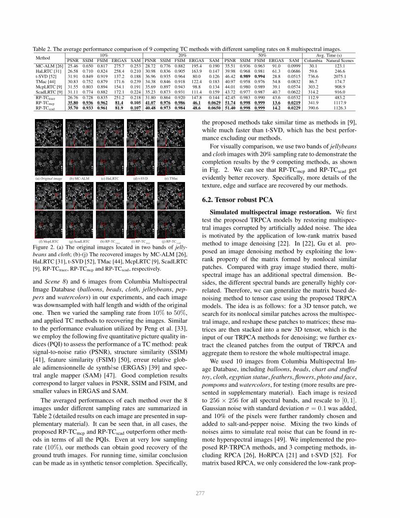
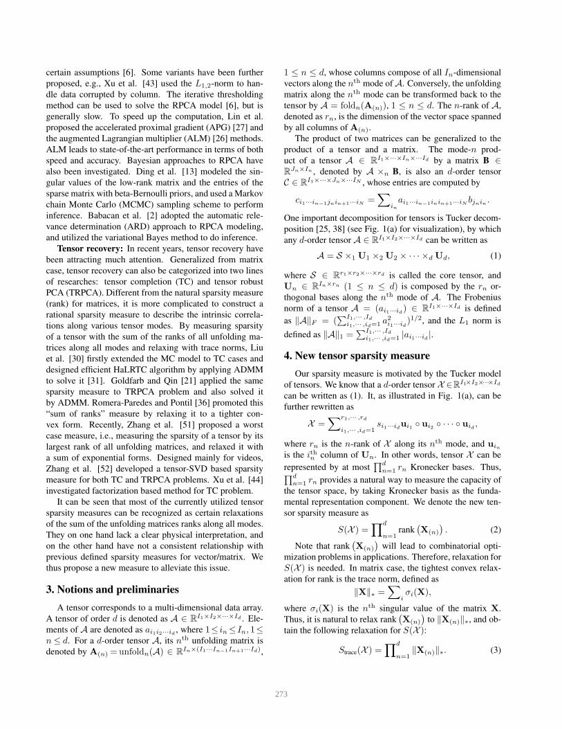
Table 2. The average performance comparison of 9 competing TC methods with different sampling rates on 8 multispectral images.

Method10% 20% 50% Avg. Time (s)

PSNR SSIM FSIM ERGAS SAM PSNR SSIM FSIM ERGAS SAM PSNR SSIM FSIM ERGAS SAM Columbia Natural Scenes

MC-ALM [26] 25.46 0.650 0.817 275.7 0.253 28.72 0.776 0.882 195.4 0.190 35.51 0.936 0.963 91.0 0.0999 30.1 123.1

HaLRTC [31] 26.58 0.710 0.824 258.4 0.210 30.98 0.836 0.905 163.9 0.147 39.98 0.968 0.981 61.3 0.0686 59.6 246.6

t-SVD [52] 31.91 0.849 0.919 137.2 0.188 36.96 0.935 0.964 80.0 0.126 46.42 0.989 0.994 28.8 0.0515 736.6 2075.1

TMac [44] 30.83 0.752 0.879 171.6 0.239 34.38 0.846 0.918 122.4 0.183 40.97 0.958 0.976 54.8 0.0832 86.7 174.7

McpLRTC [9] 31.55 0.803 0.894 154.1 0.191 35.69 0.897 0.943 98.8 0.134 44.01 0.980 0.989 39.1 0.0574 303.2 908.9

ScadLRTC [9] 31.11 0.774 0.882 172.1 0.224 35.23 0.873 0.931 111.4 0.159 43.72 0.977 0.987 40.7 0.0622 314.2 916.0

RP-TCtrace 26.76 0.728 0.835 251.2 0.218 31.80 0.864 0.920 147.8 0.144 42.45 0.983 0.990 43.6 0.0532 112.9 483.2

RP-TCmcp 35.80 0.936 0.962 81.4 0.105 41.07 0.976 0.986 46.1 0.0629 51.74 0.998 0.999 13.6 0.0219 341.9 1117.9

RP-TCscad 35.70 0.933 0.961 81.9 0.107 40.48 0.973 0.984 48.6 0.0650 51.40 0.998 0.999 14.2 0.0229 390.6 1126.3

(a) Original image (b) MC-ALM (c) HaLRTC (d) t-SVD (e) TMac

(h) RP-TCt race

(i) RP-TCmcp

(j) RP-TCscad

(f) McpLRTC (g) ScadLRTC

Figure 2. (a) The original images located in two bands of jelly-

beans and cloth; (b)-(j) The recovered images by MC-ALM [26],

HaLRTC [31], t-SVD [52], TMac [44], McpLRTC [9], ScadLRTC

[9], RP-TCtrace, RP-TCmcp and RP-TCscad, respectively.

and Scene 8) and 6 images from Columbia Multispectral

Image Database (balloons, beads, cloth, jelleybeans, pep-

pers and watercolors) in our experiments, and each image

was downsampled with half length and width of the original

one. Then we varied the sampling rate from 10% to 50%,

and applied TC methods to recovering the images. Similar

to the performance evaluation utilized by Peng et al. [33],

we employ the following five quantitative picture quality in-

dices (PQI) to assess the performance of a TC method: peak

signal-to-noise ratio (PSNR), structure similarity (SSIM)

[41], feature similarity (FSIM) [50], erreur relative glob-

ale adimensionnelle de synthese (ERGAS) [39] and spec-

tral angle mapper (SAM) [47]. Good completion results

correspond to larger values in PSNR, SSIM and FSIM, and

smaller values in ERGAS and SAM.

The averaged performances of each method over the 8

images under different sampling rates are summarized in

Table 2 (detailed results on each image are presented in sup-

plementary material). It can be seen that, in all cases, the

proposed RP-TCmcp and RP-TCscad outperform other meth-

ods in terms of all the PQIs. Even at very low sampling

rate (10%), our methods can obtain good recovery of the

ground truth images. For running time, similar conclusion

can be made as in synthetic tensor completion. Specifically,

the proposed methods take similar time as methods in [9],

while much faster than t-SVD, which has the best perfor-

mance excluding our methods.

For visually comparison, we use two bands of jellybeans

and cloth images with 20% sampling rate to demonstrate the

completion results by the 9 competing methods, as shown

in Fig. 2. We can see that RP-TCmcp and RP-TCscad get

evidently better recovery. Specifically, more details of the

texture, edge and surface are recovered by our methods.

6.2. Tensor robust PCA

Simulated multispectral image restoration. We first

test the proposed TRPCA models by restoring multispec-

tral images corrupted by artificially added noise. The idea

is motivated by the application of low-rank matrix based

method to image denoising [22]. In [22], Gu et al. pro-

posed an image denoising method by exploiting the low-

rank property of the matrix formed by nonlocal similar

patches. Compared with gray image studied there, multi-

spectral image has an additional spectral dimension. Be-

sides, the different spectral bands are generally highly cor-

related. Therefore, we can generalize the matrix based de-

noising method to tensor case using the proposed TRPCA

models. The idea is as follows: for a 3D tensor patch, we

search for its nonlocal similar patches across the multispec-

tral image, and reshape these patches to matrices; these ma-

trices are then stacked into a new 3D tensor, which is the

input of our TRPCA methods for denoising; we further ex-

tract the cleaned patches from the output of TRPCA and

aggregate them to restore the whole multispectral image.

We used 10 images from Columbia Multispectral Im-

age Database, including balloons, beads, chart and stuffed

toy, cloth, egyptian statue, feathers, flowers, photo and face,

pompoms and watercolors, for testing (more results are pre-

sented in supplementary material). Each image is resized

to 256 × 256 for all spectral bands, and rescale to [0, 1].Gaussian noise with standard deviation σ = 0.1 was added,

and 10% of the pixels were further randomly chosen and

added to salt-and-pepper noise. Mixing the two kinds of

noises aims to simulate real noise that can be found in re-

mote hyperspectral images [49]. We implemented the pro-

posed RP-TRPCA methods, and 3 competing methods, in-

cluding RPCA [26], HoRPCA [21] and t-SVD [52]. For

matrix based RPCA, we only considered the low-rank prop-

277

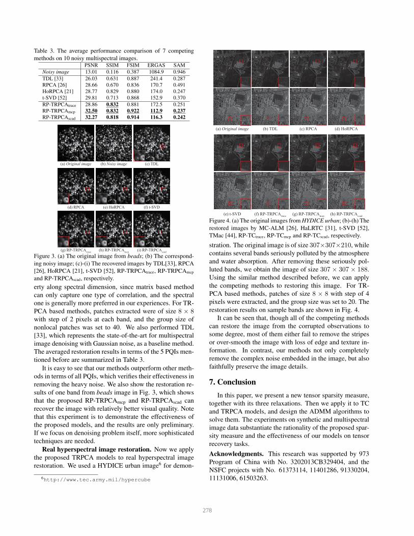
Table 3. The average performance comparison of 7 competing

methods on 10 noisy multispectral images.PSNR SSIM FSIM ERGAS SAM

Noisy image 13.01 0.116 0.387 1084.9 0.946

TDL [33] 26.03 0.631 0.887 241.4 0.287

RPCA [26] 28.66 0.670 0.836 170.7 0.491

HoRPCA [21] 28.77 0.829 0.880 174.0 0.247

t-SVD [52] 29.81 0.713 0.868 152.9 0.370

RP-TRPCAtrace 28.86 0.832 0.881 172.5 0.251

RP-TRPCAmcp 32.50 0.832 0.922 112.9 0.237

RP-TRPCAscad 32.27 0.818 0.914 116.3 0.242

(a) Original image

(d) RPCA

(c) TDL

(e) HoRPCA (f) t-SVD

(i) RP-TRPCAscad

(g) RP-TRPCAt race

(h) RP-TRPCAmcp

(b) Noisy image

Figure 3. (a) The original image from beads; (b) The correspond-

ing noisy image; (c)-(i) The recovered images by TDL[33], RPCA

[26], HoRPCA [21], t-SVD [52], RP-TRPCAtrace, RP-TRPCAmcp

and RP-TRPCAscad, respectively.

erty along spectral dimension, since matrix based method

can only capture one type of correlation, and the spectral

one is generally more preferred in our experiences. For TR-

PCA based methods, patches extracted were of size 8 × 8with step of 2 pixels at each band, and the group size of

nonlocal patches was set to 40. We also performed TDL

[33], which represents the state-of-the-art for multispectral

image denoising with Gaussian noise, as a baseline method.

The averaged restoration results in terms of the 5 PQIs men-

tioned before are summarized in Table 3.

It is easy to see that our methods outperform other meth-

ods in terms of all PQIs, which verifies their effectiveness in

removing the heavy noise. We also show the restoration re-

sults of one band from beads image in Fig. 3, which shows

that the proposed RP-TRPCAmcp and RP-TRPCAscad can

recover the image with relatively better visual quality. Note

that this experiment is to demonstrate the effectiveness of

the proposed models, and the results are only preliminary.

If we focus on denoising problem itself, more sophisticated

techniques are needed.

Real hyperspectral image restoration. Now we apply

the proposed TRPCA models to real hyperspectral image

restoration. We used a HYDICE urban image6 for demon-

6http://www.tec.army.mil/hypercube

(a) Original image (c) RPCA(b) TDL (d) HoRPCA

(e) t-SVD (h) RP-TRPCAscad

(f) RP-TRPCAt race

(g) RP-TRPCAmcp

Figure 4. (a) The original images from HYDICE urban; (b)-(h) The

restored images by MC-ALM [26], HaLRTC [31], t-SVD [52],

TMac [44], RP-TCtrace, RP-TCmcp and RP-TCscad, respectively.

stration. The original image is of size 307×307×210, while

contains several bands seriously polluted by the atmosphere

and water absorption. After removing these seriously pol-

luted bands, we obtain the image of size 307 × 307 × 188.

Using the similar method described before, we can apply

the competing methods to restoring this image. For TR-

PCA based methods, patches of size 8 × 8 with step of 4

pixels were extracted, and the group size was set to 20. The

restoration results on sample bands are shown in Fig. 4.

It can be seen that, though all of the competing methods

can restore the image from the corrupted observations to

some degree, most of them either fail to remove the stripes

or over-smooth the image with loss of edge and texture in-

formation. In contrast, our methods not only completely

remove the complex noise embedded in the image, but also

faithfully preserve the image details.

7. Conclusion

In this paper, we present a new tensor sparsity measure,

together with its three relaxations. Then we apply it to TC

and TRPCA models, and design the ADMM algorithms to

solve them. The experiments on synthetic and multispectral

image data substantiate the rationality of the proposed spar-

sity measure and the effectiveness of our models on tensor

recovery tasks.

Acknowledgments. This research was supported by 973

Program of China with No. 3202013CB329404, and the

NSFC projects with No. 61373114, 11401286, 91330204,

11131006, 61503263.

278

References

[1] E. Acar, D. M. Dunlavy, T. G. Kolda, and M. Mørup. Scalable tensor fac-torizations for incomplete data. Chemometrics and Intelligent Laboratory

Systems, 106(1):41–56, 2001.

[2] S. D. Babacan, M. Luessi, R. Molina, and A. K. Katsaggelos.Sparse Bayesian methods for low-rank matrix estimation. IEEE TSP,60(8):3964–3977, 2012.

[3] S. Boyd, N. Parikh, E. Chu, B. Peleato, and J. Eckstein. Distributed op-timization and statistical learning via the alternating direction method ofmultipliers. Foundations and Trends in Machine Learning, 3(1):1–122,2011.

[4] J. F. Cai, E. J. Candes, and Z. Shen. A singular value thresholding algo-rithm for matrix completion. SIAM Journal on Optimization, 20(4):1956–1982, 2010.

[5] C. F. Caiafa and A. Cichocki. Computing sparse representations ofmultidimensional signals using Kronecker bases. Neural Computation,25(1):186–220, 2013.

[6] E. J. Candes, X. Li, Y. Ma, and J. Wright. Robust principal componentanalysis? Journal of the ACM, 58(3):11:1–11:37, 2011.

[7] E. J. Candes and B. Recht. Exact matrix completion via convex optimiza-tion. Foundations of Computational Mathematics, 9(6):717–772, 2009.

[8] E. J. Candes, J. Romberg, and T. Tao. Stable signal recovery from in-complete and inaccurate measurements. Communications on Pure and

Applied Mathematics, 59(8):1207–1223, 2006.

[9] W. Cao, Y. Wang, C. Yang, X. Chang, Z. Han, and Z. Xu. Folded-concave penalization approaches to tensor completion. Neurocomputing,152(0):261 – 273, 2015.

[10] V. Chandrasekaran, B. Recht, P. A. Parrilo, and A. S. Willsky. The convexalgebraic geometry of linear inverse problems. Foundations of Computa-

tional Mathematics, 12(6):805–849, 2012.

[11] R. Chartrand. Exact reconstruction of sparse signals via nonconvex mini-mization. IEEE Signal Processing Letters, 14(10):707–710, 2007.

[12] Y. L. Chen, C.-T. Hsu, and H.-Y. M. Liao. Simultaneous tensor decompo-sition and completion using factor priors. IEEE TPAMI, 36(3):577–591,2014.

[13] X. Ding, L. He, and L. Carin. Bayesian robust principal component anal-ysis. IEEE TIP, 20(12):3419–3430, 2011.

[14] D. Donoho. Compressed sensing. IEEE TIT, 52(4):1289–1306, 2006.

[15] C. Eckart and G. Young. The approximation of one matrix by another oflower rank. Psychometrika, 1(3):211–218, 1936.

[16] J. Fan and R. Li. Variable selection via nonconcave penalized likelihoodand its oracle properties. Journal of the American Statistical Association,96(456):1348–1360, 2001.

[17] J. Fan, L. Xue, and H. Zou. Strong oracle optimality of folded concavepenalized estimation. Annals of Statistics, 42(3):819–849, 2014.

[18] Z. Y. Feng, S. H. Feng, R. Jin, and A. K. Jain. Image tag completion bynoisy matrix recovery. In ECCV, 2014.

[19] D. H. Foster, K. Amano, S. Nascimento, and M. J. Foster. Frequency ofmetamerism in natural scenes. Journal of the Optical Society of America

A, 23(10):2359–2372, 2006.

[20] S. Gandy, B. Recht, and I. Yamada. Tensor completion and low-n ranktensor recovery via convex optimization. Inverse Problems, 27(3):331–336, 2011.

[21] D. Goldfarb and Z. T. Qin. Robust low-rank tensor recovery: Mod-els and algorithms. SIAM Journal on Matrix Analysis and Applications,35(1):225–253, 2014.

[22] S. Gu, L. Zhang, W. Zuo, and X. Feng. Weighted nuclear norm minimiza-tion with application to image denoising. In CVPR, 2014.

[23] Y. Hu, D. B. Zhang, J. P. Ye, X. L. Li, and X. F. He. Fast and accurate ma-trix completion via truncated nuclear norm regularization. IEEE TPAMI,35(9):2117–2130, 2013.

[24] T. G. Kolda and B. W. Bader. Tensor decompositions and applications.SIAM Review, 51(3):455–500, 2009.

[25] L. D. Lathauwer, B. D. Moor, and J. Vandewalle. A multilinear singularvalue decomposition. SIAM Journal on Matrix Analysis and Applications,21(4):1253–1278, 2000.

[26] Z. Lin, M. Chen, and Y. Ma. The augmented Lagrange multiplier methodfor exact recovery of corrupted low-rank matrices. Technical ReportUILU-ENG-09-2215, UIUC, 2009.

[27] Z. Lin, A. Ganesh, J. Wright, L. Wu, M. Chen, and Y. Ma. Fast convex op-timization algorithms for exact recovery of a corrupted low-rank matrix.Technical Report UILU-ENG-09-2214, UIUC, 2009.

[28] Z. C. Lin, R. S. Liu, and Z. X. Su. Linearized alternating direction methodwith adaptive penalty for low rank representation. In NIPS, 2011.

[29] D. Liu, T. Zhou, H. Qian, C. Xu, and Z. Zhang. A nearly unbiased matrixcompletion approach. In ECML/PKDD, 2013.

[30] J. Liu, P. Musialski, P. Wonka, and J. P. Ye. Tensor completion for esti-mating missing values in visual data. In ICCV, 2009.

[31] J. Liu, P. Musialski, P. Wonka, and J. P. Ye. Tensor completion for esti-mating missing values in visual data. IEEE TPAMI, 34(1):208–220, 2013.

[32] S. Lu, X. F. Ren, and F. Liu. Depth enhancement via low-rank matrixcompletion. In CVPR, 2014.

[33] Y. Peng, D. Y. Meng, Z. B. Xu, C. Q. Gao, Y. Yang, and B. Zhang. De-composable nonlocal tensor dictionary learning for multispectral imagedenoising. In CVPR, 2014.

[34] B. Recht, M. Fazel, and P. A. Parrilo. Guaranteed minimum-rank solu-tions of linear matrix equations via nuclear norm minimization. SIAM

Review, 52(3):471–501, 2010.

[35] J. D. M. Rennie and N. Srebro. Fast maximum margin matrix factorizationfor collaborative prediction. In ICML, 2005.

[36] B. Romera-Paredes and M. Pontil. A new convex relaxation for tensorcompletion. In NIPS, 2013.

[37] M. Signoretto, R. V. de Plas, B. D. Moor, and J. A. K. Suykens. Tensorversus matrix completion: A comparison with application to spectral data.IEEE Signal Processing Letters, 18(7):403–406, 2011.

[38] L. R. Tucker. Some mathematical notes on three-mode factor analysis.Psychometrika, 31(3):279–311, 1966.

[39] L. Wald. Data Fusion: Definitions and Architectures: Fusion of Images

of Different Spatial Resolutions. Presses de l’Ecole des Mines, 2002.

[40] S. Wang, D. Liu, and Z. Zhang. Nonconvex relaxation approaches torobust matrix recovery. In IJCAI, 2013.

[41] Z. Wang, A. C. Bovik, H. R. Sheikh, and E. P. Simoncelli. Image qual-ity assessment: from error visibility to structural similarity. IEEE TIP,13(4):600–612, 2004.

[42] J. Wright, Y. Peng, Y. Ma, A. Ganesh, and S. Rao. Robust principalcomponent analysis: Exact recovery of corrupted low-rank matrices byconvex optimization. In NIPS, 2009.

[43] H. Xu, C. Caramanis, and S. Sanghavi. Robust PCA via outlier pursuit.In NIPS, 2010.

[44] Y. Xu, R. Hao, W. Yin, and Z. Su. Parallel matrix factorization for low-rank tensor completion. arXiv preprint arXiv:1312.1254, 2013.

[45] Z. Xu, X. Chang, F. Xu, and H. Zhang. L1/2 regularization: A thresh-olding representation theory and a fast solver. IEEE TNNLS, 23(7):1013–1027, 2012.

[46] F. Yasuma, T. Mitsunaga, and D. Iso. Generalized assorted pixel camera:postcapture control of resolution, dynamic range and spectrum. IEEE TIP,19(9):2241–2253, 2010.

[47] R. H. Yuhas, J. W. Boardman, and A. F. H. Goetz. Determination of semi-arid landscape endmembers and seasonal trends using convex geometryspectral unmixing techniques. In Summaries of the 4th Annual JPL Air-

borne Geoscience Workshop, 1993.

[48] C. Zhang. Nearly unbiased variable selection under minimax concavepenalty. Annals of Statistics, 38(2):894–942, 2010.

[49] H. Zhang, W. He, L. Zhang, H. Shen, and Q. Yuan. Hyperspectral imagerestoration using low-rank matrix recovery. IEEE TGRS, 52(8):4729–4743, Aug 2014.

[50] L. Zhang, X. Q. Mou, and D. Zhang. Fsim: a feature similarity index forimage quality assessment. IEEE TIP, 20(8):2378C–2386, 2011.

[51] X. Q. Zhang, Z. Y. Zhou, D. Wang, and Y. Ma. Hybrid singular valuethresholding for tensor completion. In AAAI, 2014.

[52] Z. M. Zhang, G. Ely, S. Aeron, N. Hao, and M. E. Kilmer. Novel methodsfor multilinear data completion and de-noising based on tensor-SVD. InCVPR, 2014.

279