1

Abstract—The aim of this paper is to detail the development of

a novel tracking framework that is able to extract the cell

motility indicators and to determine the cellular division (mitosis)

events in large time-lapse phase-contrast image sequences. To

address the challenges induced by non-structured (random)

motion, cellular agglomeration, and cellular mitosis, the process

of automatic (unsupervised) cell tracking is carried out in a

sequential manner, where the inter-frame cell association is

achieved by assessing the variation in the local cellular structures

in consecutive frames of the image sequence. In our study a

strong emphasis has been placed on the robust use of the

topological information in the cellular tracking process and in the

development of targeted pattern recognition techniques that were

designed to redress the problems caused by segmentation errors,

and to precisely identify mitosis using a backward (reversed)

tracking strategy. The proposed algorithm has been evaluated on

dense phase contrast cellular data and the experimental results

indicate that the proposed algorithm is able to accurately track

epithelial and endothelial cells in time-lapse image sequences that

are characterized by low contrast and high level of noise. Our

algorithm achieved 86.10% overall tracking accuracy and

90.12% mitosis detection accuracy.

Index Terms— Cell tracking, Delaunay triangulation, cellular

interaction, mitosis, time-lapse microscopy.

I. INTRODUCTION

ELL migration is one of the key cellular processes that is

associated with a wide range of biological phenomena

including embryogenesis, inflammation, wound healing,

tumour development [1], [2], and its accurate estimation plays

an important role in cell and molecular biology research [3].

Typically, cell migration is evaluated in time-lapse image data

and the current practice involves a labour intensive (manual)

procedure that is applied to analyze/track the cells in all

frames of the image sequence. With the advent of modern

microscopy imaging modalities the amount of information

required to be analyzed by clinical experts has substantially

increased and in many situations the standard manual

This work was supported by the National Bio-photonics and Imaging

Platform (NBIP) Ireland funded under the Higher Education Authority PRTLI

Cycle 4, co-funded by the Irish Government and the European Union - /Investing in your future/.

K. Thirusittampalam is with the Center for Image Processing and Analysis,

Dublin City University, Ireland. (phone: 353-1-700-7636; fax: 353-1-700-

5508; e-mail: thirusittampalm.ketheesan2@mail.dcu.ie).

M. J. Hossain, O. Ghita, and P. F. Whelan are with the Center for Image

Processing and Analysis, Dublin City University, Ireland. (e-mail: julius.hossain@dcu.ie, ghitao@eeng.dcu.ie, and paul.whelan@dcu.ie).

procedure has become impractical [2]. The limitations of the

manual procedures when applied to the estimation of cell

migration opened a new research area that addresses the

development of computer vision–based automatic cellular

tracking algorithms.

Automatic cellular tracking is challenging due to several

factors such as low image contrast, changes in the morphology

of the cells over time, random migration, cell division [19],

[27], [28], cell interaction [7] and low signal to noise ratio.

These challenges vary to a great extent depending on the

characteristics of the imaging systems or on the nature of the

cell lines being analyzed, and as a result numerous semi-

automatic [4]-[6] and fully automatic [1], [8], [11] cell

tracking algorithms were proposed in the literature. When the

published algorithms are evaluated from a computer vision

standpoint, two main categories can be identified. Thus, the

first category of cell tracking algorithms includes

segmentation-driven approaches [1], [4], [7]-[9], [20], [30],

[31], while the second category comprises model-based

approaches that typically are either based on contour

propagation [5], [11]-[17] or on the combination between

intensity/shape models and motion prediction (using Kalman

and particle filtering) [10], [17], [18]. Among these two

categories, the segmentation-driven cell tracking strategies

proved more successful when applied to phase-contrast

cellular data [26], [29] due to their improved resilience to

variations in imaging conditions, high cell density, cellular

agglomeration, cellular division and sudden changes in cell

morphology. During the development of cell tracking

techniques for phase-contrast cellular-data, the main issues are

associated with the avoidance of cell segmentation errors and

the implementation of robust association rules that are able to

enforce the continuity of the tracking process in the spatio-

temporal domain in the presence of cellular division.

In this context, the major objective of this paper is to

describe the implementation of a fully automatic cell tracking

framework that has been specifically designed to address the

identification of the cell lineages and detect mitosis in dense

time-lapse phase-contrast cellular data. In the proposed

framework, the cells are segmented in each frame using a

multi-phase adaptive algorithm and the cell association

process is carried out by evaluating the topology of the local

cell structures in consecutive frames of the sequence. In our

implementation the connectivity rules between neighbouring

cells are encoded using Delaunay triangulation [21]. Since the

A Novel Framework for Cellular Tracking and

Mitosis Detection in Dense Phase Contrast

Microscopy Images

Ketheesan Thirusittmapalam, M. Julius Hossain, Member, IEEE, Ovidiu Ghita, and Paul F. Whelan,

Senior Member, IEEE

C

2

Segmentation

Centroid

detection

Inter-frame cell

association

Construct the

Delaunay mesh

in each frame

Under-segmentation

module

Cell association

complete?

Image sequence

CS

New track

identified?

Determine

missing cell location

Mitosis

identified?

Output

FWT

No

Yes

Yes

No Yes No

BWT

Start analyzing the FWT results in a backward manner to identify

the mitosis (cell divisions) events

Link the child cell

to the parent cell

phase-contrast cellular data that is evaluated in this study is

characterized by large contrast variation and a relative high

level of noise, the identification of the cells throughout the

sequence proved quite difficult. To compensate for the

segmentation errors we have developed a novel approach

based on the evaluation of the alterations in the local cellular

structures which proved capable of detecting and correcting

the errors caused by under-segmentation, with sizeable

improvements in relation to tracking accuracy. The last

component of the proposed algorithm addresses the mitosis

detection using a hybrid implementation that combines the

backward tracking analysis with the application of normalized

cross correlation for the identification of the child cells that

were missed by the forward tracking phase of the algorithm.

The experimental tests have been performed using in-vitro

time-lapse phase contrast image sequences. While the major

contributions that emerge from our work are associated with

the proposed computational framework that has been designed

to address cellular tracking and mitosis detection, we would

like to mention that another important contribution is given by

the detailed evaluation of our algorithm when applied to

various cell-specific data and in the comparative analysis that

investigates the performances obtained by our framework and

other related cell tracking algorithms.

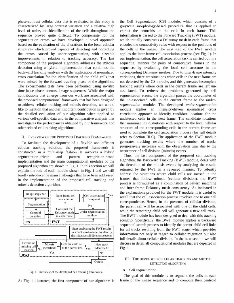
II. OVERVIEW OF THE PROPOSED TRACKING FRAMEWORK

To facilitate the development of a flexible and efficient

cellular tracking solution, the proposed framework is

constructed in a multi-step fashion. It involves a hybrid

segmentation-driven and pattern recognition-based

implementation and the main computational modules of the

proposed algorithm are shown in Fig. 1. In this section we will

explain the role of each module shown in Fig. 1 and we will

briefly introduce the main challenges that have been addressed

in the implementation of the proposed cell tracking and

mitosis detection algorithm.

Fig. 1. Overview of the developed cell tracking framework.

As Fig. 1 illustrates, the first component of our algorithm is

the Cell Segmentation (CS) module, which consists of a

greyscale morphology-based procedure that is applied to

extract the centroids of the cells in each frame. This

information is passed to the Forward Tracking (FWT) module,

which initially constructs a Delaunay mesh in each frame that

encodes the connectivity rules with respect to the positions of

the cells in the image. The next step of the FWT module

applies the inter-frame cell association process (see Fig. 1). In

our implementation, the cell association task is carried out in a

sequential manner for pairs of consecutive frames in the

sequence, by evaluating the local cell structure in the

corresponding Delaunay meshes. Due to inter-frame intensity

variations, there are situations when cells in the next frame are

not detected by the CS module, and this generates incomplete

tracking results where cells in the current frame are left un-

associated. To redress the problems generated by cell

segmentation errors, the algorithm passes the coordinates of

the un-associated cells in the current frame to the under-

segmentation module. The developed under-segmentation

module applies an intensity-driven normalized cross

correlation approach to identify candidate locations for the

undetected cells in the next frame. The candidate locations

that minimize the distortions with respect to the local cellular

structure of the corresponding cells in the current frame are

used to complete the cell association process (for full details

refer to Section III.C). The application of the FWT module

generates tracking results where the number of tracks

progressively increases with the observation time due to the

occurrence of cell division (mitosis) events.

Thus, the last component of the proposed cell tracking

algorithm, the Backward Tracking (BWT) module, deals with

the detection of the mitosis events by analysing the results

returned by the FWT in a reversed manner. To robustly

address the situations where child cells are missed in the

frames that follow mitosis (cellular division), the BWT

process is formulated as a combination of pattern matching

and inter-frame Delaunay mesh consistency. As indicated in

the explanations provided for the FWT module, it is useful to

recall that the cell association process involves one to one cell

correspondence. Hence, in the presence of cellular division,

the parent cell will be associated with one of the child cells,

while the remaining child cell will generate a new cell track.

The BWT module has been designed to deal with this tracking

scenario. Specifically, the BWT module applies a backward

sequential search process to identify the parent-child cell links

for all tracks resulting from the FWT stage, which provides

information not only in regard to cellular migration but also

full details about cellular division. In the next section we will

discuss in detail all computational modules that are depicted in

Fig. 1.

III. THE DEVELOPED CELLULAR TRACKING AND MITOSIS

DETECTION ALGORITHM

A. Cell segmentation

The goal of this module is to segment the cells in each

frame of the image sequence and to compute their centroid

3

points that are required to construct the Delaunay mesh. In

phase contrast data, the image areas covered by cells have

generally a darker interior (nuclei) which is surrounded by a

peripheral bright halo [5]. Following this intensity profile

model, the cells can be theoretically extracted using threshold-

based segmentation techniques. However, our experiments

clearly indicated that the application of simplistic thresholding

schemes does not provide a robust segmentation option, as the

contrast between the cells and background is not constant

within the same image and in addition the distribution of the

intensity values within the cells areas shows a large degree of

variation. Moreover, substantial intensity offsets can be

present when the cell data is analyzed in different frames of

the sequence, and this issue inserts an additional challenge that

has to be addressed by the cell segmentation algorithm. To

provide an insight into this problem, Fig. 2(a) shows a section

cropped from a phase contrast image containing Madin-Darby

Canine Kidney (MDCK) epithelial cells. In Fig. 2(a) it can be

observed that the contrast between the cells and background is

shallow and this fact is further emphasized in Fig. 2(b) where

the corresponding histogram is displayed. To factor in the

complications outlined in Fig. 2(b), we have developed a cell

segmentation scheme that is able to accommodate the shifts in

the intensity domain and to maximally exploit the contrast

difference between the cells and the background information.

In this regard, the cell regions are highlighted by generating

intensity peaks around the cells’ nuclei by applying a method

that is primarily based on the extended maxima transform

[22].

Fig. 2. The process of cell segmentation. (a) An image section taken from a phase contrast image. (b) Histogram of the image section shown in (a). (c) ITH

- top-hat transformed image. (d) 3D plot of the intensity map for ITH. (e)

Gaussian smoothed data - Iσ. (f) 3D plot of the intensity map for Iσ. (g) Segmentation results using a standard adaptive threshold approach [23]. (h)

Segmentation result obtained by the proposed method. (i) The borders and the

centroids of the segmented cells (for clarity purposes they are overlaid on the input image).

The proposed cell segmentation scheme consists of several

steps. Initially, the top-hat transform is applied to enhance the

local contrast, reduce the background noise and the uneven

illumination: ITH = tophat(Ī,S(r)) = Ī – ( Ī o S(r)), where Ī is the

inverted input image, ITH is the top-hat transformed image and

S(r) is a circular structuring element. The radius r is

experimentally determined using the constraint that the

structuring element should be larger than the cell nuclei. This

condition ensures that all cellular structures that are present in

the image are preserved. The output of the top-hat transform

when applied to the image data shown in Fig. 2(a) is depicted

in Fig. 2(c). As illustrated in Fig. 2(d) the application of the

top-hat transform increases the contrast between the cell

nuclei and the background, but it can be observed that some

noisy peaks are still present in the top-hat transformed image

(ITH). This image also details situations where several local

peaks are located inside the area covered by a single cell. To

remove these problems, the data resulting from the top-hat

transform is smoothed using a Gaussian filter and the result is

shown in Fig. 2(e). In our implementation, to efficiently

suppress the noisy peaks inside the cell, we set the scale σ of

the Gaussian filter to r. To illustrate the inappropriateness of

the standard thresholding approaches when applied to the

segmentation of phase contrast cellular data, the adaptive

scheme detailed in [23] has been applied to the Gaussian

smoothed image, Iσ, and the result is shown in Fig. 2(g). Fig.

2(g) indicates that the application of the adaptive thresholding

method generates a binary data where only one blob was

identified. This result clearly highlights the limitations of the

threshold-based methods when applied to dense cellular data

where the transitions between the cells’ nuclei and the

background are very shallow. In our approach, to detect the

cells’ nuclei we applied the extended maxima transform,

which is the regional maxima of the h-maxima transform - the

value of h is experimentally determined (in our studies the

segmentation algorithm has shown good stability when the

value of the parameter h has been set in the interval [10, 19] -

for more details in regard to the selection of the parameter h

refer to Table 1, Section IV). Fig. 2(h) shows the result

obtained after the application of the extended maxima

transform which provides an accurate segmentation of the

cells’ nuclei. For clarity purposes, in Fig. 2(i) the cells borders

(marked in green) and their centroids (marked in red) are

overlaid on the input image.

Additional results that illustrate the performance of the

developed morphological-based cell segmentation algorithm

in the presence of cellular agglomeration are presented in Fig.

3. The next subsection presents a pseudo-code sequence where

the main steps of the proposed cell tracking and mitosis

algorithm are outlined.

b a c

d e f

g i h

4

a b

Fig. 3. Cell segmentation results in the presence of cell agglomeration. (a) Image sections cropped from three MDCK datasets. (b) Cell segmentation

results. For visualisation purposes, cellular agglomeration cases are marked

with black ellipses in images shown in column (a) and the borders and centroids of the segmented cells are overlaid on the results shown in column

(b) with green contours and red dots, respectively.

Pseudo-code detailing the main steps of the proposed cellular

tracking and mitosis detection algorithm

A. Apply cell segmentation to all frames of the sequence.

Forward Tracking steps

B. Forward tracking (FWT) cell association (frames T and T+1)

B1. Construct Delaunay meshes in frames T and T+1 B2. Evaluate the local structure (triangle) matching using equation (4)

B3. Associate cells that have their local structures completely matched

B4. Generate the reference nodes list R B5. Associate cells for which MC(.)<1 (cells with local structures partially

matched) using equation (8) and add them to the list R

B6. For each unassociated cell in image T (due to under-segmentation) B6.1. Find the corresponding location for each unassociated cell in

frame T by applying normalized cross correlation and the use of

local structure in frame T+1 (activation of under-segmentation module).

Repeat steps B1 to B6 until the last image in the sequence is processed and

generate the forward tracking (FWT) results.

Backward Tracking steps

C. Mitosis detection – perform backward tracking for all tracks TKi

identified by FWT

C1. Identify the first frame (frame T) associated with the track TKi (frame

in which the cell that generated the track TKi was detected first)

If: frame T-1 is the first frame of the sequence: End the analysis for track TKi (the track is complete from first to last frame of the

sequence)

Else: Go to step C2 C2. Apply backward cell association from image T to image T-1

C3. If: no suitable parent cell is identified in frame T-1: activate the under-

segmentation module to determine the location of the undetected cell in frame T-1

C3.1 Repeat step C3 in frames T-2, T-3, etc. until the parent cell is

identified

Else: Parent cell identified in frame T-1

Repeat steps C1 to C3 until all TKi tracks identified by FWT are processed.

Full details for FWT and BWT modules are provided in

Sections III.B and III.C, respectively.

B. Forward tracking module (FWT)

The cell association in dense phase-contrast cellular data

represents a challenging task since cells have similar intensity

and shape characteristics and the cell migration is defined by

random motility patterns. Thus, a cell tracking framework that

implements the association process using feature-matching or

relies on the information supplied by model-based motion

estimators is likely to return inaccurate results. To circumvent

the issues relating to feature ambiguity or inconsistent motion

estimation, the proposed tracking framework evaluates the

structural (topological) relationships among neighbouring cells

in the inter-frame cell association process. To provide a

compact representation that encompasses the spatial

arrangement between neighbouring cells, we employed

Delaunay triangulation to generate a unique planar graph that

is independent on the topology of the nodes [21], [24]. In our

algorithm we have used Delaunay triangulation since this

graph-based representation maximizes the minimum angles of

the triangles that generate the mesh. In this representation the

triangles tend towards equiangularity and the insertion or

removal of a node affects the mesh representation only at the

local level. This property is particularly appropriate to encode

the neighbouring relationship between cells in the image, as

the insertion and the removal of nodes can be caused by

cellular division or under-segmentation. In the proposed

algorithm each node of the mesh represents a cell position that

is given by its centroid, and the edges constructed for each

node during triangulation define the spatial relationship

between the analyzed cell and the cells situated in its close

neighbourhood. Using this representation, the node (cell)

association process can be efficiently formulated as a graph

matching problem, where the local structures associated with

the nodes in the Delaunay mesh are analyzed in consecutive

frames of the image sequence. Since the local inter-cell

relationships are accurately modelled in this formulation, the

similarity between the local Delaunay structures in two

consecutive frames can be efficiently estimated based on the

assumption that cells can be accurately detected in each frame.

However, as indicated in Section III.A, when dealing with

dense phase-contrast data there are situations when cells are

missed by the segmentation process and this generates

substantial changes in the local structure that is encoded by the

Delaunay mesh. While the cellular association process

proposed in our paper is based on the evaluation of the local

structure, missing cells in one frame will have a negative

effect on the accuracy of the tracking process. This is obvious

as the cellular association entails a sequential process, and the

incidence of under-segmentation creates discontinuities in the

cell lineages that are determined for each individual cell. To

overcome this problem, in our implementation we have

developed a procedure (referred to as under-segmentation

module) which determines the location of the missed cell

using an intensity-based pattern matching strategy.

5

Cell association

The correspondence between the cells in frames T and T+1

of the image sequence is determined based on the local

structure associated with the cells in their neighbourhood

graphs DT and D

T+1, respectively, that are obtained using

Delaunay triangulation, as explained in Section III.B. If we

consider a node (cell centroid) u from mesh DT, then the local

structure associated with u is defined as follows:

, , , ,T TuS upq p q D p q p u q u (1)

where p q is a topology operator that denotes that the node

with the index p is adjacent to the node with the index q, Δupq defines the triangular structure that is generated by the u, p, q

nodes and {.} is the mathematical set operator. To aid the

understanding of the mathematical formalism detailed in (1),

Fig. 4 depicts a section of the Delaunay mesh that is

constructed using the centroids of the cells detected in image

T. In this diagram, the local structure associated with the node

u is , , , , ,TuS uab ubc ucd ude uef ufa .

Fig. 4. A section of the Delaunay mesh that illustrates the construction of the

local structure Tus for the node with the index u.

Now, let 1Tvs be the local structure associated with the node

1Tv D in the Delaunay mesh that is constructed using the

detected centroids in frame T+1. At this point we need to

define a metric that is able to sample the similarity in the local

structures that are associated with the two nodes Tu D and 1Tv D . To achieve this goal, we propose to evaluate the

structural similarity between TuS

and 1T

vS in terms of the

similarity among the triangles and the edges that are

associated with the nodes u and v in frames T and T+1,

respectively. Thus, the similarity between two triangles is

defined according to the Hausdorff distance, which records the

largest of all the displacements between one node in one

triangle to the closest node in the other triangle. If Δ1 and Δ2

represent two triangles, then the Hausdorff distance between

these triangles is defined as follows:

1 2 1 2 2 1, max , , ,H (2)

where 1 221

, max min ,qp

d p q

, and ,d p q is the Euclidean

distance between the two nodes with indexes p and q. With

respect to (2), the triangles Δ1 and Δ2 are assumed to be

similar only if their Hausdorff distance is smaller than a

predefined threshold α as illustrated in (3) (a perfect match

between Δ1 and Δ2 is achieved when the Hausdorff distance

H(Δ1,Δ2)=0, i.e. when the corresponding nodes of Δ1 and Δ2

have the same coordinates in frames T and T+1. An increase in

the value of H(Δ1,Δ2) indicates more dissimilarity between Δ1

and Δ2). Since changes in the local structures that are

associated with corresponding nodes in frames T and T+1 are

caused by cell migration, in our implementation the similarity

between two triangles MT(Δ1,Δ2) is evaluated in conjunction

with a parameter α, which is set as the maximum

instantaneous cell movement in two consecutive frames.

1 2

1 2

1, ,,

0,

HMT

otherwise

(3)

As indicated in (1), the local structure associated with each

node consists of a set of triangles that are generated by the

node of interest and the adjacent nodes in the Delaunay mesh.

Thus, to completely evaluate the similarity between the nodes Tu D and 1Tv D , we introduce a matching confidence function

MC(.) that evaluates the similarity between two local

structures TuS and 1T

vS , where the similarity between two

triangles is evaluated using (3).

1,

1

,

,max ,

i jT TS Si u j v

T Tu v

MT

MC u vS S

(4)

where TuS represents the number of triangles contained in the

set TuS . In (4) the numerator evaluates the similarity between

the two sets of triangles contained in the local structures TuS and

1TvS , while the denominator is applied to normalize the

matching confidence, MC(.) values, in the range [0,1]. With

respect to the value of the matching confidence returned for

each pair of nodes (cells) in frames T and T+1, the cells are

associated in multiple stages. In the first stage the nodes (cells)

in frames T and T+1 that have complete structure similarity

(i.e. MT(.) =1 for all triangles in the local structures TuS and

1TvS ) are associated. This situation is illustrated in Figs. 5(a)

and 5(b) where two nodes Tu D and 1Tv D have their

structures completely matched. All nodes Tp D and 1Tq D

that have their local structures completely matched (i.e. are

associated in the first stage) are included in a reference list R

as follows:

1, ,T TR p q p D q D (5)

where p and q form a matched pair.

Fig. 5. Example showing two nodes u and v in frames T (a) and T+1 (b) that

have their local structures Tus ={Δuba, Δuae, Δued, Δudc, Δucb} and 1T

vs ={Δvgf,

Δvfj, Δvji, Δvih, Δvhg} completely matched using (4) and included in the list R.

a

b

c d

e

f u

f

g

h

i

j

v a b

a

b

c

d

e

u

6

The nodes included in the list R are the nodes (cells) that are

associated with the highest confidence and they will be used in

the following stages of the cell association process - when we

attempt to associate the nodes for which the local structure

was only partially matched. In the second step, for nodes with

MC(.) < 1 that have in their local structure at least a pair of

matched nodes included in the list R, we calculate the partial

matching confidence PMC(.), using (8), that evaluates both the

similarity for triangles and mesh edges with respect to the

reference nodes containing in the list R. In this node

association stage we also evaluate the distance between the

nodes to place a higher degree of confidence when matching

the nodes with MC(.) < 1. The last term in (8) penalises the

large displacements of the node v in frame T+1 with respect to

the position of the node u in frame T. The reference edge

structure associated with Tu D is defined as:

,TuE up p R p u (6)

Similarly, the reference edge structure associated with 1Tv D

is defined as:

1 ,TvE vq q R q v (7)

The PMC(.) is calculated as follows:

1

1

, ,, , 1

max E , E

T Tu v

T Tu u

ME E E d u vPMC u v MC u v

(8)

where 1,T Tu vME E E represents the number of matched edges

between TuE and 1T

vE , and TuE denotes the number of edges

in the set TuE . The nodes that maximize the value of PMC(.)

are associated and they are included in the list R.

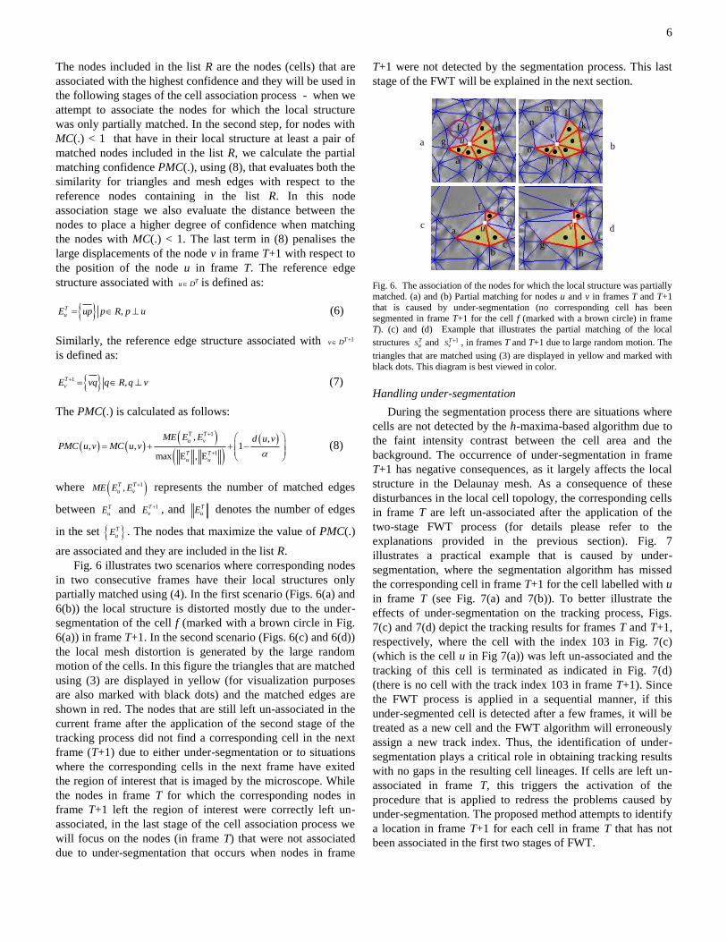
Fig. 6 illustrates two scenarios where corresponding nodes

in two consecutive frames have their local structures only

partially matched using (4). In the first scenario (Figs. 6(a) and

6(b)) the local structure is distorted mostly due to the under-

segmentation of the cell f (marked with a brown circle in Fig.

6(a)) in frame T+1. In the second scenario (Figs. 6(c) and 6(d))

the local mesh distortion is generated by the large random

motion of the cells. In this figure the triangles that are matched

using (3) are displayed in yellow (for visualization purposes

are also marked with black dots) and the matched edges are

shown in red. The nodes that are still left un-associated in the

current frame after the application of the second stage of the

tracking process did not find a corresponding cell in the next

frame (T+1) due to either under-segmentation or to situations

where the corresponding cells in the next frame have exited

the region of interest that is imaged by the microscope. While

the nodes in frame T for which the corresponding nodes in

frame T+1 left the region of interest were correctly left un-

associated, in the last stage of the cell association process we

will focus on the nodes (in frame T) that were not associated

due to under-segmentation that occurs when nodes in frame

T+1 were not detected by the segmentation process. This last

stage of the FWT will be explained in the next section.

Fig. 6. The association of the nodes for which the local structure was partially matched. (a) and (b) Partial matching for nodes u and v in frames T and T+1

that is caused by under-segmentation (no corresponding cell has been

segmented in frame T+1 for the cell f (marked with a brown circle) in frame T). (c) and (d) Example that illustrates the partial matching of the local

structures TuS and 1T

vS , in frames T and T+1 due to large random motion. The

triangles that are matched using (3) are displayed in yellow and marked with

black dots. This diagram is best viewed in color.

Handling under-segmentation

During the segmentation process there are situations where

cells are not detected by the h-maxima-based algorithm due to

the faint intensity contrast between the cell area and the

background. The occurrence of under-segmentation in frame

T+1 has negative consequences, as it largely affects the local

structure in the Delaunay mesh. As a consequence of these

disturbances in the local cell topology, the corresponding cells

in frame T are left un-associated after the application of the

two-stage FWT process (for details please refer to the

explanations provided in the previous section). Fig. 7

illustrates a practical example that is caused by under-

segmentation, where the segmentation algorithm has missed

the corresponding cell in frame T+1 for the cell labelled with u

in frame T (see Fig. 7(a) and 7(b)). To better illustrate the

effects of under-segmentation on the tracking process, Figs.

7(c) and 7(d) depict the tracking results for frames T and T+1,

respectively, where the cell with the index 103 in Fig. 7(c)

(which is the cell u in Fig 7(a)) was left un-associated and the

tracking of this cell is terminated as indicated in Fig. 7(d)

(there is no cell with the track index 103 in frame T+1). Since

the FWT process is applied in a sequential manner, if this

under-segmented cell is detected after a few frames, it will be

treated as a new cell and the FWT algorithm will erroneously

assign a new track index. Thus, the identification of under-

segmentation plays a critical role in obtaining tracking results

with no gaps in the resulting cell lineages. If cells are left un-

associated in frame T, this triggers the activation of the

procedure that is applied to redress the problems caused by

under-segmentation. The proposed method attempts to identify

a location in frame T+1 for each cell in frame T that has not

been associated in the first two stages of FWT.

b

d a

b c

d

e

u

f

v

g h

i

j k

l

l

u

a b

c

d

e

f

g

h i

j

k n

o

v

l m

a

c

7

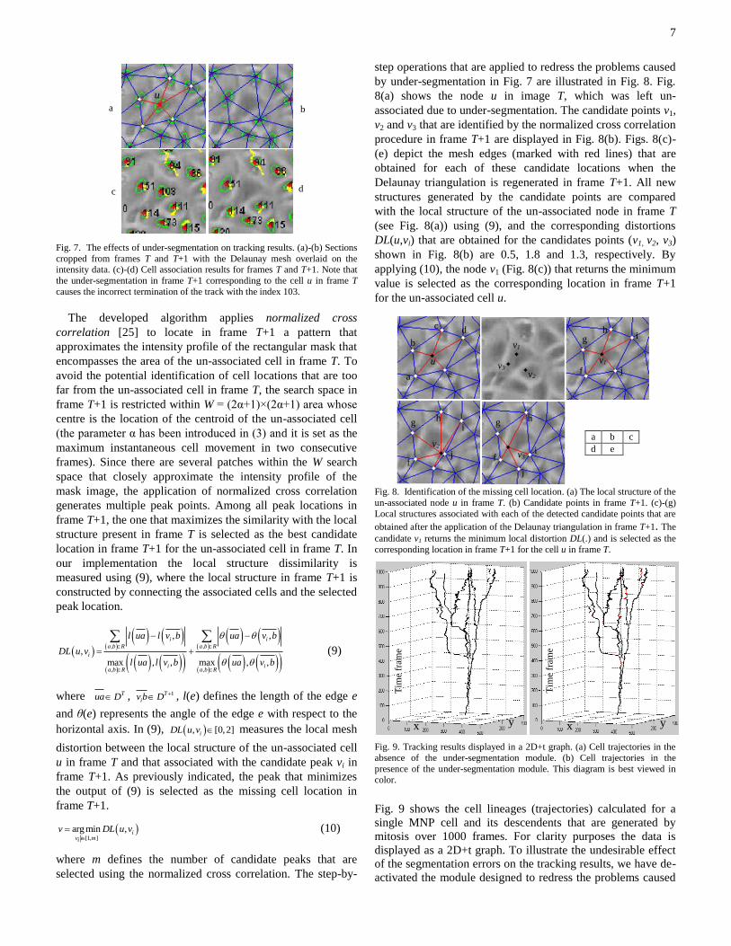
Fig. 7. The effects of under-segmentation on tracking results. (a)-(b) Sections

cropped from frames T and T+1 with the Delaunay mesh overlaid on the intensity data. (c)-(d) Cell association results for frames T and T+1. Note that

the under-segmentation in frame T+1 corresponding to the cell u in frame T

causes the incorrect termination of the track with the index 103.

The developed algorithm applies normalized cross

correlation [25] to locate in frame T+1 a pattern that

approximates the intensity profile of the rectangular mask that

encompasses the area of the un-associated cell in frame T. To

avoid the potential identification of cell locations that are too

far from the un-associated cell in frame T, the search space in

frame T+1 is restricted within W = (2α+1)×(2α+1) area whose

centre is the location of the centroid of the un-associated cell

(the parameter α has been introduced in (3) and it is set as the

maximum instantaneous cell movement in two consecutive

frames). Since there are several patches within the W search

space that closely approximate the intensity profile of the

mask image, the application of normalized cross correlation

generates multiple peak points. Among all peak locations in

frame T+1, the one that maximizes the similarity with the local

structure present in frame T is selected as the best candidate

location in frame T+1 for the un-associated cell in frame T. In

our implementation the local structure dissimilarity is

measured using (9), where the local structure in frame T+1 is

constructed by connecting the associated cells and the selected

peak location.

, ,

, ,

, ,

,

max , , max , ,

i i

a b R a b R

i

i ia b R a b R

l ua l v b ua v b

DL u v

l ua l v b ua v b

(9)

where Tua D , 1Tiv b D , l(e) defines the length of the edge e

and θ(e) represents the angle of the edge e with respect to the

horizontal axis. In (9), , [0,2]iDL u v measures the local mesh

distortion between the local structure of the un-associated cell

u in frame T and that associated with the candidate peak vi in

frame T+1. As previously indicated, the peak that minimizes

the output of (9) is selected as the missing cell location in

frame T+1.

[1, ]

arg min , iv i mi

v DL u v

(10)

where m defines the number of candidate peaks that are

selected using the normalized cross correlation. The step-by-

step operations that are applied to redress the problems caused

by under-segmentation in Fig. 7 are illustrated in Fig. 8. Fig.

8(a) shows the node u in image T, which was left un-

associated due to under-segmentation. The candidate points v1,

v2 and v3 that are identified by the normalized cross correlation

procedure in frame T+1 are displayed in Fig. 8(b). Figs. 8(c)-

(e) depict the mesh edges (marked with red lines) that are

obtained for each of these candidate locations when the

Delaunay triangulation is regenerated in frame T+1. All new

structures generated by the candidate points are compared

with the local structure of the un-associated node in frame T

(see Fig. 8(a)) using (9), and the corresponding distortions

DL(u,vi) that are obtained for the candidates points (v1, v2, v3)

shown in Fig. 8(b) are 0.5, 1.8 and 1.3, respectively. By

applying (10), the node v1 (Fig. 8(c)) that returns the minimum

value is selected as the corresponding location in frame T+1

for the un-associated cell u.

Fig. 8. Identification of the missing cell location. (a) The local structure of the

un-associated node u in frame T. (b) Candidate points in frame T+1. (c)-(g)

Local structures associated with each of the detected candidate points that are

obtained after the application of the Delaunay triangulation in frame T+1. The

candidate v1 returns the minimum local distortion DL(.) and is selected as the

corresponding location in frame T+1 for the cell u in frame T.

Fig. 9. Tracking results displayed in a 2D+t graph. (a) Cell trajectories in the

absence of the under-segmentation module. (b) Cell trajectories in the

presence of the under-segmentation module. This diagram is best viewed in color.

Fig. 9 shows the cell lineages (trajectories) calculated for a

single MNP cell and its descendents that are generated by

mitosis over 1000 frames. For clarity purposes the data is

displayed as a 2D+t graph. To illustrate the undesirable effect

of the segmentation errors on the tracking results, we have de-

activated the module designed to redress the problems caused

a

b

d

e

v1

v2 v3

v1

f

g h

i

j

v2

f

g h

i

v3 f

g h

i

j

j

u

a b c

d e

c

x y

Tim

e fr

ame

x

Tim

e fr

ame

y

u

a b

c d

8

by under-segmentation and the tracking results are depicted in

Fig. 9(a). In Fig. 9(a) it can be clearly observed the significant

number of breaks in the tracking results that are caused by the

segmentation errors. To graphically illustrate the increase in

performance that is induced by the method designed to

compensate for the errors introduced by the segmentation

process, the cell trajectories calculated when the under-

segmentation module is activated are shown in Fig. 9(b). For

illustrative purposes, the tracks that are identified by the

proposed method are marked in red and this diagram

illustrates the significant improvements in terms of tracking

continuity when compared to the results shown in Fig. 9(a). In

Fig. 9(b) the new tracks that are generated by mitosis (cell

division) can also be observed and in the next section we will

detail an algorithm that has been designed to detect mitotic

cells using a backward tracking strategy.

C. Backward tracking module (BWT)

Mitosis is the process by which a parent cell divides into

two similar cells called child or daughter cells. Since the

frequency of the mitosis events plays an important role in

achieving accurate and complete tracking results, in our work

we developed an automatic approach to detect the cell division

using a backward tracking strategy, which links the child

tracks to the corresponding parent cell. Due to intensity

variation and poor contrast in phase contrast image sequences,

child cells are not assured to be detected in all frames. Since

the mitosis events are not a priori known during the forward

tracking process, the parent cell will be linked to one of the

child cells after cell division (i.e. one of the child cells will

have the same track index as the parent cell), while the other

child cell which remains un-associated will generate a track

with a new index. Thus, the detection of mitosis during

forward tracking will be quite problematic, and this is

especially true when dealing with cellular data which does not

exhibit conspicuous intensity transitions in the frame that

precedes cellular division. To robustly detect the mitotic

events, especially when dealing with situations when the child

cell was missed by the segmentation process, we applied a

multi-stage backward tracking process. During backward

tracking, the proposed algorithm determines the location of the

missed child cells (if necessary) and evaluates in a reverse

manner all tracks determined during FWT with the goal of

finding the new tracks that are generated by the cellular

division events. After the application of BWT for each cell in

the dataset, a complete tree structure over the entire image

sequence will be generated, where each branch is associated

with a mitosis event. Fig. 10 illustrates the cell division

process where a parent cell divides in frame T. As indicated

earlier, one of the child cells (child cell-1) is tracked with the

parent ID (TK1) during FWT, while the child cell-2 is detected

by the segmentation module in frame T+2 and will be tracked

in the subsequent frames with a new track index (TK2). As it

can be observed in this diagram, the segmentation algorithm

missed the child cell-2 in frame T+1 and this fact did not

triggered the activation of the under-segmentation procedure

detailed in Section III.B as the parent cell has found a match in

frame T+1 (child cell-1). Thus, this under-segmentation

problem needs to be addressed during backward tracking

(BWT). In this regard, the backward tracking module

approaches the identification of the missing cell location in

frame T+1 starting from frame T+2 in a reversed manner. To

illustrate this process, in Fig. 10 the trajectories analyzed by

the backward tracking are marked with a dashed line. This

process continues with the identification of the missing cell in

frame T. Once the missed cell has been identified (this will be

explained later) in frame T, it can be clearly observed that for

this cell the corresponding cell in frame T-1 is the parent cell

that generated the mitosis event.

Fig. 10. Diagram detailing the cell division process.

Fig. 11. Forward tracking results in the presence of cell division. In this diagram the results of the forward tracking are shown for four consecutive

frames. The child cells resulting from the cellular division are indicated by the

black arrows.

Fig. 11 illustrates the forward tracking results for an image

sequence that sample a cellular division event. In this diagram,

cell-111 shown in frame T divides into two child cells in frame

T+1 where one child cell is tracked with the same index as the

T T-1 T+1 T-2 T+2

Child cell - 1

Track index TK1

Cell

division

T-3 T+3 T+4

Cell

missing

Child cell - 2

Track index TK2

Parent cell

C1

C2

C1

C1

C2

C2

T

T+1

T+2

T+3

9

parent cell (111) in the subsequent frames of the sequence.

The other child is missed in frames T+1, T+2 and is detected

only in frame T+3 by the segmentation algorithm, and it is

tracked in the subsequent frames with a new track index (171).

The application of the backward tracking determines the

missing cell location for the under-segmented child cell in a

sequential manner, initially in frame T+2, and then in frame

T+1, and finally the BWT links the track with the index 171 to

the parent track with the index 111 in frame T.

In the remainder of this section we will provide a step-by-

step description of the BWT process that was graphically

outlined in Fig. 10. As indicated earlier, the backward tracking

evaluates all tracks returned by FWT in a reverse manner and

this process is repeated until we obtain the parent-child links

for all new tracks that were generated by cellular divisions. To

avoid any erroneous mitosis detection results that are caused

by the cells situated near the border of the region of interest

(i.e. area imaged by the microscope), these cells are ignored

by the backward tracking process as they generate a large

number of new short tracks since the border cells frequently

exit and re-enter the region of interest.

When analysing the tracks in a backward manner, in

situations where the algorithm is not able to locate the parent

cell for a new track, we apply a process similar to the one

developed to detect the under-segmented cells in the forward

direction (see Section III.B), but this time in the reversed

direction, i.e. from frame T+k towards frame T+k-1. Thus, if

the first cell of a new track in frame T+k does not find a parent

cell in frame T+k-1, then a set of candidate locations

( [1, ]iv i m ) in frame T+k-1 are identified by the use of

normalized cross correlation within a search region

(2α+1)×(2α+1). Similar to the approach detailed in Section

III.B, for each candidate location vi a local structure is created,

the distortion in the local structure is evaluated with (9) and

the candidate location which minimize the expression in (9) is

selected as the location of the under-segmented cell.

This procedure is sequentially applied to the subsequent

frames in a backward direction until the candidate location v

overlaps with the location of a cell that has a different track

index (this cell is assigned as the parent cell that generated the

cell division event). We would like to point out that during the

backward tracking process the use of the local structure in the

mitosis detection process provides major benefits in terms of

accuracy. This is illustrated in Fig. 12 where the structural

information for all candidate locations is analyzed in a step-

by-step fashion. Fig. 12(a) shows a section cropped from

frame T and the aim is to identify the corresponding location

for the node u in frame T-1. The candidate locations vi

determined using normalized cross correlation in frame T-1

are marked with black dots and are shown in Fig. 12(b). Figs.

12(c) to 12(e) illustrate the local structures that are constructed

for all candidate points. Fig. 12(f) depicts the location of the

best candidate (marked with a blue circle) that has the local

structure most similar to the structure associated with the node

u in frame T. Figs. 12(g) and 12(h) show the detection of the

missing cell location in frames T-2 and T-3, where we can

observe that the analyzed track progressively converges

towards the location of the parent cell with the track index

111.

Fig. 12. Detection of the missing cell location during the backward tracking

process. (a) The child cell u in frame T for which we seek the identification of

the parent cell. (b) Candidate locations in frame T-1. (c)-(e) Local structures

for all candidate locations. (f)-(h) Detection of the missing cell location using the proposed method in frames T-1, T-2 and T-3, respectively. (i)-(j) Detection

of the missing cell location using only normalized cross correlation in frames

T-2 and T-3, respectively. Observe the incorrect results returned by the normalized cross correlation-only approach, while the results returned by the

proposed method converge to the correct location of the parent cell.

To illustrate the advantage gained by the enforcement of the

local structure in the backward tracking process, Figs. 12(i)

and 12(j) show the best locations detected for the under-

segmented cell (marked with red circles) in frames T-2 and T-

3, when only the result of the normalized cross correlation is

used (the best location for the missed cell is evaluated using

only data available in the intensity domain). As illustrated in

Figs. 12(i) and 12(j) the use of intensity information alone

(using only normalized cross correlation) is prone to

substantial errors. In Figs. 12(i) and 12(j) it can be clearly

observed that the estimation of the missed cells in frames T-2

and T-3 is erroneous, as the detected location departs from the

location of the parent cell with the index 111 (see Fig. 12(h)).

u

b

a

c

d

e

v1

v2

v3

i j

k

l

m

i j

k

l

i j

k

l

v=v1

111

111 111

(a) T (b) T-1 (c) T-1

(d) T-1 (e) T-1 (f) T-1

(g) T-2 (h) T-3 (i) T-2

(j) T-3

10

Fig. 13. Trajectories of a tracked MNP cell over the entire image sequence.

Mitosis events are marked in green (also indicated by green circles) and the

cells trajectories identified by the under-segmentation module are marked in red. This diagram is best viewed in color.

To provide additional results regarding mitosis detection,

Fig. 13 shows the trajectories of a MNP cell over the entire

(1000 frames) sequence where the links between the parent-

child cells are marked in green (for visualization purposes the

mitosis events are also marked in Fig. 13 with green circles).

The results returned by the FWT and BWT processes allow

the calculation of detailed statistics that provide precise

indicators about the motility patterns for each cell in the

sequence and offer a rich source of information that can be

used by the biologists in the estimation of cell proliferation.

IV. EXPERIMENTAL RESULTS

A. Experimental results for MDCK and HUVEC cell lines

The proposed cellular tracking framework is evaluated on

several challenging time-lapse phase contrast cell image

sequences that are characterized by low image contrast and

high level of noise. The results returned by the automatic cell

tracking algorithms are compared against the manually

annotated data. To further evaluate the performance of the

developed method it has also been applied to public available

cellular datasets [1], [4] and its performance is compared

against those reported by related cell tracking and mitosis

detection implementations.

The performance of the proposed method is evaluated with

respect to the overall tracking accuracy and the accuracy of

the cell division detection. The overall tracking accuracy is

given by the number of valid tracks (tracks that are correctly

identified with respect to the manually marked data) detected

by the proposed method versus the total number of tracks

identified in the manually analyzed data. The accuracy of the

mitosis detection is defined by the number of cell divisions

correctly identified by the proposed algorithm with respect to

the total number of cell divisions events present in the

manually annotated data. As the proposed tracking and mitosis

algorithm has been evaluated on cellular data captured for

different cell types with particular intensity domain

characteristics, in Table I we present the set of parameters that

were optimised for each category of cellular data.

TABLE I

THE VALUES OF THE PARAMETERS THAT HAVE BEEN OPTIMISED FOR EACH

CATEGORY OF CELLULAR DATA USED IN OUR EXPERIMENTS

Parameters

Dat

a se

ts

Cell type

# of sequences

# of

frames/

sequence

Temporal

resolution

(min/frame)

r h α

MDCK 3 100 10 to 20 15 19 12

HUVEC 4 323 10 15 15 20

MNP 3 1000 5 11 10 15

HeLa 1 100 15

The segmentation

results provided in [1] have been used

20

Table II details the quantitative results when the proposed

method has been applied to three MDCK epithelial cell image

sequences and four Human Umbilical Vein Endothelial Cells

(HUVEC) image sequences. These cellular datasets have a

spatial resolution of 1.3µm/pixel and the temporal resolution

is 10 min/frame for HUVEC data and in the range 10 to 20

min/frame for MDCK data. In the second column in Table II,

the overall tracking accuracy with respect to the manually

annotated data is reported, where the values within the

brackets denote the number of valid tracks and the total

number of tracks, respectively. In the third column of Table II,

the accuracy of the cell division detection is reported, where

values within brackets indicate the number of cellular

divisions that are correctly identified by the proposed

algorithm and the total number of cell divisions that were

detected in the manually annotated data. For consistency

reasons we also report Precision results, where the values

within brackets indicate the number of false positives.

TABLE II

QUANTITATIVE RESULTS OBTAINED BY THE PROPOSED CELLULAR TRACKING

AND MITOSIS DETECTION METHOD WHEN APPLIED TO MDCK AND HUVEC

DATASETS.

Sequence Tracking accuracy

(Recall)

Precision Mitosis detection

accuracy (Recall)

Precision

MDCK-1 89.47% (170/190) 97.14% (5) 85.29% (29/34) 85.29% (5)

MDCK-2 87.50% (105/120) 92.1% (9) 79.17% (19/24) 70.37% (8)

MDCK-3 82.18% (143/174) 92.86% (11) 87.23% (41/47) 78.85% (11)

HUVEC-1 81.48% (44/54) 77.19% (13) 86.67% (13/15) 76.47% (4)

HUVEC-2 78.35% (76/97) 97.44% (2) 100% (12/12) 85.79% (2)

HUVEC-3 82.65% (81/98) 81.82% (18) 95.83% (23/24) 79.31% (6)

HUVEC-4 82.35% (42/51) 85.71% (7) 88.89% (8/9) 72.73% (3)

The overall tracking accuracy achieved by the proposed

method when applied to MDCK and HUVEC sequences

varies between 78.35% and 89.47%, while the accuracy of the

mitosis detection varies between 79.17% and 100%. These

quantitative results are encouraging considering that these

image sequences are characterized by low image contrast,

substantial intensity variations and the density of the cellular

structures is high.

B. Additional experimental results using public available

cellular data and comparisons with related cell tracking

algorithms

To evaluate the performance of the proposed method when

compared to other relevant cellular tracking implementations

y x

Tim

e frame

11

we applied it to public available datasets for which tracking

results have been reported in the literature [1], [9]. To this end,

we selected two different types of image sequences of Murine

Neural Progenitor (MNP) [4] and HeLa [1] cells. The authors

in [9] reported tracking and mitosis detection results for both

types of image sequences, and this allows an accurate

performance comparison between the results reported in [9]

and the results obtained by the proposed method. Comparative

results are reported in Table III, and it can be observed that the

proposed method outperforms the method detailed in [9] with

respect to tracking and mitosis detection when applied to the

MNP cell data. When the proposed method was evaluated on

HeLa cell data we are in a position to report experimental

results for a dataset that contains 100 frames, as only this

amount of data has been publicly made available by the

authors of [1].

TABLE III CELLULAR TRACKING AND MITOSIS DETECTION RESULTS WHEN THE

PERFORMANCE OF THE PROPOSED METHOD IS COMPARED TO THAT OBTAINED

BY THE METHOD DETAILED IN [9].

Proposed method Method presented in [9]

Sequence #of frames Tracking Division #of frames Tracking Division

MNP-1 1000 89.47% 94.12% 1000 87.31% 83.76%

MNP-2 1000 91.30% 91.67% 1000 85.21% 84.62%

MNP-3 1000 88.64% 90.00% 1000 84.43% 82.85%

HeLa 100 93.75% 92.5% 500 85.01% 82.68%

The next experiments analyzes the accuracy obtained by

our method and that obtained by the method presented in [1]

when both methods are applied to HeLa cell data. The authors

in [1] reported experimental results when they applied their

cell tracking approach to four sequences, where each sequence

contains 200 frames. As noted earlier, we are able to report

experimental results for only one sequence that contains 100

frames, as only this amount of data is available in the public

domain. To allow a direct evaluation for both methods we

used the same performance metrics that were employed by the

authors in [1] to evaluate the tracking accuracy.

TABLE IV CELLULAR TRACKING RESULTS WHEN THE PERFORMANCE OF THE PROPOSED

METHOD IS COMPARED TO THAT OBTAINED BY THE METHOD DETAILED IN [1].

Proposed method

Method presented in [1]

Error type HeLa

(100 frame)

HeLa-1

(200 frames)

HeLa-2

(200 frames)

HeLa-3

(200 frames)

HeLa-4

(200 frames)

ETR 6.25% 7.22% 14.68% 8.41% 9.16%

EMR 9.00% 6.18% 13.76% 8.41% 8.40%

In [1] the authors evaluated the tracking accuracy using the

Error Trace Rate (ETR) and Error Matching Rate (EMR).

ETR is defined as the number of track errors divided by the

total number of tracks, where EMR is defined as the number

of individual matching errors recorded in all detected tracks

divided by the total number of tracks [1]. The experimental

results are presented in Table IV. The results for ETR and

EMR in [1] vary from 7.22% to 14.68% and 6.18% to 13.76%,

respectively, while ETR and EMR values calculated for the

proposed method are 6.25% and 9%, respectively. The

experimental results presented in Tables II to IV indicate that

the proposed method is able to address the challenges

associated with dense time-lapse phase contrast and HeLa data

and it shows similar or improved tracking and mitosis

detection performance when compared to those obtained by

other relevant implementations that were reported in the

literature.

V. CONCLUSIONS

In this paper we detailed the development of a novel

algorithm that is able to automatically track the cells and

detect mitosis in complex time-lapse phase contrast image

sequences. The proposed tracking framework evaluates the

local structure that encodes the neighbouring relationships

between cells in adjacent frames of the sequence, where the

tracking process does not require any prior knowledge

regarding the cell morphology or migration patterns. Under-

segmentation and mitosis detection were successfully dealt

with by using a pattern recognition-based algorithm that is

enforced by evaluating in a sequential manner the local

structural information that is sampled in a Delaunay mesh

representation. The proposed algorithm has been evaluated on

several cellular datasets with various challenging conditions

such as unstructured cellular motion, shape variation, intensity

variation, cellular agglomeration and image noise. The overall

tracking accuracy achieved by the proposed method is 86.10%

where the accuracy in detecting mitosis is 90.12%.

APPENDIX - SUPPLEMENTARY MULTIMEDIA MATERIALS

Video sequences have been submitted as supplementary

multimedia material to illustrate the tracking results obtained

by the proposed method when applied to cell-specific datasets.

The multimedia files can be accessed by visiting the following

webpage:

http://elm.eeng.dcu.ie/~cipa/videos/

Please refer to the README file that provides full details in

regard to the cellular data and the interpretation of the visual

results. The size of the supplementary material is 169.9 MB.

ACKNOWLEDGMENT

We would like to thank Dr. András Czirók, Department of

Anatomy and Cell Biology, University of Kansas Medical

Centre for his valuable suggestions during the development

stage of the cell tracking algorithm.

REFERENCES

[1] F. Li, X. Zhou, J. Ma, and S. T. C. Wong, “Multiple nuclei tracking using integer programming for quantitative cancer cell cycle analysis,”

IEEE Trans. Medical Imaging, vol. 29, no. 1, pp. 96-105, Jan. 2010.

[2] I. Adanja, O. Debeir, V. Megalizzi, R. Kiss, N. Warzee, and C. Decaestecker, “Automated tracking of unmarked cells migrating in

three-dimensional matrices applied to anti-cancer drug screening,”

Experimental Cell Research, vol. 316, no. 2, pp. 181-193, Jan. 2010 [3] A. Tremel, A. Cai, N. Tirtaatmadja, B. D. Hughes, G.W. Stevens, K. A.

Landman, and A. J. O’Connor, “Cell migration and proliferation during

monolayer formation and wound healing”, Chemical Engineering Science, vol. 64, no. 2, pp. 247-253, Jan. 2009.

[4] O. Al-Kofahi, R. J. Radke, S. K. Goderie, Q. Shen, S. Temple, and B.

Roysam, “Automated cell lineage construction: A rapid method analysis clonal development established with murine neural progenitor cells,”

Cell Cycle, vol. 5, no. 3, pp. 327-335, Feb. 2006.

12

[5] O. Debeir, P. van Ham, R. Kiss, and C. Decaestecker, “Tracking of

migrating cells under phase-contrast video microscopy with combined mean-shift processes,” IEEE Trans. Medical Imaging, vol. 24, no. 6, pp.

697–711, Jun. 2005.

[6] O. Debeir, I. Camby, R. Kiss, P. van Ham, and C. Decaestecker, “A model-based approach for automated in vitro cell tracking and

chemotaxis analyses,” Cytometry Part A, vol. 60, no. 1, pp. 29-40, Jul.

2004. [7] S. K. Nath, F. Bunyak, and K. Palaniappan, “Robust tracking of

migrating cells using four-color level set segmentation,” Lecture Notes

in Computer Science, vol. 4179, pp. 920–932, 2006. [8] K. Thirusittampalam, M. J. Hossain, O. Ghita, and P. F. Whelan, “A

novel framework for tracking in-vitro cells in time-lapse phase contrast

data,” in Proc. British Machine Vision Conference, UK, 2010, pp. 69.1–69.11.

[9] M. A. Dewan, M. O. Ahmad, and M. N. S. Swamy, “Tracking biological

cells in time-lapse microscopy: an adaptive technique combining motion and topological features,” IEEE Trans. Biomedical Engineering, vol. 58,

no. 6, pp. 1637-1647, Jun. 2011.

[10] A. Genovesio, T. Liedl, V. Emiliani, W. J. Parak, M. C. Moisan, and J.

C. Olivo-Marin, “Multiple particle tracking in 3D+t microscopy: method

and application to the tracking of endocytosed quantum dots,” IEEE

Trans. Image Processing, vol. 15, no. 5, pp. 1062–1070, May 2006. [11] N. Ray, S. T. Acton, and K. Ley, “Tracking leukocytes in-vivo with

shape and size constrained active contours,” IEEE Trans. Medical

Imaging, vol. 21, no. 10, pp. 1222–1234, Oct. 2002. [12] C. Zimmer, E. Labruyere, V. Meas-Yedid, N. Guillen, and J. C. Olivo-

Marin, “Segmentation and tracking of migrating cells in videomicroscopy with parametric active contours: a tool for cell based

drug testing,” IEEE Trans. Medical Imaging, vol. 21, no. 10, pp. 1212–

1221, Oct. 2002. [13] A. Sacan, H. Ferhatosmanoglu, and H. Coskun, “CellTrack: an open-

source software for cell tracking and motility analysis,” Bioinformatics,

vol. 24, no. 14, pp. 1647-1649, May 2008. [14] D. P. Mukherjee, N. Ray, and S. T. Acton, “Level set analysis for

leukocyte detection and tracking,” IEEE Trans. Image Processing, vol.

13, no. 4, pp. 562 – 572, Apr. 2004.

[15] A. Dufour, V. Shinin, S. Tajbakhsh, N. Guillén-Aghion, J. C. Olivo-

Marin, and C. Zimmer, “Segmenting and tracking fluorescent cells in

dynamic 3-D microscopy with coupled active surfaces,” IEEE Trans. Image Processing, vol. 14, no. 9, pp. 1396-1410, Sep. 2005.

[16] O. Dzyubachyk, W. A. van Cappellen, J. Essers, W. J. Niessen, and E.

Meijering, “Advanced level-set-based cell tracking in time lapse fluorescence microscopy,” IEEE Trans. Medical Imaging, vol. 29, no. 3

Mar. 2010.

[17] X. Yang, H. Li, and X. Zhou, “Nuclei segmentation using marker-controlled watershed, tracking using mean-shift, and Kalman filter in

time-lapse microscopy,” IEEE Tran. Circuits and Systems, vol. 53, no.

11, pp. 2405-2414, Nov. 2006. [18] I. Smal, K. Draegestein, N. Galjart, W. Niessen, and E. Meijering,

“Particle filtering for multiple object tracking in dynamic fluorescence

microscopy images: application to microtubule growth analysis,” IEEE Trans. Medical Imaging, vol. 27, no. 6, pp. 789–803, Jun. 2008.

[19] S. Huh, D. F. E. Ker, R. Bise, M. Chen, and T. Kanade, “Automated

mitosis detection of stem cell populations in phase-contrast microscopy images,” IEEE Trans. Medical Imaging, vol. 30, no. 3, pp. 586-596,

Mar. 2011.

[20] X. Chen, X. Zhou, and S. T. Wong, “Automated segmentation, classification, and tracking of cancer cell nuclei in time-lapse

microscopy,” IEEE Trans. Biomedical Engineering, vol. 53, no. 4, pp.

762-766, Mar. 2006. [21] X. Song, F. Yamamoto, M. Lguchi, and Y. Murai, “A new tracking

algorithm of PIV and removal of spurious vectors using Delaunay

tessellation,” Experiments in Fluids, vol. 26, no. 4, pp. 371-380, Mar. 1999.

[22] P. Soille, Morphological Image Analysis: Principles and Applications,

New York: Springer-Verlag, 2003. [23] N. Otsu, “A threshold selection method from gray-level histogram,”

IEEE Trans. Systems, Man, and Cybernetics, vol. 9, no. 1, pp. 62-66,

Jan. 1979. [24] M. de Berg, O. Cheong, M. van Kreveld, and M. Overmars,

Computational Geometry: Algorithms and Applications, Heidelberg:

Springer-Verlag, 2008, pp. 198-218.

[25] D. Tsai and C. Lin, “Fast normalized cross correlation for defect

detection,” Pattern Recognition Letters, vol. 24, no. 15, pp. 2625–2631, Nov. 2003.

[26] T. Kanade, Z. Yin, R. Bise, S. Huh, S. Eom, M.F. Sandbothe, and M.

Chen, “Cell image analysis: Algorithms, system and applications,” in Proc. IEEE Workshop on Applications of Computer Vision, Kona, 2011,

pp. 374-381.

[27] S. Huh, S. Eom, R. Bise, Z. Yin, and T. Kanade, “Mitosis detection for stem cell tracking in phase-contrast microscopy images,” in Proc. IEEE

International Symposium on Biomedical Imaging: From Nano to Macro,

Chicago, 2011, pp. 2121 – 2127. [28] F. Li, X. Zhou, J. Ma and S.T.C. Wong, “A Novel Cell Segmentation

Method and Cell Phase Identification Using Markov Model” IEEE

Trans. Information Technology in Biomedicine, vol. 13, no. 2, pp. 152-157, Mar. 2009.

[29] Z. Yin, K. Li, T. Kanade, and M. Chen, “Understanding the optics to aid

microscopy image segmentation,” in Proc. Int. Conf. on Medical Image Computing and Computer-Assisted Intervention, Beijing, China, 2010,

vol. 6361, pp. 209-217.

[30] C. Tang, L. Ma, and D. Xu, “Topological constraint in high-density

cells’ tracking of image sequences”, Advances in Experimental Medicine

and Biology, vol. 696, pp. 255-262, 2011.

[31] L. Zhang, H. Xiong, K. Zhang, and X. Zhou, “Graph theory application in cell nucleus segmentation, tracking and identification”, in Proc IEEE

Int. Symposium on Bioinformatics and Bioengineering, Boston, USA,

2007, pp. 226-232.

Ketheesan Thirusittmapalam is currently pursuing his PhD degree in Biomedical Engineering within the Centre for Image Processing and Analysis

(CIPA), Dublin City University (DCU), Ireland. His research work is focused

on the segmentation and tracking of in-vitro cells in microscopy images.

M. Julius Hossain received his B.S. and M.S. degrees in Computer Science

from University of Dhaka, Bangladesh in 2000 and 2002, respectively. He received his Ph.D. degree in Computer Engineering from Kyung Hee

University, South Korea in 2008. He has been working as a faculty member in

the Department of Computer Science and Engineering, University of Dhaka,

Bangladesh since 2003. Currently, he is working as a Postdoctoral Research

Fellow in the Centre for Image Processing and Analysis, Dublin City

University, Ireland. His research interest includes motion detection, automated video surveillance and tracking cellular and sub-cellular structures in

microscopy images.

Ovidiu Ghita received the BE and ME degrees in Electrical Engineering from

Transilvania University Brasov, Romania and the Ph.D. degree from Dublin

City University, Ireland. From 1994 to 1996 he was an Assistant Lecturer in the Department of Electrical Engineering at Transilvania University. Since

then he has been a member of the Vision Systems Group at Dublin City

University (DCU) and currently he holds a position of DCU-Research Fellow. Dr. Ghita has authored and co-authored over 90 peer-reviewed research

papers in areas of instrumentation, range acquisition, machine vision, texture

analysis and medical imaging.

Paul F. Whelan (S’84-M’85-SM’01) received his B.Eng. (Hons) degree from

NIHED, M.Eng. from the University of Limerick, and his Ph.D. (Computer Vision) from the University of Wales, Cardiff, UK. During the period 1985-

1990 he was employed by Industrial and Scientific Imaging Ltd and later

Westinghouse (WESL), where he was involved in the research and development of high-speed computer vision systems. He was appointed to the

School of Electronic Engineering, Dublin City University (DCU) in 1990 and

is currently Professor of Computer Vision (Personal Chair). Prof. Whelan founded the Vision Systems Group in 1990 and the Centre for Image

Processing & Analysis in 2006 and currently serves as its director.

As well as publishing over 150 peer reviewed papers, Prof. Whelan has co-authored 2 monographs and co-edited 3 books. His research interests include

image segmentation, and its associated quantitative analysis with applications

in computer/machine vision and medical imaging. He is a Senior Member of the IEEE, a Chartered Engineer, member of the IAPR and a Fellow of the

IET. He served as a member of the governing board (1998-2007) of the

International Association for Pattern Recognition (IAPR), a member of the International Federation of Classification Societies (IFCS) council and

President (1998-2007) of the Irish Pattern Recognition and Classification

Society (IPRCS). Prof. Whelan is a HEA-PRTLI (RINCE, NBIP) and Enterprise Ireland funded principal investigator.