A new perspective on the hydraulics of oilfield wastewater ...

A new perspective on the hydraulics of oilfield wastewater disposal: How PTX conditions affect fluid pressure

transients that cause earthquakes

Journal: Energy & Environmental Science

Manuscript ID EE-ART-06-2020-001864

Article Type: Paper

Date Submitted by the Author: 11-Jun-2020

Complete List of Authors: Pollyea, Ryan; Virginia Polytechnic Institute and State University, Department of GeosciencesKonzen, Graydon; Virginia Polytechnic Institute and State University, Department of GeosciencesChambers, Cameron; Virginia Polytechnic Institute and State University, Department of GeosciencesPritchard, Jordan; Virginia Polytechnic Institute and State University, Department of GeosciencesWu, Hao; Virginia Polytechnic Institute and State University, Department of GeosciencesJayne, Richard; Virginia Polytechnic Institute and State University, Department of Geosciences; Sandia National Laboratories, Applied Systems Analysis and Research Department

Energy & Environmental Science

Journal Name

A new perspective on the hydraulics of oilfield wastewater disposal:How PTX conditions affect fluid pressure transients that causeearthquakes†

Ryan M. Pollyeaa,∗, Graydon L. Konzena, Cameron R. Chambersa, Jordan A. Pritcharda, HaoWua, and Richard S. Jaynea,b

Pumping oilfield wastewater into deep injection wells causes earthquakes by effective stress changeand solid elastic stressing. These processes result from fluid pressure changes in the seismogenicbasement, so it is generally accepted that pressure diffusion governs spatiotemporal patterns of in-duced earthquake sequences. However, new evidence suggests that fluid density contrasts may alsodrive local-scale (near-well) pressure transients to greater depths than pressure diffusion and overmuch longer timescales. As a consequence, the pressure, temperature, and composition (PTX) con-ditions of wastewater and deep crustal (basement) fluids may be fundamental to understanding andmanaging injection-induced seismicity. This study develops a mechanistic framework that integratesPTX-dependent fluid properties into the generally accepted conceptual model of injection-inducedseismicity. Nonisothermal variable-density numerical simulation is combined with ensemble simula-tion methods to isolate the parametric controls on injection-induced fluid pressure transients. Resultsshow that local-scale, density-driven pressure transients are governed by a combination of fracturepermeability and PTX-dependent fluid properties, while long-range pressure diffusion is largely gov-erned by fracture permeability. Considering this new conceptual model in the context geochemicaldata from oil and gas basins in the United States identifies regions that may be susceptible topersistent density-driven pressure transients.

1 IntroductionThere is now scientific consensus that oilfield wastewater disposalin deep injection wells was responsible for the dramatic rise inearthquake frequency across much of the midcontinent UnitedStates between 2009 and 2015 (e.g.,1–6). Induced earthquakesequences are generally explained by effective stress theory be-cause wastewater disposal induces fluid pressure transients thatmigrate over km scales into seismogenic crust7. These fluid pres-sure transients decrease effective normal stresses acting on faults.For the subset of faults that are optimally oriented to the regionaltectonic stress field, earthquakes may occur when effective nor-mal stress falls below the Mohr-Coulomb failure threshold8.

In addition to effective stress theory, recent research suggeststhat wastewater injections may also cause elastic stress transferthrough solid rock matrix. For example, Goebel et al. 7 found

a Department of Geosciences, Virginia Polytechnic Institute & State University, Blacks-burg, Virgina, USA.b Present address: Applied Systems Analysis and Research Department, Sandia Na-tional Laboratory, Albquerque, New Mexico, USA.† Electronic Supplementary Information (ESI) available: Text S1, Figure S1-S2. SeeDOI: XX.XXXX/XXXXXXXX.∗ Corresponding author: Tel: +1 540 231 7929; E-mail: [email protected]

that the combined effects of pressure diffusion and solid elas-tic stressing explain the 40+ km distance separating wastewa-ter disposal wells and the 2016 earthquake sequence in Fairview,Oklahoma. Similarly, Bhattacharya and Viesca 9 show that fluidinjections may cause aseismic stress transfer along pressurizedfaults and over larger lateral distances than is possible by pres-sure diffusion alone. By separately interrogating the mathemat-ical expressions for pressure diffusion and solid elastic stresstransfer, Goebel and Brodsky 10 found that root-time (

√t) spatial

scaling governs induced earthquake sequences that are causedby pressure diffusion (i.e., effective stress change), while earth-quakes triggered by solid stress transfer exhibit longer-range spa-tial scaling in accordance with a power-law (∼ r−1.8). This hydro-mechanical coupling was tested numerically by Zhai et al. 11 ina regional-scale wastewater disposal model of Oklahoma, whichindicates that pressure diffusion reasonably explains earthquakeoccurrence from 2008 to 2017, while solid elastic stressing in-creases the seismic hazard by a factor of 2 to 6 times.

Although solid elastic stress transfer is one mechanistic processthat explains long-range earthquake triggering, Peterie et al. 12

reported observations of increasing fluid pressure within deep ob-servation wells located >90 km from high-rate injection wells

Journal Name, [year], [vol.],1–19 | 1

Page 1 of 20 Energy & Environmental Science

at the Oklahoma-Kansas border. Moreover, these observationsoccurred contemporaneously with earthquake occurrence12. Toexplain this phenomenon, Pollyea 13 used numerical simulationto show that the hydrogeologic principle of superposition is themechanistic process that explains how pressure fronts from mul-tiple wells interact and merge to locally increase the hydraulicgradient, thus driving long-range pressure transients. Together,these studies show that fluid pressure fronts from clusters of high-rate wastewater disposal wells can travel much greater distancesthan previously considered possible.

There is now substantial evidence that the combination of ef-fective stress change and solid elastic stressing explain the re-lationship between wastewater disposal operations and inducedearthquake sequences. From a conceptual perspective, wastewa-ter injection induces a pressure diffusion front that (i) decreaseseffective stress within its spatial footprint and (ii) transfers elasticstress through the solid rock matrix at longer spatial scales7. Thismeans that fluid pressure transients are the first-order processgoverning induced earthquakes because effective stress changeand solid elastic stressing are both dependent on loading con-ditions imposed by wastewater injection. However, despite thetheoretical evidence to support these processes, pore pressure inthe seismogenic basement is rarely measured directly. As a result,groundwater models are commonly implemented to show thatpressure diffusion fronts tend to match earthquake occurrence inboth space and time (e.g.,5,7,11,14).

As groundwater models continue to demonstrate the relation-ship between wastewater disposal and earthquakes, there is in-creasing interest in how these models represent the seismogenicbasement (≥ 3 km). At these depths, PTX (pressure, temperature,composition) conditions vary substantially; however, numerousmodeling studies assume isothermal geologic conditions, whichimplicitly assumes that pressure diffusion is the only mechanisticprocess that causes effective stress change5,7,11,14–22. This as-sumption was recently challenged by Pollyea et al. 23 , who foundthat wastewater composition on the Anadarko Shelf in northernOklahoma and southern Kansas comprises much higher total dis-solved solids (TDS) concentration (∼175,000 - 235,000 ppm)than fluids in the seismogenic basement (∼107,000 ppm). Asa result, high-TDS wastewater sinks, displaces lower TDS base-ment fluids, and increases fluid pressure (and decreases effec-tive stress) due to the density differential between wastewaterand basement fluids23. These density-driven pressure transientsare independent of wellhead pressure, which explains why meanannual earthquake depth continues increasing in northern Okla-homa despite substantial injection rate reductions23. Moreover,density-driven pressure transients may continue sinking and pres-surizing basement rocks for years after injection operations cease,which is likely to prolong earthquake hazard. As a consequence,PTX conditions of both wastewater and basement fluids may playa fundamental role in earthquake occurrence during periods ofinjection volume reductions when wastewater is characterized by&200,000 ppm TDS concentration, e.g., in Oklahoma from 2016to present.

The generally accepted conceptual model for injection-inducedseismicity is that pressure diffusion decreases effective stress

within its spatial footprint, while also driving solid elastic stress-ing ahead of the pressure front. However, this conceptual modelis incomplete because there is now compelling evidence that high-TDS wastewater disposal causes density-driven pressure tran-sients that decrease effective stress within the seismogenic base-ment. Moreover, recent studies that independently interrogatediffusion-controlled13 and density-driven pressure transients23

show that each mechanistic process operates on different spatialand temporal scales. Specifically, pressure fronts caused by diffu-sion occur rapidly and extend to long radial distances from injec-tion wells12, but collapse soon after injection operations cease13.In contrast, density-driven pressure transients occur in localizedregions below injection wells and continue increasing fluid pres-sure over much longer time scales than pressure diffusion23. Thestudy presented here combines these processes into a unifiedmechanistic framework for understanding the hydraulics of oil-field wastewater disposal. In doing so, ensemble simulation meth-ods are employed by deconstructing hydraulic diffusivity into itsparametric form in order to isolate the hydraulic, thermal, andgeologic controls on both diffusion-controlled (long-range) anddensity-driven (local-scale) pressure transients. Results from thisstudy add an important new perspective on the hydraulic pro-cesses governing injection-induced pressure transients, and thusinjection-induced seismicity.

2 Methods

Injection-induced pressure transients are known to propagateover km-scales through the seismogenic crust5,7. At these scales,there is substantial uncertainty in both geologic and fluid prop-erties, which vary as temperature and pressure increase withdepth24,25. This uncertainty is compounded because there is nowevidence that wastewater fluid composition plays an importantrole in the process of density-driven pressure transients. More-over, operational procedures may also introduce uncertainty be-cause because oilfield wastewater is likely to cool during pro-duction, separation, and transport, which alters its temperature-dependent fluid properties (i.e., density and viscosity) prior toreinjection. Despite these many sources of uncertainty, there hasnot yet been a systematic analysis of the relationship betweenthe geologic properties and PTX-dependent fluid properties thatgovern injection-induced fluid pressure transients. To bridge thisknowledge gap and isolate the hydraulic, thermal, geochemicaland geologic controls on injection-induced pressure transients,this study combines non-isothermal, variable density groundwa-ter modeling with ensemble simulation analytics to model andinterrogate 120 uniquely parameterized oilfield wastewater mod-els of the same injection scenario.

Model Scenario. The model scenario represents a typical high-rate (2,080 m3 day−1, 13,000 bbl day−1) injection well operat-ing on the Anadarko Shelf in northern Oklahoma, USA. In thisregion, oilfield brine produced from the Mississippi Lime forma-tion is characterized by mean TDS concentration of ∼207,000ppm26. The injection well is completed within the upper halfof the Arbuckle formation, which is a regionally confined reser-voir that occurs between ∼1,900 and 2,300 m depth and is jux-

2 | 1–19Journal Name, [year], [vol.],

Page 2 of 20Energy & Environmental Science

Symmetry Axis

1,900

2,300

10,000

Wastewater Injection

2,080 m3 day-1

(13,000 bbl day-1)Arbuckle Formation

Precambrian Basement

Δz = 100 m N = 4

Δz = 50 m N = 154

not to scale100

Radial Increment (Δr)

0.2, 0.4, 0.8, 1.6,

3.2, 6.4, 12.8, 24.5

25, 25 m

10,000 25,000 37,500

Δr = 50 m

N = 198

Δr = 100 m

N = 150

Δr = 250 m

N = 50

50,000

N = 10

Δr = 500 m

N = 25

Δr = 1,000 m

N = 50

100,000

Radial Distance (m)

De

pth

(m

)

0.1 m

Well Radius

107,000 ppm TDS

qH = 40 mW m-2

Fig. 1 Schematic illustration of the model scenario utilized for this study. The domain is a 3-D radially-symmetric volume with vertical grid discretization(∆z) of 100 m in the Arbuckle formation and 50 m in the Precambrian basement. Radial discretization (∆r) increases systematically from the centralinjection well, where wastewater is injected in the upper 200 m of the Arbuckle formation. Lateral boundaries are Dirichlet conditions. Upper andlower boundaries are adiabatic to fluid, except for the lower basal boundary which imposes a 40 mW m−2 heat flux (qH).

taposed with the underlying crystalline basement27. Each modeldomain is a 3-D cylindrical volume with axial symmetry, whichreduces the dimensionality to 2-D (Fig. 1). The model domain isdiscretized in the radial direction with systematically increasinggrid cell dimension up to the maximum radial extent of 100 km,which approximates a semi-infinite far-field dimension. Verticalgrid discretization in the Arbuckle formation comprises 100 m in-crements, while the underlying basement is discretized in 50 mincrements to a maximum depth of 10 km. Initial geologic con-ditions represent gravity and thermal equilibrium for: (i) base-ment fluid composition of 107,000 ppm TDS26, (ii) a fixed up-per boundary of 18 MPa fluid pressure and 45◦C, and (iii) the 40mW m−2 regional geothermal heat flux for northern Oklahoma28.These conditions were calculated with the TOUGH3 numericalsimulation code29, and result in a geothermal gradient of ∼18◦Ckm−1 and fluid pressure gradient of∼10 MPa km−1 (Fig. 2A). Thecorresponding density gradient decreases non-linearly throughthe basement with a range of ∼1,070 to ∼995 kg m−3 (Fig. 2B).

Hydraulic Properties. Over the last decade, hydraulic diffusiv-ity is perhaps the most commonly implemented reservoir parame-ter for describing the hydraulic characteristics of the seismogenicbasement (e.g.,5,11,22). In saturated isotropic porous geologicmedia, hydraulic diffusivity (DH , m2 s−1) is defined as the ra-tio of hydraulic conductivity (K, m s−1) to specific storage (Ss,m−1),

DH =KSs

, (1)

and scales the temporal pressure diffusion characteristics ofporous geologic media. For underground fluid injections, themagnitude and extent of fluid pressure propagation are modu-lated by the rate at which pre-existing fluids are displaced, soreservoirs characterized by larger diffusivity can readily acceptfluid injections without substantial fluid pressure build-up.

Hydraulic diffusivity is a highly intuitive conceptual descrip-

tor of geologic fluid systems that is readily implemented in thegroundwater flow equation, but it also simplifies important in-formation about material properties that govern geologic fluidsystems. Specifically, the hydraulic conductivity (K in Eq. 1) ofsaturated porous media can be described as,

K =kρ f g

µ, (2)

where, k is intrinsic permeability (m2), ρ f is fluid density (kgm−3), g is acceleration due to gravity (m s−2), and µ is dynamicviscosity (kg m s−1)30. From Equation 2, it is clear that hydraulicconductivity varies with fluid density and viscosity, which are bothdependent on PTX conditions. The specific storage coefficient (Ss

in Eq. 1) for saturated porous media is defined as,

Ss = ρ f g(βr +φβ f ) (3)

where, βr and β f are rock and fluid compressibility (Pa−1 or m s2

kg−1), respectively, and φ is porosity (-)30. As a result, specificstorage also varies with PTX conditions owing to its dependenceon fluid density and fluid compressibility. However, this densitydependence drops out of hydraulic diffusivity when Equations 2and 3 are substituted into Equation 1,

DH =k

µ(βr +φβ f ). (4)

By assuming that the product φβ f is very small in comparison toβr, then Equation 4 reduces to

DH ≈k

µβr, (5)

which means that hydraulic diffusivity is a function of both ge-ology (k and βr) and fluids (µ). This relationship shows thathydraulic diffusivity is inversely proportional to fluid viscosity,



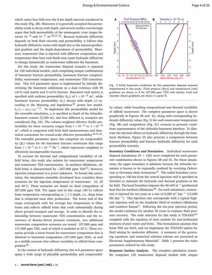
which varies four-fold over the 8 km depth interval considered inthis study (Fig. 2B). Moreover, it is generally accepted that perme-ability tends to decay with depth, and several studies convincinglyargue that bulk permeability of the seismogenic crust ranges be-tween 10−14 and 10−17 m2 24,31,32. Because hydraulic diffusivitydepends on both fluid viscosity and permeability, it follows thathydraulic diffusivity varies with depth due to the natural geother-mal gradient and the depth-dependence of permeability. More-over, wastewater that is injected with different composition andtemperature than host rock fluids may cause hydraulic diffusivityto change dynamically as wastewater infiltrates the basement.

For this study, the wastewater disposal scenario is repeatedfor 120 individual models, each comprising unique combinationsof basement fracture permeability, basement fracture compress-ibility, wastewater temperature, and wastewater TDS concentra-tion. This 4-D parameter space is implemented by initially dis-cretizing the basement subdomain as a dual continua with 98vol.% rock matrix and 2 vol.% fracture. Basement rock matrix isspecified with uniform permeability (km) of 1× 10−20 m2, whilebasement fracture permeability (k f ) decays with depth (z) ac-cording to the Manning and Ingebritsen 24 power law model:k f (z) = k0(z/z0)

−3.2. To implement this permeability model forthe ensemble simulation, z0 is specified as depth of the Arbuckle-basement contact (2,300 m), and four different k0 scenarios areconsidered (Fig. 3A). The volume-weighted effective (bulk) per-meability for these scenarios ranges from 1× 10−14 to 2× 10−18

m2, which is congruent with both field measurements and theo-retical constraints for crustal-scale effective permeability24,31,32.The ensemble parameter space also comprises six compressibil-ity (βr) values for the basement fracture continuum that rangefrom 1× 10−9 to 5× 10−12 Pa−1, which represents compliant toeffectively incompressible fractures.

To account for thermal and compositional variability of oil-field brine, this study also isolates for wastewater temperatureand wastewater TDS concentration. In northern Oklahoma, oil-field brine is characterized by ∼207,000 ppm TDS23; however,injection temperature is a priori unknown. To bound this uncer-tainty, the simulation ensemble developed here considers threescenarios for the injection temperature of wastewater: 10, 25and 40◦C. These scenarios are based on fluid composition of207,000 ppm TDS. The upper end of this range (40◦C) reflectsbrine temperature corresponding to & 1.5 depth, i.e., deep brinethat is reinjected soon after production. The lower end of thisrange corresponds with the average low temperature in Okla-homa and reflects oilfield brine that cools substantially duringabove ground transport and storage. In order to identify the re-lationship between wastewater TDS concentration and the oc-currence of density-driven pressure transients, two additionalwastewater composition scenarios are tested: 107,000 ppm and157,000 ppm TDS, each of which is modeled at 25◦C. These sce-narios provide a lower bound for wastewater composition that isidentical to basement composition (107,000 ppm TDS), as wellas a middle scenario that reflects variability in oilfield brine com-position26.

In the context of hydraulic diffusivity, this 4-D parameter spacespans a wide range of plausible permeability and compressibil-

Basement Brine

3

4

5

6

7

8

9

10

De

pth

(km

)

Fluid Pressure (MPa)

25 50 75 100 125 150 175 200 225

Temperature (°C)

3

4

5

6

7

8

9

10

De

pth

(km

)

1

Viscosity (× 10-4 Pa･s)

980 1000 1020 1040 1060 1080

Brine Density (kg m-3)

2 3 4 5 6 7 80 10 20 30 40 50 60 70 80 90100

107,000 ppm

18 °C

per km

10 M

Pa p

er km

A B

Fig. 2 Initial basement conditions for the wastewater disposal scenarioimplemented in this study. Fluid pressure (blue) and temperature (red)gradients are shown in A for 107,000 ppm TDS with density (red) andviscosity (blue) gradients are shown in panel B.

ity values, while bounding compositional and thermal variabilityof oilfield wastewater. The complete parameter space is showngraphically in Figures 3B and 3C, along with corresponding hy-draulic diffusivity values (Eq. 5) for each wastewater temperature(Fig. 3B) and composition (Fig. 3C) scenario at pressure condi-tions representative of the Arbuckle-basement interface. To illus-trate the thermal effects on hydraulic diffusivity through the base-ment thickness, Figure 3A also presents a comparison betweenfracture permeability and fracture hydraulic diffusivity for eachpermeability scenario.

Boundary Conditions and Simulation. Individual wastewaterdisposal simulations (N = 120) were completed for each param-eter combination shown in Figures 3B and 3C. For these simula-tions, the upper boundary is adiabatic because the Arbuckle for-mation is known to be regionally confined by overlying Ordovi-cian to Devonian shale formations27. The radial boundary corre-sponding to 100 km from the central injection well is specified asDirichlet to maintain the hydraulic and thermal gradients in thefar field. The basal boundary imposes the 40 mW m−2 geothermalheat flux for northern Oklahoma28. For each simulation, wastew-ater is injected for ten years at a rate of 2,080 m3 day−1 (13,000bbl day−1). This injection rate corresponds with a typical high-rate injection well on the Anadarko Shelf of northern Oklahomaand southern Kansas6. Following the ten-year injection period,the model continues for another 40 years to evaluate fluid pres-sure recovery. The code selection for this study is TOUGH329

compiled with the equation of state module for non-isothermalmixtures of pure water and brine . This formulation assumes thatbrine TDS are NaCl, and we implement the TOUGH3 option forfluid mixing by molecular diffusion. A summary of the govern-ing equations and numerical solution scheme are presented asElectronic Supplementary Materials†. Table 1 presents the staticparameters utilized for this study.

Response Surface Analysis. The complete simulation ensem-ble comprises 120 wastewater disposal models with unique



C

-2.0 -1.5 -1.0-0.5 0.0 0.5 1.0

Log Fracture Diffusivity (m2 s-1) at 21 MPa

B Wastewater 207,000 ppm TDS Wastewater Temperature 25°C

Wa

ste

wa

ter

TD

S C

on

ce

ntr

atio

n (

pp

m)

15

7,0

00

20

7,0

00

10

7,0

00

Compressibility (Pa-1) Permeability, k0 (m

2)10-11

10-10

10-9

10-14

10-13

D

A

Compressibility (Pa-1)

10-11

10-10

10-9

D

BC

A

Permeability Scenario

Permeability, k0 (m

2)

10-14

10-13

Waste

wate

r T

em

pera

ture

(°C

)25

40

10

A

5

2

3

4

6

7

8

9

10

10-1210-1310-15 10-1410-16

Fracture Permeability (m2)D

ep

th (

km

)

10-110-2 100 10110-3

Fracture Diffusivity (m2 s-1)

Arbuckle

Basement

ABCD

BCPermeability Scenario

Fig. 3 Permeability scenarios and parameter space tested for this ensemble simulation study. Panel A shows basement fracture permeability scenarios(solid lines, labeled A - D) that are based on the depth-decaying permeability model by Manning and Ingebritsen 24 . Dashed lines are fracturediffusivity corresponding to each permeability scenario for 107,000 ppm TDS basement brine, basement compressibility of 1×10−10 Pa−1, and initialconditions in Figure 2A. The complete parameter space is presented in panels B and C, where black circles denote unique combinations of basementfracture permeability, basement compressibility, and either wastewater temperature (Panel B) or wastewater TDS concentration (Panel C). Note thatall parameter combinations shown in B are for wastewater comprising 207,000 ppm TDS and all parameter combinations shown in C are for wastewatertemperature of 25◦C, thus middle slice in B is the same as top slice in C (as denoted by gray arrows). Color palette in B and C reflects hydraulicdiffusivity (Eq. 5) for each parameter combination at fluid pressure corresponding to the Arbuckle-basement contact (21 MPa).

combinations of wastewater temperature, wastewater composi-tion, depth-decaying basement permeability, and basement com-pressibility (Fig. 3B,C). Because visualizing 4-D data is cogni-tively challenging, simulation results are analyzed using three-dimensional response surface methods33. This approach con-tours a specific model feature (e.g., maximum distance to 10kPa pressure front) across two-dimensional parameter maps andthen stacks three 2-D maps on vertical axis. For this study, all re-sponse surface plots are organized as shown in Figures 3B and 3C,where permeability and compressibility are the horizontal axesand either wastewater temperature or composition is the verti-cal axis. Response surface maps of selected model features arecontoured for each wastewater scenario using all combinations offracture compressibility (βr) and permeability scenario, the latterof which is identified on Figures 4-9 by fracture permeability atthe Arbuckle-basement interface (k0).

3 Results

Long-range, diffusion-controlled pressure transients. It iswell known that individual high-rate wastewater injection wellscan drive fluid pressure transients to radial distances exceeding10-15 km (e.g.,34,35). To isolate the parametric controls on thisphenomenon, Figures 4A and 5A present response surface anal-yses for the maximum radial distance between the injection welland the 10 kPa pressure front after 10 years of wastewater injec-tion. The 10 kPa pressure front is chosen for this analysis be-cause it is generally considered the minimum stress-change toreactivate critically-stressed faults36. Across the complete sim-ulation ensemble, the 10 kPa pressure front ranges from 6 to 29

km lateral distance from the injection well after 10 years of in-jection. Response surface analyses reveal the intuitive findingthat the maximum lateral extent of the 10 kPa pressure frontincreases systematically with decreasing fracture permeability;however, this analysis also finds that long-range pressure tran-sients (i) are insensitive to wastewater temperature (Fig. 4A), (ii)increase modestly with decreasing wastewater TDS concentration(Fig. 5A), and (iii) are slightly inhibited when the fracture net-work is compliant (βr ∼ 10−9) and fracture permeability is low(k0 ∼ 10−14 m2). This is shown in Figures 4A and 5A as gradientsthat are strongly oriented in the direction of decreasing fracturepermeability with minor variations along the compressibility andwastewater temperature or composition axes. From a qualitativeperspective, this result reflects the well-known phenomenon thatfractured crystalline rocks are highly effective for transmitting flu-ids, but generally maintain little excess storage capacity.

Although this previous result is somewhat intuitive, individ-ual results for simulations bounding the parameter space showthat the shape of the 10 kPa pressure front is strongly depen-dent on the basement permeability structure (Figs. 4B-G & 5B-G). Specifically, long-range fluid pressure transients for the lowpermeability scenarios (k0 = 1×10−14 m2) reach their maximumlateral extent at shallow depths (2 – 4 km in this model) becausethe depth-decaying permeability structure impedes lateral pres-sure propagation at greater depth (Figs. 4D,E & 5D,E). In con-trast, the 10 kPa pressure fronts for the intermediate permeabilityscenarios (k0 = 1× 10−13 m2 and k0 = 5× 10−14 m2) propagateuniformly throughout the basement thickness (Fig. 4C,F & 5C,F),while the 10 kPa pressure fronts for the high-permeability sce-



Table 1 Static model parameters

k-matrix k-fracture φ ρ f βr kT cp Dm2 m2 – kg m−3 Pa−1 W m−1 ◦C−1 J kg−1 ◦C−1 m2 s−1

Arbuckle 5×10−13 – 0.1 2,500 1.7×10−10 2.2 1,000 –Basement 1×10−20 Fig 3A 0.1c,0.02d 2,080 Fig 3B 2.2 1,000 –Brine – – – variable – – – 1.1×10−9

kT -thermal conductivity. cp-specific heat. D-diffusion coefficient. c-fracture porosity. d-matrix porosity.

1000 1040 1080 1120 1160



2)10-11

10-10

10-9

10-14

10-13

2

10

0 5 10 15 20 25 30Radial Distance (km)

De

pth

(km

)

4

6

8

2

10


De

pth

(km

)

4

6

8

2

10


De

pth

(km

)

4

6

8

10

20

30

40

10

20

30

40

10

20

4030

2

10


De

pth

(km

)

4

6

8

10

20

30

40

2

10


De

pth

(km

)

4

6

8

10

20

3040

0

5

10

15

20

25

kilo

me

ters

Maximum distance

to 10 kPa ΔPf

2

10


De

pth

(km

)

4

6

8

10

20

30

40

A

BC

D

E

F G

10

25

40

Waste

wate

r T

em

pera

ture

(°C

)

Fig. 4 Response surface analysis (A) for the maximum radial distance (km) from the injection well to the 10 kPa pressure front after 10 years ofinjection for wastewater comprising 207,000 ppm TDS brine at 10, 25, and 40◦C. Panels B - G illustrate individual simulation results for models thatbound the parameter space; black contour lines denote fluid pressure change (∆Pf ) in kPa and background shading is brine density. Contour linesgreater than 40 kPa are presented with lighter stroke to facilitate visualization. Note that 10 kPa pressure front migrates substantially longer radialdistances than the wastewater plume. Detailed sections for each wastewater plume in B - G are shown in Figure 6.



2

10


De

pth

(km

)

4

6

8

E

10401000 1080 1120 1160


10-11

10-10

10-9

10-14

10-13

2

10


De

pth

(km

)

4

6

8

2

10


De

pth

(km

)

4

6

8

2

10


De

pth

(km

)

4

6

8

2

10


De

pth

(km

)

4

6

8

A

BC

F G

2

10


De

pth

(km

)

4

6

8

D


Permeability, k0 (m

2)

20

30

40 Maximum distance

to 10 kPa ΔPf

5

0

10

15

20

25

kilo

mete

rs

30

10

20

30

40

10

20

30

40

10

20

30

40

10

20

10

20

30

40

10

Waste

wate

r T

DS

Concentr

ation (

ppm

)

157,0

00

207,0

00

107,0

00

Fig. 5 Response surface analysis (A) for the maximum radial distance (km) from the injection well to the 10 kPa pressure front after 10 years ofinjection for wastewater at 25◦C and brine composition of 107,000, 157,000 and 207,000 ppm TDS. Panels B – G illustrate individual simulationresults for models that bound the parameter space; black contour lines denote fluid pressure change (∆Pf ) in kPa and background shading is brinedensity. Contour lines greater than 40 kPa are presented with lighter stroke to facilitate visualization.



narios (k0 = 5×10−13 m2) reach their maximum lateral extent atmuch greater depths (Fig. 4B,G & 5B); however, this latter trenddoes not occur for the high permeability model with 107,000 ppmTDS wastewater (Fig. 5G).

The tendency for the high permeability scenarios to cause lat-eral pressure migration at greater depths results from the rela-tionship between fracture permeability and high-TDS wastewa-ter. At 25◦C and 21 MPa fluid pressure, wastewater comprising207,000 ppm TDS has a fluid density of ∼ 1157 kg m−3, while thecorresponding density for 107,000 ppm TDS basement fluid is∼ 1081 kg m−3 25. This fluid density contrast allows the wastew-ater to sink rapidly through high permeability fractures and dis-place basement fluids, which increases fluid pressure below theinjection well and drives a short-range pressure diffusion frontlaterally. As high-density wastewater sinks deeper into the base-ment, formation fluids are drawn in from above which results in azone of underpressure near the injection well. In Oklahoma, thisprocess may explain the phenomenon in which high-rate wastew-ater injection wells operate in close proximity without pumping(i.e., gravity-fed injections)14. However, density-driven fluid flowis inhibited when wastewater and basement fluids comprise thesame TDS concentration. This explains why the 10 kPa pressurefront advances uniformly through the basement for the high per-meability model with 107,000 ppm TDS wastewater (Fig. 5G).

Local-scale, density-driven pressure transients. The relation-ship between fluid composition and earthquake occurrence wasfirst identified by Pollyea et al. 23 , which used numerical simula-tion to show that density-driven pressure transients sink at thesame rate as mean annual earthquake depths increase within sev-eral Oklahoma counties. The study also found that the relativeproportion of high-magnitude earthquakes increases at 8+ kmdepth. While the earthquake rate at 8+ km depth is small incomparison to more shallow depths, density-driven pressure tran-sients may persist in the seismogenic zone over much longer timescales than pressure fronts governed by pressure diffusion alone.As a result, density-driven pressure transients may prolong earth-quake hazard in regions where wastewater is characterized bysubstantially higher TDS concentration than fluids in the seismo-genic basement.

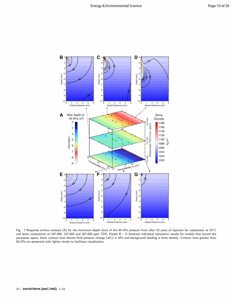
To explore parametric controls on density-driven pressure tran-sients, Figures 6A and 7A present response surface analyses forthe maximum depth of 40 kPa pressure change after 10 yearsof injection at 2,080 m3 day−1 (13,000 bbl day−1). The 40 kPapressure front is considered for this analysis because its depth isstrongly influenced by sinking, high-density wastewater duringthe 10-year injection period (Fig. 6C-G, 7B-D). As with laterallong-range (diffusion-controlled) pressure transients, this analy-sis reveals that basement permeability structure is the first-ordercontrol on the depth to which density-driven pressure transientsmay sink. For wastewater composition of 207,000 ppm TDS,the 40 kPa pressure front reaches ∼5 km, ∼6 km, and ∼7 kmdepth after 10 years for the low, intermediate, and high perme-ability scenarios, respectively (Fig. 6B-G). These results show thatdensity-driven pressure transients also emerge when wastewatercomprises 157,000 ppm TDS (Fig. 7B-D); however, the depth

to the 40 kPa pressure front is ∼1 - 1.5 km less than the cor-responding high-TDS injection scenarios. Because the 40 kPapressure front is driven largely by sinking, high-TDS wastewa-ter, the density differential between wastewater and basementfluids is a fundamental control on density-driven pressure tran-sients. For the high-TDS wastewater scenarios (207,000 ppm),the density differential between 25◦C wastewater and basementfluids is ∼76 kg m−3 at the Arbuckle-basement interface, butthis difference reduces to ∼ 37 kg m−3 for wastewater compris-ing 157,000 ppm TDS. This result implies that even modest den-sity differences may cause density-driven pressure transients todevelop locally below injection wells when permeability is highenough to permit density-driven fluid flow into the basement. Incontrast, the simulation ensemble also reveals that density-drivenpressure transients do not occur when (i) permeability is insuf-ficient (. 10−14 m2) to allow density-driven fluid flow into thebasement (Fig. 6B,E & 7B,E) and (ii) the density contrast betweenwastewater and basement fluids is insufficient to cause density-driven fluid flow (Fig. 7E-G). As a consequence, fluid pressuretransients are driven primarily by pressure diffusion when base-ment fracture permeability is low (e.g., . 5× 10−14 m2) and/orwastewater and basement fluids comprise similar fluid density.

Closer inspection of Figure 6B-G reveals that wastewater in-jection temperature imposes a second-order control on the depthand magnitude of density-driven pressure transients because the40 kPa pressure front becomes systematically deeper as wastew-ater injection temperature decreases (Fig. 6A). This phenomenonoccurs because the wastewater density is ∼1148 kg m−3 at 40◦Cand 21 MPa, but increases to ∼1164 kg m−3 at 10◦C and 21MPa. The additional load imposed by lower temperature wastew-ater increases the fluid potential causing the wastewater plumeto sink deeper into the seismogenic zone. These thermal effectsfurther reinforce the development of density-driven pressure tran-sients because fluid density in the basement decreases with depthdue to the geothermal gradient (Fig. 2B). As a result, the fluiddensity contrast is maintained as wastewater sinks deeper intothe seismogenic basement. To illustrate this phenomenon, in-dividual simulation results for high permeability scenarios with207,000 ppm TDS wastewater show that the maximum fluid pres-sure change (∆Pf ) is 110 kPa between 6.75 and 7.25 km depthfor wastewater injection temperature of 10◦C (Fig. 6G); whereas,the maximum ∆Pf is 100 kPa between 6.5 and 7 km depth whenwastewater is 40◦C (Fig. 6D). This general pattern is also appar-ent for the corresponding intermediate permeability scenarios,but low permeability scenarios prevent density-driven pressuretransients from entering the basement within the first 10 years ofinjection (Fig. 6B,E).

In aggregate, this study finds that density-driven pressure tran-sients may cause effective stress change in the seismogenic base-ment when (i) basement fracture permeability exceeds ∼ 5×10−14 m2 at the basement contact and (ii) the fluid density con-trast between wastewater and basement fluids exceeds ∼37 kgm−3. Results for the high- and intermediate-permeability scenar-ios tested here can be further generalized as (i) basement frac-ture permeability and fluid density contrast are first-order con-trols on the depth interval and magnitude density-driven pressure



4.0

4.5

5.0

5.5

6.0

6.5

7.0

7.5

8.0

8.5

9.0

Max depth to

40 kPa ΔPf

kilo

mete

rs


10-11

10-10

10-9

Permeability, k0 (m

2)

10-14

10-13

2

2

3

4

5

6

7

8

9

100 1 3 4 5

Radial Distance (km)

De

pth

(km

)

40

30

20

50

2

2

3

4

5

6

7

8

9

100 1 3 4 5


De

pth

(km

)

2

2

3

4

5

6

7

8

9

100 1 3 4 5


De

pth

(km

)

2

2

3

4

5

6

7

8

9

100 1 3 4 5


De

pth

(km

)

2

2

3

4

5

6

7

8

9

100 1 3 4 5


De

pth

(km

)

30

40

50

20

10

1000

1020

1040

1060

1080

1100

1120

1140

1160

1180

kg m

-3

Brine

Density

30

40

50

20

2

2

3

4

5

6

7

8

9

100 1 3 4 5


De

pth

(km

) 40

50

30

20

30

40

50

10

20

30

30

40

50

A

B C D

E F G

10

25

40

Wa

ste

wa

ter

Te

mp

era

ture

(°C

)

Fig. 6 Response surface analysis (A) for the maximum depth (km) of the 40 kPa pressure front after 10 years of injection with wastewater comprising207,000 ppm TDS brine at 10, 25, and 40◦C. Panels B – G illustrate individual simulation results for models that bound the parameter space; blackcontour lines denote fluid pressure change (∆Pf ) in kPa and background shading is brine density. Contour lines greater than 50 kPa are presented withlighter stroke to facilitate visualization.



2

2

3

4

5

6

7

8

9

100 1 3 4 5


De

pth

(km

)

2

3

Max depth to

40 kPa ΔPf

kilo

mete

rs


10-11

10-10

10-9

Permeability, k0 (m

2)

10-14

10-13

2

2

3

4

5

6

7

8

9

100 1 3 4 5


De

pth

(km

)

2

2

3

4

5

6

7

8

9

100 1 3 4 5


De

pth

(km

)

2

2

3

4

5

6

7

8

9

100 1 3 4 5


De

pth

(km

)

2

2

3

4

5

6

7

8

9

100 1 3 4 5


De

pth

(km

)

1000

1020

1040

1060

1080

1100

1120

1140

1160

1180

kg m

-3

Brine

Density

2

2

3

4

5

6

7

8

9

100 1 3 4 5


De

pth

(km

)

30

40

50

A

B C D

E F G

20

30

40

50

107,0

00

157,0

00

207,0

00

Wa

ste

wa

ter

TD

S C

on

c.

(pp

m)

4

5

6

7

8

9

scale 40%

10

40 30 20

30

40

20

40

30

20

50

Fig. 7 Response surface analysis (A) for the maximum depth (km) of the 40 kPa pressure front after 10 years of injection for wastewater at 25◦Cand brine composition of 107,000, 157,000 and 207,000 ppm TDS. Panels B – G illustrate individual simulation results for models that bound theparameter space; black contour lines denote fluid pressure change (∆Pf ) in kPa and background shading is brine density. Contour lines greater than50 kPa are presented with lighter stroke to facilitate visualization.



A

10

25

40

Waste

wate

r T

em

pera

ture

(°C

)


2)10-11

10-10

10-9

10-14

10-13

0Maximum ΔPf Below Well at 5 km Depth (kPa)


2)10-11

10-10

10-9

10-14

10-13

15030 60 90 120 0 5 10 15 20 25 30Time to Maximum ΔPf at 5 km Depth (years)

B

Injection Post-Injection Recovery

C


2)10-11

10-10

10-9

10-14

10-13


2)10-11

10-10

10-9

10-14

10-13

D

Waste

wate

r T

DS

Conc. (1

03 p

pm

)157

207

107

Waste

wate

r T

DS

Concentr

ation (

ppm

)

157,0

00

207,0

00

107,0

00

Waste

wate

r T

em

pera

ture

(°C

)

25

40

10

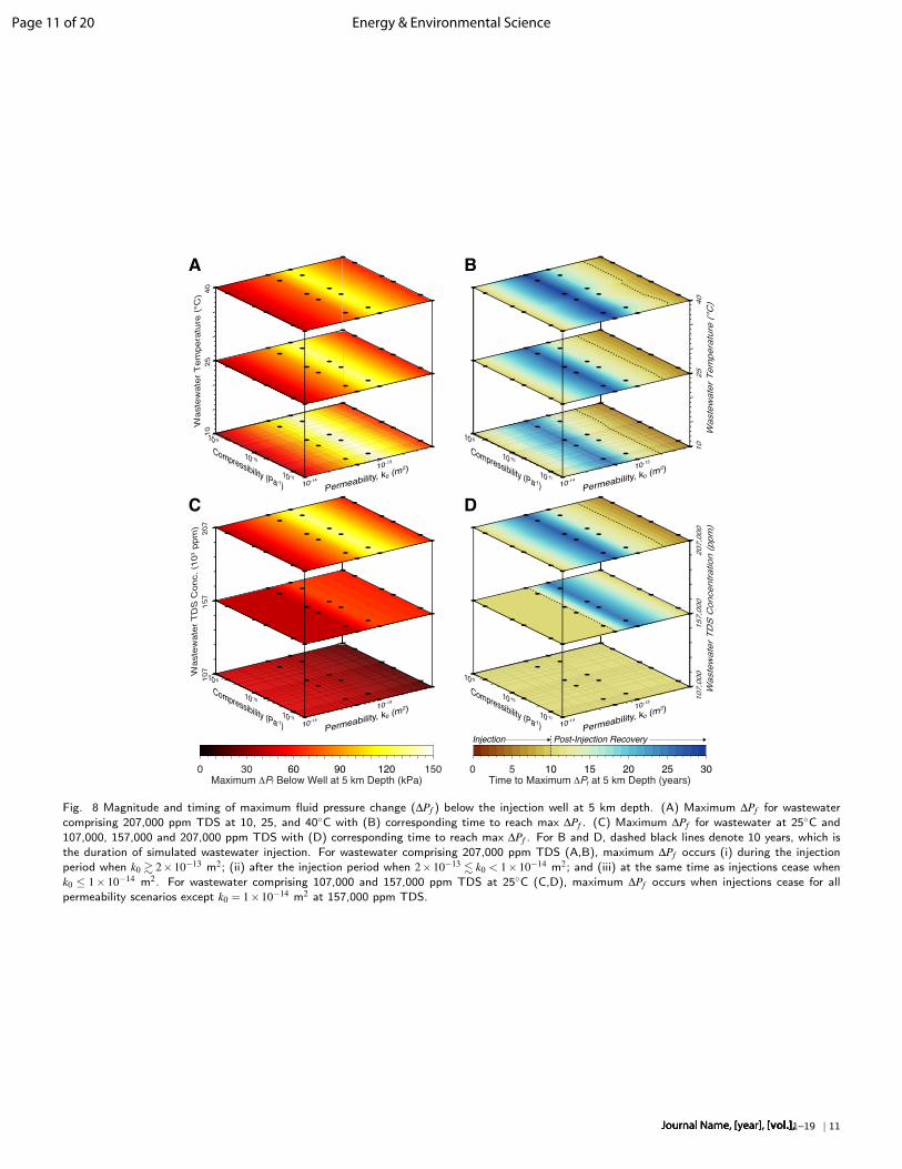
Fig. 8 Magnitude and timing of maximum fluid pressure change (∆Pf ) below the injection well at 5 km depth. (A) Maximum ∆Pf for wastewatercomprising 207,000 ppm TDS at 10, 25, and 40◦C with (B) corresponding time to reach max ∆Pf . (C) Maximum ∆Pf for wastewater at 25◦C and107,000, 157,000 and 207,000 ppm TDS with (D) corresponding time to reach max ∆Pf . For B and D, dashed black lines denote 10 years, which isthe duration of simulated wastewater injection. For wastewater comprising 207,000 ppm TDS (A,B), maximum ∆Pf occurs (i) during the injectionperiod when k0 & 2×10−13 m2; (ii) after the injection period when 2×10−13 . k0 < 1×10−14 m2; and (iii) at the same time as injections cease whenk0 ≤ 1× 10−14 m2. For wastewater comprising 107,000 and 157,000 ppm TDS at 25◦C (C,D), maximum ∆Pf occurs when injections cease for allpermeability scenarios except k0 = 1×10−14 m2 at 157,000 ppm TDS.



transients, (ii) wastewater injection temperature imposes second-order effects with cooler (higher density) wastewater drivingpressure transients deeper and to higher magnitude, and (iii)density-driven pressure transients are insensitive to basementcompressibility.

Post-injection pressure recovery. The rate of injection-inducedearthquakes in Oklahoma has fallen each year since 20156;however, wastewater disposal operations have been widespreadthroughout the region since 20093,6. Because oilfield brine innorthern and eastern Oklahoma is characterized by TDS concen-tration between 175,000 and 235,000 ppm26, the persistenceof density-driven pressure transients may delay the time scaleover which seismicity reaches background levels23. To under-stand the temporal dimension of density-driven pressure tran-sients, Figure 8 presents response surface analyses for maximum∆Pf recorded directly below the injection well at 5 km depth,along with corresponding response patterns for the time at whichmaximum ∆Pf occurs. At 5 km depth, maximum ∆Pf ranges from20 to 150 kPa (Fig. 8A,C); however, the response patterns reveal anumber of counterintuitive findings. For example, the maximum∆Pf at 5 km depth occurs for model scenarios in which wastew-ater composition is 207,000 ppm TDS, injection temperature is10◦C and k0 is 1× 10−13 m2. This result is congruent with highTDS and low temperature (thus higher density) wastewater lo-cally increasing pressure magnitude below injection wells, but itis not readily apparent why maximum ∆Pf at 5 km depth occursat one of the intermediate permeability scenarios.

The phenomenon in which ∆Pf at 5 km depth is greatest forintermediate permeability scenarios can be explained by decou-pling the two different pressure propagation mechanisms oper-ating within the wastewater disposal system: (i) wellhead pres-sure diffusion and (ii) advective transport of high-density brine.To do so, time-series ∆Pf data were recorded below the injec-tion at a depth of 5 km (Fig. S1† & S2†) and response surfacemaps for time corresponding to maximum ∆Pf at 5 km depth areshown in Figure 8B,D. These results show that the maximum ∆Pf

at 5 km depth tends to occur (i) before injection operations ceasefor the high TDS (207,000 ppm) scenarios with high permeabil-ity (k0 = 5× 10−13 m2), (ii) after injection operations cease forthe intermediate permeability scenarios (k0 = 1× 10−13m2 andk0 = 5× 10−14 m2), and (iii) contemporaneously with the end ofthe 10-year injection period for the both the low permeability sce-narios (k0 = 1×10−14 m2) and the low TDS wastewater (107,000ppm) scenarios. For model scenarios with high TDS wastewa-ter and high fracture permeability, formation fluids are readilydisplaced as wastewater sinks (Figs. 6D,G), so advective trans-port of high-density wastewater is the primary mechanism driv-ing fluid pressure accumulation. As a result, ∆Pf at 5 km depthbegins rapidly increasing upon arrival of the sinking wastewaterplume. When the wastewater plume passes through 5 km depth,lower density formation fluids flow back into the path of the brineplume, which, for this model scenario, occurs before injectionstop (Fig. S1†). This is in stark contrast to the lowest permeabilityscenarios (k0 = 1×10−14 m2), which inhibit advective wastewatertransport into the basement (Figs. 6B,E & 7B,E), so wellhead pres-

sure diffusion is the primary process driving pressure transientsinto the seismogenic zone. Pressure diffusion also governs ∆Pf

for model scenarios comprising wastewater with 107,000 ppmTDS because wastewater and basement fluids comprise the sameTDS concentration, and thus density, at injection depth so second-order thermal effects are the only process that can cause density-driven pressure transients. For these high-permeability and low-TDS wastewater scenarios, Figure S1† and S2† show that ∆Pf in-creases monotonically at 5 km depth until pumping stops, whichis congruent with a Theis curve. Because ∆Pf at 5 km depth is gov-erned by advective brine transport for the high permeability sce-narios and pressure diffusion for the low permeability scenarios,then pressure accumulation at 5 km depth for the intermediatepermeability scenarios is the superposition of wellhead pressureand density-driven pressure transients. This superposition occursbecause wastewater can enter the upper basement within the 10-year injection period (Fig. 6C,F & 7C), but formation fluid cannotbe displaced as quickly as for the high permeability scenarios sowellhead pressure builds up and adds to the ∆Pf signal. Wheninjections stop, wellhead pressure no longer contributes to the∆Pf signal and there is a brief decline in pressure build-up; how-ever, fluid pressure begins rising again as high-TDS wastewateraccumulates between 4 and 5 km depth (Fig. S1† & S2†) wherefracture permeability falls below 5×10−14 m2.

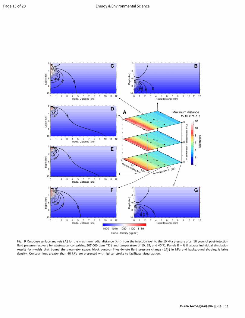
The temporal dimensions of ∆Pf variations imply that base-ment permeability, wastewater composition and wastewater tem-perature each play fundamental roles in fluid pressure recov-ery after injection operations cease. To evaluate how far-field,diffusion-controlled pressure fronts respond during post-injectionfluid pressure recovery, Figures 9A and 10A present response sur-face maps for maximum distance to the 10 kPa pressure frontafter ten years of post-injection fluid pressure recovery. This anal-ysis indicates that far-field pressure recovery is also governed pri-marily by basement permeability; however, inspection of selectedsimulation results shows that residual fluid pressure remains lo-cally elevated within a 1 – 2 km radius of injection wells even after10 years of recovery, regardless of basement permeability struc-ture (Figs. 9B-G & 10B-D). Residual fluid pressure is maintainedbecause loading conditions imposed by high-density wastewaterpersist until fluid composition equilibrates with the surroundinghost-rock fluids. This equilibration period is governed by fluidmixing, which is the result of both advective transport and molec-ular (Fickian) diffusion. In this context, advective transport slowssignificantly as basement permeability decreases and Fickian dif-fusion occurs over much longer timescales.

The persistence of residual fluid pressure in the seismogenicbasement begs the question of whether or not fluid pressure con-tinues increasing within the basement during post-injection re-covery. The individual results shown in Figures 9B-G and 10B-G indicate that far-field (diffusion-controlled) pressure transientscollapse in the absence of wellhead pressure. This implies thatrock volume in the far field reaches maximum ∆Pf when (or soonafter) injection operations cease. This result is further supportedby time-series ∆Pf data recorded for each simulation at 4 km ra-dial distance from the injection well and 4.5 km depth (Figs. S3†

& S4†). The data show that ∆Pf in the far-field exhibit diffusion-



2

10


De

pth

(km

)

4

6

8

2 3 5 7 119

2

10


De

pth

(km

)

4

6

8

2 3 5 7 119

2

10


De

pth

(km

)

4

6

8

2 3 5 7 119

2

10


De

pth

(km

)

4

6

8

2 3 5 7 119


2

10


De

pth

(km

)

4

6

8

2 3 5 7 119

1000 1040 1080 1120 1160



2)10-11

10-10

10-9

10-14

10-13

10

0

2

4

6

8

10

kilo

mete

rs

Maximum distance

to 10 kPa ΔPf

A

B

12

C

GF

E20

30

40

0

10

20304

0

0

2

10


De

pth

(km

)

4

6

8

2 3 5 7 119

D

10

2030

10

20

30

1020

4030

0

0

10

20

30

40

10

25

40

Waste

wate

r T

em

pera

ture

(°C

)

Fig. 9 Response surface analysis (A) for the maximum radial distance (km) from the injection well to the 10 kPa pressure after 10 years of post-injectionfluid pressure recovery for wastewater comprising 207,000 ppm TDS and temperature of 10, 25, and 40◦C. Panels B – G illustrate individual simulationresults for models that bound the parameter space; black contour lines denote fluid pressure change (∆Pf ) in kPa and background shading is brinedensity. Contour lines greater than 40 kPa are presented with lighter stroke to facilitate visualization.



2

100


Depth

(km

)

4

6

8

1 2 3 4 5

10

A

Brine

Density

Maximum distance

to 10 kPa ΔPf


10-11

10-10

10-9

10-14

10-13

Permeability, k0 (m

2)

107

157

207

Waste

wate

r T

DS

Con

c. (1

03 p

pm

)

5

0

10

15

20

kilo

mete

rs

2

10

Depth

(km

)

4

6

8

0 2 4 6 8 10 12 14 16 18 20


10

2

100


Depth

(km

)

4

6

8

1 2 3 4 5

10

2

100


Depth

(km

)

4

6

8

1 2 3 4 5

10

0

2

10

Depth

(km

)

4

6

8

0 2 4 6 8 10 12 14 16 18 20


D2

100


Depth

(km

)

4

6

8

1 2 3 4 5

B

1040

1000

1080

1120

1160

kg m

-3

C

E F G

10

30 20

0

10

3020

0

20

Fig. 10 Response surface analysis (A) for the maximum radial distance (km) from the injection well to the 10 kPa pressure after 10 years of post-injection fluid pressure recovery for wastewater at 25◦C and brine composition of 107,000, 157,000 and 207,000 ppm TDS. Panels B – G illustrateindividual simulation results for models that bound the parameter space; black contour lines denote fluid pressure change (∆Pf ) in kPa and backgroundshading is brine density. Contour lines greater than 40 kPa are presented with lighter stroke to facilitate visualization.



controlled (Theis-like) patterns for all simulations with peak ∆Pf

when injections cease. These results imply that both effectivestress change and solid elastic stress transfer reach their maxi-mum lateral extent during (or soon after) active injection opera-tions.

Although far-field pressure transients peak during the injectionperiod for all permeability scenarios, fluid pressure continues in-creasing locally below the injection well for up to 20 years afterinjections cease in both intermediate and high permeability sce-narios (Figs. S3† & S4†). For example, ∆Pf after 10 years of injec-tion reaches 40 kPa at 8 km depth for the high-permeability sce-nario illustrated in Figure 4B; however, this increases 80 kPa aftera decade of recovery (Fig. 9B). This phenomenon reflects a feed-back between high-TDS wastewater and the geothermal gradientbecause the sinking wastewater plume passes through systemati-cally warmer and lower density host rock fluids, so the fluid den-sity contrast driving advective pressure transients is maintainedeven as wastewater mixes with host rock fluids. Local regions ofincreasing post-injection fluid pressure also occur for the inter-mediate permeability scenarios, albeit at shallower depths; how-ever, this phenomenon does not occur for the lowest permeabil-ity scenarios because wastewater cannot sink beyond the upper-most basement. In natural geologic systems, these results suggestthat high-TDS wastewater may continue flowing through inter-connected fault and fracture networks for years after injectionoperations cease. Generalizing the parametric controls on fluidpressure recovery for oilfield wastewater disposal suggests that(i) far-field pressure recovery is rapid and governed by fracturepermeability, (ii) when wastewater sinks into the basement, fluidpressure continues increasing locally below injection wells evenafter injection operations cease, and (iii) the geothermal gradi-ent maintains density-driven pressure transients because base-ment fluids become systematically warmer (and lower density)with increasing depth.

4 DiscussionThere is now general consensus that wastewater disposal oper-ations cause fluid pressure transients that induce earthquakesby (i) decreasing effective normal stresses on optimally-orientedfaults and (ii) driving solid elastic stress transfer ahead of thepressure front. This study adds an important new spatiotempo-ral perspective to this conceptual model by integrating the ef-fects of wastewater and basement fluid composition, the crustalscale geothermal gradient, and PTX-dependent fluid properties.Specifically, wastewater disposal operations cause long-range,diffusion-controlled pressure fronts that propagate radially in ac-cordance with root-time scaling, while also driving solid elasticstress transfer ahead of the pressure front10. When wastewa-ter comprises higher TDS concentration than basement fluids, thehigh-density wastewater sinks , which locally increases fluid pres-sure below the injection well23 (Fig. 11A). After injection opera-tions cease, the long-range pressure front collapses rapidly, whilethe density-driven pressure front continues sinking deeper intothe seismogenic basement (Fig. 11B). In this context, maximumfluid pressure in the far-field occurs when (or soon after) injectionoperations cease, while density-driven fluid flow may continue in-

A

B

not to scale

Diffusion-controlled

long-range pressure frontDensity-driven local-scale

pressure front

Diffusion-controlled

pressure front collapses

Density-driven front continues sinking

& increasing pressure

Solid elastic stress transfer > effective stress change

Fig. 11 Schematic illustration of mechanisms driving fluid pressure tran-sients during oilfield wastewater disposal when (i) the disposal reservoiris hydraulically connected to crystalline basement and (ii) wastewaterdensity is & 37 kg m−3 greater than basement fluids due to thermal andcompositional differences between the fluids. During injection operations(A), diffusion-controlled pressure transients (black arrows) propagate ra-dially from well in accordance with root-time spatial scaling, which drivessolid elastic stressing ahead of the pressure front (white arrows). As thisoccurs, wastewater sinks into the upper basement and density-drivenpressure transients (blue shading) develop. After injection operations(B), the long-range pressure front collapses, while density-driven pressuretransients continue sinking deeper into the basement. This latter processis reinforced by the natural geothermal gradient (white-to-red shading)because the density contrast between wastewater and basement fluids ismaintained even as the wastewater mixes with basement fluids.

creasing fluid pressure locally below injection wells for 10+ years.Conceptually, the timing and magnitude of density-driven pres-

sure transients are governed by basement permeability structureand PTX conditions of wastewater and basement fluids. From amechanistic perspective, the persistence of density-driven pres-sure transients is attributable to the density contrast betweenhigh-TDS wastewater and basement fluids, and this contrastincreases with depth due to the natural geothermal gradient.Specifically, sinking high-TDS wastewater passes through progres-sively higher temperature (and thus lower density) basement flu-ids, which maintains the density contrast even as wastewater andbasement fluids mix. Interestingly, the relationship between solidelastic stress transfer and local-scale density-driven pressure tran-sients remains an open question, but from a qualitative perspec-tive, it seems plausible that (i) the excess load imposed by high-TDS wastewater would increase the magnitude of solid elasticstressing locally below injection wells and (ii) density-driven pres-sure fronts would drive elastic stressing to systematically greaterdepths as the pressure front sinks. This implies that elastic stress-ing may persist locally over time scales that are comparable todensity-driven pressure transients (Fig. 11B); however, further re-search is needed in this area.



Washington

Oregon

California

Idaho

Nevada

ArizonaNew Mexico

Utah

Colorado

MontanaNorth

Dakota

South Dakota

Nebraska

Louisiana

Missouri

Minnesota

Wisconsin

Mississippi

Florida

Georgia

South

Carolina

North Carolina

Virginia

Maryland

Delaware

New Jersey

Connecticut

Mass.

New Hampshire

VermontMaine

Rhode Island

Montana

ColoradoColorado

MontanaMontana

MONTANA

THRUST BELT

BIG HORN

POWER RIVER

WILLISTON

GREEN RIVER

DENVER

BASINUNITA-PICEANCE

PARADOXSAN JOAQUIN

BASIN

LOS ANGELES BASIN

VENTURA BASIN SAN JUAN

RATON

BASIN

MARFA

PERMIAN

PALO DURO

FORT

WORTH

WESTERN GULF

TX-LA-MS SALT

BLACK WARRIOR

VALLEY & RIDGEARKOMA

ANADARKO

CHEROKEE

PLATFORM

FOREST

CITY ILLINOIS

BASIN

APPALACHIAN

BASIN

MICHIGAN

BASIN

0 250 500 1,000

kilometers

Fig. 12 Map of oil and gas basins across the coterminous United States37 (blue shading), unconventional tight oil and shale plays38 (yellow shading),and location of conventional hydrocarbon wells with TDS samples reported to be ≥200,000 ppm (red circles)26.

In order for density-driven pressure transients to occur,wastewater must comprise higher TDS concentration than base-ment fluids. In this context, oilfield wastewater originates asbasin brine that co-exists with oil and gas deposits in sedimen-tary basins. These fluids are generally considered to be remnantseawater that has been trapped within sedimentary formationssince the time of deposition39; however, brine migration and en-richment remain active areas of research due to their relation-ship with oil and gas deposits and ore formation40. In a recentreview of injection-induced seismicity, Foulger et al. 41 identifiesseveral regions where wastewater disposal operations are likelyto have caused earthquakes. For example, earthquake sequencesin the Sichuan Basin, China have been attributed to wastewaterdisposal42. In this region, the TDS concentration of basin brinegenerally exceeds 150,000 ppm with several samples exceeding300,000 ppm TDS43. Within the coterminous United States,where injection-induced earthquakes are now common, the USGSNational Produced Waters Geochemical Database (NPWGD)26

indicates that the TDS concentration of oilfield brine exceeds200,000 ppm throughout many of the oil- and gas-producingbasins nationwide (Fig. 12). In contrast, the NPWGD indicatesthat Precambrian basement fluids are characterized by lowermean TDS concentrations of ∼107,000 ppm and ∼39,000 ppmwithin the Anadarko Shelf (southern Kansas) and Permian Basin(southeastern New Mexico), respectively26. Although NPWGDcontains only 15 records for Precambrian basement fluids (outof ∼114,000 records), these data are congruent with Bucher andStober 44 who found that basement TDS concentration is less than100,000 ppm at 22 out of 24 international sites. These data im-ply that basement TDS concentration is generally below 100,000

ppm.

The numerical simulations developed for this study sug-gest that wastewater disposal operations may be susceptible todensity-driven pressure transients if the following criteria aremet: (i) basement fluids are .100,000 ppm TDS and oilfield brine(wastewater) is &150,000 ppm TDS, although susceptibility in-creases dramatically for TDS concentration &200,000 ppm TDS;(ii) wastewater disposal wells are in hydraulic connection withthe underlying basement; and (iii) basement fracture permeabil-ity is & 5×10−14 m2. Although basement fracture permeability isgenerally unknown, oilfield brine is characterized by TDS concen-tration in excess of 150,000 ppm throughout numerous oil andgas basins worldwide, e.g., Sichuan Basin, China43, Baltic Basin,Poland45, Northwest Carboniferous Basin, UK46, Paris Basin,France47, to name a few. In the central United States, numer-ous unconventional oil and gas plays occur in sedimentary basinswith brine composition reported to be in excess of 200,000 ppmTDS, e.g., Permian and Anadarko Basins26 (Fig. 12). Becausebasement fluids are generally below 100,000 ppm TDS26,44, oil-field wastewater disposal in basins with &200,000 ppm TDS brine(Fig. 12) may be susceptible to the long-term effects of density-driven pressure transients if disposal wells are in hydraulic com-munication with the underlying basement. This susceptibility isparticularly relevant for unconventional plays (tight oil and shalegas) because they are characterized by low permeability, so pro-duced brine cannot be reinjected back into the producing forma-tion (i.e., waterflooding). As a result, brine produced from uncon-ventional hydrocarbon recovery is reinjected into non-producinggeologic formations, which may result in fluid pressure transientsthat trigger earthquakes.



The most prominent case study for injection-induced seismicityis the State of Oklahoma, USA, where the annual M3+ earth-quake rate increased from approximately one per year before2009 to more then two M3+ earthquakes per day in 20156. Itis now well-known that oilfield wastewater disposal from uncon-ventional plays contributed to this dramatic rise in earthquakefrequency3,4,6. In this region, oilfield brine from the MississippiLime and Hunton formations is characterized by ∼175,000 to235,000 ppm TDS23,26. These fluids are then reinjected intothe basal Arbuckle formation, which is in hydraulic communi-cation with the seismogenic basement5. And while earthquakefrequency peaked in 20156, recent research shows that density-driven pressure transients from high-TDS wastewater continuedriving earthquakes systematically deeper23. Based on these cri-teria, the Permian Basin (Fig. 12) may also be susceptible to theeffects of density-driven pressure transients because (i) uncon-ventional oil and gas production, wastewater disposal, and earth-quake occurrence have been increasing steadily since 201548; (ii)the water cut (ratio of produced brine to total fluid withdrawals)is ∼70%49; and (iii) wastewater disposal occurs in the Ellen-burger Group50, which is a deep carbonate platform sequencethat is juxtaposed with the underlying basement. In contrast, theWilliston and Appalachian Basins (Fig. 12) may be less suscepti-ble to density-driven pressure transients because there are fewerwastewater disposal wells in operation and the water cut is lowin comparison to the Permian Basin and Anadarko Shelf49,51.

5 ConclusionsThere is now ample evidence to suggest that oilfield wastewa-ter disposal induces fluid pressure transients that cause earth-quakes by (i) decreasing effective normal stress on optimally-oriented faults (e.g.,5,35) and (ii) driving solid elastic stress trans-fer ahead of the pressure front (e.g.,7,10). This implies thatfluid pressure transients are the first-order process responsiblefor injection-induced earthquakes. Numerous modeling studiesshow that pressure diffusion drives long-range fluid pressure tran-sients during oilfield wastewater disposal5,7,11,13,15,17,19,22; how-ever, Pollyea et al. 23 recently found that density-driven fluid flowalso drives pressure transients into the seismogenic zone whenthere is a strong density contrast between wastewater and base-ment fluids. The present study implements ensemble simulationmethods to isolate the hydraulic, thermal, geochemical, and ge-ologic controls on both diffusion-controlled and density-drivenfluid pressure transients. For wastewater disposal wells that are inhydraulic communication with underlying basement, results fromthis study can be generalized as:

1. Long-range, diffusion-controlled pressure transients are gov-erned by basement fracture permeability, but they are gen-erally insensitive to wastewater chemistry, injection temper-ature and basement fracture compressibility;

2. Density-driven pressure transients are dependent on thedensity differential between wastewater and basement fluidsand require sufficient basement fracture permeability to al-low density-driven fluid flow. Results from this study suggestthat density-driven pressure transients may develop when

the following criteria are met: (i) basement fracture perme-ability is & 5×10−14 m2 at seismogenic depth, (ii) basementfluid composition is .100,000 ppm TDS, and (iii) wastewa-ter comprises &150,000 ppm TDS ; however, the depth andmagnitude of density-driven pressure transients increasesdramatically when wastewater TDS concentration exceeds200,000 ppm;

3. When wastewater injections cease, the absence of well-head pressure causes far-field (diffusion-controlled) pres-sure fronts to collapse rapidly; however, density-driven pres-sure transients continue to locally increase fluid pressure atsystematically greater depths for 10+ years;

4. The long-term persistence of density-driven pressure tran-sients is reinforced by the crustal-scale geothermal gradientbecause high-TDS wastewater sinks through systematicallywarmer (and lower density) basement fluids, thus maintain-ing the fluid density contrast;

5. Wastewater temperature is a second-order control on thedepth and magnitude of density-driven pressure transientsbecause (i) cooler wastewater comprises higher density,which increases the dynamic load and (ii) basement fluiddensity decreases with depth as temperature increases.

These conclusions present a new perspective on the hydraulicsof induced seismicity by accounting for wastewater chemistry,PTX-dependent fluid properties and depth-varying geologic prop-erties. This new perspective enhances the generally accepted con-ceptual model of injection-induced seismicity by incorporatingthe effects of density-driven pressure transients, which continuemigrating through seismogenic zone long after injection opera-tions cease23. This new conceptual model (Fig. 11) is applicableto oil and gas basins where oilfield wastewater is characterizedby &150,000 ppm TDS, which are widespread globally.

In closing this study, it is important to state clearly that themodel scenario developed herein is based on numerous geo-logic and operational characteristics of the Anadarko Shelf; how-ever, the model itself is hypothetical and does not reproducea real world site. In addition, the geology reproduced in thisstudy is highly idealized because site-scale fracture networks inthe crystalline basement are poorly characterized in compari-son with resource-bearing sedimentary formations. As a result,this study yields insights about the physics governing injection-induced pressure transients, and thus effective stress change. Innatural geologic systems, the spatial patterns of density-drivenpressure transients will be strongly dependent on heterogeneousand anisotropic hydraulic properties of basement fracture net-works and they are likely to vary in comparison to the idealizedschematic presented in Figure 11. As a result, the application ofthis study for site-scale earthquake hazard analysis requires sub-stantial investments for characterizing the hydraulic attributes ofthe seismogenic basement. Because injection-induced pressuretransients are a fundamental component of numerous geoenergytechnologies, e.g., enhanced geothermal systems52 and geologiccarbon sequestration53, the authors hope that insights gained



from this study further motivate frontier research into the hy-draulic characteristics of faults and fractures in the seismogenicbasement.

Conflicts of interestThere are no conflicts to declare.

AcknowledgementsThe authors thank Dr. Martin C. Chapman for insightful dis-cussions about injection-induced earthquakes. The authors aregrateful to two anonymous reviewers who provided thought-ful comments that dramatically improved the quality of thismanuscript. Computational resources were provided by Ad-vanced Research Computing at Virginia Tech. This study is basedupon work supported by the U.S. Geological Survey under GrantNo. G19AP00011. The views and conclusions contained in thisdocument are those of the authors and should not be interpretedas representing the opinions or policies of the U.S. Geological Sur-vey. Mention of trade names or commercial products does notconstitute their endorsement by the U.S. Geological Survey.

Notes and references1 W. L. Ellsworth, Science, 2013, 341, 1225942.2 S. E. Hough, Bulletin of the Seismological Society of America,

2014, 104, 2619–2626.3 M. Weingarten, S. Ge, J. W. Godt, B. A. Bekins and J. L. Ru-

binstein, Science, 2015, 348, 1336–1340.4 K. M. Keranen, H. M. Savage, G. A. Abers and E. S. Cochran,

Geology, 2013, 41, 699–702.5 K. M. Keranen, M. Weingarten, G. A. Abers, B. A. Bekins and

S. Ge, Science, 2014, 345, 448–451.6 R. M. Pollyea, N. Mohammadi, J. E. Taylor and M. C. Chap-

man, Geology, 2018, 46, 215–218.7 T. Goebel, M. Weingarten, X. Chen, J. Haffener and E. Brod-

sky, Earth and Planetary Science Letters, 2017, 472, 50–61.8 NRC, Induced Seismicity Potential in Energy Technologies, Na-

tional Academies Press, 2013.9 P. Bhattacharya and R. C. Viesca, Science, 2019, 364, 464–

468.10 T. H. Goebel and E. E. Brodsky, Science, 2018, 361, 899–904.11 G. Zhai, M. Shirzaei, M. Manga and X. Chen, Proceedings of

the National Academy of Sciences, 2019, 116, 16228–16233.12 S. L. Peterie, R. D. Miller, J. W. Intfen and J. B. Gonzales,

Geophysical Research Letters, 2018, 45, 1395–1401.13 R. M. Pollyea, Hydrogeology Journal, 2020, 28, 795–803.14 C. Langenbruch, M. Weingarten and M. D. Zoback, Nature

Communications, 2018, 9, 1–10.15 Y. Zhang, M. Person, J. Rupp, K. Ellett, M. A. Celia, C. W.

Gable, B. Bowen, J. Evans, K. Bandilla, P. Mozley et al.,Groundwater, 2013, 51, 525–538.

16 M. R. Brown and S. Ge, Geophysical Research Letters, 2018,45, 5445–5453.

17 E. H. Hearn, C. Koltermann and J. L. Rubinstein, Geochem-istry, Geophysics, Geosystems, 2018, 19, 1178–1198.

18 J. H. Norbeck and R. N. Horne, Tectonophysics, 2018, 733,108–118.

19 J. Norbeck and J. L. Rubinstein, Geophysical Research Letters,2018, 45, 2963–2975.

20 P. O. Ogwari, H. R. DeShon and M. J. Hornbach, Journal ofGeophysical Research: Solid Earth, 2018, 123, 553–563.

21 M. Schoenball, F. R. Walsh, M. Weingarten and W. L.Ellsworth, The Leading Edge, 2018, 37, 100–106.

22 C. Langenbruch and M. D. Zoback, Science Advances, 2016, 2,year.

23 R. M. Pollyea, M. C. Chapman, R. S. Jayne and H. Wu, NatureCommunications, 2019, 10, 1–10.

24 C. Manning and S. Ingebritsen, Reviews of Geophysics, 1999,37, 127–150.

25 Y. I. Klyukin, R. Lowell and R. Bodnar, Fluid Phase Equilibria,2017, 433, 193–205.

26 M. Blondes, K. Gans, M. Engle, Y. Kharaka, M. Reidy,V. Saraswathula, J. Thordsen, E. Rowan and E. Morrissey,U.S. Geological Survey National Produced Waters GeochemicalDatabase (ver. 2.3, January 2018), 2018, U.S. Geological Sur-vey data release.

27 K. S. Johnson, Oklahoma Geological Survey Circular, 1991, 92,3–14.

28 C. Cranganu, Y. Lee and D. Deming, Journal of GeophysicalResearch: Solid Earth, 1998, 103, 27107–27121.

29 Y. Jung, G. S. H. Pau, S. Finsterle and R. M. Pollyea, Computers& Geosciences, 2017, 108, 2–7.

30 P. A. Domenico, F. W. Schwartz et al., Physical and chemicalhydrogeology, Wiley New York, 1998, vol. 506.

31 I. T. Kukkonen and C. Clauser, Geophysical Journal Interna-tional, 1994, 116, 409–420.

32 J. Townend and M. D. Zoback, Geology, 2000, 28, 399–402.33 R. M. Pollyea, International Journal of Greenhouse Gas Control,

2016, 46, 7–17.34 W. L. Yeck, L. V. Block, C. K. Wood and V. M. King, Geophysical

Journal International, 2015, 200, 322–336.35 M. R. Brown, S. Ge, A. F. Sheehan and J. S. Nakai, Journal of

Geophysical Research: Solid Earth, 2017, 122, 6569–6582.36 P. A. Reasenberg and R. W. Simpson, Science, 1992, 255,

1687–1690.37 USEIA, Sedimentary basin boundaries in Lower 48 States

(shapefile), https://www.eia.gov/maps/map_data/SedimentaryBasins_US_EIA.zip, 2016, Accessed: 2020-03-12.

38 USEIA, Low permeability oil and gas play boundaries in Lower48 States (shapefile), https://www.eia.gov/maps/map_data/TightOil_ShaleGas_Plays_Lower48_EIA.zip, 2019,Accessed: 2020-03-12.

39 M. Musgrove and J. L. Banner, Science, 1993, 259, 1877–1882.

40 G. Ferguson, J. C. McIntosh, S. E. Grasby, M. J. Hendry,S. Jasechko, M. B. Lindsay and E. Luijendijk, Geophysical Re-search Letters, 2018, 45, 4851–4858.

41 G. R. Foulger, M. P. Wilson, J. G. Gluyas, B. R. Julian and R. J.



https://www.eia.gov/maps/map_data/SedimentaryBasins_US_EIA.zip

https://www.eia.gov/maps/map_data/SedimentaryBasins_US_EIA.zip

https://www.eia.gov/maps/map_data/TightOil_ShaleGas_Plays_Lower48_EIA.zip

https://www.eia.gov/maps/map_data/TightOil_ShaleGas_Plays_Lower48_EIA.zip

Davies, Earth-Science Reviews, 2018, 178, 438–514.42 X. Lei, G. Yu, S. Ma, X. Wen and Q. Wang, Journal of Geophys-

ical Research: Solid Earth, 2008, 113, year.43 Z. Xun, L. Cijun, J. Xiumin, D. Qiang and T. Lihong, Ground-

water, 1997, 35, 53–58.44 K. Bucher and I. Stober, Geofluids, 2010, 10, 241–253.45 V. Raidla, K. Kirsimäe, R. Vaikmäe, A. Jõeleht, E. Karro,

A. Marandi and L. Savitskaja, Chemical Geology, 2009, 258,219–231.

46 A. A. Holland, Bulletin of the Seismological Society of America,2013, 103, 1784–1792.

47 J.-M. Matray and J.-C. Fontes, Geology, 1990, 18, 501–504.48 R. J. Skoumal, A. J. Barbour, M. R. Brudzinski, T. Langenkamp

and J. O. Kaven, Journal of Geophysical Research: Solid Earth,

2020, 125, e2019JB018558.49 B. R. Scanlon, M. B. Weingarten, K. E. Murray and R. C. Reedy,

Seismological Research Letters, 2019, 90, 171–182.50 C. R. Lemons, G. McDaid, K. M. Smye, J. P. Acevedo, P. H.

Hennings, D. A. Banerji and B. R. Scanlon, Environmental Geo-sciences, 2019, 26, 107–124.

51 B. R. Scanlon, S. Ikonnikova, Q. Yang and R. C. Reedy, Envi-ronmental Science & Technology, 2020, 54, 3510–3519.

52 M. White, T. Johnson, T. Kneafsey, D. Blankenship, P. Fu,H. Wu, A. Ghassemi, J. Lu, H. Huang, G. Neupane et al., Pro-ceedings 44th Workshop on Geothermal Reservoir Engineer-ing, Stanford University, 2019.

53 R. S. Jayne, H. Wu and R. M. Pollyea, International Journal ofGreenhouse Gas Control, 2019, 83, 128–139.



Broader Context: EE-ART-06-2020-001864

A new perspective on the hydraulics of oilfield wastewater disposal: How PTX conditions affect fluid pressure transients that cause earthquakes

Ryan M. Pollyea, Graydon L. Konzen, Cameron R. Chambers, Jordan A. Pritchard, Hao Wu, and Richard S. Jayne

(200 word max)

Oil and gas production is often accompanied by highly brackish waste fluids that are disposed of by reinjection into deep geologic formations. This process causes earthquakes when injection-induced fluid pressure transients destabilize faults through a combination of effective stress change and elastic stress transfer. This conceptual model has been developed on the basis of modeling studies that assume pressure diffusion is the only mechanistic process driving fluid pressure transients into the seismogenic basement. However, recent research shows that oilfield wastewater comprising substantially higher total dissolved solids (TDS) concentration than basement fluids results in density-driven fluid pressure transients that sink and drive earthquakes systematically deeper. This means that pressure, temperature, and composition (PTX) conditions of both wastewater and basement fluids plays a fundamental role in the hydraulic processes that cause earthquakes. This study develops a new mechanistic framework for the hydraulics of oilfield wastewater disposal by integrating PTX-dependent fluid properties into the generally accepted conceptual model of injection-induced seismicity. Using nonisothermal, variable-density numerical simulation, results from this study show that density-driven pressure transients may emerge when wastewater TDS concentration is ~50,000 ppm greater than basement fluids, which is a common occurrence throughout oil and gas basins worldwide.


A new perspective on the hydraulics of oilfield wastewater ...

Documents

Transcript of A new perspective on the hydraulics of oilfield wastewater ...