A new object-oriented framework for solving multiphysics problemsvia combination of different numerical methods

Juan Michael Sargado∗1,2

1Department of Mathematics, University of Bergen, Allegaten 41, 5007 Bergen, Norway2NORCE Norwegian Research Centre AS, Nygardsgaten 112, 5008 Bergen, Norway

Abstract

Many interesting phenomena are characterized by the complex interaction of different physical processes, each of-ten best modeled numerically via a specific approach. In this paper, we present the design and implementation ofan object-oriented framework for performing multiphysics simulations that allows for the monolithic coupling ofdifferent numerical schemes. In contrast, most of the currently available simulation tools are tailored towards aspecific numerical model, so that one must resort to coupling different codes externally based on operator split-ting. The current framework has been developed following the C++11 standard, and its main aim is to providean environment that affords enough flexibility for developers to implement complex models while at the same timegiving end users a maximum amount of control over finer details of the simulation without having to write additionalcode. The main challenges towards realizing these objectives are discussed in the paper, together with the mannerin which they are addressed. Along with core objects representing the framework skeleton, we present the variouspolymorphic classes that may be utilized by developers to implement new formulations, material models and solu-tion algorithms. The code architecture is designed to allow achievement of the aforementioned functionalities witha minimum level of inheritance in order to improve the learning curve for programmers who are not acquainted withthe software. Key capabilities of the framework are demonstrated via the solution of numerical examples dealing oncomposite torsion, Biot poroelasticity (featuring a combined finite element-finite volume formulation), and brittlecrack propagation using a phase-field approach.Keywords: Multiphysics, Software, C++, Combined Formulations, Monolithic Coupling

1 Introduction

Computer simulations involving multiple interacting physical processes are becoming more and more common, in largepart due to the availability of machines with fast processors having multiple cores and high memory capabilities. Whilethe most demanding simulations still need to be run on high-performance computing clusters, nowadays a majorityof simulations related to both research and industry are in fact carried out on much more modest systems such asdesktop and even laptops computers. Likewise, the field of computational science has seen rapid expansion. In 1928when Courant, Friedrich and Lewy first described in the now famous CFL stability condition, finite differences hadyet to find wide application for solving partial differential equations. In contrast, there is now a plethora of availabletechniques dealing on numerical solution of PDEs. For instance, finite elements have become the method of choice forsolid mechanics applications, while in computational fluid dynamics finite difference and finite volume methods findpopular usage, and to some extent also boundary elements. More recently, a substantial amount of research has gonetowards the development of particle and meshfree schemes, and the invention of new approaches such as peridynamics,isogeometric analysis and virtual elements.

The main ingredient in the performance of scientific computing is of course, software. Initial impetus for thefinite element method originated in the aerospace industry with Boeing, and likewise advancement of FE softwarewas driven by industrial needs beginning with the work of Wilson at Aerojet and the subsequent development of theNASTRAN® code in the late 1960s.[12, 38] The commercial FE codes Abaqus® and ANSYS® had their initial releasesin the 1970s and remain among the most popular simulation tools in industry. On the other hand, the present landscape

∗jusa@norceresearch.no

1

arX

iv:1

905.

0010

4v1

[cs

.MS]

28

Apr

201

9

of computational science is markedly different. For instance it can be argued that there is now a clearer divide betweenacademia and industry, with most of the programming work related to implementation of new approaches and modelsbeing done by academic researchers utilizing interpreted languages such as MATLAB and Python. The popularity ofthese platforms stems from the fact that they allow for rapid implementation, prototyping and visualization of resultsas well easier debugging due to access to intermediate states of variables during execution time. On the other hand,codes used to generate results in publications are often hand-tailored to the specific problems being solved and areimpossible to apply without substantial modification to other cases. The unfortunate result is that a lot of differentnumerical methods are accompanied by implementations that are not robust enough for general testing, which in turnhinders their investigation and acceptance by the community at large. Additionally, execution speed becomes a criticalfactor for simulations dealing with large problem sizes, in which case it is advisable to make use of optimized softwarewritten in a compiled language such as C/C++ or Fortran.

In recent years, the trend has been towards open-source software packaged as libraries in order to provide thegreatest amount of flexibility to researchers. One such project that has found quite a bit of success in the community isdeal.II[6], which is written in C++ and designed for performing numerical simulations based on adaptive quadrilater-al/hexahedral meshes with automatic handling of hanging nodes. Another is FEniCS[22], a software platform writtenin C++/Python for implementing finite element solutions to general partial differential equations that gives emphasisto the proper setup of function spaces and variational forms. On the other hand, the DUNE project[7] was initiallydesigned as a collection of modules providing modern interfaces to various legacy codes and on which libraries im-plementing numerical methods can be built, for instance FE and discontinuous Galerkin[14]. In general, a developerimplementing some particular physical model makes calls to said libraries via a main file. The latter is usually writ-ten in the same language as used by the library, or in some cases via a special interpreted language such as UFL[3].Furthermore the standard procedure is for problems involving the same physical model but different geometries andboundary conditions to be handled by separate main files. In effect, developers (e.g. researchers) who perform thecoding and compilation for their respective models are also the intended end users of the resulting executable binaries.

An alternative approach is to write code that is implemented as components within existing software. This isknown as the framework approach and is the option offered by most commercial simulation software (e.g. Abaqus andANSYS) along with some open-source codes such as OOFEM [27], OpenFOAM [37] and FEAP [34]. An importantcharacteristic of the framework approach is inversion of control: program flow is defined and controlled by the exist-ing framework, with developers writing code that is designed to be called by the framework itself at specific instancesduring program execution. An immediate consequence of the framework approach is the clear delineation betweenthe role of coder and end user. In particular, an implicit goal is for end users to be able to solve different problems(i.e. in terms of geometry and boundary/initial conditions) without having to recompile the software. While a frame-work’s more rigid structure allows for less flexibility compared to what can be achieved through a library approach,it nevertheless accomplishes two things: first, it forces a developer to consider an existing flow of control when con-ceptualizing and implementing a particular model and discourages the use of procedures that are too complicated toimplement efficiently. At the least, it provides a common ground on which to judge the performance penalty incurredby such algorithms in relation to other methods. Secondly, developers are forced to follow the general procedure builtinto the framework with regards to the interaction between software and end user (for instance concerning specificationof model parameters), which makes the deployment and testing of new models and methods straightforward for thosealready familiar with the style of input utilized by the software.

At present, most available simulation codes (both proprietary and open-source) are designed to accommodate aspecific method such as FEM, or are otherwise tailored towards certain applications. Creating a general softwarepackage that can straightforwardly implement different numerical schemes is challenging, as these methods generallyutilize varying formulations of the governing equations, and likewise may require different ways of imposing boundaryconditions depending on the approximation properties of the assumed function space.

In this paper, we present the design of BROOMStyx, a new open-source software framework that seeks to addressthe challenge of attaining seamless coupling between fundamentally dissimilar formulations coming from differentcontributors. In particular, a main goal of the software to allow for monolithic solution strategies for combined formu-lations, or in the case of operator splitting schemes, to avoid the writing of intermediate output files that is necessarywhen coupling together different codes. The remainder of this paper is structured as follows: Section 2 explains themotivation behind development of the framework as well as some of its key features. Section 3 deals with the codearchitecture and aspects arising from its object-oriented design; different groups of classes that make up the frameworkare identified, along with the role of each class type and how it interacts with other components of the software. Section

2

4 expounds on the implementation of custom container classes for real-valued vector and matrices as well as operatoroverloading in a way that allows for user-friendly syntax in the coding of vector/matrix operations without sacrific-ing efficiency of computation. Meanwhile, aspects related to shared memory parallelization are briefly discussed inSection 5. To show that the current framework is applicable to a wide class of problems, we solve several numericalexamples dealing on various topics in the mechanics of solids and porous media, and which have been specifically cho-sen to demonstrate novel features of the software as pointed out in previous sections. These can be found in Section6, and include a discussion of the relevant theory for each problem and important implementation details in additionto the actual numerical results. Finally, concluding remarks are given in Section 7.

2 Design considerations

The name BROOMStyx is short for “Broad Range, Object-Oriented Multiphysics Software”, and as stated previouslythe project aims to provide a sufficiently flexible and extensible general framework for developers to implement newmodels and combine different formulations while at the same time giving end users a powerful tool for perform-ing sophisticated numerical simulations. In this section, we discuss the main points that guided development of theBROOMStyx code, and some notable design features that distinguish it from currently available software.

2.1 Equal focus on developers and end users

Apart from core programmers of the software who are responsible for maintenance of the general code structureand the incorporation of fundamental modifications/additions to existing functionality, the persons interacting withnumerical simulation software can be seen as belonging to at least one of two groups. In the first group are contributingdevelopers, i.e. people involved with model creation and the development of solution algorithms who see the code asa platform upon which to build and test new models and methods. The other group consists of end users, essentiallynon-programmers who are interested in using the existing functionality in the software to analyze problems that occurin real life. Equal focus on both groups means that the overall usefulness of the project depends on the ease with whichone cana) implement new formulations, material models and solution algorithms without having to achieve mastery of the

entire software code, andb) make use of such models in real-life applications (e.g. with complex geometries, multiple components and large

numbers of unknowns) without having to write additional lines of code.In BROOMStyx, this is addressed first of all through a framework-type design that gives rise to a fixed workflow forend users with regard to the setup of input (both involving problem specifics and the domain discretization) and also thehandling of simulation results for subsequent output writing and visualization. In particular we do not attempt to re-implement preliminary mesh construction or visualization of results. Instead it is preferred to implement functionalitythat converts data stored using the internal structure of the code to something that usable by third party software suchas Gmsh[16] and Paraview[5]. Likewise, the object-oriented paradigm enables setting of a definite structure withregard to publicly accessible methods in base classes so that subsequent contributions implementing new models andmethods in the form of derived classes are guaranteed to be compatible with other components of the framework.

Most currently available modeling software favor a target audience that consists either of researchers who are moreconcerned with basic method development or very specialized scientific modeling, or of industry practitioners whodo not necessarily have a very deep knowledge of theory but nonetheless should be able to perform analysis of realworld problems without having to get into the finer details of the formulation beyond providing the problem geometry,material properties and boundary/initial conditions. Good software design that bridges the gap between these twovery different groups can potentially have tremendous impact as it gives practitioners access to the latest models andtechniques. Furthermore it provides a means for these new developments to be studied rigorously in terms of theirapplicability to real world scenarios. Needless to say, the open-source nature of such software is vital. While someproprietary codes possess the flexibility of accommodating custom implementations (and indeed software such asCOMSOL® are built for exactly this purpose), oftentimes it is not justifiable from a cost perspective to purchase newsoftware simply to test some novel formulation or algorithm that is yet to be proven suitable for widespread usage.

3

(a) (b) (c)

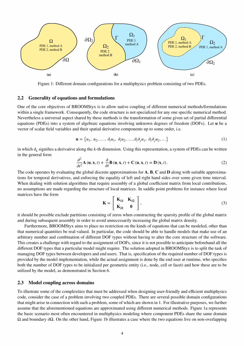
Figure 1: Different domain configurations for a multiphysics problem consisting of two PDEs.

2.2 Generality of equations and formulations

One of the core objectives of BROOMStyx is to allow native coupling of different numerical methods/formulationswithin a single framework. Consequently, the code structure is not specialized for any one specific numerical method.Nevertheless a universal aspect shared by these methods is the transformation of some given set of partial differentialequations (PDEs) into a system of algebraic equations involving unknown degrees of freedom (DOFs). Let u be avector of scalar field variables and their spatial derivative components up to some order, i.e.

u ={u1, u2,… , )iu1, )iu2,… , )i)ju1, )i)ju2,…

} (1)in which )k signifies a derivative along the k-th dimension. Using this representation, a system of PDEs can be writtenin the general form

)2

)t2A (u, x, t) + )

)tB (u, x, t) + C (u, x, t) = D (x, t) . (2)

The code operates by evaluating the global discrete approximations for A, B, C and D along with suitable approxima-tions for temporal derivatives, and enforcing the equality of left and right hand sides over some given time interval.When dealing with solution algorithms that require assembly of a global coefficient matrix from local contributions,no assumptions are made regarding the structure of local matrices. In saddle point problems for instance where localmatrices have the form

K =[K11 K12K21 0

], (3)

it should be possible exclude partitions consisting of zeros when constructing the sparsity profile of the global matrixand during subsequent assembly in order to avoid unnecessarily increasing the global matrix density.

Furthermore, BROOMStyx aims to place no restriction on the kinds of equations that can be modeled, other thanthat numerical quantities be real-valued. In particular, the code should be able to handle models that make use of anarbitrary number and combination of different DOF types without having to alter the core structure of the software.This creates a challenge with regard to the assignment of DOFs, since it is not possible to anticipate beforehand all thedifferent DOF types that a particular model might require. The solution adopted in BROOMStyx is to split the task ofmanaging DOF types between developers and end users. That is, specification of the required number of DOF types isprovided by the model implementation, while the actual assignment is done by the end user at runtime, who specifiesboth the number of DOF types to be initialized per geometric entity (i.e., node, cell or facet) and how these are to beutilized by the model, as demonstrated in Section 6.

2.3 Model coupling across domains

To illustrate some of the complexities that must be addressed when designing user-friendly and efficient multiphysicscode, consider the case of a problem involving two coupled PDEs. There are several possible domain configurationsthat might arise in connection with such a problem, some of which are shown in 1. For illustrative purposes, we furtherassume that the aforementioned equations are approximated using different numerical methods. Figure 1a representsthe basic scenario most often encountered in multiphysics modeling where component PDEs share the same domainΩ and boundary )Ω. On the other hand, Figure 1b illustrates a case where the two equations live on non-overlapping

4

domains that share a common interface, Γ. A classic example of such a scenario occurs in fluid-structure interactionproblems, where Γ acts as a boundary for both Ω1 and Ω2. An additional rule must be specified relating the boundaryconditions of the different PDEs, and depending on modeling choices this can result in either one-way or two-waycoupling of the equations. On the other hand Figure 1c can be understood as an extension of Figure 1a in that one ofthe PDEs is defined over Ω1 ∪ Ω2 and the other over Ω1. Consequently, the latter must have its boundary conditionsdefined on Γ. In contrast, this interface is non-existent with respect to the other equation whose boundary conditionsare defined on )Ω2. In order for the software to be effective, the end user must have the possibility to set up thesedifferent configurations solely via the input file.

2.4 Information access via manager classes

In traditional object-oriented programming, a member object generally does not have access to the methods of itsparent or other objects higher up in the compositional hierarchy. Rigid adherence to this principle means that allinformation needed by a class implementing some particular numerical model must be passed as arguments whencalling a particular class method, which is disadvantageous for two main reasons. First of all, such an approach makesmethod calls extremely long. The same phenomenon is obtained when a user-implemented function is not given accessto other methods/functions within the framework. This is evident for instance in the definition of user-programmedelement (UEL) subroutines in Abaqus, shown below[13]:

1 SUBROUTINE UEL(RHS,AMATRX,SVARS,ENERGY,NDOFEL,NRHS,NSVARS,2 1 PROPS,NPROPS,COORDS,MCRD,NNODE,U,DU,V,A,JTYPE,TIME,DTIME,3 2 KSTEP,KINC,JELEM,PARAMS,NDLOAD,JDLTYP,ADLMAG,PREDEF,NPREDF,4 3 LFLAGS,MLVARX,DDLMAG,MDLOAD,PNEWDT,JPROPS,NJPROP,PERIOD)5 C6 INCLUDE ’ABA_PARAM.INC’7 C8 DIMENSION RHS(MLVARX,*),AMATRX(NDOFEL,NDOFEL),PROPS(*),9 1 SVARS(*),ENERGY(8),COORDS(MCRD,NNODE),U(NDOFEL),

10 2 DU(MLVARX,*),V(NDOFEL),A(NDOFEL),TIME(2),PARAMS(*),11 3 JDLTYP(MDLOAD,*),ADLMAG(MDLOAD,*),DDLMAG(MDLOAD,*),12 4 PREDEF(2,NPREDF,NNODE),LFLAGS(*),JPROPS(*)13 ...14 ...15 RETURN16 END

More importantly, the amount of information accessible to model/algorithm developers becomes hard-coded in thedeclaration of base classes and cannot be subsequently modified without altering each and every derived class alreadycoded. To circumvent this problem, BROOMStyx makes use of manager classes, whose public methods are acces-sible to all objects. While this may seem to break encapsulation, it endows model-implementing classes with almostunlimited flexibility, and at the same time allows them to access only the information that is actually required by themodel at a given instant. In this sense, the software can be viewed as a library/framework hybrid that aims to retainthe benefits of both approaches.

3 Framework architecture

The general structure of the BROOMStyx code is comprised of different class groups as shown in Figure 2. The firstgroup consists of non-polymorphic classes within the broomstyx namespace whose modification/maintenance is leftto the core developers of the framework. These are referred to as core classes, and may further be divided into twosubgroups depending on the number of actual objects that can be instantiated from them at runtime. The rest arepolymorphic classes which deal with different aspects of model and algorithm development, the reading of differentmesh formats and the writing of output.

3.1 Single-instance core classes

Single-instance core classes consist of AnalysisModel, ObjectFactory, and the various manager classes which arecolored blue in Figure 2. AnalysisModel provides two public methods. The first is initializeYourself() whichinstantiates the manager classes, reads the input file and creates all the necessary objects for the simulation throughcalls to the various methods provided by said manager classes. The second is solveYourself() which carries out the

5

1

1..*

0..*1..*

0..*

1

0..*1

1..*

0..*

0..*

1..*

0..*

0..*

1..*

1..*

0..*0..*

1..*

0..*

0..*

0..*

0..*

1..*

AnalysisModel

DofManager

Dof

DomainManager

MeshReader

Node

Cell

NumericsStatus

EvalPoint

MaterialManager

Material

MaterialStatus

NumericsManager

Numerics

IntegrationRule

BasisFunction

SolutionManager

LoadStep

SolutionMethod

LinearSolverSparseMatrix

BoundaryCondition

FieldCondition

InitialCondition

OutputManager

OutputQuantity

OutputWriter

Figure 2: Class diagram showing the general structure of the BROOMStyx code.

actual simulation. To ensure that only a single instance is generated for the entire duration of the program, Analysis-Model is implemented as a Meyers singleton pattern. In addition, the various manager classes have private constructorsand destructors that are accessible to AnalysisModel by virtue of being declared a friend class. Finally, AnalysisModelis responsible for instantiating the proper MeshReader object to read the mesh file supplied by the user.

Among the manager classes, DomainManager is responsible for the management of objects corresponding to thenodes and cells of the mesh, setting up information regarding connectivity, and providing methods for accessing thedegrees of freedom associated with each geometric entity. On the other hand, the creation and deletion of the actualdegrees of freedom are handled by the DofManager class, which also provides methods to set subsystem, group andequation numbers at each DOF, and to update and finalize values for the unknown variables of the simulation. Inaddition, DofManager provides a method for reading multi-freedom constraints from the input file which can then beused to set up constraints involving master/slave DOFs.

The MaterialManager class is responsible for reading the number and types of materials that are declared inthe input file, and for instantiating and initializing the corresponding Material objects. In general, destruction ofmanaged objects is performed when the destructor for their corresponding manager object is invoked; this is true forthe MaterialManager class as well as the subsequent manager classes that will be discussed. Furthermore in theinput file each material must be assigned a unique integer label, and the manager class provides a method to accessinstantiated materials based on their assigned labels. Class NumericsManager is similar to MaterialManager in itsfunction, i.e. it reads the different numerics types specified in the input file together with their assigned integer label,and instantiates the corresponding Numerics objects. Likewise, it provides a method for accessing the instantiatednumerics based on their assigned labels.

The main role of the SolutionManager class is to read the number of load steps from the input file and instantiatethe corresponding LoadStep objects. It also reads all specified initial conditions from the same file, and imposes themat the beginning of the solution process. In addition, it is responsible for instantiating and managing UserFunctionobjects that implement user-programmed functions. Finally, the OutputManager class is in charge of managing allthings related to simulation output. It instantiates a particular OutputWriter object according to the type specifiedby the user in the input file. It also reads the different output quantities that need to be calculated and creates theappropriate OutputQuantity objects. The manager class provides methods for initializing these objects as well as forcalculating and writing output at the end of each converged time step.

Finally, BROOMStyx contains an ObjectFactory class, which as its name implies is in charge of the actual creationof objects based on derived classes. To accomplish this, the framework provides the macro

registerBroomstyxObject(<baseClass>, <derivedClass>)

6

within the broomstyx namespace, which must be invoked in the source code of each derived class. Like Analysis-Model, the ObjectFactory class is implemented as a Meyers singleton and provides two sets of methods. The first setinvolves registration of derived classes that is accessed indirectly via the aforementioned macro, while the second setcreates objects of the different derived class types. The various manager classes instantiate derived objects via a call toObjectFactory which then returns a pointer to the instantiated object, at which point responsibility for the said object istransferred to the calling manager class. At program startup, a map is automatically created within the ObjectFactoryinstance whose key entries are the names of all available derived classes, which are in turn paired with pointers to thecorresponding class constructors.

As mentioned in Section 2, public methods of the manager classes can be accessed anywhere within the broomstyxnamespace and are initiated via a call to the AnalysisModel object which has global scope. For instance, one canretrieve the nodes associated with some particular cell object via the following call:

1 std::vector<Node*> cellNodes = analysisModel().domainManager().giveNodesOf(targetCell);

3.2 Multiple-instance core classes

The subgroup of multiple-instance core classes consist of class types pertaining to geometrical entities and also con-cepts related to the solution process. Class Dof is an abstraction for a single degree of freedom, and it stores datapertaining to which DOF group, solution stage and subsystem it belongs, its equation number, current and convergedvalues of its associated unknown and the corresponding residual value. It also keeps track of its status, i.e., whether itis constrained (and if so, the value of the constraint) and in the case that it is of slave type, the pointer to its associatedmaster DOF. The class itself does not provide any methods for accessing its members, which are all declared private.Instead their retrieval and update is done through DofManager that is declared a friend class of Dof. Meanwhile, theNode class is an abstraction for a geometric entity, specifically a point in 3-dimensional space. It stores the point’scoordinates, a unique ID number, a vector of pointers to Dof objects that live on the node, and a vector of real numberswhose length is set by the end user at runtime and which serves to store values that will subsequently be written intooutput files. Furthermore it contains two sets of pointers to Cell objects that are attached to the node, one for domaincells and the other for boundary cells.

The Cell class on the other hand has a more nuanced function. Rather than simply being an abstraction for a partic-ular geometric entity, its primary purpose is to act as an anchor to which Numerics objects can attach their associateddata and perform the necessary calculations related to the governing equations. Every Cell object contains a vector ofreal numbers, the length of which is set at runtime in order to store values needed for writing output similar to the caseof the Node class. Each Cell object also stores its own type (e.g., 3-node triangle, 10-node tetrahedron, general n-pointpolygon) and dimension, its ID number, physical entity, and a vector of pointers to Dof objects associated with thecell. In addition it stores data related to connectivity, such as its neighbors and faces. Every Cell instance also containsa vector of pointers to Node objects, whose exact relation to the cell may vary depending on the particular formulationbeing used. For instance within the context of a standard finite difference scheme each cell may be associated to someFD stencil so that the cell nodes are meant to coincide with the stencil points, whereas in a finite element schemethe Cell object can be seen as representing a single element, and the nodes as entities to which shape functions areassociated in order to approximate a piecewise solution. Cell objects are also used to represent geometrical entitiessuch as surfaces on which boundary and interface conditions are applied. Lastly, when cell faces are required to beconstructed by a particular formulation, these are also represented as Cell objects. For this reason the DomainMan-ager class distinguishes between three types of cells: a) domain cells that are associated with some given Numericsinstance1, b) boundary cells that are associated some particular boundary condition, and c) face cells.

The EvalPoint class is an abstraction for a single evaluation point. It stores the coordinates of its location in additionto its assigned weight (in the case of Gauss integration), and contains a pointer to a NumericsStatus object that in turnstores data such as history variables required by Numerics and Material objects for performing their calculations. Asshown in Figure 2, EvalPoint objects typically occur as components of some NumericsStatus instance. Nonethelesstheir existence is not mandatory; cells which have only one evaluation point for example can have the necessarynumerics and material variables stored directly as members of the immediate NumericsStatus object connected to thecell instance, thus avoiding compositions of the type Cell->NumericsStatus->EvalPoint->NumericsStatus.

1This group may also include lower-dimensional interface cells, for example when the latter are associated with a Numerics object imple-menting some inter-domain or multiphysics coupling.

7

Table 1: General solution procedure executed on invocation of LoadStep->solveYourself().

1. Initialize solvers to be used by solution methods.2. Carry out pre-processing routines.3. Find constrained and active degrees of freedom.4. Determine target time for current substep. If this exceeds the specified end time,

shorten it so that the target time exactly coincides with the end time.5. For each solution stage, have the corresponding SolutionMethod object calculate

the solution given the specified boundary and field conditions.6. If solution in step 5 converged, finalize the relevant data. Otherwise, implement

contingency procedures (e.g., change the time-increment and go back to step 4, oralternatively terminate the simulation due to unconverged results.)

7. Update current time and possibly also the time increment (adaptive time stepping).If end time has been reached, then proceed to step 8. Otherwise, go back to step 4.

8. Carry out post-processing routines.

The BoundaryCondition class is used to store information regarding a single boundary condition, such as thephysical entity label corresponding to the boundary on which the condition is to be applied, the particular BC type, thetarget Dof type and the implementing numerics. This last piece of information is necessary since a BoundaryConditionobject is not in charge of actually imposing its given BC. Rather, said object calculates the value (possibly time-dependent) of the relevant quantity at the required location on the boundary and leaves the imposition of this value tothe implementing Numerics object.2 The FieldCondition and InitialCondition classes are have similar function —the former is used to describe domain-wide quantities, for example specific source terms and possibly also parametersof governing equations that are made to vary in space and time, whereas the latter returns the value of a specific initialcondition at some given location within the domain. As with BoundaryCondition, the actual implementations of thesefield and initial conditions are left to the respective associated Numerics objects.

Class LoadStep is an abstraction for a solution step taken over a range of time, which in turn can be further dividedinto substeps. Essentially the workhorse class of the entire code, LoadStep objects are responsible for marching thesolution forward in time according parameters specified by the end user. Each LoadStep object reads its required datafrom the input file; these consist of the starting time and ending time of the solution step, the initial time increment foreach substep, the maximum allowed number of substeps, all the boundary and field conditions to be imposed for thecurrent solution step, the particular type of solution method to be used, and all special pre-/post-processing proceduresavailable in numerics implementations that are required to be performed according to end user specifications. TheLoadStep class provides the method solveYourself(), which carries out the sequence procedures listed in Table1. Note that steps 2 and 8, pre- and post-processing do not refer to meshing/visualization procedures as commonlyunderstood in FEM terminology, but instead denote access points built into the framework which can be exploited bymodel developers to perform calculations that are not meant for execution during assembly and solution of systemequations, for instance the initialization of some history variables based on the latest converged solution.

3.3 Polymorphic classes

The BROOMStyx framework contains several polymorphic classes that can be used to extend functionality of thesoftware. As illustrated in Figure 2, these fall into four groups. The first group is composed of the MeshReader classand deals with the interpretation of mesh files generated from third party software and the creation of the correspondingentities in the internal memory of the software. Meanwhile, the second group is concerned with model creation, andconsists of the Numerics, Material, ShapeFunction and IntegrationRule classes. The third group allows for theimplementation of different solution schemes and back-end solvers, and includes the SolutionMethod, LinearSolverand SparseMatrix classes. The last group allows the production of different output formats and the calculation of

2The main reason for adopting such a strategy is that numerical methods generally differ in the way they impose boundary conditions.For instance some schemes such as the Element-Free Galerkin method[8] make use of shape functions that do not possess Kronecker-deltaproperties, hence Dirichlet conditions must be imposed differently compared to finite element schemes even if both are based on a variationalformulation of the governing equations. Passing on the actual implementation of boundary conditions and the like to the specific numericsallows us to avoid having to overload BoundaryCondition for each new Numerics derived class.

8

specialized quantities through the classes OutputWriter and OutputQuantity.

3.3.1 MeshReader

The MeshReader class provides a way for the BROOMStyx framework to understand output files from external CADand mesh generation tools which contain the discretization (i.e. nodes and elements) to be used in the numericalsimulation. At present, the framework allows for the instantiation of one MeshReader-derived object that reads asingle mesh file containing all the necessary components of the discretization, whose name is specified in the inputfile. At the same time, said MeshReader object interfaces with the DomainManager object to create the resultinggeometric entities in memory.

3.3.2 Numerics

The Numerics class is an abstraction for a PDE (or system of PDEs) together with its numerical discretization, and isthe fundamental building block around which the rest of the code was designed. It contains methods for calculatinglocal contributions corresponding to different components of the governing equations as described in Section 2. Itsderived classes are responsible for declaring the required geometric cell type to be used with said class and the numberof DOFs that will be utilized at each node, cell or face. The base class declaration is given in Listing 1, where for brevityonly the virtual methods are listed. Each instantiated Numerics object reads its required parameters from the inputfile, and manages its own data at each computational cell. Because different physical processes vary in the amountand types of data that they require to be stored, an auxiliary class NumericsStatus is provided whose role is to be abase container that can be specialized to suit the various Numerics-derived classes. Each computational cell includesa pointer to one NumericsStatus object in its attributes, which is instantiated by the Numerics object assigned to thecell when data storage beyond standard DOF solutions is required. As can be seen from Listing 1, the class containsmethods for calculating output quantities, and for performing pre-/postprocessing of data as well as carrying out inter-iteration operations. This is to allow a maximum amount of flexibility to developers, since in BROOMStyx flow ofcontrol does not rest with any instantiated Numerics object but rather with the framework itself that in turn passes it tothe specific solution method chosen by the end user at runtime. During assembly of the discrete equations, the lattercycles over all cells in the computational domain and interfaces directly with the Numerics object assigned to each cell,meaning that entities such as integration points are hidden from solution algorithms. This is a deliberate design choice,since the notion of integration points does not always make sense, for example when dealing with finite differences orcontrol volume schemes. Hence for numerical methods based on weak formulations, the Numerics object itself is incharge of internally performing the numerical integration when calculating local matrices and vectors.

The convention adopted in BROOMStyx for stating method declarations is to clearly separate input arguments fromoutput quantities, except when a particular variable acts as both input and output. Multiple return values are passed as atuple, for instance in methods that return local matrix and vector contributions. As can be observed in Listing 1, matrixoutput is returned using something akin to coordinate (COO) format, i.e. as a collection of three vectors, the first twocontaining pointers to Dof objects which store their equation numbers (corresponding respectively to row and columnindices in the global coefficient matrix) while the last vector contains the actual entries of the matrix. A key advantageof such an approach is that no assumption is made on the shape of such matrix, but rather that the method only returnslocal components that are actually nonzero. This is important in terms of efficiency, since the sparsity profiles forglobal coefficient matrices are determined by an initial assembly process that disregards local matrix values.

The following two details are worth mentioning with regard to interface design:a) The virtual methods defined in the Numerics base class for calculating matrix and vector quantities corresponding

to different components of governing equations are not pure virtual methods but rather are implemented in the baseclass as empty functions. For example, transient ()∕)t) terms may be calculated with the following two methods:

1 virtual std::tuple< std::vector<Dof*>, std::vector<Dof*>, RealVector >2 giveTransientCoefficientMatrixAt(Cell* targetCell, int stage, int subsys, const TimeData& time);34 virtual std::tuple< std::vector<Dof*>, RealVector >5 giveTransientLeftHandSideAt(Cell* targetCell, int stage, int subsys, const TimeData& time, ValueType valType);

The existence of an empty implementation in the base class means that developers only need to override methodsthat are actually relevant to the problem at hand. This reduces the amount of boilerplate code the must be written

9

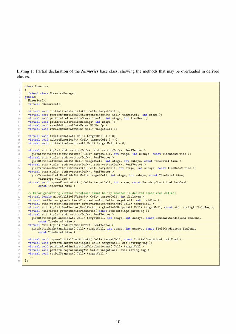
Listing 1: Partial declaration of the Numerics base class, showing the methods that may be overloaded in derivedclasses.

1 class Numerics2 {3 friend class NumericsManager;4 public:5 Numerics();6 virtual ~Numerics();7 ...8 virtual void initializeMaterialsAt( Cell* targetCell );9 virtual bool performAdditionalConvergenceCheckAt( Cell* targetCell, int stage );

10 virtual void performPreIterationOperationsAt( int stage, int iterNum );11 virtual void printPostIterationMessage( int stage );12 virtual void readAdditionalDataFrom( FILE* fp );13 virtual void removeConstraintsOn( Cell* targetCell );1415 virtual void finalizeDataAt( Cell* targetCell ) = 0;16 virtual void deleteNumericsAt( Cell* targetCell ) = 0;17 virtual void initializeNumericsAt( Cell* targetCell ) = 0;1819 virtual std::tuple< std::vector<Dof*>, std::vector<Dof*>, RealVector >20 giveStaticCoefficientMatrixAt( Cell* targetCell, int stage, int subsys, const TimeData& time );21 virtual std::tuple< std::vector<Dof*>, RealVector >22 giveStaticLeftHandSideAt( Cell* targetCell, int stage, int subsys, const TimeData& time );23 virtual std::tuple< std::vector<Dof*>, std::vector<Dof*>, RealVector >24 giveTransientCoefficientMatrixAt( Cell* targetCell, int stage, int subsys, const TimeData& time );25 virtual std::tuple< std::vector<Dof*>, RealVector >26 giveTransientLeftHandSideAt( Cell* targetCell, int stage, int subsys, const TimeData& time,27 ValueType valType );28 virtual void imposeConstraintAt( Cell* targetCell, int stage, const BoundaryCondition& bndCond,29 const TimeData& time );3031 // Error-generating virtual functions (must be implemented in derived class when called)32 virtual double giveCellFieldValueAt( Cell* targetCell, int fieldNum );33 virtual RealVector giveCellNodeFieldValuesAt( Cell* targetCell, int fieldNum );34 virtual std::vector<RealVector> giveEvaluationPointsFor( Cell* targetCell );35 virtual std::tuple< RealVector,RealVector > giveFieldOutputAt( Cell* targetCell, const std::string& fieldTag );36 virtual RealVector giveNumericsParameter( const std::string& paramTag );37 virtual std::tuple< std::vector<Dof*>, RealVector >38 giveStaticRightHandSideAt( Cell* targetCell, int stage, int subsys, const BoundaryCondition& bndCond,39 const TimeData& time );40 virtual std::tuple< std::vector<Dof*>, RealVector >41 giveStaticRightHandSideAt( Cell* targetCell, int stage, int subsys, const FieldCondition& fldCond,42 const TimeData& time );4344 virtual void imposeInitialConditionAt( Cell* targetCell, const InitialCondition& initCond );45 virtual void performPostprocessingAt( Cell* targetCell, std::string tag );46 virtual void performPrefinalizationCalculationsAt( Cell* targetCell );47 virtual void performPreprocessingAt( Cell* targetCell, std::string tag );48 virtual void setDofStagesAt( Cell* targetCell );49 ...50 };

10

Listing 2: Declarations for MaterialStatus and Material classes.1 class Material2 {3 public:4 Material();5 virtual ~Material();67 virtual MaterialStatus* createMaterialStatus();8 virtual void destroy( MaterialStatus*& matStatus );9 virtual void initialize();

10 virtual void readParamatersFrom( FILE* fp );11 virtual void updateStatusFrom( const RealVector& conState, MaterialStatus* matStatus );12 virtual void updateStatusFrom( const RealVector& conState, MaterialStatus* matStatus,13 const std::string& label );1415 // Error-generating virtual methods (must be implemented in derived class when called)16 virtual double givePotentialFrom( const RealVector& conState, const MaterialStatus* matStatus );17 virtual RealVector giveForceFrom( const RealVector& conState, const MaterialStatus* matStatus );18 virtual RealVector giveForceFrom( const RealVector& conState, const MaterialStatus* matStatus,19 const std::string& label );20 virtual RealMatrix giveModulusFrom( const RealVector& conState, const MaterialStatus* matStatus );21 virtual RealMatrix giveModulusFrom( const RealVector& conState, const MaterialStatus* matStatus,22 const std::string& label );23 virtual double giveMaterialVariable( const std::string& label, const MaterialStatus* matStatus );24 virtual double giveParameter( const std::string& label );2526 protected:27 std::string _name;28 void error_unimplemented( const std::string& method );29 };

and also ensures that static equations are correctly solved when using solution methods that account for transientterms. Such functionality is necessary due to the fact that one can have a fully coupled system that features bothstatic and time-varying PDEs.

b) The return values for the above methods are in the form of tuples, which must be constructed utilizing bothstd::make tuple(...) and std::move in order to avoid unwanted copying, e.g.

1 std::vector<Dof*> rowDof, colDof;2 RealVector coefVal;3 ...4 return std::make_tuple(std::move(rowDof), std::move(colDof), std::move(coefVal));

3.3.3 Material

Class Material represents the base class for constitutive models, whose role is to evaluate quantities that determinethe coefficients/parameters of the governing equations. It provides methods to calculate scalar potentials, constitutiveforces and tangent moduli. The class interface design is shown in Listing 2, and is based on the concept of a scalarpotential function and its derivatives. That is, we assume that the material model can be described by some scalarpotential

f = f (�,�) (material potential) (4)whose value can be computed give the current constitutive state � and set of history variables�. Likewise, it is assumedthat its gradients with respect to the constitutive state variables may also be obtained as

� = ))�f (�,�) (material force) (5)

D = ))�� (�,�) (material modulus) (6)

Subsequently, lines 16–22 in Listing 2 are abstractions for the calculations needed to obtain the expressions givenabove, and are declared virtual as they are to be overridden in derived class definitions. In general however, materialmodels do not necessarily have the well defined structure implied by (4)–(6), and the framework does not require that

11

Listing 3: Definition of the SolutionMethod class.1 class SolutionMethod2 {3 public:4 SolutionMethod();5 virtual ~SolutionMethod();67 void getCurrentLoadStep();8 void imposeConstraintsAt( int stage, const std::vector<BoundaryCondition>& bndCond, const TimeData& time );9

10 virtual int computeSolutionFor( int stage11 , const std::vector<BoundaryCondition>& bndCond12 , const std::vector<FieldCondition>& fldCond13 , const TimeData& time ) = 0;1415 virtual void formSparsityProfileForStage( int stage ) = 0;16 virtual void initializeSolvers() = 0;17 virtual void readDataFromFile( FILE* fp ) = 0;1819 protected:20 LoadStep* _loadStep;21 std::string _name;2223 bool checkConvergenceOfNumericsAt( int stage );24 };

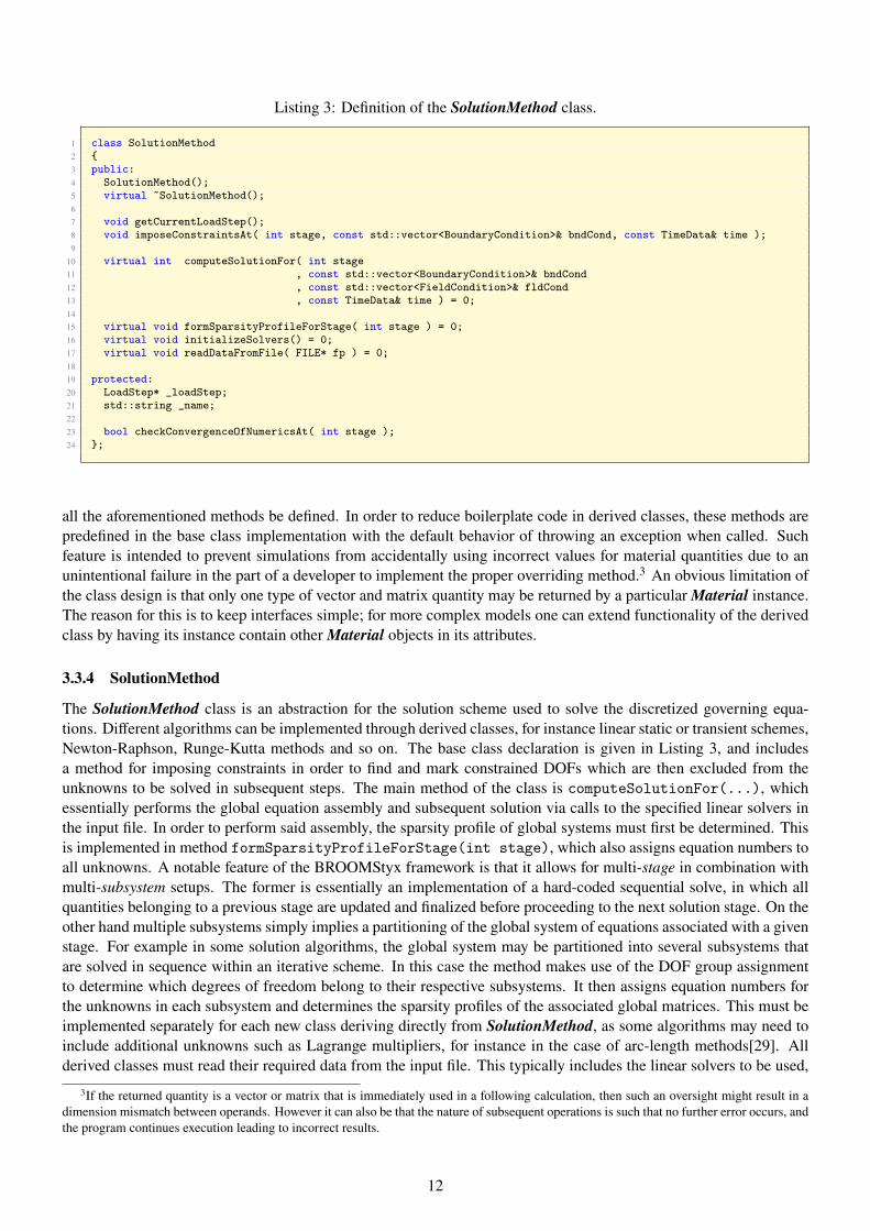
all the aforementioned methods be defined. In order to reduce boilerplate code in derived classes, these methods arepredefined in the base class implementation with the default behavior of throwing an exception when called. Suchfeature is intended to prevent simulations from accidentally using incorrect values for material quantities due to anunintentional failure in the part of a developer to implement the proper overriding method.3 An obvious limitation ofthe class design is that only one type of vector and matrix quantity may be returned by a particular Material instance.The reason for this is to keep interfaces simple; for more complex models one can extend functionality of the derivedclass by having its instance contain other Material objects in its attributes.

3.3.4 SolutionMethod

The SolutionMethod class is an abstraction for the solution scheme used to solve the discretized governing equa-tions. Different algorithms can be implemented through derived classes, for instance linear static or transient schemes,Newton-Raphson, Runge-Kutta methods and so on. The base class declaration is given in Listing 3, and includesa method for imposing constraints in order to find and mark constrained DOFs which are then excluded from theunknowns to be solved in subsequent steps. The main method of the class is computeSolutionFor(...), whichessentially performs the global equation assembly and subsequent solution via calls to the specified linear solvers inthe input file. In order to perform said assembly, the sparsity profile of global systems must first be determined. Thisis implemented in method formSparsityProfileForStage(int stage), which also assigns equation numbers toall unknowns. A notable feature of the BROOMStyx framework is that it allows for multi-stage in combination withmulti-subsystem setups. The former is essentially an implementation of a hard-coded sequential solve, in which allquantities belonging to a previous stage are updated and finalized before proceeding to the next solution stage. On theother hand multiple subsystems simply implies a partitioning of the global system of equations associated with a givenstage. For example in some solution algorithms, the global system may be partitioned into several subsystems thatare solved in sequence within an iterative scheme. In this case the method makes use of the DOF group assignmentto determine which degrees of freedom belong to their respective subsystems. It then assigns equation numbers forthe unknowns in each subsystem and determines the sparsity profiles of the associated global matrices. This must beimplemented separately for each new class deriving directly from SolutionMethod, as some algorithms may need toinclude additional unknowns such as Lagrange multipliers, for instance in the case of arc-length methods[29]. Allderived classes must read their required data from the input file. This typically includes the linear solvers to be used,

3If the returned quantity is a vector or matrix that is immediately used in a following calculation, then such an oversight might result in adimension mismatch between operands. However it can also be that the nature of subsequent operations is such that no further error occurs, andthe program continues execution leading to incorrect results.

12

Listing 4: Definitions for the SparseMatrix and LinearSolver classes.1 class SparseMatrix2 {3 public:4 SparseMatrix();5 virtual ~SparseMatrix();67 std::tuple< int,int > giveMatrixDimensions();8 int giveNumberOfNonzeros();9 bool isSymmetric();

10 void setSymmetryTo( bool true_or_false );1112 virtual void addToComponent( int rowNum, int colNum, double val ) = 0;13 virtual void atomicAddToComponent( int rowNum, int colNum, double val ) = 0;14 virtual void finalizeProfile() = 0;15 virtual std::tuple< int*,int* > giveProfileArrays() = 0;16 virtual double* giveValArray() = 0;17 virtual void insertNonzeroComponentAt( int rowIdx, int colIdx ) = 0;18 virtual void initializeProfile( int dim1, int dim2 ) = 0;19 virtual void initializeValues() = 0;20 virtual RealVector lumpRows() = 0;21 virtual void printTo( FILE* fp, int n ) = 0;22 virtual RealVector times( const RealVector& x ) = 0;2324 protected:25 int _dim1;26 int _dim2;27 int _nnz;28 bool _symFlag;29 };3031 class LinearSolver32 {33 public:34 LinearSolver();35 virtual ~LinearSolver();3637 virtual void allocateInternalMemoryFor( SparseMatrix* coefMat );38 virtual RealVector backSubstitute( SparseMatrix* coefMat, RealVector& rhs );39 virtual void factorize( SparseMatrix* coefMat );40 virtual bool giveSymmetryOption();41 virtual void initialize();42 virtual void clearInternalMemory();43 virtual void setInitialGuessTo( RealVector& initGuess );44 virtual bool takesInitialGuess();4546 virtual std::string giveRequiredMatrixFormat() = 0;47 virtual void readDataFrom( FILE* fp ) = 0;48 virtual RealVector solve( SparseMatrix* coefMat, RealVector& rhs ) = 0;49 };

convergence criteria for each of the active DOF groups in the case of nonlinear solution schemes, and data related tospecial procedures such as line search options when these are implemented in the derived class.

3.3.5 LinearSolver and SparseMatrix

BROOMStyx relies on external software packages for the solution of linear systems. Class LinearSolver is a base classfor wrappers to different solver libraries in order to provide a common interface that can be utilized by other classeswithin BROOMStyx. The base class declaration is given in Listing 4, and contains a varied number of methodsthat are relevant for either direct or iterative solvers. Derived classes must be able to specify the format of globalcoefficient matrices to be used during assembly of equations, read all data required by the back-end solver such astolerances, and also perform the solution of a given linear system by internally making the necessary calls to the actualsolver. At present, BROOMStyx can interface with different versions of the direct solver PARDISO[35, 1] as wellas iterative solvers from the ViennaCL library[31] compiled to run on graphics processors via CUDA. Meanwhile,the SparseMatrix class is used to accommodate different matrix formats that may be utilized by the various linearsolver packages, such as compressed sparse row (CSR) and coordinate (COO) formats. In order to allocate memoryfor a given spare matrix, its sparsity profile must first be determined. The class method initializeProfile(int

13

m, int n) is used to specify the matrix dimensions, and also resets its nonzero components to the empty set. Onthe other hand, the method insertNonzeroComponentAt(int i, int j) declares the (i, j)-th component of thematrix to be nonzero. The sparsity profile of the global matrix can then be constructed by constructing the localcontributions from each cell and then calling the aforementioned method for each nonzero matrix component in thelocal contribution, with its corresponding global indices as arguments. Finally, finalizeProfile() constructs theactual arrays for storing location indices and values according to the specified matrix format.

3.3.6 OutputWriter and OutputQuantity

The primary function of the OutputWriter class is to create output files containing user-chosen simulation results atcertain points in time as specified in the input file. These normally consist of the values for primary unknowns at nodesor elements, as well as physical variables such as stresses, strains and so on. In general, OutputWriter objects onlyhave access to values specified in connection with the NodalField and CellFieldOutput keywords in the inputfile. Derived classes are in charge of writing said output files in a format that can be read by third party visualizationpackages. The specific details on what to include in these files is read by the OutputWriter instance from the input file,while the frequency of creating output files relative to the start and end times of the simulation is read by LoadStepobjects as part of their required data.

On the other hand, the OutputQuantity class enables retrieval of specialized data during the course of simulationsthat are not normally found in the output files described above. Examples are force reactions pertaining to a particularportion of the external boundary, and results of special procedures such as J -integral[28] calculations. In addition,derived classes may be used to implement integration of particular quantities over the problem domain (e.g. in orderto calculate global error norms), or to set up “observation points” to track the evolution of specific quantities at auser-selected location.

4 Vector and matrix operations

For numerical schemes such as finite and boundary elements, a substantial portion of the total running time for a givensimulation is spent on dense matrix and vector operations. It is therefore important that such calculations are performedefficiently, and in BROOMStyx this is be done by making use of specialized BLAS implementations such as MKL[1]or OpenBLAS[39]. Unfortunately, the interfaces provided by BLAS can be rather intimidating for those not well-versed in their usage. Consider for example the BLAS function dgemv that is used for matrix-vector multiplicationwith double floating point entries. It performs the operation y ∶= �op (A) x + �y for op (A) = A or AT and has thefollowing declaration:

1 void cblas_dgemv(const CBLAS_LAYOUT Layout, const CBLAS_TRANSPOSE TransA, const MKL_INT M, const MKL_INT N,const double alpha, const double *A, const MKL_INT lda, const double *X, const MKL_INT incX, const doublebeta, double *Y, const MKL_INT incY);

In order to provide a more user-friendly environment for developers, BROOMStyx provides RealVector and Real-Matrix classes as abstractions for dense vectors and matrices of real (type double) numbers, the latter storing theircomponents in column-major format. Accordingly, the +,-,* and / operators are overloaded to accept matrix and vectorarguments. They function as high-level wrappers that call appropriate BLAS routines to perform the actual matrix op-erations. In addition, they distinguish between lvalue and rvalue operands in order to minimize the occurrence of deepcopies associated with temporary objects. The main purpose is to allow the coding of sequences of matrix and vectoroperations in a way that mimics standard mathematical notation but at the same time results in efficient evaluation.For instance given scalars � and �, matrix A of size n × m and vectors b and c of length n and m respectively, theexpression

d = �ATb + �c (7)can be coded as shown in Listing 5, with the back-end evaluation making use of the BLAS functions dscal, dgemvand daxpy. As operator overloading involves static polymorphism, no run-time overhead is incurred due to virtualfunction calls. Nevertheless, a naive implementation of the operator overloading results in an inefficient calculationas the binary nature of the aforementioned operators prevents us from taking full advantage of the low level BLASfunctions’ capabilities. Such implementation would yield for instance the sequence of operations shown in Table 2.These operations must preserve the original input arguments �, �, A, b and c. Accounting for the move assignment in

14

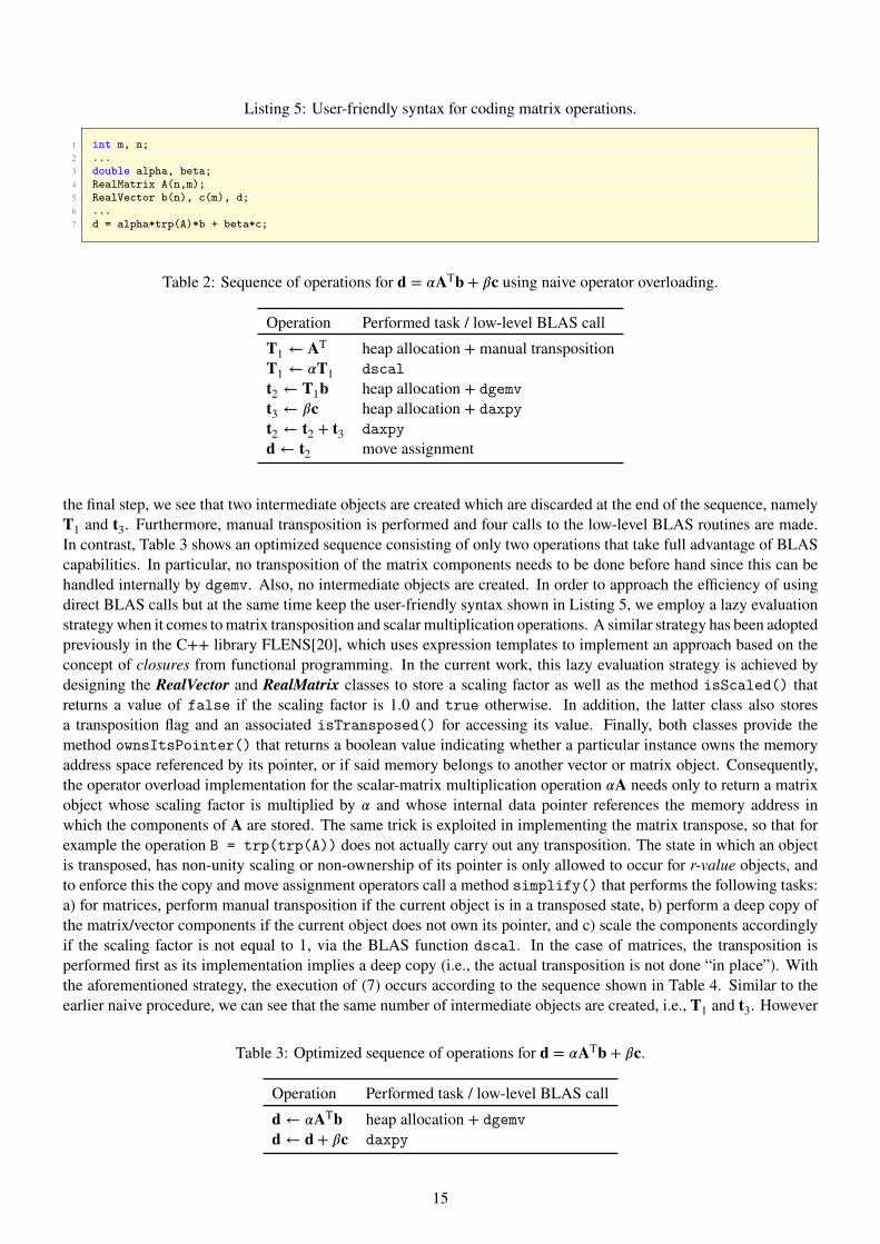
Listing 5: User-friendly syntax for coding matrix operations.1 int m, n;2 ...3 double alpha, beta;4 RealMatrix A(n,m);5 RealVector b(n), c(m), d;6 ...7 d = alpha*trp(A)*b + beta*c;

Table 2: Sequence of operations for d = �ATb + �c using naive operator overloading.

Operation Performed task / low-level BLAS callT1 ← AT heap allocation + manual transpositionT1 ← �T1 dscal

t2 ← T1b heap allocation + dgemv

t3 ← �c heap allocation + daxpy

t2 ← t2 + t3 daxpy

d← t2 move assignment

the final step, we see that two intermediate objects are created which are discarded at the end of the sequence, namelyT1 and t3. Furthermore, manual transposition is performed and four calls to the low-level BLAS routines are made.In contrast, Table 3 shows an optimized sequence consisting of only two operations that take full advantage of BLAScapabilities. In particular, no transposition of the matrix components needs to be done before hand since this can behandled internally by dgemv. Also, no intermediate objects are created. In order to approach the efficiency of usingdirect BLAS calls but at the same time keep the user-friendly syntax shown in Listing 5, we employ a lazy evaluationstrategy when it comes to matrix transposition and scalar multiplication operations. A similar strategy has been adoptedpreviously in the C++ library FLENS[20], which uses expression templates to implement an approach based on theconcept of closures from functional programming. In the current work, this lazy evaluation strategy is achieved bydesigning the RealVector and RealMatrix classes to store a scaling factor as well as the method isScaled() thatreturns a value of false if the scaling factor is 1.0 and true otherwise. In addition, the latter class also storesa transposition flag and an associated isTransposed() for accessing its value. Finally, both classes provide themethod ownsItsPointer() that returns a boolean value indicating whether a particular instance owns the memoryaddress space referenced by its pointer, or if said memory belongs to another vector or matrix object. Consequently,the operator overload implementation for the scalar-matrix multiplication operation �A needs only to return a matrixobject whose scaling factor is multiplied by � and whose internal data pointer references the memory address inwhich the components of A are stored. The same trick is exploited in implementing the matrix transpose, so that forexample the operation B = trp(trp(A)) does not actually carry out any transposition. The state in which an objectis transposed, has non-unity scaling or non-ownership of its pointer is only allowed to occur for r-value objects, andto enforce this the copy and move assignment operators call a method simplify() that performs the following tasks:a) for matrices, perform manual transposition if the current object is in a transposed state, b) perform a deep copy ofthe matrix/vector components if the current object does not own its pointer, and c) scale the components accordinglyif the scaling factor is not equal to 1, via the BLAS function dscal. In the case of matrices, the transposition isperformed first as its implementation implies a deep copy (i.e., the actual transposition is not done “in place”). Withthe aforementioned strategy, the execution of (7) occurs according to the sequence shown in Table 4. Similar to theearlier naive procedure, we can see that the same number of intermediate objects are created, i.e., T1 and t3. However

Table 3: Optimized sequence of operations for d = �ATb + �c.

Operation Performed task / low-level BLAS calld← �ATb heap allocation + dgemv

d← d + �c daxpy

15

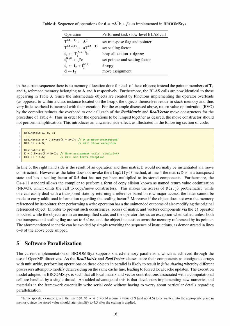
Table 4: Sequence of operations for d = �ATb + �c as implemented in BROOMStyx.

Operation Performed task / low-level BLAS callT(A,1,T)1 ← AT set transpose flag and pointerT(A,�,T)1 ← �T(A,1,T)1 set scaling factort2 ← T(A,�,T)1 b heap allocation + dgemv

t(c,�)3 ← �c set pointer and scaling factort2 ← t2 + t

(c,�)3 daxpy

d← t2 move assignment

in the current sequence there is no memory allocation done for each of these objects; instead the pointer members ofT1and t3 reference memory belonging to A and b respectively. Furthermore, the BLAS calls are now identical to thoseappearing in Table 3. Since the intermediate objects are created by functions implementing the operator overloads(as opposed to within a class instance located on the heap), the objects themselves reside in stack memory and thusvery little overhead is incurred with their creation. For the example discussed above, return value optimization (RVO)by the compiler reduces the overhead to one call each of the RealMatrix and RealVector move constructors for theprocedure of Table 4. Thus in order for the operations to be lumped together as desired, the move constructor shouldnot perform simplification. This introduces an unwanted side effect, as illustrated in the following section of code:

1 RealMatrix A, B, C;2 ...3 RealMatrix D = 0.5*trp(A + B*C); // D is move-constructed4 D(0,0) = 4.5; // will throw exception56 RealMatrix E;7 E = 0.5*trp(A + B*C); // Move assignment calls .simplify()8 E(0,0) = 4.5; // will not throw exception

In line 3, the right hand side is the result of an operation and thus matrix D would normally be instantiated via moveconstruction. However as the latter does not invoke the simplify() method, at line 4 the matrix D is in a transposedstate and has a scaling factor of 0.5 that has not yet been multiplied to its stored components. Furthermore, theC++11 standard allows the compiler to perform a form of copy elision known as named return value optimization(NRVO), which omits the call to copy/move constructors. This makes the access of D(i,j) problematic: whileone can easily deal with a transposed state by returning a reference based on row-major access, the latter cannot bemade to carry additional information regarding the scaling factor.4 Moreover if the object does not own the memoryreferenced by its pointer, then performing a write operation has a the unintended outcome of also modifying the originalreferenced object. In order to prevent such occurrences, access of matrix and vectors components via the () operatoris locked while the objects are in an unsimplified state, and the operator throws an exception when called unless boththe transpose and scaling flag are set to false, and the object in question owns the memory referenced by its pointer.The aforementioned scenario can be avoided by simply rewriting the sequence of instructions, as demonstrated in lines6–8 of the above code snippet.

5 Software Parallelization

The current implementation of BROOMStyx supports shared-memory parallelism, which is achieved through theuse of OpenMP directives. As the RealMatrix and RealVector classes store their components as contiguous arrayswith unit stride, performing operations on these objects in parallel is likely to result in false sharing whereby differentprocessors attempt to modify data residing on the same cache line, leading to forced local cache updates. The executionmodel adopted in BROOMStyx is such that all local matrix and vector contributions associated with a computationalcell are handled by a single thread. An added advantage of this is that developers implementing new numerics andmaterials in the framework essentially write serial code without having to worry about particular details regardingparallelization.

4In the specific example given, the line D(0,0) = 4.5 would require a value of 9 (and not 4.5) to be written into the appropriate place inmemory, since the stored value should later simplify to 4.5 after the scaling is applied.

16

It is common for OpenMP-accelerated software to have code regions that run serially interspersed between blocksthat are executed in parallel. A common example of this is when the software has to perform I/O operations, althoughthis can also be made to run such that a single thread executes write operations to disk while the remaining threadsare already running calculations pertaining to the subsequent time step. While such procedure has not yet been imple-mented in BROOMStyx, we consider this a minor drawback since for heavily nonlinear problems that require a largenumber of iterations, the time spent doing computation far outweighs the amount of time it takes to perform serialwriting of output. Nevertheless, it is beneficial to reduce the amount of time in which the software is running serialcode in order to fully benefit from the multi-core architecture of present day CPUs. To this end, assembly of globalmatrices and vectors is done in parallel, and makes use of atomic operations to avoid data race conditions. On the otherhand, solution of the resulting linear system is done via calls to third-party solvers. Consider for example the directsolver PARDISO, which implements a solution of the linear system based on a sparse LU decomposition of the globalcoefficient matrix. An advantage of direct solvers is that one does not need to provide preconditioners that are oftennecessary to accelerate iterative schemes, and which may be difficult to construct for general nonlinear systems. Theirdrawback is that the cost of the LU decomposition becomes prohibitive for very large problem sizes. The PARDISOinterface allows for splitting of the solution procedure into four phases:a) Reordering, symbolic factorization and allocation of memory to be used by the solverb) numerical factorizationc) forward and back-substitutiond) Release of allocated memoryThe first step is the most costly, taking up to 75% of the total solve time and is also not easily executed in parallel. Manyproblems of interest however can be solved without performing adaptive refinement of the initial spatial discretization,which means that the sparsity profile of the global coefficient matrix does not change over time. Nonlinear solutionalgorithms implemented in BROOMStyx exploit this property by performing symbolic factorization only at the be-ginning iteration of a substep, and then skipping this step in subsequent iterations along with the release of memoryunless the solver returns an error, in which case the stalled solution is restarted going through all the phases listedabove. We have found that when low order methods are employed for the discrete problem, use of the above strategycan reduce the total time for each iteration (i.e., assembly + solve) by as much as 50%.

6 Example applications

In this section, we present several numerical examples dealing on different topics and that are specifically chosen tohighlights important capabilities of the BROOMStyx framework. We note that while all presented examples are in2D, the code structure itself readily admits formulations in both lower and higher dimensions. The first example dealswith torsion and shows the code’s capability to deal with higher order mappings and formulations as well as non-standard degrees of freedom that are not associated with specific geometric entities. The next two examples feature amonolithic coupling of variational and control volume formulations applied to the problem of poroelasticity. The finalexample deals with brittle fracture propagation in concrete using the phase-field approach, which gives rise to a couplednonlinear system of PDEs that must be solved alternately with a Newton approach applied to the inner iterations. Forall problems, discretization of the problem domain was performed using the Gmsh software[16], while 2D color plotswere generated either Paraview and Gmsh, the latter used for higher order visualization.

6.1 Elastic torsion of composite shafts

The Saint-Venant torsion problem is concerned with determining the shear stresses induced in a non-circular prismaticshaft that is rigidly clamped at one end and subjected to an applied torque at the other. This problem has been exten-sively studied in the literature, and a discussion of solution approaches can be found in classic texts such as Fung[15].Numerical solutions are generally designed based on Saint-Venant’s original approach of using a warping function, oralternatively on the Prandtl stress function. Both lead to Laplace/Poisson type governing equations but with notabledifferences in the resulting boundary conditions and constraints. In this example we make use of the former strategy,its chief advantage being that no special treatment is needed when dealing with multiply connected sections.

We begin by considering a prismatic shaft in Cartesian space, whose longitudinal axis is aligned with the z-direction and whose cross section normal to said axis is denoted by Ω. If Ω is non-circular then it will experience

17

warping when the shaft is twisted, however it can be assumed that its projection onto the (x, y)-plane rotates as a rigidbody. For a general section, the displacement at any point x may be expressed as follows[36]:

u = �⎧⎪⎨⎪⎩

−zy + ax + kyz − kzyzx + ay + kzx − kxz

! (x, y) + az + kxy − kyx

⎫⎪⎬⎪⎭, (8)

wherein � ≪ 1 is the angle of twist per unit length, ! (x, y) is the so-called warping function, and a + k × x is a rigidbody motion consisting of a pure translation component plus pure rotation that are both a priori unknown. The rigidclamping at z = 0 corresponds to the conditions ux (x, y, 0) = uy (x, y, 0) = uz (x, y, 0) = 0, and imposition of the firsttwo yields

ax = ay = kz = 0, (9)so that the displacement simplifies to

ux = −�z(y − ky

) (10a)uy = �z

(x − kx

) (10b)uz = �

[! (x, y) + az + kxy − kyx

] (10c)On the other hand, the constraint uz (x, y, 0) cannot be directly imposed; instead it is weakly enforced via the condition

ˆ

Ω

(uz)2 dΩ = minimum (11)

One can see from (10) that ux and uy vanish when x = kx and y = ky, hence the location (kx, ky

) is termed the centerof twist for the cross section. For simplicity, we assume that � is prescribed so that the relevant unknowns are thefunction ! (x, y) and the quantities az, kx and ky. Furthermore, we assume that the resulting strains are infinitesimal,i.e.,

�ij =12

()uj)xi

+)ui)xj

), ij = 2�ij . (12)

Plugging in the displacement expressions into the above formula, we find that only two strain components are nonzero,these being zx and zy. If the component materials of the shaft are both linear elastic and isotropic, the correspondingstresses are given by

�zx = G�()!)x

− y)

�zy = G�()!)y

+ x)

(13)with �xx = �yy = �zz = �xy = 0. Consequently, the stress equilibrium equation in the absence of body forces reducesto the Laplace equation,

∇2! = 0 in Ω. (14)For inhomogeneous shafts, the surface traction t = � ⋅ n must be continuous across the material interfaces. Equation(13) can be written in a more compact form as � = G� (∇! − x⟂

) where x⟂ = {y,−x}T. Consequently, the previouscondition can be expressed as

G+(∇!+ − x⟂

)⋅ n = G−

(∇!− − x⟂

)⋅ n ⇐⇒ G+ )!

)n

+− G− )!

)n

−=(G+ − G−

)x⟂ ⋅ n on Γ (15)

where Γ is an internal boundary separating two materials, and (∙)+ and (∙−) denote quantities on either side of Γ. Onthe other hand for surfaces that are traction-free, the relevant condition is

)!)n

= x⟂ ⋅ n on )Ω. (16)

Finally for a given rate of twist, the resulting internal torque can be calculated as

T =ˆ

Ω

(x�zy − y�zx

)dΩ = �

ˆ

ΩG(x ⋅ x − ∇! ⋅ x⟂

)dΩ. (17)

18

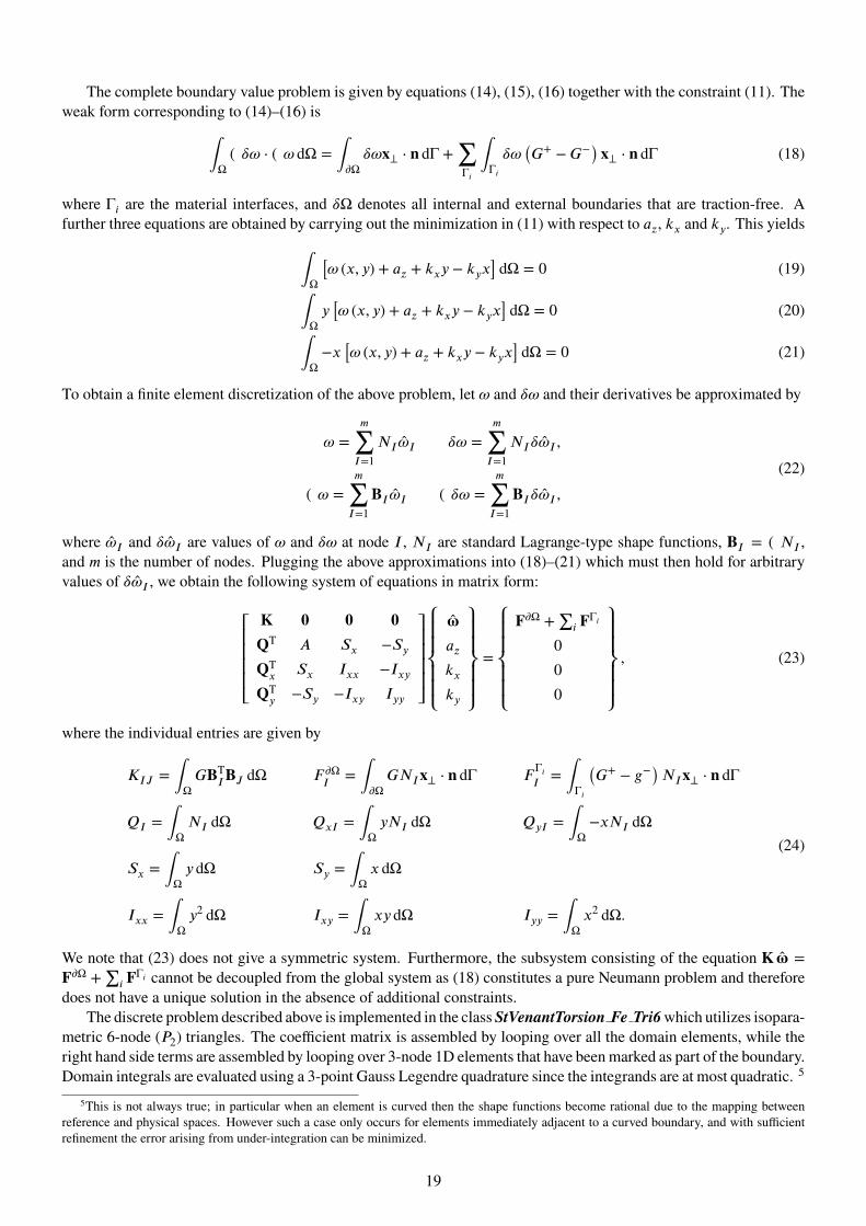
The complete boundary value problem is given by equations (14), (15), (16) together with the constraint (11). Theweak form corresponding to (14)–(16) is

ˆ

Ω∇�! ⋅ ∇! dΩ =

ˆ

)Ω�!x⟂ ⋅ n dΓ +

∑Γi

ˆ

Γi�!

(G+ − G−

)x⟂ ⋅ n dΓ (18)

where Γi are the material interfaces, and �Ω denotes all internal and external boundaries that are traction-free. Afurther three equations are obtained by carrying out the minimization in (11) with respect to az, kx and ky. This yields

ˆ

Ω

[! (x, y) + az + kxy − kyx

]dΩ = 0 (19)

ˆ

Ωy[! (x, y) + az + kxy − kyx

]dΩ = 0 (20)

ˆ

Ω−x

[! (x, y) + az + kxy − kyx

]dΩ = 0 (21)

To obtain a finite element discretization of the above problem, let ! and �! and their derivatives be approximated by

! =m∑I=1

NI !I �! =m∑I=1

NI�!I ,

∇! =m∑I=1BI !I ∇�! =

m∑I=1BI�!I ,

(22)

where !I and �!I are values of ! and �! at node I , NI are standard Lagrange-type shape functions, BI = ∇NI ,and m is the number of nodes. Plugging the above approximations into (18)–(21) which must then hold for arbitraryvalues of �!I , we obtain the following system of equations in matrix form:

⎡⎢⎢⎢⎢⎣

K 0 0 0QT A Sx −SyQTx Sx Ixx −IxyQTy −Sy −Ixy Iyy

⎤⎥⎥⎥⎥⎦

⎧⎪⎪⎨⎪⎪⎩

!azkxky

⎫⎪⎪⎬⎪⎪⎭

=

⎧⎪⎪⎨⎪⎪⎩

F)Ω +∑i FΓi

000

⎫⎪⎪⎬⎪⎪⎭

, (23)

where the individual entries are given by

KIJ =ˆ

ΩGBTIBJ dΩ F )ΩI =

ˆ

)ΩGNIx⟂ ⋅ n dΓ F ΓiI =

ˆ

Γi

(G+ − g−

)NIx⟂ ⋅ n dΓ

QI =ˆ

ΩNI dΩ QxI =

ˆ

ΩyNI dΩ QyI =

ˆ

Ω−xNI dΩ

Sx =ˆ

Ωy dΩ Sy =

ˆ

Ωx dΩ

Ixx =ˆ

Ωy2 dΩ Ixy =

ˆ

Ωxy dΩ Iyy =

ˆ

Ωx2 dΩ.

(24)

We note that (23) does not give a symmetric system. Furthermore, the subsystem consisting of the equation K! =F)Ω +

∑i FΓi cannot be decoupled from the global system as (18) constitutes a pure Neumann problem and therefore

does not have a unique solution in the absence of additional constraints.The discrete problem described above is implemented in the class StVenantTorsion Fe Tri6 which utilizes isopara-

metric 6-node (P2) triangles. The coefficient matrix is assembled by looping over all the domain elements, while theright hand side terms are assembled by looping over 3-node 1D elements that have been marked as part of the boundary.Domain integrals are evaluated using a 3-point Gauss Legendre quadrature since the integrands are at most quadratic. 5

5This is not always true; in particular when an element is curved then the shape functions become rational due to the mapping betweenreference and physical spaces. However such a case only occurs for elements immediately adjacent to a curved boundary, and with sufficientrefinement the error arising from under-integration can be minimized.

19

(a)

10−1 10010−7

10−6

10−5

10−4

10−3

10−2

cubic

ℎ

ë

Ω( !

exact−!ℎ) 2

dΩ

(b)

Figure 3: Saint-Venant torsion of a bar with elliptical cross section: (a) FE solution of the warping function ! usingisoparametric 6-node triangles, and (b) convergence of ! to the analytical solution with hierarchical refinement of themesh.

(a) (b)

Figure 4: Numerical results showing (a) the warping function!, and (b) the displacement component uz for an ellipticalcross-section centered at (1, 0.5).

Meanwhile, the boundary terms are calculated using a 3-point quadrature rule in 1D as explained in Appendix B. Froman implementation perspective, the system shown in (23) is interesting as the Dof objects corresponding to az, kx andky are not connected to any particular element. Instead they are associated with the Numerics instance itself, whichimplies that only one such object should be instantiated for the entire problem; inhomogeneity is handled through theuse of appropriate Material objects which provide the necessary shear modulus for each subdomain.

To verify the implementation, we examine the case of a shaft with an elliptical cross section centered at (0, 0) withmajor axis oriented along the x-direction. In this particular case the analytical solution for the warping function isgiven by[15]

! (x, y) = −a2 − b2a2 + b2

xy. (25)where a and b are the respective lengths of the semi-major and semi-minor axes. For the numerical simulation, wetake a = 2 and b = 1, and the shear modulus and rate of twist are also set to unity, i.e., G = � = 1. The finite elementsolution for ! (x, y) is plotted in Figure 3a for the coarsest mesh used in the study. Furthermore, we can see fromFigure 3b that the convergence rate with respect to mesh refinement is slightly better than cubic. This is to be expectedfor this particular case, i.e., even though the analytical solution is contained in the approximation space used, it isnonetheless impossible to reproduce it exactly as representation of the geometry with 6-node triangles results in theouter layer of elements having curved edges. Also, the warping function itself is physically meaningful only when thecenter of twist coincides with the origin. For cross sections having their center of twist elsewhere, the cross sectionalwarping is given by uz which must be calculated according to (10c). This is illustrated in Figure 4.

20

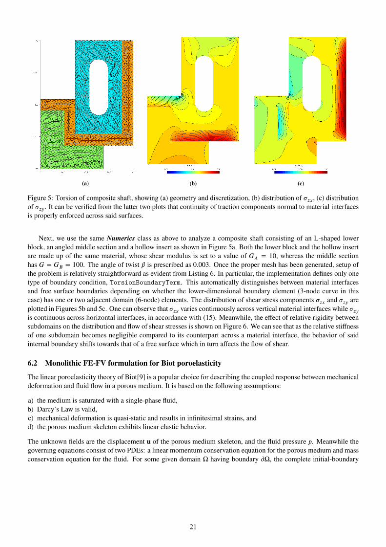
(a) (b) (c)

Figure 5: Torsion of composite shaft, showing (a) geometry and discretization, (b) distribution of �zx, (c) distributionof �zy. It can be verified from the latter two plots that continuity of traction components normal to material interfacesis properly enforced across said surfaces.

Next, we use the same Numerics class as above to analyze a composite shaft consisting of an L-shaped lowerblock, an angled middle section and a hollow insert as shown in Figure 5a. Both the lower block and the hollow insertare made up of the same material, whose shear modulus is set to a value of GA = 10, whereas the middle sectionhas G = GB = 100. The angle of twist � is prescribed as 0.003. Once the proper mesh has been generated, setup ofthe problem is relatively straightforward as evident from Listing 6. In particular, the implementation defines only onetype of boundary condition, TorsionBoundaryTerm. This automatically distinguishes between material interfacesand free surface boundaries depending on whether the lower-dimensional boundary element (3-node curve in thiscase) has one or two adjacent domain (6-node) elements. The distribution of shear stress components �zx and �zy areplotted in Figures 5b and 5c. One can observe that �zx varies continuously across vertical material interfaces while �zyis continuous across horizontal interfaces, in accordance with (15). Meanwhile, the effect of relative rigidity betweensubdomains on the distribution and flow of shear stresses is shown on Figure 6. We can see that as the relative stiffnessof one subdomain becomes negligible compared to its counterpart across a material interface, the behavior of saidinternal boundary shifts towards that of a free surface which in turn affects the flow of shear.

6.2 Monolithic FE-FV formulation for Biot poroelasticity

The linear poroelasticity theory of Biot[9] is a popular choice for describing the coupled response between mechanicaldeformation and fluid flow in a porous medium. It is based on the following assumptions:a) the medium is saturated with a single-phase fluid,b) Darcy’s Law is valid,c) mechanical deformation is quasi-static and results in infinitesimal strains, andd) the porous medium skeleton exhibits linear elastic behavior.The unknown fields are the displacement u of the porous medium skeleton, and the fluid pressure p. Meanwhile thegoverning equations consist of two PDEs: a linear momentum conservation equation for the porous medium and massconservation equation for the fluid. For some given domain Ω having boundary )Ω, the complete initial-boundary

21

Listing 6: Input file for torsion of composite shaft.1 *MESH_READER GmshReader2 *MESH_FILE CompositeSection.msh34 *SOLUTION_STAGES 15 *FIELDS_PER_NODE 26 *FIELDS_PER_CELL 478 *DOF_PER_NODE 19 1 DofGroup 1 NodalField 1 2

10 *DOF_PER_CELL 01112 *NUMERICS 113 1 StVenantTorsion_Fe_Tri614 NodalDof 115 Stage 116 Subsystem 117 CellFieldOutput 418 1 s_zx19 2 s_zy20 3 s_mag21 4 u_z22 TwistPerLength 0.00323 DofGroup 12425 *MATERIALS 226 1 LinearIsotropicElasticity Torsion 10027 2 LinearIsotropicElasticity Torsion 102829 *DOMAIN_ASSIGNMENTS 330 "LowerBlock" Numerics 1 MaterialSet 131 "InnerAngle" Numerics 1 MaterialSet 232 "HollowInsert" Numerics 1 MaterialSet 13334 *OUTPUT_FORMAT Gmsh35 FILENAME Torsion36 OUTPUT_STYLE ascii37 NODE_DATA 138 SCALAR WarpingFunction 139 ELEMENT_DATA 040 ELEMENT_NODE_DATA 541 SCALAR Stress_zx 142 SCALAR Stress_zy 243 SCALAR Stress_magnitude 344 VECTOR StressVector 1 2 045 SCALAR Z_Displacement 44647 *CSV_OUTPUT 04849 *LOADSTEPS 150 1 PREPROCESSING 051 START_TIME 0.052 END_TIME 1.053 INITIAL_TIME_INCREMENT 1.054 MAX_SUBSTEPS 10055 BOUNDARY_CONDITIONS 156 "LateralSurface" 1 TorsionBoundaryTerm 1 None57 FIELD_CONDITIONS 058 SOLUTION_METHODS59 Stage 1 LinearStatic60 LinearSolver MKL_Pardiso nThreads 12 Unsymmetric61 WRITE_INTERVAL 062 POSTPROCESSING 063 *END

22

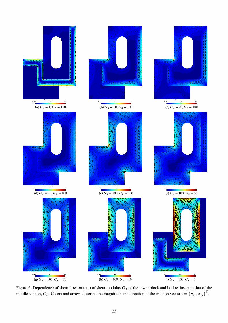
(a) GA = 1, GB = 100 (b) GA = 10, GB = 100 (c) GA = 20, GB = 100

(d) GA = 50, GB = 100 (e) GA = 100, GB = 100 (f) GA = 100, GB = 50

(g) GA = 100, GB = 20 (h) GA = 100, GB = 10 (i) GA = 100, GB = 1

Figure 6: Dependence of shear flow on ratio of shear modulus GA of the lower block and hollow insert to that of themiddle section, GB. Colors and arrows describe the magnitude and direction of the traction vector t = {

�zx, �zy}T.

23

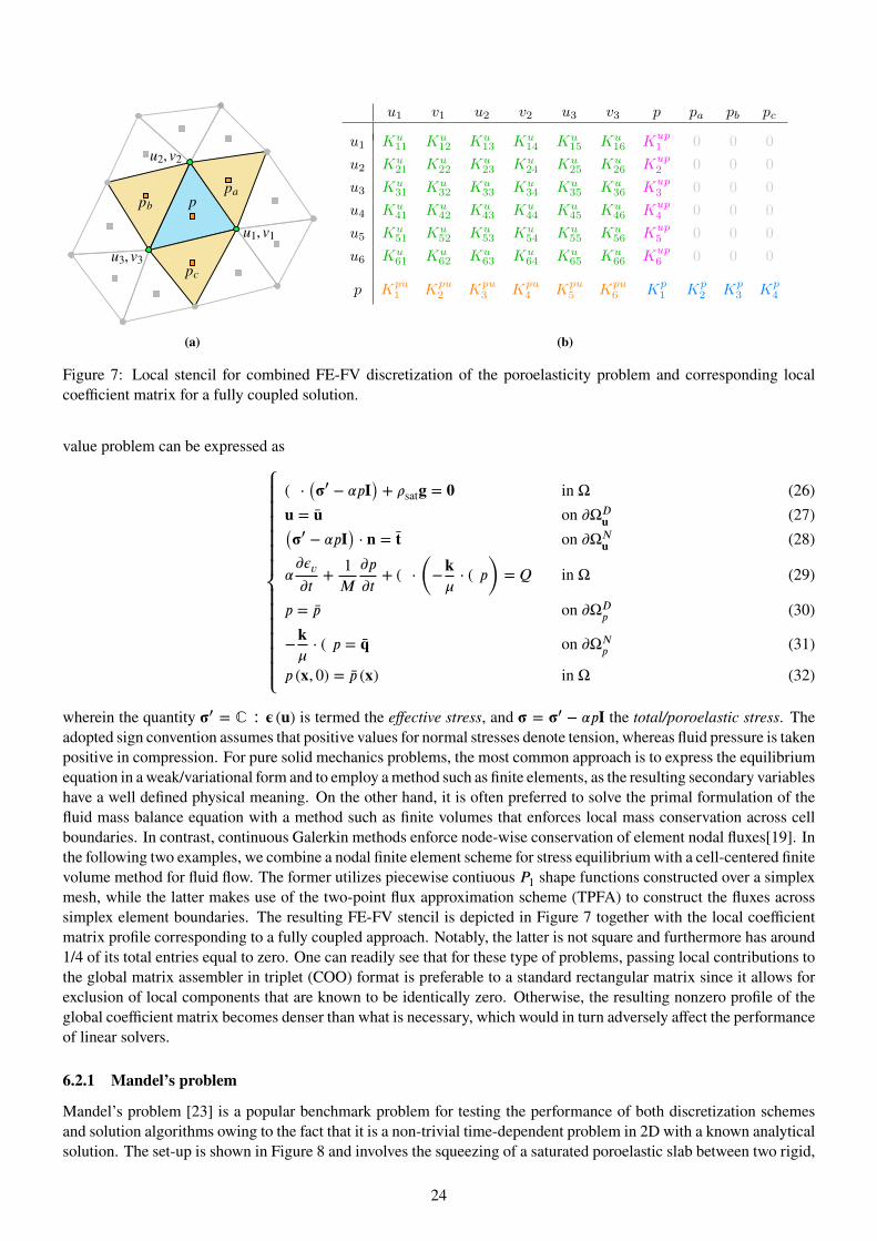
(a)

u1 v1 u2 v2 u3 v3 p pa pb pc

u1 Ku11 Ku

12 Ku13 Ku

14 Ku15 Ku

16 Kup1 0 0 0

u2 Ku21 Ku

22 Ku23 Ku

24 Ku25 Ku

26 Kup2 0 0 0

u3 Ku31 Ku

32 Ku33 Ku

34 Ku35 Ku

36 Kup3 0 0 0

u4 Ku41 Ku

42 Ku43 Ku

44 Ku45 Ku

46 Kup4 0 0 0

u5 Ku51 Ku

52 Ku53 Ku

54 Ku55 Ku

56 Kup5 0 0 0

u6 Ku61 Ku

62 Ku63 Ku

64 Ku65 Ku

66 Kup6 0 0 0

p Kpu1 Kpu

2 Kpu3 Kpu

4 Kpu5 Kpu

6 Kp1 Kp

2 Kp3 Kp

4

(b)

Figure 7: Local stencil for combined FE-FV discretization of the poroelasticity problem and corresponding localcoefficient matrix for a fully coupled solution.

value problem can be expressed as⎧⎪⎪⎪⎪⎪⎪⎨⎪⎪⎪⎪⎪⎪⎩

∇ ⋅(�′ − �pI

)+ �satg = 0 in Ω (26)

u = u on )ΩDu (27)(�′ − �pI

)⋅ n = t on )ΩNu (28)

�)�v)t

+ 1M)p)t+ ∇ ⋅

(−k�⋅ ∇p

)= Q in Ω (29)

p = p on )ΩDp (30)−k�⋅ ∇p = q on )ΩNp (31)

p (x, 0) = p (x) in Ω (32)

wherein the quantity �′ = ℂ ∶ � (u) is termed the effective stress, and � = �′ − �pI the total/poroelastic stress. Theadopted sign convention assumes that positive values for normal stresses denote tension, whereas fluid pressure is takenpositive in compression. For pure solid mechanics problems, the most common approach is to express the equilibriumequation in a weak/variational form and to employ a method such as finite elements, as the resulting secondary variableshave a well defined physical meaning. On the other hand, it is often preferred to solve the primal formulation of thefluid mass balance equation with a method such as finite volumes that enforces local mass conservation across cellboundaries. In contrast, continuous Galerkin methods enforce node-wise conservation of element nodal fluxes[19]. Inthe following two examples, we combine a nodal finite element scheme for stress equilibrium with a cell-centered finitevolume method for fluid flow. The former utilizes piecewise contiuous P1 shape functions constructed over a simplexmesh, while the latter makes use of the two-point flux approximation scheme (TPFA) to construct the fluxes acrosssimplex element boundaries. The resulting FE-FV stencil is depicted in Figure 7 together with the local coefficientmatrix profile corresponding to a fully coupled approach. Notably, the latter is not square and furthermore has around1/4 of its total entries equal to zero. One can readily see that for these type of problems, passing local contributions tothe global matrix assembler in triplet (COO) format is preferable to a standard rectangular matrix since it allows forexclusion of local components that are known to be identically zero. Otherwise, the resulting nonzero profile of theglobal coefficient matrix becomes denser than what is necessary, which would in turn adversely affect the performanceof linear solvers.

6.2.1 Mandel’s problem

Mandel’s problem [23] is a popular benchmark problem for testing the performance of both discretization schemesand solution algorithms owing to the fact that it is a non-trivial time-dependent problem in 2D with a known analyticalsolution. The set-up is shown in Figure 8 and involves the squeezing of a saturated poroelastic slab between two rigid,

24

2F

2F

2a

2b

(a)

F

a

b q · n = 0ux = 0

q · n = 0, uy = 0

q · n = 0, uy = uniform

h= 0t = 0

(b)

Figure 8: Setup for Mandel’s problem, showing (a) full geometry, and (b) computational domain.

frictionless and impervious plates. The slab and plates are assumed to extend infinitely along the out-of-plane (z)direction so that deformation follows plane strain conditions, i.e., uz = 0, and ux and uy are independent of z. Due tothe problem symmetry, it suffices to consider only the quarter domain (0, a) × (0, b), for which the relevant boundaryconditions are as follows:

ux = 0 on x = 0 (33a)uy = 0 on y = 0 (33b)uy = u (t) on y = b (33c)

ˆ a

0

(�′yy − p

)dx = −F on y = b (33d)

�xy = �xx = p = 0 on x = a (33e)(−k�⋅ ∇p

)⋅ n = 0 on x = 0, y = 0 and y = b. (33f)

In addition, initial conditions are set to zero for both u and p. Rigidity of the plates along with problem symmetryimplies a uniform vertical displacement u at y = b that is a priori unknown but dependent only on time. To achievethis condition, one must be able to constrain all degrees of freedom pertaining to uy on the top boundary to have thesame value. BROOMStyx allows the end user to specify master/slave types of constraints in the input file, by selectingone master DOF (e.g., the one residing on the node located at (0, b)) and declaring all other uy DOFs on y = b asslaves. The constraint is enforced in a strong sense during the simulation: unknowns associated with the slave DOFsare eliminated from the system of equations prior to determining the global sparse matrix structure. This also lumpsthe right hand side terms (i.e. resultant forces) onto the master DOF, which corresponds to the integral-type conditiongiven in (33d).

Analytical expressions for the displacements and stresses have been derived by Abousleiman et al.[2], supplement-ing the original solution of Mandel[23] for the pressure. Due to the instantaneous application of external loading, thesolutions are time-discontinuous at t = 0. Material properties for the current simulation are taken from the paper ofMikelic et al.[24] and are listed in Table 5. A comparison of analytical and numerical solutions is shown in Figure9. We can observe that the combined FE-FV scheme yields numerical results of the pressure that are in very goodagreement with the analytical solution.

6.2.2 Terzaghi 1-D consolidation

The consolidation of a layered porous medium under a uniform external distributed load was initially proposed in Hagaet al. [18], and later utilized by Rodrigo et al. [30] to demonstrate the occurrence of numerical oscillations in finiteelement solutions for the pressure at early times even when inf-sup stable elements are used. The problem domain is asquare having each side of unit measure and consisting of a middle region of low permeability sandwiched between two

25

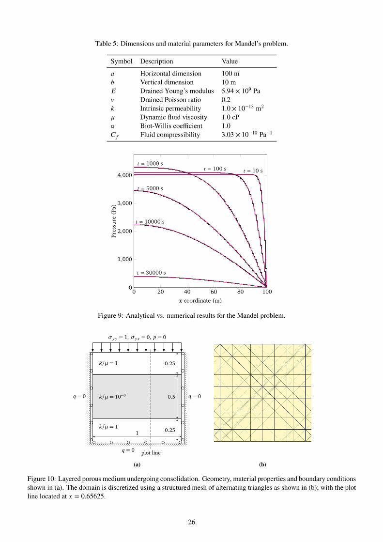
Table 5: Dimensions and material parameters for Mandel’s problem.

Symbol Description Valuea Horizontal dimension 100 mb Vertical dimension 10 mE Drained Young’s modulus 5.94 × 109 Pa� Drained Poisson ratio 0.2k Intrinsic permeability 1.0 × 10−13 m2

� Dynamic fluid viscosity 1.0 cP� Biot-Willis coefficient 1.0Cf Fluid compressibility 3.03 × 10−10 Pa−1

0 20 40 60 80 1000

1,000

2,000

3,000

4,000t = 10 st = 100 s

t = 1000 s

t = 5000 s

t = 10000 s

t = 30000 s

x-coordinate (m)

Pressure

(Pa)

Figure 9: Analytical vs. numerical results for the Mandel problem.

σy y = 1, σy x = 0, p = 0

1 0.25

0.5

0.25

k/µ= 1

k/µ= 10−8

k/µ= 1

q = 0

q = 0q = 0

plot line

(a) (b)

Figure 10: Layered porous medium undergoing consolidation. Geometry, material properties and boundary conditionsshown in (a). The domain is discretized using a structured mesh of alternating triangles as shown in (b); with the plotline located at x = 0.65625.

26

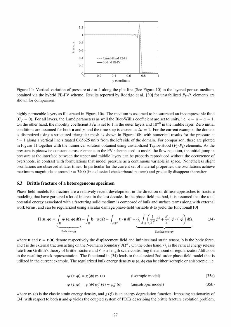
0 0.2 0.4 0.6 0.8 10

0.2

0.4

0.6

0.8

1

1.2

y-coordinate

Pressure

Unstabilized P2-P1Hybrid FE-FV

Figure 11: Vertical variation of pressure at t = 1 along the plot line (See Figure 10) in the layered porous medium,obtained via the hybrid FE-FV scheme. Results reported by Rodrigo et al. [30] for unstabilized P2-P1 elements areshown for comparison.

highly permeable layers as illustrated in Figure 10a. The medium is assumed to be saturated an incompressible fluid(Cf = 0). For all layers, the Lame parameters as well the Biot-Willis coefficient are set to unity, i.e. � = � = � = 1.On the other hand, the mobility coefficient k∕� is set to 1 in the outer layers and 10−8 in the middle layer. Zero initialconditions are assumed for both u and p, and the time step is chosen as Δt = 1. For the current example, the domainis discretized using a structured triangular mesh as shown in Figure 10b, with numerical results for the pressure att = 1 along a vertical line situated 0.65625 units from the left side of the domain. For comparison, these are plottedin Figure 11 together with the numerical solution obtained using unstabilized Taylor-Hood (P2-P1) elements. As thepressure is piecewise constant across elements in the FV scheme used to model the flow equation, the initial jump inpressure at the interface between the upper and middle layers can be properly reproduced without the occurrence ofovershoots, in contrast with formulations that model pressure as a continuous variable in space. Nonetheless slightoscillations are observed at later times. In particular for the current set of material properties, the oscillations achievemaximum magnitude at around t = 3400 (in a classical checkerboard pattern) and gradually disappear thereafter.

6.3 Brittle fracture of a heterogeneous specimen

Phase-field models for fracture are a relatively recent development in the direction of diffuse approaches to fracturemodeling that have garnered a lot of interest in the last decade. In the phase-field method, it is assumed that the totalpotential energy associated with a fracturing solid medium is composed of bulk and surface terms along with externalwork terms, and can be regularized using a scalar damage/phase-field variable � to yield the functional[10]

Π (u, �) =ˆ

Ω (�, �) dΩ

⏟⏞⏞⏞⏞⏞⏞⏟⏞⏞⏞⏞⏞⏞⏟Bulk energy

−ˆ

Ωb ⋅ u dΩ −

ˆ

)ΩNt ⋅ u dΓ + c

ˆ

Ω

(12l�2 + l

2∇� ⋅ ∇�

)dΩ

⏟⏞⏞⏞⏞⏞⏞⏞⏞⏞⏞⏞⏞⏞⏞⏞⏞⏞⏞⏞⏞⏞⏞⏟⏞⏞⏞⏞⏞⏞⏞⏞⏞⏞⏞⏞⏞⏞⏞⏞⏞⏞⏞⏞⏞⏞⏟Surface energy

, (34)

where u and � = � (u) denote respectively the displacement field and infinitesimal strain tensor, b is the body force,and t is the external traction acting on the Neumann boundary )ΩN . On the other hand, c is the critical energy releaserate from Griffith’s theory of brittle fracture and l is a length scale controlling the amount of regularization/diffusionin the resulting crack representation. The functional in (34) leads to the classical 2nd-order phase-field model that isutilized in the current example. The regularized bulk energy density (�, �) can be either isotropic or anisotropic, i.e.

(�, �) = g (�) 0 (�) (isotropic model) (35a) (�, �) = g (�) +0 (�) +

−0 (�) (anisotropic model) (35b)

where 0 (�) is the elastic strain energy density, and g (�) is an energy degradation function. Imposing stationarity of(34) with respect to both u and � yields the coupled system of PDEs describing the brittle fracture evolution problem,

27

expressed in weak form as⎧⎪⎪⎨⎪⎪⎩

ˆ

Ω

) )�

∶ �� dΩ =ˆ

Ωu ⋅ �� dΩ +

ˆ

)ΩNt ⋅ �u dΓ (36)

ˆ

Ω

) )��� d٠+

ˆ

Ωc

(l∇� ⋅ ∇�� + 1

l� ��

)dΩ = 0 (37)

Owing to the form of (�, �), the above system represents a nonlinear set of equations that must be solved via anapproach that can handle the non-convexity of (34). In BROOMStyx, (36)–(37) is implemented via the class Phase-FieldFracture Fe Tri3 which assumes 2D plane strain conditions. Furthermore, (�, �) is implemented as a Materialclass through a composition strategy, in that it contains among its members additional material objects correspondingto elasticity models and degradation functions. This maximizes code reuse, since several different models for (�, �)have been proposed in the literature. Here we make use of the anisotropic model of Amor et al.[4] that enforces theunilateral contact condition through a volumetric/deviatoric splitting of the energy. Let � = {

�xx, �yy, 0, xy}T be the

symmetric strain tensor in Voigt form. 6 Its volumetric and deviatoric components can then be calculated as�vol = ℙ� �dev = (I − ℙ) � (39)

wherein

I =⎡⎢⎢⎢⎣

1 0 0 00 1 0 00 0 1 00 0 0 1

⎤⎥⎥⎥⎦

and ℙ = 12

⎡⎢⎢⎢⎣

1 1 0 01 1 0 00 0 0 00 0 0 0

⎤⎥⎥⎥⎦, (40)

with the given form of ℙ being specific for 2D analysis. 7 Then for some strain energy function 0 (�), we obtain 0,vol (�) = 0

(�vol

) 0,dev (�) = 0

(�dev

) (41)Likewise, the stress decomposition is given by

�vol =d 0

(�vol

)d�

�dev =d 0

(�dev

)d�

(42)On the other hand, the derivatives of �vol and �dev with respect to the strain are

ℂvol =d�vold�

=d2 0

(�vol

)d� d�

ℙ ℂdev =d�devd�

=d2 0

(�dev

)d� d�

(I − ℙ) , (43)both of which are asymmetric. Nevertheless, the products BTℂvolB and BTℂdevB yield symmetric matrices due to theparticular form of B in plane strain (see footnote 6). In Amor et al.[4], the damage-degraded bulk energy density isgiven as

(�, �) = g (�)[ 0

(�+vol

)+ 0

(�dev

)]+ 0

(�−vol

), (44)

wherein �+vol = H (tr �) �vol and �−vol = H (− tr �) �vol with H (∙) denoting the Heaviside step function. This is imple-mented in the material class AmorDamageModel, which as previously mentioned requires also the specification offurther classes to calculate quantities related to the basic elasticity model as well as the energy degradation function,for instance as illustrated in Table 6. The parent material model makes the appropriate calls to its child objects to

6It is assumed that constitutive models return the elasticity tensor as a 3 × 3 matrix when in plane stress mode, 4 × 4 in plane strain andaxisymmetric analysis, and 6 × 6 for the full 3D case; the use of a rank-4 matrix in plane strain is due to the fact that the stress component �zzis needed when dealing with plasticity. However since �zz = 0 in plane strain, the symmetrized gradient matrix B that is used to obtain strainsfrom displacements via the operation � = Bu has hard-coded zeros corresponding to the row for �zz, i.e.

B =

⎡⎢⎢⎢⎢⎣

N1,x 0 N2,x 0 …0 N1,y 0 N2,y …0 0 0 0 …N1,y N1,x N2,y N2,x …

⎤⎥⎥⎥⎥⎦

(38)

7The decomposition of � into volumetric and deviatoric components is normally written as � = 1n�vI+�dev, in which �v = tr (�) and n = 3, so

that tr (�dev)= 0. However in plane strain, �zz is identically zero hence �v = �xx + �yy. For the current problem, we perform the decomposition

assuming n = 2, such that in the 3rd dimension �zz,vol = �zz,dev = 0. This of course means that �vol is no longer isotropic in a full 3D context.

28

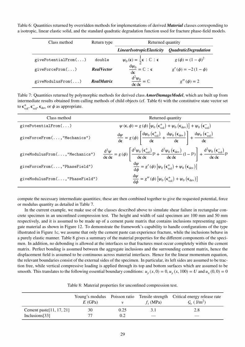
Table 6: Quantities returned by overridden methods for implementations of derived Material classes corresponding toa isotropic, linear elastic solid, and the standard quadratic degradation function used for fracture phase-field models.

Class method Return type Returned quantityLinearIsotropicElasticity QuadraticDegradation

givePotentialFrom(...) double 0 (�) =12� ∶ ℂ ∶ � g (�) = (1 − �)2

giveForceFrom(...) RealVectord 0d�

= ℂ ∶ � g′ (�) = −2 (1 − �)

giveModulusFrom(...) RealMatrixd2 0d� d�

= ℂ g′′ (�) = 2

Table 7: Quantities returned by polymorphic methods for derived class AmorDamageModel, which are built up fromintermediate results obtained from calling methods of child objects (cf. Table 6) with the constitutive state vector setto �+vol, �−vol, �dev or � as appropriate.

Class method Returned quantitygivePotentialFrom(...) (�, �) = g (�)

[ 0

(�+vol

)+ 0

(�dev

)]+ 0

(�−vol

)

giveForceFrom(...,"Mechanics")d d�

= g (�)

[d 0

(�+vol

)d�

+d 0

(�dev

)d�

]+d 0

(�−vol

)d�

giveModulusFrom(...,"Mechanics")d2 d� d�

= g (�)

[d2 0

(�+vol

)d� d�

ℙ +d2 0

(�dev

)d� d�

(I − ℙ)

]+d2 0

(�−vol

)d� d�

ℙ

giveForceFrom(...,"PhaseField")d d�

= g′ (�)[ 0

(�+vol

)+ 0

(�dev

)]

giveModulusFrom(...,"PhaseField")d d�

= g′′ (�)[ 0

(�+vol

)+ 0

(�dev

)]

compute the necessary intermediate quantities; these are then combined together to give the requested potential, forceor modulus quantity as detailed in Table 7.

In the current example, we make use of the classes described above to simulate shear failure in rectangular con-crete specimen in an unconfined compression test. The height and width of said specimen are 100 mm and 50 mmrespectively, and it is assumed to be made up of a cement paste matrix that contains inclusions representing aggre-gate material as shown in Figure 12. To demonstrate the framework’s capability to handle configurations of the typeillustrated in Figure 1c, we assume that only the cement paste can experience fracture, while the inclusions behave ina purely elastic manner. Table 8 gives a summary of the material properties for the different components of the speci-men. In addition, no debonding is allowed at the interfaces so that fractures must occur completely within the cementmatrix. Perfect bonding is assumed between the aggregate inclusions and the surrounding cement matrix, hence thedisplacement field is assumed to be continuous across material interfaces. Hence for the linear momentum equation,the relevant boundaries consist of the external sides of the specimen. In particular, its left sides are assumed to be trac-tion free, while vertical compressive loading is applied through its top and bottom surfaces which are assumed to besmooth. This translates to the following essential boundary conditions: uy (x, 0) = 0, uy (x, 100) = U and ux (0, 0) = 0

Table 8: Material properties for unconfined compression test.

Young’s modulus Poisson ratio Tensile strength Critical energy release rateE (GPa) � ft (MPa) c ( J/m2)

Cement paste[11, 17, 21] 30 0.25 3.1 2.8Inclusions[33] 77 0.2 — —

29

Figure 12: Concrete specimen in unconfined compression test, consisting of aggregate material (blue) embedded in acement paste matrix (gray).

with the last condition needed to ensure uniqueness of solutions. The final prescribed displacement at the top surfaceof the specimen is set to U = −0.0125 mm, which is applied incrementally, initially with Δuy = 5 × 10−4 mm andrefined to Δuy = 1 × 10−4 near the instance of failure. On the other hand for the phase-field equation, the relevantboundaries consist of the external surfaces of the specimen together with the interfaces between cement matrix andinclusions. The condition ∇� ⋅n = 0 is imposed on the external surfaces of the specimen, while at material interfaces,it is possible to impose either ∇� ⋅ n = 0 or � = 0. We use the standard quadratic degradation function

g (�) = (1 − �)2 , (45)and following Nguyen et al.[26] the value of the phase-field regularization parameter is calculated as

l =27Ec256f 2t

. (46)

Plugging in the values from Table 8 then yields l = 0.922 mm. As crack paths are a priori unknown, the problemdomain is discretized uniformly into triangular elements, with the characteristic size of element edges set to 0.23 mm.The resulting unstructured mesh contains a total of 112,806 nodes and 224,304 elements. In the matrix region, eachnode has three active degrees of freedom corresponding to ux, uy and �. On the other hand in regions corresponding toinclusions, only the displacement DOFs are active. Consequently the total number of active DOFs is between 293,000and 298,000 depending on the specific type of boundary conditions used for the phase-field equation.

We conduct two simulation runs to look at what effect the type of phase-field BC imposed at material interfaceshas on the predicted behavior of the specimen. As inclusions do not fracture, they are modeled using the numericsclass PlaneStrain Fe Tri3, which implements the stress equilibrium equation in 2D assuming plane strain conditions.The latter is “compatible” with the earlier described numerics class for phase-field fracture with respect to the stressequilibrium implementation, hence they can share the same set of displacement DOFs. However as these two classesare each assumed to have been coded without knowledge of one another, the task of setting up the simulation allowingfor their simultaneous use falls to the end user, who must globally declare the number of DOF types to be used andsubsequently assign them within the two classes in question so as to be recognized by the latter. This is done purelywithin the input file as illustrated in Listing 7, with no additional coding required. Likewise, subsystem numbers areassigned for each set of governing equations implemented in the numerics classes. This is necessary so that the rightsets of equations are grouped together in the subsequent solution steps. To solve the system of nonlinear equationsat each time step, we utilize a solution algorithm implemented in the class AlternateNonlinearMinimization, whichperforms a nested cycle of iterations to solve the coupled system of equations: the outer loop alternates between the

30

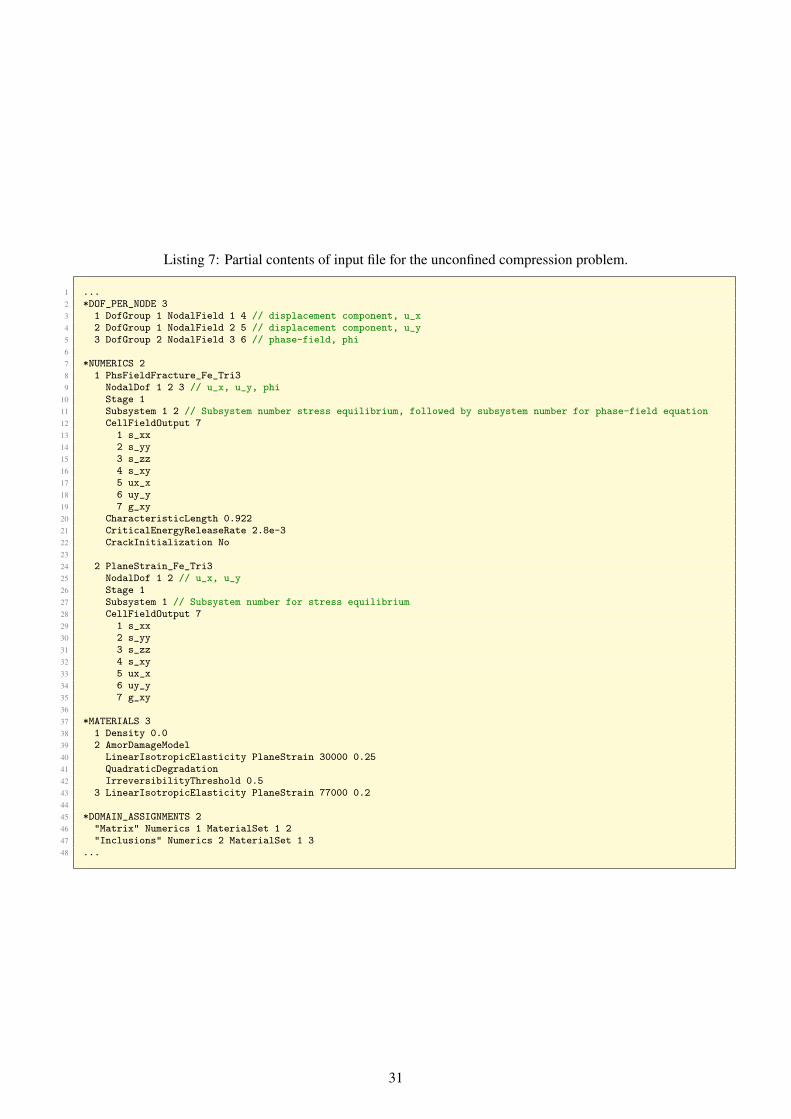
Listing 7: Partial contents of input file for the unconfined compression problem.1 ...2 *DOF_PER_NODE 33 1 DofGroup 1 NodalField 1 4 // displacement component, u_x4 2 DofGroup 1 NodalField 2 5 // displacement component, u_y5 3 DofGroup 2 NodalField 3 6 // phase-field, phi67 *NUMERICS 28 1 PhsFieldFracture_Fe_Tri39 NodalDof 1 2 3 // u_x, u_y, phi

10 Stage 111 Subsystem 1 2 // Subsystem number stress equilibrium, followed by subsystem number for phase-field equation12 CellFieldOutput 713 1 s_xx14 2 s_yy15 3 s_zz16 4 s_xy17 5 ux_x18 6 uy_y19 7 g_xy20 CharacteristicLength 0.92221 CriticalEnergyReleaseRate 2.8e-322 CrackInitialization No2324 2 PlaneStrain_Fe_Tri325 NodalDof 1 2 // u_x, u_y26 Stage 127 Subsystem 1 // Subsystem number for stress equilibrium28 CellFieldOutput 729 1 s_xx30 2 s_yy31 3 s_zz32 4 s_xy33 5 ux_x34 6 uy_y35 7 g_xy3637 *MATERIALS 338 1 Density 0.039 2 AmorDamageModel40 LinearIsotropicElasticity PlaneStrain 30000 0.2541 QuadraticDegradation42 IrreversibilityThreshold 0.543 3 LinearIsotropicElasticity PlaneStrain 77000 0.24445 *DOMAIN_ASSIGNMENTS 246 "Matrix" Numerics 1 MaterialSet 1 247 "Inclusions" Numerics 2 MaterialSet 1 348 ...

31

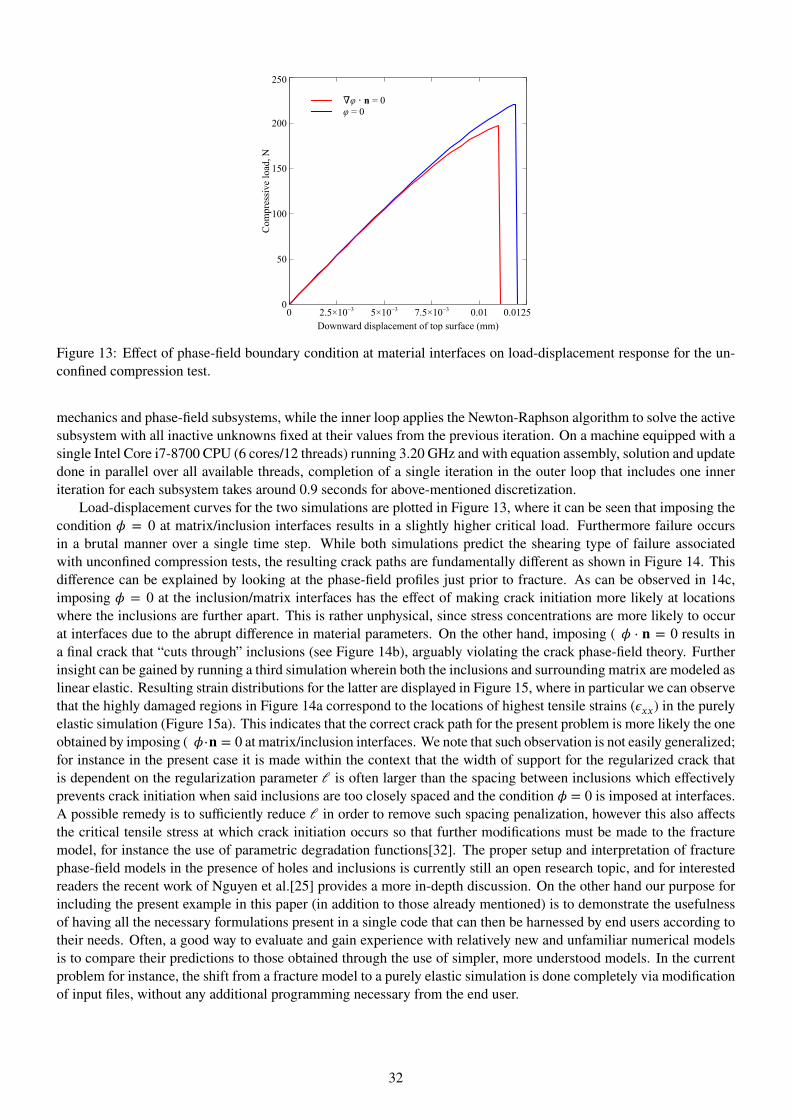
∇φ ⋅ n = 0φ = 0

Com

pres

sive

load

, N

0

50

100

150

200

250

Downward displacement of top surface (mm)0 2.5×10−3 5×10−3 7.5×10−3 0.01 0.0125

Figure 13: Effect of phase-field boundary condition at material interfaces on load-displacement response for the un-confined compression test.

mechanics and phase-field subsystems, while the inner loop applies the Newton-Raphson algorithm to solve the activesubsystem with all inactive unknowns fixed at their values from the previous iteration. On a machine equipped with asingle Intel Core i7-8700 CPU (6 cores/12 threads) running 3.20 GHz and with equation assembly, solution and updatedone in parallel over all available threads, completion of a single iteration in the outer loop that includes one inneriteration for each subsystem takes around 0.9 seconds for above-mentioned discretization.

Load-displacement curves for the two simulations are plotted in Figure 13, where it can be seen that imposing thecondition � = 0 at matrix/inclusion interfaces results in a slightly higher critical load. Furthermore failure occursin a brutal manner over a single time step. While both simulations predict the shearing type of failure associatedwith unconfined compression tests, the resulting crack paths are fundamentally different as shown in Figure 14. Thisdifference can be explained by looking at the phase-field profiles just prior to fracture. As can be observed in 14c,imposing � = 0 at the inclusion/matrix interfaces has the effect of making crack initiation more likely at locationswhere the inclusions are further apart. This is rather unphysical, since stress concentrations are more likely to occurat interfaces due to the abrupt difference in material parameters. On the other hand, imposing ∇� ⋅ n = 0 results ina final crack that “cuts through” inclusions (see Figure 14b), arguably violating the crack phase-field theory. Furtherinsight can be gained by running a third simulation wherein both the inclusions and surrounding matrix are modeled aslinear elastic. Resulting strain distributions for the latter are displayed in Figure 15, where in particular we can observethat the highly damaged regions in Figure 14a correspond to the locations of highest tensile strains (�xx) in the purelyelastic simulation (Figure 15a). This indicates that the correct crack path for the present problem is more likely the oneobtained by imposing∇�⋅n = 0 at matrix/inclusion interfaces. We note that such observation is not easily generalized;for instance in the present case it is made within the context that the width of support for the regularized crack thatis dependent on the regularization parameter l is often larger than the spacing between inclusions which effectivelyprevents crack initiation when said inclusions are too closely spaced and the condition � = 0 is imposed at interfaces.A possible remedy is to sufficiently reduce l in order to remove such spacing penalization, however this also affectsthe critical tensile stress at which crack initiation occurs so that further modifications must be made to the fracturemodel, for instance the use of parametric degradation functions[32]. The proper setup and interpretation of fracturephase-field models in the presence of holes and inclusions is currently still an open research topic, and for interestedreaders the recent work of Nguyen et al.[25] provides a more in-depth discussion. On the other hand our purpose forincluding the present example in this paper (in addition to those already mentioned) is to demonstrate the usefulnessof having all the necessary formulations present in a single code that can then be harnessed by end users according totheir needs. Often, a good way to evaluate and gain experience with relatively new and unfamiliar numerical modelsis to compare their predictions to those obtained through the use of simpler, more understood models. In the currentproblem for instance, the shift from a fracture model to a purely elastic simulation is done completely via modificationof input files, without any additional programming necessary from the end user.

32

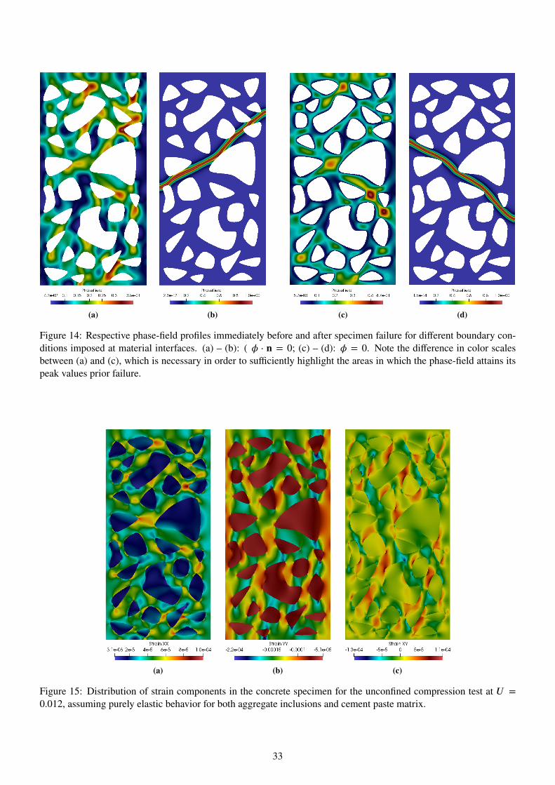
(a) (b) (c) (d)

Figure 14: Respective phase-field profiles immediately before and after specimen failure for different boundary con-ditions imposed at material interfaces. (a) – (b): ∇� ⋅ n = 0; (c) – (d): � = 0. Note the difference in color scalesbetween (a) and (c), which is necessary in order to sufficiently highlight the areas in which the phase-field attains itspeak values prior failure.

(a) (b) (c)

Figure 15: Distribution of strain components in the concrete specimen for the unconfined compression test at U =0.012, assuming purely elastic behavior for both aggregate inclusions and cement paste matrix.

33

7 Concluding remarks

In this paper, the design of BROOMStyx, an efficient object-oriented, multi-method and multiphysics frameworkhas been presented. The code architecture incorporates elements of both framework and library approaches in orderdeliver equal benefit to both model developers and end users. An important focus of the code is on maximizingflexibility available to end users through input file definitions, which has been demonstrated with several numericalexamples. Furthermore, BROOMStyx implements its own vector and matrix classes along with operator overloadingand a lazy evaluation strategy in order to improve code readability without sacrificing efficiency of execution. In orderto fully exploit the capabilities of machines having multiple-core processors, the code makes use of shared memoryparallelization via OpenMP directives.

At present, the BROOMStyx framework contains over 25,000 lines of code and serves as the main simulation toolused by the Author for computational research. Robustness of the code for handling different types of problems hasbeen demonstrated in the current work via several numerical examples. In particular we have shown that the code canaccommodate models featuring unknowns that are not associated with geometric entities, constraints involving masterand slave DOFs as well as the combination of fundamentally different numerical formulations within a monolithicsolution scheme. In addition, the framework can handle complicated nonlinear problems that require special solutionalgorithms. While current implemented models have so far been confined to 2D, the framework readily admits 3Dformulations without any modification to the core structure. Extension of the software to allow for distributed memoryparallelization through MPI routines is currently a work in progress, along with adaptive remeshing capabilities throughthe integration of existing libraries. It is hoped that the framework can serve as a platform upon which researcherscan implement new models and algorithms in a manner that can be immediately useful to engineers dealing with realworld problems, thus eventually speeding up the adoption of such innovations into mainstream industry. To this end,BROOMStyx is made available as open-source software under Version 3 of the GNU General Public License (GPLv3),and the source code can be downloaded from https://github.com/broomstyx/broomstyx.git.

Acknowledgements

This work was funded by the Research Council of Norway through grant no. 228832/E20 and Equinor ASA throughthe Akademia agreement. I am immensely grateful to Eirik Keilegavlen, Inga Berre and Jan M. Nordbotten for takingthe time to review the current manuscript and for their many suggestions that have helped to improve its content. Iwould also like to thank Robert Klofkorn for his many insights on advanced C++ programming that have aided megreatly in improving the overall structure of the BROOMStyx code.

A Alternate solution of torsion problem involving symmetric systems

The set of equations given in (23) are asymmetric, however they can be split into two consecutive solutions of sym-metric systems. As mentioned in the main discussion, the matrix equation K! = F)Ω +

∑i FΓi corresponds to a

pure Neumann problem so that the coefficient matrix K is rank-deficient by 1 and ! can be determined uniquely upto a constant. In such cases it is often the practice to artificially constrain one degree of freedom from the set {!I

},however a more elegant way is to introduce a Lagrange multiplier � for the purpose of imposing the constraint

ˆ

Ω!dΩ = 0. (47)

This results in the symmetric augmented system[K QQT 0

]{!�

}={F)Ω +

∑i FΓi

0

}, (48)

which now yields unique values for ! and �. The constants az, kx and ky can subsequently be determined by solvingthe system

⎡⎢⎢⎢⎣

A Sx −SySx Ixx −Ixy−Sy −Ixy Iyy

⎤⎥⎥⎥⎦

⎧⎪⎨⎪⎩

azkxky

⎫⎪⎬⎪⎭=⎧⎪⎨⎪⎩

0−QTx!−QTy !

⎫⎪⎬⎪⎭. (49)

34

While this method does not necessarily yield the same solution of ! as (23), they lead to the same expression foruz (x, y), which is after all the relevant quantity describing the cross sectional warping for an arbitrary cross section.

B Evaluation of boundary terms on curved edges

In Section 6.1, a right hand side term must be evaluated for elements having edges that coincide with interior or exteriorboundaries of the bar cross section, given by

F eI =ˆ

)ΩeNeIx⟂ ⋅ n dΓ (50)

As the chosen FE discretization makes use of 6-node isoparametric elements, the element edges over which the aboveterm is calculated (and which in general may be curved) can be treated as 3-node isoparametric 1D elements. For thelatter, we assume that a curved element in 2D Cartesian space maps to a master element having nodes at referencecoordinates � = −1, � = 0 and � = 1. The spatial coordinates are given by

x (�) =3∑I=1

NeI (�) xI =

{x (�)y (�)

}(51)

where NI are the Lagrange shape functions corresponding to a 2nd degree polynomial. On the other hand, n is givenby

n (�) = b√x′ (�) ⋅ x′ (�)

{−y′ (�)x′ (�)

}(52)

in which b has a value of either +1 or −1 such that n points outward from the associated domain element. Finally, dΓis given by

dΓ =√dx ⋅ dx =

√x′ (�) ⋅ x′ (�)d� (53)

Making use of the above expressions and noting that x⟂ (�) = {−y (�) , x (�)}T, we can rewrite (50) as

F eI =ˆ 1

−1bNe

I (�)[y (�) y′ (�) + x (�) x′ (�)

]d� (54)

As NI is of degree 2, the expression above involves integration of a 5th degree polynomial. In the code, a 3-pointGauss quadrature is used to obtain exact results.

References

[1] Intel® math kernel library for linux*. https://software.intel.com/en-us/mkl, 2019.[2] Y. Abousleiman, A. H.-D. Cheng, L. Cui, E. Detournay, and J.-C. Roegiers. Mandel’s problem revisited.

Geotechnique, 42(2):187–195, 1996.[3] Martin S. Alnæs, Anders Logg, Kristian B. Ølgaard, Marie E. Rognes, and Garth N. Wells. Unified form lan-

guage: A domain-specific language for weak formulations of partial differential equations. ACM Trans. Math.Softw., 40(2):9:1–9:37, 2014.

[4] H. Amor, J.-J. Marigo, and C. Maurini. Regularized formulation of the variational brittle fracture with unilateralcontact: Numerical experiments. J. Mech. Phys. Solids, 57:1209–1229, 2009.

[5] Utkarsh Ayachit. The ParaView Guide: A Parallel Visualization Application. Kitware, Inc., USA, 2015.[6] W. Bangerth, R. Hartmann, and G. Kanschat. deal.II – a General Purpose Object Oriented Finite Element Library.

ACM Trans. Math. Softw., 33(4):24/1–24/27, 2007.[7] P. Bastian, M. Droske, Engwer C., R. Klofkorn, T. Neubauer, M. Ohlberger, and M. Rumpf. Towards a unified

framework for scientific computing. In Proceedings of the 15th International Conference on Domain Decom-position Methods, Berlin, 2003. Proceedings of the 15th International Conference on Domain DecompositionMethods.

35

[8] T. Belytschko, Y. Y. Lu, and L. Gu. Element-free galerkin methods. Int. J. Numer. Meth. Engrg., 37:229–256,1994.

[9] M.A. Biot. General theory of three-dimensional consolidation. J. Appl. Phys., 12(2):155–164, 1941.[10] B. Bourdin, G. A. Francfort, and J.-J. Marigo. The variational approach to fracture. J. Elasticity, 91:5–148, 2008.[11] J. H. Brown and C. D. Pomeroy. Fracture toughness of cement paste and mortars. Cem. Concr. Res., 3:475–480,

1973.[12] R. W. Clough. Early history of the finite element method from the view point of a pioneer. Int. J. Numer. Meth.

Engng., 60:283–287, 2004.[13] Dassault Systemes. Abaqus 2016 online documentation. http://abaqus.software.polimi.it/v2016/, 2016.[14] A. Dedner, R. Klofkorn, M. Nolte, and M. Ohlberger. A generic interface for parallel and adaptive discretization

schemes: abstraction principles and the Dune-Fem module. Computing, 90(3):165–196, 2010.[15] Y. C. Fung. Foundations of Solid Mechanics. Prentice Hall, New Jersey, 1965.[16] C. Geuzaine and J.-F. Remacle. Gmsh: A 3-d finite element mesh generator with built-in pre- and post-processing

facilities. Int. J. Numer. Meth. Engng., 79:1309–1331, 2009.[17] C.-J. Haecker, E. J. Garboczi, J. W. Bullard, R. B. Bohn, Z. Sun, S. P. Shah, and T. Voigt. Modeling the linear

elastic properties of portland cement paste. Cem. Concr. Res., 35:1948–1960, 2005.[18] J. B. Haga, H. Osnes, and H. P. Langtangen. On the causes of pressure oscillations in low-permeable and low-

compressible porous media. Int. J. Numer. Anal. Meth. Geomech., 36:1507–1522, 2012.[19] T. J. R. Hughes, G. Engel, L. Mazzei, and M. G. Larson. The continuous galerkin method is locally conservative.

J. Comput. Phys., 163:467–488, 2000.[20] M. Lehn, A. Stippler, and K. Urban. Flens – a flexible library for efficient numerical solutions. In Proceedings

of Equadiff 11, Proceedings of minisymposia and contributed talks, pages 467–473. Proceedings of Equadiff 11,Proceedings of minisymposia and contributed talks, Comenius University Press, July 25–29 2005.

[21] Y. Li and J. Li. Relationship between fracture area and tensile strength of cement paste with supplementarycementitious materials. Constr. Build. Mater., 79:223–228, 2015.

[22] A. Logg, K.-A. Mardal, and G.N. Wells, editors. Automated Solution of Differential Equations by the FiniteElement Method. Springer, 2012.

[23] J. Mandel. Consolidation des sols (etude mathematique). Geotechnique, 3(7):287–299, 1953.[24] A. Mikelic, B. Wang, and M. F. Wheeler. Numerical convergence study of iterative coupling for coupled flow

and geomechanics. Comput. Geosci., 18:325–341, 2014.[25] N. Nguyen, J. Yvonnet, J. Rethore, and A. B. Tran. Identification of fracture models based on phase field for

crack propagation in heterogeneous lattices in a context of non-separated scales. Comput. Mech., 2018.[26] T. Nguyen, J. Yvonnet, M. Bornert, C. Chateau, K. Sab, R. Romani, and R. Le Roy. On the choice of parameters

in the phase field method for simulating crack initiation with experimental validation. Int. J. Fract., 197:213–226,2016.

[27] B. Patzak and Z. Bittnar. Design of object oriented finite element code. Adv. Eng. Softw., 2:759–767, 2001.[28] J. R. Rice. A Path Independent Integral and the Approximate Analysis of Strain Concentration by Notches and

Cracks. J. Appl. Mech., 35:379–386, 1968.[29] E. Riks. An incremental approach to the solution of snapping and buckling problems. Int. J. Solids Struct.,

15:529–551, 1979.

36

[30] C. Rodrigo, F. J. Gaspar, X. Hu, and L. T. Zikatonov. Stability and monotonicty for some discretizations of thebiot’s consolidation model. Comput. Methods Appl. Mech. Engrg., 298:183–204, 2016.

[31] K. Rupp, P. Tillet, F. Rudolf, J. Weinbub, A. Morhammer, T. Grasser, A. Jungel, and S. Selberherr. ViennaCL -Linear Algebra Library for Multi- and Many-Core Architectures. SIAM J. Sci. Comput., 38:S412–S439, 2016.

[32] J. M. Sargado, E. Keilegavlen, I. Berre, and J. M. Nordbotten. High-accuracy phase-field models for brittlefracture based on a new family of degradation functions. J. Mech. Phys. Solids, 111:458–489, 2018.

[33] R. A. Schultz. Limits on strength and deformation properties of jointed basaltic rock masses. Rock Mech. RockEngng., 28(1):1–15, 1995.

[34] R. L. Taylor. FEAP - finite element analysis program. http://www.ce.berkeley/feap, 2014.[35] F. Verbosio, A. De Coninck, D. Kourounis, and O. Schenk. Enhancing the scalability of selected inversion

factorization algorithms in genomic prediction. J. Comput. Sci., 22(Supplement C):99–108, 2017.[36] A. Weinstein. The center of shear and the center of twist. Quarterly Appl. Math., 5:97–99, 1947.[37] H. G. Weller, G. Tabor, H. Jasak, and C. Fureby. A tensorial approach to computational continuum mechanics

using object-oriented techniques. Comput. Phys., 12(6):620–631, 1998.[38] E. L. Wilson. Automation of the finite element method, a personal historical view. Finite Elem. Anal. Des.,

13:91–104, 1993.[39] Z. Xianyi, W. Qian, and W. Saar. OpenBLAS, an optimized BLAS library. http://www.openblas.net, 2017.

37