A new continuous high-gain controller scheme for a class of uncertain nonlinear systems

INTERNATIONAL JOURNAL OF ROBUST AND NONLINEAR CONTROLInt. J. Robust. Nonlinear Control (2013)Published online in Wiley Online Library (wileyonlinelibrary.com). DOI: 10.1002/rnc.3077

A new continuous high-gain controller scheme for a classof uncertain nonlinear systems

Janset Dasdemir1 and Erkan Zergeroglu2,*,†

1Yıldız Technical University, Department of Control and Automation Engineering, Davutpasa, Istanbul, Turkey2Gebze Institute of Technology, Department of Computer Engineering, Gebze, Kocaeli, Turkey

SUMMARY

In this study, we present a new robust continuous controller mechanism for the tracking problem of uncertainnonlinear systems. The proposed strategy is based on a Lyapunov-type stability argument and only requiresthe uncertainties of the dynamical system to be the first-order differentiable to achieve asymptotic practicaltracking. For the ease of presentation, the controller formulation is presented on a general, second-orderdynamical system, extension to higher order versions are also possible with a considerably small effort.Simulation studies comparing the performance of the proposed method with the classical Sliding modeand robust integral of the sign of the error controller are presented to illustrate the performance and thefeasibility of the proposed strategy. Experimental validation on a two link direct drive robot manipulator arealso included to illustrate the implementability of the proposed method. Copyright © 2013 John Wiley &Sons, Ltd.

Received 18 September 2012; Revised 17 May 2013; Accepted 27 August 2013

KEY WORDS: nonlinear uncertain mechanical systems; robust control

1. INTRODUCTION

The tracking control problem of nonlinear systems with uncertainties have attracted the attention ofmany researchers over the decades. This extensive research interest is not only because of the the-oretically challenging nature of the problem but also because of practical needs. The mathematicalmodel for nearly all dynamical systems in control theory contain some uncertainty, and feedbackalone is not always enough for preferential performance. Depending on the nature of the uncertainty,researchers have proposed many different types of controllers. Though, in this study, a comprehen-sive review of all methods for the tracking control of uncertain systems is not intended, to name afew examples; when the parametric uncertainties are constant or slowly time-varying and the func-tion containing the overall uncertainties can be linearly parametrizable, due to its continuous nature,adaptive control [1–3] would be the preferred choice. It is also worth noting that there has beenmuch progress in the adaptive control of time-varying systems [4], and for classes of nonlinearlyparameterized systems [5, 6] and [7]. Unfortunately, because each uncertain parameter has to beadapted separately, the tuning process of the parameter update gains is moderately tedious. On theother hand, when the uncertainties of the system are bounded by some known norm-based function,the theory of robust control [8] and [9] can be applied.

From the implementation point of view, robust type controllers have fewer gains to deal with asopposed to adaptive type controllers. However, with most robust controllers, convergence of thetracking error into an ultimate bound can be assured, and over shrinking this ultimate bound, to

*Correspondence to: Erkan Zergeroglu, Gebze Institute of Technology, Department of Computer Engineering, Gebze,Kocaeli, Turkey.

†E-mail: [email protected]

Copyright © 2013 John Wiley & Sons, Ltd.

J. DASDEMIR AND E. ZERGEROGLU

achieve better performance, might cause undesirable system responses like chattering. To removethe chattering drawback, researchers have also proposed robust adaptive type controllers [10–13]. In[14], a robust adaptive tracking control for systems with time-varying parameters and time-varyingdisturbance were presented whereas in [15], authors present a robust adaptive control approach fora class of time-varying uncertain nonlinear systems in the strict feedback form with completelyunknown time-varying parameters and unknown time-varying bounded disturbances. Researcheshave also tackled the same problem by using neural-network based controller [16]. When the uncer-tainties of the dynamics are periodic, learning controllers [17–19] can be used, the down side ofthese controllers is, there are only limited number of systems with periodic dynamics (same is alsotrue for the desired dynamics).

Recently, researches have proposed alternative methods to overcome the aforementioned disad-vantages of adaptive and robust controllers. Motivated by the satisfactory performance of PI typecontrollers for many practical applications, in [20], authors presented a nonlinear PI (N-PI) typecontroller for a class of uncertain dynamical systems. In [21], Xian et al. presented a continuous,tracking controller strategy for second-order differentiable uncertain dynamics systems. The robustintegral of the sign of the error (RISE‡) type controller strategy proposed in [21] achieves asymptotictracking and was backed up by a novel Lyapunov based analysis.

Subsequently, in [23], a similar RISE type controller is used to achieve semi-global asymptotictracking for a system with a newly defined nonlinearly parameterized friction model. The resultis based on the assumption of both unknown friction model and exact model knowledge of therest of the system. In [24], a combined RISE feedback and NN feedforward controller method isinvestigated to mitigate the high-gain condition. In [25], RISE type controller is integrated to anoptimal control strategy for uncertain nonlinear Euler–Lagrange systems. However all these works,having semi-global asymptotic tracking results, rely upon a need of second-order differentiableuncertainties and disturbance terms

In this work, motivated by the simple controller structure of [20] and inspired by the novelLyapunov based analysis given in [21], we have designed a new continuous N-PI type controllerscheme for a class of uncertain nonlinear systems. The main contribution of the proposed methodis global stability for uncertain nonlinear systems with only first-order differentiable dynamics,whereas the previous work in the literature presents semi-global stability for at least second-orderdifferentiable system dynamics. Specifically, when compared to [21], the proposed controller cancompensate the uncertainties for a larger class of nonlinear systems, and the controller gains do notdepend on the initial conditions of the states; however, our approach requires a high-gain conditionon the compensation gain and achieves practical tracking as opposed to asymptotic tracking resultachieved by the controller proposed in [21]. The main difference between RISE-type controller inthe literature and our work, aside from the stability result, is the analysis of RISE-type controllersrelies on the integration properties of the discontinuous signum function whereas in this work, weutilized integral properties of hyperbolic functions.

The remaining of the paper is organized as follows: The model under consideration and the controlproblem are stated in Section 2. Section 3 contains the error system development, while controllerdesign with the stability analysis to ensure practical asymptotic tracking and boundedness of theclosed-loop system are given in Section 4. Comparative simulations between the proposed con-troller with the sliding mode and the RISE controllers are presented in Section 5. Experimentalvalidation performed on a two link robotic mechanism and some conclusion remarks are presentedin Section 6 and Section 7, respectively.

2. PROBLEM STATEMENT

For the ease of presentation, we consider a second-order nonlinear dynamical system having thefollowing form

M .x,�, t / RxC f .x, Px,�, t /D u .t/ (1)

‡The name ‘RISE’ controller for this type of robust controller was proposed by [22].

Copyright © 2013 John Wiley & Sons, Ltd. Int. J. Robust. Nonlinear Control (2013)DOI: 10.1002/rnc

A NEW CONTINUOUS HIGH-GAIN CONTROLLER

where x 2Rn is the output, and the notations Px, Rx are used to identify the first and second derivativesof the output, respectively, M .x,�, t / 2 Rn�n is a positive definite, symmetric matrix satisfying

mmin k�k2 6 �TM.x,�/� 6mmax k�k

2 8� 2Rn and mmin 6mmax 2RC (2)

and f .x, Px,� .t/ , t / 2Rn is first-order differentiable nonlinear, uncertain function, with � .t/ 2Rp

representing the unknown, possibly time-varying parameter vector and finally, u .t/ 2 Rn is thecontrol input vector. The subsequent controller design requires M.x,�, t / > 0 to be bounded and atleast first-order differentiable with bounded derivative. During the controller development, we alsoassumed that f .x, Px,�, t / of (1) and its time derivative are bounded when x, Px are bounded.

Our control objective is to ensure that the state signal x.t/ would track a given smooth referencetrajectory xd .t/. To quantify this objective, we defined the tracking error signal e .t/ 2 Rn in thefollowing form

e D xd � x (3)

where x.t/ was defined in (1). In our analysis, we will utilize the common assumption thatthe reference trajectory signal xd and its first three-time derivatives are always bounded (i.e.,xd , Pxd , Rxd ,

��xd 2 Ln1). In addition, we define two auxiliary terms, the filtered tracking error [26]

r .t/ 2Rn, and an integral effect injection term � .t/ 2Rn as

r D PeC ˛e, (4)

� .t/D

Z t

0

r .�/ d� . (5)

where ˛, defined in (4), is a positive control gain.

Remark 1For simplicity of presentation, we considered the system (1) as a second-order MIMO nonlinearsystem that describes the behavior of a large class of engineering systems (e.g., robot manipulators,satellites, and vehicular systems). However, it should be noted that the proposed control approachcan be extended to an nth-order system of the form

M�x, Px, � � � , x.n�1/,�, t

�xnC f .x, Px, � � � ,�, t /D u.t/ (6)

where x.i/.t/ 2 Rm, i D 0, � � � , .n � 1/ are system states, .�/.i/.t/ denotes the ith time derivativeand the previous assumptions on M.x, Px, � � � , x.n�1/,�, t /, f

�x, Px, � � � , x.n�1/,�, t

�, and �.t/ still

hold.Similar to second order case, to quantify the same control objective for nth–order systems, the

tracking error e.t/ 2Rm and the auxiliary tracking error signals ei .t/ 2Rm, i D 1, � � � , .n� 1/ aredefined in terms of e1.t/ and its time derivatives as

ei D

i�1XjD0

aij ej (7)

where the known constant coefficients aij are selected via a Fibonacci number series. To proceedthe analysis in same manner with the previous one, we need to define the filtered tracking errordenoted by

r D PenC ˛en (8)

in which ˛ 2 Rm�m is a positive definite diagonal gain matrix. The rest of the analysis would thenbe similar to that of the second-order, SISO case presented in the rest of the work.



To foster the subsequent control design and analysis, the vector function Tanh .�/ 2 Rn and thematrix function Cosh .�/ 2Rn�n are defined as follows

Tanh .&/, Œtanh .&1/ , tanh .&2/ , ..., tanh .&n/�T (9)

and

Cosh .&/, diag ¹cosh .&1/ , cosh .&2/ , ..., cosh .&n/º

where & D Œ&1, &2, ..., &n�T 2Rn and diag ¹�º denotes a diagonal matrix.

3. ERROR SYSTEM DEVELOPMENT

Taking the time derivative of (4), multiplying both sides of the resultant equation with M.�/ andinserting for Rx from (1), we have

M Pr DM . Rxd C ˛ Pe/C f � u. (10)

After some mathematical manipulations, the open loop dynamics for the filtered tracking error signalr .t/ can be arranged to have the following form

M Pr D�1

2PMr CN � u (11)

where the auxiliary signal N .�, Rxd , Pxd , xd , Px, x/ 2Rn is explicitly defined as

N D1

2PMr CM . Rxd C ˛ Pe/C f . (12)

At this point we define the desired version of the auxiliary signal N, Nd 2Rn such that

Nd D N j RxDRxd , PxDPxd ,xDxd(13)

D�M jxDxd

�Rxd C f .xd , Pxd ,�, t / (14)

note that because of the assumption that the reference trajectory term xd is a third-order differen-tiable, the newly defined ‘desired’ version of the auxiliary term can be proven to be at least first-orderdifferentiable (i.e., Nd , PNd 2 Ln1). Now adding and subtracting Nd to the right hand side of (11),we obtain

M Pr D�1

2PMr C QN CNd � u (15)

where the function QN is used to represent the difference between the actual and the desired auxiliarysignals and is explicitly defined as

QN ,N �Nd . (16)

Lemma 1Because the auxiliary functionN defined in (12) is continuously differentiable, we can show that QNcan be upper bounded in the following manner:�� QN��6 � .kyk/ kyk (17)

where k�k denotes the standard Euclidean norm, y .t/ 2R2n is the vector function defined as

y D�e r

�T(18)

and � .�/ is a positive bounding function, that is non decreasing in kyk.

ProofSee Appendix A �



Remark 2Note that if we, somehow, were able to determine the exact model knowledge of the systemparameters, then the selection of following nonlinear PI type controller

uD�kr C knIn�

2 .y/�r C ki

Z t

0

r .�/ d� CNd C e (19)

with kr , ki 2 Rn�n being positive definite diagonal controller gains and kn is a positive, constantgain, used to damp the effects of the mismatch between the actual and the desired functions (N andNd ), would stabilize the dynamical system and In 2Rn�n is the n�n identity matrix. The proof ofthis claim is trivial, when the Lyapunov candidate function is selected as

Ve D1

2rTMr C

1

2eT eC

1

2�T ki� (20)

which can be shown to be bounded in the succeeding text and its derivative along the closed-loop system trajectories along (19) and (15) with some mathematical manipulations, can be upperbounded as follows

PVe 6 �

min ¹�min .kr/ ,˛º �1

4kn

kyk2 (21)

where the notation �min .�/ is used to express the minimum eigenvalue of a matrix. With the properselection of kn, the time derivative of (21) can further be bounded to have the form

PVe 6 �� kyk2 , for some � > 0. (22)

From the structure of (20) and (22) followed by standard signal chasing arguments, it is fairly clearthat all signals in the closed loop system would be bounded and global asymptotic stability of thetracking error term, e.t/, and the filtered tracking error r.t/ terms can be obtained from directapplication of Barbalat’s Lemma [2]. However, because of the presence of uncertainties in mostdynamical systems, the Nd .�/ term used in (19) is always uncertain.

In the next section, we will take the previous analysis and the Lyapunov candidate function of(20) as a basis and develop a nonlinear smooth robust controller that can compensate for the uncer-tainties in the dynamics. We will achieve this result by adding a lower bounded integral term into theLyapunov candidate function to remove the effects of the Nd term and then canceling the undesiredside effects of the injected integral term by reconfiguring the controller.

4. CONTROLLER DESIGN AND STABILITY ANALYSIS

Before going into the controller design, we state the following Lemma, which will be useful later inthe stability analysis.

Lemma 2Consider the auxiliary function ´I .t/ defined as

´I , �o �P (23a)

with P ,Z t

0

r .�/T .Nd .�/� ˇTanh .e .�/// d� (23b)

where the auxiliary constant term �o 2Rn, explicitly given in the following form

�o D

"ˇ

nXiD0

ln Œcosh .ek .0//�C 1

!� eT .0/Nd .0/

#(24)



where ek.t/, k D 1, ...,n is the kth entry of e.t/. When the constant scalar control gain ˇ of (24) isselected to satisfy

ˇ > 1"

�kNdk1C

1˛

�� PNd��1� (25)

where " is a positive control design parameter, which determines the radius of the ball, d ."/, then´I .t/ will be lower bounded (i.e., ´I > 0 8kek> d ."/) or equivalently

�o >Z t

0

rT .�/ .Nd .�/� ˇTanh .e .�/// d� 8kek> d ."/ (26)

ProofTake only the part inside the integral (23b) and substitute for r .t/ to obtain

P D

Z t

0

rT .�/ .Nd .�/� ˇTanh .e .�/// d�

D

Z t

0

˛eT .�/ .Nd .�/� ˇTanh .e .�/// d�

C

Z t

0

deT .�/

d�Nd .�/ d� �

Z t

0

ˇdeT .�/

d�Tanh .e .�// d�

(27)

evaluating the third term and integrating the second term on the right hand side by parts, we have

P D

Z t

0

˛eT .�/

�Nd .�/�

1

˛

d

d�¹Nd .�/º � ˇTanh .e .�//

�d�

C

"eT .t/Nd .t/� ˇ

nXiD0

ln .cosh .ei .t///C 1

!#

C

"ˇ

nXiD0

ln .cosh .ei .0///C 1

!� eT .0/Nd .0/

# (28)

where the ˇ term has been added and subtracted from the right hand side. We can upper bound (28)in the following way

P 6Z t

0

˛ ke .�/k

�kNd .�/kC

1

˛

��dNd .�/d�

��ˇ kTanh .e .�//k� d�C

"ke .t/k kNd .t/k � ˇ

nXiD0


!#

C

"ˇ

nXiD0

ln .cosh .ei .0///C 1

!� eT .0/Nd .0/

# (29)

where the property eT .t/ Tanh .e .t// > 0 has been utilized. Notice that in (29), when the con-troller gain ˇ is selected to satisfy (25) the integral term (the first line) on the right hand side of theinequality can be arranged to have the following formZ t

0

˛ ke.�/k

�kNd .�/kC

1

˛

�� PNd��1� 1"kTanh .e.�//k

�(30)

this term will have negative values when the condition ke .t/k > d ."/, that is, when " <

kTanh .e.t//k is satisfied. With the same selection of ˇ second term on the right hand side of(29) can be written as

kek kNdk �1

"

"kNdk

1C

�� PNd��˛ kNdk

! nXiD0


!#. (31)



For sufficiently small values of ", which can be achieved by selecting ˇ large and the fact that

1

k

nXiD0

ln .cosh ei .t//C 1

!� kek> 0 8k 2 .0, 1/ , (32)

we can show that (31) is negative definite. Notice that �o given (24) is selected to cancel the last termin (29). Therefore, when the controller gain ˇ is selected sufficiently high, (i.e., " sufficiently small)the condition given in (26) will hold. The positive definiteness of ´I is valid for " < kTanh.e.t//k.So we can state that, there exist a hyperball, d ."/, whose radius can be adjusted using ", and whenthe ke .t/k is outside this hyperball, the ´I term defined in (23a) is positive definite. �

Remark 3As pointed out in the proof of the Lemma 1, and with the boundedness assumption of Nd and PNd ,decrease in ", (i.e., increase in ˇ) results a high-gain condition. As will be presented in the nextsections, this high-gain condition, similar to nearly all other high-gain controllers in the literature,would enforce ‘practical tracking’. Note that there are various definitions of practical stability inthe literature, many of which refer to the convergence to an ultimate bounded [8], where basicallythe trajectories of the solution eventually enter a ball and stay in there. Another commonly useddefinition indicates the input to state practical stability introduced by the authors in [27]. In thiswork, similar to that of [28], the term practical tracking is referred to indicate that the state errors inthe closed loop system converge from any initial conditions to a ball in close vicinity of the originin a stable way, and this ball can be diminished arbitrarily by increasing the control gains. For thecompleteness of the work, we present the following definition:

Definition 1Consider a parameterized nonlinear time-varying system of the form

Px D f .t , x, / (33)

where x 2 Rn, t 2 R>0 and 2 Rm is a constant free parameter, f W R>0 � Rn � Rm ! Rn

is locally Lipschitz in x and piece-wise continuous in t for all . Let � Rm be a set ofparameters. The parameterized nonlinear system is said to be practically asymptotically stableon if given any positive ı, there exists � such that Bı asymptotically stable for systemPx D f� .t , x/D f .t , x, /. That is why we say the system (33) is practically asymptotically stableif the size of the ball, which is asymptotically stable, can be arbitrarily diminished by convenientchoice of . Note that the parameter is typically composed of control gains.

The aforementioned definition differs from the ultimate boundedness definitions given in the lit-erature, in the sense that the size of the ultimate bound can be adjusted via the use of the controlgains.

Based on the aforementioned Lemma and the subsequent stability analysis we propose thefollowing controller

uD�kr C knIn�

2�r C ki

Z t

0

r .�/ d� Cd

de¹´P º C ˇTanh .e/ (34)

where kr , kn, ki , and ˇ are previously defined positive controller gain matrices with proper sizes,the positive definite, nondecreasing function � .kyk/ was defined in (17) and ´P is a positive def-inite, radially unbounded and differentiable function of e.t/. Substituting (34) into (15), the closedloop dynamics for the filtered tracking error is obtained as

M Pr D�1

2PMr C QN CNd �

�kr C knIn�

2�r � ki� �

d

de¹´P º � ˇTanh .e/ (35)

We are now ready to present the following Theorem



Theorem 1The control law of (34) ensures that all the signal in the closed loop system of (35) will remainbounded, and the asymptotic convergence of the error signal e.t/ defined in (3) into a ball aroundorigin with radius " is guaranteed provided that the control gain ˇ is adjusted according to (25) anddamping gain kn is selected to satisfy�

min .�min .kr/ ,˛/�1

4kn

�> 0. (36)

ProofTo prove the Theorem, we define the following function

V D1

2rTMr C Ć

1

2�T ki� (37)

with ´ .t/ 2 R defined to have the form ´ , ´P .e/C Í where ´P is selected as ´P D 12eT e for

the ease of presentation, and Í term is the lower bounded function defined in (23a). Note that (37)is positive and lower bounded for Í > 0 (i.e., kek > d ."/ from Lemma 1) and on the same regionsatisfies

˛1.kwk/6 V.t ,w/6 ˛2.kwk/ 8kwk> kek> d ."/ (38)

where w.r , ´, �/ 2R3nC1 is defined as

w ,�yT �T

pÍ

�T. (39)

Based on (2) and (37) the class K functions ˛1 .kwk/ and ˛2 .kwk/ are defined as

˛1 .kwk/D12

min¹1,mmin, kiº kwk2

˛2 .kwk/D12

max¹1,mmax, kiº kwk2 (40)

wheremmin andmmax were introduced in (2). Taking the time derivative of (37) substituting (5), (35)and canceling the common terms, we obtain

PV D��kr C knIn�

2�rT r � ˛eT eC rT QN (41)

and from (17), we can state the following upper bound for the time derivative of function V givenin (41)

PV 6 �min .�min .kr/ ,˛/ kyk2Ch� .kyk/ krk kyk � kn�

2 .kyk/ krk2i

. (42)

Adding and subtracting kyk2

4knterm to the right hand side of (42) yields

PV 6 �min .�min .kr/ ,˛/ kyk2Ckyk2

4kn(43)

�

"kn�

2 .kyk/ krk2 � � .kyk/ krk kykCkyk2

4kn

#.

In the aforementioned equation, the terms in the brackets are the square of�p

kn� krk �kyk

2pkn

�,

and because of the negative sign, is always negative. This enables us to further upper bound (43) inthe following the form

PV 6 ��

min .�min .kr/ ,˛/�1

4kn

�kyk2 (44)

and finally when the controller gain kn is selected according to (36), we can conclude that

PV 6 �W.w/, (45)



whereW.w/D � kyk2 for some � > 0, is a positive definite continuous function. From the structureof (37), (45) it is clear that V 2 L1 and all the signals contained in V , are also bounded, that is,r , ´P , ´I , � 2 Ln1. From the definition of ´P , r and � ,, we can conclude that e, Pe and

Rr .t/ dt 2 Ln1

therefore, the vector y defined in (18) and the control input signal of (34) are bounded. UtilizingDefinition 4.6 and then Theorem 4.18 of [29], we can state that the trajectories of tracking error term,e .t/, starting at any given initial state will eventually approach into a hyperball, whose radius is afunction of " as time approaches to infinity. Additionally, the size of the hyperball can be adjustedvia the use of the control gain ˇ. �

Remark 4Consider the controller equation given at (34), with respect to the filtered tracking error term definedin (4), the first and the second terms (

�kr C knIn�

2�rC ki

R t0 r .�/ d� forms a PI effect. This obser-

vation made it possible to expend less time on the control gain tuning process during the simulationstudies presented in the next section.

5. SIMULATION STUDIES

To illustrate the performance of the proposed control scheme and compare the outcome with thewell-known controllers (classical sliding mode and the RISE controllers), we have performedextensive simulations on a two-link, revolute, direct-drive robot manipulator with the followingdynamics [30]

u1u2

D

p1C 2p3 cos.y2/ p2C p3 cos.y2/p2C p3 cos.y2/ p2

Ry1Ry2

C

�p3 sin.y2/ Py2 �p3 sin.y2/ . Py1C Py2/p3 sin.y2/ Py1 0

Py1Py2

C

Fd1 0

0 Fd2

Py1Py2

(46)

where y D�y1 y2

�Tis the link position vector, Py D

�Py1 Py2

�Tand Ry D

�Ry1 Ry2

�Tare

the link velocity and acceleration vectors, respectively. uD�u1 u2

�Tis the control input vector,

and the unknown but constant parameters representing the robot parameters are taken as p1 D 3.31kg�m2, p2 D 0.116 kg�m2, p3 D 0.16 kg�m2, Fd1 D 5.3 Nm�sec, and Fd2 D 1.1 Nm�sec during thesimulation studies. For the specific example, the uncertain parameter vector � is taken as

� D�p1 p2 p3 Fd1 Fd2

�T. (47)

The robot’s reference trajectory, for all simulations, is selected as

yd D

"0.7 sin .t/

�1� exp

��0.3t3

��1.2 sin .t/

�1� exp

��0.3t3

�� # rad . (48)

For the simulations,the sliding mode controller is selected of the form

uSld DKs1r CKs2 sgn .r/ (49)

where Ks1 and Ks2 2 <2�2 are, positive define and diagonal controller gain matrices and sgn .�/function is the standard signum (sign) function, the RISE type controller is selected as

urs DKrsr C

Z t

0

.ˇrs sgn .r .�//C ˛Krsr .�// d� (50)



where Krs 2 <2�2 and ˇrs are the controller gains. And the controller of (34) for the given systemhave the following form

uDKrr C eC ˇTanh .e/C ki

Z t

0

r .�/ d� (51)

where the auxiliary gainKr D kr CknIn�2 was taken as a constant gain to ease the tuning process.

Remark 5In the simulation studies, initially, the gains of the sliding mode controller of (49) was tuned untilan acceptable tracking performance without extreme chattering in the control effort is obtained. Therest of the simulations were (on both the RISE and the proposed controllers) then conducted untilsimilar tracking performance are achieved. This procedure was done to ensure the fairness whilecomparing the simulation performance of all of the three controllers. It is obvious that the trackingperformance of the RISE-type controller presented here can be increased by further increasing theˇrs gain (Note that similar argument is also valid for the controller of (51) by increasing the ˇ gain).

Remark 6The gain tuning process for the sliding mode and the RISE controllers were conducted based onour prior experience on these type of controllers. Owing to the nonlinear PI type structure of theproposed controller, the gain tuning process was started on the Kr and ki terms, these gains weretuned so that an acceptable overshoot and error tracking performance was achieved. The nonlinearcompensation gain ˇ were then injected until a similar tracking performance to that of the slidingmode controller was obtained.

For all simulations, the auxiliary controller parameter ˛ 2R2�2 is selected same as

˛ D diag¹1.2, 0.8º (52)

and the rest of the gains were tuned until the position tracking errors are below 0.01Œdeg� for eachlink. The controller gains for the sliding mode controller of (49) are selected as

Ks1 D diag¹2500, 2000º,Ks2 D diag¹120, 75º (53)

the gains for the RISE type controller of (50) are selected as

Krs D diag¹600, 230º,ˇrs D 50 (54)

and for the controller gains for the proposed nonlinear PI type controller are selected as follows

Kr D diag¹120, 120º, ki D diag¹160, 160º, ˇ D 20000. (55)

The position tracking errors and the controller efforts for the sliding mode controller is given inFigures 1 and 2, respectively whereas Figure 3 and Figure 4 present the performance of the RISEcontroller, and finally, the performance of the proposed method are presented in Figures 5 and 6.Table I provides the integral of the absolute value of the tracking error, maximum torque, and integralof absolute value of the torque terms for each simulation.

As can be seen from the simulation results (and Table I), for similar tracking error performancethe control effort for the sliding mode controller contains high-order components (Figure 2), whichdefinitely will cause chattering for mechanical systems. The control effort for the RISE controller(Figure 4) contains some high-frequency components. These values are extremely low when com-pared to that of the sliding mode controller but still might trigger chattering phenomena. Ourexperience with the RISE controller have shown that, one has to be very careful while tuning thistype of controllers, especially when dealing with the ˇrs term. As can be viewed from Figure 6, theoutput of the proposed controller does not contain high-frequency terms.



Figure 1. Link position tracking errors with the sliding mode controller.

0 5 10 15 20 25 30−10

−5

0

5

10

Time [sec]

Link

1 In

put

Tor

que

[Nt m

]

0 5 10 15 20 25 30−15

−10

−5

0

5

10

15

Time [sec]

Link

2 In

put

Tor

que

[Nt m

]

Figure 2. Control efforts for the sliding mode controller.

0 5 10 15 20 25 30−0.01

−0.005

0

0.005

0.01

Time [sec]

Link

1 P

ositi

onT

raki

ng E

rror

[deg

]

0 5 10 15 20 25 30−0.02

−0.015−0.01

−0.0050

0.0050.01

0.015

Time [sec]

Link

2 P

ositi

onT

raki

ng E

rror

[deg

]

Figure 3. Link position tracking errors for the RISE controller.



0 5 10 15 20 25 30−10

−5

0

5

10

Time [sec]

Link

1 In

put

Tor

que

[Nt m

]

0 5 10 15 20 25 30−2

−1

0

1

2

Time [sec]

Link

2 In

put

Tor

que

[Nt m

]

Figure 4. Control efforts for the RISE controller.

0 5 10 15 20 25 30−0.01

−0.005

0

0.005

0.01

Time [sec]

Link

1 P

ositi

onT

raki

ng E

rror

[deg

]

0 5 10 15 20 25 30−0.02

−0.01

0

0.01

Time [sec]

Link

2 P

ositi

onT

raki

ng E

rror

[deg

]

Figure 5. Position tracking errors for the proposed controller.

6. EXPERIMENTAL VERIFICATION

In order to illustrate the feasibility and effectiveness of the proposed controller, we have conducteda two-link revolute, direct-drive, planar robot manipulator having a similar dynamics as the robotused in our simulation studies. The system parameters of the robot are unknown but the links ofthe manipulator are constructed from aluminum, having link lengths of 16 cm (link 1) and 6.5 cm(link2) and both joints are actuated by DC motors, (a SanyoDemci motor equipped with a 4096counts per revolution encoder for the first link and an Escap motor equipped with a 1024 countsper revolution encoder for the second link) that are controlled through Copley Controls Corp Model4122 DC motor amplifiers operated in torque control mode. Data acquisition and control implemen-tation were performed at 1 kHz using a Quanser Q8 data acquisition board via a 2.4 GHz Pentium4 PC operating under a Windows XP operating system. For the experimental studies, the referencetrajectory given in (48) is applied and the controllers gains were tuned, by trial and error, until thebest position tracking performance is achieved, the selected control gains are as follows



0 5 10 15 20 25 30−10

−5

0

5

10

Time [sec]

Link

1 In

put

Tor

que

[Nt m

]

0 5 10 15 20 25 30−2

−1

0

1

2

Time [sec]

Link

2 In

put

Tor

que

[Nt m

]

Figure 6. Control efforts for the proposed controller.

Table I. Comparison of the simulation results.

Sliding mode controller RISE controller Proposed controller

Link 1 Link 2 Link 1 Link 2 Link 1 Link 2R 300 jei j d� 0.1397 0.1518 0.0669 0.1705 0.1806 0.0582j�i j ŒNm� 7.2240 10.6779 6.5183 1.6275 6.2803 1.5435R 300 j�i j d� 122.3157 187.1983 92.874 26.3432 92.8344 26.3222

0 10 20 30 40 50 60−0.2

−0.15−0.1

−0.050

0.050.1

0.15

time[sec]

e 1[de

g]e 2[

deg]

0 10 20 30 40 50 60−1.5

−1

−0.5

0

0.5

1

time[sec]

Figure 7. Position tracking error performance during the experimental studies.

Kr D diag¹10, 0.1º, ki D diag¹1100, 15º, ˇ D 220 (56)

with the auxiliary control gain ˛ selected as

˛ D diag¹3, 0.3º. (57)

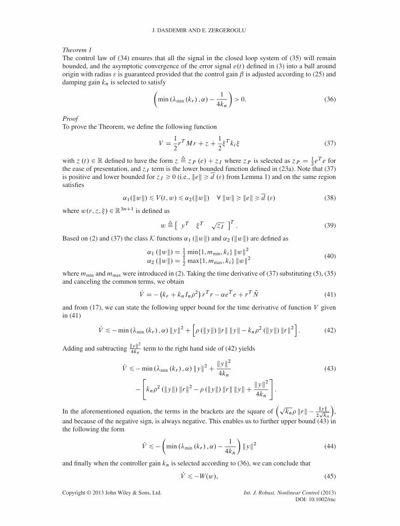
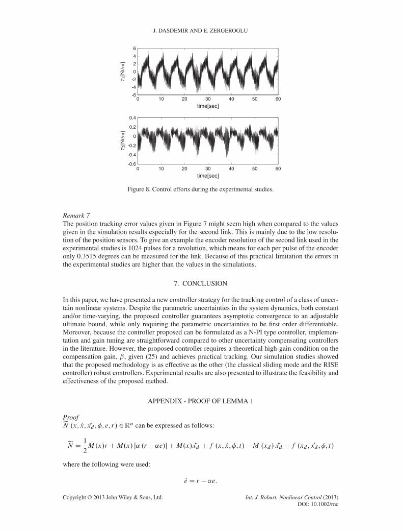
The tracking performance of the controller is illustrated in Figure 7, and the control efforts duringthe experiments are presented in Figure 8.



6

4

0.4

0.2

0

-0.2

-0.4

-0.6

2

0

0 10 20 30 40 50 60

-2

-4

-6

time[sec]

0 10 20 30 40 50 60

time[sec]

1[N

t/m]

2[N

t/m]

Figure 8. Control efforts during the experimental studies.

Remark 7The position tracking error values given in Figure 7 might seem high when compared to the valuesgiven in the simulation results especially for the second link. This is mainly due to the low resolu-tion of the position sensors. To give an example the encoder resolution of the second link used in theexperimental studies is 1024 pulses for a revolution, which means for each per pulse of the encoderonly 0.3515 degrees can be measured for the link. Because of this practical limitation the errors inthe experimental studies are higher than the values in the simulations.

7. CONCLUSION

In this paper, we have presented a new controller strategy for the tracking control of a class of uncer-tain nonlinear systems. Despite the parametric uncertainties in the system dynamics, both constantand/or time-varying, the proposed controller guarantees asymptotic convergence to an adjustableultimate bound, while only requiring the parametric uncertainties to be first order differentiable.Moreover, because the controller proposed can be formulated as a N-PI type controller, implemen-tation and gain tuning are straightforward compared to other uncertainty compensating controllersin the literature. However, the proposed controller requires a theoretical high-gain condition on thecompensation gain, ˇ, given (25) and achieves practical tracking. Our simulation studies showedthat the proposed methodology is as effective as the other (the classical sliding mode and the RISEcontroller) robust controllers. Experimental results are also presented to illustrate the feasibility andeffectiveness of the proposed method.

APPENDIX - PROOF OF LEMMA 1

ProofeN .x, Px, Rxd ,�, e, r/ 2Rn can be expressed as follows:

eN D 1

2PM.x/r CM.x/ Œ˛ .r � ˛e/�CM.x/ Rxd C f .x, Px,�, t /�M .xd / Rxd � f .xd , Pxd ,�, t /

where the following were used:

Pe D r � ˛e.



Let N .x, Px, Rxd ,�, e, r/ 2Rn be defined as

N WD1

2PM.x/r CM.x/ Rxd CM˛r �M˛

2eC f .x, Px,�, t / .

The auxiliary error eN.t/ can be written as the sum of errors pertaining to each of its arguments asfollows eN.t/D N .x, Px, Rxd ,�, e, r/�N .xd , Pxd , Rxd ,�, 0, 0/

D N .x, Pxd , Rxd ,�, 0, 0/�N .xd , Pxd , Rxd ,�, 0, 0/

CN .x, Px, Rxd ,�, 0, 0/�N .x, Pxd , Rxd ,�, 0, 0/

CN .x, Px, Rxd ,�, 0, 0/�N .x, Px, Rxd ,�, 0, 0/

CN .x, Px, Rxd ,�, 0, 0/�N .x, Px, Rxd ,�, 0, 0/

CN .x, Px, Rxd ,�, e, 0/�N .x, Px, Rxd ,�, 0, 0/

CN .x, Px, Rxd ,�, e, r/�N .x, Px, Rxd ,�, e, 0/

Applying the mean value theorem to eN.t/ results in the following expression:

eN.t/D@N .�1, Pxd , Rxd ,�, 0, 0/

@�1j�1D�1 .x � xd /

C@N .x, �2, Rxd ,�, 0, 0/

@�2j�2D�2 . Px � Pxd /

C@N .x, Px, �3,�, 0, 0/

@�3j�3D�3 . Rxd � Rxd /

C@N .x, Px, Rxd , �4, 0, 0/

@�4j�4D�4 .� � �/

C@N .x, Px, Rxd ,�, �5, 0/

@�5j�5D�5 e

C@N .x, Px, Rxd ,�, e, �6/

@�6j�6D�6 r

(A1)

where

�1 2 .xd , x/ , �2 2 . Pxd , Px/

�3 2 . Rxd , Rxd / , �4 2 .�,�/

�5 2 .0, e/ , �6 2 .0, r/

From (A1), eN.t/ can be upper bounded as follows:

keN.t/k6 ��@N .�1, Pxd , Rxd ,�, 0, 0/

@�1j�1D�1

�� kekC

��@N .x, �2, Rxd ,�, 0, 0/

@�2j�2D�2

�� kr � ˛ekC

��@N .x, Px, Rxd ,�, �5, 0/

@�5j�5D�5

�� kekC

��@N .x, Px, Rxd ,�, e, �6/

@�6j�6D�6

�� krk(A2)

by noting that

�1 Dx � c1 .x � xd /

�2 DPx � c2 . Px � Pxd /

�5 De .1� c5/

�6 Dr .1� c6/



where ci 2 .0, 1/ 2 R, i D 1, 2, 5, 6 are unknown constants, the following upper bound can bedeveloped ��@N .�1, Pxd , Rxd ,�, 0, 0/

@�1j�1D�1

��6�1.e/��@N .x, �2, Rxd ,�, 0, 0/

@�2j�2D�2

��6�2 .e, r/��@N .x, Px, Rxd ,�, �5, 0/

@�5j�5D�5

��6�5 .e, r/��@N .x, Px, Rxd ,�, e, �6/

@�6j�6D�6

��6�6 .e, r/

The bound on eN.t/ can be further reduced to

keN.t/k6 �1 .e/ kekC �2 .e, r/ kr � ˛ekC �5 .e, r/ kekC �6 .e, r/ krk. (A3)

Using the inequality

kr � ˛ek6 krkC ˛kek,

the expression in (A3) can be further upper bounded as follows:

keN.t/k6 Œ�1 .e/C ˛�2 .e, r/C �5 .e, r/� kekC Œ�2 .e, r/C �6 .e, r/� krk

Using the definition of y.t/ 2R2n, eN.t/ can be expressed in terms of y.t/ as follows:

keN.t/6 Œ�1 .e/C ˛�2 .e, r/C �5 .e, r/� ky.t/kC Œ�2 .e, r/C �6 .e, r/� ky.t/k

Therefore

keN.t/k6 � .kyk/ kykwhere � .kyk/ 2R1, explicitly defined as

� .kyk/> �1.e/C ˛�2 .e, r/C �5 .e, r/C �2 .e, r/C �6 .e, r/

is some positive bounding function that is assumed to be nondecreasing in ky.t/k. �

REFERENCES

1. Sastry S, Bodson M. Adaptive Control: Stability, Convergence and Robustness. Prentice Hall: Upper Saddle River,NJ, 1989.

2. Krstic M, Kanellakopoulos I, Kokotovic P. Nonlinear and Adaptive Control Design. John Wiley and Sons, Inc.:NewYork, 1995.

3. MacKunis W, Wilcox ZD, Kaiser MK, Dixon WE. Global adaptive output feedback tracking control of an unmannedaerial vehicle. IEEE Transactions on Control Systems Technology 2010; 18(6):1390–1397.

4. Ioannou PA, Sun J. Stable and Robust Adaptive Control. Prentice-Hall: Uppper Saddle River, NJ, 1996.5. Annaswanny A, Skantze F, Loh A. Adaptive control of continuous-time systems with convex/concave parametriza-

tions. Automatica Colaneri 1998; 34(1):33–49.6. Lin W, Qian C. Adaptive control of nonlinearly parameterized systems: a nonsmooth feedback framework. IEEE

Transactions on Automatic Control May 2002; 47:757–774.7. Qu Z, Hull RA, Wang J. Globally stabilizing adaptive control design for nonlinearly-parameterized systems. IEEE

Transactions on Automatic Control 2006; 51:1073–1079.8. Qu Z. Robust Control of Nonlinear Uncertain Systems, Wiley Series in Nonlinear Science, John Wiley and Sons, Inc.:

New York, USA, 1998.9. Bartolini G, Punta E, Zolezzi T. Simplex methods for nonlinear uncertain sliding-mode control. IEEE Transactions

on Automatic Control 2004; 49(6):922–933.10. Xu H, Ioannou PA. Robust adaptive control for a class of MIMO nonlinear systems with guaranteed error bounds.

IEEE Transactions on Automatic Control 2003; 48:728–742.11. Jiang ZP, Hill DJ. A robust adaptive backstepping scheme for nonlinear systems with unmodeled dynamics. IEEE

Transactions on Automatic Control 1999; 44:1705–1711.



12. Plycarpou MM, Ioannou PA. A robust adaptive nonlinear control design. Automatica 1995; 31:423–427.13. Yao B, Tomizuka M. Adaptive robust control of SISO nonlinear systems in a semi-strict feedback form. Automatica

1997; 33:893–900.14. Marino R, Tomei P. Robust adaptive state-feedback tracking for nonlinear systems. IEEE Transactions on Automatic

Control 1998; 43:84–89.15. Gee SS, Wang J. Robust adaptive tracking control for time-varying uncertain nonlinear systems with unknown control

coefficients. IEEE Transactions on Automatic Control 2003; 48:1463–1469.16. Lewis FL, Jagannathan S, Yesildirak A. Neural Network Control of Robot Manipulators and Nonlinar Systems.

Taylor and Francis: New York, 1999.17. Arimoto S, Kawamura S, Miyazaki F. Bettering operation of robots by learning. Journal of Robotic Systems 1984;

1(2):123–140.18. Messner W, Horowitz R, Kao WW, Boals M. A new adaptive learning rule. IEEE Transactions on Automatic Control

1991; 36(2):188–197.19. Dixon WE, Zergeroglu E, Dawson DM, Costic BT. Repetitive learning control: a lyapunov-based approach. IEEE

Transactions on Systems Man, and Cybernetics - Part B: Cybernetics August 2002; 32(4):538–545.20. Ortega R, Astolfi A, Barabanov NE. Nonlinear PI control of uncertain systems: an alternative to parameter adaptation.

Systems and Control Letters 2002; 47:259–278.21. Xian B, Dawson DM, de Queiroz MS, Chen J. A continuous asymptotic tracking control strategy for uncertain

nonlinear systems. IEEE Transactions on Automatic Control 2004; 49(7):1206–1211.22. Patre PM, Mackunis W, Makkar C, Dixon WE. Asymptotic tracking for systems with structured and unstructured

uncertainties. IEEE Transactions on Control Systems Technology 2008; 16(2):373–379.23. Makkar C, Hu G, Sawyer WG, Dixon WE. Lyapunov-based tracking control in the presence of uncertain nonlinear

parameterizable friction. IEEE Transactions on Automatic Control 2007; 52(10):1988–1994.24. Patre PM, MacKunis W, Kaiser K, Dixon WE. Asymptotic tracking for uncertain dynamic systems via a multilayer

neural network feedforward and rise feedback control structure. IEEE Transactions on Automatic Control 2008;53(9):2180–2185.

25. Dupree K, Patre P, Wilcox Z, Dixon WE. Asymptotic optimal control of uncertain nonlinear systems. Automatica2011; 47(1):99–107.

26. Slotine JJ, Li W. Applied Nonlinear Control. Prentice Hall: Englewood Cliff, NJ, 1991.27. Jiang ZP, Teel AR, Praly L. Small-gain theorem for ISS systems and applications. Mathematics Control Signals

Systems 1994; 7:95–120.28. Chaillet A, Loria A. Uniform global practical asymptotic stability for time-varying cascaded systems. European

Journal of Control 2006; 12(6):595–605.29. KHalil HK. Nonlinear Systems, 3rd ed. Prentice–Hall: Upper Saddle River, NJ, 2002.30. Direct Drive Manipulator Research and Development Package Operations Manual. Integrated Motion Inc.: Berkeley,

CA, 1992.


A new continuous high-gain controller scheme for a class of uncertain nonlinear systems

Documents

Transcript of A new continuous high-gain controller scheme for a class of uncertain nonlinear systems