A New Class of Generalized Power Lindley Distribution with ... 5_1_5.pdf · 54 A New Class of...

Theoretical Mathematics & Applications, vol.5, no.1, 2015, 53-96

ISSN: 1792-9687 (print), 1792-9709 (online)

Scienpress Ltd, 2015

A New Class of Generalized Power Lindley

Distribution with Applications to Lifetime Data

Mavis Pararai1, Gayan Warahena-Liyanage2 and Broderick O. Oluyede3

Abstract

A new class of distribution called the beta-exponentiated powerLindley (BEPL) distribution is proposed. This class of distributionsincludes the Lindley (L), exponentiated Lindley (EL), power Lindley(PL), exponentiated power Lindley (EPL), beta-exponentiated Lindley(BEL), beta-Lindley (BL), and beta-power Lindley distributions (BPL)as special cases. Expansion of the density of BEPL distribution is ob-tained. Some mathematical properties of the new distribution includinghazard function, reverse hazard function, moments, mean deviations,Lorenz and Bonferroni curves are presented. Entropy measures and thedistribution of the order statistics are given. The maximum likelihoodestimation technique is used to estimate the model parameters. Fi-nally, real data examples are discussed to illustrate the usefulness andapplicability of the proposed distribution.

Mathematics Subject Classification: 60E05; 62E15

1 Department of Mathematics, Indiana University of Pennsylvania, Indiana, PA, 15705,USA. E-mail: [email protected]

2 Department of Mathematics, Indiana University of Pennsylvania, Indiana, PA, 15705,USA. E-mail: [email protected]

3 Department of Mathematical Sciences, Georgia Southern University, Statesboro, GA,30460,USA. E-mail: [email protected]

Article Info: Received : August 7, 2014. Revised : September 19, 2014.Published online : January 10, 2015.

54 A New Class of Generalized Power Lindley Distribution

Keywords: Exponentiated power Lindley distribution; Power Lindley distri-

bution; Lindley distribution; Beta distribution; Maximum likelihood estima-

tion

1 Introduction

Lindley [1] developed Lindley distribution in the context of fiducial and

Bayesian statistics. Properties, extensions and applications of the Lindley

distribution have been studied in the context of reliability analysis by Ghitany

et al. [2], Zakerzadeh and Dolati [3], and Warahena-Liyanage and Pararai

[4]. Several other authors including Sankaran [5], Asgharzadeh et al. [6] and

Nadarajah et al. [7] proposed and developed the mathematical properties of

various generalized Lindley distributions. The probability density function

(pdf) of the Lindley distribution is given by

f(y; β) =β2

β + 1(1 + y)e−βy, y > 0, β > 0.

The power Lindley (PL) distribution proposed by Ghitany et al. [8] is an

extension of the Lindley (L) distribution. Using the transformation X = Y1α ,

Ghitany et al. [8] derived and studied the power Lindley (PL) distribution

with the probability density function (pdf) given by

f(x;α, β) =αβ2

β + 1(1 + xα)xα−1e−βxα

, x > 0, α > 0, β > 0.

The cumulative distribution function (cdf) of the power Lindley distribution

is

F (x) = 1− S(x) = 1−(

1 +βxα

β + 1

)e−βxα

for x > 0, α, β > 0. Warahena-Liyanage and Pararai [4] studied the properties

of the exponentiated Power Lindley (EPL) distribution. The EPL cdf and pdf

are given by

GEPL

(x;α, β, ω) =

[1−

(1 +

βxα

β + 1

)e−βxα

]ω

(1.1)

Mavis Pararai, Gayan Warahena-Liyanage and Broderick O. Oluyede 55

and

gEPL(x;α, β, ω) =αβ2ω


[1−

(1 +

βxα

β + 1

)e−βxα

]ω−1

,(1.2)

respectively, for x > 0, α > 0, β > 0, ω > 0. The hazard rate function of the

EPL distribution is given by

hGEPL(x;α, β, ω) =

g(x;α, β, ω)

G(x;α, β, ω)

=

αβ2ωβ+1

(1 + xα)xα−1e−βxα[1−

(1 + βxα

β+1

)e−βxα

]ω−1

1−[1−

(1 +

βxα

β + 1

)e−βxα

]ω .

The rth moment of the EPL distribution is given by

E(Xr) =∞∑i=0

i∑j=0

j+1∑k=0

(ω − 1

i

)(i

j

)(j + 1

k

)(−1)iβj−k−rα−1+1Γ(k + rα−1 + 1)

(β + 1)i+1(i+ 1)(k+rα−1+1).

The purpose of this paper is to develop a five-parameter alternative to

several lifetime distributions including the gamma, Weibull, exponentiated

Weibull, exponentiated Lindley, lognormal, beta Weibull geometric (BWG)

[9], and beta Weibull Poisson (BWP) [10] distributions. In this context, we

propose and develop the statistical properties of the beta exponentiated power

Lindley (BEPL) distribution and show that it is a competitive model for reli-

ability analysis. Our aim in this paper is to discuss some important statistical

properties of the BEPL distribution. This discussion includes the shapes of

the density, hazard rate and reverse hazard rate functions, moments, moment

generating function and parameter estimation by using the method of maxi-

mum likelihood. Finally, applications of the model to real data sets in order

to illustrate the applicability and usefulness of the BEPL distribution are pre-

sented.

This paper is organized as follows. In section 2, the model, sub-models and

some of its statistical properties including shapes and behavior of the hazard

function are presented. Moments, conditional moments, reliability and related

measures are given in section 3.Mean deviations, Bonferroni and Lorenz curves

are presented in section 4. Section 5 contains distribution of order statistics

and measures of uncertainty. In section 6, we present the maximum likelihood


method for estimating the parameters of the distribution. Applications are

given in section 7 followed by concluding remarks.

2 The Model, Sub-models and Some Proper-

ties

In this section, we present the BEPL distribution and derive some prop-

erties of this class of distributions including the cdf, pdf, expansion of the

density, hazard and reverse hazard functions, shape and sub-models. Let G(x)

denote the cdf of a continuous random variable X and define a general class

of distributions by

F (x) =BG(x)(a, b)

B(a, b), (2.1)

where BG(x)(a, b) =∫ G(x)

0ta−1(1 − t)b−1dt and 1/B(a, b) = Γ(a + b)/Γ(a)Γ(b).

The class of generalized distributions above was motivated by the work of Eu-

gene et al. [11]. They proposed and studied the beta-normal distribution.

Some beta-generalized distributions discussed in the literature include work

by Jones [12], Bidram et al. [9]. Nadarajah and Kotz [13], Nadarajah and

Gupta [14], Nadarajah and Kotz [15], Barreto-Souza et al. [16] proposed the

beta-Gumbel, beta-Frechet, beta-exponential (BE), beta-exponentiated expo-

nential (BEE) distributions, respectively. Gusmao et al. [17] presented results

on the generalized inverse Weibull distribution. Pescim et al. [18] proposed

and studied the beta-generalized half-normal distribution which contains some

important distributions such as the half-normal and generalized half normal

(Cooray and Ananda [19]) as special cases. Furthermore, Cordeiro et al. [20]

presented the generalized Rayleigh distribution and Carrasco et al. [21] stud-

ied the generalized modified Weibull distribution with applications to lifetime

data. More recently, Oluyede and Yang [22] studied the beta generalized Lind-

ley distribution with applications.

By considering G(x) as the cdf of EPL distribution we obtain the beta-

exponentiated power Lindley (BEPL) distribution with a broad class of dis-

tributions that may be applicable in a wide range of day to day situations


including applications in medicine, reliability and ecology. The cdf and pdf of

the five-parameter BEPL distribution are given by

FBEPL(x;α, β, ω, a, b) =1

B(a, b)

∫ GEPL(x;α,β,ω)

0

ta−1(1− t)b−1dt

=BG(x)(a, b)

B(a, b), (2.2)

and

fBEPL(x;α, β, ω, a, b) =1

B(a, b)[GEPL(x)]a−1 [1−GEPL(x)]b−1 gEPL(x),

=αβ2ω

B(a, b)(β + 1)(1 + xα)xα−1e−βxα

×[1−

(1 +

βxα

β + 1

)e−βxα

]ωa−1

×{

1−[1−

(1 +

βxα

β + 1

)e−βxα

]ω}b−1

, (2.3)

respectively, for x > 0, α > 0, β > 0, ω > 0, a > 0, b > 0. Plots of the pdf

of BEPL distribution for several combinations of values of α, β, ω, a and b are

given in Figure 2.1. The plots indicate that the BEPL pdf can be decreasing

or right skewed. The BEPL distribution has a positive asymmetry.

Figure 2.1: Plots of the PDF for different values of α, β, ω, a and b

2.1 Expansion of density

The expansion of the pdf of BEPL distribution is presented in this section.


For b > 0 a real non-integer, we use the series representation

(1−GEPL(x))b−1 =∞∑i=0

(b− 1

i

)(−1)i [GEPL(x)]i, (2.4)

where

GEPL(x;α, β, ω) =

[1−

(1 +

βxα

β + 1

)e−βxα

]ω

.

If a is an integer, from Equation (2.3) and the above expansion (2.4), we

can rewrite the density of the BEPL distribution as

fBEPL(x;α, β, ω, a, b) =gEPL(x)

B(a, b)

∞∑i=0

(b− 1

i

)(−1)i [GEPL(x)]a+i−1 (2.5)

=αβ2ω


[1−

(1 +

βxα

β + 1

)e−βxα

]ω−1

×∞∑i=0

(−1)i(

b−1i

)B(a, b)

[1−

(1 +

βxα

β + 1

)e−βxα

]ω(a+i−1)

=αβ2ω


×∞∑i=0

li

[1−

(1 +

βxα

β + 1

)e−βxα

]ω(a+i)−1

, (2.6)

where the coefficients li are

li = li(a, b) =(−1)i

(b−1

i

)B(a, b)

and∑∞

i=0 li = 1, for x > 0, α > 0, β > 0, ω > 0, a > 0, b > 0.

If a is real non-integer, we can expand [GEPL(x)]a+i−1 as follows:

[GEPL(x)]a+i−1 = {1− [1−GEPL(x)]}a+i−1

=∞∑

j=0

(a+ i− 1

j

)(−1)j [1−GEPL(x)]j ,

with

[1−GEPL(x)]j =

j∑k=0

(j

k

)(−1)k [GEPL(x)]k ,


so that

[GEPL(x)]a+i−1 =∞∑

j=0

j∑k=0

(a+ i− 1

j

)(j

k

)(−1)j+k [GEPL(x)]k . (2.7)

From Equations (2.5) and (2.7), the BEPL density can be rearranged in the

form

fBEPL(x;α, β, ω, a, b) = gEPL(x)∞∑

i,j=0

j∑k=0

li,j,k [GEPL(x)]k (2.8)

=αβ2ω


)

×∞∑

i,j=0

j∑k=0

li,j,k

[1−

(1 +

βxα

β + 1

)e−βxα

]ω(k+1)−1

,

where the coefficients li,j,k are

li,j,k = li,j,k(a, b) =(−1)i+j+k

(b−1

i

)(a+i−1

j

)(jk

)B(a, b)

and∑∞

i,j=0

∑jk=0 li,j,k = 1, for x > 0, α > 0, β > 0, ω > 0, a > 0, b > 0. Hence,

for any real non-integer, the BEPL density is given by three (two infinite

and one finite) weighted power series sums of the baseline cdf GEPL(x). By

changing∑∞

j=0

∑jk=0 to

∑∞k=0

∑∞j=k in Equation (2.8), we obtain

fBEPL(x;α, β, ω, a, b) = gEPL(x)∞∑

i,k=0

pi [GEPL(x)]k

=αβ2ω


×∞∑

i,k=0

pi

[1−

(1 +

βxα

β + 1

)e−βxα

]ω(k+1)−1

,

where the coefficient pi is

pi = pi(a, b) =(−1)i

(b−1

i

)qk(a+ i− 1)

B(a, b),

with

qk = qk(a+ i− 1) =∞∑

j=k

(a+ i− 1

j

)(j

k

)(−1)j+k,


for x > 0, α > 0, β > 0, ω > 0, a > 0, b > 0, respectively. Note that the BEPL

density is given by three infinite weighted power series sums of the baseline

distribution function GEPL(x). When b > 0 is an integer, the index i in the

previous series representation stops at b− 1.

2.2 Some sub-models of the BEPL distribution

Some sub-models of the BEPL distribution for selected values of the pa-

rameters α, β, ω, a and b are presented in this section.

(1) a = b = 1

When a = b = 1, we obtain the exponentiated power Lindley (EPL)

distribution whose cdf and pdf are given in (1.1) and (1.2), (Warahena-

Liyanage and Pararai [4]).

(2) ω = 1

When ω = 1, we obtain the beta-power Lindley (BPL) distribution. The

BPL cdf is given by

FBPL(x;α, β, a, b) =1

B(a, b)

∫ GPL(x;α,β)

0


for x > 0, α > 0, β > 0, a > 0, b > 0. The corresponding pdf is given by

fBPL(x;α, β, a, b) =αβ2

B(a, b)(β + 1)(1 + xα)xα−1e−βxα

×[1−

(1 +

βxα

β + 1

)e−βxα

]a−1[(1 +

βxα

β + 1

)e−βxα

]b−1

for x > 0, α > 0, β > 0, a > 0, b > 0.

(3) α = 1

When α = 1, we obtain beta-exponentiated Lindley (BEL) distribution

(Oluyede and Yang [22]). The BEL cdf is given by

FBEL(x; β, ω, a, b) =1

B(a, b)

∫ GEL(x;β,ω)

0



for x > 0, β > 0, ω > 0, a > 0, b > 0. The corresponding pdf is given by

fBEL(x; β, ω, a, b) =β2ω

B(a, b)(β + 1)(1 + x)e−βx

×[1−

(1 +

βx

β + 1

)e−βx

]ωa−1

×{

1−[1−

(1 +

βx

β + 1

)e−βx

]ω}b−1

for x > 0, β > 0, ω > 0, a > 0, b > 0.

(4) ω = α = 1

When ω = α = 1, we obtain beta-Lindley (BL) distribution (Oluyede

and Yang [22]). The BL cdf and pdf are given by

FBL(x; β, a, b) =1

B(a, b)

∫ GL(x;β,ω)

0


and

fBL(x; β, a, b) =β2

B(a, b)(β + 1)(1 + x)e−βx

×[1−

(1 +

βx

β + 1

)e−βx

]a−1[(1 +

βx

β + 1

)e−βx

]b−1

,

respectively, for x > 0, β > 0, ω > 0, a > 0, b > 0.

(5) ω = a = b = 1

When ω = a = b = 1, we obtain the power Lindley (PL) distribution

(Ghitany et al. [8]). The PL cdf and pdf are respectively given by

FPL(x;α, β) = 1−(

1 +βxα

β + 1

)e−βxα

and

fPL(x;α, β) =β2

(β + 1)(1 + xα)xα−1e−βxα

for x > 0, α > 0, β > 0.


(6) α = a = b = 1

When α = a = b = 1, we obtain exponentiated-Lindley (EL) distribu-

tion. The EL cdf is given by

FEL(x; β, ω) =

[1−

(1 +

βx

β + 1

)e−βx

]ω

for x > 0, β > 0, ω > 0. The corresponding pdf is given by

fEL(x; β, ω) =β2ω

(β + 1)(1 + x)e−βx

[1−

(1 +

βx

β + 1

)e−βx

]ω−1

for x > 0, β > 0, ω > 0.

(7) α = ω = a = b = 1

When α = ω = a = b = 1, we obtain Lindley distribution. The Lindley

cdf and pdf are respectively given by

FL(x; β) = 1−(

1 +βx

β + 1

)e−βx

and

fL(x; β) =β2

(β + 1)(1 + x)e−βx

for x > 0, β > 0.

(8) ω = a = 1

When ω = a = 1, the cdf of BEPL distribution reduces to

FBPL(x;α, β, b) = 1−[(

1 +βxα

β + 1

)e−βxα

]b

for x > 0, α > 0, β > 0, b > 0. The corresponding pdf is

fBPL(x;α, β, b) =bαβ2

(β + 1)(1 + xα)xα−1e−βxα

[(1 +

βxα

β + 1

)e−βxα

]b−1

for x > 0, α > 0, β > 0, b > 0.

(9) α = a = 1

When α = a = 1, the cdf of BEPL distribution reduces to

FBEL(x;α, β, b) = 1−{

1−[1−

(1 +

βx

β + 1

)e−βx

]ω}b


for x > 0, β > 0, ω > 0, b > 0. The corresponding pdf is given by

fBEL(x; β, ω, b) =bωβ2

(β + 1)(1 + x)e−βx

×[1−

(1 +

βx

β + 1

)e−βx

]ω−1

×{

1−[1−

(1 +

βx

β + 1

)e−βx

]ω}b−1

,

for x > 0, β > 0, ω > 0, b > 0. This is the Kumaraswamy Lindley

distribution with parameters β, ω and b.

(10) α = ω = a = 1

When α = ω = a = 1, the cdf of BEPL distribution reduces to

FBL(x; β, b) = 1−[(

1 +βx

β + 1

)e−βx

]b

for x > 0, β > 0, b > 0. The corresponding pdf is given by

fBL(x; β, b) =bβ2

(β + 1)(1 + x)e−βx

[(1 +

βx

β + 1

)e−βx

]b−1

for x > 0, β > 0, b > 0.

2.3 Hazard and Reverse Hazard Functions

The hazard and reverse hazard functions of the BEPL distribution are

presented in this section. Graphs of these functions for selected values of

parameters α, β, ω, a and b are also presented. The hazard and reverse hazard

functions of the BEPL distribution are given respectively by

hBEPL(x;α, β, ω, a, b) =fBEPL(x;α, β, ω, a, b)

FBEPL(x;α, β, ω, a, b)

=gEPL(x) [GEPL(x)]a−1 [1−GEPL(x)]b−1

B(a, b)−BGEPL(x)(a, b)

and


τBEPL(x;α, β, ω, a, b) =fBEPL(x;α, β, ω, a, b)

FBEPL(x;α, β, ω, a, b)

=gEPL(x) [GEPL(x)]a−1 [1−GEPL(x)]b−1

BGEPL(x)(a, b),

for x > 0, α > 0, β > 0, ω > 0, a > 0, b > 0, where GEPL(x) and gEPL(x) are

the cdf and pdf of the EPL distribution given by Equations (1.1) and (1.2),

respectively. Plots of the hazard function for selected values of parameters

α, β, ω, a and b are given in Figures 2.2 and 2.3. The graphs of the hazard

function for several combinations of the parameters represent various shapes

including monotonically increasing, monotonically decreasing, bathtub and up-

side down bathtub shapes. This attractive flexibility makes BEPL hazard

rate function useful and suitable for non-monotone empirical hazard behaviors

which are more likely to be encountered or observed in real life situations.

Figure 2.2: Plots of the hazard function for different values of α, β, ω, a and b

2.4 Monotonicity Properties

The monotonicity properties of the BEPL distribution are discussed in this

section. Let

V (x) = GPL(x;α, β) = 1−(

1 +βxα

β + 1

)e−βxα

.


Figure 2.3: Plots of the hazard function for different values of α, β, ω, a and b

From Equation (2.3) we can rewrite the BEPL pdf as

fBEPL(x;α, β, ω, a, b) =αβ2ω

B(a, b)(β + 1)(1 + xα)xα−1e−βxα

× [V (x)]ωa−1[1− V ω(x)]b−1

for x > 0, α > 0, β > 0, ω > 0, a > 0, b > 0. It follows that

log fBEPL(x) = log

(αβ2ω

B(a, b)(β + 1)

)+ log(1 + xα) + (α− 1) log(x)− βxα

+ (ωa− 1) log V (x) + (b− 1) log [1− V α(x)] , (2.9)

and

d log fBEPL(x)

dx=

αxα−1

1 + xα+α− 1

x− αβxα−1

+(ωa− 1)(1− V ω(x))− ω(b− 1)V ω(x)

V (x) [1− V ω(x)]V ′(x).

(2.10)

Substituting V ′(x) = dV (x)/dx = (αβ2/(β + 1))(1 + xα)xα−1e−βxαinto Equa-

tion (2.10), we have

d log fBEPL(x)

dx=

αxα−1

1 + xα+α− 1

x− αβxα−1 +

αβ2


×{

(ωa− 1)(1− V ω(x))− ω(b− 1)V ω(x)

V (x) [1− V ω(x)]

}.


Since α > 0, β > 0, ω > 0, a > 0 and b > 0, we have

V ′(x) =dV (x)

dx=

αβ2


> 0,∀x > 0. (2.11)

If x −→ 0, then

V (x) = 1−(

1 +βxα

β + 1

)e−βxα −→ 0.

If x −→∞, then

V (x) = 1−(

1 +βxα

β + 1

)e−βxα −→ 1.

Thus V (x) is monotonically increasing from 0 to 1. Note that, since 0 <

V (x) < 1,

0 < V ω(x) < 1,∀ω > 0, 0 < 1 − V ω(x) < 1,∀ω > 0 and V ′(x) > 0, we have

V ′(x)/V (x)[1− V ω(x)] > 0.

If α 6 1/2, ωa < 1 and b > 1. we obtain

d log fBEPL(x)

dx=

αxα−1

1 + xα+α− 1

x− αβxα−1

+(ωa− 1)(1− V ω(x))− ω(b− 1)V ω(x)

V (x) [1− V ω(x)]V ′(x) < 0

(2.12)

since [αxα−1/(1 + xα)] + [(α− 1)/x] = [(2α− 1)xα + (α− 1)]/x(1 + xα) < 0,

(ωa− 1)(1− V ω(x))− ω(b− 1)V ω(x) < 0 and V ′(x)/V (x)[1− V ω(x)] > 0.

In this case, fBEPL(x;α, β, ω, a, b) is monotonically decreasing for all x.

If α > 1/2, fBEPL(x;α, β, ω, a, b) could attain a maximum, a minimum or a

point of inflection according to whether

d2 log fBEPL(x)

dx2< 0,

d2 log fBEPL(x)

dx2> 0 or

d2 log fBEPL(x)

dx2= 0.

3 Moments, Conditional Moments and Relia-

bility

In this section, moments, conditional moments and reliability and related

measures including coefficients of variation, skewness and kurtosis of the BEPL


distribution are presented. A table of values for mean, variance, coefficient of

skewness (CS) and coefficient of kurtosis (CK) is also presented.

3.1 Moments

The rth moment of the BEPL distribution, denoted by µ′r is given by

µ′r = E(Xr) =

∫ ∞

−∞xrf

BEPL(x)dx for r = 0, 1, 2, . . . .

In order to find the moments of the BEPL distribution, consider the following

lemma.

Lemma 3.1. Let

L1(α, β,m, r) =

∫ ∞

0

(1 + xα)xα+r−1

[1−

(1 +

βxα

β + 1

)e−βxα

]m−1

e−βxα

dx,

then

L1(α, β,m, r) =∞∑

j=0

j∑k=0

k+1∑l=0

(m− 1

j

)(j

k

)(k + 1

l

)(−1)jβkΓ(l + rα−1 + 1)

α(β + 1)j [β(j + 1)](l+rα−1+1).

Proof. Using the series expansion

(1− z)a−1 =∞∑i=0

(a− 1

i

)(−1)izi, (3.1)

where | z |< 1 and b > 0 is a real non-integer, we have

L1(α, β,m, r) =∞∑

j=0

(m− 1

j

)(−1)j

∫ ∞

0

[1 + β(1 + xα)

β + 1

]j

e−jβxα

(1 + xα)xα+r−1e−βxα

dx

=∞∑

j=0

(m− 1

j

)(−1)j

(β + 1)j

j∑k=0

(j

k

)βk

∫ ∞

0

(1 + xα)k+1xα+r−1e(−jβxα−βxα)dx

=∞∑

j=0

(m− 1

j

) j∑k=0

(j

k

) k+1∑l=0

(k + 1

l

)(−1)jβk

(β + 1)j

∫ ∞

0

xα+αl+r−1e(−jβxα−βxα)dx.


Now consider, ∫ ∞

0

xα+αl+r−1e(−jβxα−βxα)dx. (3.2)

Let u = β(j + 1)xα, then dudx

= αβ(j + 1)xα−1 and x =

[u

β(j + 1)

]1/α

.

Consequently,

L1(α, β,m, r) =∞∑

j=0

j∑k=0

k+1∑l=0

(m− 1

j

)(j

k

)(k + 1

l

)(−1)jβkΓ(l + rα−1 + 1)

α(β + 1)j [β(j + 1)](l+rα−1+1).

Therefore, the rth moment of the BEPL distribution from equation (2.6) is

given by

µ′r =αβ2ω

B(a, b)(β + 1)

∞∑i=0

(b− 1

i

)(−1)i

×∫ ∞

0

xr(1 + xα)xα−1

[1−

(1 +

βxα

β + 1

)e−βxα

]ω(a+i)−1

e−βxα

dx.

Now, using Lemma 3.1 with m = ω(a+ i), we have

µ′r =αβ2ω

B(a, b)(β + 1)

∞∑i=0

(b− 1

i

)(−1)iL1(α, β, ω(a+ i), r). (3.3)

The mean, variance, coefficient of variation (CV), coefficient of skewness (CS)

and coefficient of kurtosis (CK) are given by

µ = µ′1 =αβ2ω

B(a, b)(β + 1)

∞∑i=0

(b− 1

i

)(−1)iL1(α, β, ω(a+ i), 1), (3.4)

σ2 = µ′2 − µ2, (3.5)

CV =σ

µ=

√µ′2 − µ2

µ=

√µ′2µ2− 1, (3.6)

CS =E [(X − µ)3]

[E(X − µ)2]3/2=µ′3 − 3µµ′2 + 2µ3

(µ′2 − µ2)3/2, (3.7)

and

CK =E [(X − µ)4]

[E(X − µ)2]2=µ′4 − 4µµ′3 + 6µ2µ′2 − 3µ4

(µ′2 − µ2)2, (3.8)


respectively.

Table 3.1 lists the first six moments of the BEPL distribution for selected

values of the parameters by fixing α = 1.5, β = 1.0 and ω = 1.5. These values

can be determined numerically using R and MATLAB. Algorithms to calcu-

late the pdf moments, reliability, mean deviations, Renyi entropy, maximum

likelihood estimators and variance-covariance matrix of the BEPL distribution

are provided in the appendix.

Table 3.1: Moments of the BEPL distribution for some parameter values;

α = 1.5, β = 1.0 and ω = 1.5

µ′s a = 0.5, b = 1.5 a = 1.5, b = 1.5 a = 1.5, b = 2.5 a = 2.5, b = 1.5

µ′1 0.8348214 1.407729 1.129684 1.685774

µ′2 1.035256 2.304562 1.472533 3.13659

µ′3 1.608199 4.258207 2.149913 6.366501

µ′4 2.928858 8.712316 3.450266 13.97437

µ′5 6.037089 19.4759 6.007677 32.94413

µ′6 13.77834 47.09621 11.24152 82.9509

Variance 0.33832923 0.322861063 0.19634706 0.294756021

Skewness 0.90987141 0.572390725 0.491885701 0.532003392

Kurtosis 3.760808259 3.40572536 3.236667109 3.434460209

3.2 Conditional Moments

For lifetime models, it is useful to know the conditional moments defined

as E(Xr | X > x). In order to calculate the conditional moments, we consider

the following lemma:

Lemma 3.2. Let

L2(α, β,m, r, t) =

∫ ∞

t

(1 + xα)xα+r−1

[1−

(1 +

βxα

β + 1

)e−βxα

]m−1

e−βxα

dx.

then

L2(α, β,m, r, t) =∞∑

j=0

j∑k=0

k+1∑l=0

(m− 1

j

)(j

k

)(k + 1

l

)(−1)jβkΓ(l + rα−1 + 1, β(j + 1)tα)

α(β + 1)j [β(j + 1)](l+rα−1+1),


where Γ(a, t) =∫∞

txa−1s−xdx is the upper incomplete gamma function.

Proof. Using the same procedure that was used in Lemma 3.1, this can be

simplified into the following form.

L2(α, β,m, r, t) =∞∑

j=0

j∑k=0

k+1∑l=0

(m− 1

j

)(j

k

)(k + 1

l

)(−1)jβk

(β + 1)j(3.9)

×∫ ∞

t

xα+αl+r−1e(−jβxα−βxα)dx. (3.10)

Now consider,∫∞

txα+αl+r−1e(−jβxα−βxα)dx, and let u = β(j + 1)xα, then

dudx

= αβ(j + 1)xα−1 and x =

[u

β(j + 1)

]1/α

. The above integral can be rewrit-

ten by using the complementary incomplete gamma function Γ(a, t) =∫∞

txa−1e−xdx.

Consequently,

L2(α, β,m, r, t) =∞∑

j=0

j∑k=0

k+1∑l=0

(m− 1

j

)(j

k

)(k + 1

l

)(−1)jβkΓ(l + rα−1 + 1, β(j + 1)tα)

α(β + 1)j [β(j + 1)](l+rα−1+1).

Now using Lemma 3.2, the rth conditional moment of the BEPL distribution

is given by

E(Xr|X > x) =αβ2ω

B(a, b)(β + 1)

∞∑i=0

(b− 1

i

)(−1)i L2(α, β, ω(a+ i), r, x)

1− FBEPL(x;α, β, ω, a, b)

=αβ2ω

(β + 1)

∞∑i=0

(b− 1

i

)(−1)i L2(α, β, ω(a+ i), r, x)

B(a, b)−BGELP (x)(a, b).

The mean residual lifetime function is given by E(X|X > x)−x. The moment

generating function (MGF) of the BEPL distribution is given by

MX(t) =αβ2ω

B(a, b)(β + 1)

∞∑i=0

∞∑n=0

(b− 1

i

)(−1)i t

n

n!L1(α, β, ω(a+ i), n). (3.11)

3.3 Reliability

We derive the reliabilityR whenX and Y have independent BEPL(α1, β1, ω1, a1, b1)

and BEPL(α2, β2, ω2, a2, b2) distributions, respectively. Note from Equation


(2.2) that the BEPL cdf can be written as:

FBEPL(x;α, β, ω, a, b) =1

B(a, b)

∫ GEPL(x;α,β,ω)

0

ta−1(1− t)b−1dt,

=1

B(a, b)

∞∑j=0

(b− 1

j

)(−1)j

a+ j

[1−

(1 +

βxα

β + 1

)e−βxα

]ω(a+j)

.

(3.12)

Now, from Equations (3.12) and (2.3), we obtain

R = P (X > Y )

=

∫ ∞

0

fX(x;α1, β1, ω1, a1, b1)FY (x;α2, β2, ω2, a2, b2)dx

=

∫ ∞

0

α1β21ω1

B(a1, b1)(β1 + 1)(1 + xα1)xα1−1e−β1xα1

×[1−

(1 +

β1xα1

β1 + 1

)e−β1xα1

]ω1a1−1

×{

1−[1−

(1 +

β1xα1

β1 + 1

)e−β1xα1

]ω1}b1−1

× 1

B(a2, b2)

∞∑j=0

(b2 − 1

j

)(−1)j

a2 + j

[1−

(1 +

β2xα2

β2 + 1

)e−β2xα2

]ω2(a2+j)

dx.

(3.13)

We apply the following series representations:[1−

(1 +

β1xα1

β1 + 1

)e−β1xα1

]ω1a1−1

=∞∑

k=0

(ω1a1 − 1

k

)(−1)k

(1 +

β1xα1

β1 + 1

)k

e−β1kxα1

=∞∑

k=0

k∑m=0

(ω1a1 − 1

k

)(k

m

)(−1)kβm

1 xmα1

(β1 + 1)me−β1kxα1 ,

(3.14)

{1−

[1−

(1 +

β1xα1

β1 + 1

)e−β1xα1

]ω1}b1−1

=∞∑l=0

∞∑p=0

p∑n=0

(b1 − 1

l

)(ω1l

p

)(p

n

)× (−1)l+pβn

1 xnα1

(β1 + 1)ne−β1pxα1 (3.15)


and[1−

(1 +

β2xα2

β2 + 1

)e−β2xα2

]ω2(a2+j)

=∞∑

q=0

q∑t=0

(ω2(a2 + j)

q

)(q

t

)(−1)qβt

2xtα2

(β2)te−β2qxα2 .

(3.16)

By substituting Equations (3.14), (3.15) and (3.16) into Equation (3.13), we

obtain

R =

∫ ∞

0

α1β21ω1

B(a1, b1)(β1 + 1)(1 + xα1)xα1−1e−β1xα1

×∞∑

k=0

k∑m=0

(ω1a1 − 1

k

)(k

m

)(−1)kβm

1 xmα1

(β1 + 1)me−β1kxα1

×∞∑l=0

∞∑p=0

p∑n=0

(b1 − 1

l

)(ω1l

p

)(p

n

)(−1)l+pβn

1 xnα1

(β1 + 1)ne−β1pxα1

× 1

B(a2, b2)

∞∑j=0

(b2 − 1

j

)(−1)j

a2 + j

×∞∑

q=0

q∑t=0

(ω2(a2 + j)

q

)(q

t

)(−1)qβt

2xtα2

(β2)te−β2qxα2dx

=α1ω1

B(a1, b1)B(a2, b2)

∞∑k,l,p,j,q=0

k∑m=0

p∑n=0

q∑t=0

(ω1a1 − 1

k

)(k

m

)(b1 − 1

l

)(ω1l

p

)

×(p

n

)(b2 − 1

j

)(ω2(a2 + j)

q

)(q

t

)(−1)k+l+p+j+qβm+n+2

1 βt2

(β1 + 1)m+n+1(β2 + 1)t(a2 + j)

×∫ ∞

0

(1 + xα1)x(m+n+1)α1+tα2−1exp(− [β1(1 + p+ k)xα1 + β2qxα2 ])dx.

(3.17)

Note that,∫ ∞

0

(1 + xα1)x(m+n+1)α1+tα2−1

×e−β1(1+p+k)xα1−β2qxα2dx =∞∑

s=0

∞∑r=0

(α1

r

)(−1)sβs

1(1 + p+ k)s

×∫ ∞

0

x(m+n+s+1)α1+tα2+r−1e−β2qxα2dx.

(3.18)


Using the definition of gamma function, we have∞∫

0

x(m+n+s+1)α1+tα2+r−1e−β2qxα2dx =Γ((m+ n+ s+ 1)α1α

−12 + rα−1

2 + t)

α2(β2q)(m+n+s+1)α1α−12 +rα−1

2 +t.

(3.19)

Substituting Equation (3.19) into Equation (3.18), we obtain∫ ∞

0

(1 + xα1)x(m+n+1)α1+tα2−1

×e−β1(1+p+k)xα1−β2qxα2dx =∞∑

s=0

∞∑r=0

(α1

r

)(−1)sβs

1(1 + p+ k)s

× Γ((m+ n+ s+ 1)α1α−12 + rα−1

2 + t)

α2(β2q)(m+n+s+1)α1α−12 +rα−1

2 +t.

(3.20)

Finally, substituting Equation (3.20) into (3.17), we obtain

R =α1ω1

B(a1, b1)B(a2, b2)

∞∑k,l,p,j,q=0

k∑m=0

p∑n=0

q∑t=0

(ω1a1 − 1

k

)(k

m

)(b1 − 1

l

)(ω1l

p

)

×(p

n

)(b2 − 1

j

)(ω2(a2 + j)

q

)(q

t

)(−1)k+l+p+j+qβm+n+2

1 βt2

(β1 + 1)m+n+1(β2 + 1)t(a2 + j)

×∞∑

s=0

∞∑r=0

(α1

r

)(−1)sβs

1(1 + p+ k)s

× Γ((m+ n+ s+ 1)α1α−12 + rα−1

2 + t)

α2(β2q)(m+n+s+1)α1α−12 +rα−1

2 +t.

=α1ω1

B(a1, b1)B(a2, b2)

∞∑k,l,p,j,q,s,r=0

k∑m=0

p∑n=0

q∑t=0

(ω1a1 − 1

k

)(k

m

)(b1 − 1

l

)(ω1l

p

)

×(p

n

)(b2 − 1

j

)(ω2(a2 + j)

q

)(q

t

)(α1

r

)(−1)k+l+p+j+q+sβm+n+s+2

1 βt2(1 + p+ k)s

(β1 + 1)m+n+1(β2 + 1)t(a2 + j)

× Γ((m+ n+ s+ 1)α1α−12 + rα−1

2 + t)

α2(β2q)(m+n+s+1)α1α−12 +rα−1

2 +t.

4 Mean Deviations, Bonferroni and Lorenz Curves

In this section, we present the mean deviation about the mean, the mean

deviation about the median, Bonferroni and Lorenz curves. Bonferroni and


Lorenz curves are income inequality measures that are also useful and appli-

cable in other areas including reliability, demography, medicine and insurance.

The mean deviation about the mean and mean deviation about the median

are defined by

D(µ) =

∫ ∞

0

| x− µ | f(x)dx and D(M) =

∫ ∞

0

| x−M | f(x)dx,

respectively, where µ = E(X) and M = Median(X) = F−1(1/2) is the median

of F. These measuresD(µ) andD(M) can be calculated using the relationships:

D(µ) = 2µF (µ)− 2µ+ 2

∫ ∞

µ

xf(x)dx = 2µF (µ)− 2

∫ µ

0

xf(x)dx,

and

D(M) = −µ+ 2

∫ ∞

M

xf(x)dx = µ− 2

∫ M

0

xf(x)dx.

Now using Lemma 3.2, we have

D(µ) = 2µFBEPL(µ)− 2µ+2αβ2ω

B(a, b)(β + 1)

∞∑i=0

(b− 1

i

)(−1)iL2(α, β, ω(a+ i), 1, µ)

and

D(M) = −µ+2αβ2ω

B(a, b)(β + 1)

∞∑i=0

(b− 1

i

)(−1)iL2(α, β, ω(a+ i), 1,M).

Lorenz and Bonferroni curves are given by

L(FBEPL

(x)) =

∫ x

0xf

BEPL(x)dx

E(X), and B(F

BEPL(x)) =

L(FBEPL

(x))

FBEPL

(x),

or

L(p) =1

µ

∫ q

0

xfBEPL

(x)dx, and B(p) =1

pµ

∫ q

0

xfBEPL

(x)dx,

respectively, where q = F−1BEPL

(p). Using Lemma 3.2, we can re-write Lorenz

and Bonferroni curves as

B(p) =1

pµ

∫ q

0

xfBEPL(x)dx

=1

pµ

[∫ ∞

0

xfBEPL

(x)dx−∫ ∞

q

xfBEPL

(x)dx

]=

1

pµ

[µ− αβ2ω

B(a, b)(β + 1)

∞∑i=0

(b− 1

i

)(−1)iL2(α, β, ω(a+ i), 1, q)

],


and

L(p) =1

µ

∫ q

0

xfBEPL(x)dx

=1

µ

[∫ ∞

0

xfBEPL

(x)dx−∫ ∞

q

xfBEPL

(x)dx

]=

1

µ

[µ− αβ2ω

B(a, b)(β + 1)

∞∑i=0

(b− 1

i

)(−1)iL2(α, β, ω(a+ i), 1, q)

].

5 Order Statistics and Measures of Uncertainty

In this section, we present distribution of order statistics, Shannon entropy

[23], [24], as well as Renyi entropy [25] for the BEPL distribution. The concept

of entropy plays a vital role in information theory. The entropy of a random

variable is defined in terms of its probability distribution and is a good measure

of randomness or uncertainty.

5.1 Distribution of Order Statistics

Order Statistics play an important role in probability and statistics. In

this section, we present the distribution of the order statistics for the BEPL

distribution. Suppose that X1, X2, . . . , Xn is a random sample of size n from a

continuous pdf, f(x). Let X1:n < X2:n < . . . < Xn:n denote the corresponding

order statistics. If X1, X2, . . . , Xn is a random sample from BEPL distribution,

it follows from Equations (2.2) and (2.3) that the pdf of the kth order statistic,

say Yk = Xk:n is given by

fk(yk) =n!

(k − 1)!(n− k)!f

BEPL(yk)

n−k∑l=0

(n− k

l

)(−1)l

[BGEPL(yk;α,β,ω)(a, b)

B(a, b)

]k+l−1

× αβ2ω

B(a, b)(β + 1)(1 + yα

k )yα−1k exp(−βyα

k ) [V (yk)]ωa−1 [1− V ω(yk))]

b−1

=αβ2ωn!(1 + yα

k )yα−1k exp(−βyα

k )

(β + 1)(k − 1)!(n− k)!

n−k∑l=0

b−1∑m=0

(n− k

l

)(b− 1

m

)× (−1)l+m

(B(a, b))k+l−1

(BGEPL(yk;α,β,ω)(a, b)

k+l−1

)[V (yk)]

ω(a+m)−1 ,


where V (yk) = GPL(yk;α, β, ω) = 1−(

1 +βyα

k

β + 1

)exp(−βyα

k ) andGEPL(yk;α, β, ω) =

V ω(yk). The corresponding cdf of Yk is

Fk(yk) =n∑

j=k

n−j∑l=0

(n

j

)(n− j

l

)(−1)l [F

BEPL(yk)]

j+l

=n∑

j=k

n−j∑l=0

(n

j

)(n− j

l

)(−1)l


B(a, b)

]j+l

=n∑

j=k

n−j∑l=0

(n

j

)(n− j

l

)(−1)l

[B(a, b)]j+l


]j+l.

5.2 Shannon Entropy

Shannon entropy [23],[24] is defined byH [fBEPL] = E [− log(fBEPL

(X;α, β, ω, a, b))].

Thus, we have

H [fBEPL] = log

[B(a, b)(β + 1)

αβ2ω

]− E [log(1 +Xα)]

− (α− 1)E [log(X)] + βE [Xα]

− (ωa− 1)E

[log

{1−

(1 +

βXα

1 + β

)e−βXα

}]− (b− 1)E

[log

{1−

[1−

(1 +

βXα

1 + β

)e−βXα

]ω}]. (5.1)

Note that, for |x| < 1, using the series representation log(1+x) =∑∞

q=1(−1)q+1xq

q,

we obtain

E [log(1 +Xα)] = −∞∑

q=1

(−1)q

qE [Xqα] , (5.2)

E [log(X)] = −∞∑

p=1

p∑s=0

(p

s

)(−1)s

pE [Xs] , (5.3)

E

[log

{1−

(1 +

βXα

1 + β

)e−βXα

}]= −

∞∑t=1

t∑u=0

(t

u

)βu

t(β + 1)u

× E[Xuαe−βtXα]

(5.4)


and

E

[log

{1−

[1−

(1 +

βXα

1 + β

)e−βXα

]ω}]=

∞∑c=1

∞∑d=0

d∑e=0

(ωc

d

)(d

e

)(−1)d+1βe

c(β + 1)e

× E[Xeαe−βdXα]

. (5.5)

By using the results in Lemma 3.1, we can calculate Equations (5.2), (5.3), (5.4)

and (5.5).

Now, we obtain Shannon entropy for the BEPL distribution as follows:

H [fBEPL] = log

[B(a, b)(β + 1)

αβ2ω

]+

αβ2ω

B(a, b)(β + 1)

∞∑i=1

(b− 1

i

)(−1)i

×[ ∞∑

q=1

(−1)q

qL1(α, β, ω(a+ i), qα)

+ (α− 1)∞∑

p=1

∞∑s=0

(p

s

)(−1)s

pL1(α, β, ω(a+ i), s)

+ βL1(α, β, ω(a+ i), α)

+ (ωa− 1)∞∑

t=1

∞∑v=0

∞∑u=0

(t

u

)βu+vtv−1(−1)v

(β + 1)u+1v!

× L1(α, β, ω(a+ i), α(u+ v))

+ (b− 1)∞∑

c=1

∞∑d=0

d∑e=0

∞∑f=0

(ωc

d

)(d

e

)βe+fdf (−1)d+f

c(β + 1)e+1f !

× L1(α, β, ω(a+ i), α(e+ f))

]. (5.6)

5.3 Renyi Entropy

Renyi entropy [25] is an extension of Shannon entropy. Renyi entropy is

defined to be

IR(v) =1

1− vlog

(∫ ∞

0

f vBEPL(x;α, β, ω, a, b)dx

), v 6= 1, v > 0. (5.7)

Renyi entropy tends to Shannon entropy as v → 1. Note that by using the


series expansion in Equation (3.1), and Equation (2.3), we have∫ ∞

0

f vBEPL(x;α, β, ω, a, b)dx =

(αβ2ω

B(a, b)(β + 1)

)v ∞∑i,j,p,q=0

∞∑k=0

q∑r=0

(v

i

)(ωav − v

j

)×

(j

k

)(bv − v

p

)(ωp

q

)(q

r

)(−1)j+p+qβk+r

(β + 1)k+r)

×∫ ∞

0

xα(i+k+r+v)−ve−β(v+j+q)xα

dx.

Now let u = β(v + j + q)xα, then

∞∫0

xα(i+k+r+v)−ve−β(v+j+q)xα

dx =Γ(i+ k + r + v − (v−1)

α)

α [β(v + j + q)]i+k+r+v− (v−1)α

).

Consequently, Renyi entropy is given by

IR(v) =1

1− vlog

[(αβ2ω

B(a, b)(β + 1)

)v ∞∑i,j,p,q=0

∞∑k=0

q∑r=0

(v

i

)(ωav − v

j

)(j

k

)×

(bv − v

p

)(ωp

q

)(q

r

)(−1)j+p+qβk+r

(β + 1)k+r

×Γ(i+ k + r + v − (v−1)

α)

α [β(v + j + q)]i+k+r+v− (v−1)α

], (5.8)

for v 6= 1, v > 0.

5.4 s-Entropy

The s-entropy for the BEPL distribution is defined by

Hs [fBEPL(X;α, β, ω, a, b)] =1

s− 1

[1−

∫ ∞

0

f sBEPL(x;α, β, ω, a, b)dx

]if s 6= 1, s > 0,

E [− log f(X)] if s = 1.

Now, using the same procedure that was used to derive Equation (5.8), we


have∫ ∞

0

f sBEPL(x;α, β, ω, a, b)dx =

(αβ2ω

B(a, b)(β + 1)

)s ∞∑i,j,p,q=0

∞∑k=0

q∑r=0

(s

i

)×

(ωas− s

j

)(j

k

)(bs− s

p

)(ωp

q

)(q

r

)× (−1)j+p+qβk+r

(β + 1)k+r

Γ(i+ k + r + s− (s−1)α

)

α [β(s+ j + q)]i+k+r+s− (s−1)α

.

Consequently, s-entropy is given by

Hs [fBEPL(X;α, β, ω, a, b)] =1

s− 1− 1

s− 1

(αβ2ω

B(a, b)(β + 1)

)s

×∞∑

i,j,p,q=0

∞∑k=0

q∑r=0

(s

i

)(ωas− s

j

)(j

k

)×

(bs− s

p

)(ωp

q

)(q

r

)(−1)j+p+qβk+r

(β + 1)k+r

×Γ(i+ k + r + s− (s−1)

α)

α [β(s+ j + q)]i+k+r+s− (s−1)α

for s 6= 1, s > 0.

6 Maximum Likelihood Estimation

In this section, the maximum likelihood estimates of the BEPL parameters

α, β, ω, a and b are presented. If x1, x2, . . . , xn is a random sample from BEPL

distribution, the log-likelihood function is given by

logL(α, β, ω, a, b) = n log

(αβ2ω

B(a, b)(β + 1)

)+

n∑i=1

log(1 + xαi )

+ (α− 1)n∑

i=1

log(xi)− βn∑

i=1

xαi + (ωa− 1)

n∑i=1

log V (xi)

+ (b− 1)n∑

i=1

log [1− V ω(xi)] ,

where V (xi) = GPL(xi;α, β) = 1−(

1 +βxα

i

β + 1

)exp (−βxα

i ). The partial

derivatives of logL(α, β, ω, a, b) with respect to the parameters a, b, α, β and


ω are:

∂ logL(α, β, ω, a, b)

∂a= n [ψ(a+ b)− ψ(a)] + ω

n∑i=1

log V (xi),


∂b= n [ψ(a+ b)− ψ(b)] +

n∑i=1

log [1− V ω(xi)] ,


∂α=

n

α+

n∑i=1

log(xi)

[xα

i

1 + xαi

− βxαi + 1

]− (ωa− 1)

n∑i=1

∂V (xi)/∂α

V (xi)

+ ω(b− 1)n∑

i=1

[V (xi)]ω−1 ∂V (xi)/∂α

1− V ω(xi),


∂β=

n(β + 2)

β(β + 1)−

n∑i=1

xαi − (ωa− 1)

n∑i=1

∂V (xi)/∂β

V (xi)

+ ω(b− 1)n∑

i=1

[V (xi)]ω−1 ∂V (xi)/∂β

1− V ω(xi)

and


∂ω=

n

ω− (b− 1)

n∑i=1

V ω(xi) log V (xi)

1− V ω(xi)+ a

n∑i=1

log V (xi),

respectively, where

∂V (xi)

∂α=

β2

β + 1log(xi)(1 + xα

i )xαi exp(−βxα

i )

and

∂V (xi)

∂β=

[(1 +

βxαi

β + 1

)− 1

(β + 1)2

]xα

i exp(−βxαi ).

When all the parameters are unknown, numerical methods must be applied to

determine the estimates of the model parameters since the system of equations

is not in closed form. Therefore, the maximum likelihood estimates, Θ of

Θ = (α, β, ω, a, b) can be determined using an iterative method such as the

Newton-Raphson procedure.


6.1 Fisher Information Matrix

In this section, we present a measure for the amount of information. This

information can be used to obtain bounds on the variance of estimators and as

well as approximate the sampling distribution of an estimator obtained from

a large sample. Moreover, it can be used to obtain an approximate confidence

interval in the case of a large sample.

Let X be a random variable with the BEPL pdf fBEPL(·; Θ), where Θ =

(θ1, θ2, θ3, θ4, θ5)T = (α, β, ω, a, b)T . Then, Fisher information matrix (FIM) is

the 5× 5 symmetric matrix with elements:

Iij(Θ) = EΘ

[∂ log(fBEPL(X; Θ))

∂θi

∂ log(fBEPL(X; Θ))

∂θj

].

If the density fBEPL(·; Θ) has a second derivative for all i and j, then an

alternative expression for Iij(Θ) is

Iij(Θ) = EΘ

[∂2 log(fBEPL(X; Θ))

∂θi∂θj

].

For the BEPL distribution, all second derivatives exist; therefore, the formula

above is appropriate and most importantly significantly simplifies the compu-

tations. Elements of the FIM can be numerically obtained by MATLAB or

MAPLE software. The total FIM In(Θ) can be approximated by

Jn(Θ) ≈[− ∂2 logL

∂θi∂θj

∣∣∣∣Θ=Θ

|.]

5×5

(6.1)

For real data, the matrix given in Equation (6.1) is obtained after the conver-

gence of the Newton-Raphson procedure in MATLAB or R software.

6.2 Asymptotic Confidence Intervals

In this section, we present the asymptotic confidence intervals for the pa-

rameters of the BEPL distribution. The expectations in the Fisher Informa-

tion Matrix (FIM) can be obtained numerically. Let Θ = (α, β, ω, a, b) be the

maximum likelihood estimate of Θ = (α, β, ω, a, b). Under the usual regularity

conditions and that the parameters are in the interior of the parameter space,

but not on the boundary, we have:√n(Θ − Θ)

d−→ N5(0, I−1(Θ)), where


I(Θ) is the expected Fisher information matrix. The asymptotic behavior is

still valid if I(Θ) is replaced by the observed information matrix evaluated

at Θ, that is J(Θ). The multivariate normal distribution with mean vector

0 = (0, 0, 0, 0, 0)T and covariance matrix I−1(Θ) can be used to construct confi-

dence intervals for the model parameters. That is, the approximate 100(1−η)%two-sided confidence intervals for α, β, ω, a and b are given by

α± Zη/2

√I−1αα(Θ), β ± Zη/2

√I−1ββ (Θ), ω ± Zη/2

√I−1ωω(Θ),

a± Zη/2

√I−1aa (Θ) and b± Zη/2

√I−1bb (Θ)

respectively, where I−1αα(Θ), I−1

ββ (Θ), I−1ωω(Θ), I−1

aa (Θ) and I−1bb (Θ) are diagonal el-

ements of I−1n (Θ) = (nIΘ))−1 and Zη/2 is the upper (η/2)th percentile of a

standard normal distribution.

We can use the likelihood ratio (LR) test to compare the fit of the BEPL

distribution with its sub-models for a given data set. For example, to test

α = ω = 1, the LR statistic is ω∗ = 2[ln(L(a, b, β, α, ω)) − ln(L(a, b, β, 1, 1))],

where a, b, β, α and ω are the unrestricted estimates, and a, b, and β are

the restricted estimates. The LR test rejects the null hypothesis if δ∗ > χ2ε,

where χ2ε

denote the upper 100ε% point of the χ2 distribution with 2 degrees

of freedom.

7 Applications

In this section, the BEPL distribution is applied to real data in order to

illustrate the usefulness and applicability of the model. We fit the density

functions of the beta-exponentiated power Lindley (BEPL), beta exponen-

tiated Lindley (BEL), exponentiated power Lindley (EPL) [4], beta power

Lindley (BPL), power Lindley (PL), and Lindley (L) distributions. We pro-

vide examples to illustrate the flexibility of the BEPL distribution in contrast

to other models including the BEL, BPL, PL, L, beta-Weibull (BW) [26],

beta-exponential (BE) [15] and Weibull (W) distributions for data modeling

purposes. The pdf of the BW distribution [26] is given by

fBW (x;α, λ, a, b) =αλα

B(a, b)xα−1 exp(−b(λx)α)[1− exp(−(λx)α)]a−1,


for x > 0, α > 0, λ > 0, a > 0, b > 0. When α = 1, the beta exponential pdf

is obtained, [15].

Estimates of the parameters of the distributions, standard errors (in paren-

theses), Akaike Information Criterion (AIC = 2p−2 log(L)), Consistent Akaike

Information Criterion (AICC = AIC + 2p(p+1)n−p−1

), Bayesian Information Crite-

rion (BIC = p log(n)−2 log(L)), where L = L(Θ) is the value of the likelihood

function evaluated at the parameter estimates, n is the number of observations,

and p is the number of estimated parameters are obtained.

The first data set represents the maintenance data with 46 observations re-

ported on active repair times (hours) for an airborne communication transceiver

discussed by Alven [27], Chhikara and Folks [28] and Dimitrakopoulou et al.

[29]. It consists of the observations listed below: 0.2, 0.3, 0.5, 0.5, 0.5, 0.5, 0.6,

0.6, 0.7, 0.7, 0.7, 0.8, 0.8, 1.0, 1.0, 1.0, 1.0, 1.1, 1.3, 1.5, 1.5, 1.5, 1.5, 2.0, 2.0,

2.2, 2.5, 2.7, 3.0, 3.0, 3.3, 3.3, 4.0, 4.0, 4.5, 4.7, 5.0, 5.4, 5.4, 7.0, 7.5, 8.8, 9.0,

10.3, 22.0, 24.5.

The second data set represents the remission times (in months) of a random

sample of 128 bladder cancer patients reported in Lee and Wang ([30]). See

the table below.

Table 7.1: Cancer Patients Data, Lee and Wang [30]

0.08 2.09 3.48 4.87 6.94 8.66 13.11 23.63 0.20 2.23 3.52

4.98 6.97 9.02 13.29 0.40 2.26 3.57 5.06 7.09 9.22 13.80

25.74 0.50 2.46 3.64 5.09 7.26 9.47 14.24 25.82 0.51 2.54

3.70 5.17 7.28 9.74 14.76 26.31 0.81 2.62 3.82 5.32 7.32

10.06 14.77 32.15 2.64 3.88 5.32 7.39 10.34 14.83 34.26 0.90

2.69 4.18 5.34 7.59 10.66 15.96 36.66 1.05 2.69 4.23 5.41

7.62 10.75 16.62 43.01 1.19 2.75 4.26 5.41 7.63 17.12 46.12

1.26 2.83 4.33 5.49 7.66 11.25 17.14 79.05 1.35 2.87 5.62

7.87 11.64 17.36 1.40 3.02 4.34 5.71 7.93 11.79 18.10 1.46

4.40 5.85 8.26 11.98 19.13 1.76 3.25 4.50 6.25 8.37 12.02

2.02 3.31 4.51 6.54 8.53 12.03 20.28 2.02 3.36 6.76 12.07

21.73 2.07 3.36 6.93 8.65 12.63 22.69 - - - -

The third data set consists of the number of successive failures for the air

conditioning system of each member in a fleet of 13 Boeing 720 jet airplanes

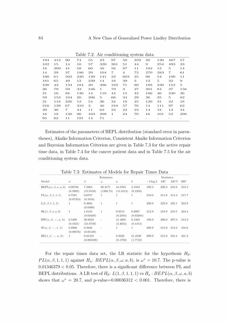
(Proschan [31]). The data is presented in Table 7.2.


Table 7.2: Air conditioning system data194 413 90 74 55 23 97 50 359 50 130 487 57

102 15 14 10 57 320 261 51 44 9 254 493 33

18 209 41 58 60 48 56 87 11 102 12 5 14

14 29 37 186 29 104 7 4 72 270 283 7 61

100 61 502 220 120 141 22 603 35 98 54 100 11

181 65 49 12 239 14 18 39 3 12 5 32 9

438 43 134 184 20 386 182 71 80 188 230 152 5

36 79 59 33 246 1 79 3 27 201 84 27 156

21 16 88 130 14 118 44 15 42 106 46 230 26

59 153 104 20 206 5 66 34 29 26 35 5 82

31 118 326 12 54 36 34 18 25 120 31 22 18

216 139 67 310 3 46 210 57 76 14 111 97 62

39 30 7 44 11 63 23 22 23 14 18 13 34

16 18 130 90 163 208 1 24 70 16 101 52 208

95 62 11 191 14 71 - - - - - - -

Estimates of the parameters of BEPL distribution (standard error in paren-

theses), Akaike Information Criterion, Consistent Akaike Information Criterion

and Bayesian Information Criterion are given in Table 7.3 for the active repair

time data, in Table 7.4 for the cancer patient data and in Table 7.5 for the air

conditioning system data.

Table 7.3: Estimates of Models for Repair Times DataEstimates Statistics

Model α β ω a b −2 logL AIC AICC BIC

BEPL(α, β, ω, a, b) 0.08792 7.5983 69.3171 41.0765 2.1953 199.3 209.3 210.8 218.5

(0.2992) (15.9158) (1260.74) (15.5515) (6.2258)

PL(α, β, 1, 1, 1) 0.7581 0.6757 1 1 1 210.0 214.0 214.3 217.7

(0.07424) (0.1016)

L(1, β, 1, 1, 1) 1 0.4664 1 1 1 220.0 222.0 222.1 223.8

(0.0499)

BL(1, β, 1, a, b) 1 1.6145 1 0.9513 0.2007 212.9 218.9 219.5 224.4

(0.03449) (0.2505) (0.03284)

BW(α, β, −, a, b) 0.5408 36.6023 - 41.4065 0.1263 198.0 206.0 207.0 213.3

(0.1821) (21.0749) (3.4654) (0.1214)

W(α, β, −, 1, 1) 0.8986 0.2949 - 1 1 208.9 212.9 213.2 216.6

(0.09576) (0.05138)

BE(1, β, −, a, b) 1 0.01218 - 0.9322 21.2530 209.9 215.9 216.4 221.3

(0.003109) (0.1793) (1.7710)

For the repair times data set, the LR statistic for the hypothesis H0:

PL(α, β, 1, 1, 1) against Ha: BEPL(α, β, ω, a, b), is ω∗ = 10.7. The p-value is

0.01346379 < 0.05. Therefore, there is a significant difference between PL and

BEPL distributions. A LR test ofH0: L(1, β, 1, 1, 1) vsHa :BEPL(α, β, ω, a, b)

shows that ω∗ = 20.7, and p-value=0.00036312 < 0.001. Therefore, there is


a significant difference between L and BEPL distributions. There is also a

significant difference between PL and L distributions where ω∗ = 10.0 with a

p-value of 0.00107136 < 0.01. Moreover, the values of the statistics AIC and

AICC are smaller for the BEPL distribution and show that the BEPL distri-

bution is a “better” fit than its sub-models for the repair times data, however

a comparison of BEPL and BW distributions shows that the four parameter

BW distribution is slightly better.

The asymptotic covariance matrix of MLEs for BEPL model parameters,

which is the FIM I−1n (Θ), is given by

0.08952 −4.5464 −370.36 4.2174 −1.6999

−4.5464 253.31 19939 −184.68 74.4387

−370.36 19939 1589474 −15981 6439.33

4.2174 −184.68 −15981 241.85 −96.1693

−1.6999 74.4387 6439.33 −96.1693 38.761

and the 95% two-sided asymptotic confidence intervals for α, β, ω, a and b are

given by 0.08792±0.586432, 7.5983±31.194968, 69.3171±2471.0504, 41.0765±30.48094 and 2.1953±12.202568, respectively. Plots of the fitted densities and

the histogram of the repair time data are given in Figure 7.1.


Figure 7.1: Plot of the fitted densities for the Repair Times Data

Table 7.4: Estimates of Models for Cancer Patient DataEstimates Statistics


BEPL(α, β, ω, a, b) 0.9049 0.3352 34.3398 0.0358 0.3598 818.8736 828.8736 829.3659 843.1337

(0.2657) (0.2508) (0.0039) (0.0199) (0.2251)

BPL(α, β, 1, a, b) 0.60245 0.8686 1 2.5744 0.7605 820.8393 828.8393 829.1645 840.2474

(0.2299) (0.4169) - (1.5238) (1.1546)

PL(α, β, 1, 1, 1) 0.8302 0.2943 1 1 1 826.7076 830.7076 830.8636 836.4117

(0.0472) (0.0370)

L(1, β, 1, 1, 1) 1 0.19614 1 1 1 839.0596 841.0596 841.0916 843.9118

(0.0499)

BW(α, β, −, a, b) 0.6689 0.3304 - 2.7257 0.8808 821.3575 829.3575 829.6827 840.7657

(0.2368) (0.4177) (1.5572) (1.3743)

W(α, β, −, 1, 1) 1.0479 0.1046 - 1 1 828.1738 832.1738 832.2698 837.8778

(0.0676) (0.0093)

For the cancer patients data, the LR statistics for the test of the hypotheses

H0 : PL(α, β, 1, 1, 1) against Ha : BEPL(α, β, ω, a, b) and H0 : L(1, β, 1, 1, 1)

against Ha : BEPL(α, β, ω, a, b) are 7.844 (p − value = 0.04956 < 0.05) and


20.186 (p − value = 0.000459 < 0.001), respectively. Consequently, we re-

ject the null hypothesis in favor of the BEPL distribution and conclude that

the BEPL distribution is significantly better than the PL and L distributions.

However, there is no significant difference between the BPL and BEPL distri-

butions based on the LR test. Also, based on the values of the statistics: AIC,

AICC and BIC, we conclude that the BPL distribution is the better fit for the

cancer patient data. The BPL distribution is also slightly better that the BW

distribution based on the values of these statistics. Plots of the fitted densities

and the histogram for the cancer patient data are given in Figure 7.2.

Figure 7.2: Plot of the fitted densities for the Cancer Patients Data


Table 7.5: Estimates of Models for Air Conditioning System DataEstimates Statistics


BEPL(α, β, ω, a, b) 0.7945 0.1509 6.7278 0.2035 0.2303 2064.1 2074.1 2074.4 2090.2

(0.2706) (0.2102) (3.4546) (0.2146) (0.1512)

BPL(α, β, 1, a, b) 0.4316 0.4867 1 3.1251 0.9630 2066.7 2074.7 2074.9 2087.6

(0.0573) (0.1658) (0.4284) (0.8737)

BEL(1, β, ω, a, b) 1 0.0453 7.5488 0.1048 0.2034 2064.8 2072.8 2073.0 2085.8

(0.0194) (3.9156) (0.0623) (0.0649)

BL(1, β, 1, a, b) 1 0.02343 1 0.4842 0.5378 2080.6 2086.6 2086.7 2096.3

(0.00972) (0.0538) (0.2302)

PL(α, β, 1, 1, 1) 0.6609 0.1807 1 1 1 2071.4 2075.4 2075.5 2081.9

(0.0316) (0.0165)

L(1, β, 1, 1, 1) 1 0.0215 1 1 1 2165.3 2167.3 2167.3 2170.5

(0.00111)

BW(α, β, −, a, b) 0.7383 0.2719 - 2.7250 0.1188 2064.6 2072.6 2078.8 2085.6

(0.1114) (0.7861) (4.7308) (0.2421)

W(α, β, −, 1, 1) 0.9109 0.0114 - 1 1 2073.5 2077.5 2077.6 2084.0

(0.0504) (0.00097)

BE(1, β, −, a, b) 1 0.00129 - 0.9048 7.6602 2075.2 2081.2 2081.4 2090.9

(0.000184) (0.0864) (0.3651)

For the air conditioning system data, the LR statistics for the test of the

hypotheses H0 : BL(1, β, 1, a, b) against Ha : BEPL(α, β, ω, a, b) is 16.5 (p −value = 0.000263 < 0.001.) Consequently, we reject the null hypothesis in

favor of the BEPL distribution and conclude that the BEPL distribution is

significantly better than the BL distribution. The LR test statistics for the

test of the hypotheses H0 : BL(1, β, 1, a, b) against Ha : BEL(1, β, ω, a, b)

is 15.8 (p − value = 0.000704 < 0.001), so that the null hypothesis of BL

model is rejected in favor of the alternative hypothesis of BEL model. The

BPL distribution is also significantly better than the PL and BL models based

on the LR test. However, there is no significant difference between the BPL

and BEPL distributions, as well as between the BEL and BEPL distributions

based on the LR test. The sub-models: BPL and BEL are better fits than

the BEPL distribution for the air conditioning system data. Also, the values

of the statistics: AIC, AICC and BIC, points to the BEL distribution, so we

conclude that the BEL distribution is the better fit for the air conditioning

system data. The BEL distribution also compares favorably with the BW

distribution based on the values of these statistics. Plots of the fitted densities

and the histogram for the air conditioning system data are given in Figure 7.3.

Based on the values of these statistics, we conclude that the BEPL distri-

bution and its sub-models can provide good fits for lifetime data. In the first

data set, the BEPL distribution performed better than the BL, PL, L, BE,

and Weibull distributions. The four parameter BW distribution was slightly

better based on the values of AIC, AICC and BIC. In the second data set,


the BPL distribution performed better than the other models including the

beta Weibull distribution. In the third data set, the BEL distribution as well

as the BPL distribution seem to be the better fits, and the BEL distribution

compares favorably with the BW distribution. The BEPL and its sub-models

including the BEL and BPL distributions can provide better fits than other

common lifetime models.

Figure 7.3: Plot of the fitted densities for the Air Conditioning System Data

8 Concluding Remarks

We have developed and presented the mathematical properties of a new

class of distributions called the beta-exponentiated power Lindley (BEPL)

distribution including the hazard and reverse hazard functions, monotonicity

properties, moments, conditional moments, reliability, entropies, mean devia-

tions, Lorenz and Bonferroni curves, distribution of order statistics, and max-


imum likelihood estimates. Applications of the proposed model to real data in

order to demonstrate the usefulness of the distribution are also presented.

ACKNOWLEDGEMENTS.The authors are grateful to the referees for

some useful comments on an earlier version of this manuscript which led to

this improved version.

References

[1] D.V. Lindley, Fiducial distributions and Bayes Theorem, Journal of the

Royal Statistical Society, Series B, 20, (1958), 102 - 07.

[2] M.E. Ghitany, B. Atieh and S. Nadarajah, Lindley Distribution and Its

Applications, Mathematics and Computers in Simulation, 78(4), (2008),

493 - 506.

[3] H. Zakerzadeh and A. Dolati, Generalized Lindley Distribution, Journal

of Mathematical Extension, 3(2), (2009), 13 - 25.

[4] G. Warahena-Liyanage and M. Pararai, A Generalized Power Lindley Dis-

tribution with Applications, Asian Journal of Mathematics and Applica-

tions, 2014(Article ID ama0169), (2014), 1 - 23.

[5] M. Sankaran, The Discrete Poisson-Lindley Distribution, Biometrics,

26(1), (1970), 145 - 149.

[6] A. Asgharzedah, H.S. Bakouch and H. Esmaeli, Pareto Poisson-Lindley

Distribution with Applications, Journal of Applied Statistics, 40(8),

(2013).

[7] S. Nadarajah, H.S. Bakouch and R. Tahmasbi, A Generalized Lindley

Distribution, Sankhya B 73, (2011), 331 - 359.

[8] M.E. Ghitany, D.K. Al-Mutairi, N. Balakrishnan and L.J. Al-Enezi, Power

Lindley distribution and associated inference, Computational Statistics

and Data Analysis, 64, (2013), 20 - 33.


[9] H. Bidram, J. Behboodian and M. Towhidi, The beta Weibull geometric

distribution, Journal of Statistical Computation and Simulation, 83(10),

(2013), 52 - 67.

[10] A. Percontini, B. Blas and G.M. Cordeiro, The beta Weibull Poisson

Distribution, Chilean journal of Statistics, 4(2), (2013), 3 - 26.

[11] N. Eugene, C. Lee and F. Famoye, Beta-normal distribution and its appli-

cations, Communication and Statistics Theory and Methods, 31, (2002),

497 - 512.

[12] M.C. Jones, Families of distributions arising from distributions of order

statistics, Test, 13, (2004), 1 - 43.

[13] S. Nadarajah and S. Kotz, The beta Gumbel distribution, Mathematical

Problems in Engineering 10, (2004), 323 - 332.

[14] S. Nadarajah S and A.K. Gupta, The beta Frechet distribution, Far East

Journal of Theoretical Statistics, 14, (2004), 15 - 24.

[15] S. Nadarajah and S. Kotz, The beta exponential distribution, Reliability

Engineering and System Safety, 91, (2005), 689 - 697.

[16] W. Barreto-Souza, A.A.S. Santos and G.M. Cordeiro, The beta gener-

alized exponential distribution, Journal of Statistical Computation and

Simulation, 80, (2010), 159 - 172.

[17] F. Gusmao, E. Ortega and G.M. Cordeiro, The generalized inverse Weibull

distribution, Statistical Papers, 52, (2011), 591 - 619.

[18] R.R. Pescim, C.G.B. Demetrio, G.M. Cordeiro, E.M.M. Ortega and M.R.

Urbano, The beta generalized half-normal distribution, Computational

Statistics and Data Analysis, 54, (2010), 945 - 957.

[19] K. Cooray and M.M.A. Ananda, A generalization of the half-normal dis-

tribution with applications to lifetime data, Communication and Statistics

Theory and Methods, 37, (2008), 1323 - 1337.

[20] G.M. Cordeiro, C.T. Cristino, E.M. Hashimoto and E.M.M Ortega, The

beta generalized Rayleigh distribution with applications to lifetime data,

Statistical Papers, 54, (2013), 133 - 161.


[21] M. Carrasco, E.M. Ortega and G.M. Cordeiro, A generalized modified

Weibull distribution for lifetime modeling, Computational Statistics and

Data Analysis, 53(2), (2008), 450 - 462.

[22] B.O. Oluyede and T. Yang, A new class of generalized Lindley distribu-

tions with applications, Journal of Statistical Computations and Simula-

tion, (2014), 1 - 29.

[23] E.A. Shannon, A Mathematical Theory of Communication, The Bell Sys-

tem Technical Journal, 27(10), (1948), 379 - 423.

[24] E.A. Shannon, A Mathematical Theory of Communication, The Bell Sys-

tem Technical Journal, 27(10), (1948), 623 - 656.

[25] A. Renyi, On measures of entropy and information, Proceedings of the 4th

Berkeley Symposium on Mathematical Statistics and Probability , Berkeley

(CA):University of California Press, I, (1961), 547 - 561.

[26] C. Lee, F. Famoye and O. Olumolade, Beta-Weibull Distribution: Some

Properties and Applications, Journal of Modern Applied Statistical Meth-

ods, 6, (2007), 173 - 186.

[27] W.H. Alven, Reliability Engineering by ARINC, New Jersey (NJ), Pren-

tice Hall, 1964.

[28] R.S. Chhikara and J.S. Folks, The Inverse Gaussian Distribution as a

Lifetime Model, Technometrics, 19,(1977), 461 - 468.

[29] T. Dimitrakopoulou, K. Adamidis and S. Loukas, A Lifetime Distribution

with an Upside down Bathtub-Shaped Hazard Function, IEEE Transac-

tions on Reliability, 56, (2007), 308 - 311.

[30] E.T. Lee and J. Wang, Statistical Methods for Survival Data Analysis,

New York (NY),Wiley, 2003.

[31] F. Proschan, Theoretical Explanation of Observed Decreasing Failure

Rate, Technometrics, 5, (1963), 375 - 383.

[32] R.M. Corless, G.H. Gonnet, D.E.G. Hare, D.J. Jeffrey and D.E. Knuth,

On the Lambert W function, Advances in Computational Mathematics,

(5), (1996), 329 - 359.


[33] I.S. Gradshteyn and I.M. Ryzhik, Tables of Integrals, Series, and Prod-

ucts, Seventh edition, New York (NY), Academic Press, 2007.

[34] J.P. Klein and M.L. Moeschberger, Survival Analysis: Techniques for Cen-

soring and Truncated Data, Second edition, New York (NY), Springer-

Verlag New York. Inc, 2003.

[35] M. Shaked M and J.G. Shanthikumar, Stochastic Orders and Their Ap-

plications, New York (NY), Academic Press, 1994.


Appendices

R Algorithms

#Define the pdf of BEPL

f1=function(x,alpha,beta,omega,a,b){y=(alpha*beta^2*omega*(1+x âlpha)

*x ^(alpha-1)*exp(-beta*xâlpha) *(1-(1+beta*x âlpha /(1+beta))

*exp(-beta *x âlpha)) ^(omega*a-1)) *(1-(1-(1+beta*x âlpha /(1+beta))

*exp(-beta *x âlpha))ômega) ^(b-1) /(beta(a,b)*(beta+1))

return(y)

}

#Define the cdf of BEPL

F1=function(x,alpha,beta,omega,a,b){

y=pbeta((1-(1+beta*xâlpha/(1+beta))*exp(-beta*xâlpha))ômega,a,b)

return(y)

}

#Define the moments of BEPL

moment=function(alpha,beta,omega,a,b,r){

f=function(x,alpha,beta,omega,a,b,r)

{(x^r)*(f1(x,alpha,beta,omega,a,b))}

y=integrate(f,lower=0,upper=Inf,subdivisions=100

,alpha=alpha,beta=beta,omega=omega,a=a,b=b,r=r)

return(y)

}


#Define the reliability of BEPL

reliability=function(alpha1,beta1,omega1,a1,b1,alpha2,

beta2,omega2,a2,b2){

f=function(x,alpha1,beta1,omega1,a1,b1,alpha2,beta2,omega2,a2,b2)

{f1(x,alpha1,beta1,omega1,a1,b1)*(F1(x,alpha2,beta2,omega2,a2,b2))}

y=integrate(f,lower=0,upper=Inf,subdivisions=100,alpha1=alpha1,

beta1=beta1,omega1=omega1,a1=a1,b1=b1,alpha2=alpha2,

beta2=beta2,omega2=omega2,a2=a2,b2=b2)

return(y)

}

#Define Mean Deviation about the mean of BEPL

delta1=function(alpha,beta,omega,a,b){

mu=moment(alpha,beta,omega,a,b,1)$ value

f=function(x,alpha,beta,omega,a,b){(abs(x-mu)*f1(x.alpha,beta,omega,a,b)}


,alpha=alpha,beta=beta,omega=omega,a=a,b=b)

return(y)

}

#Define Mean Deviation about the median of BEPL

delta2=function(alpha,beta,omega,a,b){

M=median(c(X)) #X is the data set

f=function(x,alpha,beta,omega,a,b){(abs(x-M)*f1(x.alpha,beta,omega,a,b)}


,alpha=alpha,beta=beta,omega=omega,a=a,b=b)

return(y)

}


Define the Renyi entropy of BEPL

t=function(alpha,beta,omega,a,b,gamma){

f=function(x,alpha,beta,omega,a,b,gamma)

{(f1(x,alpha,beta,omega,a,b))^(gamma)}


,alpha=alpha,beta=beta,omega=omega,a=a,b=b,gamma=gamma)$ value

return(y)

}

Renyi=function(alpha,beta,omega,a,b,gamma){

y=log(t(alpha,beta,omega,a,b,gamma))/(1-gamma)

return(y)

}

#Calculate the maximum likelihood estimators and

variance-covariance matrx of the BEPL

library('bbmle');

xvec<-c(X) #X is the data set

fn1<-function(alpha,beta,omega,a,b){

-sum(log(alpha*beta^2*omega/(beta(a,b)*(beta+1)))+log(1+xvecâlpha)

+(alpha-1)*log(xvec)-beta*xvecâlpha+(omega*a-1)

*log(1-(1+beta*xvecâlpha/(beta+1))

*exp(-beta*xvecâlpha))+(b-1)*log(1-(1-(1+beta*xvecâlpha/(beta+1))

*exp(-beta*xvecâlpha))ômega))

} mle.results1<-mle2(fn1,start=list(alpha=alpha,beta=beta,

omega=omega,a=a,b=b),hessian.opt=TRUE)

summary(mle.results1)

vcov(mle.results1)

A New Class of Generalized Power Lindley Distribution with ... 5_1_5.pdf · 54 A New Class of...

Documents

Transcript of A New Class of Generalized Power Lindley Distribution with ... 5_1_5.pdf · 54 A New Class of...