- 1 -

The Generalized Extreme Value (GEV) Distribution,

Implied Tail Index and Option Pricing

Sheri Markose and Amadeo Alentorn

This version: 16 December 2010

Forthcoming Spring 2011 in The Journal of Derivatives

Abstract

Crisis events such as the 1987 stock market crash, the Asian Crisis and the collapse of Lehman

Brothers have radically changed the view that extreme events in financial markets have negligible

probability. This article argues that the use of the Generalized Extreme Value (GEV) distribution to

model the implied Risk Neutral Density (RND) function provides a flexible framework that captures

the negative skewness and excess kurtosis of returns, and also delivers the market implied tail index.

We obtain an original analytical closed form solution for the Harrison and Pliska [1981] no arbitrage

equilibrium price for the European option in the case of GEV asset returns. The GEV based option

pricing model successfully removes the in-sample pricing bias of the Black-Scholes model, and also

shows greater out of sample pricing accuracy, while requiring the estimation of only two parameters.

We explain how the implied tail index is efficacious at modelling the fat tailed behaviour and negative

skewness of the implied RND functions, particularly around crisis events.

- 2 -

The last two decades have been marked by crisis events in financial markets. These include

the 1987 stock market crash, the Asian Crisis (July–October 1997), the September 1998 LTCM

debacle, the bursting of the high technology Dot-Com bubble of 2000-02 with about 30% losses of

equity values, events such as 9/11, sudden corporate collapses of the magnitude of Enron and Lehman

Brothers, and most recently, the 2007/08 credit crisis which has been considered to be the greatest

since the Great Depression. There has been a radical shift in the view held by policy makers, finance

academics and practitioners who now feel that extreme events in financial markets cannot be ignored as

outliers with negligible probability. In mainstream financial theory, extreme events which occur with

small probabilities have not been a matter of concern as in the dominant model of lognormal asset

prices the probability of extreme events such as the stock market crash of October 1987 is virtually

non-existent.1 There has been a growing pragmatic and theoretical shift in interest from the modelling

of ‘normal’ asset market conditions to the shape and fatness of the tails of the distributions of asset

returns which characterize statistical models for extreme events.

Extreme value theory is a robust framework to analyse the tail behaviour of distributions.

Extreme value theory has been applied extensively in hydrology, climatology and also in the insurance

industry. Embrechts et. al. [1997] is a comprehensive source on extreme value theory and applications.

Despite early work by Mandelbrot [1963] on the possibility of fat tails in financial data and evidence

on the inapplicability of the assumption of log normality in option pricing, a systematic study of

extreme value theory for financial modelling and risk management has only begun recently.2

The objective of this article is to use the Generalized Extreme Value (GEV) distribution in the

context of European option pricing with the view to overcoming the problems associated with existing

option pricing models. Within the Harrison and Pliska [1981] asset pricing framework, the risk neutral

probability density (RND) function exists under an assumption of no arbitrage. By definition of a no

arbitrage equilibrium, the current price of an asset is the present discounted value of its expected future

payoff given a risk-free interest rate where the expectation is evaluated by the RND function. Breeden

and Litzenberger [1978] were first to show how the RND function can be extracted from traded option

prices. The Black-Scholes [1973] and lognormal based RND models have well known drawbacks.

First, the implied volatility smiles or smirks are inconsistent with the constancy required in the

lognormal case for volatility across different strikes for options with the same maturity date. Further,

this class of models cannot explicitly account for the negative skewness and the excess kurtosis of asset

returns. Since, Jackwerth and Rubinstein [1996] demonstrated the discontinuity in the implied

skewness and kurtosis across the divide of the 1987 stock market crash - a large literature has

developed which aims to extract the RND function from traded option prices so that the skewness and

fat tail properties of extreme market events are better captured than is the case in lognormal models.

Pricing biases caused by left skewness of asset returns that cannot be captured in the implied

lognormal asset pricing models are now well understood (see,Corrado and Su [1996,1997], Savickas

1 As noted by Jackwerth and Rubinstein [1996] in a lognormal model of assets prices, the market crash on 19 October 1987 with a 29% fall of S&P 500 futures prices has a probability of 10-160, an event which is unlikely to happen even in the life time of the universe. 2 Embrechts et. al. [1999], Mc Neil [1999] and Embrechts [2000] consider the potential and limitations of extreme value theory for risk management. Dowd [2002] gives a good account of these developments and a recent survey of extreme value theory for finance can be found in Rocco [2010].

- 3 -

[2002]). Typically, in periods when the left skewness of asset prices increases, the Black-Scholes

model will overprice out-of-the-money call options and underprice in-the-money call options relative

to when there is greater symmetry in the distribution function. This article shows how the option price

is highly sensitive to changes in the tail shape, which is distinct to its sensitivity to the variance of the

returns distribution. We find that the traded option price implied GEV model for the RND yields results

that strongly challenge traditionally held views on tail behaviour of asset returns based on Gaussian

distributions which predicate simultaneous existence of thin tails in both directions during all market

conditions. The GEV distribution, which is governed by the tail shape parameter, is found to switch tail

shape with underlying market conditions. During extreme market drawdowns, a positive value for the

tail shape parameter results in significant skewness in the probability mass of the GEV density function

for losses and implies extreme price drops with the large probability mass on the right and a truncated

tail in the other direction, implying an upper bound on possible gains. To date, proposed option pricing

models intended to deal with both the fat tail and the skew in asset returns have failed to highlight the

above characteristic features of fat tailed distributions. They have also run into problems ranging from

a lack of closed form solution, a large number of parameters needed or the lack of easy interpretation of

implied parameters. These factors have prevented many of these models from being of practical use in

pricing and hedging options or in risk management for extreme market conditions.

This article argues for the use of the Generalized Extreme Value (GEV) distribution for asset

returns in an option pricing model for the following reasons:

(i) It can provide a closed form solution for the European option price.

(ii) It yields a parsimonious European option pricing model, with only two parameters

to estimate, the tail shape parameter and the scale parameter.

(iii) It provides a flexible framework that subsumes as special cases a number of

classes of distributions that have been assumed to date in more restrictive settings.

The GEV distribution encompasses the three main classes of tail behaviour

associated with the Fréchet type fat tailed distributions and the thin and short

tailed Weibull and Gumbel classes.

(iv) When the GEV distribution is of Fréchet type, it exhibits a fat tail on the right and

a truncated tail on the left. Since extreme economic losses are more probable than

extreme economic gains, we adopt the Fréchet distribution to model extreme

losses. To this end, we follow the practice of the insurance industry, Dowd [2002,

p 272], and model returns as negative returns. As a result, when extreme events

are prominent, the GEV model yields a Fréchet type implied density function for

negative returns, signifying higher probabilities of price drops.

(v) Most significantly, the GEV option pricing model can deliver the market implied

tail index for asset returns. It is important to capture market perception of fat tailed

behaviour in asset returns in a manner which is interspersed with thin and short

tailed Gumbel and Weibull values for the tail index which characterize more

normal market conditions. Hence, the market implied tail index is found to be time

varying in a way that mirrors the lack of invariance in the recursively estimated

- 4 -

tail index of asset returns (see, Quintos, Fan and Phillips [2001]) with jumps in the

fat tailedness in crisis periods.

(vi) We show how the GEV option pricing model removes the well known pricing

biases associated with the Black-Scholes, by capturing the time varying levels of

skewness and kurtosis. We also show how the GEV model yields superior pricing

accuracy out of sample, as GEV implied RNDs are more capable of capturing

extreme market conditions than other option pricing models.

(vii) Having obtained a closed form solution for the option pricing model, we can also

obtain a closed form solution for the new “greek” in the lexicon of option pricing,

which measures the sensitivity of the option price to the tail index.

(viii) The closed form delta hedging formulation can also be given.

This article covers the first six features listed above of the GEV RND model of option pricing

and we leave the last two for further work.

We will now briefly comment on how the GEV RND based option pricing model fits into the

large edifice, given in Exhibit 1 below, built from the different methods used for the extraction of the

implied distributions and their respective option pricing models that have arisen since the work of

Breeden and Litzenberger [1978]. Based on Jackwerth [1999] survey, the different methods can be

classified into three main categories: parametric, semi parametric and non-parametric. Parametric

methods can be divided into three sub-categories: generalized distribution methods, specific

distributions and mixture methods. Generalized distribution methods introduce more flexible

distributions with additional parameters beyond the two parameters of the normal or lognormal

distributions. Within this subcategory, Aparicio and Hodges [1998] use generalized Beta functions of

the second kind, which are described by four parameters, and Corrado [2001] uses the generalized

Lambda distribution. Under the specific distributions being assumed for the RND function, the Weibull

distribution is used by Savickas [2002], and the skewed Student-t by de Jong and Huisman [2000]. The

Variance Gamma distribution used by Madan, Carr and Chang [1998], and Levy processes used among

others by Matache, Nitsche and Schwab [2004] are more recent specifications with these methods

having parameters that can control fat tails and skewness of the asset price. Up to seven parameters are

associated with these models.

Finally, the third sub-category within parametric methods is the mixture methods, which

achieve greater flexibility by taking a weighted sum of simple distributions. The most popular method

here is mixture of lognormals. Ritchey [1990] and Gemmill and Saflekos [2000] use two lognormals,

and Melick and Thomas [1997] use three lognormals. One problem associated with the mixture of

distributions is that the number of parameters is usually large, and thus they may overfit the data. For

example, the mixture of two lognormals needs to estimate five parameters.

Under the category of semi parametric methods, the Hypergeometric function was used by

Abadir and Rockinger [1997], and expansion methods such as the Gram-Charlier and Edgeworth

expansions, respectively, were used by Corrado and Su [1996] and Corrado and Su [1997]. The non-

parametric methods can be divided again into three groups: kernel methods, maximum-entropy

methods, and curve fitting methods. Kernel methods, implemented in Ait-Sahalia and Lo [1998], are

- 5 -

related to regressions since they try to fit a function to observed data, without specifying a parametric

form. Second, the methods based on maximum-entropy used by Buchen and Kelly [1996] find a non-

parametric probability distribution that tries to match the information content, while at the same time

satisfying certain constraints, such as pricing observed options correctly. In the third group in this

category, there are the curve fitting methods that try to fit the implied volatilities with some flexible

function. The most popular of these is Shimko [1993] who introduced the concept of smoothed implied

volatility smiles which involved fitting typically a cubic or low order polynomial spline to obtain the

middle portion of the RND function. The tails of the RND function were modelled as log normal. This

approach was improved by Bliss and Panigirtzoglou [2002] with the use of a “smoothing spline” whilst

retaining log normal tails. Figlewski [2010] made an advance on this by appending tails from the GEV

distribution which are able to reflect extreme market conditions.

Exhibit 1 Classification of most common RND estimation methods

Parametricmethods

Non-parametricmethods

Generalizeddistributions

Specificdistributions

Mixturemethods

Generalized Beta functions (Aparicio and Hodges [1998])

Generalized Lambda Distribution (Corrado [2001])

Generalized Extreme Value (GEV) distribution

Mixture of two lognormals (Ritchey [1990])

Mixture of three lognormals (Melick and Thomas [1997])

Kernel methods (Aït-Sahalia and Lo [1998])

Maximum entropy methods (Buchen and Kelly [1996])

Curve fitting methods (Shimko [1993], Figlewski [2010])

Semi parametricmethods

Hypergeometric functions (Abadir and Rockinger [1997])

Gram-Charlier expansions (Corrado and Su [1996])

Edgeworth expansions (Corrado and Su [1997])

Weibull distribution (Savickas [2002])

Skewed Student-t (de Jong and Huisman [2000])

Variance Gamma (Madan et al [1998])Lévy process (Matache et al [2004])

- 6 -

The model presented in this article, as highlighted in Exhibit 1, falls in the general category of

parametric models, and more specifically, within the sub-category of generalized distributions. In order

to estimate tail behaviour at high confidence levels, such as 99%, many non-parametric methods for

RND estimation fail to capture tail behaviour of the distributions because of sparse data for options

traded at very high or very low strikes prices. Hence, parametric models have become unavoidable.

This, however, replaces sampling error with model error. In the next section, we give a brief

introduction to Extreme Value Theory and present the Generalized Extreme Value (GEV) distribution

and its properties to indicate how the flexibility of this three parameter class of distributions can

capture skew and fat tails as and when dictated by the data with no a priori restrictions on the class of

distribution. This data driven selection of the tail index mitigates model error.

The rest of the article is organized as follows. We develop the GEV option pricing model and

the closed form solutions for the arbitrage free European call and put option prices are derived for the

GEV based RND function. We then proceed to discuss the components of the closed form solution and

their theoretical properties in terms of moneyness and then tail shape parameter. The empirical section

reports on the results for the estimated implied GEV RND function and for its parameters based on the

FTSE 100 European option price data from 1997 to 2009. The in sample fit of the postulated GEV

option pricing model is compared with the benchmark Black-Scholes one and is found to be superior at

all levels of moneyness and at all time horizons, removing the well known price bias of the Black-

Scholes model. Out of sample pricing tests show that the GEV provides superior pricing performance

compared to Black-Scholes, for one day ahead forecasts. The analysis of the time series characteristics

of the implied tail index is given and the role of implied RND functions in event studies surrounding

periods of “extreme” price falls of the FTSE-100 index is also discussed. Finally, we make concluding

remarks and discuss future work.

EXTREME VALUE THEORY AND THE GEV DISTRIBUTION

Unlike the normal distribution that arises from the use of the central limit theorem on sample

averages, the extreme value distribution arises from the limit theorem of Fisher and Tippet [1928] on

extreme values or maxima in sample data. The class of GEV distributions is very flexible with the tail

shape parameter ξ (and hence the tail index defined as α= ξ-1) controlling the shape and size of the tails

of the three different families of distributions subsumed under it. These three families of distributions

can be nested into a single parametric representation, as shown by Jenkinson [1955] and von Mises

[1936]. This representation is known as the “Generalized Extreme Value” (GEV) distribution and is

given by:

( )( )ξξ ξ /11exp)( −+−= xxF with 0,01 ≠>+ ξξ x (1.a)

Applying the formula that xex −− →+ ξξ /1)1( , as 0→ξ we have:

)exp()(0xexF −−= (1.b)

- 7 -

The standardized GEV distribution, in the form in von Mises [1936] (see, Reiss and Thomas [2001], p.

16-17), incorporates a location parameter µ and a scale parameter σ , in addition to the tail shape

parameter, ξ, and is given by:

( )

−+−=− ξ

σµξ σµξ

/1

,, 1exp)(x

xF with ( )

001 ≠>−+ ξσ

µξ x (2.a)

and

( ))exp()(,,0

σµ

σµ

−−−=

x

exF with 0=ξ (2.b)

The corresponding probability density functions obtained by taking the derivative of the distribution

functions, are respectively:

( ) ( )

−+−

−+=−−− ξξ

σµξ σµξ

σµξ

σ

/1/11

,, 1exp11

)(xx

xf 0≠ξ (3.a)

and

)(exp1

)( /)(/)(,,0

σµσµσµ σ

−−−− −= xx eexf 0=ξ (3.b)

We will now discuss how the tail shape parameter, ξ, determines both the higher moments of

the density function and also the skew in the probability mass leading to truncation points in the

distribution. The tail shape parameter ξ=0 yields thin tailed distributions with the tail index α= ξ-1

being equal to infinity, implying that all moments of the distribution are either finite or zero. 3 When ξ

= 0, the GEV distribution belongs to the Gumbel class and includes the normal, exponential, gamma

and lognormal distributions, where only the lognormal distribution has a moderately heavy tail. The

Gumbel class has zero skew in the probability mass and displays symmetry in the right and left tails.

Further, as seen in equation (2.b) there are no conditions truncating the distribution in either direction

for values of x. The distributions associated with ξ > 0 are called Fréchet and these include well known

fat tailed distributions such as the Pareto, Cauchy and Student-t distributions. Finally, in the case where

ξ < 0, the distribution class is Weibull.4 These are short tailed distributions with finite upper bounds

and include distributions such as uniform and beta distributions. In distributions for which ξ ≠ 0, the

equality condition in equation (2.a) imposes a truncation of the probability mass and a distinct

asymmetry in the right and left tails such that when the probability mass is high at one tail signifying

non-negligible probability of an extreme event in that direction, there is an absolute maxima (or

minima) in the other direction beyond which values of x have zero probability. As shown in Reiss and

Thomas [2001], kurtosis of the Fréchet distribution becomes infinite at ξ ≥ 0.25 (the tail index, α ≤ 4),

and all higher moments including kurtosis and the right skew become infinite at ξ ≥ 0.33 (the tail

index, α ≤ 3). Even for small positive values of ξ, approximately at about ξ = 0.1, the rate of growth of 3 The general rule is that the nth and higher moments fail to be finitely integrable if the tail index is smaller than n. When ξ ≤ 0, all moments are finite or zero. However, when ξ≥ 0, only moments up to the integer part of the tail index, α =1/ ξ, exist with all other moments being infinite. 4 Here we make reference to the Weibull distribution as defined in the context of extreme value theory, Embrechts [1997, p154].

- 8 -

skewness and kurtosis of the distribution, with both fast approaching infinite growth, results in a

concentration of the probability density of the Fréchet distribution at the right tail. Thus, as ξ increases

with ξ > 0, the truncation points at the left tail at which there is zero probability become more stringent.

Note for ξ < 0, for the Weibull class of distributions, there is increased probability mass on the left tail

and a truncation point given by the inequality in equation (2.a) at the right tail. However, it is well

known (see, Reiss and Thomas [2001]) that at about ξ = -0.3, the Weibull distribution has zero skew

and is indistinguishable from a Gumbel distribution.

As the probability of extreme economic losses are more likely than extreme gains, economic

losses are modelled as a Fréchet distribution with high probability mass on the right tail. Exhibit 2a

below illustrates the GEV density functions for negative asset returns for each of the three classes of

distributions that the GEV can take based on the shape parameter ξ. Note, that the three graphs only

differ in the value of ξ (the values considered for ξ are 0.3, 0, -0.3), having the same value for location

(µ=0) and scale (σ=0.2) parameters. The initial stock price is assumed to be 100. The corresponding

density functions for the price in each of the three cases for the tail shape parameter are shown in

Exhibit 3. Note, the left skew in the price density function is greatest in Exhibit 3c, for the case when ξ

> 0, and the negative returns density function belongs to the GEV-Fréchet class. Given the value being

assumed, ξ = 0.3, in Exhibits 2c and 3c, as noted above, there is infinite kurtosis and a very stringent

truncation on positive returns exceeding 0.667 or for the prices to rise above 166.67.5 Likewise, for

ξ = - 0.3 in (2.a,3.a), we have zero probability for negative returns to be greater than 0.667 and the

price to fall below 33.33. These upper and lower bounds on returns and prices implied by the GEV

distribution play an important role in the analysis that follows. As will be shown later, for the range of

values for the implied tail shape parameters for 30 day returns on the FTSE-100 index that we extract

on a daily basis from option prices over the sample period from 1997-2009, the maximum value we

obtain for ξ is +0.12. As this implies a tail index value of α = 8.33, it is clear that this guarantees finite

skewness and kurtosis for the risk neutral density function for the entire sample period. Further, on

using equation (2.a), precise truncations values under the RND Q- measure can be determined for the

levels of the stock index and for the returns on it. In the context of the option pricing model it is

important to verify that the truncated values implied by a GEV based RND, ie. Q-impossible events are

also not P-possible in terms of the empirically realized values for prices and returns.6 This will be

investigated in the next section.

Exhibit 2 Density functions for negative returns

5 By rearranging the inequality in equation (2.a) and using the values being assumed for the GEV parameters, the truncation values denoted by x* for negative returns in Exhibits (2.c, 3.c)) and (2.a,3.a) are determined from x*> µ− σ/ ξ. 6 We are grateful to Stephen Figlewski for bringing this to our attention.

- 9 -

(a) ξ = - 0.3

(b) ξ = 0

(c) ξ = + 0.3

Notes: Density function of negative returns as modeled by the (a)GEV-Weibull, (b)GEV-Gumbel and

(c)GEV-Fréchet.

Exhibit 3 Density functions for prices

(a) ξ = - 0.3

(b) ξ = 0

(c) ξ = + 0.3

Notes: Corresponding density function for prices where negative returns have been modeled as (a)

GEV- Weibull, (b) GEV- Gumbel and (c) GEV- Fréchet.

THE GEV OPTION PRICING MODEL Arbitrage Free Option Pricing and the Risk Neutral Density

Let St denote the underlying asset price at time t. The European call option with price Ct is

written on this asset with strike K and maturity T. We assume the interest rate r is constant. Following

the Harrison and Pliska [1981] result on the arbitrage free European call option price, there exists a risk

neutral density (RND) function, g(ST), such that the equilibrium call option price can be written as:

( ) [ ] ( )∫∞−−−− −=−=

K TTTtTr

TQt

tTrt dSSgKSeKSEeKC )()0,max( )()( (4)

Here, Q is the risk neutral measure and [ ]⋅Q

tE is the risk-neutral expectation operator conditional on

information available at time t, g(ST) is the risk-neutral density function of the underlying at maturity.

Similarly, the arbitrage free option pricing equation for a put option is given by:

[ ] ∫ −=−= −−−− K

TTTtTr

TQt

tTrt dSSgSKeSKEeKP

0

)()( )()()0,max()( (5)

In an arbitrage-free economy, the following martingale condition must also be satisfied:

( )T

Qt

tTrt SEeS )( −−= (6)

European Call and Put Option Price with GEV returns

- 10 -

We assume that the RND function g(ST) in (4) for a holding period equal to time to maturity of

the option is represented by the GEV distribution. We derive closed form solutions for the call and put

option pricing equations by analytically solving the integrals in (4) and (5). For the purpose of

obtaining an analytic closed form solution, it was found necessary to define returns as simple returns.7

We define simple negative returns as follows:

t

T

t

tTTT S

S

S

SSRL −=−−=−= 1 (7)

In keeping with the extreme value distribution modelling of economic losses, LT is assumed to follow

the GEV distribution given in (3.a), 0≠ξ ,and hence the density function for the negative returns is

given by:

( ) ( )

−+−

−+=−−− ξξ

σµξ

σµξ

σ

/1/11

1exp11

)( TTT

LLLf (8)

Note, the relationship between the density function for LT in (8) and the RND function g(ST) in (4) for

the underlying price ST is given by the general formula:

( ) ( ) ( )t

TT

TTT S

LfS

LLfSg

1=∂∂= (9)

On substituting (8) into (9), we obtain the RND function of the underlying price in terms of the GEV

density function as in equation (3.a) :

( ) ( )

−+−

−+=−−− ξξ

σµξ

σµξ

σ

/1/11

1exp11

)( TT

tT

LL

SSg (10)

with

( ) 0111 >

−−+=−+ µ

σξµ

σξ

t

TT S

SL (11)

We will first consider the case when ξ>0 and 0 <ξ < 1.8 As already discussed, in this case the

negative returns distribution is Fréchet and this implies that the price RND function g(ST) in (10), in

order to satisfy the condition in (11), is truncated on the right. Hence, the upper limit of integration for

7 Note, simple returns can give rise to the theoretical possibility of negative stock prices when ξ > 0. However, for purposes of option pricing this does not pose a problem as for the call price the lower limit of integration K for the stock price in equation (4) is always positive and likewise for the put price the lower limit of integration for the stock price in equation (5) is zero. Additionally, numerical results (not reported in this article) show that the implied GEV parameters (ξ, σ) obtained when using simple returns are not statistically different to the ones obtained using log returns. 8 The condition 0< ξ <1 is necessary to rule out the case that the first moment for the stock price at maturity is infinite and the option value becomes infinite. In this article all cases of ξ>0 will be constrained in this way. The closed form solution for the call option for the case when 0< ξ <1 is identical to the one obtained for the case when ξ < 0. This is also true for the closed form solution for put option prices. Appendix B derives the closed form solutions for the call and the put options in the case of ξ = 0.

- 11 -

the call option price in (4) becomes ( )ξσµ +−1tS .9 Substituting g(ST) in (10) into the call price

equation in (4), we have:

( ) ( ) ( ) ( )( )∫

+−−−−

−−

−+−

−+−=ξσµ

ξξ

σµξ

σµξ

σ1

/1/11)( 1exp1

1tS

K TTT

tT

tTrt dS

LL

SKSeKC (12)

Consider the change of variable:

( )

−−+=−+= µ

σξµ

σξ

t

TT S

SLy 111 (13)

Under this change of variable, the underlying price ST and dST can be written in terms of y as follows:

( )

−−−= 11 ySS tT ξσµ and dySdS tT ξ

σ−= (14)

Also, the density function in (10) for the underlying price at maturity in terms of y becomes:

( ) ( )ξξ

σ/1/11 exp

1)( −−− −= yy

Syg

t

(15)

Note that under the change of variable the lower limit of integration for the call option equation in (12)

becomes:

−−+= µ

σξ

tS

KH 11 (16)

The upper limit of integration in (12) becomes 0. Substituting for ST and dST as defined in (14) into

(12), and using the new limits of integration we have:

( ) ( ) ( ) dySyyS

KySeC tt

H ttTr

t

−−

−

−−−= −−−−∫ ξ

σσξ

σµ ξξ /1/110)( exp1

11 (17)

Simplifying and rearranging (17) we have:

9 On the other hand, when ξ < 0 the GEV density function for ST is truncated on the left, and therefore, the lower limit of integration for the call option price in (4) becomes max[K, St (1 - µ + σ/ξ)] and the upper limit remains ∞. However, the closed form solutions for the call option are identical for both cases when ξ > 0 and ξ < 0. This also holds for put option prices.

- 12 -

( ) ( ) ( )

( ) ( ) ( ) ( )

−

+−−=

−

−

+−−−=

−

−

−−−−=

∫∫

∫

−−−−−−

−−−−

21

0 /1/110 /1/11

/1/110)(

11

exp1exp1

exp111

ψξσµψ

ξσ

ξ

ξσµ

ξσ

ξ

ξσµ

ξ

ξξξξ

ξξ

KSS

dyyyKSdyyyyS

dyyyKySeC

tt

HtH

t

H ttTr

t

(18)

The integral 1ψ in (18) above can be solved by applying the change of variable ξ/1−= yt , and then it

can be evaluated in terms of the incomplete Gamma function, yielding the following solution:

( ) ( )ξξξ ξξψ /10 /1/11 ,1exp −−− −Γ−=−= ∫ Hdyyy

H (19)

The solution of integral 2ψ in (18) is:

( ) ( ) ( )[ ] ( )( )ξξξξ ξξψ /10/10 /1/112 expexpexp −−−−− −−=−=−= ∫ Hydyyy HH

(20)

Combining results for 1ψ and 2ψ , we obtain a closed form for the GEV call option price:

( ) ( )

−

−

+−−−Γ−=−−−−− ξ

ξσµξ

ξσ ξ /1

1,1)( /1)( Ht

ttTrt eKSH

SeKC (21)

Grouping the terms with St together we have:

( ) ( )

−

−Γ−+−=−− −−−−− ξξ ξξ

ξσξσµ

/1/1 /1)( ,11)( HHt

tTrt eKHeSeKC (22)

Theoretically, the application of the Girsanov Theorem (see, Neftci [2000]) to option pricing

implies that the empirical distribution and the risk neutral distribution need to have the same support.

By the Girsanov Theorem, the price levels and the size of returns that are Q-impossible due to the

application of the truncation condition in (11) should not be P-possible, and vice versa, in terms of the

realized historical prices and returns. We find that the conditions of the Girsanov Theorem are satisfied

for the sample period for which the implied GEV based RND is extracted from option prices. The

analysis of this is given in Appendix D.

Following similar steps, we can also derive a closed form solution for the put option price under

GEV returns.10 Details of this derivation can be found in the Appendix A, which yields the following

equation:

10 Once the call pricing formula is derived, one could simply obtain the put pricing formula using the put-call parity relationship. We numerically verified that the independently derived call and put pricing formulas satisfy put-call parity.

- 13 -

( ) ( )( ) ( )

−Γ−−+−−−= −−−−−−−− −−−− ξξξ

ξσξσµ

ξξξξ /1/1)( ,,11)(/1/1/1/1

HheeSeeKeKP hHt

HhtTrt

(23)

where ( ) 011 >−+= µσξh . Note that h is a constant, given a set of parameters µ, σ, and ξ.

In the following sections, we will analyse the properties of the GEV RND based closed form solutions

for the call and put options under different moneyness conditions and values for the tail shape

parameter.

Analysis of the GEV call option pricing model

This section aims to give some insights into the closed form solution for the GEV based call

option pricing equation given in (22), which has two components and respective probability weights

involving St and K. These two components can be interpreted along the same lines as the Black-Scholes

model. The key to understanding the GEV option pricing formula lies with the term,

ξ

ξµ

σξ

/1

/111

−

−

−−+−

− = tS

K

H ee (24)

This term is the cumulative GEV distribution function as defined in (2.a) for the “standardized

moneyness” of the option defined as (St – K)/St. Hence, it corresponds to the risk neutral probability p

of the call option being in the money at maturity.11 For a given set of implied GEV parameters

{ µ, σ , ξ} we can work out (see, Exhibit 4) the range of exercise prices K in relation to the given St

which yield: ξ/1−−He = 1 for deep in-the-money call options,

ξ/1−−He = 0 for deep out-of-the-money

call options, and 0 < ξ/1−−He < 1 for all other cases.

Exhibit 4 below plots the probability p= ξ/1−−He of exercising the option at maturity, given by

the GEV model with two different values of ξ, and also for the Black-Scholes model. 12 When ξ>0, the

density function of losses is Fréchet, and thus, the implied price density function is left skewed with a

fat tail on the left, as shown respectively in Exhibits 2c and 3c. Since the latter implies there is a higher

probability of downward moves of the underlying than in the Black-Scholes case, we see from Exhibit

4 how the probability of exercising the call option when ξ > 0 approaches 1 much slower than for the

Black-Scholes model.

Exhibit 4 Probability of the call option being in the money at maturity

11 Recall that in the case of the Black-Scholes model the probability of the option being in the money at maturity is given by

N(d2), where N() is the standard cumulative normal distribution function, and TTrKSd t σσ /])2/()/[ln( 22 −+=

12 To make the three cases comparable, we use the same traded call option price data to estimate the GEV model and the Black-Scholes model. Then, to obtain the second case for the GEV model, we fix ξ to be equal to the initial estimate, but with opposite sign, and estimate the other two GEV parameters.

- 14 -

Notes: The probability of the call option being in the money at maturity is given by pGEV=exp(-H-1/ ξ)

for the GEV case, and by pB-S=N(d2) for the Black-Scholes. The positive and negative values of ξ used

for the GEV distribution are 0.16 and -0.16 respectively.

On the other hand, when ξ < 0, the GEV density of the losses is of Weibull type, and thus the

implied price density function is right-skewed, resulting in a higher probability of upward moves.

Therefore, the probability p of exercising the option as we lower the strike price K reaches 1 faster than

in the Black-Scholes case. Note that for high strike prices and for any value of ξ ≠ 0, the probability of

the option being in the money goes to zero faster than for the Black-Scholes case.

When the call option is deep in-the-money (ITM) with K << St and ξ/1−−He = 1 , the call

price converges to a linear function of the expected payoff (see Appendix C for proof). Thus,

[ ]( ) KeSKSEeKC tTrtT

QGEVt

tTrt

)()()( −−−− −=−= (25)

Here [ ]TQGEVt SE is the conditional first moment of the price RND function, which by the

martingale condition in (6) equals St. For this range of strike prices, the option prices obtained with the

GEV model converge to those given by the Black-Scholes model. When the option is deep out of the

money, then K >> St and ξ/1−−He = 0, and it is easy to verify that the call price is zero.

Exhibit 5 displays the call option prices obtained from the GEV model and the Black-Scholes

model. The Black-Scholes model overprices the out-of-the-money (OTM) call options relative to the

GEV model in both cases. In the OTM case, the GEV model yields higher values of call prices when

ξ< 0 than when ξ > 0. This is because when ξ< 0, upward movements in the underlying price are more

likely and the price density is truncated on the left (see Exhibit 3a). On the other hand, when ξ > 0

downward movements in the price are more likely and the price density function is truncated on the

right (see Exhibit 3c). Hence, in the OTM region of high exercise prices, K, the GEV price with ξ > 0

gives the lowest prices for the call option.

- 15 -

Exhibit 5 Call option prices for the GEV model and the Black-Scholes model

Notes: The positive and negative values of ξ used for the GEV distribution are 0.16 and -0.16

respectively.

For in-the-money (ITM) options, as seen in Exhibit 5, the Black-Scholes model under prices

call options when compared to the GEV model, and the GEV model gives higher option prices when ξ

> 0 than when ξ < 0. This can be explained in terms of the asymmetry in the peakedness of the two

densities. When ξ > 0, the RND function for the price is left skewed, with peakedness at higher values

of the underlying than when ξ < 0. For at-the-money (ATM) options, the prices given by both models

are approximately the same. Note that for deep ITM options, i.e. for much lower values of K (not

shown in the graph) both GEV and Black-Scholes prices converge to the present discounted value of

the intrinsic value of the option, increasing linearly as K falls.

Analysis of the GEV put option pricing model

The analysis for the closed form solution of the GEV put option pricing model in equation

(23) is analogous to what was done in the case of the call option. The probability of a put being in the

money is given by

ξξξ /1/1/1

1−−− −−− −≈− HHh eee (26)

Here, note ξ/1−−he is approximately equal to 1 and hence (26) is one minus the probability of

the call being in the money at maturity. In Exhibit 6, while considering the case of a Fréchet

distribution for losses with ξ > 0, for low strike prices relative to the underlying, we have a greater

probability of the put option being in the money at maturity as compared to either the Black-Scholes

case or the GEV case when ξ < 0.

Exhibit 6 Probability of the put option being in the money at maturity

- 16 -

Notes: the probability of being in the money for the put option at maturity is given by pGEV=1 - exp(-H-

1/ ξ) for the GEV case, and by pB-S=N(-d2) for the Black-Scholes. The positive and negative values of ξ

used for the GEV distribution are 0.16 and -0.16 respectively.

Exhibit 7 below displays the put option prices obtained with the GEV model along with the

Black-Scholes model. The Black-Scholes model substantially underprices the out-of-the-money (OTM)

put options relative to the GEV model. The GEV model yields higher values of OTM put prices when ξ

> 0 than when ξ < 0. For in-the-money (ITM) put options, the Black-Scholes model only marginally

overprices put options with respect to the GEV model. The GEV model gives higher prices for ITM put

options when ξ < 0 than when ξ > 0. For at-the-money (ATM) options, the prices given by both the

GEV and the Black-Scholes models are approximately the same. Note that for deep ITM put options,

both GEV and Black-Scholes prices converge to the present discounted value of the intrinsic value of

the option, ttTr SKe −−− )( , which increases linearly with K.

Exhibit 7 Put option prices for the GEV model and the Black-Scholes model

Notes: The positive and negative values of ξ used in the case of the GEV model are 0.16 and -0.16

respectively.

- 17 -

RESULTS Data description

The data used in this study are the daily settlement prices of the FTSE 100 index call and put

options published by the London International Financial Futures and Options Exchange (LIFFE). These

settlement prices are based on quotes and transactions during the day and are used to mark options and

futures positions to market. Options are listed at expiry dates for the nearest four months and for the

nearest June and December. FTSE 100 options expire on the third Friday of the expiry month. The

FTSE 100 option strikes are in intervals of 50 or 100 points depending on time-to-expiry, and the

minimum tick size is 0.5. There are four FTSE 100 futures contracts a year, expiring on the third Friday

of March, June, September and December.

The LIFFE exchange quotes settlement prices for a wide range of options, even though some

of them may have not been traded on a given day. In this study we only consider prices of traded

options, that is, options that have a non-zero traded volume on a given day. The data was also filtered

to exclude days when the cross-section of options had less than three option strikes. Also, options

whose prices were quoted as zero, had less than one week to expiry, or more than 120 days to expiry

were eliminated. Finally, option prices were checked for violations of the monotonicity condition.13

The period of study is from 2-Jan-1997 to 1-Jun-2009. Exhibit 8 below summarizes the

average number of traded option prices available on a daily basis, across both strikes and maturities, for

each of the years in the period under study, including both call and put options. We can see how the

number of traded contracts has increased substantially through time, from an average of 45 daily traded

option prices in 1997 to 159 such prices in 2009. The range of strikes with options traded has also

widened through time.

Exhibit 8 Summary data on FTSE-100 Index option prices

Period Number of option prices

(daily average) Minimum strike Maximum strike

1997 45 3125 5625 1998 61 3625 6825 1999 82 4025 7625 2000 98 4025 9125 2001 127 3775 7125 2002 126 2125 6725 2003 118 2425 5825 2004 124 2625 5825 2005 112 2325 5825 2006 114 2525 6625 2007 144 4025 7725

13 Monotonicity requires that the call (put) prices are strictly decreasing (increasing) with respect to the exercise price. A small number of option prices that did not satisfy this condition were removed from the sample.

- 18 -

2008 164 3625 9025 2009 159 2600 9025 All Years 113 2125 9125

Notes: Average number of traded option prices available per day, minimum and maximum strike price

with options trade per year (Jan 1997-June2009).

The European-style FTSE100 options, though they are options on the FTSE 100 index, can be

considered as options on FTSE-100 index futures, because the futures contract expires on the same date

as the option. Therefore, the futures will have the same value as the index at maturity, and can be used

as a proxy of the underlying FTSE 100 index. By using this method, we avoid having to use the

dividend yield of the FTSE 100 index, and the martingale condition in (6) becomes:

( )TQtt SEF = (27)

Here Ft is the price of the FTSE 100 futures contract at t, and ST is the FTSE 100 index at

maturity T. This martingale condition can be used to reduce the number of parameters in the GEV

model from 3 to 2. This is analogous to the procedure in the Black-Scholes model where the mean of

the distribution is obtained from the martingale condition and only the volatility parameter needs to be

estimated. In the GEV case, the mean of the distribution does not directly correspond to the location

parameter. Instead, the mean of the GEV distribution, as shown in Reiss and Thomas [2001], is a

function of all three parameters and is defined as σξξµ )/)1)1(( −−Γ+ . We can use this definition of the

GEV mean together with (6) to express the location parameter µ in terms of the futures price TtF , ,

current spot price, and the GEV scale and tail shape parameters σ and ξ:

( ) σξξµ

−−Γ−−= 111 ,

t

Tt

S

F (28)

The risk-free rates used are the British Bankers Association’s 11 a.m. fixings of the 3-month

Short Sterling London InterBank Offer Rate (LIBOR) obtained from the website www.bba.org.uk.

Even though the 3-month LIBOR market does not provide a maturity-matched interest rate, it has the

advantages of liquidity and of approximating the actual market borrowing and lending rates faced by

option market participants (Bliss and Panigirtzoglou [2004]).

The option data used in this study can be divided into 6 moneyness categories given in

Figlewski [2002].14 Exhibit 9 below reports the number of observations for call and put options in each

category of moneyness and maturity.

Exhibit 9 Number of observations in each maturity and moneyness category 14 Figlewski [2002] explains that a measure of option moneyness should include an adjustment for volatility and maturity. Following his definition, we calculate the moneyness of an option as )/()/ln( TKeS BSrT

t σ− , where BSσ is the Black-

Scholes implied volatility for each option.

- 19 -

Number of Observations

Subsample Calls Puts

Maturity < 30 days 25,710 31,672 30 to 60 days 24,553 31,534 60 to 90 days 15,463 19,597 90 to 120 days 8,159 9,905

Moneyness deep OTM 8,421 17,895 OTM 23,507 38,043 ATM 30,086 26,808 ITM 8,171 5,790 deep ITM 3,701 4,172

Total 73,885 92,708 Notes: Number of observations of traded options for different maturity and moneyness categories

(January 1997- June 2009).

Here, moneyness for a given option indicates how many standard deviations, σ, the strike

price is away from the current underlying price in terms of the volatility, maturity of the option. An

option is deep out-of-the-money (Deep OTM) if it is more than 1.5 σ out of the money, and similarly, it

is deep in-the-money (Deep ITM) if it is more than 1.5 σ in-the-money. An option is classified as being

at the money (ATM) if it is 0.5 σ in either direction of OTM and ITM. An additional classification is

done for maturity, in terms of days to expiration. Note that there are options data available for time to

expiration longer than 120 days, but the number of prices available for such long time horizons is small

and the options are traded less frequently.

As can be seen in Exhibit 9, the short to medium term time to maturity, the first two groups,

have the greatest number of data points, for both puts and calls. In terms of moneyness, the largest

number of observations is found in the OTM and ATM category, while the deep ITM has the least

number of observations for both puts and calls (ITM options are typically very expensive, as the option

premium includes the intrinsic value, and thus are not traded often).

Empirical Methodology

For each quarterly expiration date in our data period, a total of 49 from March 1997 to March

2009, a target observation date was determined with horizons of 90, 60, 30 and 10 days to maturity. If

no options were traded on the target observation date, the nearest date with traded options was used.

All traded option prices available for each target observation date were used, subject to the filters

discussed above, across all strikes and across all maturities, giving a one year constant horizon implied

RND.15 The implied RND was derived using the GEV and the Black-Scholes option pricing models.

15 In order to estimate a single scale parameter to fit the prices of options across multiple horizons, we need to annualise the scale parameter σ in the pricing equations. This is similar to the procedure used in the Black-Scholes model such that the implied volatility parameter represents an annualised value. To achieve this, at the estimation stage, we replace the GEV scale parameter sigmaσ by Tσ , where T is the time to maturity of the option, in number of years.

- 20 -

For each of these target observation dates a single implied RND was fitted using both put and call

prices.

The GEV model was estimated by minimizing the sum of squared errors (SSE) between the

option prices D~

given by the analytical solution of the GEV option pricing equations in (22) and (23)

and the observed traded option prices D (including both calls and puts) with strikes Ki, as indicated

below:

( )

−= ∑

=

N

iitit KDKDtSSE

1

2

,)(

~)(min)(

σζ (29)

Note that for the GEV model, we minimise the sum of squared errors with respect to only two

GEV parameters, ie. scale and tail shape parameters, σ and ξ. We use equation (28) to substitute out

the location parameter µ which has been derived as function of the futures price, TtF , , current spot

price, and these two parameters. For the Black-Scholes model, we likewise derive a single implied

volatility parameter using both call and put prices. The optimization was performed using the non-

linear least squares algorithm from the Optimization toolbox in MatLab.

In sample pricing performance

The in sample pricing performance tests consist of estimating the implied densities at time t,

by using option prices at time t as well, and then analysing how well the model fits the same option

prices. The pricing performance is reported in terms of the root mean square error RMSE, which

represents the average pricing error in pence per option:

N

tSSEtRMSE

)()( = (30)

For each maturity horizon (ie. 10, 30, 60, 90 days) the average pricing error is taken over a

total of 49 quarterly target observation dates from March 1997 to March 2009. The analysis that

follows in Exhibit 10 reports the average pricing errors in terms of RMSE for each of these horizons

used, to highlight some of the interesting pricing biases that are observed.

The GEV option pricing model outperforms the Black-Scholes model for all time horizons,

and for both puts and calls. In particular, the GEV model removes the large pricing bias that the Black-

Scholes model exhibits for options far from maturity. For a 90 day horizon, the Black-Scholes model

has an average pricing error of 20.71 pence, while the error for the GEV is almost three times smaller,

at 7.44 pence. Both models display an improvement in performance as time to maturity decreases. For

close to maturity options, at a 10 day horizon, the GEV model continues to produce lower pricing

errors, although the difference between the two models becomes smaller. Another observation is that

the Black-Scholes model exhibits larger pricing errors for puts than for calls. In contrast, the GEV

model exhibits similar sized errors for puts and call contracts. As anticipated from discussion on the

- 21 -

GEV put option result, it is important to note that for put options, the Black-Scholes model suffers a far

greater deterioration in pricing performance when compared to the GEV model. While on average,

across all maturity days, the difference the errors for calls and puts for the GEV model is only 0.12

pence, for the Black-Scholes model, that difference is substantially larger at 2.36 pence, mostly driven

by the differences between put and call errors for far from maturity options.

Exhibit 10 In-sample pricing performance

90 days 60 days 30 days 10 days All days

BS GEV BS GEV BS GEV BS GEV BS GEV

Calls 17.73 7.16 14.60 4.38 8.87 4.10 6.62 5.82 11.96 5.36 Puts 22.78 7.46 17.58 4.85 10.30 3.96 6.67 5.64 14.33 5.48 All 20.71 7.44 16.30 4.66 9.79 4.06 6.67 5.72 13.37 5.47

Notes: In-sample pricing performance of the Black-Scholes (BS) and the GEV models, in terms of Average Root Mean Square Error for option prices in pence, for options with horizons of 90, 60, 30 and 10 days to maturity. Analysis of the in-sample pricing bias

It has been well documented that the Black-Scholes model exhibits a pricing bias for out of

the money and in the money options, while pricing more accurately at the money options (Rubinstein,

1985). The pricing bias is defined in equation (31) as the deviation of the model estimated price with

respect to the observed market price for each option contract:

Price bias = Market price – Estimated price (31)

Here we take the individual option pricing errors obtained from the estimation done in the

empirical methodology section, and report the average price bias across moneyness levels using a

spline method.16 The average pricing bias for call options is plotted below in Exhibit 11 for 90 and 10

day time horizon. For the 90 day time horizon, and in keeping with the results obtained in the previous

section, the Black-Scholes model shows more deterioration in pricing accuracy for far from maturity

contracts than for close to maturity ones. At far from maturity, the Black-Scholes model underprices

ITM call options (moneyness from +0.5 to +1.5) by over 15 pence, while it overprices OTM call

options (moneyness from -0.5 to -1.5) by around 20 pence. On the other hand, the price bias for the

GEV model appears to be much less dependent on the moneyness levels, delivering much lower price

bias across all moneyness levels. For the 10 day time horizon, we can see that for close to maturity call

options, the Black-Scholes model exhibits the same pattern of price bias as for far from maturity

options, but the magnitude of these price biases is much smaller. In line with results in the previous

section, both models display a reduction in pricing bias as time to maturity decreases, and exhibit

similar pricing biases oscillating between around +6 pence and – 6 pence.

16 Given that at different target observation dates, we have different moneyness levels, we fit a spline to the pricing error observations as a function of moneyness on each day, and take the average of these splines across the 49 target observation dates for each horizon. Note we do not show price biases outside the [-2,+2] moneyness range as there are usually too few data points to obtain meaningful averages, but model prices tend to converge to market prices in the limits, either collapsing to 0 for very deep OTM or equalling the intrinsic value for very deep ITM.

- 22 -

Exhibit 11 Average call price bias in terms of moneyness

a) 90 days to expiration calls

-25

-15

-5

5

15

25

35

-2 -1.5 -1 -0.5 0 0.5 1 1.5 2

Moneyness

Pric

ing

bia

s

BS

GEV

b) 10 days to expiration calls

-25

-15

-5

5

15

25

35

-2 -1.5 -1 -0.5 0 0.5 1 1.5 2

Moneyness

Pric

ing

bia

s

BS

GEV

Exhibit 12 below display the pricing bias for put options. For far from maturity put options, at

90 days to maturity, the Black-Scholes model overprices ITM put options (moneyness from -0.5 to -

1.5) by over 10 pence, while underprices OTM put options (moneyness from +0.5 to +1.5) by up to 30

pence. On the other hand, the GEV model exhibits a small pricing bias across the board. For close to

maturity options, the chart for a 10 day time horizon shows how both models exhibit price biases of

similar magnitude of around ±6 pence.

Exhibit 12 Average price bias for puts in terms of moneyness

- 23 -

a) 90 days to expiration puts

-25

-15

-5

5

15

25

35

-2 -1.5 -1 -0.5 0 0.5 1 1.5 2

Moneyness

Pri

cin

g b

ias

BS

GEV

b) 10 days to expiration puts

-25

-15

-5

5

15

25

35

-2 -1.5 -1 -0.5 0 0.5 1 1.5 2

Moneyness

Pri

cing

bia

s

BS

GEV

OUT OF SAMPLE PRICING PERFORMANCE

For testing the out of sample pricing performance of the models, we calculate the model based

option prices for contracts traded at t+1, with parameters that were estimated at time t in empirical

methodology section, where t are the target observation dates described above. Then, we calculate the

pricing errors as the differences between the forecasted option prices at time t and the market option

prices known at time t+1.

These out of sample pricing errors are shown in Exhibit 13 below, in terms of RMSEs. They

follow a similar pattern to the one reported for the in sample pricing results. In all cases, the GEV

delivers smaller pricing errors than Black-Scholes. There is clearly some deterioration in the out of

sample pricing performance for both the Black-Scholes and the GEV option pricing models. Again,

the GEV model posts uniformly good performance over all the maturity periods while Black-Scholes

- 24 -

does not and further the GEV model seems to be best placed to price 30 day maturity options. The

Black-Scholes model seems to have weakness pricing put options while the GEV model has a marked

advantage in this area.

Exhibit 13 Out of sample pricing performance

90 days 60 days 30 days 10 days All days

BS GEV BS GEV BS GEV BS GEV BS GEV

Calls 17.86 8.64 16.12 7.68 10.32 6.45 7.54 6.27 12.96 7.26 Puts 22.78 8.53 17.76 7.87 10.33 6.08 7.73 5.83 14.65 7.08 All 21.03 8.66 17.49 7.94 10.50 6.29 7.68 6.01 14.17 7.22

Notes: One day ahead pricing bias of the Black-Scholes (BS) and the GEV models, in terms of RMSE for option prices in pence, for options with horizons of 90, 60, 30 and 10 days to maturity. The implied tail shape parameter

The time series of the implied GEV tail shape parameter, ξ, from 2-Jan-1997 to 1-Jun-2009 is

displayed in Exhibit 14. These were obtained by estimating a single implied GEV density for all

options selected by our filter for every day of the sample.17 Note the implied tail index values are

obtained for a constant maturity horizon and hence they do not suffer from maturity effects. The

median standard error of these ξ estimates is 0.0077, thus, resulting in the majority of these tail shape

estimates being significantly different than zero. We see that the implied tail index exhibits time

variation, switching between negative values, which imply a finite tailed Weibull distribution, and

positive values, which imply a fat tailed Fréchet distribution. It is important to note how the GEV

distribution is flexible to capture shifts in tail movements with fat tailed behaviour being interspersed

with more normal market conditions. For example, from 2000 to July 2002, there was a period of

relative calm while periods of severe market falls or crisis coincide with a Fréchet type implied GEV

distribution characterized by a positive tail shape, such as during LTCM crisis in 1998, and the credit

crisis in 2007-8. The next section will look at some of these crisis periods in more detail.

Exhibit 14 Time series of the implied GEV tail shape parameter ξ

17 Here, we follow the same constant horizon methodology outlined earlier. Instead of only estimating the GEV implied density for some target observation dates, we estimate the GEV implied density for every trading day in the sample, in order to obtain a daily time series of the implied tail index.

- 25 -

-0.3

-0.2

-0.1

0

0.1

0.2

0.3

Jan

97

Jul 9

7

Jan

98

Jul 9

8

Jan

99

Jul 9

9

Jan

00

Jul 0

0

Jan

01

Jul 0

1

Jan

02

Jul 0

2

Jan

03

Jul 0

3

Jan

04

Jul 0

4

Jan

05

Jul 0

5

Jan

06

Jul 0

6

Jan

07

Jul 0

7

Jan

08

Jul 0

8

Jan

09

Impl

ied

tail

shap

e pa

ram

eter

Event studies

In this section we compare the implied GEV distribution of prices before and after special

events. Some of the major events that occurred within the period of study (1997 – 2009) are the Asian

Crisis, the LTCM crisis, 9/11, and the collapse of Lehman Brothers during the 2007-8 credit crisis.

The Asian Crisis

Starting in July 1997, several major Asian markets experienced a downwards spiral of panic

selling and price discounting, triggered by the currency devaluation in Thailand. These events, known

as the Asian crisis, have been pinpointed to culminate around the 20th October 1997 (Gemmill and

Saflekos, [2000]). Exhibit 15 below displays the implied RNDs for the GEV model and for the Black-

Scholes model, one week before the Asian crisis on 14 October 1997 (left panel) and five weeks after it

on 28 November 1997 (right panel). In both cases the GEV density exhibits negative skewness and a

fatter than normal left tail, and they increase substantially after the Asian crisis, implying higher than

normal probabilities of further downward moves. The tail shape parameter increased, going from a

negative -0.09 value that implied a thin tailed Weibull distribution before the Asian crisis, to a positive

0.05, which implied a fat tailed Frechet type distribution afterwards. Implied kurtosis increased

substantially, almost doubling after the event, implying that extreme losses become more probable. A

detailed summary of implied moments is given at the end of this section.

Exhibit 15 Implied RND functions around the Asian crisis

- 26 -

2500 3000 3500 4000 4500 5000 5500 6000 65000

0.2

0.4

0.6

0.8

1

1.2

1.4x 10

-3 17-Oct-97

Price

GEV

Black-Scholes

2500 3000 3500 4000 4500 5000 5500 6000 65000

0.2

0.4

0.6

0.8

1

1.2

1.4x 10

-3 10-Nov-97

Price

GEV

Black-Scholes

a) Before Asian crisis b) After Asian crisis

The LTCM Crisis

Long Term Capital Management (LTCM) was a hedge fund founded in 1994 by a group of

renowned traders and academics, who raised $1.3 billion at inception. The main strategy of the fund

was convergence arbitrage, and during the first two years its returns were close to 40%. However, at

the end of September 1998, the fund had lost substantial amounts and was close to default. To avoid

the threat of a global systemic crisis, on 23 September 1998 the Federal Reserve organized a $3.5

billion rescue package. A group of leading banks took over the management of the fund in exchange

for 90% of its equity. Exhibit 16 below shows the implied RND functions one week before the major

events in the LTCM crisis, on 16 September 1998 (left panel), and three weeks after, on 16 October

1998 (right panel). The tail shape parameter ξ increased from -0.06 before the LTCM crisis, to 0.03

after, with both implied skewness and kurtosis increasing substantially after the event. This indicates a

greater degree of uncertainty in the market which is manifested in a high implied probability of further

market downturns.

Exhibit 16 Implied RND functions around the LTCM crisis

- 27 -

2000 3000 4000 5000 6000 70000

0.1

0.2

0.3

0.4

0.5

0.6

0.7

0.8

0.9

1x 10

-3 16-Sep-98

Price

GEV

Black-Scholes

2000 3000 4000 5000 6000 70000

0.1

0.2

0.3

0.4

0.5

0.6

0.7

0.8

0.9

1x 10

-3 16-Oct-98

Price

GEV

Black-Scholes

a) Before LTCM crisis b) After LTCM crisis

The 11 September 2001 Terrorist Attacks

The 9/11 terrorist attacks caused a sudden drop in markets around the world, with the FTSE

100 suffering a loss of -2.6%, one of the worst daily loss in the period of 1996 to 2009. Investors

feared the attacks would hasten a recession which was already looming for the UK. Exhibit 17 shows

the implied RND functions for the day before the attacks, 10 September 2001, on the left panel, and the

RNDs for a day after the event, 12 September 2001, on the right panel. The implied tail shape

parameter ξ increased from -0.11 the day before the events, to 0.05 a day after the events, implying a

fattening of the tail. This indicates the market expectations of further falls increased quite rapidly after

this event, similar to what we saw in the previous two cases.

Exhibit 17 Implied RND functions around 9/11 event

3000 3500 4000 4500 5000 5500 6000 65000

0.2

0.4

0.6

0.8

1

x 10-3 10-Sep-01

Price

GEV

Black-Scholes

3000 3500 4000 4500 5000 5500 6000 65000

0.2

0.4

0.6

0.8

1

x 10-3 12-Sep-01

Price

GEV

Black-Scholes

a) Before 9/11 events b) After 9/11 events

- 28 -

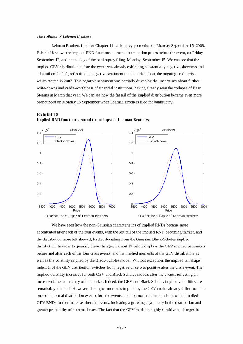
The collapse of Lehman Brothers

Lehman Brothers filed for Chapter 11 bankruptcy protection on Monday September 15, 2008.

Exhibit 18 shows the implied RND functions extracted from option prices before the event, on Friday

September 12, and on the day of the bankruptcy filing, Monday, September 15. We can see that the

implied GEV distribution before the event was already exhibiting substantially negative skewness and

a fat tail on the left, reflecting the negative sentiment in the market about the ongoing credit crisis

which started in 2007. This negative sentiment was partially driven by the uncertainty about further

write-downs and credit-worthiness of financial institutions, having already seen the collapse of Bear

Stearns in March that year. We can see how the fat tail of the implied distribution became even more

pronounced on Monday 15 September when Lehman Brothers filed for bankruptcy.

Exhibit 18 Implied RND functions around the collapse of Lehman Brothers

3500 4000 4500 5000 5500 6000 6500 70000

0.2

0.4

0.6

0.8

1

1.2

1.4x 10

-3 12-Sep-08

Price

GEV

Black-Scholes

3500 4000 4500 5000 5500 6000 6500 70000

0.2

0.4

0.6

0.8

1

1.2

1.4x 10

-3 15-Sep-08

Price

GEV

Black-Scholes

a) Before the collapse of Lehman Brothers b) After the collapse of Lehman Brothers

We have seen how the non-Gaussian characteristics of implied RNDs became more

accentuated after each of the four events, with the left tail of the implied RND becoming thicker, and

the distribution more left skewed, further deviating from the Gaussian Black-Scholes implied

distribution. In order to quantify these changes, Exhibit 19 below displays the GEV implied parameters

before and after each of the four crisis events, and the implied moments of the GEV distribution, as

well as the volatility implied by the Black-Scholes model. Without exception, the implied tail shape

index, ξ, of the GEV distribution switches from negative or zero to positive after the crisis event. The

implied volatility increases for both GEV and Black-Scholes models after the events, reflecting an

increase of the uncertainty of the market. Indeed, the GEV and Black-Scholes implied volatilities are

remarkably identical. However, the higher moments implied by the GEV model already differ from the

ones of a normal distribution even before the events, and non-normal characteristics of the implied

GEV RNDs further increase after the events, indicating a growing asymmetry in the distribution and

greater probability of extreme losses. The fact that the GEV model is highly sensitive to changes in

- 29 -

market sentiment and captures increased fear of further price falls is in line with previous studies on the

use of non-Gaussian RND analysis such as Gemmill and Saflekos [2000]. It is beyond the scope of this

article to establish whether implied GEV based RND functions can predict price falls rather than be

useful in capturing the change in market sentiment after or coincidental with the crisis event.

Exhibit 19 Summary statistics around event studies

Event Date σ ξ Implied Volatility

Implied Skewness

Implied Kurtosis

Implied Vol BS

Asian crisis 17-Oct-97 0.18 (0.003) -0.09 (0.008) 19.1% -0.60 3.47 19.8%

10-Nov-97 0.23 (0.006) +0.05 (0.024) 27.5% -1.38 6.72 26.4%

LTCM 16-Sep-98 0.31 (0.007) -0.06 (0.016) 37.6% -0.84 4.19 34.7%

16-Oct-98 0.30 (0.005) +0.03 (0.009) 39.9% -1.30 6.23 37.7%

9/11 10-Sep-01 0.22 (0.002) -0.11 (0.003) 24.3% -0.60 3.48 24.8%

12-Sep-01 0.27 (0.004) -0.05 (0.011) 28.8% -0.89 4.35 30.0%

Lehman Brothers

12-Sep-08 0.19 (0.022) +0.00 (0.054) 22.4% -0.85 4.20 22.5%

15-Sep-08 0.24 (0.013) -0.05 (0.020) 25.7% -0.99 4.75 26.8%

Notes: GEV parameters with standard errors, implied moments by the GEV based RND functions, and implied Black-Scholes volatility around crisis events.

CONCLUSIONS

We have developed a new option pricing model that is based on the GEV distribution, and

have obtained closed form solutions for the Harrison and Pliska [1981] no arbitrage equilibrium price

for the European call and put options. It was argued that the GEV density function for negative asset

returns, which in turn yielded the GEV based RND function, has great flexibility in defining the tail

shape of the latter implied by traded option price data without a priori restrictions on the class of

distributions. In particular, no a priori restriction is imposed that the GEV distribution function of

negative returns belongs to the Fréchet class with fat tails. The traded option data is used to select the

GEV RND function which displays left skewness and leptokurtosis for the underlying under the risk

neutral measure. Some recent option pricing models that aim to capture the leptokurtosis and left skew

in the RND function, in contrast, start with a specific fat tailed distribution. Other option pricing

models that attempt to overcome the drawbacks of the Black-Scholes model fail to obtain closed form

solutions or have far too many parameters.

The closed form solution for the GEV based call option pricing model has properties

analogous to the Black-Scholes price equation, especially with regard to the probability of the option of

being in or out of the money at maturity. In the GEV case, the latter is governed by the cumulative

distribution for the GEV, which is defined by the implied GEV parameters. The implications for the

probability mass in the tails of the GEV density function with switches in the tail shape parameter, ξ , is

shown to challenge the traditional understanding of tail behaviour from symmetric Gumbel class of

distributions where 99% of the rises and falls of value occur within limited volatility range and with no

skew in the probability mass. The skew in the density function in the case of positive and negative tail

- 30 -

shape values implies large one directional movements and truncated probability mass beyond a certain

value in the other direction. In other words, a simultaneous existence of infinite tails in both directions

is typically unlikely except for Gumbel class of distributions where, ofcourse, extreme moves in either

direction have non-zero but negligible probability.

From the analysis, there is a very clear indication that ξ > 0 results in a smaller probability for

a call option being in the money at maturity compared to the Black-Scholes case. In contrast, for the

put option, ξ > 0 results in a higher probability of being in the money at lower strikes when compared

to the Black-Scholes case. When applying the GEV option pricing model for the FTSE 100 index

options, it was found that the GEV based in-sample pricing biases were substantially smaller than the

ones from the Black-Scholes, for all times to maturity and at all moneyness levels. This improved

pricing accuracy was also found in out-of-sample pricing tests, when forecasting one day ahead option

prices with previous day’s parameter estimates.

We showed how the implied tail shape parameter was found to be time varying, though stable

enough to be useful in out of sample pricing. Cases of high positive ξ in the market implied density

function, associated with the GEV-Fréchet class, usually coincided with periods of market falls and

periods surrounding crisis events. For most other periods, the implied tail shape parameter indicated

Weibull or Gumbel distributions.

In the event studies surrounding particular crisis events, typically the implied tail shape

parameter ξ increases after the crisis event, which indicates that the implied GEV distributions reflect

the market sentiment of increased fear of downward moves. There is a large and growing literature on

traded option implied statistics for their capacity to incorporate market information and for forecasting

volatility and market distress (see,Giamouridis and Skiadopoulis [2010], and Poon and Granger

[2003]). Given the in sample and out of sample option pricing capabilities of the GEV model for 30

days and longer time to maturity, there is clear indication that GEV based RNDs can deliver good

results in terms of capturing market expectations of market distress beyond the 30 day horizon. These

results are in line with those in Peng, Markose and Alentorn [2010], who have found that the GEV

RND based implied volatility outperforms VIX type model free implied volatility measures for

forecasting realized volatility. However, further research is needed to establish more rigorously

whether, as noted in previous studies (Gemmill and Saflekos [2000]), the implied RND functions have

predictive power regarding downward market movements or can only reflect these moves coincidental

with the market crisis.

Future work will analyse the hedging properties of the GEV based option pricing model, and

its scope for delta hedging. Further, the option market implied tail index and the GEV based RND have

useful and interesting applications in risk management. In Markose and Alentorn [2008] the GEV

based implied RND is used to obtain the so called Extreme Economic Value at Risk (EE-VaR), in line

with the proposal to use a quantile based application of the option implied RND in Ait-Sahalia and Lo

[2000]. It has been argued that E-VaR , in contrast to historical data based VaR (sometimes called

statistical or S-VaR) is a more general risk measure since it incorporates the market’s evaluation of

risk, the demand–supply effects, and the probabilities that correspond to extreme losses (Panigirtzoglou

and Skiadopoulos [2004]). Markose and Alentorn [2008] find that the GEV RND based VaR obtained

- 31 -

from traded options can deliver better VaR performance than conventional methods. The explicit tail

shape parameter of the GEV based RND is cited as the main reason for the capacity of this new model

to flexibly and rapidly respond to extreme market movements which to date has not been adequately

dealt with by other option pricing models.

APPENDIX A Derivation of the put option price equation for ξ > 0

The derivation of the closed form solution for the put option price equation is similar to the

derivation for the call option price equation. When applying the change of variable defined in (13) to

the put option price equation, after having substituted for the price RND function g(ST) in (10), the

upper limit of integration K in the put option equation becomes H as defined in (16), while the lower

limit of integration in the put option equation becomes ( ) σµξ /11 −+=h . Using these new limits of

integration we have:

( ) ( ) ( ) ( )

+−−−−= ∫∫−− −−−−−−− H

h

yt

H

h

ytTrt dyeySKdyeyy

SeP

ξξ ξξ

ξσµ

ξσ

ξ/1/1 /11/110)( 1

1

+−−−−= 210 1

1 ψξσµψ

ξσ

ξ tSKS

(A-1)

Evaluating the first integral in (A-1) yields:

( ) ( ) ( )[ ] ( ) ( )( )ξξξξξξψ ξ /1/1/1/1/11

1

−−−− −−−−−− −=== ∫hHH

hyH

h

y eeedyey (A-2)

To solve the second integral in (A.1), consider the change of variable ξ/1−= yt , and ξ−= ty

dttdy ξξ −−−= 1 , which yields:

( ) dtetdtettdtetH

h

tH

h

tH

h

t

∫∫∫−

−

−

−

−

−

−−−−−−−−− −=−==ξ

ξ

ξ

ξ

ξ

ξ

ξξξξ ξξψ/

/

/

/

/

/

1)1(12 (A-3)

We can solve this integral directly by using the definition of the generalized Gamma function:

∫−−=Γ=Γ−Γ 1

0

11010 ),,(),(),(

z

z

ta dtetzzazaza (A-4)

and we obtain the following result:

( ) ( )ξξξξ ξξψ /1/1/1/12 ,,1exp −−−− −Γ−=−= ∫ Hhdyyy

H

h (A-5)

Combining results for 1ψ and 2ψ and rearranging, we obtain a closed form solution for the put option

equation:

( ) ( )( ) ( )

−Γ−−+−−−= −−−−−−−− −−−− ξξξξσξσµ

ξξξξ /1/1)( ,,11)(/1/1/1/1

HheeSeeKeKP hHt

HhtTrt

(A-6)

- 32 -

APPENDIX B Derivation of the call option price equation for ξ = 0

The derivation of the closed form solution of the call option price when ξ = 0 follows a similar

procedure to the one when ξ ≠ 0. By assuming that negative returns are distributed following the

standardised GEV distribution when ξ = 0 given in (3.b), and applying the formula in (9) we obtain the

RND function of the underlying price g(ST) in terms of the standardized GEV density function given in

equation (3.b) as follows:

( ) ( )

−−−

−−=σ

µσ

µσ

TT

tT

LL

SSg expexpexp

1)( (B-1)

Substituting g(ST) in (B.1) into the call price equation in (4), we have:

( ) ( ) ( ) ( )∫

∞−−

−−−

−−−=K T

TT

tT

tTrt dS

LL

SKSeKC

σµ

σµ

σexpexpexp

1)( (B-2)

Consider the change of variable:

( )

+−=−−= µ

σσµ

11

t

TT

S

SLy (B-3)

Under this change of variable, the underlying price ST and dST can be written in terms of y as follows:

( )ySS tT σµ +−= 1 and dySdS tT σ= (B-4)

Also, the density function in (B-1) for the underlying price at maturity in terms of y becomes:

))exp(exp(1

)( yyS

ygt

−=σ

(B-5)

Note now that under the change of variable the lower limit of integration for the call option equation in

(B.2) becomes:

+−= µ

σ1

1

tS

KH (B-6)

while the upper limit of integration in (B-2) remains infinity. Substituting for ST and dST as defined in

(B-4) into (B-2), using the new limits of integration, and rearranging we have:

- 33 -

( )( )

( )( )( )( ) 21

)(

1

))exp(exp(1)exp(exp(

))exp(exp(1

ψµψσ

µσ

σµ

KSS

dyyyKSdyyyyS

dyyyKySeC

tt

HtHt

H ttTr

t

−−+=

−−−+−=

−−+−=

∫∫

∫∞∞

∞−

(B-7)

The integral 1ψ in (B-7) above can be evaluated in terms of the incomplete gamma function, by

applying the change of variable t = exp(y) and integrating by parts, yielding the following solution:

[ ]

))exp(,0())exp(exp(

))exp(,0())exp(exp())exp(exp(1

HH

yydyyyy HH

Γ+−=

Γ−−−=−= ∞∞

∫ψ (B-8)

The solution of integral 2ψ in (B-7) is:

( )[ ] ))exp(exp()exp(exp)exp(exp(2 Hydyyy HH−=−−=−= ∞∞

∫ψ (B-9)

Combining results for 1ψ and 2ψ and rearranging, we obtain a closed form for the GEV call option

price:

( )( )[ ]HH eHet

tTrt eKeeSeKC −−−− −Γ++−= ),0(1)( )( σσµ (B-10)

Following a similar procedure, the closed form solution of the GEV model for the put option price

when ξ = 0 is found to be:

( ) ( ) ( )( )[ ]),,0(1)( )( Hheet

eetTrt eeeeSeeKeKP

HhHh

Γ+−+−−−= −−−−−− σσµ (B-11)

APPENDIX C Simplification for deep in the money options

The GEV option pricing equation in (22) can be simplified for the special case when the call

option is deep in the money, i.e St >> K . In that case, the terms involving H can be simplified, and as

1/1

→−− ξHe , it implies that 0/1 →− ξH . Substituting these approximations into the call option

equation in (22) and rearranging, the call option price becomes a linear function of K:

( )( )

−

−Γ−+−= −− KSeKC ttTr

t ξξσµ 111)( )( (C-1)

The mean of the standardized GEV negative returns, LT, distribution is given by (see Dowd, 2002, p.273):

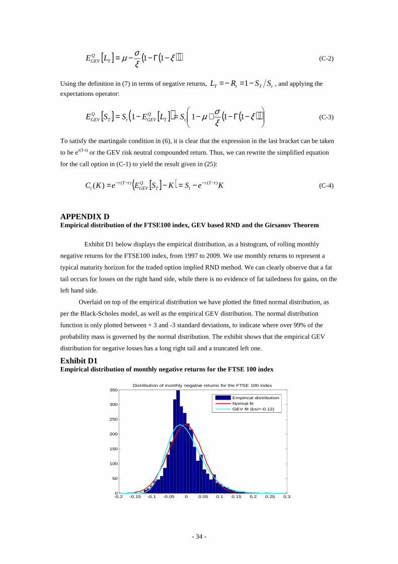
- 34 -

[ ] ( )( )ξξσµ −Γ−−= 11T

QGEV LE (C-2)

Using the definition in (7) in terms of negative returns, tTtT SSRL −=−= 1 , and applying the

expectations operator:

[ ] [ ]( ) ( )( )

−Γ−+−=−= ξξσµ 1111 tT

QGEVtT

QGEV SLESSE (C-3)

To satisfy the martingale condition in (6), it is clear that the expression in the last bracket can be taken

to be er(T-t) or the GEV risk neutral compounded return. Thus, we can rewrite the simplified equation

for the call option in (C-1) to yield the result given in (25):

[ ]( ) KeSKSEeKC tTrtT

QGEV

tTrt

)()()( −−−− −=−= (C-4)

APPENDIX D Empirical distribution of the FTSE100 index, GEV based RND and the Girsanov Theorem

Exhibit D1 below displays the empirical distribution, as a histogram, of rolling monthly

negative returns for the FTSE100 index, from 1997 to 2009. We use monthly returns to represent a

typical maturity horizon for the traded option implied RND method. We can clearly observe that a fat

tail occurs for losses on the right hand side, while there is no evidence of fat tailedness for gains, on the

left hand side.

Overlaid on top of the empirical distribution we have plotted the fitted normal distribution, as

per the Black-Scholes model, as well as the empirical GEV distribution. The normal distribution

function is only plotted between + 3 and -3 standard deviations, to indicate where over 99% of the

probability mass is governed by the normal distribution. The exhibit shows that the empirical GEV

distribution for negative losses has a long right tail and a truncated left one.

Exhibit D1 Empirical distribution of monthly negative returns for the FTSE 100 index

-0.2 -0.15 -0.1 -0.05 0 0.05 0.1 0.15 0.2 0.25 0.30

50

100

150

200

250

300

350Distribution of monthly negative returns for the FTSE 100 index

Empirical distribution

Normal fitGEV fit (ksi=-0.12)

- 35 -

We need to verify that the Q-impossible events implied by the conditions for the GEV RND

function in equation (11) are not P-possible.

Exhibit D2 Time series of truncation points, and realised rolling monthly FTSE 100 returns

-100%

-80%

-60%

-40%

-20%

0%

20%

40%

60%

80%

100%

Jan1

997

Jan1

998

Jan1

999

Jan2

000

Jan2

001

Jan2

002

Jan2

003

Jan2

004

Jan2

005

Jan2

006

Jan2

007

Jan2

008

Jan2

009

Loss

es

Right tail truncation Left tail truncation Monthly rolling FTSE100 returns

We obtain the daily implied tail shape parameters, ξ, and the precise truncation values that are

obtained in terms of the upper bound (maximum gain, left tail or gains) and lower bound (maximum

loss, right tail for losses). This has been plotted in Exhibit D2 along with the realized negative returns

which is centred on zero percentage returns. Note that less stringent truncation values for returns in

excess of +/- 100% are not shown in the plot. The data for the upper and lower truncations values

visible in the plot constitute only 45% of all possible days and on a large proportion of other days the

Q-possible range of percentage gains and losses were well beyond even the +/- 100% band. As can be

seen at no time does the realized returns violate the truncation points given by the implied tail shape

parameter, ξ, for the GEV based RND.

ENDNOTES This article has benefited greatly from detailed inputs from Stephen Figlewski and an anonymous

referee. We are grateful for comments from Radu Tunaru, George Skidiapoulos, Christoph Schleicher,

Thomas Lux, Peter Winker and Chris Schwab. Discussions with participants have been useful at

conferences at MAF 2010 in Ravello, FMA 2005 in Siena, CEF 2005 in Washington and

Computational Finance workshop at the CAU University of Kiel.

- 36 -

REFERENCES Abadir, K., and M. Rockinger. “Density-Embedding Functions.” Working paper, HEC, 1997. Ait-Sahalia,Y. and A.W. Lo. “Nonparametric Estimation of State-Price Densities Implicit in Financial Asset Prices.” Journal of Finance, 53 (1998), pp. 499-547. _______________________. “Nonparametric Risk Management and Implied Risk Aversion.” Journal of Econometrics, 94 (2000), pp. 9-51. Aparicio, S. D., and S.D. Hodges. “Implied Risk-Neutral Distribution: A Comparison of Estimation Methods.” FORC Preprint, University of Warwick, 1998. Black, F. and M. Scholes. “The Pricing of Options and Corporate Liabilities.” Journal of PoliticalEconomy, 81 (1973), pp. 637-659. Bliss, R. and N. Panigirtzoglou. “Testing the Stability of Implied Probability Density Functions.” Journal of Banking and Finance, 26 (2002), pp. 381-422. Bliss, R., and N. Panigirtzoglou. “Option-Implied Risk Aversion Estimates.” Journal of Finance, 59 (2004), pp. 407–446. Breeden, D. and R. Litzenberger. “Prices of State-Contingent Claims Implicit in Option Prices.” Journal of Business, 51 (1978), pp. 621-651. Buchen, P. W. and M. Kelly. “The maximum entropy distribution of an asset inferred from option prices.” Journal of Financial and Quantitative Analysis, 31 (1996), pp. 143-159. Corrado, C.J. “Option pricing based on the Generalized Lambda Distribution.” Journal of Futures Markets, 21 (2001), pp. 213–236. Corrado, C.J. and T. Su. “Skewness and Kurtosis in S&P 500 Index Returns Implied by Option Prices.” The Journal of Financial Research, 19 (1996), pp. 175-192. Corrado, C.J. and T. Su. “Implied Volatility Skews and Stock Index Skewness and Kurtosis Implied by S&P500 Index Option Prices.” Journal of Derivatives, 4 (1997), pp. 8-19. de Jong, C. and R. Huisman. “From Skews to a Skewed-t.” ERIM Report Series Reference No. ERS-2000-12-F&A, 2000. Dowd, K. Measuring Market Risk. New York: John Wiley and Sons, 2002. Embrechts, P., C. Klüppelberg and T. Mikosch. Modelling Extremal Events for Insurance and Finance. Berlin: Springer, 1997. Embrechts P., S. Resnick and G. Samorodnitsky. “Extreme value theory as a risk management tool.” North American Actuarial Journal, 3 (1999), pp. 30-41. Embrechts, P. “Extreme Value Theory: Potential and Limitations as an Integrated Risk Management Tool.” Derivatives Use, Trading & Regulation, 6 (2000), pp. 449-456. Figlewski, S. “Assessing the Incremental Value of Option Pricing Theory Relative to an Informationally Passive Benchmark.” Journal of Derivatives Vol. 10, No. 3 (Fall 2002), pp. 80-96. Figlewski, S. “Estimating the Implied Risk Neutral Density for the U.S. Market Portfolio”, 2010. In T. Bollerslev, J. R. Russell and M. Watson, eds: Volatility and Time Series Econometrics: Essays in Honor of Robert F. Engle, Oxford, UK: Oxford University Press.

- 37 -

Fisher, R.A. and L.H.C. Tippett. “Limiting forms of the frequency distributions of the largest or smallest member of a sample.” Proceedings of the Cambridge Philosophical Society, 24 (1928), pp. 180-190. Gemmill G, and A. Saflekos. “How Useful are Implied Distributions? Evidence from Stock-Index Options.” Journal of Derivatives, 7 (2000), pp. 83-98. Giamouridis, D., and G. Skiadopoulos. “The Informational Content of Financial Options for Quantitative Asset Management: A review”, 2010. In B. Scherer and K. Winston, eds: Handbook of Quantitative Asset Management, (Oxford University Press), forthcoming. Harrison, J. M. and S. R. Pliska. “Martingales and stochastic integrals in the theory of continuous trading.” Stochastic Processes Applications, 11 (1981), pp. 215-260. Jackwerth, J. C. and M. Rubinstein. “Recovering Probability Distributions from Options Prices.” Journal of Finance, 51 (1996), pp. 1611-1631. Jackwerth, J. C. “Option-Implied Risk-Neutral Distributions and Implied Binomial Trees: A Literature Review”. Journal of Derivatives, 7 (1999), pp. 66-82. Jenkinson, A. F. “The frequency distribution of the annual maximum (or minimum) values of meteorological elements.” Quarterly Journal of the Royal Meteorological Society, 87 (1955), pp. 158-171. Lux, T. and D. Sornette. “On Rational Bubbles and Fat Tails.” Journal of Money, Credit and Banking, 34 (2002), pp. 589-610. Madan, D., P. Carr and E. Chang. “The variance gamma process and option pricing.” European Finance Review, 2 (1998), pp. 79-105. Mandelbrot B. “The Variation of Certain Speculative Prices.” Journal of Business, 36 (1963), pp. 394-419. Markose, S.M., and A. Alentorn. “Generalized Extreme Value Distribution and Extreme Economic Value at Risk (E-EVaR).” In Computational Methods in Financial Engineering edited by EJ Kontoghiorghes, B. Rustem and P. Winker in honour of Manfred Gilli, Springer Verlag, 2008. Matache, A.M., P.A. Nitsche and C. Schwab. “Wavelet Galerkin Pricing of American Options on Levy Driven Assets.” Working paper, ETH Zürich, 2004. Mc Neil , A.J. “Extreme Value Theory for Risk Managers.” Internal Modelling and CAD II, published by RISK Books, pp. 93-113, 1999. Melick, W. R. and C. P. Thomas. “Recovering an Asset’s Implied PDF from Option Prices: An application to Crude Oil during the Gulf Crisis.” Journal of Financial and Quantitative Analysis, 32 (1997), pp. 91-115. Neftci, S. An Introduction to the Mathematics of Financial Derivatives. San Diego: Academic Press Advanced Finance, 2000. Panigirtzoglou, N. and G. Skiadopoulos. “A New Approach to Modelling the Dynamics of Implied Distributions: Theory and Evidence from the S&P 500 Options.” Journal of Banking and Finance, 28 (2004), pp. 1499-1520. Peng, Y., S. Markose and A. Alentorn. “Volatility Forecasting with V-FTSE. Model Free and GEV Implied Volatility Indices.” Economics Dept. University of Essex, Mimeo, 2010. Poon, S.-H., and C. W.J., Granger. “Forecasting volatility in financial markets: A review.” Journal of Economic Literature, 26 (2003), pp. 478-539.

- 38 -

Quintos, C., Z. Fan, and P. C. B. Phillips. “Structural Change Tests in Tail Behavior and the Asian Crisis.” Review of Economic Studies, 68 (2001), pp. 633–663. Reiss, R. D. and M. Thomas. Statistical Analysis of Extreme Values, 2nd ed. Basel: Birkhäuser, 2001. Ritchey, R. J. “Call Option Valuation for Discrete Normal Mixtures.” Journal of Financial Research, 13 (1990), pp. 285-296. Rocco, M. “Extreme Value Theory for Finance: A Survey.” University of Bergamo, Department of Mathematics, Statistics and Informatics Working Paper N. 3, 2010. Rubinstein, M. “Nonparametric Tests of Alternative Option Pricing Models Using All Reported Trades and Quotes on the 30 Most Active CBOE Option Classes from August 23, 1976 through August 31, 1978.” Journal of Finance, 40 (1985), pp. 455-480. Savickas, R. “A simple option-pricing formula”. The Financial Review, 37 (2002), 207-226. Shimko, D. “Bounds of Probability.” Risk, 6 (1993), pp. 33-37. von Mises, R. “La Distribution de la Plus Grande de n Valeurs.” 1936. In Selected Papers of Richard von Mises, 2, pp. 271-294. Providence, RI: American Mathematical Society.