Journal of Modern Applied StatisticalMethods

Volume 8 | Issue 1 Article 22

5-1-2009

A New Approximate Bayesian Approach forDecision Making About the Variance of a GaussianDistribution Versus the Classical ApproachVincent A. R. CamaraUniversity of South Florida, gvcamara@ij.net

Follow this and additional works at: http://digitalcommons.wayne.edu/jmasm

Part of the Applied Statistics Commons, Social and Behavioral Sciences Commons, and theStatistical Theory Commons

This Regular Article is brought to you for free and open access by the Open Access Journals at DigitalCommons@WayneState. It has been accepted forinclusion in Journal of Modern Applied Statistical Methods by an authorized editor of DigitalCommons@WayneState.

Recommended CitationCamara, Vincent A. R. (2009) "A New Approximate Bayesian Approach for Decision Making About the Variance of a GaussianDistribution Versus the Classical Approach," Journal of Modern Applied Statistical Methods: Vol. 8 : Iss. 1 , Article 22.DOI: 10.22237/jmasm/1241137260Available at: http://digitalcommons.wayne.edu/jmasm/vol8/iss1/22

Journal of Modern Applied Statistical Methods Copyright © 2009 JMASM, Inc. May 2009, Vol. 8, No. 1, 237-247 1538 – 9472/09/$95.00

237

A New Approximate Bayesian Approach for Decision Making About the Variance of a Gaussian Distribution Versus the Classical Approach

Vincent A. R. Camara

University of South Florida

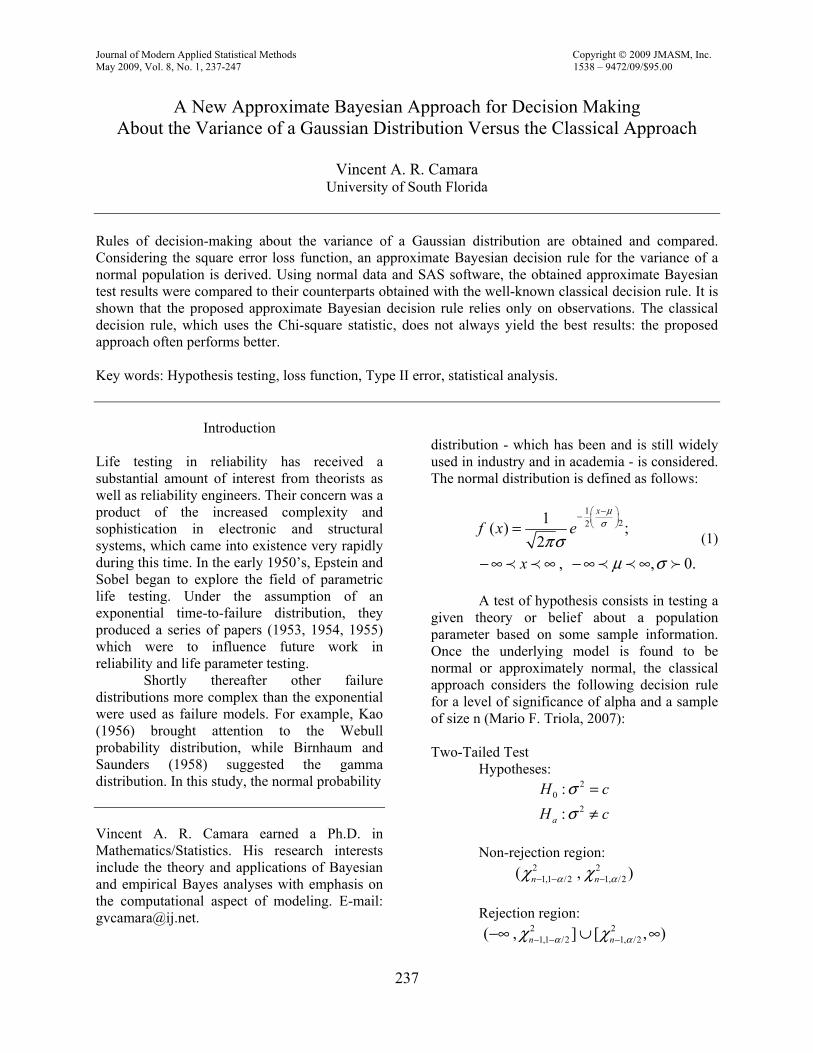
Rules of decision-making about the variance of a Gaussian distribution are obtained and compared. Considering the square error loss function, an approximate Bayesian decision rule for the variance of a normal population is derived. Using normal data and SAS software, the obtained approximate Bayesian test results were compared to their counterparts obtained with the well-known classical decision rule. It is shown that the proposed approximate Bayesian decision rule relies only on observations. The classical decision rule, which uses the Chi-square statistic, does not always yield the best results: the proposed approach often performs better. Key words: Hypothesis testing, loss function, Type II error, statistical analysis.

Introduction Life testing in reliability has received a substantial amount of interest from theorists as well as reliability engineers. Their concern was a product of the increased complexity and sophistication in electronic and structural systems, which came into existence very rapidly during this time. In the early 1950’s, Epstein and Sobel began to explore the field of parametric life testing. Under the assumption of an exponential time-to-failure distribution, they produced a series of papers (1953, 1954, 1955) which were to influence future work in reliability and life parameter testing.

Shortly thereafter other failure distributions more complex than the exponential were used as failure models. For example, Kao (1956) brought attention to the Webull probability distribution, while Birnhaum and Saunders (1958) suggested the gamma distribution. In this study, the normal probability Vincent A. R. Camara earned a Ph.D. in Mathematics/Statistics. His research interests include the theory and applications of Bayesian and empirical Bayes analyses with emphasis on the computational aspect of modeling. E-mail: gvcamara@ij.net.

distribution - which has been and is still widely used in industry and in academia - is considered. The normal distribution is defined as follows:

1221

( ) ;2

, , 0.

x

f x e

x

μσ

πσμ σ

− − =

− ∞ ∞ − ∞ ∞ (1)

A test of hypothesis consists in testing a

given theory or belief about a population parameter based on some sample information. Once the underlying model is found to be normal or approximately normal, the classical approach considers the following decision rule for a level of significance of alpha and a sample of size n (Mario F. Triola, 2007): Two-Tailed Test

Hypotheses: 2

0 :H cσ = 2:aH cσ ≠

Non-rejection region:

2 21,1 /2 1, /2( , )n nα αχ χ− − −

Rejection region:

2 21,1 /2 1, /2( , ] [ , )n nα αχ χ− − −−∞ ∪ ∞

BAYESIAN APPROXIMATION FOR THE VARIANCE OF A GAUSSIAN DISTRIBUTION

238

Right Tailed Test Hypotheses:

20 :H cσ =

2:aH cσ

Non-rejection region:

21,( , )n αχ −−∞

Rejection region:

21,[ , )n αχ − ∞

Left Tailed Test

Hypotheses: 2

0 :H cσ = 2:aH cσ

Non-rejection region:

21,( , )n αχ − ∞

Rejection region:

21,( , ]n αχ −−∞

The Chi-square test statistic that is used to conduct the above tests will be denoted by Chi, with:

2

2

( 1)n sChiσ−= .

Methodology

Although no specific analytical procedure exists that allows identification of the appropriate loss function to be used in Bayesian analysis, the most commonly used is the square error loss function. One of the reasons for selecting this loss function is due to its analytical tractability in Bayesian analysis. The square error loss function places a small weight on estimates near the true value and proportionately more weight on extreme deviation from the true value of the parameter. The square error loss is defined

(2)

The use of the square error loss function along with a suitable approximation of the Pareto prior leads to the following approximate Bayesian confidence bounds for the normal population variance (Camara, 2003):

2

2

1( )

( )

2 2ln( / 2)

n

ii

SE

xL

nο

μ

α=

−=

− −

2

2

1( )

( )

2 2ln(1 / 2)

n

ii

SE

xU

nσ

μ

α=

−=

− − −

or

2

_2

1( )

( )

2 2ln( / 2)

n

ii

SE

x xL

nο α=

−=

− −

2

_2

1( )

( )

2 2ln(1 / 2)

n

ii

SE

x xU

nσ α=

−=

− − −

(3)

To obtain the approximate Bayesian

decision rule for the variance of a normal population, the close relationship that exists between confidence intervals and hypothesis testing is used. Considering the above mentioned approximate Bayesian confidence intervals along with the test statistic Chi, the following approximate Bayesian decision rule is derived: Two-Tailed Test

Hypotheses: 2

0 :H cσ = 2:aH cσ ≠

Non-rejection region:

2 2 ln(1 / 2) , 2 2ln( / 2)( )n nα α− − − − −

Rejection region:

( , 2 2 ln(1 / 2)] [ 2 2 ln( / 2), )n nα α−∞ − − − ∪ − − ∞

2

),(

−= θθθθ

ΛΛ

SEL

CAMARA

239

Right Tailed Test Hypotheses:

20 :H cσ =

2:aH cσ

Non-rejection region:

( , 2 2 ln( ))n α−∞ − −

Rejection region: [ 2 2 ln( ), )n α− − ∞

Left Tailed Test

Hypotheses: 2

0 :H cσ = 2:aH cσ

Non-rejection region:

( 2 2 ln( ), )n α− − ∞

Rejection region: ( , 2 2 ln( )]n α−∞ − −

To compare the classical and

approximate Bayesian decision rules and evaluate their performances, the absolute difference, AD, between the parameter and the claim is used and is defined by:

AD Parameter Claim= −

From the calculated results of the absolute difference between the parameter and the claim, the following are able to be concluded:

• For a reasonably large value of AD, the test that will perform better than its counterpart will be the one that will reject the null hypothesis.

• For a reasonably small value of AD, the test that will perform better than its counterpart will be the one that will fail to reject the null hypothesis.

• A test and its counterpart will perform equally well, if both reject the null hypothesis for a reasonably large value of AD or both fail to reject the null

hypothesis for a reasonably small value of AD.

• A test and its counterpart will perform poorly if, for a reasonably large value of AD, both fail to reject the null hypothesis, or both reject the null hypothesis for a reasonably small value of AD.

Results

In order to compare the proposed approximate Bayesian decision rule with the classical approach, samples obtained from normally distributed populations (e.g., 1, 2, 3, .4, 7) as well as approximately normal populations (e.g., 5, 6) are considered. SAS software was used to obtain the normal population parameters corresponding to each sample data set.

The observed value, which is the value of the test statistic Chi under the assumption that the null hypothesis is true, will be denoted by Chio. If this observed value, Chio, falls into the rejection region, the null hypothesis will be rejected at a level of significance selected beforehand. If the observed value falls into the non-rejection region, the null hypothesis will not be rejected at the selected level of significance Data Set #1: 24, 28, 22, 25, 24, 22, 29, 26, 25, 28, 19, 29 (Mann, 1998, p. 504). Normal population distribution obtained with SAS:

( 25.083, 3.1176)N μ σ= = . The population and sample variances are:

2 9.71943σ = , and 2 9.719696s = . For the following test of hypothesis,

20 :H cσ = ,

2:aH cσ ≠ ,

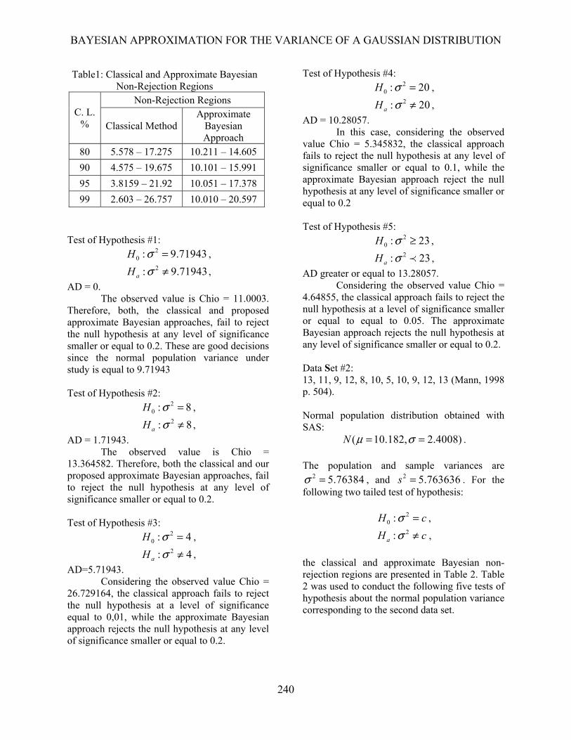
the classical and approximate Bayesian non-rejection regions are presented in Table 1. Table 1 was used to conduct the following five tests of hypothesis about the normal population variance corresponding to the first data set.

BAYESIAN APPROXIMATION FOR THE VARIANCE OF A GAUSSIAN DISTRIBUTION

240

Test of Hypothesis #1:

20 : 9.71943H σ = ,

2: 9.71943aH σ ≠ ,

AD = 0. The observed value is Chio = 11.0003.

Therefore, both, the classical and proposed approximate Bayesian approaches, fail to reject the null hypothesis at any level of significance smaller or equal to 0.2. These are good decisions since the normal population variance under study is equal to 9.71943 Test of Hypothesis #2:

20 : 8H σ = ,

2: 8aH σ ≠ ,

AD = 1.71943. The observed value is Chio =

13.364582. Therefore, both the classical and our proposed approximate Bayesian approaches, fail to reject the null hypothesis at any level of significance smaller or equal to 0.2. Test of Hypothesis #3:

20 : 4H σ = ,

2: 4aH σ ≠ ,

AD=5.71943. Considering the observed value Chio =

26.729164, the classical approach fails to reject the null hypothesis at a level of significance equal to 0,01, while the approximate Bayesian approach rejects the null hypothesis at any level of significance smaller or equal to 0.2.

Test of Hypothesis #4: 2

0 : 20H σ = , 2: 20aH σ ≠ ,

AD = 10.28057. In this case, considering the observed

value Chio = 5.345832, the classical approach fails to reject the null hypothesis at any level of significance smaller or equal to 0.1, while the approximate Bayesian approach reject the null hypothesis at any level of significance smaller or equal to 0.2 Test of Hypothesis #5:

20 : 23H σ ≥ ,

2: 23aH σ ,

AD greater or equal to 13.28057. Considering the observed value Chio =

4.64855, the classical approach fails to reject the null hypothesis at a level of significance smaller or equal to equal to 0.05. The approximate Bayesian approach rejects the null hypothesis at any level of significance smaller or equal to 0.2. Data Set #2: 13, 11, 9, 12, 8, 10, 5, 10, 9, 12, 13 (Mann, 1998 p. 504). Normal population distribution obtained with SAS:

( 10.182, 2.4008)N μ σ= = . The population and sample variances are

2 5.76384σ = , and 2 5.763636s = . For the following two tailed test of hypothesis:

20 :H cσ = ,

2:aH cσ ≠ ,

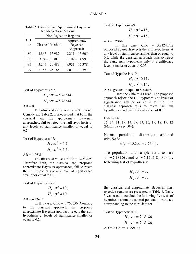
the classical and approximate Bayesian non-rejection regions are presented in Table 2. Table 2 was used to conduct the following five tests of hypothesis about the normal population variance corresponding to the second data set.

Table1: Classical and Approximate Bayesian Non-Rejection Regions

C. L. %

Non-Rejection Regions

Classical Method Approximate

Bayesian Approach

80 5.578 – 17.275 10.211 – 14.605

90 4.575 – 19.675 10.101 – 15.991

95 3.8159 – 21.92 10.051 – 17.378

99 2.603 – 26.757 10.010 – 20.597

CAMARA

241

Test of Hypothesis #6:

20 : 5.76384H σ = ,

2: 5.76384aH σ ≠ ,

AD = 0. The observed value is Chio = 9.999645.

Considering Table 2, it is observed that both, the classical and the approximate Bayesian approaches, fail to reject the null hypothesis at any levels of significance smaller of equal to 0.2. Test of Hypothesis #7:

20 : 4.5H σ = ,

2: 4.5aH σ ≠ ,

AD = 1.26384. The observed value is Chio = 12.80808.

Therefore both, the classical and proposed approximate Bayesian approaches, fail to reject the null hypothesis at any level of significance smaller or equal to 0.2. Test of Hypothesis #8:

20 : 10H σ = ,

2: 10aH σ ≠ ,

AD = 4.23616. In this case, Chio = 5.763636. Contrary

to the classical approach, the proposed approximate Bayesian approach rejects the null hypothesis at levels of significance smaller or equal to 0.2.

Test of Hypothesis #9: 2

0 : 15H σ = , 2: 15aH σ ≠ ,

AD = 9.23616. In this case, Chio = 3.8424.The

proposed approach rejects the null hypothesis at any level of significance smaller than or equal to 0.2, while the classical approach fails to reject the same null hypothesis only at significance levels smaller or equal to 0.05. Test of Hypothesis #10:

20 : 14H σ ≥ ,

2: 14aH σ ,

AD is greater or equal to 8.23616. Here the Chio = 4.11688. The proposed

approach rejects the null hypothesis at levels of significance smaller or equal to 0.2. The classical approach fails to reject the null hypothesis at a level of significance of 0.05. Data Set #3: 16, 14, 11, 19, 14, 17, 13, 16, 17, 18, 19, 12 (Mann, 1998 p. 504). Normal population distribution obtained with SAS:

( 15.5, 2.6799)N μ σ= = . The population and sample variances are

2 7.18186σ = , and 2 7.181818s = . For the following test of hypothesis:

20 :H cσ = ,

2:aH cσ ≠ ,

the classical and approximate Bayesian non-rejection regions are presented in Table 3. Table 3 was used to conduct the following five tests of hypothesis about the normal population variance corresponding to the third data set. Test of Hypothesis #11:

20 : 7.18186H σ = ,

2: 7.18186aH σ ≠ ,

AD = 0, Chio=10.999935.

Table 2: Classical and Approximate Bayesian Non-Rejection Regions

C. L. %

Non-Rejection Regions

Classical Method Approximate

Bayesian Approach

80 4.865 – 15.987 9.211 – 13.605

90 3.94 – 18.307 9.102 – 14.991

95 3.247 – 20.483 9.051 – 16.378

99 2.156 – 25.188 9.010 – 19.597

BAYESIAN APPROXIMATION FOR THE VARIANCE OF A GAUSSIAN DISTRIBUTION

242

Both, the classical and proposed approximate Bayesian approaches, fail to reject the null hypothesis at any level of significance smaller or equal to 0.2. Test of Hypothesis #12:

20 : 6H σ = ,

2: 6aH σ ≠ ,

AD = 1.18186. The observed value is Chio =

13.166666. Therefore both, the classical and proposed approximate Bayesian approaches, fail to reject the null hypothesis at any level of significance smaller or equal to 0.2 Test of Hypothesis #13:

20 : 14H σ = ,

2: 14aH σ ≠ ,

AD = 6.81814, Chio = 5.64285. Contrary the classical approach, the

proposed approximate Bayesian approach rejects the null hypothesis at levels of significance respectively small or equal to 0.2. Test of Hypothesis #14:

20 : 18H σ = ,

2: 18aH σ ≠ ,

AD=10.81814, Chio=4.388888. The proposed approximate Bayesian

approach rejects the null hypothesis at any significance level smaller or equal to 0.2. The classical approach fails to reject the null hypothesis at levels of significance respectively smaller or equal to 0.05.

Test of Hypothesis #15: 2

0 : 17H σ ≥ , 2: 17aH σ ,

AD is greater or equal to 9.81814. The observed value Chio = 4.647058.

Based on Table 3, the proposed decision rule rejects the null hypothesis at any level of significance smaller or equal to 0.1. The classical approach fails to reject the null hypothesis at levels of significance smaller or equal 0.05. Data Set #4: 27, 31, 25, 33, 21, 35, 30, 26, 25, 31, 33, 30, 28 (Mann, 1998 p. 504). Normal population distribution obtained with SAS:

( 28.846, 3.9549)N μ σ= = The population and sample variances are

2 15.64123σ = , and 2 15.641025s = . For the following test of hypothesis:

20 :H cσ = ,

2:aH cσ ≠ ,

the classical and approximate Bayesian non-rejection regions are presented in Table 4. Table 4 was used to conduct the following five tests of hypothesis about the normal population variance corresponding to the fourth data set.

Table 3: Classical and Approximate Bayesian Non-Rejection Regions

C. L. %

Non-Rejection Regions

Classical Method Approximate

Bayesian Approach

80 5.578 – 17.275 10.211 – 14.605

90 4.575 – 19.675 10.103 – 15.991

95 3.8159 – 21.92 10.051 – 17.378

99 2.603 – 26.757 10.010 – 20.597

Table 4: Classical and Approximate Bayesian Non-Rejection Regions

C. L. %

Non-Rejection Regions

Classical Method Approximate

Bayesian Approach

80 6.304 – 18.549 11.211 – 15.605

90 5.226 – 21.026 11.103 – 16.991

95 4.404 - 23.337 11.051 – 18.378

99 3.074 – 28.300 11.010 – 21.597

CAMARA

243

Test of Hypothesis #16: 2

0 : 15.64123H σ = , 2: 15.64123aH σ ≠ ,

AD = 0, Chio=11.999842. Both, the classical and proposed

approximate Bayesian approaches, fail to reject the null hypothesis at any level of significance smaller or equal to 0.2. Test of Hypothesis #17:

20 : 16.5H σ = ,

2: 16.5aH σ ≠ ,

AD = 0.85877. The observed value is Chio =

11.3752909. Therefore both, the classical and proposed approximate Bayesian approaches, fail to reject the null hypothesis at any level of significance smaller or equal to 0.2. Test of Hypothesis #18:

20 : 30H σ = ,

2: 30aH σ ≠ ,

AD = 14.35877, Chio = 6.2564 The classical approach fails to rejects

the null hypothesis at a level of significance smaller or equal to 0.1. The proposed decision rule rejects the null hypothesis for any level of significance smaller or equal to 0.2. Test of Hypothesis #19:

20 : 8H σ = ,

2: 8aH σ ≠ ,

AD = 7.64123, Chio = 23.461536. The proposed approximate Bayesian

approach rejects the null hypothesis at levels of significance smaller or equal to 0.2. The classical approach fails to reject the null hypothesis at a level of significance of 0.01. Test of Hypothesis #20:

20 : 25H σ ≥ ,

2: 25aH σ ,

AD=9.35877, Chio=7.50779. Based on Table 4, the classical approach

fails to reject the null hypothesis at any significance level smaller or equal to 0.1. The

proposed approximate Bayesian decision rule rejects the null hypothesis for any level of significance smaller or equal to 0.1. Data Set #5: 52, 33, 42, 44, 41, 50, 44, 51, 45, 38, 37, 40, 44, 50, 43 (McClave & Sincich, 1997 p. 301). Normal population distribution obtained with SAS:

( 43.6, 5.4746)N μ σ= = The population and sample variances are

2 29.97124σ = , and 2 29.971428s = . For the following test of hypothesis:

2:aH cσ ≠ , 2

0 :H cσ = , the classical and approximate Bayesian non-rejection regions are presented in Table 5. Table 5 was used to conduct the following five tests of hypothesis about the normal population variance corresponding to the fifth data set. Test of Hypothesis #21:

20 : 29.97124H σ = ,

2: 29.97124aH σ ≠ ,

AD = 0, Chio = 14.000882. Both, the classical and the proposed

approximate Bayesian approaches, fail to reject the null hypothesis at any level of significance smaller or equal to 0.2.

Table 5: Classical and Approximate Bayesian Non-Rejection Regions

C. L. %

Non-Rejection Regions

Classical Method Approximate

Bayesian Approach

80 7.790–21.064 13.211–17.605

90 6.571–23.685 13.103–18.991

95 5.629–26.119 13.051–20.378

99 4.075–31.319 13.010–23.597

BAYESIAN APPROXIMATION FOR THE VARIANCE OF A GAUSSIAN DISTRIBUTION

244

Test of Hypothesis #22: 2

0 : 31.5H σ = , 2: 31.5aH σ ≠ ,

AD = 1.52876. The observed value is Chio =

13.32063467. Therefore both, the classical and proposed approximate Bayesian approaches, fail to reject the null hypothesis at any level of significance smaller or equal to 0.2 Test of Hypothesis #23:

20 : 60H σ = ,

2: 60aH σ ≠ ,

AD = 30.02876, Chio = 6.99333. The proposed approximate Bayesian

approach rejects the null hypothesis at levels of significance smaller or equal to 0.2. The classical approach fails to reject the null hypothesis at any level of significance smaller or equal to 0.1. Test of Hypothesis #24:

20 : 17H σ = ,

2: 17aH σ ≠ ,

AD = 12.97124, Chio = 24.682352. The classical approach fails to reject the

null hypothesis at any level of significance smaller or equal to 0.05, while the proposed approximate Bayesian approach rejects the null hypothesis at levels of significance smaller or equal to 0.2. Test of Hypothesis #25:

20 : 18H σ = ,

2: 18aH σ ≠ ,

AD = 11.97124, Chio = 23.31111. The classical approach fails to reject the

null hypothesis at any level of significance smaller or equal to 0.1, while the proposed approximate Bayesian approach only fails to reject the null hypothesis at levels of significance r equal to 0.01. Data Set #6: 52, 43, 47, 56, 62, 53, 61, 50, 56, 52, 53, 60, 50, 48, 60, 55 (McClave & Sincich, 1997 p. 301).

Normal population distribution obtained with SAS:

( 53.625, 5.4145)N μ σ= = The population and sample variances are

2 29.31681σ = , and 2 29.316666s = . For the following test of hypothesis:

20 :H cσ = ,

2:aH cσ ≠ ,

the classical and approximate Bayesian non-rejection regions are presented in Table 6. Table 6 was used to conduct the following five tests of hypothesis about the normal population variance corresponding to the sixth data set. Test of Hypothesis #26:

20 : 29.31681H σ = ,

2: 29.31681aH σ ≠ ,

AD = 0, Chio = 14.99992. Both, the classical and proposed

approximate Bayesian approaches, fail to reject the null hypothesis at any level of significance smaller or equal to 0.2. Test of Hypothesis #27:

20 : 26H σ = ,

2: 26aH σ ≠ ,

AD = 3.31681. The observed value is Chio =

16.91346115. Therefore both, the classical and

Table 6: Classical and Approximate Bayesian Non-Rejection Regions

C. L. %

Non-Rejection Regions

Classical Method Approximate

Bayesian Approach

80 8.547–22.307 14.211–18.605

90 7.261–24.996 14.103–19.991

95 6.262–27.488 14.051–21.378

99 4.601–32.801 14.010–24.597

CAMARA

245

proposed approximate Bayesian approaches, fail to reject the null hypothesis at any level of significance smaller or equal to 0.2. Test of Hypothesis #28:

20 : 60H σ = ,

2: 60aH σ ≠ ,

AD = 30.68319, Chio=7.329166. The classical approach fails to reject the

null hypothesis at any level of significance smaller or equal to 0.1. The proposed approximate Bayesian approach rejects the null hypothesis at any level of significance smaller or equal to 0.2. Test of Hypothesis #29:

20 : 17H σ = ,

2: 17aH σ ≠ ,

AD=12.31681, Chio=25.867646. The classical approach fails to reject the

null hypothesis at any level of significance smaller or equal to 0.05. On the other hand, the proposed approximate Bayesian approach rejects the null hypothesis at any level of significance smaller equal to 0.2. Test of Hypothesis #30:

20 : 50H σ ≥ ,

2: 50aH σ ,

AD is greater or equal to 20.68319. Using Table 6 it can be inferred that the

classical approach fails to reject the null hypothesis at any level of significance smaller or equal to 0.1, while the proposed approximate Bayesian approach o reject the null hypothesis at levels of significance smaller or equal to 0.1. Data Set #7: The following observations have been obtained from the collection of SAS data sets: 50, 65, 100, 45, 111, 32, 45, 28, 60, 66, 114, 134, 150, 120, 77, 108, 112, 113, 80, 77, 69, 91, 116, 122, 37, 51, 53, 131, 49, 69, 66, 46, 131, 103, 84, 78. Normal population distribution obtained with SAS:

( 82.861, 33.226)N μ σ= =

The population and sample variances are

2 1103.96716σ = , and 2 1103.951587s = . For the following test of hypothesis:

20 :H cσ = ,

2:aH cσ ≠ ,

the classical and approximate Bayesian non-rejection regions are presented in Table 7. Table 7 was used to conduct the following five tests of hypothesis about the normal population variance corresponding to the seventh data set. Test of Hypothesis #31:

2 1103.96716σ = , 2 1103.96716σ ≠ ,

Chio = 34.9995. Both, the classical and the proposed

approximate Bayesian approaches, fail to reject the null hypothesis at any level of significance smaller or equal to 0.2. Test of Hypothesis #32:

20 : 1110H σ = ,

2: 1110aH σ ≠ ,

The observed value is Chio = 4.809284. Therefore both, the classical and proposed approximate Bayesian approaches, fail to reject the null hypothesis at any level of significance smaller or equal to 0.2.

Table 7: Classical and Approximate Bayesian Non-Rejection Regions

C. L. %

Non-Rejection Regions

Classical Method Approximate

Bayesian Approach

80 24.825–46.031 34.211–38.605

90 22.501–49.765 34.103–39.991

95 20.612–53.160 34.051–41.378

99 17.247–60.219 34.010–44.597

BAYESIAN APPROXIMATION FOR THE VARIANCE OF A GAUSSIAN DISTRIBUTION

246

Test of Hypothesis #33: 2

0 : 1800H σ = , 2: 1800aH σ ≠ ,

AD = 0, Chio = 21.46572. The classical approach fails to reject the

null hypothesis at any level of significance smaller or equal to 0.0.5, The proposed approximate Bayesian approach rejects the null hypothesis at levels of significance smaller or equal to 0.2 Test of Hypothesis #34:

20 : 800H σ = ,

2: 800aH σ ≠ ,

AD = 1000, Chio = 48.297879. The classical approach fails to reject the

null hypothesis at any level of significance smaller or equal to 0.1. The proposed approximate Bayesian approach rejects the null hypothesis at levels of significance smaller or equal to 0.2. Test of Hypothesis #35:

20 : 800H σ ≤ ,

2: 800aH σ ,

AD is greater or equal to1000, Chio = 48.297879.

Using Table 7 it is inferred that the classical approach fails to reject the null hypothesis at any level of significance smaller or equal to 0.05. On the other hand the proposed approximate Bayesian approach o reject the null hypothesis at levels of significance smaller or equal to 0.1.

Conclusion All randomly selected thirty-five tests of hypothesis show that the proposed approximate Bayesian decision rule performs well: The approximate Bayesian approach yields a non-rejection region that is strictly included in its classical counterpart.

In the present study, a new approximate Bayesian decision rule for the variance of a normal population has been derived with the use of the square error loss function. Based on the

above numerical results we can conclude the following: 1. The classical decision rule for the variance

of a normal population does not always yield the best results. In fact, contrary to our proposed Bayesian decision rule, the classical approach fails, at times , to reject claims that are far from being good estimates of the population variance

2. The classical decision rule does not always

yield a smaller Type II error than the approximate Bayesian decision rule. In fact the numerical simulation shows that the Bayesian approach performs better when it comes to rejecting a wrong null hypothesis.

3. Contrary to the classical rejection and non-

rejection regions that are defined with the use the Chi-square table, their approximate Bayesian counterparts rely only on the observations

4. The approximate Bayesian decision rule can

be easily applied to any normal or approximately normal data, irrespective of the size of the sample that is used for the study.

5. With the approximate Bayesian decision

rule, tests of hypothesis about a normal population variance are easily conducted at any level of significance.

Bayesian analysis contributes to

reinforcing well-known statistical theories such as the Decision Theory.

Acknowledgment This research was sponsored by the Research Center for Bayesian Applications, Inc.

References

Bhattacharya, S. K. (1967). Bayesian approach to life testing and reliability estimation. Journal of the American Statistical Association, 62, 48-62.

CAMARA

247

Birnhaum, Z. W., & Saunders S. C. (1958). A statistical model for life-length of material, Journal of the American Statistical Association, 53, 151-160.

Camara, V. A. R., & Tsokos, C. P. (1999). Bayesian, reliability modeling with a new function. STATISTICA, 61(4), 619-630.

Camara, V. A. R., & Tsokos, C. P. (1999). the effect of loss functions on empirical bayes reliability analysis. Journal of Engineering Problems, 373-378.

Camara, V. A. R. (2003). Approximate Bayesian confidence intervals for the variance of a Gaussian distribution. Journal of Modern Applied Statistical Methods, 2(2), 350-358.

Drake, A. W. (1966). Bayesian statistics for the reliability engineer. Annual Symposium on Reliability, Proc. 1966, 315-320.

Epstein, B. & Sobel, M. (1953). Life testing. Journal of the American Statistical Association, 48, 486-502.

Epstein, B. & Sobel, M. (1954). Some theorems relevant to life testing from an exponential distribution. Annals of Mathematical Statistics, 25, 373-381.

Epstein, B., & Sobel, M. (1955). Sequential life tests in the exponential case. Annals of Mathematical Statistics, 26, 82-93.

Kao, J. H. K. (1956). A new life quality measurer for electron tubes. TRE Transactions on Reliability and Quality Control, 1(4), 389-407.

McClave, J. T., & Sincich, T. A. (1997). A first course in Statistics, (6th Ed.). San Francisco, CA: Dellen Publishing Co.

Prem, S. M. (1998). Introductory Statistics, (3rd Ed.). NY: Wiley.

Triola, M. F. (2007). Elementary statistics, (10th Ed.). Boston: Addison Wesley.

Winkler, R. L. (1972), Introduction to Bayesian inference and decision making. NY: Probabilistic Publishing.