Sequential Bayesian optimal experimental designvia approximate dynamic programming

Xun Huan∗ and Youssef M. Marzouk∗

April 29, 2016

Abstract

The design of multiple experiments is commonly undertaken via suboptimal strategies,such as batch (open-loop) design that omits feedback or greedy (myopic) design that doesnot account for future effects. This paper introduces new strategies for the optimal designof sequential experiments. First, we rigorously formulate the general sequential optimalexperimental design (sOED) problem as a dynamic program. Batch and greedy designsare shown to result from special cases of this formulation. We then focus on sOED forparameter inference, adopting a Bayesian formulation with an information theoretic de-sign objective. To make the problem tractable, we develop new numerical approaches fornonlinear design with continuous parameter, design, and observation spaces. We approx-imate the optimal policy by using backward induction with regression to construct andrefine value function approximations in the dynamic program. The proposed algorithmiteratively generates trajectories via exploration and exploitation to improve approxi-mation accuracy in frequently visited regions of the state space. Numerical results areverified against analytical solutions in a linear-Gaussian setting. Advantages over batchand greedy design are then demonstrated on a nonlinear source inversion problem wherewe seek an optimal policy for sequential sensing.

1 Introduction

Experiments are essential to learning about the physical world. Whether obtained throughfield observations or controlled laboratory experiments, however, experimental data may betime-consuming or expensive to acquire. Also, experiments are not equally useful: some canprovide valuable information while others may prove irrelevant to the goals of an investigation.It is thus important to navigate the tradeoff between experimental costs and benefits, and tomaximize the ultimate value of experimental data—i.e., to design experiments that are optimalby some appropriate measure. Experimental design thus addresses questions such as where andwhen to take measurements, which variables to probe, and what experimental conditions toemploy.

The systematic design of experiments has received much attention in the statistics com-munity and in many science and engineering applications. Basic design approaches include

∗Massachusetts Institute of Technology, Cambridge, MA 02139 USA; {xunhuan,ymarz}@mit.edu;http://uqgroup.mit.edu.

1

arX

iv:1

604.

0832

0v1

[st

at.M

E]

28

Apr

201

6

factorial, composite, and Latin hypercube designs, based on notions of space filling and block-ing [27, 13, 21, 14]. While these methods can produce useful designs in relatively simple situ-ations involving a few design variables, they generally do not take into account—or exploit—knowledge of the underlying physical process. Model-based experimental design uses the re-lationship between observables, parameters, and design variables to guide the choice of ex-periments, and optimal experimental design (OED) further incorporates specific and relevantmetrics to design experiments for a particular purpose, such as parameter inference, prediction,or model discrimination [26, 2, 18].

The design of multiple experiments can be pursued via two broad classes of approaches:

• Batch or open-loop design involves the design of all experiments concurrently, such thatthe outcome of any experiment cannot affect the design of the others.

• Sequential or closed-loop design allows experiments to be chosen and conducted in se-quence, thus permitting newly acquired data to guide the design of future experiments.In other words, sequential design involves feedback.

Batch OED for linear models is well established (see, e.g., [26, 2]), and recent years have seenmany advances in OED methodology for nonlinear models and large-scale applications [35,34, 1, 12, 32, 42, 43, 56, 64]. In the context of Bayesian design with nonlinear models andnon-Gaussian posteriors, rigorous information-theoretic criteria have been proposed [40, 29];these criteria lead to design strategies that maximize the expected information gain due tothe experiments, or equivalently, maximize the mutual information between the experimentalobservables and the quantities of interest [52, 34, 38].

In contrast, sequential optimal experimental design (sOED) has seen much less develop-ment and use. Many approaches for sequential design rely directly on batch OED, simply byrepeating it in a greedy manner for each next experiment; this strategy is known as greedy ormyopic design. Since many physically realistic models involve output quantities that dependnonlinearly on model parameters, these models yield non-Gaussian posteriors in a Bayesiansetting. The key challenge for greedy design is then to represent and propagate these posteriorsbeyond the first experiment. Various inference methodologies and representations have beenemployed within the greedy design framework, with a large body of research based on samplerepresentations of the posterior. For example, posterior importance sampling has been used toevaluate variance-based design utilities [54] and in greedy augmentations of generalized linearmodels [22]. Sequential Monte Carlo methods have also been used in experimental design forparameter inference [23] and for model discrimination [17, 24]. Even grid-based discretiza-tions/representations of posterior probability density functions have shown success in adaptivedesign using hierarchical models [37]. While these developments provide a convenient and in-tuitive avenue for extending existing batch OED tools, greedy design is ultimately suboptimal.An optimal sequential design framework must account for all relevant future effects in makingeach design decision.

sOED is essentially a problem of sequential decision-making under uncertainty, and thus itcan rigorously be cast in a dynamic programming (DP) framework. While DP approaches arewidely used in control theory [11, 8, 9], operations research [51, 50], and machine learning [36,55], their application to sOED raises several distinctive challenges. In the Bayesian sOEDcontext, the state of the dynamic program must incorporate the current posterior distributionor “belief state.” In many physical applications, this distribution is continuous, non-Gaussian,

2

and multi-dimensional. The design variables and observations are typically continuous andmulti-dimensional as well. These features of the DP problem lead to enormous computationaldemands. Thus, while the DP description of sOED has received some attention in recentyears [46, 60], implementations and applications of this framework remain limited.

Existing attempts have focused mostly on optimal stopping problems [6], motivated bythe design of clinical trials. For example, direct backward induction with tabular storagehas been used in [15, 61], but is only practical for discrete variables that can take on a fewpossible outcomes. More sophisticated numerical techniques have been used for sOED problemswith other special structure. For instance, [16] proposes a forward sampling method thatdirectly optimizes a Monte Carlo estimate of the objective, but targets monotonic loss functionsand certain conjugate priors that result in threshold policies based on the posterior mean.Computationally feasible implementations of backward induction have also been demonstratedin situations where policies depend only on low-dimensional sufficient statistics, such as theposterior mean and standard deviation [7, 19]. Other DP approaches introduce alternativeapproximations: for instance, [47] solves a dynamic treatment problem over a countable decisionspace using Q-factors approximated by regret functions of quadratic form. Furthermore, mostof these efforts employ relatively simple design objectives. Maximizing information gain leadsto design objectives that are much more challenging to compute, and thus has been pursuedfor sOED only in simple situations. For instance, [5] finds near-optimal stopping policies inmultidimensional design spaces by exploiting submodularity [38, 28] of the expected incrementalinformation gain. However, this is possible only for linear-Gaussian problems, where mutualinformation does not depend on the realized values of the observations.

Overall, most current efforts in sOED focus on problems with specialized structure andconsider settings that are partially or completely discrete (i.e., with experimental outcomes,design variables, or parameters of interest taking only a few values). This paper will develop amathematical and computational framework for a much broader class of sOED problems. Wewill do so by developing refinable numerical approximations of the solution to the exact optimalsequential design problem. In particular, we will:

• Develop a rigorous formulation of the sOED problem for finite numbers of experiments, ac-commodating nonlinear models (i.e., nonlinear parameter-observable relationships); con-tinuous parameter, design, and observation spaces; a Bayesian treatment of uncertaintyencompassing non-Gaussian distributions; and design objectives that quantify informationgain.

• Develop numerical methodologies for solving such sOED problems in a computationallytractable manner, using approximate dynamic programming (ADP) techniques to findprincipled approximations of the optimal policy.

We will demonstrate our approaches first on a linear-Gaussian problem where an exact solutionto the optimal design problem is available, and then on a contaminant source inversion probleminvolving a nonlinear model of advection and diffusion. In the latter examples, we will explicitlycontrast the sOED approach with batch and greedy design methods.

This paper focuses on the formulation of the optimal design problem and on the associ-ated ADP methodologies. The sequential design setting also requires repeated applications ofBayesian inference, using data realized from their prior predictive distributions. A companion

3

paper will describe efficient strategies for performing the latter; our approach will use trans-port map representations [59, 25, 49, 45] of the prior and posterior distributions, constructedin a way that allows for fast Bayesian inference tailored to the optimal design problem. Afull exploration of such methods is deferred to that paper. To keep the present focus on DPissues, here we will simply discretize the prior and posterior density functions on a grid andperform Bayesian inference via direct evaluations of the posterior density, coupled with a gridadaptation procedure.

The remainder of this paper is organized as follows. Section 2 formulates the sOED problemas a dynamic program, and then shows how batch and greedy design strategies result fromsimplifications of this general formulation. Section 3 describes ADP techniques for solving thesOED problem in dynamic programming form. Section 4 provides numerical demonstrations ofour methodology, and Section 5 includes concluding remarks and a summary of future work.

2 Formulation

An optimal approach for designing a collection of experiments conducted in sequence shouldaccount for all sources of uncertainty occurring during the experimental campaign, along with afull description of the system state and its evolution. We begin by formulating an optimizationproblem that encompasses these goals, then cast it as a dynamic program. We next discuss howto choose certain elements of the formulation in order to perform Bayesian OED for parameterinference.

2.1 Problem definition

The core components of a general sOED formulation are as follows:

• Experiment index: k = 0, . . . , N−1. The experiments are assumed to occur at discretetimes, ordered by the integer index k, for a total of N <∞ experiments.

• State: xk = [xk,b, xk,p] ∈ Xk. The state contains information necessary to make optimaldecisions about the design of future experiments. Generally, it comprises the belief statexk,b, which reflects the current state of uncertainty, and the physical state xk,p, whichdescribes deterministic decision-relevant variables. We consider continuous and possiblyunbounded state variables. Specific state choices will be discussed later.

• Design: dk ∈ Dk. The design dk represents the conditions under which the kth exper-iment is to be performed. We seek a policy π ≡ {µ0, µ1, . . . , µN−1} consisting of a setof policy functions, one for each experiment, that specify the design as a function of thecurrent state: i.e., µk(xk) = dk. We consider continuous real-valued design variables.

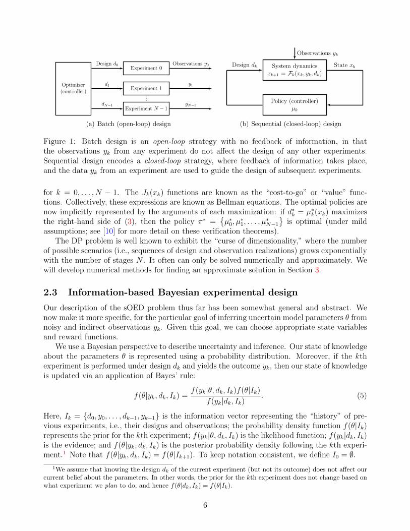
Design approaches that produce a policy are sequential (closed-loop) designs because theoutcomes of the previous experiments are necessary to determine the current state, whichin turn is needed to apply the policy. These approaches contrast with batch (open-loop)designs, where the designs are determined only from the initial state and do not dependon subsequent observations (hence, no feedback). Figure 1 illustrates these two differentstrategies.

4

• Observations: yk ∈ Yk. The observations from each experiment are endowed with un-certainties representing both measurement noise and modeling error. Along with prioruncertainty on the model parameters, these are assumed to be the only sources of uncer-tainty in the experimental campaign. Some models might also have internal stochasticdynamics, but we do not study such cases here. We consider continuous real-valuedobservations.

• Stage reward: gk(xk, yk, dk). The stage reward reflects the immediate reward associ-ated with performing a particular experiment. This quantity could depend on the state,observations, or design. Typically, it reflects the cost of performing the experiment (e.g.,money and/or time), as well as any additional benefits or penalties.

• Terminal reward: gN(xN). The terminal reward reflects the value of the final state xNthat is reached after all experiments have been completed.

• System dynamics: xk+1 = Fk(xk, yk, dk). The system dynamics describes the evolutionof the system state from one experiment to the next, and includes dependence on both thecurrent design and the observations resulting from the current experiment. This evolutionincludes the propagation of the belief state (e.g., statistical inference) and of the physicalstate. The specific form of the dynamics depends on the choice of state variable, and willbe discussed later.

Taking a decision-theoretic approach, we seek a design policy that maximizes the followingexpected utility (also called an expected reward) functional:

U(π) := Ey0,...,yN−1|π

[N−1∑k=0

gk (xk, yk, µk(xk)) + gN(xN)

], (1)

where the states must adhere to the system dynamics xk+1 = Fk(xk, yk, dk). The optimal policyis then

π∗ :={µ∗0, . . . , µ

∗N−1}

= arg maxπ={µ0,...,µN−1} U(π), (2)

s.t. xk+1 = Fk(xk, yk, dk),µk (Xk) ⊆ Dk, k = 0, . . . , N − 1.

For simplicity, we will refer to (2) as “the sOED problem.”

2.2 Dynamic programming form

The sOED problem involves the optimization of the expected reward functional (1) over a setof policy functions, which is a challenging problem to solve directly. Instead, we can expressthe problem in an equivalent form using Bellman’s principle of optimality [3, 4], leading to afinite-horizon dynamic programming formulation (e.g., [8, 9]):

Jk(xk) = maxdk∈Dk

Eyk|xk,dk [gk(xk, yk, dk) + Jk+1 (Fk(xk, yk, dk))] (3)

JN(xN) = gN(xN), (4)

5

Experiment 0

Experiment 1

...

Experiment N − 1

Optimizer(controller)

Observations y0

y1

yN−1

Design d0

d1

dN−1

(a) Batch (open-loop) design

System dynamicsxk+1 = Fk(xk, yk, dk)

Policy (controller)µk

State xkDesign dk

Observations yk

(b) Sequential (closed-loop) design

Figure 1: Batch design is an open-loop strategy with no feedback of information, in thatthe observations yk from any experiment do not affect the design of any other experiments.Sequential design encodes a closed-loop strategy, where feedback of information takes place,and the data yk from an experiment are used to guide the design of subsequent experiments.

for k = 0, . . . , N − 1. The Jk(xk) functions are known as the “cost-to-go” or “value” func-tions. Collectively, these expressions are known as Bellman equations. The optimal policies arenow implicitly represented by the arguments of each maximization: if d∗k = µ∗k(xk) maximizesthe right-hand side of (3), then the policy π∗ =

{µ∗0, µ

∗1, . . . , µ

∗N−1}

is optimal (under mildassumptions; see [10] for more detail on these verification theorems).

The DP problem is well known to exhibit the “curse of dimensionality,” where the numberof possible scenarios (i.e., sequences of design and observation realizations) grows exponentiallywith the number of stages N . It often can only be solved numerically and approximately. Wewill develop numerical methods for finding an approximate solution in Section 3.

2.3 Information-based Bayesian experimental design

Our description of the sOED problem thus far has been somewhat general and abstract. Wenow make it more specific, for the particular goal of inferring uncertain model parameters θ fromnoisy and indirect observations yk. Given this goal, we can choose appropriate state variablesand reward functions.

We use a Bayesian perspective to describe uncertainty and inference. Our state of knowledgeabout the parameters θ is represented using a probability distribution. Moreover, if the kthexperiment is performed under design dk and yields the outcome yk, then our state of knowledgeis updated via an application of Bayes’ rule:

f(θ|yk, dk, Ik) =f(yk|θ, dk, Ik)f(θ|Ik)

f(yk|dk, Ik). (5)

Here, Ik = {d0, y0, . . . , dk−1, yk−1} is the information vector representing the “history” of pre-vious experiments, i.e., their designs and observations; the probability density function f(θ|Ik)represents the prior for the kth experiment; f(yk|θ, dk, Ik) is the likelihood function; f(yk|dk, Ik)is the evidence; and f(θ|yk, dk, Ik) is the posterior probability density following the kth experi-ment.1 Note that f(θ|yk, dk, Ik) = f(θ|Ik+1). To keep notation consistent, we define I0 = ∅.

1We assume that knowing the design dk of the current experiment (but not its outcome) does not affect ourcurrent belief about the parameters. In other words, the prior for the kth experiment does not change based onwhat experiment we plan to do, and hence f(θ|dk, Ik) = f(θ|Ik).

6

In this Bayesian setting, the “belief state” that describes the state of uncertainty after kexperiments is simply the posterior distribution. How to represent this distribution, and thushow to define xk,b in a computation, is an important question. Options include: (i) seriesrepresentations (e.g., polynomial chaos expansions) of the posterior random variable θ|Ik itself;(ii) numerical discretizations of the posterior probability density function f(θ|Ik) or cumulativedistribution function F (θ|Ik); (iii) parameters of these distributions, if the priors and posteriorsall belong to a simple parametric family; or (iv) the prior f(θ|I0) at k = 0 plus the entire historyof designs and observations from all previous experiments. For example, if θ is a discreterandom variable that can take on only a finite number of distinct values, then it is naturalto define xk,b as the finite-dimensional vector specifying the probability mass function of θ.This is the approach most often taken in constructing partially observable Markov decisionprocesses (POMDP) [53, 51]. Since we are interested in continuous and possibly unbounded θ,an analogous perspective would yield in principle an infinite-dimensional belief state—unless,again, the posteriors belonged to a parametric family (for instance, in the case of conjugatepriors and likelihoods). In this paper, we will not restrict our attention to standard parametricfamilies of distributions, however, and thus we will employ finite-dimensional discretizations ofinfinite-dimensional belief states. The level of discretization is a refinable numerical parameter;details are deferred to Section 3.3. We will also use the shorthand xk,b = θ|Ik to convey theunderlying notion that the belief state is just the current posterior distribution.

Following the information-theoretic approach suggested by Lindley [40], we choose the ter-minal reward to be the Kullback-Leibler (KL) divergence from the final posterior (after all Nexperiments have been performed) to the prior (before any experiment has been performed):

gN(xN) = DKL

(fθ|IN || fθ|I0

)=

∫fθ|IN (θ) ln

[fθ|IN (θ)

fθ|I0(θ)

]dθ . (6)

The stage rewards {gk}k<N can then be chosen to reflect all other immediate rewards or costsassociated with performing particular experiments.

We use the KL divergence in our design objective (1) for several reasons. First, as shownin [29], the expected KL divergence belongs to a broad class of useful divergence measures ofthe information in a statistical experiment; this class of divergences is defined by a minimal setof requirements that must be satisfied to induce a total information ordering on the space ofpossible experiments.2 Interestingly, these requirements do not rely on a Bayesian perspectiveor a decision-theoretic formulation, though they can be interpreted quite naturally in thesesettings. Second, and perhaps more immediately, the KL divergence quantifies informationgain in the sense of Shannon information [20, 44]. A large KL divergence from posterior toprior implies that the observations yk decrease entropy in θ by a large amount, and hence thatthe observations are informative for parameter inference. Indeed, the expected KL divergenceis also equivalent to the mutual information between the parameters θ and the observations yk(treating both as random variables), given the design dk. Third, the KL divergence satisfiesuseful consistency conditions. It is invariant under one-to-one reparameterizations of θ. And

2As shown in Section 4.5 of [33], any reward function that introduces a non-trivial ordering on the space ofpossible experiments, according to the criteria formulated in [29], cannot be linear in the belief state. (Notethat this result precludes the use of non-centered posterior moments as reward functions.) Consequently, thecorresponding Bellman cost-to-go functions cannot be guaranteed to be piecewise linear and convex. Thoughmany state-of-the-art POMDP algorithms have been developed specifically for piecewise linear and convex costfunctions, they are generally not suitable for our sOED problem.

7

while it is directly applicable to non-Gaussian distributions and to forward models that arenonlinear in the parameters θ, maximizing KL divergence in the linear-Gaussian case reducesto Bayesian D-optimal design from linear optimal design theory [18] (i.e., maximizing thedeterminant of the posterior precision matrix, and hence of the Fisher information matrix plusthe prior precision). Finally we should note that, as an alternative to KL divergence, it isentirely reasonable to construct a terminal reward from some other loss function tied to analternative goal (e.g., squared error loss if the goal is point estimation). But in the absence ofsuch a goal, the KL divergence is a general-purpose objective that seeks to maximize learningabout the uncertain environment represented by θ, and should lead to good performance for abroad range of estimation tasks.

2.4 Notable suboptimal sequential design methods

Two design approaches frequently encountered in the OED literature are batch design andgreedy/myopic sequential design. Both can be seen as special cases or restrictions of the sOEDproblem formulated here, and are thus in general suboptimal. We illustrate these relationshipsbelow.

Batch OED involves the concurrent design of all experiments, and hence the outcome of anyexperiment cannot affect the design of the others. Mathematically, the policy functions µk forbatch design do not depend on the states xk, since no feedback is involved. (2) thus reduces toan optimization problem over the joint design space D := D0×D1× · · · DN−1 rather than overa space of policy functions, i.e.,

(d∗0, . . . , d

∗N−1)

= arg max(d0,...,dN−1)∈D

Ey0,...,yN−1|d0,...,dN−1

[N−1∑k=0

gk(xk, yk, dk) + gN(xN)

], (7)

subject to the system dynamics xk+1 = Fk(xk, yk, dk), for k = 0, . . . , N − 1. Since batch OEDinvolves the application of stricter constraints to the sOED problem than (2), it generally yieldssuboptimal designs.

Greedy design is a particular sequential and closed-loop formulation where only the nextexperiment is considered at each stage, without taking into account the entire horizon of futureexperiments and system dynamics.3 Mathematically, the greedy policy results from solving

Jk(xk) = maxdk∈Dk

Eyk|xk,dk [gk(xk, yk, dk)] , (8)

where the states must obey the system dynamics xk+1 = Fk(xk, yk, dk), k = 0, . . . , N − 1. Ifdgrk = µgr

k (xk) maximizes the right-hand side of (8) for all k = 0, . . . , N − 1, then the policyπgr =

{µgr0 , µ

gr1 , . . . , µ

grN−1}

is the greedy policy. Note that the terminal reward in (4) no longerplays a role in greedy design.4 Since greedy design involves truncating the DP form of thesOED problem, it again yields suboptimal designs.

3The greedy experimental design strategies considered in this paper are instances of greedy experimentaldesign with feedback. This is a different notion than greedy optimization of a batch experimental design problem,where no feedback of data occurs between experiments. The latter is simply a suboptimal solution strategy for(7), wherein the dk are chosen in sequence.

4An information-based greedy design for parameter inference would thus require moving the informationgain objective into the stage rewards gk, e.g., an incremental information gain formulation [56].

8

3 Numerical approaches

Approximate dynamic programming (ADP) broadly refers to numerical methods for findingan approximate solution to a DP problem. The development of such techniques has beenthe target of substantial research efforts across a number of communities (e.g., control theory,operations research, machine learning), targeting different variations of the DP problem. Whilea variety of terminologies are used in these fields, there is often a large overlap among thefundamental spirits of their solution approaches. We thus take a perspective that groups manyADP techniques into two broad categories:

1. Problem approximation: These are ADP techniques that do not provide a naturalway to refine the approximation, or where refinement does not lead to the solution of theoriginal problem. Such techniques typically lead to suboptimal strategies (e.g., batch andgreedy designs, certainty-equivalent control, Gaussian approximations).

2. Solution approximation: Here there is some natural way to refine the approximation,such that the effects of approximation diminish with refinement. These methods havesome notion of “convergence” and may be refined towards the solution of the originalproblem. Methods used in solution approximation include policy iteration, value functionand Q-factor approximations, numerical optimization, Monte Carlo sampling, regression,quadrature and numerical integration, discretization and aggregation, and rolling horizonprocedures.

In practice, techniques from both categories are often combined in order to find an approximatesolution to a DP problem. The approach in this paper will to try to preserve the originalproblem as much as possible, relying more heavily on solution approximation techniques toapproximately solve the exact problem.

Subsequent sections (Sections 3.1–3.3) will describe successive building blocks of our ADPapproach, and the entire algorithm will be summarized in Section 3.4.

3.1 Policy representation

In seeking the optimal policy, we first must be able to represent a (generally suboptimal)policy π = {µ0, µ1, . . . , µN−1}. One option is to represent a candidate policy function µk(xk)directly (and approximately)—for example, by brute-force tabulation over a finite collectionof xk values representing a discretization of the state space, or by using standard functionapproximation techniques. On the other hand, one can preserve the recursive structure of theBellman equations and “parameterize” the policy via approximations of the value functionsappearing in (3). We take this approach here. In particular, we represent the policy using onestep of lookahead [8], thus retaining some structure from the original DP problem while keepingthe method computationally feasible. By looking ahead only one step, the recursion betweenvalue functions is broken and the exponential growth of computational cost with respect to the

9

horizon N is reduced to linear growth.5 The one-step lookahead policy representation6 is:

µk(xk) = arg maxdk∈Dk

Eyk|xk,dk[gk(xk, yk, dk) + Jk+1 (Fk (xk, yk, dk))

], (9)

for k = 0, . . . , N − 1, and JN(xN) ≡ gN(xN). The policy function µk is therefore indirectly

represented via the approximate value function Jk+1, and one can view the policy π as implicitlyparameterized by the set of value functions J1, . . . , JN .7 If Jk+1(xk+1) = Jk+1(xk+1), we recoverthe Bellman equations (3) and (4), and hence we have µk = µ∗k. Therefore we would like to find

a collection of {Jk+1}k that is close to {Jk+1}k.We employ a simple parametric “linear architecture” for these value function approxima-

tions:

Jk(xk) = r>k φk(xk) =m∑i=1

rk,iφk,i(xk), (10)

where rk,i is the coefficient (weight) corresponding to the ith feature (basis function) φk,i(xk).While more sophisticated nonlinear or even nonparametric function approximations are possible(e.g., k-nearest-neighbor [30], kernel regression [48], neural networks [11]), the linear approxi-mator is easy to use and intuitive to understand [39], and is often required for many analysis

and convergence results [9]. It follows that the construction of Jk(xk) involves the selection offeatures and the training of coefficients.

The choice of features is an important but often difficult task. A concise set of featuresthat is relevant to the actual dependence of the value function on the state can substantiallyimprove the accuracy and efficiency of (10) and, in turn, of the overall algorithm. Identifyinghelpful features, however, is non-trivial. In the machine learning and statistics communities,substantial research has been dedicated to the development of systematic procedures for bothextracting and selecting features [31, 41]. Nonetheless, finding good features in practice oftenrelies on experience, trial and error, and expert knowledge of the particular problem at hand.We acknowledge the difficulty of this process, but do not pursue a detailed discussion of generaland systematic feature construction here. Instead, we employ a reasonable heuristic by choosingfeatures that are polynomial functions of the mean and log-variance of the belief state, as wellas of the physical state. The main motivation for this choice stems from the KL divergenceterm in the terminal reward. The impact of this terminal reward is propagated to earlier stagesvia the value functions, and hence the value functions must represent the state-dependenceof future information gain. While the belief state is generally not Gaussian and the optimalpolicy is expected to depend on higher moments, the analytic expression for the KL divergence

5Multi-step lookahead is possible in theory, but impractical, as the amount of online computation would beintractable given continuous state and design spaces.

6It is crucial to note that “one-step lookahead” is not greedy design, since future effects are still included(within the term Jk+1). The name simply describes the structure of the policy representation, indicating that

approximation is made after one step of looking ahead (i.e., in Jk+1).7A similar method is the use of Q-factors [62, 63]: µk(xk) = arg maxdk∈Dk

Qk(xk, dk), where the Q-factorcorresponding to the optimal policy is Qk(xk, dk) ≡ Eyk|xk,dk

[gk(xk, yk, dk) + Jk+1 (Fk(xk, yk, dk))]. The func-

tions Qk(xk, dk) have a higher input dimension than Jk(xk), but once they are available, the correspondingpolicy can be applied without evaluating the system dynamics Fk, and is thus known as a “model-free” method.Q-learning via value iteration is a prominent method in reinforcement learning.

10

between two univariate Gaussian distributions, which involves their mean and log-varianceterms, provides a starting point for promising features. Polynomials then generalize this initialset. We will provide more detail about our feature choices in Section 4. For the presentpurpose of developing our ADP method, we assume that the features are fixed. We now focuson developing an efficient procedure for training the coefficients.

3.2 Policy construction via approximate value iteration

Having decided on a way to represent candidate policies, we now aim to construct policieswithin this representation class that are close to the optimal policy. We achieve this goal byconstructing and iteratively refining value function approximations via regression over targetedrelevant states.

Note that the procedure for policy construction described in this section can be performedentirely offline. Once this process is terminated and the resulting value function approximationsare available, applying the policy as experimental data are acquired is an online process, whichinvolves evaluating (9). The computational costs of these online evaluations are generally muchsmaller than those of offline policy construction.

3.2.1 Backward induction with regression

Our goal is to find value function approximations (implicitly, policy parameterizations) Jk thatare close to the value functions Jk of the optimal policy, i.e., the value functions that satisfy (3)and (4). We take a direct approach, and would in principle like to solve the following “ideal”regression problem: minimize the squared error of the approximation under the state measureinduced by the optimal policy,

minrk,∀k

∫X1×···×XN−1

[N−1∑k=1

(Jk(xk)− r>k φk(xk)

)2]fπ∗(x1, . . . , xN−1) dx1 . . . dxN−1. (11)

The weighted L2 norm above is also known as the D-norm in other work [57]; its associateddensity function is denoted by fπ∗(x1, . . . , xN−1). Here we have imposed the linear architecture

Jk(xk) = r>k φk(xk) (10). Xk is the support of xk.In practice, the integral above must be replaced by a sum over discrete regression points, and

the distribution of these points reflects where we place more emphasis on the approximationbeing accurate. Intuitively, we would like more accurate approximations in regions of thestate space that are more frequently visited under the optimal policy, e.g., as captured bysampling from fπ∗ . But we should actually consider a further desideratum: accuracy over thestate measure induced by the optimal policy and by the numerical methods used to evaluatethis policy (whatever they may be). Numerical optimization methods used to solve (9), forinstance, may visit many intermediate values of dk and hence of xk+1 = Fk (xk, yk, dk). Theaccuracy of the value function approximation at these intermediate states can be crucial; poorapproximations can potentially mislead the optimizer to arrive at completely different designs,and in turn change the outcomes of regression and policy evaluation. We thus include thestates visited within our numerical methods (such as iterations of stochastic approximation forsolving (9)) as regression points too. For simplicity of notation, we henceforth let fπ∗ representthe state measure induced by the optimal policy and the associated numerical methods.

11

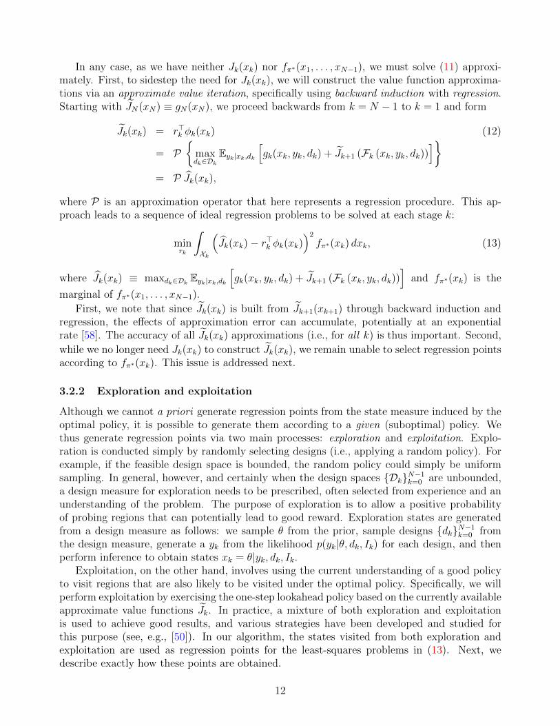
In any case, as we have neither Jk(xk) nor fπ∗(x1, . . . , xN−1), we must solve (11) approxi-mately. First, to sidestep the need for Jk(xk), we will construct the value function approxima-tions via an approximate value iteration, specifically using backward induction with regression.Starting with JN(xN) ≡ gN(xN), we proceed backwards from k = N − 1 to k = 1 and form

Jk(xk) = r>k φk(xk) (12)

= P{

maxdk∈Dk

Eyk|xk,dk[gk(xk, yk, dk) + Jk+1 (Fk (xk, yk, dk))

]}= P Jk(xk),

where P is an approximation operator that here represents a regression procedure. This ap-proach leads to a sequence of ideal regression problems to be solved at each stage k:

minrk

∫Xk

(Jk(xk)− r>k φk(xk)

)2fπ∗(xk) dxk, (13)

where Jk(xk) ≡ maxdk∈Dk Eyk|xk,dk[gk(xk, yk, dk) + Jk+1 (Fk (xk, yk, dk))

]and fπ∗(xk) is the

marginal of fπ∗(x1, . . . , xN−1).

First, we note that since Jk(xk) is built from Jk+1(xk+1) through backward induction andregression, the effects of approximation error can accumulate, potentially at an exponentialrate [58]. The accuracy of all Jk(xk) approximations (i.e., for all k) is thus important. Second,

while we no longer need Jk(xk) to construct Jk(xk), we remain unable to select regression pointsaccording to fπ∗(xk). This issue is addressed next.

3.2.2 Exploration and exploitation

Although we cannot a priori generate regression points from the state measure induced by theoptimal policy, it is possible to generate them according to a given (suboptimal) policy. Wethus generate regression points via two main processes: exploration and exploitation. Explo-ration is conducted simply by randomly selecting designs (i.e., applying a random policy). Forexample, if the feasible design space is bounded, the random policy could simply be uniformsampling. In general, however, and certainly when the design spaces {Dk}N−1k=0 are unbounded,a design measure for exploration needs to be prescribed, often selected from experience and anunderstanding of the problem. The purpose of exploration is to allow a positive probabilityof probing regions that can potentially lead to good reward. Exploration states are generatedfrom a design measure as follows: we sample θ from the prior, sample designs {dk}N−1k=0 fromthe design measure, generate a yk from the likelihood p(yk|θ, dk, Ik) for each design, and thenperform inference to obtain states xk = θ|yk, dk, Ik.

Exploitation, on the other hand, involves using the current understanding of a good policyto visit regions that are also likely to be visited under the optimal policy. Specifically, we willperform exploitation by exercising the one-step lookahead policy based on the currently availableapproximate value functions Jk. In practice, a mixture of both exploration and exploitationis used to achieve good results, and various strategies have been developed and studied forthis purpose (see, e.g., [50]). In our algorithm, the states visited from both exploration andexploitation are used as regression points for the least-squares problems in (13). Next, wedescribe exactly how these points are obtained.

12

3.2.3 Iteratively updating approximations of the optimal policy

Exploitation in the present context involves a dilemma of sorts: generating exploitation pointsfor regression requires the availability of an approximate optimal policy, but the constructionof such a policy requires regression points. To address this issue, we introduce an iterativeapproach to update the approximation of the optimal policy and the state measure inducedby it. We refer to this mechanism as “policy update” in this paper, to avoid confusion withapproximate value iteration introduced previously.

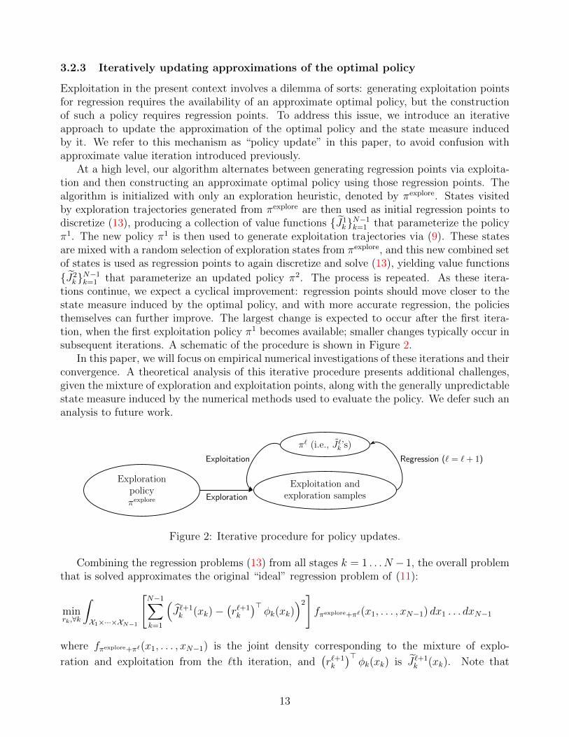
At a high level, our algorithm alternates between generating regression points via exploita-tion and then constructing an approximate optimal policy using those regression points. Thealgorithm is initialized with only an exploration heuristic, denoted by πexplore. States visitedby exploration trajectories generated from πexplore are then used as initial regression points todiscretize (13), producing a collection of value functions {J1

k}N−1k=1 that parameterize the policyπ1. The new policy π1 is then used to generate exploitation trajectories via (9). These statesare mixed with a random selection of exploration states from πexplore, and this new combined setof states is used as regression points to again discretize and solve (13), yielding value functions

{J2k}N−1k=1 that parameterize an updated policy π2. The process is repeated. As these itera-

tions continue, we expect a cyclical improvement: regression points should move closer to thestate measure induced by the optimal policy, and with more accurate regression, the policiesthemselves can further improve. The largest change is expected to occur after the first itera-tion, when the first exploitation policy π1 becomes available; smaller changes typically occur insubsequent iterations. A schematic of the procedure is shown in Figure 2.

In this paper, we will focus on empirical numerical investigations of these iterations and theirconvergence. A theoretical analysis of this iterative procedure presents additional challenges,given the mixture of exploration and exploitation points, along with the generally unpredictablestate measure induced by the numerical methods used to evaluate the policy. We defer such ananalysis to future work.

π` (i.e., J `k’s)

Exploitation andexploration samples

Explorationpolicyπexplore Exploration

Exploitation Regression (` = `+ 1)

Figure 2: Iterative procedure for policy updates.

Combining the regression problems (13) from all stages k = 1 . . . N − 1, the overall problemthat is solved approximates the original “ideal” regression problem of (11):

minrk,∀k

∫X1×···×XN−1

[N−1∑k=1

(J `+1k (xk)−

(r`+1k

)>φk(xk)

)2]fπexplore+π`(x1, . . . , xN−1) dx1 . . . dxN−1

where fπexplore+π`(x1, . . . , xN−1) is the joint density corresponding to the mixture of explo-

ration and exploitation from the `th iteration, and(r`+1k

)>φk(xk) is J `+1

k (xk). Note that

13

fπexplore+π`(x1, . . . , xN−1) lags one iteration behind J `+1k (xk) and J `+1

k (xk), since we need tohave constructed the policy before we can sample trajectories from it.

Simulating exploitation trajectories, evaluating policies, and computing the values of J forthe purpose of linear regression all involve maximizing an expectation over a continuous designspace (see both (9) and the definition of J following (13)). While the expected value generallycannot be found analytically, a robust and natural approximation may be obtained via MonteCarlo estimation. As a result, the optimization objective is effectively noisy. We use Robbins-Monro (or Kiefer-Wolfowitz if gradients are not available analytically) stochastic approximationalgorithms to solve these stochastic optimization problems; more details can be found in [35].

3.3 Belief state representation

As discussed in Section 2.3, a natural choice of the belief state xk,b in the present context is theposterior θ|Ik. An important question is how to represent this belief state numerically. Thereare two major considerations. First, since we seek to accommodate general nonlinear forwardmodels with continuous parameters, the posterior distributions are continuous, non-Gaussian,and not from any particular parametric family; such distributions are difficult to represent in afinite- or low-dimensional manner. Second, sequential Bayesian inference, as part of the systemdynamics Fk, needs to be performed repeatedly under different realizations of dk, yk, and xk.

In this paper, we represent belief states numerically by discretizing their probability densityfunctions on a dynamically evolving grid. To perform Bayesian inference, the grid needs to beadapted in order to ensure reasonable coverage and resolution of the posterior density. Ourscheme first computes values of the unnormalized posterior density on the current grid, andthen decides whether grid expansion is needed on either side, based on a threshold for the ratioof the density value at the grid endpoints to the value of the density at the mode. Second,a uniform grid is laid over the expanded regions, and new unnormalized posterior densityvalues are computed. Finally, a new grid encompassing the original and expanded regions isconstructed such that the probability masses between neighboring grid points are equal; thisprovides a mechanism for coarsening the grid in regions of low probability density.

While this adaptive gridding approach is suitable for one- or perhaps two-dimensional θ,it becomes impractical in higher dimensions. In a companion paper, we will introduce a moreflexible technique based on transport maps (e.g., [59, 45]) that can represent multi-dimensionalnon-Gaussian posteriors in a scalable way, and that immediately enables fast Bayesian inferencefrom multiple realizations of the data.

3.4 Algorithm pseudocode

The complete approximate dynamic programming approach developed over the preceding sec-tions is outlined in Algorithm 1.

4 Numerical examples

We present two examples to highlight different aspects of the approximate dynamic program-ming methods developed in this paper. First is a linear-Gaussian problem (Section 4.1). Thisexample establishes (a) the ability of our numerical methods to solve an sOED problem, in

14

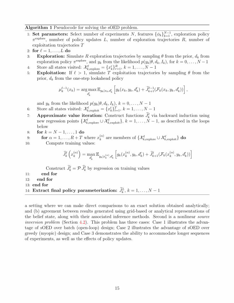
Algorithm 1 Pseudocode for solving the sOED problem.

1: Set parameters: Select number of experiments N , features {φk}N−1k=1 , exploration policyπexplore, number of policy updates L, number of exploration trajectories R, number ofexploitation trajectories T

2: for ` = 1, . . . , L do3: Exploration: Simulate R exploration trajectories by sampling θ from the prior, dk from

exploration policy πexplore, and yk from the likelihood p(yk|θ, dk, Ik), for k = 0, . . . , N − 14: Store all states visited: X `

k,explore = {xrk}Rr=1, k = 1, . . . , N − 15: Exploitation: If ` > 1, simulate T exploitation trajectories by sampling θ from the

prior, dk from the one-step lookahead policy

µ`−1k (xk) = arg maxd′k

Eyk|xk,d′k[gk(xk, yk, d

′k) + J `−1k+1(Fk(xk, yk, d′k))

],

and yk from the likelihood p(yk|θ, dk, Ik), k = 0, . . . , N − 16: Store all states visited: X `

k,exploit = {xtk}Tt=1, k = 1, . . . , N − 1

7: Approximate value iteration: Construct functions J `k via backward induction usingnew regression points {X `

k,explore ∪ X `k,exploit}, k = 1, . . . , N − 1, as described in the loops

below8: for k = N − 1, . . . , 1 do9: for α = 1, . . . , R + T where x

(α)k are members of {X `

k,explore ∪ X `k,exploit} do

10: Compute training values:

J `k

(x(α)k

)= max

d′k

Eyk|x(α)k ,d′k

[gk(x

(α)k , yk, d

′k) + J `k+1(Fk(x(α)k , yk, d

′k))]

Construct J `k = P J `k by regression on training values11: end for12: end for13: end for14: Extract final policy parameterization: JLk , k = 1, . . . , N − 1

a setting where we can make direct comparisons to an exact solution obtained analytically;and (b) agreement between results generated using grid-based or analytical representations ofthe belief state, along with their associated inference methods. Second is a nonlinear sourceinversion problem (Section 4.2). This problem has three cases: Case 1 illustrates the advan-tage of sOED over batch (open-loop) design; Case 2 illustrates the advantage of sOED overgreedy (myopic) design; and Case 3 demonstrates the ability to accommodate longer sequencesof experiments, as well as the effects of policy updates.

15

4.1 Linear-Gaussian problem

4.1.1 Problem setup

Consider a forward model that is linear in its parameters θ, with a scalar output corrupted byadditive Gaussian noise ε ∼ N (0, σ2

ε ):

yk = G(θ, dk) + ε = θdk + ε. (14)

The prior on θ is N (s0, σ20) and the design parameter is d ∈ [dL, dR]. The resulting infer-

ence problem on θ has a conjugate Gaussian structure, such that all subsequent posteriors areGaussian with mean and variance given by

(sk+1, σ

2k+1

)=

yk/dkσ2ε /d

2k

+ skσ2k

1σ2ε /d

2k

+ 1σ2k

,1

1σ2ε /d

2k

+ 1σ2k

. (15)

Let us consider the design of N = 2 experiments, with prior parameters s0 = 0 and σ20 = 9,

noise variance σ2ε = 1, and design limits dL = 0.1 and dR = 3. The Gaussian posteriors in this

problem—i.e., the belief states—are completely specified by values of the mean and variance;hence we may designate xk,b = (sk, σ

2k). We call this parametric representation the “analytical

method,” as it also allows inference to be performed exactly using (15). The analytical methodwill be compared to the adaptive-grid representation of the belief state (along with its associatedinference procedure) described in Section 3.3. In this example, the adaptive grids use 50 nodes.There is no physical state xk,p; we simply have xk = xk,b.

Our goal is to infer θ. The stage and terminal reward functions are:

gk(xk, yk, dk) = 0, k ∈ {0, 1}gN(xN) = DKL

(fθ|IN || fθ|I0

)− 2

(lnσ2

N − ln 2)2.

The terminal reward is thus a combination of information gain in θ and a penalty for deviationfrom a particular log-variance target. The latter term increases the difficulty of this problem bymoving the outputs of the optimal policy away from the design space boundary; doing so helpsavoid the fortuitous construction of successful policies.8 Following the discussion in Section 3.1,we approximate the value functions using features φk,i (in (10)) that are polynomials of degreetwo or less in the posterior mean and log-variance: 1, sk, ln(σ2

k), s2k, ln2(σ2

k), and sk ln(σ2k).

When using the grid representation of the belief state, the values of the features are evaluatedby trapezoidal integration rule. The terminal KL divergence is approximated by first estimatingthe mean and variance, and then applying the analytical formula for KL divergence betweenGaussians. The ADP approach uses L = 3 policy updates (described in Section 3.2.3); theseupdates are conducted using regression points that, for the first iteration (` = 1), are generatedentirely via exploration. The design measure for exploration is chosen to be dk ∼ N (1.25, 0.52)in order to have a wide coverage of the design space.9 Subsequent iterations use regression with

8Without the second term in the terminal reward, the optimal policies will always be those that lead to thehighest achievable signal, which occurs at the dk = 3 boundary. Policies that produce such boundary designscan be realized even when the overall value function approximation is poor. Nothing is wrong with this situationper se, but adding the second term leads to a more challenging test of the numerical approach.

9Designs proposed outside the design constraints are simply projected back to the nearest feasible design;thus the actual design measure is not exactly Gaussian.

16

a mix of 30% exploration samples and 70% exploitation samples. At each iteration, we use 1000regression points for the analytical method and 500 regression points for the grid method.

To compare the policies generated via different numerical methods, we apply each policyto generate 1000 simulated trajectories. Producing a trajectory of the system involves firstsampling θ from its prior, applying the policy on the inital belief state x0 to obtain the firstdesign d0, drawing a sample y0 to simulate the outcome of the first experiment, updating thebelief state to x1 = θ|y0, d0, I0, applying the policy to x1 in order to obtain d1, and so on.The mean reward over all these trajectories is an estimate of the expected total reward (1).But evaluating the reward requires some care. Our procedure for doing so is summarizedin Algorithm 2. Each policy is first applied to belief state trajectories computed using thesame state representation (i.e., analytical or grid) originally used to construct that policy; thisyields sequences of designs and observations. Then, to assess the reward from each trajectory,inference is performed on the associated sequence of designs and observations using a commonassessment framework—the analytical method in this case—regardless of how the trajectorywas produced. This process ensures a fair comparison between policies, where the designsare produced using the “native” belief state representation for which the policy was originallycreated, but all final trajectories are assessed using a common method.

Algorithm 2 Procedure for assessing policies by simulating trajectories.

1: Select a “native” belief state representation to generate policy (e.g., analytical orgrid)

2: Construct policy π using this belief state representation3: for q = 1, . . . , ntrajectories do4: Apply policy using the native belief state representation: Sample θ from the prior.

Then evaluate dk by applying the constructed policy µk(xk), sample yk from the likelihoodp(yk|θ, dk, Ik) to simulate the experimental outcome, and evaluate xk+1 = Fk(xk, yk, dk),for k = 0, . . . , N − 1.

5: Evaluate rewards via a common assessment framework: Discard the belief statesequence {xk}k. Perform inference on the {dk}k and {yk}k sequences from the currenttrajectory and evaluate the total reward using a chosen common assessment framework.

6: end for

4.1.2 Results

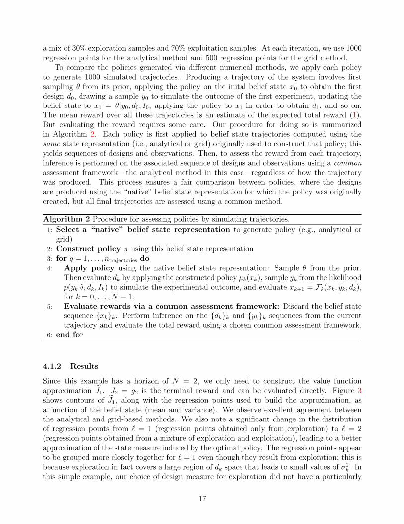
Since this example has a horizon of N = 2, we only need to construct the value functionapproximation J1. J2 = g2 is the terminal reward and can be evaluated directly. Figure 3shows contours of J1, along with the regression points used to build the approximation, asa function of the belief state (mean and variance). We observe excellent agreement betweenthe analytical and grid-based methods. We also note a significant change in the distributionof regression points from ` = 1 (regression points obtained only from exploration) to ` = 2(regression points obtained from a mixture of exploration and exploitation), leading to a betterapproximation of the state measure induced by the optimal policy. The regression points appearto be grouped more closely together for ` = 1 even though they result from exploration; this isbecause exploration in fact covers a large region of dk space that leads to small values of σ2

k. Inthis simple example, our choice of design measure for exploration did not have a particularly

17

negative impact on the expected reward for ` = 1 (see Figure 5). However, this situation caneasily change for problems with more complicated value functions and less suitable choices ofthe exploration policy.

−10 −5 0 5 100

3

6

9

s1

σ2 1

−25

−15

−5

5

−10 −5 0 5 100

3

6

9

s1σ2 1

−25

−15

−5

5

−10 −5 0 5 100

3

6

9

s1

σ2 1

−25

−15

−5

5

(a) Analytical method

−10 −5 0 5 100

3

6

9

s1

σ2 1

−25

−15

−5

5

−10 −5 0 5 100

3

6

9

s1

σ2 1

−25

−15

−5

5

−10 −5 0 5 100

3

6

9

s1

σ2 1

−25

−15

−5

5

(b) Grid method

Figure 3: Linear-Gaussian problem: contours represent J1(x1) and blue points are the regressionpoints used to build these value function approximations. The left, middle, and right columnscorrespond to ` = 1, 2, and 3, respectively.

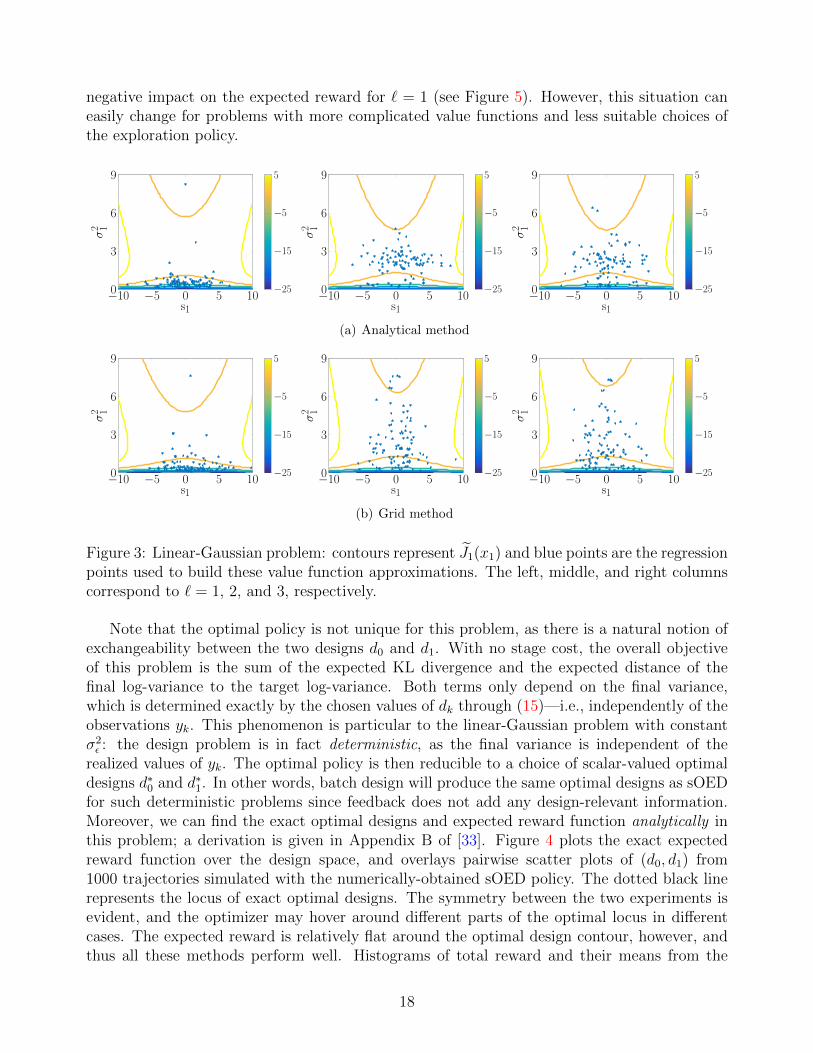
Note that the optimal policy is not unique for this problem, as there is a natural notion ofexchangeability between the two designs d0 and d1. With no stage cost, the overall objectiveof this problem is the sum of the expected KL divergence and the expected distance of thefinal log-variance to the target log-variance. Both terms only depend on the final variance,which is determined exactly by the chosen values of dk through (15)—i.e., independently of theobservations yk. This phenomenon is particular to the linear-Gaussian problem with constantσ2ε : the design problem is in fact deterministic, as the final variance is independent of the

realized values of yk. The optimal policy is then reducible to a choice of scalar-valued optimaldesigns d∗0 and d∗1. In other words, batch design will produce the same optimal designs as sOEDfor such deterministic problems since feedback does not add any design-relevant information.Moreover, we can find the exact optimal designs and expected reward function analytically inthis problem; a derivation is given in Appendix B of [33]. Figure 4 plots the exact expectedreward function over the design space, and overlays pairwise scatter plots of (d0, d1) from1000 trajectories simulated with the numerically-obtained sOED policy. The dotted black linerepresents the locus of exact optimal designs. The symmetry between the two experiments isevident, and the optimizer may hover around different parts of the optimal locus in differentcases. The expected reward is relatively flat around the optimal design contour, however, andthus all these methods perform well. Histograms of total reward and their means from the

18

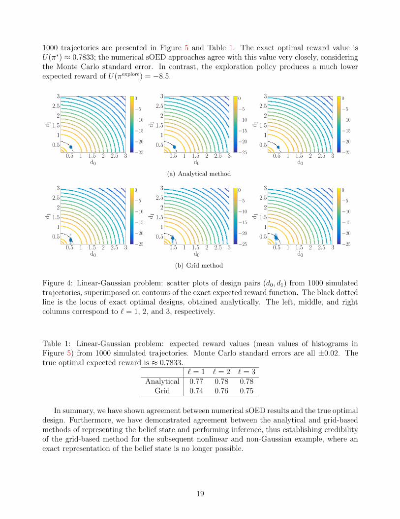
1000 trajectories are presented in Figure 5 and Table 1. The exact optimal reward value isU(π∗) ≈ 0.7833; the numerical sOED approaches agree with this value very closely, consideringthe Monte Carlo standard error. In contrast, the exploration policy produces a much lowerexpected reward of U(πexplore) = −8.5.

0.5 1 1.5 2 2.5 3

0.5

1

1.5

2

2.5

3

d0

d1

−25

−20

−15

−10

−5

0

0.5 1 1.5 2 2.5 3

0.5

1

1.5

2

2.5

3

d0

d1

−25

−20

−15

−10

−5

0

0.5 1 1.5 2 2.5 3

0.5

1

1.5

2

2.5

3

d0

d1

−25

−20

−15

−10

−5

0

(a) Analytical method

0.5 1 1.5 2 2.5 3

0.5

1

1.5

2

2.5

3

d0

d1

−25

−20

−15

−10

−5

0

0.5 1 1.5 2 2.5 3

0.5

1

1.5

2

2.5

3

d0

d1

−25

−20

−15

−10

−5

0

0.5 1 1.5 2 2.5 3

0.5

1

1.5

2

2.5

3

d0d1

−25

−20

−15

−10

−5

0

(b) Grid method

Figure 4: Linear-Gaussian problem: scatter plots of design pairs (d0, d1) from 1000 simulatedtrajectories, superimposed on contours of the exact expected reward function. The black dottedline is the locus of exact optimal designs, obtained analytically. The left, middle, and rightcolumns correspond to ` = 1, 2, and 3, respectively.

Table 1: Linear-Gaussian problem: expected reward values (mean values of histograms inFigure 5) from 1000 simulated trajectories. Monte Carlo standard errors are all ±0.02. Thetrue optimal expected reward is ≈ 0.7833.

` = 1 ` = 2 ` = 3Analytical 0.77 0.78 0.78

Grid 0.74 0.76 0.75

In summary, we have shown agreement between numerical sOED results and the true optimaldesign. Furthermore, we have demonstrated agreement between the analytical and grid-basedmethods of representing the belief state and performing inference, thus establishing credibilityof the grid-based method for the subsequent nonlinear and non-Gaussian example, where anexact representation of the belief state is no longer possible.

19

0 1 2 3 40

100

200

300

400

500

Reward

Count

mean = 0.77 ± 0.02

0 1 2 3 40

100

200

300

400

500

Reward

Count

mean = 0.78 ± 0.02

0 1 2 3 40

100

200

300

400

500

Reward

Count

mean = 0.78 ± 0.02

(a) Analytical method

0 1 2 3 40

100

200

300

400

500

Reward

Count

mean = 0.74 ± 0.02

0 1 2 3 40

100

200

300

400

500

Reward

Count

mean = 0.76 ± 0.02

0 1 2 3 40

100

200

300

400

500

Reward

Count

mean = 0.75 ± 0.02

(b) Grid method

Figure 5: Linear-Gaussian problem: total reward histograms from 1000 simulated trajectories.The left, middle, and right columns correspond to ` = 1, 2, and 3, respectively.

4.2 Contaminant source inversion problem

Consider a situation where a chemical contaminant is accidentally released into the air. Thecontaminant plume diffuses and is advected by the wind. It is crucial to infer the location of thecontaminant source so that an appropriate response can be undertaken. Suppose that an aerialor ground-based vehicle is dispatched to measure contaminant concentrations at a sequence ofdifferent locations, under a fixed time schedule. We seek the optimal policy for deciding wherethe vehicle should take measurements in order to maximize expected information gain in thesource location. Our sOED problem will also account for hard constraints on possible vehiclemovements, as well movement costs incorporated into the stage rewards.

We use the following simple plume model of the contaminant concentration at location zand time t, given source location θ:

G(θ, z, t) =s√

2π(√

1.2 + 4Dt) exp

(−‖ θ + dw(t)− z ‖2

2(1.2 + 4Dt)

), (16)

where s, D, and dw(t) are the known source intensity, diffusion coefficient, and cumulative netdisplacement due to wind up to time t, respectively. The displacement dw(t) depends on thetime history of the wind velocity. (Values of these coefficients will be specified later.) A totalof N measurements are performed, at uniformly spaced times given by t = k+ 1. (While t is acontinuous variable, we assume it to be suitably scaled so that it corresponds to the experimentindex in this fashion; hence, observation y0 is taken at t = 1, y1 at t = 2, etc.) The state xk is a

20

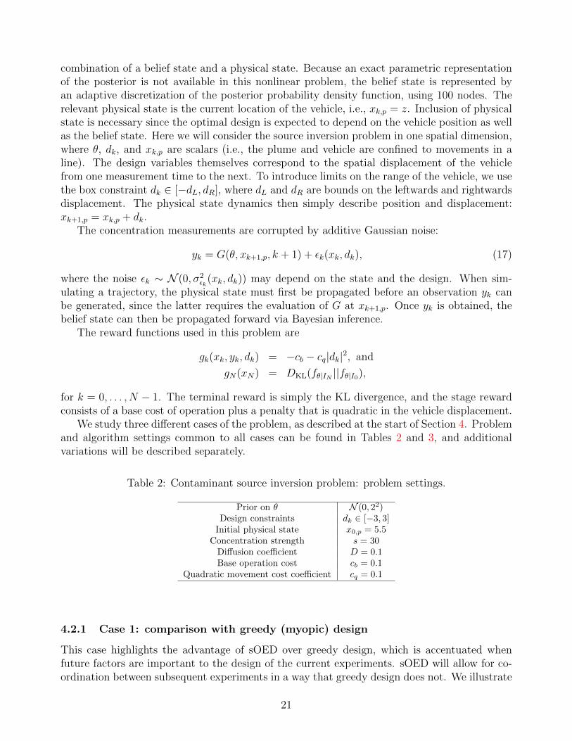
combination of a belief state and a physical state. Because an exact parametric representationof the posterior is not available in this nonlinear problem, the belief state is represented byan adaptive discretization of the posterior probability density function, using 100 nodes. Therelevant physical state is the current location of the vehicle, i.e., xk,p = z. Inclusion of physicalstate is necessary since the optimal design is expected to depend on the vehicle position as wellas the belief state. Here we will consider the source inversion problem in one spatial dimension,where θ, dk, and xk,p are scalars (i.e., the plume and vehicle are confined to movements in aline). The design variables themselves correspond to the spatial displacement of the vehiclefrom one measurement time to the next. To introduce limits on the range of the vehicle, we usethe box constraint dk ∈ [−dL, dR], where dL and dR are bounds on the leftwards and rightwardsdisplacement. The physical state dynamics then simply describe position and displacement:xk+1,p = xk,p + dk.

The concentration measurements are corrupted by additive Gaussian noise:

yk = G(θ, xk+1,p, k + 1) + εk(xk, dk), (17)

where the noise εk ∼ N (0, σ2εk

(xk, dk)) may depend on the state and the design. When sim-ulating a trajectory, the physical state must first be propagated before an observation yk canbe generated, since the latter requires the evaluation of G at xk+1,p. Once yk is obtained, thebelief state can then be propagated forward via Bayesian inference.

The reward functions used in this problem are

gk(xk, yk, dk) = −cb − cq|dk|2, and

gN(xN) = DKL(fθ|IN ||fθ|I0),

for k = 0, . . . , N − 1. The terminal reward is simply the KL divergence, and the stage rewardconsists of a base cost of operation plus a penalty that is quadratic in the vehicle displacement.

We study three different cases of the problem, as described at the start of Section 4. Problemand algorithm settings common to all cases can be found in Tables 2 and 3, and additionalvariations will be described separately.

Table 2: Contaminant source inversion problem: problem settings.

Prior on θ N (0, 22)Design constraints dk ∈ [−3, 3]

Initial physical state x0,p = 5.5Concentration strength s = 30

Diffusion coefficient D = 0.1Base operation cost cb = 0.1

Quadratic movement cost coefficient cq = 0.1

4.2.1 Case 1: comparison with greedy (myopic) design

This case highlights the advantage of sOED over greedy design, which is accentuated whenfuture factors are important to the design of the current experiments. sOED will allow for co-ordination between subsequent experiments in a way that greedy design does not. We illustrate

21

Table 3: Contaminant source inversion problem: algorithm settings.

Number of grid points 100Design measure for exploration policy dk ∼ N (0, 22)

Total number of regression points 500% of regression points from exploration 30%

Maximum number of optimization iterations 50Monte Carlo sample size in stochastic optimization 100

this idea via the wind factor: the air is calm initially, and then a constant wind of velocity 10commences at t = 1, leading to the following net displacement due to the wind up to time t:

dw(t) =

{0, t < 1

10(t− 1), t ≥ 1. (18)

Consider N = 2 experiments. Greedy design, by construction, chooses the first design to yieldthe single best experiment at t = 1. This experiment is performed before plume has beenadvected. sOED, along with batch design, can take advantage of the fact that the plume willhave moved by the second experiment, and make use of this knowledge even when designingthe first experiment.

Details of the problem setup and numerical solution are as follows. The observation noisevariance is set to σ2

εk= 4 for all experiments. Features for the representation of the value

function are analogous to those used in the previous example but now include the physical stateas well: that is, we use polynomials up to total degree two in the posterior mean, posteriorlog-variance, and physical state (including cross-terms). Posterior moments are evaluated bytrapezoidal rule integration on the adaptive grid. The terminal KL divergence is approximatedby first estimating the mean and variance, and then applying the analytical formula for KLdivergence between the associated Gaussian approximations. sOED uses L = 3 policy updates,with a design measure for exploration of dk ∼ N (0, 22). Policies are compared by applyingeach to 1000 simulated trajectories, as summarized in Algorithm 2. The common assessmentframework for this problem is a high-resolution grid discretization of the posterior probabilitydensity function with 1000 nodes.

Before presenting the results, we first provide some intuition for the progression of a singleexample trajectory, as shown in Figure 6. Suppose that a true value θ∗ of the source location hasbeen fixed (or sampled from the prior). The horizontal axis of the left figure corresponds to thephysical space, with the vehicle starting at the location marked by the black square. To performthe first experiment, the vehicle moves to a new location and acquires the noisy observationindicated by the blue cross, with the solid blue curve indicating the plume profile G(θ∗, z, t = 1)at that time. For the second experiment, the vehicle moves to another location and acquiresthe noisy observation indicated by the red cross; the dotted red curve shows the plume profileG(θ∗, z, t = 2), which has diffused slightly and been carried to the right by the wind. Theright figure shows the corresponding belief state (i.e., posterior density) at each stage. Startingfrom the solid blue prior density, the posterior density after the first experiment (dashed red)narrows only slightly, since the first observation is in a region dominated by measurement noise.The posterior after both experiments (dotted yellow), however, becomes much narrower, as thesecond observation is in a high-gradient region of the concentration profile and thus carries

22

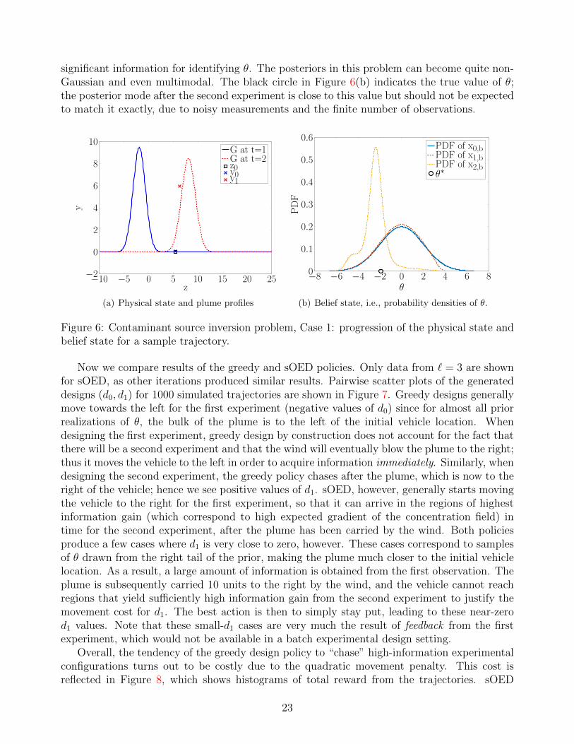
significant information for identifying θ. The posteriors in this problem can become quite non-Gaussian and even multimodal. The black circle in Figure 6(b) indicates the true value of θ;the posterior mode after the second experiment is close to this value but should not be expectedto match it exactly, due to noisy measurements and the finite number of observations.

−10 −5 0 5 10 15 20 25−2

0

2

4

6

8

10

z

y

G at t=1G at t=2z0y0y1

(a) Physical state and plume profiles

−8 −6 −4 −2 0 2 4 6 80

0.1

0.2

0.3

0.4

0.5

0.6

θPDF

PDF of x0,bPDF of x1,bPDF of x2,bθ∗

(b) Belief state, i.e., probability densities of θ.

Figure 6: Contaminant source inversion problem, Case 1: progression of the physical state andbelief state for a sample trajectory.

Now we compare results of the greedy and sOED policies. Only data from ` = 3 are shownfor sOED, as other iterations produced similar results. Pairwise scatter plots of the generateddesigns (d0, d1) for 1000 simulated trajectories are shown in Figure 7. Greedy designs generallymove towards the left for the first experiment (negative values of d0) since for almost all priorrealizations of θ, the bulk of the plume is to the left of the initial vehicle location. Whendesigning the first experiment, greedy design by construction does not account for the fact thatthere will be a second experiment and that the wind will eventually blow the plume to the right;thus it moves the vehicle to the left in order to acquire information immediately. Similarly, whendesigning the second experiment, the greedy policy chases after the plume, which is now to theright of the vehicle; hence we see positive values of d1. sOED, however, generally starts movingthe vehicle to the right for the first experiment, so that it can arrive in the regions of highestinformation gain (which correspond to high expected gradient of the concentration field) intime for the second experiment, after the plume has been carried by the wind. Both policiesproduce a few cases where d1 is very close to zero, however. These cases correspond to samplesof θ drawn from the right tail of the prior, making the plume much closer to the initial vehiclelocation. As a result, a large amount of information is obtained from the first observation. Theplume is subsequently carried 10 units to the right by the wind, and the vehicle cannot reachregions that yield sufficiently high information gain from the second experiment to justify themovement cost for d1. The best action is then to simply stay put, leading to these near-zerod1 values. Note that these small-d1 cases are very much the result of feedback from the firstexperiment, which would not be available in a batch experimental design setting.

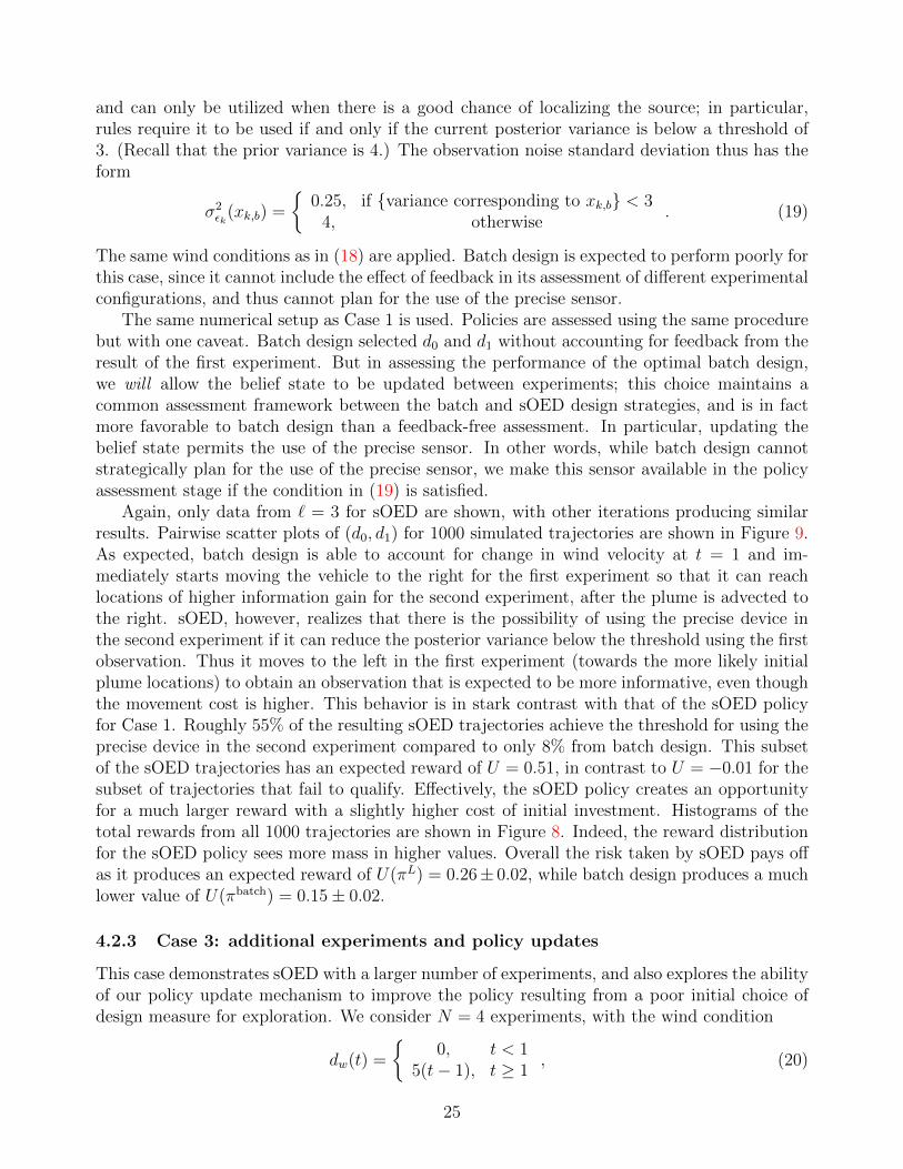
Overall, the tendency of the greedy design policy to “chase” high-information experimentalconfigurations turns out to be costly due to the quadratic movement penalty. This cost isreflected in Figure 8, which shows histograms of total reward from the trajectories. sOED

23

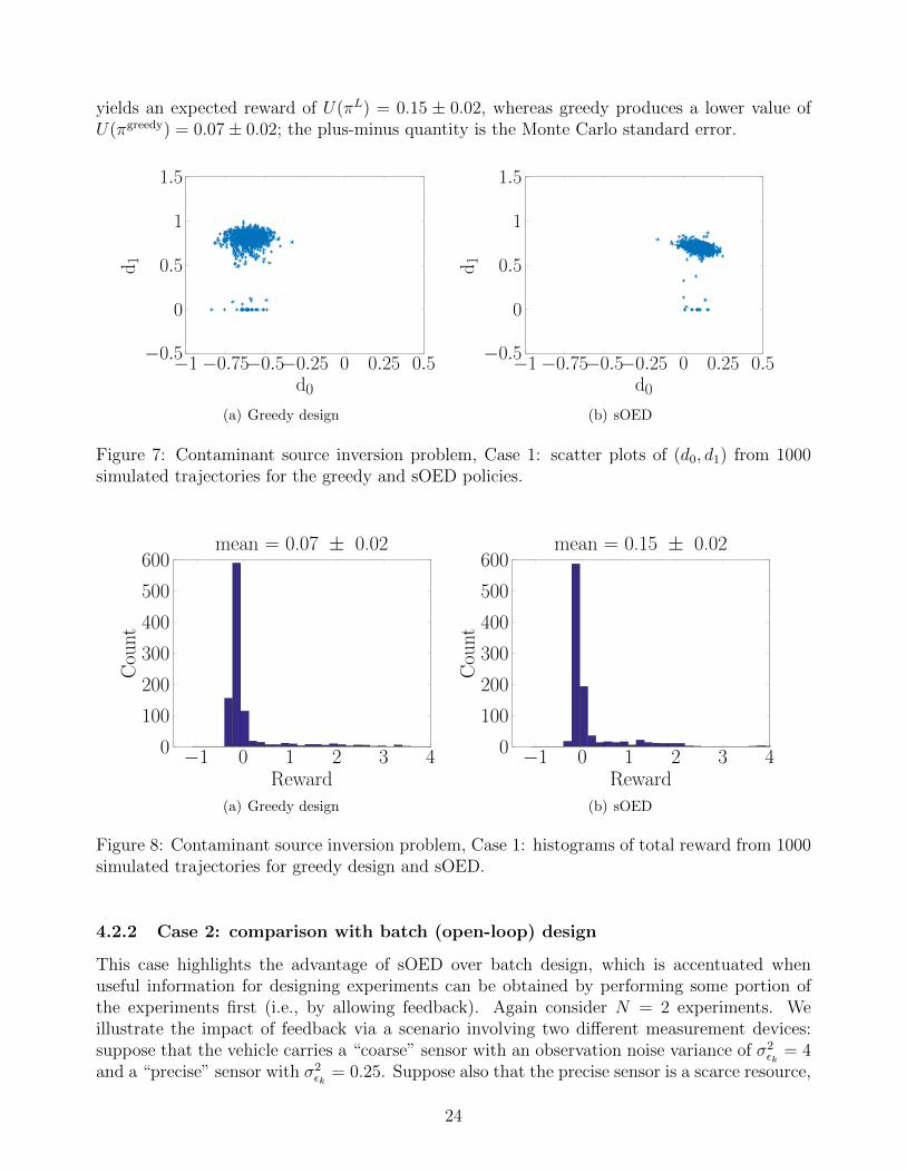
yields an expected reward of U(πL) = 0.15 ± 0.02, whereas greedy produces a lower value ofU(πgreedy) = 0.07± 0.02; the plus-minus quantity is the Monte Carlo standard error.

−1−0.75−0.5−0.25 0 0.25 0.5−0.5

0

0.5

1

1.5

d0

d1

(a) Greedy design

−1−0.75−0.5−0.25 0 0.25 0.5−0.5

0

0.5

1

1.5

d0

d1

(b) sOED

Figure 7: Contaminant source inversion problem, Case 1: scatter plots of (d0, d1) from 1000simulated trajectories for the greedy and sOED policies.

−1 0 1 2 3 40

100

200

300

400

500

600

Reward

Count

mean = 0.07 ± 0.02

(a) Greedy design

−1 0 1 2 3 40

100

200

300

400

500

600

Reward

Count

mean = 0.15 ± 0.02

(b) sOED

Figure 8: Contaminant source inversion problem, Case 1: histograms of total reward from 1000simulated trajectories for greedy design and sOED.

4.2.2 Case 2: comparison with batch (open-loop) design

This case highlights the advantage of sOED over batch design, which is accentuated whenuseful information for designing experiments can be obtained by performing some portion ofthe experiments first (i.e., by allowing feedback). Again consider N = 2 experiments. Weillustrate the impact of feedback via a scenario involving two different measurement devices:suppose that the vehicle carries a “coarse” sensor with an observation noise variance of σ2

εk= 4

and a “precise” sensor with σ2εk

= 0.25. Suppose also that the precise sensor is a scarce resource,

24

and can only be utilized when there is a good chance of localizing the source; in particular,rules require it to be used if and only if the current posterior variance is below a threshold of3. (Recall that the prior variance is 4.) The observation noise standard deviation thus has theform

σ2εk

(xk,b) =

{0.25, if {variance corresponding to xk,b} < 3

4, otherwise. (19)

The same wind conditions as in (18) are applied. Batch design is expected to perform poorly forthis case, since it cannot include the effect of feedback in its assessment of different experimentalconfigurations, and thus cannot plan for the use of the precise sensor.

The same numerical setup as Case 1 is used. Policies are assessed using the same procedurebut with one caveat. Batch design selected d0 and d1 without accounting for feedback from theresult of the first experiment. But in assessing the performance of the optimal batch design,we will allow the belief state to be updated between experiments; this choice maintains acommon assessment framework between the batch and sOED design strategies, and is in factmore favorable to batch design than a feedback-free assessment. In particular, updating thebelief state permits the use of the precise sensor. In other words, while batch design cannotstrategically plan for the use of the precise sensor, we make this sensor available in the policyassessment stage if the condition in (19) is satisfied.

Again, only data from ` = 3 for sOED are shown, with other iterations producing similarresults. Pairwise scatter plots of (d0, d1) for 1000 simulated trajectories are shown in Figure 9.As expected, batch design is able to account for change in wind velocity at t = 1 and im-mediately starts moving the vehicle to the right for the first experiment so that it can reachlocations of higher information gain for the second experiment, after the plume is advected tothe right. sOED, however, realizes that there is the possibility of using the precise device inthe second experiment if it can reduce the posterior variance below the threshold using the firstobservation. Thus it moves to the left in the first experiment (towards the more likely initialplume locations) to obtain an observation that is expected to be more informative, even thoughthe movement cost is higher. This behavior is in stark contrast with that of the sOED policyfor Case 1. Roughly 55% of the resulting sOED trajectories achieve the threshold for using theprecise device in the second experiment compared to only 8% from batch design. This subsetof the sOED trajectories has an expected reward of U = 0.51, in contrast to U = −0.01 for thesubset of trajectories that fail to qualify. Effectively, the sOED policy creates an opportunityfor a much larger reward with a slightly higher cost of initial investment. Histograms of thetotal rewards from all 1000 trajectories are shown in Figure 8. Indeed, the reward distributionfor the sOED policy sees more mass in higher values. Overall the risk taken by sOED pays offas it produces an expected reward of U(πL) = 0.26± 0.02, while batch design produces a muchlower value of U(πbatch) = 0.15± 0.02.

4.2.3 Case 3: additional experiments and policy updates

This case demonstrates sOED with a larger number of experiments, and also explores the abilityof our policy update mechanism to improve the policy resulting from a poor initial choice ofdesign measure for exploration. We consider N = 4 experiments, with the wind condition

dw(t) =

{0, t < 1

5(t− 1), t ≥ 1, (20)

25

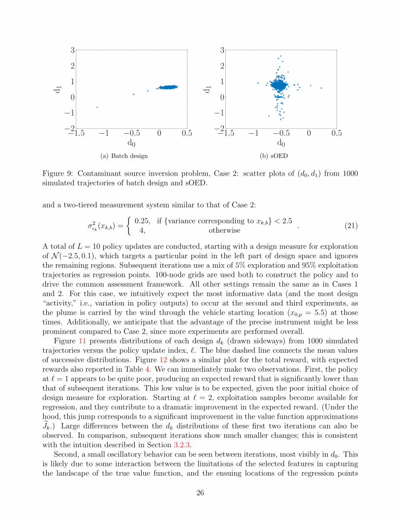
−1.5 −1 −0.5 0 0.5−2

−1

0

1

2

3

d0

d1

(a) Batch design

−1.5 −1 −0.5 0 0.5−2

−1

0

1

2

3

d0

d1

(b) sOED

Figure 9: Contaminant source inversion problem, Case 2: scatter plots of (d0, d1) from 1000simulated trajectories of batch design and sOED.

and a two-tiered measurement system similar to that of Case 2:

σ2εk

(xk,b) =

{0.25, if {variance corresponding to xk,b} < 2.5

4, otherwise. (21)

A total of L = 10 policy updates are conducted, starting with a design measure for explorationof N (−2.5, 0.1), which targets a particular point in the left part of design space and ignoresthe remaining regions. Subsequent iterations use a mix of 5% exploration and 95% exploitationtrajectories as regression points. 100-node grids are used both to construct the policy and todrive the common assessment framework. All other settings remain the same as in Cases 1and 2. For this case, we intuitively expect the most informative data (and the most design“activity,” i.e., variation in policy outputs) to occur at the second and third experiments, asthe plume is carried by the wind through the vehicle starting location (x0,p = 5.5) at thosetimes. Additionally, we anticipate that the advantage of the precise instrument might be lessprominent compared to Case 2, since more experiments are performed overall.

Figure 11 presents distributions of each design dk (drawn sideways) from 1000 simulatedtrajectories versus the policy update index, `. The blue dashed line connects the mean valuesof successive distributions. Figure 12 shows a similar plot for the total reward, with expectedrewards also reported in Table 4. We can immediately make two observations. First, the policyat ` = 1 appears to be quite poor, producing an expected reward that is significantly lower thanthat of subsequent iterations. This low value is to be expected, given the poor initial choice ofdesign measure for exploration. Starting at ` = 2, exploitation samples become available forregression, and they contribute to a dramatic improvement in the expected reward. (Under thehood, this jump corresponds to a significant improvement in the value function approximationsJk.) Large differences between the dk distributions of these first two iterations can also beobserved. In comparison, subsequent iterations show much smaller changes; this is consistentwith the intuition described in Section 3.2.3.

Second, a small oscillatory behavior can be seen between iterations, most visibly in d0. Thisis likely due to some interaction between the limitations of the selected features in capturingthe landscape of the true value function, and the ensuing locations of the regression points

26

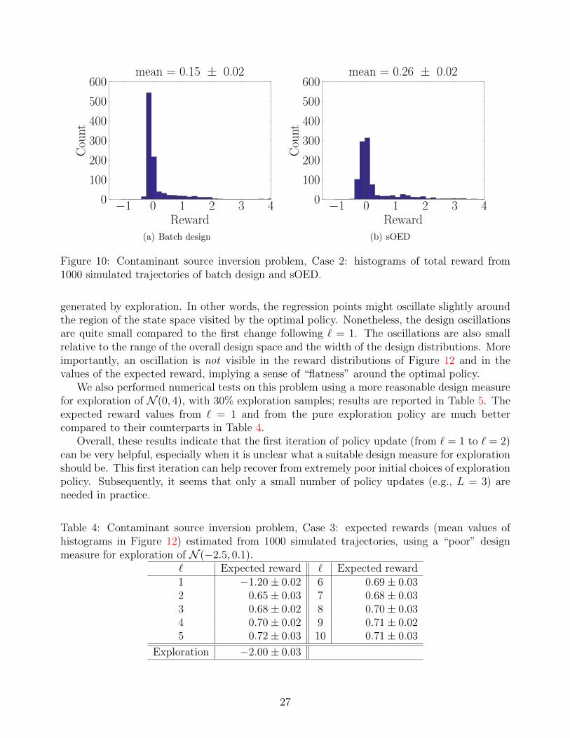
−1 0 1 2 3 40

100

200

300

400

500

600

Reward

Count

mean = 0.15 ± 0.02

(a) Batch design

−1 0 1 2 3 40

100

200

300

400

500

600

Reward

Count

mean = 0.26 ± 0.02

(b) sOED

Figure 10: Contaminant source inversion problem, Case 2: histograms of total reward from1000 simulated trajectories of batch design and sOED.

generated by exploration. In other words, the regression points might oscillate slightly aroundthe region of the state space visited by the optimal policy. Nonetheless, the design oscillationsare quite small compared to the first change following ` = 1. The oscillations are also smallrelative to the range of the overall design space and the width of the design distributions. Moreimportantly, an oscillation is not visible in the reward distributions of Figure 12 and in thevalues of the expected reward, implying a sense of “flatness” around the optimal policy.

We also performed numerical tests on this problem using a more reasonable design measurefor exploration of N (0, 4), with 30% exploration samples; results are reported in Table 5. Theexpected reward values from ` = 1 and from the pure exploration policy are much bettercompared to their counterparts in Table 4.

Overall, these results indicate that the first iteration of policy update (from ` = 1 to ` = 2)can be very helpful, especially when it is unclear what a suitable design measure for explorationshould be. This first iteration can help recover from extremely poor initial choices of explorationpolicy. Subsequently, it seems that only a small number of policy updates (e.g., L = 3) areneeded in practice.

Table 4: Contaminant source inversion problem, Case 3: expected rewards (mean values ofhistograms in Figure 12) estimated from 1000 simulated trajectories, using a “poor” designmeasure for exploration of N (−2.5, 0.1).

` Expected reward ` Expected reward1 −1.20± 0.02 6 0.69± 0.032 0.65± 0.03 7 0.68± 0.033 0.68± 0.02 8 0.70± 0.034 0.70± 0.02 9 0.71± 0.025 0.72± 0.03 10 0.71± 0.03

Exploration −2.00± 0.03

27

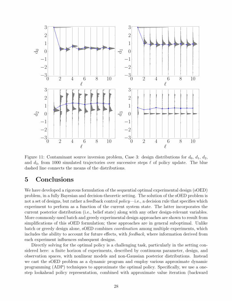
0 2 4 6 8 10−3

−2

−1

0

1

2

3

`

d0

0 2 4 6 8 10−3

−2

−1

0

1

2

3

`

d1

0 2 4 6 8 10−3

−2

−1

0

1

2

3

`

d2

0 2 4 6 8 10−3

−2

−1

0

1

2

3

`

d3

Figure 11: Contaminant source inversion problem, Case 3: design distributions for d0, d1, d2,and d3, from 1000 simulated trajectories over successive steps ` of policy update. The bluedashed line connects the means of the distributions.

5 Conclusions

We have developed a rigorous formulation of the sequential optimal experimental design (sOED)problem, in a fully Bayesian and decision-theoretic setting. The solution of the sOED problem isnot a set of designs, but rather a feedback control policy—i.e., a decision rule that specifies whichexperiment to perform as a function of the current system state. The latter incorporates thecurrent posterior distribution (i.e., belief state) along with any other design-relevant variables.More commonly-used batch and greedy experimental design approaches are shown to result fromsimplifications of this sOED formulation; these approaches are in general suboptimal. Unlikebatch or greedy design alone, sOED combines coordination among multiple experiments, whichincludes the ability to account for future effects, with feedback, where information derived fromeach experiment influences subsequent designs.

Directly solving for the optimal policy is a challenging task, particularly in the setting con-sidered here: a finite horizon of experiments, described by continuous parameter, design, andobservation spaces, with nonlinear models and non-Gaussian posterior distributions. Insteadwe cast the sOED problem as a dynamic program and employ various approximate dynamicprogramming (ADP) techniques to approximate the optimal policy. Specifically, we use a one-step lookahead policy representation, combined with approximate value iteration (backward

28

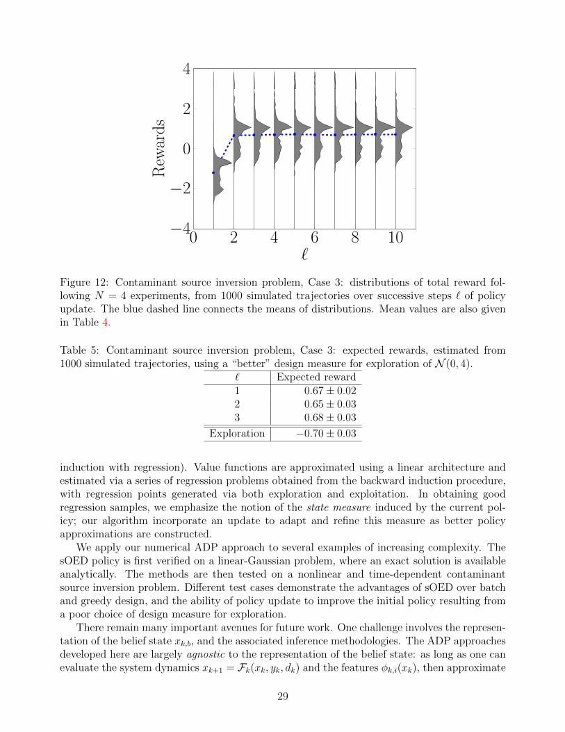
0 2 4 6 8 10−4

−2

0

2

4

`

Rew

ards

Figure 12: Contaminant source inversion problem, Case 3: distributions of total reward fol-lowing N = 4 experiments, from 1000 simulated trajectories over successive steps ` of policyupdate. The blue dashed line connects the means of distributions. Mean values are also givenin Table 4.

Table 5: Contaminant source inversion problem, Case 3: expected rewards, estimated from1000 simulated trajectories, using a “better” design measure for exploration of N (0, 4).

` Expected reward1 0.67± 0.022 0.65± 0.033 0.68± 0.03

Exploration −0.70± 0.03

induction with regression). Value functions are approximated using a linear architecture andestimated via a series of regression problems obtained from the backward induction procedure,with regression points generated via both exploration and exploitation. In obtaining goodregression samples, we emphasize the notion of the state measure induced by the current pol-icy; our algorithm incorporate an update to adapt and refine this measure as better policyapproximations are constructed.

We apply our numerical ADP approach to several examples of increasing complexity. ThesOED policy is first verified on a linear-Gaussian problem, where an exact solution is availableanalytically. The methods are then tested on a nonlinear and time-dependent contaminantsource inversion problem. Different test cases demonstrate the advantages of sOED over batchand greedy design, and the ability of policy update to improve the initial policy resulting froma poor choice of design measure for exploration.

There remain many important avenues for future work. One challenge involves the represen-tation of the belief state xk,b, and the associated inference methodologies. The ADP approachesdeveloped here are largely agnostic to the representation of the belief state: as long as one canevaluate the system dynamics xk+1 = Fk(xk, yk, dk) and the features φk,i(xk), then approximate

29

value iteration and all the other elements of our ADP algorithm can be directly applied. In thecase of parametric posteriors (e.g., Bayesian inference with conjugate priors and likelihoods)the representation and updating of xk,b is trivial. But in the general case of continuous andnon-Gaussian posteriors, finding an efficient representation of xk,b—one that allows repeatedinference under different realizations of the data—can be difficult. In this paper, we have em-ployed an adaptive discretization of the posterior probability density function, but this choiceis impractical for higher parameter dimensions. A companion paper will explore a more flexibleand scalable alternative, based on the construction of transport maps over the joint distri-bution of parameters and data, from which conditionals can efficiently be extracted [49, 45].Alternative ADP approaches are also of great interest, including model-free methods such asQ-learning.

Acknowledgments

The authors would like to acknowledge support from the Computational Mathematics Programof the Air Force Office of Scientific Research.

References

[1] A. Alexanderian, N. Petra, G. Stadler, and O. Ghattas, A Fast and ScalableMethod for A-Optimal Design of Experiments for Infinite-Dimensional Bayesian NonlinearInverse Problems, (2014), arXiv:1410.5899.

[2] A. C. Atkinson and A. N. Donev, Optimum Experimental Designs, Oxford UniversityPress, New York, NY, 1992.

[3] R. Bellman, Bottleneck Problems and Dynamic Programming, Proc. Natl. Acad. Sci. U.S. A., 39 (1953), pp. 947–951, http://dx.doi.org/10.1073/pnas.39.9.947.

[4] R. Bellman, Dynamic Programming and Lagrange Multipliers, Proc. Natl. Acad. Sci. U.S. A., 42 (1956), pp. 767–769, http://dx.doi.org/10.1073/pnas.42.10.767.

[5] I. Ben-Gal and M. Caramanis, Sequential DOE via dynamic programming, IIETrans. (Institute Ind. Eng., 34 (2002), pp. 1087–1100, http://dx.doi.org/10.1023/A:1019670414725.

[6] J. O. Berger, Statistical Decision Theory and Bayesian Analysis, Springer New York,New York, NY, 1985, http://dx.doi.org/10.1007/978-1-4757-4286-2.

[7] D. A. Berry, P. Muller, A. P. Grieve, M. Smith, T. Parke, R. Blazek,N. Mitchard, and M. Krams, Adaptive Bayesian Designs for Dose-Ranging Drug Tri-als, in Case Stud. Bayesian Stat., Springer New York, New York, NY, 2002, pp. 99–181,http://dx.doi.org/10.1007/978-1-4613-0035-9_2.

[8] D. P. Bertsekas, Dynamic Programming and Optimal Control, Vol. 1, Athena Scientific,Belmont, MA, 2005.

30

[9] D. P. Bertsekas, Dynamic Programming and Optimal Control, Vol. 2, Athena Scientific,Belmont, MA, 2007.

[10] D. P. Bertsekas and S. E. Shreve, Stochastic Optimal Control, Athena Scientific,Belmont, MA, 1996.

[11] D. P. Bertsekas and J. N. Tsitsiklis, Neuro-Dynamic Programming, Athena Scien-tific, Belmont, MA, 1996.

[12] F. Bisetti, D. Kim, O. Knio, Q. Long, and R. Tempone, Optimal Bayesianexperimental design for priors of compact support with application to shock-tube exper-iments for combustion kinetics, Int. J. Numer. Methods Eng., (2016), pp. 1–19, http:

//dx.doi.org/10.1002/nme.5211.

[13] G. E. P. Box and N. R. Draper, Empirical Model-Building and Response Surfaces,John Wiley & Sons, Hoboken, NJ, 1987.

[14] G. E. P. Box, J. S. Hunter, and W. G. Hunter, Statistics for Experimenters:Design, Innovation and Discovery, John Wiley & Sons, Hoboken, NJ, 2nd ed., 2005.

[15] A. E. Brockwell and J. B. Kadane, A Gridding Method for Bayesian SequentialDecision Problems, J. Comput. Graph. Stat., 12 (2003), pp. 566–584, http://dx.doi.

org/10.1198/1061860032274.

[16] P. Carlin, Bradley, J. B. Kadane, and A. E. Gelfand, Approaches for OptimalSequential Decision Analysis in Clinical Trials, Biometrics, 54 (1998), pp. 964–975, http://dx.doi.org/10.2307/2533849.

[17] D. R. Cavagnaro, J. I. Myung, M. A. Pitt, and J. V. Kujala, Adaptive DesignOptimization: A Mutual Information-Based Approach to Model Discrimination in Cog-nitive Science, Neural Comput., 22 (2010), pp. 887–905, http://dx.doi.org/10.1162/neco.2009.02-09-959.

[18] K. Chaloner and I. Verdinelli, Bayesian Experimental Design: A Review, Stat. Sci.,10 (1995), pp. 273–304, http://dx.doi.org/10.1214/ss/1177009939.

[19] J. A. Christen and M. Nakamura, Sequential Stopping Rules for Species Accumula-tion, J. Agric. Biol. Environ. Stat., 8 (2003), pp. 184–195, http://dx.doi.org/10.1198/108571103322161540.

[20] T. A. Cover and J. A. Thomas, Elements of Information Theory, John Wiley & Sons,Hoboken, NJ, 2nd ed., 2006.

[21] D. R. Cox and N. Reid, The Theory of the Design of Experiments, Chapman &Hall/CRC, Boca Raton, FL, 2000.

[22] H. A. Dror and D. M. Steinberg, Sequential Experimental Designs for GeneralizedLinear Models, J. Am. Stat. Assoc., 103 (2008), pp. 288–298, http://dx.doi.org/10.

1198/016214507000001346.

31

[23] C. C. Drovandi, J. M. McGree, and A. N. Pettitt, Sequential Monte Carlo forBayesian sequentially designed experiments for discrete data, Comput. Stat. Data Anal.,57 (2013), pp. 320–335, http://dx.doi.org/10.1016/j.csda.2012.05.014.

[24] C. C. Drovandi, J. M. McGree, and A. N. Pettitt, A Sequential Monte CarloAlgorithm to Incorporate Model Uncertainty in Bayesian Sequential Design, J. Comput.Graph. Stat., 23 (2014), pp. 3–24, http://dx.doi.org/10.1080/10618600.2012.730083.

[25] T. A. El Moselhy and Y. M. Marzouk, Bayesian inference with optimal maps, J.Comput. Phys., 231 (2012), pp. 7815–7850, http://dx.doi.org/10.1016/j.jcp.2012.07.022.

[26] V. V. Fedorov, Theory of Optimal Experiments, Academic Press, New York, NY, 1972.

[27] R. A. Fisher, The Design of Experiments, Oliver & Boyd, Edinburgh, United Kingdom,8th ed., 1966.

[28] S. Fujishige, Submodular Functions and Optimization, Elsevier, Amsterdam, The Nether-lands, 2nd ed., 2005, http://dx.doi.org/10.1016/S0167-5060(05)80003-2.

[29] J. Ginebra, On the Measure of the Information in a Statistical Experiment, BayesianAnal., 2 (2007), pp. 167–212, http://dx.doi.org/10.1214/07-BA207.

[30] G. J. Gordon, Stable Function Approximation in Dynamic Programming, in Proc. 12thInt. Conf. Mach. Learn., Tahoe City, CA, 1995, pp. 261–268, http://dx.doi.org/10.

1016/b978-1-55860-377-6.50040-2.

[31] I. Guyon, M. Nikravesh, S. Gunn, and L. A. Zadeh, Feature Extraction: Foun-dations and Applications, Springer Berlin Heidelberg, Berlin, Germany, 2006, http:

//dx.doi.org/10.1007/978-3-540-35488-8.

[32] E. Haber, L. Horesh, and L. Tenorio, Numerical methods for the design of large-scale nonlinear discrete ill-posed inverse problems, Inverse Probl., 26 (2010), p. 025002,http://dx.doi.org/10.1088/0266-5611/26/2/025002.

[33] X. Huan, Numerical Approaches for Sequential Bayesian Optimal Experimental Design,PhD thesis, Massachusetts Institute of Technology, 2015.

[34] X. Huan and Y. M. Marzouk, Simulation-based optimal Bayesian experimental designfor nonlinear systems, J. Comput. Phys., 232 (2013), pp. 288–317, http://dx.doi.org/10.1016/j.jcp.2012.08.013.

[35] X. Huan and Y. M. Marzouk, Gradient-Based Stochastic Optimization Methods inBayesian Experimental Design, Int. J. Uncertain. Quantif., 4 (2014), pp. 479–510, http://dx.doi.org/10.1615/Int.J.UncertaintyQuantification.2014006730.

[36] L. P. Kaelbling, M. L. Littman, and A. W. Moore, Reinforcement Learning: ASurvey, J. Artif. Intell. Res., 4 (1996), pp. 237–285, http://dx.doi.org/10.1613/jair.301.

32

[37] W. Kim, M. A. Pitt, Z.-L. Lu, M. Steyvers, and J. I. Myung, A HierarchicalAdaptive Approach to Optimal Experimental Design, Neural Comput., 26 (2014), pp. 2565–2492, http://dx.doi.org/10.1162/NECO_a_00654.

[38] A. Krause, A. Singh, and C. Guestrin, Near-Optimal Sensor Placements in GaussianProcesses: Theory, Efficient Algorithms and Empirical Studies, J. Mach. Learn. Res., 9(2008), pp. 235–284, http://dx.doi.org/10.1145/1102351.1102385.

[39] M. Lagoudakis, Least-Squares Policy Iteration, J. Mach. Learn. Res., 4 (2003), pp. 1107–1149.

[40] D. V. Lindley, On a Measure of the Information Provided by an Experiment, Ann. Math.Stat., 27 (1956), pp. 986–1005, http://dx.doi.org/10.1214/aoms/1177728069.

[41] H. Liu and H. Motoda, Feature Selection for Knowledge Discovery and Data Mining,Springer US, New York, NY, 1998, http://dx.doi.org/10.1007/978-1-4615-5689-3.

[42] Q. Long, M. Scavino, R. Tempone, and S. Wang, Fast estimation of expectedinformation gains for Bayesian experimental designs based on Laplace approximations,Comput. Methods Appl. Mech. Eng., 259 (2013), pp. 24–39, http://dx.doi.org/10.

1016/j.cma.2013.02.017.

[43] T. J. Loredo, Rotating Stars and Revolving Planets: Bayesian Exploration of the Pul-sating Sky, in Bayesian Stat. 9 Proc. Nineth Val. Int. Meet., Benidorm, Spain, 2010,pp. 361–392, http://dx.doi.org/10.1093/acprof:oso/9780199694587.003.0012.

[44] D. J. C. MacKay, Information Theory, Inference, and Learning Algorithms, CambridgeUniversity Press, Cambridge, United Kingdom, 4th ed., 2005, http://dx.doi.org/10.1198/jasa.2005.s54.

[45] Y. M. Marzouk, T. A. El Moselhy, M. D. Parno, and A. Spantini, An in-troduction to sampling via measure transport, in Handb. Uncertain. Quantif., SpringerInternational Publishing, 2016.

[46] P. Muller, D. A. Berry, A. P. Grieve, M. Smith, and M. Krams, Simulation-based sequential Bayesian design, J. Stat. Plan. Inference, 137 (2007), pp. 3140–3150,http://dx.doi.org/10.1016/j.jspi.2006.05.021.

[47] S. A. Murphy, Optimal dynamic treatment regimes, J. R. Stat. Soc. Ser. B (StatisticalMethodol., 65 (2003), pp. 331–355, http://dx.doi.org/10.1111/1467-9868.00389.

[48] D. Ormoneit and S. Sen, Kernel-Based Reinforcement Learning, Mach. Learn., 49(2002), pp. 161–178, http://dx.doi.org/10.1023/A:1017928328829.

[49] M. Parno and Y. Marzouk, Transport map accelerated Markov chain Monte Carlo,(2014), arXiv:1412.5492.

[50] W. B. Powell, Approximate Dynamic Programming: Solving the Curses of Dimension-ality, John Wiley & Sons, Hoboken, NJ, 2nd ed., 2011.

33

[51] M. L. Puterman, Markov Decision Processes: Discrete Stochastic Dynamic Program-ming, John Wiley & Sons, Hoboken, NJ, 1994.

[52] K. J. Ryan, Estimating Expected Information Gains for Experimental Designs With Ap-plication to the Random Fatigue-Limit Model, J. Comput. Graph. Stat., 12 (2003), pp. 585–603, http://dx.doi.org/10.1198/1061860032012.

[53] O. Sigaud and O. Buffet, Markov Decision Processes in Artificial Intelligence: MDPs,beyond MDPs and applications, John Wiley & Sons, Hoboken, NJ, 2010, http://dx.doi.org/10.1002/9781118557426.

[54] A. Solonen, H. Haario, and M. Laine, Simulation-Based Optimal Design Using aResponse Variance Criterion, J. Comput. Graph. Stat., 21 (2012), pp. 234–252, http:

//dx.doi.org/10.1198/jcgs.2011.10070.

[55] R. S. Sutton and A. G. Barto, Reinforcement Learning: An Introduction, The MITPress, Cambridge, MA, 1998.

[56] G. Terejanu, R. R. Upadhyay, and K. Miki, Bayesian experimental design for the ac-tive nitridation of graphite by atomic nitrogen, Exp. Therm. Fluid Sci., 36 (2012), pp. 178–193, http://dx.doi.org/10.1016/j.expthermflusci.2011.09.012.

[57] J. N. Tsitsiklis and B. Van Roy, An Analysis of Temporal-Difference Learning withFunction Approximation, IEEE Trans. Autom. Control (Institute Electr. Electron. Eng.,42 (1997), pp. 674–690, http://dx.doi.org/10.1109/9.580874.

[58] J. N. Tsitsiklis and B. Van Roy, Regression Methods for Pricing Complex American-Style Options, IEEE Trans. Neural Networks (Institute Electr. Electron. Eng., 12 (2001),pp. 694–703, http://dx.doi.org/10.1109/72.935083.

[59] C. Villani, Optimal Transport: Old and New, Springer-Verlag Berlin Heidelberg, Berlin,Germany, 2008.

[60] U. Von Toussaint, Bayesian inference in physics, Rev. Mod. Phys., 83 (2011), pp. 943–999, http://dx.doi.org/10.1103/RevModPhys.83.943.

[61] J. K. Wathen and J. A. Christen, Implementation of Backward Induction for Se-quentially Adaptive Clinical Trials, J. Comput. Graph. Stat., 15 (2006), pp. 398–413,http://dx.doi.org/10.1198/016214506X113406.

[62] C. J. C. H. Watkins, Learning from delayed rewards, PhD thesis, King’s College, 1989.

[63] C. J. C. H. Watkins and P. Dayan, Technical Note: Q-Learning, Mach. Learn., 8(1992), pp. 279–292, http://dx.doi.org/10.1023/a:1022676722315.

[64] B. P. Weaver, B. J. Williams, C. M. Anderson-Cook, and D. M. Higdon, Com-putational Enhancements to Bayesian Design of Experiments Using Gaussian Processes,Bayesian Anal., (2015), http://dx.doi.org/10.1214/15-BA945.

34