2006-151: A NEW APPROACH TO SOLVE BEAM DEFLECTION PROBLEMSUSING THE METHOD OF SEGMENTS

Hartley T. Grandin, Worcester Polytechnic InstituteHartley T. Grandin, Jr. is a Professor Emeritus of Engineering Mechanics and Design in theMechanical Engineering Department at Worcester Polytechnic Institute. He has authored thetextbook Fundamentals of the Finite Element Method that was published by Macmillan in 1986.Since his retirement from WPI in 1996, he teaches a mechanics of materials course each year andis currently writing the fifth draft of an introductory textbook with the co-author. In 1983 hereceived the WPI Board of Trustees’ Award for Outstanding Teaching. He received his B.S. in1955 and an M.S. in 1960 in Mechanical Engineering from Worcester Polytechnic Institute and aPh.D. in Engineering Mechanics from the Department of Metallurgy, Mechanics and MaterialsScience at Michigan State University in 1972. E-mail: hgrandin@rcn.com andhgrandin@wpi.edu.

Joseph Rencis, University of ArkansasJoseph J. Rencis is currently Professor and Head of the Department of Mechanical Engineering atthe University of Arkansas. From 1985 to 2004 he was in the Mechanical EngineeringDepartment at the Worcester Polytechnic Institute. His research focuses on the development ofboundary and finite element methods for analyzing solid, heat transfer and fluid mechanicsproblems. He serves on the editorial board of Engineering Analysis with Boundary Elements andis associate editor of the International Series on Advances in Boundary Elements. He is currentlywriting the fifth draft of an introductory mechanics of materials textbook with the author. He hasbeen the Chair of the ASEE Mechanics Division, received the 2002 ASEE New England SectionTeacher of the Year and is a fellow of the ASME. In 2004 he received the ASEE New EnglandSection Outstanding Leader Award and in 2006 the ASEE Mechanics Division James L. MeriamService Award. He received his B.S. from the Milwaukee School of Engineering in 1980, a M.S.from Northwestern University in 1982 and a Ph.D. from Case Western Reserve University in1985. V-mail: 479-575-3153; E-mail: jjrencis@uark.edu.

© American Society for Engineering Education, 2006

Page 11.79.1

A New Approach to Solve Beam Deflection Problems using the

Method of Segments

Abstract

This paper presents a new approach to solving beam deflection problems. The approach

involves the direct application of derived force-deformation formulas, a procedure commonly

used with axial and torsion bar problems. This direct application of derived force-deformation

formulas, referred to by the authors as Method of Segments, is extended to beam deflection

analysis in order to provide a solution procedure for beams that is consistent in philosophy and

application with that presented in most mechanics of materials textbooks for axially loaded bars

and torsionally loaded shafts. The beam force-deformation formulas, involving slope and

displacement, are derived by double integration for a beam of uniform cross-section, material

and distributed loading with end shear forces and couples. Application of the formulas is direct

and requires no integration or continuity equations. Furthermore, by identifying segments of

uniform geometry, material and distributed loading, this approach can easily be applied to beams

of discontinuous geometry and material that supports both concentrated and distributed loading.

Introduction

The great majority of undergraduate mechanics of materials textbooks1-50

directly apply

previously derived force-deformation formulas to problems involving the straight bar subjected

to centric axial loading and the straight circular cross-section bar (shaft) subjected to twisting

couples. In both cases, the bars are uniform in cross-section and material, and the concentrated

loads are applied at the ends and distributed loads are continuous along the full length. The

force-deformation formulas are shown in Figures 1 and 2 for bars subjected to centric axial

loading and twisting couples, respectively. These formulas, referred to as Material Law

Formulas by the authors, are commonly found in mechanics of materials textbooks1-50

.

L

FF

y

x

uu u(x)

aa

a

b

b

b

p, force/length

x

Figure 1. Material Law Formulas for a uniform bar with end centric axial and

centric uniform distributed loads plus temperature change.

Page 11.79.2

yL

x

ba

a

φa

T

bT

x

q, moment/length

φbφ(x)

Figure 2. Material Law Formulas for a uniform shaft with end torsional couples and

uniform distributed torsional couple.

In a real application, an axially loaded bar, for example, the bar may have any

combination of cross section size and shape, material and applied concentrated or distributed

loadings. Figure 3 illustrates a ‘complex’ bar which has two lengths of different, but

individually continuous, cross-sections, loading and, perhaps, material. This bar of

discontinuous cross-section, load and material can be treated as an assemblage of two simpler

bars, called segments, of uniform cross-section with continuous loading along each length of

uniform material as shown in Figures 3b and 3c. The effects of the loading on each segment can

be combined to obtain the resultant effect on the total, more complex composite bar. Solutions

are obtained by application of point compatibility and a summation of the relative displacements

of the simple bar segments. The method to solve this type of problem is referred to by the

authors as the Method of Segments. In mechanics of materials textbooks, the method is applied

to the axially loaded bar and torsionally loaded shaft, but not the beam. The procedure is

referred to as the discrete element method by Bauld1. Other textbooks do not explicitly call it a

method, but the segments are referred to as component parts or portions2,3

, elements9,20,27-29

,

parts14,15,16,22,33,47

, portion6, section

26, section or segment

7, segment

5,31,48 and segment and

region17,18

.

AC

d2d1

L L

B

PC

(2)(1)

p (force/length)

(1)

A BB C

FB

FB

(2)

FA

L L

p1 2

1 2

Uniform Load on Segment (2)

PB

PB

(a) Problem Definition

(b) Free-body Diagram I (c) Free-body Diagram II

PC

Figure 3. Two segment determinate bar problem with concentrated loads and distributed load.

Page 11.79.3

The authors are not aware of any work that has used the Method of Segments to solve

beam deflection problems and wish to show how this method may be used to solve beam

bending problems. The Material Law Formulas for a uniform beam supporting a uniformly

distributed load and end shear forces and bending couples will first be developed. The analysis

process proposed by the authors to solve problems51

will be discussed and will be used to solve

determinate and indeterminate beam problems. A review of current beam deflection methods

will be considered. Finally, the advantages and disadvantages of this proposed Method of

Segments will be presented.

Development of Beam Material Law Formulas

In this section the Material Law Formulas for a straight beam of uniform cross section

and material with end and uniformly distributed transverse loading is developed using the double

integration method. The double integration method is found in nearly all mechanics of materials

textbooks.

Free-Body Diagram I in Figure 4 is of a linearly elastic, homogeneous (constant elastic

modulus E), beam of length L, uniform cross section (constant zI ), with positive internal shear

forces AsF and

BsF and positive internal bending couples MA and MB acting at the ends. The

beam supports a uniformly distributed downward load, w, force/length. All points in the beam,

including the end points ‘A’ and ‘B’, undergo positive transverse displacement, v(x), in the

positive Y direction. At all points in the beam, including the end points ‘A’ and ‘B’, the beam

neutral surface undergoes rotation ( )xθ , with the positive sense as shown in Figure 4 at the end

points ‘A’ and ‘B.’ Free-Body Diagram II in Figure 4 is of the partial length of the beam

produced by cutting the beam at an arbitrary location x. For this beam, the following will be

derived:

• Functions defining the internal shear force, Fs(x) = ABsF , the internal bending couple M(x) =

MAB, the slope of the neutral surface (or axis), ABx θθ =)( and transverse displacement of the

neutral surface (or axis), v(x) = vAB, at any cross section location in the beam.

• Functions relating the internal shear forces

AsF and BsF and bending couples MA and MB at

the ends to the rotational and transverse displacements ABA v,, θθ and Bv at the ends.

The derivations are based on principles of equilibrium, Hooke’s Law and the differential

equation for beam elastic deflection 2

2z z

d vM EI

dx

=

.

Page 11.79.4

X, xBAMA M

BF F

vA

vB

θB

Y

L

xB

x

xA

FBD I

AMAF

MF

FBD II

s

w

s s

s

A B

AAB

AB

DisplacedNeutral Surface

θA

w, force/length

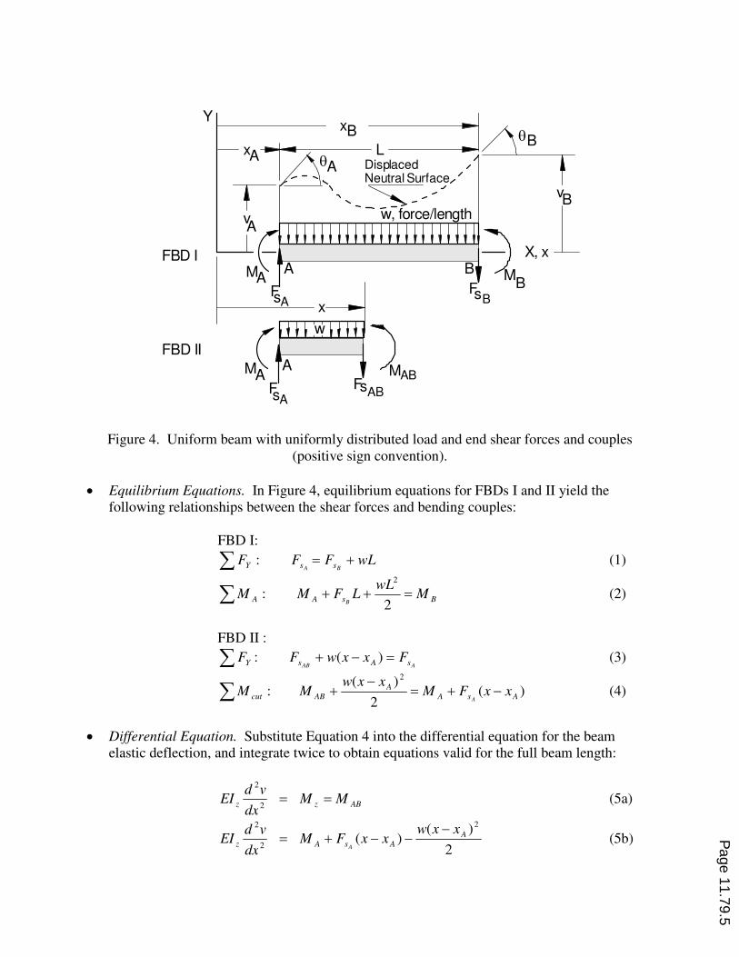
Figure 4. Uniform beam with uniformly distributed load and end shear forces and couples

(positive sign convention).

• Equilibrium Equations. In Figure 4, equilibrium equations for FBDs I and II yield the

following relationships between the shear forces and bending couples:

FBD I:

∑ += wLFFFBA ssY : (1)

BsAA MwL

LFMMB

=++∑2

:2

(2)

FBD II :

∑ =−+AAB sAsY FxxwFF )(: (3)

)(2

)(:

2

AsA

A

ABcut xxFMxxw

MMA

−+=−

+∑ (4)

• Differential Equation. Substitute Equation 4 into the differential equation for the beam

elastic deflection, and integrate twice to obtain equations valid for the full beam length:

ABzz MMdx

vdEI ==

2

2

(5a)

2

)()(

2

2

2

A

AsAz

xxwxxFM

dx

vdEI

A

−−−+= (5b) P

age 11.79.5

θθ

dEIdxdx

dEIdx

dx

vdEI zzz ==

2

2

[ ] dxxxw

dxxxFMdEI A

AsAz A 2

)()(

2−−−+=θ (6)

EIz

2( ) ( )

( )2

θ

θ

βθ β β

−= + − −

∫ ∫ A

A A

x xA

A s Ax

w xd M F x d

2)(

2)()( A

z

s

A

z

A

AAB xxEI

Fxx

EI

Mx A −+−+== θθθ

6

)( 3

Axxw −− (7)

dvdxdx

dvdxx ==)(θ

dxxxEI

Fdxxx

EI

Mdxdv A

z

s

A

z

A

A

A 2)(2

)( −+−+= θ

dxEI

xxw

z

A

6

)( 3−− (8)

( )

2( ) ( )2

θ β β β β= + − + −∫ ∫ ∫ ∫ A

A A A A

v x x x x sAA A A

v x x xz z

FMdv dx x d x d

EI EI

3( )

6A

xA

xz

w xd

EI

ββ

−−∫ (9)

32 )(6

)(2

)()( A

z

s

A

z

A

AAAAB xxEI

Fxx

EI

Mxxvvxv A −+−+−+== θ

z

A

EI

xxw

24

)( 4−− (10)

Substitution of x = xB and L = xB - xA into Equations 7 and 10 yields the following

formulas for the end B slope and transverse displacement in terms of the distributed load, the

shear force and couple at end A and the slope and transverse displacement at end A:

zz

s

z

A

ABEI

wL

EI

LF

EI

LMA

62

32

−++= θθ (11)

zz

s

z

A

AABEI

wL

EI

LF

EI

LMLvv A

2462

432

−+++= θ (12)

Page 11.79.6

It is preferable to have formulas with the dependent displacements at one end as a function of

forces at the same end. In application, this would mean that the independent position variable

would be the same for the displacements and forces. Substitution of Equations 1 and 2 into

Equations 11 and 12 yields formulas which define the end B slope and transverse displacement

in terms of the distributed load, the shear force and couple at end B and the slope and transverse

displacement at end A:

zz

s

z

BAB

EI

wL

EI

LF

EI

LMB

62

32

−−+= θθ (13)

zz

s

z

B

AABEI

wL

EI

LF

EI

LMLvv B

832

432

−−++= θ (14)

These two formulas will be referred to as the Material Law Formulas for the end loaded beam

and are presented in Figure 5 with general representative symbols ‘a’ and ‘b’. In applying the

Material Law Formulas, the symbols ‘a’ and ‘b’ are replaced by the letters assigned to the ends

of each segment in the problem being analyzed. It is important to appreciate that the Material

Law algebraic equations have been derived by the double integration method. Application of

these formulas to any beam problem is done without the need for additional integration or

solution for constants of integration.

The Material Law Formulas shown in Figure 5 is limited to a beam which has end loads,

a uniformly distributed loading, uniform geometry and material for the entire beam length. We

want to show how this special case can be used to solve beam problems which are complicated

to the extent of having discontinuous loading functions, cross-sectional areas and materials, all in

the same beam. The analysis process that will be used to solve beam problems will first be

discussed and then two example problems will illustrate the application of the Material Law

Formulas.

X, x

M MF

a ba b

s sba

Y w, force/length

L

F

Figure 5. Material Law Formulas for a uniform beam with end shear forces and bending couples

and uniformly distributed load.

Page 11.79.7

Analysis Process

The authors use an approach to mechanics of materials that integrates theory, analysis,

verification and design51

. The analysis component uses a non-traditional structured problem

solving format containing eight steps. The students are required to follow the appropriate steps

listed below to solve any problem.

1. Model. The success of any analysis is highly dependent on the validity and

appropriateness of the model used to predict and analyze its behavior in a real system,

whether centric axial loading, torsion, bending or a combination of the above.

Assumptions and limitations need also be stated. This step is not explicitly emphasized

in any mechanics of materials textbook.

2. Free-Body Diagrams. This step is where all the free-body diagrams initially thought to

be required for the solution are drawn. The free-body diagrams include the complete

structure and/or parts of the structure. Very importantly, all dimensions and loads, even

those which are known, are defined symbolically.

3. Equilibrium Equations. The equilibrium equations for each free-body diagram required

for a solution are written. All equations are formulated symbolically. There is no

attempt made at this point to isolate the unknown variables. However, every term in each

equation must be examined for dimensional homogeneity.

4. Material Law Formulas. The material law formulas are written for each part of a

structure based on the Model in Step 1. All equations are formulated symbolically and

there is no algebraic manipulation. Every term in each equation must be examined for

dimensional homogeneity.

5. Compatibility and Boundary Conditions. One or more compatibility equations are written

in symbolic form to relate the displacements. A compatibility diagram is used when

appropriate to assist in developing the compatibility equations. All equations are

formulated symbolically and there is no algebraic manipulation. Every term in each

equation must be examined for dimensional homogeneity. Although compatibility

equations are commonly written for indeterminate problems, the authors emphasize their

use for determinate problems just as is done in the textbooks by Craig9, Crandall

10 et al.,

Shames37

, and Shames & Pitarresi38

.

6. Complementary and Supporting Formulas. Steps 1 through 5 are sufficient to solve for

the (primary) variables for force and displacement in a structures problem. Step 6

includes complementary formulas for other (secondary) variables such as stress and

strain, variables which may govern the maximum allowable in service values of force and

displacement, but which do not affect the governing equilibrium or deformation

equations. Supporting formulas are those which might be required to supply variable

values in the Material Law equations and complementary formulas; formulas such as

area, moment of inertia, centroid location of a cross-section, volume, etc. The

complementary and supporting formulas are written symbolically and are necessary to

develop a complete analysis.

Page 11.79.8

7. Solve. The independent equations developed in Steps 3 through 6 solve the problem.

The students compare the number of independent equations and the number of

unknowns. The authors emphasize that the student should not proceed until the number

of unknowns equals the number of independent equations.

The solution may be obtained by hand, and this generally requires algebraic

manipulation. Alternatively, the solution of any number of equations, linear or non-

linear, can be obtained with a modern engineering tool. With intelligent application of

verification (Step 8), the computer program is a much more reliable calculation device

than a calculator. (ABET52

criterion 3(k) states that engineering programs must

demonstrate that their students have the “ability to use the techniques, skills, and modern

engineering tools necessary for engineering practice”.) The students are allowed to select

the modern engineering tool of their choice, and this might include Mathcad53

, Matlab54

and TKSolver55

. The authors have not seen this solution procedure in any mechanics of

materials textbook.

8. Verify. One of our educational goals is to convince students of the wisdom to question

and test solutions to verify their ‘answers’. The verify Step 8 is carried out after solution

Step 7 is performed once. The power of our proposed use of the modern engineering tool

rests in the ability to quickly and easily run many cases to verify the problem solution.

How does one test the problem solution? Some suggested questions that students may

apply for the purpose of verification of their ‘answers’ are as follows: a. A hand

calculation?; b. Comparison with a known problem solution?; c. Examination of limiting

cases with known solutions?; d. Examination of the obvious solution?; e. Your best

judgment?; f. Comparison with experimentation (not considered)?. As indicated,

attempts at solution verification may take many forms, and, although in some cases it

may not yield absolute proof, it does improve the level of confidence. This step is

considered only in the mechanics of materials textbook by Craig9.

Problems in statics require only Steps 1, 2, 3, 6 and 7. These five steps have not been employed

in the treatment of statics problems in any statics or mechanics of materials textbook.

Furthermore, Steps 1 through 8 have not been suggested in any mechanics of materials textbook.

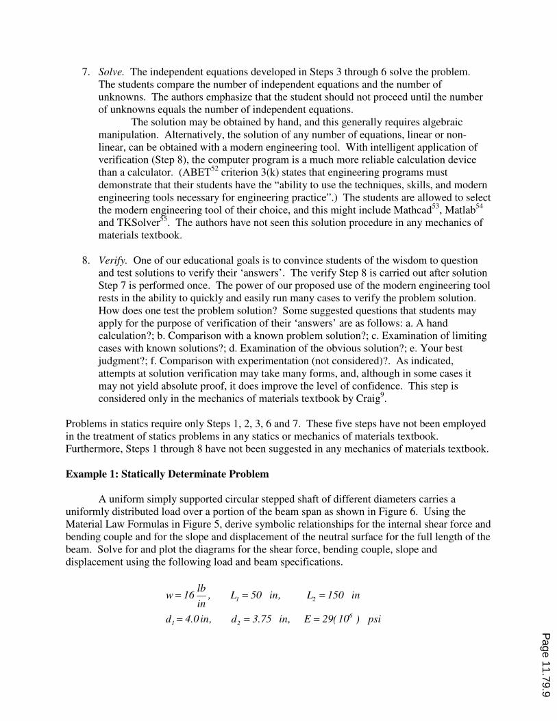
Example 1: Statically Determinate Problem

A uniform simply supported circular stepped shaft of different diameters carries a

uniformly distributed load over a portion of the beam span as shown in Figure 6. Using the

Material Law Formulas in Figure 5, derive symbolic relationships for the internal shear force and

bending couple and for the slope and displacement of the neutral surface for the full length of the

beam. Solve for and plot the diagrams for the shear force, bending couple, slope and

displacement using the following load and beam specifications.

= = =

= = =

1 2

6

1 2

lbw 16 , L 50 in, L 150 in

in

d 4.0 in, d 3.75 in, E 29(10 ) psi

Page 11.79.9

Y

C

L

L L 1 2

B

d2

X, xA

d1

w, force/length

Figure 6. Simply supported stepped shaft with partial distributed load.

SOLUTION:

The analysis process is based on the eight steps discussed in the previous section.

1. Model. The simply supported beam carries a distributed transverse load over a portion of

the span. In order to use the Material Law in Figure 5, the beam must be divided into

segments, each having uniform cross-section inertia and material properties and loading

consisting of end shear forces, end bending couples and a uniformly distributed load. This

segment division is shown in Figure 7. With the exception of FBD I, all diagrams satisfy

these segment requirements.

2. Free-Body Diagrams. The free-body diagrams are shown in Figure 7. The partial segment

FBDs II and III are drawn because we wish to derive the solution for shear force, bending

couple and neutral surface slope and displacement for the entire length of the beam. These

diagrams will provide expressions at the arbitrary x locations. Free-body diagrams IV and

V are necessary to define the solution at the specific boundary supports and segment

junctures.

Note that the applied beam load, w, is carried on segment (1), the distributed load on

segment (2) is zero. Also note, the internal shear force )1(

BsF and bending couple, )1(

BM ,

although labeled to be considered in the segment (1) side of the slice at location B, are single

valued at B, there is no applied force or couple at B to produce a discontinuity in either the

internal force or couple.

Page 11.79.10

RC

Segment (1) Segment (2)

Y

FBD I BRA

(1)

sAB

FBD IIM

x

x

(2)

F F

M FBD III

RA

Segment (1)

M

FBD IV

A B

RC

Segment (2)

F

B C

FBD V

L L 1 2

(1)

(1)

(1)

X, x

w, force/length

w

w, force/length

M

sBCsB(1)

R

AB

BC

B

(1)

sB(1)

A

B

sB

M

F

F

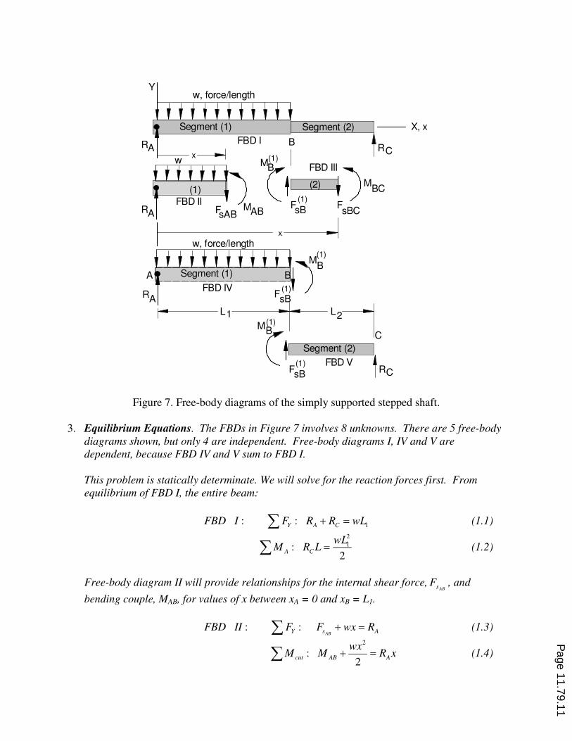
Figure 7. Free-body diagrams of the simply supported stepped shaft.

3. Equilibrium Equations. The FBDs in Figure 7 involves 8 unknowns. There are 5 free-body

diagrams shown, but only 4 are independent. Free-body diagrams I, IV and V are

dependent, because FBD IV and V sum to FBD I.

This problem is statically determinate. We will solve for the reaction forces first. From

equilibrium of FBD I, the entire beam:

1: :Y A CFBD I F R R wL+ =∑ (1.1)

2

1:2

A C

wLM R L =∑ (1.2)

Free-body diagram II will provide relationships for the internal shear force,ABsF , and

bending couple, MAB, for values of x between xA = 0 and xB = L1.

: :ABY s AFBD II F F wx R+ =∑ (1.3)

2

:2

cut AB A

wxM M R x+ =∑ (1.4)

Page 11.79.11

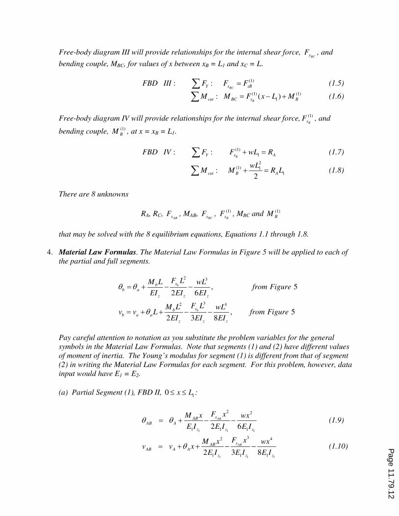
Free-body diagram III will provide relationships for the internal shear force, BCsF , and

bending couple, MBC, for values of x between xB = L1 and xC = L.

(1): :BCY s sBFBD III F F F=∑ (1.5)

(1) (1)

1: ( )Bcut BC s BM M F x L M= − +∑ (1.6)

Free-body diagram IV will provide relationships for the internal shear force,)1(

BsF , and

bending couple, )1(

BM , at x = xB = L1.

(1)

1: :BY s AFBD IV F F wL R+ =∑ (1.7)

2

(1) 11:

2cut B A

wLM M R L+ =∑ (1.8)

There are 8 unknowns

RA, RC, ABsF , MAB,

BCsF , )1(

BsF , MBC and )1(

BM

that may be solved with the 8 equilibrium equations, Equations 1.1 through 1.8.

4. Material Law Formulas. The Material Law Formulas in Figure 5 will be applied to each of

the partial and full segments.

2 3

32 4

, 52 6

, 52 3 8

b

b

sbb a

z z z

sbb a a

z z z

F LM L wLfrom Figure

EI EI EI

F LM L wLv v L from Figure

EI EI EI

θ θ

θ

= + − −

= + + − −

Pay careful attention to notation as you substitute the problem variables for the general

symbols in the Material Law Formulas. Note that segments (1) and (2) have different values

of moment of inertia. The Young’s modulus for segment (1) is different from that of segment

(2) in writing the Material Law Formulas for each segment. For this problem, however, data

input would have E1 = E2.

(a) Partial Segment (1), FBD II, 10 x L≤ ≤ :

1 1 1

2 2

1 1 12 6

ABsABAB A

z z z

F xM x wx

E I E I E Iθ θ= + − − (1.9)

1 1 1

32 4

1 1 12 3 8

ABsABAB A A

z z z

F xM x wxv v x

E I E I E Iθ= + + − − (1.10)

Page 11.79.12

(b) Partial Segment (2), FBD III, 1L x L≤ ≤ :

2 2

2

11

2 2

( )( )

2

BCsBCBC B

z z

F x LM x L

E I E Iθ θ

−−= + − (1.11)

2 2

3211

1

2 2

( )( )( )

2 3

BCsBCBC B B

z z

F x LM x Lv v x L

E I E Iθ

−−= + − + − (1.12)

(c) Full Segment (1), FBD IV:

1 1 1

(1) 2(1) 311 1

1 1 12 6

BsBB A

z z z

F LM L wL

E I E I E Iθ θ= + − − (1.13)

1 1 1

(1) 3(1) 2 411 1

1 1 12 3 8

BsBB A A B

z z z

F LM L wLv v x

E I E I E Iθ= + + − − (1.14)

(d) Full Segment (2), FBD V: Note that the right end couple and the distributed load are

zero, and the support reaction RC results in a negative internal shear force at end C:

Css

Cb

RFF

MM

Cb−=⇒

=⇒ 0

2

2

2

2

( )

2

CC B

z

R L

E Iθ θ

−= − (1.15)

2

3

22

2

( )

3

CC B B

z

R Lv v L

E Iθ

−= + − (1.16)

5. Compatibility and Boundary Conditions. The beam has been separated into two segments

for analysis, and the segments must be rejoined. The fact that the right end of segment (1)

and the left end of segment (2) are attached is assured by providing the same slope and

displacement symbol designation for each segment at the juncture.

The boundary conditions for this beam are established by the rigid pin and roller supports at

A and C.

0

0

=

=

C

A

v

v

6. Complementary and Supporting Formulas. In general, formulas would be applied here to

calculate stress and the area moment of inertia. In this example, we require the area moment

of inertia for segments (1) and (2).

1

4

1

64z

dI

π= (i)

Page 11.79.13

2

4

2

64z

dI

π= (ii)

7. Solve. Some things should be apparent in this solution formulation; integration is not

required, it has already been done, and there are no constants of integration to be

determined.

Considering the boundary values as known, there are an additional 8 unknowns generated in

writing the Material Law equations

θAB, θA, vAB, θBC, θB, vBC, vB and θC

Thus, in summary, we have a total of the following 16 unknowns

RA, RC, ABsF , MAB,

BCsF , )1(

BsF , MBC and )1(

BM

θAB, θA, vAB, θBC, θB, vBC, vB and θC

which can be solved with the 8 equilibrium equations, Equations 1.1 through 1.8, and the

additional 8 Material Law Formulas, Equations 1.9 through 1.16. The equations will be

solved with an equation solver, e.g., MathCad53

, MatLab54

or TKSolver55

.

The following results are presented for forces and displacements at locations A, B and C.

RA = 700 lb, RC = 100 lb

)1(

BsF = −100 lb, )1(

BM = 15000 lb · in

θA = −3.26 (10-3

) rad, θB = −1.77 (10-3

) rad, θC = 2.23 (10-3

) rad

vB = −1.34 (10−1

) in

The diagrams in Figure 8 are plots of the dependent variables over the full length of the

beam.

8. Verify. Test the solution.

• Setting the distributed load w = 0 will yield the obvious solution of a zero response.

• Changing the sign of the distributed load will result in reactions of the same magnitude

but opposite direction.

• Run a solution with a distributed load, constant material and constant moment of inertia

over the full span and check for symmetry and compare the value of maximum

displacement and end rotations with other sources found in a handbook (v(L/2) =

-5wL4/384EIz and θ(0) = - θ(L) = - wL

3/24EIz). The reaction forces will also be RA = RB

= wL/2.

• The best approach to the solution of a problem like this is to plot all of the dependent

variables as has been done in Figure 8. Gaps in the diagrams, discontinuities which

should not exist, failure to match boundary values, etc., can flash a warning that

something is not right.

• Calculate and check intermediate values by hand.

Page 11.79.14

Two other checks the authors have found to be helpful for all problems are:

• Double check the input.

• Go back and check the solution after a few days.

(a) Internal Shear Force vs Position

(b) Internal Couple vs Position

(c) Neutral Axis Slope vs Position

(d) Neutral Axis Displacement vs Position

Figure 8. Shear, bending couple, slope and displacement diagrams for simply

supported beam.

Example 2: Statically Indeterminate Problem

Consider the beam shown in Figure 9. It is solidly built into the wall at the left end, and

supported on the roller at the right end. A couple, CB, of known magnitude is applied to the right

end. Solve, using the Material Law Formulas in Figure 5, for the symbolic relationships for the

reaction forces exerted by the wall, end A, and the roller at end B.

(a) Internal Shear Force vs

Position

(b) Internal Couple vs

Position

(c) Neutral Axis Slope vs

Position

(d) Neutral Axis Displacement vs

Position

Page 11.79.15

B

B

xA

C

Y

L

Figure 9. Propped cantilever beam with concentrated couple.

SOLUTION:

1. Model. The full beam satisfies the requirements of the Material Law beam model; one length

with continuous material, geometry, distributed load (zero) and end loads. Therefore, the

full beam may be used, there is no need to establish smaller segments.

2. Free-Body Diagrams. The free-body diagram of the full beam is shown in Figure 10.

RB

BM A FBD I

C

RA

x

Y

Figure 10. Free-body diagram of the propped cantilever beam.

3. Equilibrium Equations. The force and moment equilibrium equations for the beam

reaction forces in Figure 10 are as follows:

RA+RB = 0 (2.1)

MA+RAL = CB (2.2)

Given the couple CB, there are three unknowns, RA, RB and MA. Since there are only two

independent equilibrium equations, these equations alone are insufficient to solve for the

unknowns; the problem is statically indeterminate. Therefore, the deformation properties of

the beam must be introduced.

4. Material Law Formulas. The Material Law Formulas will be applied to the full beam:

2 3

, 52 6

bsbb a

z z z

F LM L wLfrom Figure

EI EI EIθ θ= + − −

Page 11.79.16

32 4

, 52 3 8

bsbb a a

z z z

F LM L wLv v L from Figure

EI EI EIθ= + + − −

Relating the problem variables and values to the symbols in the formulas, we have:

0w,RFF,CMM

vv,,

BssBBb

BbAaBb

Bb=−=⇒=⇒

⇒⇒⇒ θθθθ

Substituting into the Material Law Formulas yields

z

2

B

z

BAB

EI2

L)R(

EI

LC −−+= θθ (2.3)

z

B

z

BAAB

EI

L)R(

EI

LCLvv

32

32 −−++= θ (2.4)

5. Boundary Conditions. The boundary conditions for this beam are:

vA = 0

θA = 0

vB = 0

6. Complementary and Supporting Formulas. In general, formulas would be applied here to

calculate the area moment of inertia.

7. Solve. There are four unknowns as follows:

RA, RB, MA and θA

which can be solved using Equations 2.1 through 2.4. As an alternative to using an equation

solver, the problem will be solved by hand to obtain symbolic formulas for the solution.

Substituting the boundary conditions into Equations 2.3 and 2.4 yields the following:

(i)

2

2 3

( )0

2

( )0 0 0

2 3

B BB

z z

B B

z z

C L R L

EI EI

C L R L

EI EI

θ−

= + −

−= + + −

(ii)

Solving Equation ii for the reaction force RB yields:

L

CR B

B2

3−=

Page 11.79.17

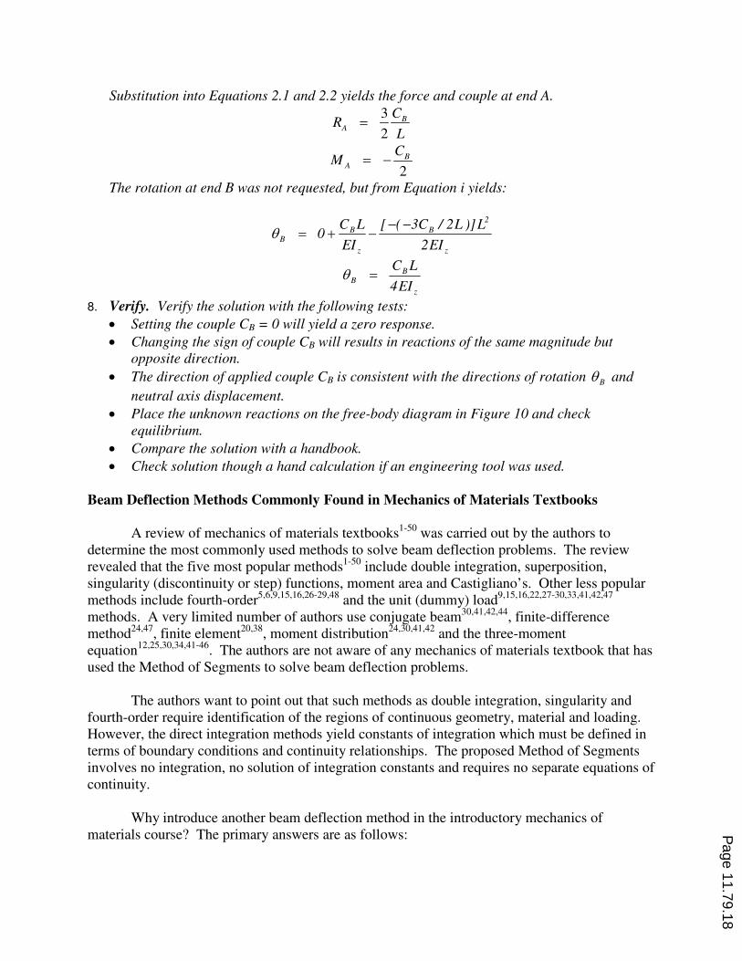
Substitution into Equations 2.1 and 2.2 yields the force and couple at end A.

3

2

BA

CR

L=

2

BA

CM = −

The rotation at end B was not requested, but from Equation i yields:

z

2

B

z

BB

EI2

L)]L2/C3([

EI

LC0

−−−+=θ

z

BB

EI4

LC=θ

8. Verify. Verify the solution with the following tests:

• Setting the couple CB = 0 will yield a zero response.

• Changing the sign of couple CB will results in reactions of the same magnitude but

opposite direction.

• The direction of applied couple CB is consistent with the directions of rotation Bθ and

neutral axis displacement.

• Place the unknown reactions on the free-body diagram in Figure 10 and check

equilibrium.

• Compare the solution with a handbook.

• Check solution though a hand calculation if an engineering tool was used.

Beam Deflection Methods Commonly Found in Mechanics of Materials Textbooks

A review of mechanics of materials textbooks1-50

was carried out by the authors to

determine the most commonly used methods to solve beam deflection problems. The review

revealed that the five most popular methods1-50

include double integration, superposition,

singularity (discontinuity or step) functions, moment area and Castigliano’s. Other less popular

methods include fourth-order5,6,9,15,16,26-29,48

and the unit (dummy) load9,15,16,22,27-30,33,41,42,47

methods. A very limited number of authors use conjugate beam30,41,42,44

, finite-difference

method24,47

, finite element20,38

, moment distribution24,30,41,42

and the three-moment

equation12,25,30,34,41-46

. The authors are not aware of any mechanics of materials textbook that has

used the Method of Segments to solve beam deflection problems.

The authors want to point out that such methods as double integration, singularity and

fourth-order require identification of the regions of continuous geometry, material and loading.

However, the direct integration methods yield constants of integration which must be defined in

terms of boundary conditions and continuity relationships. The proposed Method of Segments

involves no integration, no solution of integration constants and requires no separate equations of

continuity.

Why introduce another beam deflection method in the introductory mechanics of

materials course? The primary answers are as follows:

Page 11.79.18

• The proposed Method of Segments is an approach which is consistent with the commonly

adopted solution methods of direct integration applied to the axial bar and torsional shaft

problems.

• Application of the derived Material Law simplifies the algebraic development of the

equations, and reduces the potential for error.

With an understanding of the theory of the Material Law Formula development and application

of Method of Segments, only one method is needed to solve determinate and indeterminate beam

deflection problems.

Advantages and Disadvantages of the Method of Segments

The four advantages of the proposed Method of Segments include the following:

• Consistent Solution Approach. The Method of Segments for beams is consistent with the

method commonly found in mechanics of materials textbooks to solve axially loaded bars and

torsionally loaded shafts. The Material Law of each problem type is derived from basic

principles using single integration for axially and torsionally loaded bars and double

integration for transversely loaded bars. No additional solution approach, such as moment

area, singularity functions, superposition and Castigliano’s theorem, is required to solve beam

deflection problems.

• Non-uniform Beams. The Method of Segments can easily be applied to beams with uniform

step changes in geometry and material. A literature review by the authors determined that the

most commonly used methods in mechanics of materials textbooks1-50

to analyze non-

uniform beams include double integration7,20,26-29,31,33,36-39,43,44,48

and moment area1-3,5,6,14-

16,22,24,25,27-31,33,34,42-47. All textbooks do emphasize non-uniform bar and shaft problems.

However, not as much emphasis is placed on non-uniform beams.

• No Integration Required. Application of the Material Law Formulas can be applied to any

beam problem without the need for integration since the Material Law Formulas were

developed using double integration. This eliminates the need to solve for integration

constants and, overall, reduces the potential for algebraic error.

• No Continuity Equations Required. Since a beam must be separated into segments for

analysis, the segments must be rejoined. The fact that the right end of one segment and the

left end of the adjacent segment are attached is assured by providing the same symbol

designation for each segment at the juncture. Therefore, this satisfies point compatibility and

continuity equations are not required.

The two disadvantages of the proposed Method of Segments include the following:

• Complex Equations. Compared to the axially loaded bar in Figure 1 and torsionally loaded

bars in Figure 2, the basic Material Law for a transversely loaded bar (beam) in Figure 5 is

more difficult to remember since there are two formulas and more terms in each formula.

Page 11.79.19

However, if a person is solving beams problems frequently, remembering the Material Law

formulas is not an issue.

• Simple Beams. The method discussed in this paper is limited to a uniform beam supporting a

uniformly distributed load with end shear forces and bending couples. However, these cases

are commonly found in practice for beams just like axially loaded and torsionally loaded bars.

Moreover, a Material Law could be developed for other beam loadings and geometries.

Conclusion

A new approach has been developed to solve beam deflections problems that are

consistent with solving axially loaded bars and torsionally loaded shafts. Two examples were

presented that demonstrated the method applied to statically determinate and indeterminate

problems. With an understanding of the theory of the Material Law development and application

of Method of Segments, this method alone could suffice in an introductory mechanics of

materials course to solve determinate and indeterminate beam deflection problems.

Bibliography

1. Bauld, N.R., Mechanics of Materials, Second Edition, PWS Engineering, Boston, MA, 1986.

2. Beer, F.P., Johnston, E.R. and DeWolf, J.T., Mechanics of Materials, Third Edition, McGraw-Hill, New York,

NY, 2001.

3. Beer, F.P. and Johnston, E.R., Mechanics of Materials, Second Edition, McGraw-Hill, New York, NY, 1992.

4. Bedford, A. and Liechti, K.M., Mechanics of Materials, Prentice Hall, Upper Saddle River, NJ, 2000.

5. Bickford, W.B., Mechanics of Solids: Concepts and Applications, Irwin, Boston, MA, 1993.

6. Bowes, W.H., Russell, L.T. and Suter, G.T., Mechanics of Engineering Materials, John Wiley & Sons, New

York, NY, 1984.

7. Buchanan, G.R., Mechanics of Materials, International Thomas Publishing, Belmont, CA, 1997.

8. Byars, E.F. and Snyder, R.D., Engineering Mechanics of Deformable Bodies, International Textbook Company,

Scranton, PA, 1969.

9. Craig, R.R., Mechanics of Materials, Second Edition, John Wiley & Sons, New York, NY, 2000.

10. Crandall, S. H., Dahl, N. C. and Lardner, T. L., An Introduction to the Mechanics of Solids, Second Edition,

McGraw-Hill Book Company, New York, NY, 1978.

11. Eckardt, O.W., Strength of Materials, Holt, Rinehart and Winston, Inc., New York, NY, 1969.

12. Fitzgerald, R.W., Mechanics of Materials, Second Edition, Addison-Welsey Publishing Company, Reading

MA, 1982.

13. Fletcher, D.Q., Mechanics of Materials, International Thomson Publishing, Belmont, CA, 1985.

14. Gere, J.M., Mechanics of Materials, Sixth Edition, Brooks/Cole-Thomson Learning, Belmont, CA, 2004.

15. Gere, J.M. and Timoshenko, S.P., Mechanics of Materials, Third Edition, PWS-KENT Publishing Company,

Boston, MA, 1990.

16. Gere, J.M. and Timoshenko, S.P., Mechanics of Materials, Second Edition, Brooks/Cole Engineering Division,

Monterey, CA, 1984.

17. Hibbeler, R.C., Mechanics of Materials, Fifth Edition, Prentice Hall, Upper Saddle River, NJ, 2003.

18. Hibbeler, R.C., Mechanics of Materials, Fourth Edition, Prentice Hall, Upper Saddle River, NJ, 2000.

19. Higdon, A., Ohlsen, E.H., Stiles, W.B. and Weese, J.A., Mechanics of Materials, Second Edition, John Wiley &

Sons, New York, NY, 1966.

20. Lardner, T.J. and Archer, R.R., Mechanics of Solids: An Introduction, McGraw-Hill, New York, NY, 1994.

21. Levinson, I.J., Mechanics of Materials, 2nd

Edition, Prentice-Hall, Inc., Englewood Cliffs, NJ, 1963.

22. Logan, D.L., Mechanics of Materials, HarperCollins Publishers, New York, NY, 1991.

Page 11.79.20

23. McKinley, J.W., Fundamentals of Stress Analysis, Matrix Publishers, Inc., Portland, OR, 1979.

24. Olsen, G.A., Elements of Mechanics of Materials, Forth Edition, Prentice-Hall, Englewood Cliffs, NJ, 1982.

25. Panlilio, F., Elementary Theory of Structural Strength, John Wiley & Sons, New York, NY, 1963.

26. Pilkey, W.D. and Pilkey, O.H., Mechanics of Solids, Quantum Publishers, Inc., New York, NY, 1974.

27. Popov, E.P., Engineering Mechanics of Solids, Second Edition, Prentice Hall, Upper Saddle River, NJ, 1999.

28. Popov, E.P., Engineering Mechanics of Solids, Prentice Hall, Upper Saddle River, NJ, 1990.

29. Popov, E.P., Mechanics of Materials, Second Edition, Prentice Hall, Upper Saddle River, NJ, 1976.

30. Pytel, A.W. and Singer, F.L., Strength of Materials, Forth Edition, Harper & Row, Publishers, New York, NY,

1987.

31. Pytel, A. and Kiusalaas, J., Mechanics of Materials, Brooks/Cole-Thomson Learning, Belmont, CA, 2003.

32. Riley, W.F., Sturges, L.D. and Morris, D.H., Mechanics of Materials, Fifth Edition, John Wiley & Sons, New

York, NY, 1999.

33. Riley, W.F. and Zachary, L., Introduction to Mechanics of Materials, John Wiley & Sons, New York, NY,

1989.

34. Robinson, J.L., Mechanics of Materials, John Wiley & Sons, Inc., New York, NY, 1969.

35. Roylance, D., Mechanics of Materials, John Wiley & Sons, New York, NY, 1996.

36. Shames, I.H., Mechanics of Deformable Bodies, Prentice-Hall, Inc., Englewood Cliffs, NJ, 1964.

37. Shames, I.H., Introduction to Solid Mechanics, Prentice Hall, Upper Saddle River, NJ, 1975.

38. Shames, I.H., Introduction to Solid Mechanics, Second Edition, Prentice-Hall, Inc., Englewood Cliffs, NJ,

1989.

39. Shames, I.H. and Pitarresi, J.M., Introduction to Solid Mechanics, Third Edition, Prentice Hall, Upper Saddle

River, NJ, 2000.

40. Shanley, F.R., Mechanics of Materials, McGraw-Hill Book Company, New York, NY, 1967.

41. Singer, F.L., Strength of Materials, Second Edition, Harper & Row Publishers, New York, NY, 1962.

42. Singer, F.L. and Pytel, A.W., Strength of Materials, Third Edition, Harper & Row, Publishers, New York, NY,

1980.

43. Timoshenko, S., Strength of Materials: Part I Elementary Theory and Problems, D. Van Nostrand Company,

Inc., New York, NY, 1930.

44. Timoshenko, S. and MacCullough, G.H., Elements of Strength of Materials, D. Van Nostrand Company, Inc.,

New York, NY, 1935.

45. Timoshenko, S. and Young, D.H., Elements of Strength of Materials, Forth Edition, D. Van Nostrand Company,

Inc., Princeton, NJ, 1962.

46. Timoshenko, S. and Young, D.H., Elements of Strength of Materials, Fifth Edition, D. Van Nostrand Company,

Inc., New York, 1968.

47. Ugural, A.C., Mechanics of Materials, McGraw-Hill, New York, NY, 1991.

48. Vable, M., Mechanics of Materials, Oxford University Press, New York, NY, 2002. 49. Wempner, G., Mechanics of Solids, PWS Publishing Company, Boston, MA, 1995. 50. Yeigh, B.W., Mechanics of Materials Companion: Case Studies, Design, and Retrofit, John Wiley & Sons,

New York, NY, 2002.

51. Rencis, J.J. and Grandin, H.T., “Mechanics of Materials: an Introductory Course with Integration of Theory,

Analysis, Verification and Design,” 2005 American Society for Engineering Education Annual Conference &

Exposition, Portland, OR, June 12-15, 2005.

52. Engineering and Engineering Technology Accreditation, Accreditation Board for Engineering and Technology,

Inc., 111 Market Place, Suite 1050, Baltimore, MD, 21202, http://www.abet.org/criteria.html.

53. Mathcad, Mathsoft Engineering & Education, Inc., Cambridge, MA, http://www.mathsoft.com/.

54. MATLAB, TheMathWorks, Inc., Natick, MA, http://www.mathworks.com/.

55. TK Solver, Universal Technical Systems, Rockford, IL, http://www.uts.com/.

Page 11.79.21