A new analysis method for polymer-confined concrete columns

A new analysis method forpolymer-confined concretecolumns&1 Y. Ouyang BEng, MPhil, PhD

Graduate Engineer, Hsin Chong Group Holdings Limited, Hong Kong

&2 S. H. Lo BSc(Eng), MPhil, Dr-Ing., FHKIE, SMIEEEProfessor, Department of Civil Engineering, The University ofHong Kong, Hong Kong

&3 A. K. H. Kwan BSc(Eng), PhD, MICE, CEng, FHKIE, RPEProfessor, Department of Civil Engineering, The University ofHong Kong, Hong Kong

&4 J. C. M. Ho BEng, MPhil, PhD, MHKIE, MIEAust, CPEng, NER,MIStructE, CEngSenior Lecturer, School of Civil Engineering, The Universityof Queensland, Brisbane, Australia (corresponding author:[email protected])

1 2 3 4

The confining stresses in a concrete column confined with fibre-reinforced polymer (FRP) are uniform across the

section and isotropic only when the column is under concentric loading and circular in shape. If the column is under

eccentric loading or non-circular in shape, the confining stresses in the column become non-uniform and anisotropic.

However, without knowing the confining stresses, it is impossible to predict the structural behaviour of confined

concrete columns. To overcome this difficulty, a new finite-element (FE) method was developed based on the most

up-to-date lateral strain–axial strain and axial stress–strain constitutive models of concrete. This paper reports on

using the method to analyse circular concrete columns confined by FRP under eccentric loading. It was found that,

under eccentric loading, the confining stresses are generally smaller at larger eccentricity. Overall, good agreement

between the theoretical results and published experimental data was achieved. In theory, the FE method can be

applied to concrete columns of any shape and even those provided with lateral reinforcement, as will be elaborated

upon in subsequent papers.

NotationA strain transformation matrixAc total area of concrete cross-sectionAi area of concrete element iB strain–displacement matrixC constitutive matrixc neutral axis depthd effective depthde eccentricity of axial loadEc elastic modulus of concretee out-of-roundness parameterfc unconfined concrete strengthfcc confined concrete stressf ′cc confined concrete stress taking into account strain

gradientfr confining concrete stressfr,avg average confining stressft uniaxial tensile strength

J3 third deviatoric stress invariantMx moment about x-axisMy moment about y-axisn total number of concrete elementsP axial loadPFE maximum predicted load by finite-element (FE)

analysisPFE-I maximum predicted load by FE analysis using 2203

elementsPFE-II maximum predicted load by FE analysis using 6718

elementstf thickness of FRPu displacement vectorxp x-coordinate of eccentric loadyp y-coordinate of eccentric loadγ12 shear strain in the plane defined by directions 1

and 2ε1 lateral strain in principal direction 1

892

Structures and BuildingsVolume 169 Issue SB12

A new analysis method forpolymer-confined concrete columnsOuyang, Lo, Kwan and Ho

Proceedings of the Institution of Civil EngineersStructures and Buildings 169 December 2016 Issue SB12Pages 892–911 http://dx.doi.org/10.1680/jstbu.15.00140Paper 1500140Received 15/12/2015 Accepted 16/05/2016Published online 05/07/2016Keywords: columns/composite structures/design methods & aids

ICE Publishing: All rights reserved

Downloaded by [ University of Hong Kong] on [14/01/18]. Copyright © ICE Publishing, all rights reserved.

mailto:[email protected]

ε2 lateral strain in principal direction 2ε3 axial strain in direction 3εc axial strain in concreteεcc axial strain at peak stress of confined concreteεco axial strain at peak stress of unconfined concreteεe elastic component of lateral strainεp inelastic component of lateral strainεo3;1 threshold value of axial strain ε3 before splitting

cracks occur in direction 1εo3;2 threshold value of axial strain ε3 before splitting

cracks occur in direction 2λ Ec/[(1 + νc)(1− 2νc)]νc Poisson’s ratio of concreteσ stress vectorσ1 confining stress in direction 1σ2 confining stress in direction 2σ3 axial stress in direction 3σc axial concrete stressσsz axial stress of steel tubeτ12 shear stress in the plane defined by directions 1

and 2ωx bi-curvature about x-axisωy bi-curvature about y-axis

1. IntroductionRecent studies have shown that the performance of concretecolumns can be significantly boosted by adding external fibre-reinforced polymer (FRP) confinement (Hu, 2013; Lam andTeng, 2002; Ozbakkaloglu et al., 2013). As the concrete in aFRP-confined column expands laterally when subjected toaxial compression, the FRP confinement restrains the lateralexpansions and thereby produces confining stresses in the con-crete. The concrete column is thus under triaxial compressionand both the strength and ductility of the concrete columnwould be significantly increased. The increases in strength andductility are highly dependent on the actual confining stressesdeveloped at various stages of loading, which in turn aredependent on the stiffness of the FRP confinement and thelateral strain–axial strain constitutive relation of the concrete(Fam and Rizkalla, 2001; Harries and Kharel, 2002; Mirmiranand Shahawy, 1997; Teng et al., 2007). Particularly, after crack-ing, the concrete would increase in volume albeit subjected totriaxial compression (Imran and Pantazopoulou, 1996),leading to substantially larger lateral expansions and confiningstresses at the inelastic stage. However, the lateral expansionsand confining stresses are inter-related and therefore not easyto determine for an analysis of the structural behaviour ofFRP-confined concrete columns.

Even with the confining stresses at various stages of loadingdetermined, an axial stress–strain constitutive model for con-fined concrete under given confining stresses is needed toevaluate the axial behaviour of a FRP-confined column.

A number of axial stress–strain constitutive models have beendeveloped. Among them, the one developed by Mander et al.(1988), based on the pioneering work of Popovics (1973), isprobably the most practical. This model has been widelyadopted to analyse FRP-confined concrete (Fam and Rizkalla,2001; Jiang and Teng, 2007; Saadatmanesh et al., 1994; Tenget al., 2007) but is only applicable to normal-strength concrete.In contrast, a later model developed by Attard and Setunge(1996), based on the test results of concrete cylinders underactive confinement, is applicable to a much wider range ofconcrete strength, covering both normal- and high-strengthconcretes. It is interesting to note that the classical but ratherold model developed by Saenz (1964) has also been modifiedfor application to concrete confined by steel tubes (Hu et al.,2003).

After extensive studies on the axial stress–strain behaviour ofFRP-confined concrete, many axial stress–strain models forFRP-confined concrete have been developed. These modelsmay be classified into design-oriented models and analysis-oriented models (Teng and Lam, 2004). The design-orientedmodels give closed-form axial stress–strain curves in terms ofcertain design parameters and are therefore relatively easy touse in practical design applications. They are developed basedon test results of circular columns under concentric loading.No reference is made to the confining stresses whatsoever andthus the variation of the confining stresses during loading isnot traceable. On the other hand, the analysis-oriented modelsrequire the use of an incremental iterative numerical procedureto trace the development of confining stresses for axial stress–strain analysis. They are not suitable for hand or spreadsheetcalculations and thus demand computer analysis, but shouldbe more rigorous and accurate. However, a uniform and isotro-pic distribution of confining stresses across the concrete sectionis assumed and therefore these so-called analysis-orientedmodels are applicable only to circular columns under con-centric loading.

To deal with cases in which the confining stresses could benon-uniform or anisotropic, such as columns subjected toeccentric loading or with non-circular shape, a more generalanalytical method, such as the finite-element (FE) method,is needed. However, the FE analysis of confined concrete isnot without problems. Mirmiran et al. (2000) used theDrucker–Prager failure surface and non-associated flow rulein the Ansys environment to analyse the non-linear beha-viour of concentrically loaded FRP-confined circular concretecolumns. They obtained theoretical axial stress–strain curvesin good agreement with the experimental counterparts, butlateral strains significantly different from the experimentalresults. Similarly, Yu et al. (2010a, 2010b) used the extendedDrucker–Prager failure surface and non-associated flow rulein the Abaqus environment to conduct FE analysis of con-centrically loaded FRP-confined circular and non-circularconcrete columns. For non-circular columns, they either

893




treated the non-circular section as an equivalent circularsection or replaced the anisotropic confining stresses at eachpoint by equivalent isotropic confining stresses. They alsoobtained theoretical axial stress–strain curves in good agree-ment with the experimental counterparts. However, it hasbeen found necessary to use certain solution-dependent fieldvariables in the flow rule to ensure that the lateral strainswould vary with the axial strain according to the con-stitutive models established from experimental results (Taoet al., 2013).

A new FE method for the analysis of FRP-confined concretecolumns is proposed in this paper. Non-uniform and anisotro-pic confining stresses are allowed so as to deal with the generalcase of circular or non-circular columns under eccentricloading. In the analysis, the axial strain is applied incremen-tally to the section in the form of prescribed axial strain atthe loading point with plane sections assumed to remainplane after loading. For determination of the biaxial lateralstrains at each point within the section, the lateral strain–axialstrain constitutive model developed by Dong et al. (2015a)is employed. The inelastic components of the biaxial lateralstrains so evaluated are treated as residual strains and thebiaxial confining stresses are then determined by two-dimensional (2D) FE analysis. Finally, the axial stress at eachpoint within the section is determined using the 3D failuresurface developed by Menétrey and Willam (1995), the axialstress–strain constitutive model developed by Attard andSetunge (1996) and the strain gradient model developed byHo and Peng (2013). To verify its applicability and accuracy,the proposed FE method is used to analyse FRP-confined cir-cular concrete columns under eccentric loading tested by pre-vious researchers.

2. Constitutive modelling of concreteunder triaxial stresses

When a FRP-confined concrete column is subjected toeccentric loading, the lateral strains and confining stresses areanisotropic. Hence, at each point, there are two lateral strainsand two confining stresses, as shown in Figure 1. Here, thecoordinate axes in the two in-plane principal directions aretaken as directions 1 and 2, whereas the coordinate axis in theout-of-plane principal direction (the axial direction) is takenas direction 3. Following this coordinate system, the lateralstrains in directions 1 and 2 are denoted by ε1 and ε2, respect-ively, and the axial strain in direction 3 is denoted by ε3.Likewise, the confining stresses in directions 1 and 2 aredenoted by σ1 and σ2, respectively, and the axial stress in direc-tion 3 is denoted by σ3.

The confining stresses σ1 and σ2 are to be evaluated by 2DFE analysis taking into account the in-plane stress–strainrelation of the concrete and the stress–strain relation of theconfining material. Then, the axial strength of the concretein each concrete element with confining stresses σ1 and σ2

applied can be determined from the triaxial failure surface ofthe concrete. Having determined the axial strength, the axialstress σ3 developed in each concrete element can be eval-uated by applying the axial stress–strain constitutive modeland the strain gradient model. Finally, by integrating the axialstresses in all the concrete elements over the concrete sectionand their respective bending moments about the coordinateaxes, the total axial force and bending moments can beevaluated.

The constitutive modelling of concrete in the above analysisconsists of four parts – the lateral strain–axial strain constitu-tive model, the triaxial failure surface, the axial stress–strainconstitutive model and the strain gradient model, which arenow presented in turn in the following sections.

2.1 Lateral strain–axial strain constitutive modelAt elastic range, concrete subjected to axial compressionundergoes lateral expansions at a constant rate due to thePoisson’s ratio effect. Beyond a certain compressive strainlimit, splitting cracks start to develop and lateral expansionsincrease with compressive strain at an increasing rate (Imranand Pantazopoulou, 1996). The lateral strains are dependenton the axial strain, confining stress and concrete strength.Dong et al. (2015a) recently developed a constitutive model forpredicting the lateral strains of confined concrete by analysingpublished test results. In this constitutive model, the two lateralstrains ε1 and ε2 are each divided into two components – anelastic component arising from the Poisson’s ratio effect andan inelastic component arising from the formation of splittingcracks. In other words, ε1 = εe1 + εp1 and ε2 = εe2 + εp2, in whichεe1 and εe2 are the elastic components and εp1 and εp2 are theinelastic components. It is noted that the model has been veri-fied by several previous theoretical studies on axially loadedFRP-confined concrete columns with circular and rectangularsections (Dong et al., 2015b; Kwan et al., 2015; Lo et al.,2015).

ε3, σ3

ε2, σ2

ε1, σ1

2D concrete element

Cross-section of the column

Figure 1. Definition of coordinate axes

894




The elastic components εe1 and εe2 are linear functions of ε3,σ1 and σ2, and can be obtained by linear elasticity theory as

1a: εe1 ¼ �νcε3 þ ð1� ν2cÞσ1Ec

� νcð1þ νcÞ σ2Ec

1b: εe2 ¼ �νcε3 þ ð1� ν2cÞσ2Ec

� νcð1þ νcÞ σ1Ec

in which νc and Ec are the Poisson’s ratio and Young’smodulus of the concrete, respectively. Before the concretecracks, these elastic lateral strains are the only lateral strains.

When the axial strain ε3 exceeds the threshold value εo3;1, split-ting cracks would be formed in direction 1, and when the axialstrain ε3 exceeds the threshold value εo3;2, splitting cracks wouldbe formed in direction 2. Based on analysis of the publishedtest results, the threshold values εo3;1 and εo3;2 are given by

2a:εo3;1 ¼ εcoð0�44þ 0�0021fc � 0�00001f 2c Þ

� 1þ 30 expð�0�013fcÞ σ1fc

� �

2b:εo3;2 ¼ εcoð0�44þ 0�0021fc � 0�00001f 2c Þ

� 1þ 30 expð�0�013fcÞ σ2fc

� �

where fc is the unconfined compressive strength of the concrete(this may be taken as the cylinder strength of the concrete) andεco is the axial strain corresponding to the unconfined com-pressive strength of the concrete. Based on analysis of thepublished test results, the inelastic components εp1 and εp2 aregiven by

3a:

εp1 ¼ 19�1ðε3 � εo3;1Þ1�5

� 0�1þ 0�9 exp �5�3 σ1fc

� �1�1 !" #( )

3b:

εp2 ¼ 19�1ðε3 � εo3;2Þ1�5

� 0�1þ 0�9 exp �5�3 σ2fc

� �1�1 !" #( )

The lateral strains and the confining stresses are thus inter-related. By combining Equations 1a, 1b, 3a and 3b and

expressing them in matrix form, the following constitutiveequation at element level is obtained

4:

σ1

σ2

τ12

8>><>>:

9>>=>>; ¼ λ

1� νc νc 0

νc 1� νc 0

0 0 ð1� νcÞ=2

264

375

�ε1 � εp1ε2 � εp2γ12

8><>:

9>=>;þ λνc

ε3ε30

8><>:

9>=>;

where λ=Ec/[(1 + νc)(1− 2νc)]. Since the inelastic componentsεp1 and εp2 are dependent on the axial strain ε3, they have to becomputed at each loading step.

2.2 Triaxial failure surface of concreteThe Drucker–Prager failure surface employed by Mirmiranet al. (2000) has the limitation that it is applicable only whenthe two confining stresses σ1 and σ2 are equal. In general, σ1and σ2 may not be equal and the presence of the third deviato-ric stress invariant J3 could result in a lower axial strength ofthe concrete. To avoid over-estimating the axial strength due toomission of the third deviatoric stress invariant, Yu et al.(2010a, 2010b) used the extended Drucker–Prager failuresurface with the third deviatoric stress invariant incorporated.However, the K value in the extended Drucker–Prager failuresurface was restricted to between 0·778 and 1·0 to ensure con-vexity of the yield surface, and such a restriction would stilllead to over-estimation of the axial strength when σ1 and σ2are unequal. To overcome such a difficulty, therefore, thefailure surface proposed by Menétrey and Willam (1995) isadopted here.

According to Menétrey and Willam (1995), the failure surfaceof concrete under triaxial compression is described by

5:Fðξ; ρ; θÞ ¼

ffiffiffiffiffiffiffi1�5

p ρ

fc

� �2

þmρffiffiffi6

pfcrðθ; eÞ þ ξffiffiffi

3p

fc

� �� c ¼ 0

in which

6a: ξ ¼ I1ffiffiffi3

p ; I1 ¼ σ1 þ σ2 þ fcc

6b:ρ ¼

ffiffiffiffiffiffiffi2J2

p; J2 ¼ 1

6½ðσ1 � σ2Þ2

þ ðσ2 � fccÞ2 þ ð fcc � σ1Þ2�

895




6c:θ ¼ 1

3cos�1 3

ffiffiffi3

pJ3

2J2=32

!;

J3 ¼ σ1 � I13

� �� σ2 � I1

3

� �� fcc � I1

3

� �

6d: m ¼ 3f 2c � f 2tfcft

� eeþ 1

where fcc is the confined concrete strength, ft is the uniaxialtensile strength and e is the out-of-roundness parameter. Asrecommended by Papanikolaou and Kappos (2007), the par-ameter e is evaluated by assuming that the ratio between thebiaxial compressive strength fbc (the compressive strength wheneither σ1 = 0 or σ2 = 0) and the uniaxial compressive strength fcis equal to 1·5·fc

−0·075, as per

7: e ¼ 44�55f �0�075c þ 6�75f �0�15

c � 389�1f �0�075

c � 6�75f �0�15c þ 3

The value of e given by Equation 7 varies from 0·50 to 0·53 asthe compressive strength fc increases from 20 MPa to higherthan 100 MPa. For comparison, it is noted that Menétrey andWillam (1995) used a constant value of e=0·52.

The failure surface so derived is compared with the Drucker–Prager failure surface and the extended Drucker–Prager failuresurface in Figure 2. Since there is no explicit expression of fcc

in terms of the other variables, an iterative numerical pro-cedure has to be employed to determine the value of fcc.First, an initial estimate of fcc is taken as fc. Then, the estimateof fcc is successively adjusted by small changes until Equation5 is satisfied. At each iteration step, the rate of change of F(ξ,ρ,θ) with fcc is estimated and the small change in fcc to beapplied so that F(ξ,ρ,θ) would become zero is calculatedaccordingly. In practice, this iterative procedure convergesquite quickly.

2.3 Axial stress–strain constitutive modelFor modelling the non-linear axial stress–strain behaviour ofthe confined concrete, the model developed by Attard andSetunge (1996), which covers a wide range of concrete strengthfrom 20 to 130 MPa, is used. The axial stress–strain relation ofthis model is given by

8:σcfcc

¼ a1ðεc=εccÞ þ a2ðεc=εccÞ21þ a3ðεc=εccÞ þ a4ðεc=εccÞ2

where σc is the axial concrete stress, εc is the axial strain corre-sponding to σc, εcc is the axial strain corresponding to fcc anda1, a2, a3 and a4 are coefficients governing the shape of thestress–strain curve. In the FE analysis, σc and εc are equivalentto σ3 and ε3, respectively.

According to Attard and Setunge (1996), if the two confiningstresses σ1 and σ2 are the same and equal to fr (i.e. σ1 = σ2 = fr),then the value of εcc can be obtained as

9:εccεco

¼ 1þ ð17� 0�06fcÞ frfc

� �

in which εco is the axial strain at peak axial stress of the con-crete when unconfined as directly measured by uniaxial com-pression testing. In the case εco has not been measured, thefollowing equation may be used for its estimation (Attard andSetunge, 1996)

10: εco ¼ fcEc

4�26ffiffiffiffiffifc4

p

Likewise, Ec should be directly measured by a uniaxial com-pression test. If Ec has not been measured, the followingequation proposed by Carrasquillo et al. (1981) may be used

σ3

σ1σ2

Drucker–Prager

Extended Drucker–Prager

Menétrey and Willam

Figure 2. Different failure surfaces in deviatoric plane

6e: r ðθ; eÞ ¼ 4ð1� e2Þ cos2 θ þ ð2e� 1Þ22ð1� e2Þ cos θ þ ð2e� 1Þ½4ð1� e2Þ cos2 θ þ 5e2 � 4e�1=2

896




for its estimation

11: Ec ¼ ð3320ffiffiffiffiffifc

pþ 6900Þ ρc

2320

� �1�5

where ρc is the density of the concrete in kg/m3. In this paper,ρc is taken as 2320 kg/m3 for normal-weight concrete.

One set of the coefficients a1, a2, a3 and a4 is used to definethe shape of the ascending branch of the stress–strain curvewhereas another set of the coefficients is used to define theshape of the descending branch. Each coefficient for either theascending branch or the descending branch is expressed as afunction of the concrete strength fc and the confining stress frso as to allow for their effects on the shape of the stress–straincurve or, more specifically, the ductility of the concrete.Formulas for all these coefficients have been given by Attardand Setunge (1996) and are therefore not repeated here forbrevity. As the value of fr is changing during the analysis ofFRP-confined concrete under compression, the shape ofAttard and Setunge’s (1996) axial stress–strain curve shiftswith fr, so that a typical compressive stress–strain relation ofFRP-confined concrete is shown in Figure 3.

However, the model of Attard and Setunge (1996) is applicableonly when the two confining stresses are equal (σ1 = σ2 = fr).When the two confining stresses are not equal (σ1≠ σ2), it isnot clear what confining stress fr should be used in the stress–strain curve. The best way to overcome this difficulty is toconduct true triaxial tests with unequal confining stressesapplied and develop a new constitutive model applicable to the

true triaxial case. Before such a true triaxial constitutive modelis available, it is suggested to take the confining stress fras an equivalent isotropic confining stress equal to the lesserof σ1 and σ2 because the smaller of σ1 and σ2 would causeearlier cracking of the concrete and thus should have dominat-ing effects. Hence, the confining stress to be used in conjunc-tion with Attard and Setunge’s model is taken to befr =min{σ1, σ2}.

Regarding the behaviour of the concrete under tension, it isassumed that, before the axial stress σc reaches the tensilestrength ft, the concrete is perfectly elastic and, upon reachingthe tensile strength, the concrete would crack in the axial direc-tion and the axial stress would immediately drop to zero.Then, the concrete would have no tensile strength in the axialdirection.

2.4 Strain gradient modelUnder eccentric loading, there is a strain gradient across theconcrete section and the concrete strength would be slightlyhigher (Chen and Ho, 2015; Ho and Peng, 2013; Hu et al.,2011; Wu and Jiang, 2013). To allow for this effect, the straingradient model developed by Ho and Peng (2013) is employed.The original equation given in this model is

12a:f 0ccfcc

¼

0�85 for 0 � dc, 1�3

0�92 dc

� �� 0�35 for 1�3 � d

c, 2�0

1�5 for 2�0 � dc

8>>>>>><>>>>>>:

0

0·2

0·4

0·6

0·8

1·0

1·2

1·4

1·6

1·8

0 2 4 6 8 10 12 14 16

σ c/fc

ε3/εco

Increasing fr

fr = 0

Figure 3. Typical compressive stress–strain relation of

FRP-confined concrete

897




where f′cc is the increased concrete strength due to the straingradient effect, d is the effective depth of the concrete sectionand c is the neutral axis depth. This value of f′cc is used toreplace the value of fcc in Equation 8 when applying Attardand Setunge’s model to evaluate the confined concretestrength. Ho and Peng’s model takes into account the fact thatthe axial strength of in situ concrete is approximately equal to0·85·fc due to the differences in size, shape and curing con-dition. However, if the column specimens have the same size,shape and curing condition as those of the concrete cylindersused to determine fc, there is no need to incorporate the factor0·85 and Equation 12a should be modified as

12b:f 0ccfcc

¼

1�0 for 0 � dc, 1�3

1�08 dc

� �� 0�41 for 1�3 � d

c, 2�0

1�76 for 2�0 � dc

8>>>>><>>>>>:

3. FE analysis

3.1 Concrete elementsThe concrete section is modelled by 2D plane strain linearthree-node T3 elements. In the formulation, two coordinatesystems are used: the global x–y coordinate system and thelocal 1–2 coordinate system. The local axes 1 and 2 are takenas the principal directions or crack directions after the for-mation of splitting cracks. Following the standard formulation,the strain vector {εx εy γxy}

T in the global coordinate system(denoted by ε′) is expressed as a function of the nodal displace-ment vector (denoted by u) by the equation ε′=Bu, in which Bis the strain–displacement matrix. The strain vector ε′ in theglobal coordinate system is then transformed to the strainvector {ε1 ε2 γ12}

T in the local coordinate system (denoted byε) by the equation ε=Aε′, in which A is the strain transform-ation matrix.

In the local coordinate system, the stress–strain relation isgiven by Equation 4. Expressed in matrix form we have

13: σ ¼ Cðε� εp1;2Þ þ λνcε3

where σ is the stress vector {σ1 σ2 τ12}T in the local coordinate

system, σεp1;2 is the residual strain vector fεp1 εp2 0gT, ε3 is theaxial strain vector {ε3 ε3 0}T and C is the constitutive matrix,given by

14: C ¼ λ1� νc νc 0νc 1� νc 00 0 1� νcð Þ=2

24

35

From the stress vector σ in the local coordinate system, thestress vector {σx σy τxy}

T in the global coordinate system

(denoted by σ′) is obtained as σ;′=ATσ, and the nodal forcevector F in the global coordinate system is obtained asF=BTσ′. After such transformations, the element stiffnessmatrix equation in the global x–y coordinate system isobtained as

15: F ¼ Δ BTATCABu� BTATCεp1;2 þ BT λνcε3ð Þn o

in which Δ is the area of the T3 element. In the aboveequation, the terms εp1;2 can be regarded as the residual strain.

For each concrete element, the axial strain ε3 is taken as that atthe centroid of the element. Furthermore, before the axialstrain reaches the splitting crack limit εo3;1 or εo3;2, the local 1and 2 directions are taken as the principal strain directionsand, once the axial strain reaches either εo3;1 or ε

o3;2, the concrete

element is deemed to have splitting cracks formed and thelocal 1 and 2 directions are set along and perpendicular to thecrack so that the angle between the 1–2 axes and the x–y axesis fixed.

3.2 FRP elementsThe FRP wrap is modelled by two-node bar elements. SinceFRP is perfectly elastic before rupture, constant stiffness isassumed. The standard formulation is followed to derive theelement stiffness matrix equation as

16:

Q1

R1

Q2

R2

8>><>>:

9>>=>>; ¼ tfEf

Lf

c2 cs �c2 �cscs s2 �cs �s2

�c2 �cs c2 cs�cs �s2 cs s2

2664

3775

u1v1u2v2

8>><>>:

9>>=>>;

where tf is the thickness of the FRP, Ef is Young’s modulus ofthe FRP, Lf is the length of the bar element, c and s stand forcos θf and sin θf respectively, θf is the orientation angle of thebar element in the global x–y coordinate system, {u1 v1 u2 v2}

T

is the nodal displacement vector and {Q1 R1 Q2 R2}T is the

nodal force vector.

3.3 Method of analysisAlthough the confined concrete column is subjected to triaxialstresses, the concrete column is analysed using section analysis(Ho et al., 2003, 2010; Kwan and Liauw, 1985) with thebiaxial confining stresses evaluated by 2D FE analysis. To gen-erate the axial load–axial strain curve of the column, thecolumn is loaded by prescribed axial strain at the loadingpoint starting from zero and increasing in small incrementsuntil the FRP ruptures or the axial load on the column hasreached a peak value and then dropped by more than 30%.

For the section analysis, the assumption ‘plane sections remainplane after loading’ is made (Ho et al., 2003, 2010; Kwan andLiauw, 1985). Under eccentric loading, the section would be

898




subjected to axial load and biaxial bending, and the axialdeformation can be fully described by an overall axial strainand two biaxial curvatures. Let the eccentric load be applied atthe point (xp, yp), the axial strain at the loading point be εp,and the biaxial curvatures about the x-axis and y-axis be ωx

and ωy, respectively, as shown in Figure 4. Since the sectionmoves as a plane, the axial strain ε3 at each point (x, y) in thesection is given by

17: ε3 ¼ εp þ ωyðx� xpÞ þ ωxðy� ypÞ

From the axial strain ε3, the axial stress σ3 can be evaluatedusing the model of Attard and Setunge (1996) model.However, this requires knowledge of the biaxial confiningstresses σ1 and σ2, which are to be determined by the 2D FEanalysis. The standard procedures of 2D plane strain analysisare followed. First, the element stiffness matrix equations ofthe concrete and FRP elements (i.e. Equations 15 and 16) areassembled to form the global stiffness matrix equation. In thein-plane directions, there are actually no external loads. Hence,no external loads need to be applied. Only the residual strainsdue to the inelastic lateral strains εp1 and εp2 and the residualstresses due to the axial strain ε3 are causing internal stresses.In the end, the global stiffness matrix equation is given by

18: K � u ¼ Fpfεp1;2½σðuÞ; ε3�g � F3ðε3Þ

where Fp and F3 are load vectors related to inelastic lateralstrains and axial strain in concrete, respectively. To find thevalues of lateral strains and confining stresses in eachconcrete element, nodal displacements have to be determinedfrom Equation 18. However, since the right-hand side ofEquation 18 is also dependent on nodal displacements, it isobvious that Equation 18 is a non-linear matrix system, whichrequires specific numerical techniques, such as an iterationprocess for approximate solutions with Equation 18 beingsolved repeatedly. For example, a nodal displacement vector uican be calculated using the current values of axial strain andconfining stresses in step i

19: K � ui ¼ Fpfεp1;2½σi; ε3�g � F3ðε3Þ

The global stiffness matrix equation is solved for ui usinglower, diagonal and upper matrices (LDU) decomposition (orCholesky decomposition) and band-solver. Then the new nodaldisplacement vector can be used to produce a new stress vectorσ′i, which is used to compute the confining stresses for step i+1

20: σiþ1 ¼ r � σi þ ð1� rÞ � σ0iðuiÞ ð0 , r , 1Þ

where r is the relaxation factor. Normally the value of r is setbetween 0·3 and 0·7 to maintain the convergence rate duringthe iteration process.

In general, the iterative procedure for calculating the lateralstrains and confining stresses can be summarised as follows.First, the axial strains as given by Equation 17 are applied tothe concrete elements. Second, using the confining stressesevaluated in the previous iteration, the inelastic lateral strainsare evaluated as per Equations 3a and 3b. Third, based on theinelastic lateral strains so evaluated, the 2D FE analysis is per-formed to obtain a new set of confining stresses. The wholeprocedure is repeated until the inelastic lateral strains and con-fining stresses converge to steady values.

Having determined the biaxial confining stresses and evaluatedthe axial stress at each concrete element, the axial load Pacting on the concrete section can be calculated by integratingσ3 over the whole concrete section and the internal momentsMx and My about the x-axis and y-axis can be calculated byintegrating σ3y and σ3x, respectively, over the whole concretesection. To satisfy the equilibrium between the externalmoments (P·yp and P·xp) and the internal moments (Mx andMy), the biaxial curvatures ωx and ωy have to be adjusted suchthat P·yp +Mx=0 and P·xp +My=0. This is done iterativelyby applying small changes to ωx and ωy, repeating the wholeprocess of evaluating the axial strain ε3, determining thebiaxial confining stresses σ1 and σ2, evaluating the axial stressσ3 and integrating to obtained new values of P, Mx and My

until the moment equilibrium condition is satisfied. The values

FRP wraps

Concrete core

y

x

P

xp

yp

εp

ωxωy

ε3

Figure 4. FRP-confined concrete column section under eccentric

loading

899




of the biaxial curvatures ωx and ωy for each iteration can bedetermined through the secant method (Liang and Fragomeni,2010)

21a: ωx;iþ2 ¼ ωx;iþ1 � ðωx;iþ1 � ωx;iÞ�REx;iþ1

REx;iþ1 �REx;i

21b: ωy;iþ2 ¼ ωy;iþ1 � ðωy;iþ1 � ωy;iÞ�REy;iþ1

REy;iþ1 �REy;i

where RE stands for the remainders between the externalmoments and the internal moments given by REx=P·yp +Mx

and REy=P·xp +My if they do not meet the equilibrium con-dition. The iteration process will stop until the absolute valuesof the remainders are smaller than the allowance limit (nor-mally very small). It should be noted that the value of fcc onthe triaxial failure surface can be determined similarly by thissecant method.

On the whole, there are three iteration loops, which aredepicted schematically in Figure 5. The first iteration loop

BEGIN

Set axial strain εp; set initial curvature ωx and ωy as those inprevious loading step

For each concrete element, find axial strain ε3

Evaluate inelastic lateral strains ε1 or ε2p p

Have ε1, ε2, σ1 and σ2 converge tosteady values

p p

Form element stiffness matrix equation and assemble globalstiffness matrix equation

Solve global stiffness matrix equation and evaluate confiningstresses σ1 and σ2

No

FE a

naly

sis

loop

Sect

ion

anal

ysis

loop

Prog

ram

loop

Yes

Find fr, fcc and σ3 for each concrete element'

Integrate over concrete section to obtain P, Mx and My

Has moment equilibrium conditionbeen satisfied?

Has failure state been reached?

Yes

No

No

Yes

END

Adjust curvatureωx and ωy

Increase axialstrain εp

Figure 5. Procedures for the proposed FE analysis

900




comprises loading steps in which loading is applied incremen-tally at the loading point in the form of a prescribed axialstrain εp. The second iteration loop is that, at each loadingstep, the biaxial curvatures ωx and ωy are adjusted until thebending moments evaluated satisfy the moment equilibriumcondition. The third iteration loop is that, for each given set ofaxial strain εp and biaxial curvatures ωx and ωy, the axialstrain ε3 at each point in the section is evaluated and successive2D FE analysis using updated inelastic lateral strains is per-formed until steady values of inelastic lateral strains and con-fining stresses are obtained. From the confining stresses soobtained, the axial stress σ3 in each element is evaluated andthe axial load and bending moments acting on the section areobtained by integration.

4. FE analysis of FRP-confinedconcrete columns

4.1 Eccentric load–displacement relationThe proposed FE method was verified against the FRP-con-fined circular concrete columns reported by Wu and Jiang(2013), which have no internal steel reinforcements, undereccentric loading. The concrete columns tested were all of150 mm diameter and 300 mm length, which were the same as

the dimensions of the concrete cylinders used to determine fc.The FRP wraps, made of unidirectional carbon fibre, were allapplied horizontally to the concrete columns. They had aYoung’s modulus of 254·0 GPa and a thickness of either0·167 mm (one-ply) or 0·334 mm (two-ply). Two concretemixes were used to cast the columns; they had unconfinedcylinder strengths of 28·7 MPa and 30·1 MPa and Young’smoduli of 42·9 GPa and 42·1 GPa, respectively. The eccentri-city (de) of the applied load ranged from 0 mm to 50 mmin 10 mm intervals. It should be noted that the momentequilibrium condition becomes P·de +My=0 for this specificconfiguration, so that only uniaxial curvature about they-axis needs to be determined in the FE analysis. For eachconfiguration, two specimens were tested; except for the E50group only the test results of one specimen were reportedbecause the linear variable differential transformer of oneof the specimens failed to function properly. The sectionproperties and test results of the specimens are listed inTable 1: Ptest is the maximum load obtained from the test andδa,f is the corresponding axial displacement at the loadingpoint.

In the first place, the FE mesh has to be generated. In the casethat the concrete column section to be analysed is symmetric,

Test ID fc: MPa Ec: GPa tf: mm de: mm δa,f: mm Ptest: kN PFE-I: kNPFE-IPtest

PFE-II: kNPFE-IIPtest

PD: %

A1E0 28·7 42·9 0·167 0 5·09 1048·6 923·7 0·88 929·3 0·89 − 0·53B1E0 28·7 42·9 0·167 0 4·31 968·7 863·7 0·89 868·2 0·90 − 0·46A1E10 28·7 42·9 0·167 10 3·98 938·7 806·2 0·86 802·3 0·85 0·42B1E10 28·7 42·9 0·167 10 3·89 880·7 798·6 0·91 794·0 0·90 0·52A1E20 28·7 42·9 0·167 20 4·36 850·7 734·5 0·86 731·7 0·86 0·33B1E20 28·7 42·9 0·167 20 3·21 739·7 657·2 0·89 654·8 0·89 0·32A1E30 28·7 42·9 0·167 30 4·23 755·7 673·1 0·89 650·8 0·86 2·95B1E30 28·7 42·9 0·167 30 4·06 768·7 665·2 0·87 642·8 0·84 2·91A1E40 28·7 42·9 0·167 40 4·33 691·7 690·4 1·00 683·3 0·99 1·03B1E40 28·7 42·9 0·167 40 3·76 633·8 658·3 1·04 648·8 1·02 1·50B1E50 28·7 42·9 0·167 50 3·37 434·8 443·5 1·02 428·0 0·98 3·56A2E0 30·1 42·1 0·334 0 7·78 1557·5 1450·5 0·93 1458·1 0·94 − 0·49B2E0 30·1 42·1 0·334 0 7·61 1597·5 1436·6 0·90 1443·2 0·90 − 0·41A2E10 30·1 42·1 0·334 10 7·17 1463·5 1278·2 0·87 1267·1 0·87 0·76B2E10 30·1 42·1 0·334 10 7·10 1434·5 1272·7 0·89 1261·5 0·88 0·78A2E20 30·1 42·1 0·334 20 6·03 1267·6 1020·0 0·80 1009·8 0·80 0·80B2E20 30·1 42·1 0·334 20 6·69 1349·5 1066·6 0·79 1055·1 0·78 0·85A2E30 30·1 42·1 0·334 30 6·30 1164·6 943·1 0·81 929·7 0·80 1·15B2E30 30·1 42·1 0·334 30 6·48 1201·6 952·8 0·79 941·9 0·78 0·91A2E40 30·1 42·1 0·334 40 5·48 908·7 883·2 0·97 840·5 0·92 4·70B2E40 30·1 42·1 0·334 40 4·04 766·1 779·6 1·02 740·7 0·97 5·08B2E50 30·1 42·1 0·334 50 3·46 560·6 479·7 0·86 442·4 0·79 6·65Mean 0·90 0·88Coefficient of variance (= standard deviation/mean) 7·1% 7·7%

Table 1. Experimental and FE analysis results for specimens

studied by Wu and Jiang (2013)

901




only half of the section is meshed for FE analysis so as to sim-plify the FE model. A 2D mesh of a FRP-confined circularconcrete column section is shown in Figure 6 as an example.The larger the eccentricity, the greater the gradient of stressfields over the cross-section will be. To achieve simulationresults with good confidence for sections under eccentricloading, the domain of each T3 element in the concerned areatherefore has to be fairly small to approximate the stress fieldswith drastic variation, resulting in a fine T3 mesh. In order todetermine the influence of mesh density on the numericalresults, 2203-element, 4483-element, 5923-element and 6718-element meshes were respectively tested in the FE analyses ofB2E50 where the largest variations of stresses were expected tooccur over the cross-section among the specimens by Wu and

Jiang (2013). Using a computer with a dual-core 3·33 GHzIntel CPU and 3·25 GB RAM running in a Windows 7 32-bitenvironment, the simulation process of one specimen took15–45 min depending on the number of elements (2203 to6718). The predicted maximum loads by the FE analysis (PFE)for each mesh density were normalised by the experimentalresult and the numerical result of the 6718-element mesh, asshown in Figure 7. It can be observed that the numerical resultsteadily converged when the number of mesh elements wasaround 6000. When normalised by the experimental result, thedifference between the 2203-element mesh and the 6718-element mesh, which was the largest for any two meshes con-sidered, was 6·7%. To further study the relations between meshdensity and other parameters, both the 2203-element mesh andthe 6718-element mesh were adopted in the FE analysis. Thenumerical results for the specimens studied by Wu and Jiang(2013) are listed in Table 1, where PFE-I and PFE-II respectivelycorrespond to the 2203-element mesh and the 6718-elementmesh.

The load–displacement curves as obtained by the FE analysisare compared with those obtained experimentally in Figure 8(one-ply group) and Figure 9 (two-ply group), where FE-Iand FE-II indicate FE analysis results obtained by the2203-elment mesh and the 6718-element mesh, respectively.From Figure 8(a) and Figure 9(a), it can be seen that for speci-mens A1E0 and B1E0 (de = 0 mm, one-ply), the FE analysisslightly underestimates the loading by about 10% during thewhole inelastic stage, whereas for specimens A2E0 and B2E0(de = 0 mm, two-ply), the FE analysis yields predicted loadingin close agreement with the experimental results at small

1·084 1·032 1·006 1·000

0·856 0·814 0·794 0·789

0

0·2

0·4

0·6

0·8

1·0

1·2

1·4

1·6

0 1000 2000 3000 4000 5000 6000 7000 8000 9000

Nor

mal

ised

PFE

Number of elements

Normalised by numerical result (6718-element mesh) Normalised by experimental result

Figure 7. FE analysis of A1E10 and B1E10 using two different

meshes

80

60

y: m

m 40

20

0–80 –60 –40 –20 0

x: mm20 40 60 80

Figure 6. 2D mesh of a FRP-confined circular concrete column

section

902




displacements (less than 6 mm) but still slightly underestimatesthe loading by about 10% at large displacements (greater than6 mm).

From Figures 8(b)–8(d), it is noted that for specimens A1E10and B1E10 (de = 10 mm, one-ply), A1E20 and B1E20

(de = 20 mm, one-ply) and A1E30 and B1E30 (de = 30 mm,one-ply), the FE analysis slightly underestimates the loadingby about 5–15% during the inelastic stage. On the otherhand, from Figures 9(b)–9(d), it is noted that for specimensA2E10 and B2E10 (de = 10 mm, two-ply), A2E20 and B2E20(de = 20 mm, two-ply) and A2E30 and B2E30 (de = 30 mm,

0

200

400

600

800

1000

1200

0 1 2 3 4 5 6

P: k

N

P: k

NP:

kN

P: k

NP:

kN

Displacement at loading point: mm(a) (b)

(c)

(e)

(d)

A1E0 and B1E0 (FE-I)

A1E0 and B1E0 (FE-II)

A1E0 (experiment)

B1E0 (experiment)

0

100

200

300

400

500

600

700

800

900

1000

0 0·5 1·0 1·5 2·0 2·5 3·0 3·5 4·0 4·5

Displacement at loading point: mm



A1E10 (experiment)

B1E10 (experiment)

0

100

200

300

400

500

600

700

800

900

0 0·5 1·0 1·5 2·0 2·5 3·0 3·5 4·0 4·5 5·0




A1E20 (experiment)

B1E20 (experiment)

0

100

200

300

400

500

600

700

800

900

0 0·5 1·0 1·5 2·0 2·5 3·0 3·5 4·0 4·5




A1E30 (experiment)

B1E30 (experiment)

0

100

200

300

400

500

600

700

800

0 0·5 1·0 1·5 2·0 2·5 3·0 3·5 4·0 4·5 5·0




A1E40 (experiment)

B1E40 (experiment)

Figure 8. Load–displacement curves for specimens with one-ply

FRP: (a) A1E0 and B1E0; (b) A1E10 and B1E10; (c) A1E20 and

B1E20; (d) A1E30 and B1E30; (e) A1E40 and B1E40; (f) B1E50

903




two-ply), the FE analysis underestimates the loading by about10–20% during the inelastic stage.

As the eccentricity de increased further, the differences betweenthe FE analysis results and the experimental results reducedfor most of the specimens. From Figures 8(e), 8(f) and

Figure 9(e), it is noted that for specimens A1E40 and B1E40(de = 40 mm, one-ply), B1E50 (de = 50 mm, one-ply) andA2E40 and B2E40 (de = 40 mm, two-ply), the FE analysisresults are in good agreement with the experimental counter-parts, with errors mostly within ± 5%. However, it is notedfrom Figure 9(f) that for specimen B2E50 (de = 50 mm,

0

200

400

600

800

1000

1200

1400

1600

1800

0 1 2 3 4 5 6 7 8 9

P: k

NP:

kN

P: k

N

P: k

NP:

kN

P: k

NDisplacement at loading point: mm

(a) (b)

(c) (d)

(e) (f)



A2E0 (experiment)

B2E0 (experiment)

0

200

400

600

800

1000

1200

1400

1600

0 1 2 3 4 5 6 7 8Displacement at loading point: mm



A2E10 (experiment)

B2E10 (experiment)

0

200

400

600

800

1000

1200

1400

1600

0 1 2 3 4 5 6 7 8Displacement at loading point: mm



A2E20 (experiment)

B2E20 (experiment)

0

200

400

600

800

1000

1200

1400

0 1 2 3 4 5 6 7




A2E30 (experiment)

B2E30 (experiment)

0

100

200

300

400

500

600

700

800

900

1000

0 1 2 3 4 5 6Displacement at loading point: mm



A2E40 (experiment)

B2E40 (experiment)

0

100

200

300

400

500

600

0 0.5 1.0 1.5 2.0 2.5 3.0 3.5 4.0Displacement at loading point: mm

B2E50 (FE-I)

B2E50 (FE-II)

B2E50 (experiment)

Figure 9. Load–displacement curves for specimens with two-ply

FRP: (a) A2E0 and BE20; (b) A2E10 and B2E10; (c) A2E20 and

B2E20; (d) A2E30 and B2E30; (e) A2E40 and B2E40; (f) B2E50

904




two-ply), the FE-I and FE-II curves underestimate the loadingby at most 14% and 21% during the inelastic stage, respectively.

The values of PFE-I/Ptest and PFE-II/Ptest for all 22 specimensanalysed are given in Table 1; the respective mean values forthese two sets of results were 0·90 and 0·88 and the respectivecoefficients of variation were 7·1% and 7·7%. In order to deter-mine how the difference between two different mesh densitiesapplied in the FE analysis can be affected by the eccentricityof the loading, the percentage difference (PD) betweenPFE-I/Ptest and PFE-II/Ptest is defined as

22: PD ¼ PFE-I � PFE-IIPtest

� 100

which is correlated with de/D in Figure 10. It can be observedthat PD is less than 1% for the axial loading case but, as de/Dincreases, the value of PD grows larger and larger due to theconcentrations of the stress and the strain fields over thecross-sections. Therefore, a finer mesh is necessary for FEanalysis on specimens with relatively large eccentricities, sayde/D>0·15.

Although the FE analysis has a tendency to slightly underesti-mate the loading, the error is generally of the order of about10%. Hence, in terms of predicted loading, the proposed FEmethod should be regarded as reasonably accurate, given thecomplexity of the non-linear behaviour of FRP-confinedconcrete columns.

4.2 Distributions of triaxial stresses over the sectionsIn previous studies, the eccentric loading case has been ana-lysed using the fibre element method (Lee et al., 2011; Liang,

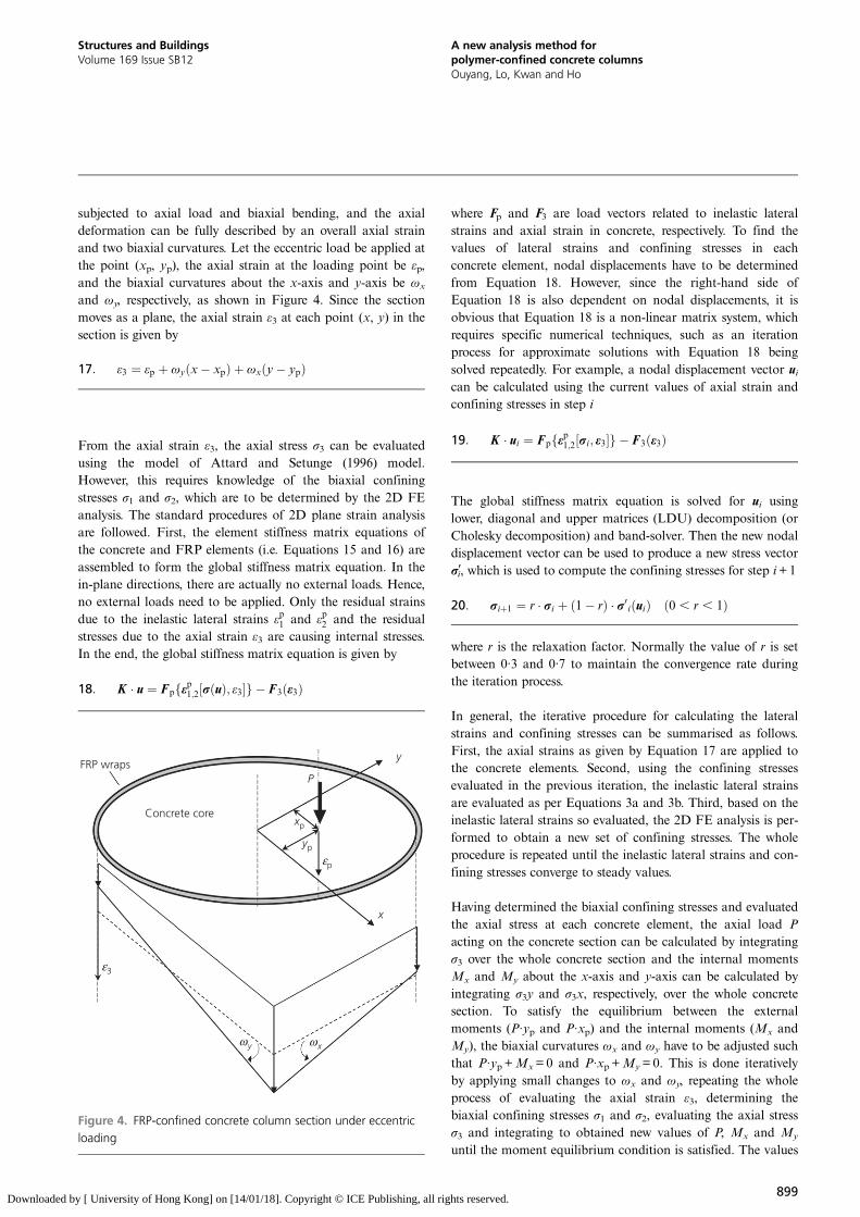
2011) in which the non-uniform stress distributions are mod-elled in the form of parallel strips and the confining stresseswithin a single strip are assumed to be isotropic. However,from the present FE analysis (which should be more rigorous)it was observed that, under eccentric loading, the stress distri-butions are not in the form of parallel strips and the confiningstresses are not isotropic, as shown in Figure 11. Moreover, toillustrate the distributions of axial stress over the cross-section,numerical results of the one-ply and the two-ply specimenswith de = 10 mm and de = 50 mm when the displacement at theloading point is equal to 3·0 mm are plotted in Figure 12. Allthese results were achieved by FE analysis using the 6718-element mesh.

When de = 10 mm, most of the concrete sections for both theone-ply and the two-ply specimens are subjected to σ1 greaterthan 2·5 MPa at a displacement of 3·0 mm, as shown inFigures 11(a) and 11(b). In the same sections, the areas with σ2greater than 2·5 MPa are slightly smaller than those of σ2,as shown in Figures 11(c) and 11(d). It can be observedthat, although the boundaries of different domains of stressesare irregular, the pattern of distribution is presented bydefinite layers of different colours, which is following the trendthat the areas with higher axial compression normally possesslarger values of σ1 and σ2. An exception was found inFigure 11(b), with σ1 built up at the top zone of the half circu-lar section.

Figures 12(a) and 12(b) illustrate that more than half of theconcrete sections of the one-ply and the two-ply specimenswith de = 10 mm were subjected to an axial stress (i.e. σ3greater than 1·2fc (36·1 MPa)). Although the distribution pat-terns of the stresses for these two cases are similar, it is very

–0·01

0

0·01

0·02

0·03

0·04

0·05

0·06

0·07

0·08

0 0·05 0·10 0·15 0·20 0·25 0·30 0·35

PD%

One-ply Two-ply

de/D

Figure 10. Percentage difference between the two meshes of

2203 and 6718 elements for one-ply and two-ply specimens

905




obvious that the magnitudes of the stresses in the two-plysection are significantly larger than those in the one-plycounterpart. However, for the cases of de = 50 mm displayed inFigures 12(c) and 12(d), both the distributions and magnitudesof σ3 in the two sections bear decent resemblance, and theareas with σ3 > 36·1 MPa are all localised to the most compres-sive ends of the sections.

It was mentioned in Section 2.3 that the effective value of fr isdetermined by fr =min{σ1, σ2}; the variations of fr along withthe displacement at the loading point for two-ply specimenswith de = 10 mm and 50 mm are shown in Figure 13. Themagnitudes of fr keep increasing as the displacement grows,and their distribution patterns are similar to those displayed inFigures 11 and 12, but with more regular curved boundariesbetween layers of different colours.

To further study how the confining stresses vary with theeccentricity, the average confining stress fr,avg was determined as

23: fr;avg ¼Pn

i¼1ð fr;i�AiÞAc

where n is the total number of concrete elements, Ai is the areaof the element i and Ac is the total area of the concretesection. The average confining stress so determined at eachloading step is plotted against the displacement for the differ-ent specimens with different eccentricities in Figure 14. It isobvious from the figure that the average confining stressincreases as the displacement increases but its value is gener-ally lower at a larger eccentricity. This also means that in thedesign of FRP-confined columns under eccentric loading,thicker FRP wraps have to be used to attain the same level of

Min 0·5 2·5 4·5 6·5 8·5 10·5 Maxσ1: MPa:

80

60

y: m

m

x: mm(a)

40

20

0–80 –60 –40 –20 0 20 40 60 80

Min 0·5 2·5 4·5 6·5 8·5 10·5 Maxσ1: MPa:

80

60

y: m

mx: mm

(b)

40

20

0–80 –60 –40 –20 0 20 40 60 80

Min 0·5 2·5 4·5 6·5 8·5 10·5 Maxσ2: MPa:

80

60

y: m

m

x: mm(c)

40

20

0–80 –60 –40 –20 0 20 40 60 80

Min 0·5 2·5 4·5 6·5 8·5 10·5 Maxσ2: MPa:

80

60

y: m

m

x: mm(d)

40

20

0–80 –60 –40 –20 0 20 40 60 80

Figure 11. Distributions of (a) σ1 (one-ply), (b) σ1 (two-ply),

(c) σ2 (one-ply) and (d) σ2 (two-ply) specimens with de = 10 mm

(displacement at loading point = 3·0 mm)

906




confinement at larger eccentricity. Another important obser-vation is that one more layer of FRP will let the value of fr,avgincrease from 4·2 MPa to 6·5 MPa at a displacement of3·0 mm for specimens under concentric loading, whereas thereis not much of a difference (2·4 MPa for one-ply and 2·6 MPafor two-ply) for specimens with de = 40 mm. In other words,FRP wraps are less effective under eccentric loading than con-centric loading.

5. ConclusionsIn order to evaluate non-uniform and anisotropic confiningstresses in confined concrete and study the full-range non-linear behaviour of confined concrete columns, a new FEanalysis method was developed by integrating the lateralstrain–axial strain model of Dong et al. (2015a), the triaxialfailure surface of Menétrey and Willam (1995), the axialstress–strain model of Attard and Setunge (1996) and thestrain gradient model developed by Ho and Peng (2013) and

treating the analysis of the biaxial confining stresses in the con-crete section as a 2D analysis problem. In theory, the new FEanalysis method should be applicable to confined concretecolumns of any shape and under any combination of axialload and bending moment, but, as a start, it was applied inthis paper only to FRP-confined concrete columns of circularshape and under eccentric loading.

To verify the applicability and accuracy of the newly developedFE analysis method, 22 specimens of FRP-confined circularconcrete columns tested under eccentric loading by Wu andJiang (2013) were analysed and two sets of numerical resultsobtained by the FE analysis implementing different meshes (a2203-element mesh and a 6718-element mesh) were comparedwith the corresponding experimental results. It was found thata high-density mesh is necessary when a large eccentricity ispresent in the load case due to the concentration of strains andstresses over the section. Overall, the loads predicted by the

Min 36·1 43·3 50·6 57·8 65·0 72·2 Maxσ3: MPa:

80

60

y: m

m

x: mm(a)

40

20

0–80 –60 –40 –20 0 20 40 60 80

Min 36·1 43·3 50·6 57·8 65·0 72·2 Maxσ3: MPa:

80

60

y: m

m

x: mm

(c)

40

20

0–80 –60 –40 –20 0 20 40 60 80

Min 36·1 43·3 50·6 57·8 65·0 72·2 Maxσ3: MPa:

80

60

y: m

m

x: mm(d)

40

20

0–80 –60 –40 –20 0 20 40 60 80

Min 36·1 43·3 50·6 57·8 65·0 72·2 Maxσ3: MPa:

80

60

y: m

m

x: mm

(b)

40

20

0–80 –60 –40 –20 0 20 40 60 80

Figure 12. Distribution of σ3: (a) de = 10 mm, one-ply;

(b) de = 10 mm, two-ply; (c) de = 50 mm, one-ply; (d) de = 50 mm,

two-ply (displacement at loading point = 3·0 mm)

907




FE analysis agreed quite well with the experimental results, therespective mean values for PFE-I/Ptest and PFE-II/Ptest equal to0·90 and 0·88 and corresponding coefficients of variance equalto 7·1% and 7·7%.

The FE analysis results revealed that, for FRP-confined circu-lar concrete columns under eccentric loading, the confiningstresses are far from being uniform or isotropic. Hence, thepreviously developed formulas and models for evaluation of

confining stresses, which assume that the confining stresses areuniform and isotropic, are not generally applicable. Moreover,the axial stress distribution is very different from the axialstrain distribution and therefore has to be analysed as an inte-gral part of the theoretical analysis. Lastly, the FE results alsorevealed that the average confining stress in the sectiondecreases as the eccentricity of the loading increases. Hence,FRP wraps are less effective under eccentric loading than con-centric loading.

Min 0·5 2·5 4·5 6·5 8·5 10·5 Maxfr: MPa:

80

60

y: m

m

x: mm

(a)

40

20

0–80 –60 –40 –20 0 20 40 60 80

Min 0·5 2·5 4·5 6·5 8·5 10·5 Maxfr: MPa:

80

60

y: m

m

x: mm

(b)

40

20

0–80 –60 –40 –20 0 20 40 60 80

Min 0·5 2·5 4·5 6·5 8·5 10·5 Maxfr: MPa:

80

60

y: m

m

x: mm

(c)

40

20

0–80 –60 –40 –20 0 20 40 60 80

Min 0·5 2·5 4·5 6·5 8·5 10·5 Maxfr: MPa:

80

60

y: m

m

x: mm

(d)

40

20

0–80 –60 –40 –20 0 20 40 60 80

Min 0·5 2·5 4·5 6·5 8·5 10·5 Maxfr: MPa:

80

60

y: m

m

x: mm

(e)

40

20

0–80 –60 –40 –20 0 20 40 60 80

Min 0·5 2·5 4·5 6·5 8·5 10·5 Maxfr: MPa:

80

60

y: m

m

x: mm

(f)

40

20

0–80 –60 –40 –20 0 20 40 60 80

Figure 13. Variation of fr for two-ply specimens:

(a) de = 10 mm and (b) de = 50 mm with displacement at loading

point = 0·75 mm; (c) de = 10 mm and (d) de = 50 mm with

displacement at loading point = 1·5 mm; (e) de = 10 mm and

(f) de = 50 mm with displacement at loading point = 2·25 mm;

(g) de = 10 mm and (h) de = 50 mm with displacement at loading

point = 3·0 mm (continued on next page)

908




Min 0·5 2·5 4·5 6·5 8·5 10·5 Maxfr: MPa:

80

60

y: m

m

x: mm(g)

40

20

0–80 –60 –40 –20 0 20 40 60 80

Min 0·5 2·5 4·5 6·5 8·5 10·5 Maxfr: MPa:

80

60

y: m

m

x: mm

(h)

40

20

0–80 –60 –40 –20 0 20 40 60 80

Figure 13. Continued

0

1

2

3

4

5

6

7

8

0 1 2 3

(a)

(b)

4 5 6

Ave

rage

con

finin

g st

ress

: MPa

Ave

rage

con

finin

g st

ress

: MPa


A1E0 and B1E0

A1E10 and B1E10

A1E20 and B1E20

A1E30 and B1E30

A1E40 and B1E40

B1E50

0

2

4

6

8

10

12

14

16

0 1 2 3 4 5 6 7 8 9


A2E0 and B2E0

A2E10 and B2E10

A2E20 and B2E20

A2E30 and B2E30

A2E40 and B2E40

B2E50

Figure 14. Relationship between average confining stress and

load eccentricity

909




REFERENCES

Attard MM and Setunge S (1996) Stress–strain relationship ofconfined and unconfined concrete. ACI Materials Journal93(5): 432–441.

Carrasquillo RL, Slate FO and Nilson AH (1981) Properties ofhigh-strength concrete subject to short-term loads. ACIJournal 78(3): 171–178.

Chen MT and Ho JCM (2015) Concurrent flexural strength andductility design of RC beams via strain-gradient-dependentconcrete stress–strain curve. The Structural Design of Talland Special Buildings 24(9): 629–652.

Dong CX, Kwan AKH and Ho JCM (2015a) A constitutive modelfor predicting the lateral strain of confined concrete.Engineering Structures 91: 155–166.

Dong CX, Kwan AKH and Ho JCM (2015b) Effects of confiningstiffness and rupture strain on performance of FRPconfined concrete. Engineering Structures 97: 1–14.

Fam AZ and Rizkalla SH (2001) Confinement model foraxially loaded concrete confined by circular fiber-reinforced polymer tubes. ACI Structural Journal98(4): 451–461.

Harries KA and Kharel G (2002) Behavior and modeling ofconcrete subject to variable confining pressure. ACIMaterials Journal 99(2): 180–189.

Ho JCM and Peng J (2013) Strain-gradient-dependent stress–strain curve for normal-strength concrete. Advances inStructural Engineering 16(11): 1911–1930.

Ho JCM, Kwan AKH and Pam HJ (2003) Theoretical analysis ofpost-peak flexural behavior of normal- and high-strengthconcrete beams. The Structural Design of Tall and SpecialBuildings 12(2): 109–125.

Ho JCM, Lam JYK and Kwan AKH (2010) Effectiveness ofadding confinement for ductility improvement of high-strength concrete columns. Engineering Structures 32(3):714–725.

Hu B (2013) An improved criterion for sufficiently/insufficientlyFRP-confined concrete derived from ultimate axial stress.Engineering Structures 46: 431–446.

Hu B, Wang JG and Li GQ (2011) Numerical simulation andstrength models of FRP-wrapped reinforced concretecolumns under eccentric loading. Construction andBuilding Materials 25(5): 2751–2763.

Hu HT, Huang CS, Wu MH and Wu WM (2003) Nonlinearanalysis of axially loaded concrete-filled tube columns withconfinement effect. Journal of Structural Engineering,ASCE 129(10): 1322–1329.

Imran I and Pantazopoulou SJ (1996) Experimental study ofplain concrete under triaxial stress. ACI Materials Journal93(6): 589–601.

Jiang T and Teng JG (2007) Analysis-oriented stress–strainmodels for FRP-confined concrete. Engineering Structures29(11): 2968–2986.

Kwan AKH, Dong CX and Ho JCM (2015) Axial and lateralstress–strain model for FRP confined concrete. EngineeringStructures 99: 285–295.

Kwan KH and Liauw TC (1985) Computerized ultimate strengthanalysis of reinforced concrete sections subjected to axialcompression and biaxial bending. The Structural Engineer21(6): 1119–1127.

Lam L and Teng JG (2002) Strength models for fiber-reinforcedplastic-confined concrete. Journal of StructuralEngineering, ASCE 128(5): 612–623.

Lee SH, Uy B, Kim SH, Choi YH and Choi SM (2011) Behavior ofhigh-strength circular concrete-filled steel tubular (CFST)column under eccentric loading. Journal of ConstructionalSteel Research 67(1): 1–13.

Liang QQ and Fragomeni S (2010) Nonlinear analysis ofcircular concrete-filled steel tubular short columns undereccentric loading. Journal of Constructional Steel Research66(2): 159–169.

Liang QQ (2011) High strength circular concrete-filled steeltubular slender beam-columns, part I: numerical analysis.Journal of Constructional Steel Research 67(2): 164–171.

Lo SH, Kwan AKH, Ouyang Y and Ho JCM (2015) Finite elementanalysis of axially loaded FRP-confined rectangularconcrete columns. Engineering Structures 100(1): 253–263.

Mander JB, Priestly JN and Park R (1988) Theoretical stress–strain model for confined concrete. Journal of StructuralEngineering, ASCE 114(8): 1804–1826.

Menétrey P and Willam KJ (1995) Triaxial failure criterion forconcrete and its generalization. ACI Structural Journal92(3): 311–318.

Mirmiran A and Shahawy M (1997) Dilation characteristics ofconfined concrete. Mechanics of Cohesive-FrictionalMaterials 2(3): 237–249.

Mirmiran A, Zagers K and Yuan WQ (2000) Nonlinear finiteelement modeling of concrete confined by fiber composites.Finite Elements in Analysis and Design 35: 79–96.

Ozbakkaloglu T, Lim JC and Vincent T (2013) FRP-confinedconcrete in circular sections: review and assessment ofstress–strain models. Engineering Structures 49: 1068–1088.

Papanikolaou VK and Kappos AJ (2007) Confinement-sensitiveplasticity constitutive model for concrete in triaxialcompression. International Journal of Solids and Structures44(21): 7021–7048.

Popovics S (1973) Numerical approach to the complete stress–strain relation for concrete. Cement and Concrete Research3(5): 583–599.

Saadatmanesh H, Ehsani MR and Li MW (1994) Strength andductility of concrete columns externally confined with fibercomposite straps. ACI Structural Journal 94(1): 434–447.

Saenz LP (1964) Discussion of ‘Equation for the stress–straincurve of concrete’ by P. Desayi, and S. Krishnan. ACIJournal 61(9): 1229–1235.

Tao Z, Wang ZB and Yu Q (2013) Finite element modelling ofconcrete-filled steel stub columns under axial compression.Journal of Constructional Steel Research 89: 121–131.

Teng JG and Lam L (2004) Behavior and modeling of fiberreinforced polymer-confined concrete. Journal of StructuralEngineering, ASCE 130(11): 1713–1723.

910




Teng JG, Huang YL, Lam L and Ye LP (2007) Theoretical modelfor fiber reinforced polymer-confined concrete. Journal ofComposites for Construction, ASCE 11(2): 202–210.

Wu YF and Jiang C (2013) Effect of load eccentricity on thestress–strain relationship of FRP-confined concretecolumns. Composite Structures 98: 228–241.

Yu T, Teng JG, Wong YL and Dong SL (2010a) Finite elementmodeling of confined concrete-I: Drucker–Prager typeplasticity model. Engineering Structures 32(3): 665–679.

Yu T, Teng JG, Wong YL and Dong SL (2010b) Finite elementmodeling of confined concrete-II: plastic-damage model.Engineering Structures 32(3): 680–691.

HOW CAN YOU CONTRIBUTE?

To discuss this paper, please email up to 500 words to theeditor at [email protected]. Your contribution will beforwarded to the author(s) for a reply and, if consideredappropriate by the editorial board, it will be published asdiscussion in a future issue of the journal.

Proceedings journals rely entirely on contributions fromthe civil engineering profession (and allied disciplines).Information about how to submit your paper onlineis available at www.icevirtuallibrary.com/page/authors,where you will also find detailed author guidelines.

911




A new analysis method for polymer-confined concrete columns

Documents

Transcript of A new analysis method for polymer-confined concrete columns