UNIVERSIDAD POLITÉCNICA DE MADRID

ESCUELA TÉCNICA SUPERIOR DE INGENIERÍA DE SISTEMASINFORMÁTICOS

GRADO EN INGENIERÍA DE SOFTWARE

TRABAJO DE FIN DE GRADO

A NEURAL NETWORKS BENCHMARK FOR IMAGECLASSIFICATION

Autor: Guillermo Echegoyen Blanco.

Dirigido por: Javier de Lope Asiaín

Julio 2017

brought to you by COREView metadata, citation and similar papers at core.ac.uk

provided by Servicio de Coordinación de Bibliotecas de la Universidad Politécnica de Madrid

A través de este documento, el lector puede hacerse hacerse una idea de como ha sido la historia de los métodos usadospara clasificación de imagen, tanto con métodos clásicos como con redes neuronales artificiales; todo ello en el contexto devisión para robots. Primero revisaremos los métodos clásicos, pasando por sus restricciones y limitaciones, escogeremosuno y sacaremos diferentes medidas sobre cómo se comporta. Después, exploraremos, brevemente, los tipos de redesneuronales que se utilizan para esta tarea, pasando por el estado del arte y su aportación; también escogeremos una red ymediremos su eficacia. Con todo ello, explicaremos el método empleado para medir y los resultados experimentalesobtenidos. Por último discutiremos estos resultados y expondremos nuestras conclusiones, así como posibles lineas futurasde investigación.

Through this document, the reader can get an idea of the history of modern and classic methods for the task of imageclassification, we present a simple image classification task, in the context of robotic vision, and how different neuralnetworks reach to stable solutions. First, we'll review different classic methods, evaluating their constraints and limitations,only to pick one up and benchmark it. Then, briefly, we will explore more modern methods, choose one, and benchmark it.Then, both benchmarks will be compared, and experimental results will be analyzed and explained. We'll conclude with adiscussion of the results, pointing out future lines of research.

3

3

3

4

5

5

6

7

7

8

10

10

11

12

13

13

14

14

15

16

16

17

18

19

20

20

21

23

23

25

28

28

31

33

34

35

37

38

Table of Contents

1 Introduction

1.1 Context and Motivation

1.2 Goals

1.3 Contents of this Report

2 State of the Art

2.1 Neural Networks

2.2 Why Neural Networks?

2.3 Deep Neural Networks

2.4 Convolutional Neural Networks

2.5 Residual Neural Networks

3 Neural Networks with Classic Methods

3.1 Classic Methods for Image Classification

3.2 Optimization

3.3 Used Method for the Benchmark

4 Neural Networks with Modern Methods

4.1 Modern Networks for Image Classification

4.2 Why Convolutional Networks?

4.3 Common Convolutional Network Architectures

4.4 Used Method for the Benchmark

5 Design of the Experiment

5.1 Environment

5.2 Landmarks

5.3 Datasets

5.5 Overfitting

5.4 Measures

5.7 Algorithm

5.8 Features

6 Design of the Classifiers

6.1 K-NN

6.2 Convolutional Network

7 Experimental Results

7.1 Results

7.2 Comparison

8 Conclusions and Further Work

9 Index of Figures

10 References

Appendix 1: Technological Environment (Software & Hardware)

Appendix 2: Resources and Code

Table of Contents 1

2 Table of Contents

1 Introduction

In this work we present a simple image classification task, in the context of robotic vision, and how

different neural networks reach to stable solutions. First, we'll review different classic methods, evaluating

their constraints and limitations, only to pick one up and benchmark it. Then, briefly, we will explore more

modern methods, choose one, and benchmark it. Then, both benchmarks will be compared, and

experimental results will be analyzed and explained. We'll conclude with a discussion of the results,

pointing out future lines of research.

1.1 Context and Motivation

Computer Vision (CV) is a continuously developing field, with applications in a broad range of scientific

and everyday life problems, from face recognition in social networks to homeland security. Recent years

have seen vertiginous progress; nowadays, the most advanced techniques are able to classify multiple

objects in real time streaming video, adjusting perspective, color and brightness enhacement, and virtual

rotation. CV, then, deals with the process of perceiving image and video. Perception is not only a matter

of reception of images, but comprises multiple and interrelated subroutines. All those subroutines that are

involved in the act of perception must be addressed when programming CV, and, more often than not, will

be inspired by biology [1].

The story of CV is short, as it started in the 60's, with the invention of the perceptron (Rosenblatt, 1962 [2]

). A perceptron is, roughly speaking, a simple linear classifier. Similarly to a transistor, a perceptron gives,

for a particular input, a binary output. Thus, it can be used to generate simple silogisms, as a logic gate,

or, more abstractly, to classify one dimensional problems, which is a kind of binary feature extraction.

Feature extraction is a major issue in CV. The invention was a revolution until the 70's, in which computer

science served to other, more "complicated" problems, not solved yet by neural networks. At that time,

only the perceptron was available, with manifest pitfalls. Logic problems of the form NOR (relatively

simple as an abstract problem) are out of scope of a one-layer perceptron. It is not linearly divisible, thus,

at first sight, it couldn't be solved with the neural networks of the time. In the 80's, the field was reborn

with the appearance of more intrincate and sophisticated architectures (multilayer, convolutional networks,

tree networks, etc) and learning rules. Emergent memory processes and feature extraction and match

were studied [3], until now, where CV modules are able to identify objects in different, changing

environments and perspectives, in lack of good visibility conditions, with astonishing accuracy, and in real

time.

1.2 Goals

The motivation behind this work is to find a way of dealing with the vast amount of methods relevant to the

task of Robotic Vision and finding the ones that work best. In the process we'll explore the common,

shared basis of all these methods trying to get some insights for future elections of one method or

Introduction 3

another, based on the task at hand. This will be useful for researchers as it alleviates the decision process

needed when researching higher levels of abstraction that depends on Robotic Vision, making them able

to forget about the technical issues and focusing on higher level subjects.

All in all, the benchmark proposed in this study wants to be plausible and realistic with nowaday's robotics'

constraints. Thus, some conditions must be taken into account when assessing the different

methodologies studied. For example, as a CV module installed in a robot must work "on the fly", real-time

processing will be an important issue to be evaluated. In the section dedicated to the method, all the

criteria will be explained in detail.

Therefore, the primary goal of this report is to compare classic and modern approaches to solve the task

of image classification, in an attempt to grasp some intuition over.

To address this goal, we'll present a benchmark comparing classic methods with modern networks

methods, both solving the problem of image classification in the context of robot vision. As benchmarking

all the existing methods could be nearly impossible due to the number of procedures in the field, here we'll

review some of the most representative ones, from classical, well-established methods to more modern

approaches.

Aside from the benchmark itself, this report aims to outline the evolution of the techniques utilized to solve

the problem of image classification, trying to evaluate pros and cons of every method.

1.3 Contents of this Report

In this report we state a clue on which method to choose for the task of image classification. In chapter 2

we expose the state of the art. In chapters 3 and 4 we briefly explore the history of image classification

tasks and some of the most used methods, reviewing both classic, raw statistical methods and more

modern artificial-network-oriented methods, going through it's contributions, constraints and pitfalls. Two

experiments are proposed to test each method in chapter 5. In chapter 6 we explain both methods used

and it's peculiarities, we continue explaining how the tests were conducted and the results obtained in

chapter 7 to end up with the obtained conclusions and further lines of work in the last chapter. Appendixes

1 and 2 contains the gory details about software, hardware and source code.

4 Introduction

2 State of the Art

This chapter will explore the state of the art on the subject of image classification with neural networks.

We will explore the most modern and stable methods using neural networks and finish with the latest

approaches being developed nowadays.

2.1 Neural Networks

A neural network is a computing system inspired by the biological neural networks that constitute animal

brains. Such systems learn over time to do concrete and general-purpose tasks. Artificial Neural Networks

(ANN) are composed of neurons and links. Neurons are simple imitations of biological neurons, with axes

and dendrites, the building block or ANN. Links act as synapses between neurons, connecting them, and

transportating the signal from one neuron to a given number of other neurons. Neurons receive a fixed

number of weighted inputs from other neurons. An activation function operates with the input as argument,

producing an output to be propagated. This is the most general case, but things can be much more

complicated. Weights can be binary or discrete (generally in a range between 0 and 1), and act as a way

to ponderate the importance of every neuron in the other's behavior. The activation function can be of any

mathematical nature, and, depending on the task, some are preferred over other ones. In classical

formulations, the activation function could be a binary clasificator, a threshold. If the weighted sum of

inputs reach a fixed value, the neuron would "fire", being this firing 0 or 1 (step function). More modern

formulations include logarithmic compressions, non-linear functions, and discrete (or continuous) inputs

and outputs, that opens the possibility of much more complex tasks to be resolved.

Neurons are connected in layers, and activation propagates (or not) from one neuron to another, through

the entire network (or the point where activation stops). Almost every modern ANN is composed of an

input layer receiving the information to be processed, a number of hidden layers, and an ouput layer.

Figure Fig. 1.3.1 represents schematically this notion. The number of hidden layers is also decisive in the

complexity of task accesible to the ANN, and major advances in the field come from research in the

number and nature of hidden layers and its effects on the output of the system [4], [5] , [6]. It is remarkable

that, as the number of hidden layer increase, our understanding of the final output and our capability to

predict it decrease dramatically. Input, hidden and output layers can be connected in many fashions, that

will, also, determine the performance of the network on different tasks. The final result of any input

propagated through the network will depend on the pattern of connections in every layer, the functions

governing neuronal activation and the weights fixed for each link between neurons. The structure (pattern

of connections) and the activation function play a decisive role in the final result offered by the network;

basically determine the global model of the network, that has to be in agreement with the nature of the

task to be accomplished. The model refers to the general operations carried out over the input data to

generate the output. Weights determine the parameters of the global model implemented by means of

structure and activation functions. From this can be followed that, modifying the weights, the output of the

model will vary. This is the key to learning rules, as the classical and still prevailling Hebb's Rule. Hebb's

rule and its variations are based on the principle that little adjustments in the network's weights will lead to

a stable, global solution to the problem. Its application is iterative: in each iteration, ANN's output is

State of the Art 5

compared to the desired output (target output), and the difference between them calculated. Then,

weights are slightly modified, and, if the difference is reduced in the next iteration, the change is kept and

repeated, until the real output fits the desired output to a fixed threshold (the maximum accepted error).

The ratio of modification per iteration, or learning rate (η) can be set to any value, and determines the

speed of learning. Its classic formulation is: Δw = ηx y. The change in the th synaptic weight w equals

the learning rate η times the th input x times the postsynaptic response y [3].

The input could be, as in the present work, a stream of video or a set of images. Nevertheless, almost

every piece of information can be represented in a suitable form to fit ANN requirements. Thus, ANN could

perform statistical analysis over any given data; for example, linear regressions over healthy habits

questionnaires, or Principal Component Analysis over cosmic microwave radiation data.

In our case, the input will be a set of pictures, and the general model must perform the task of image

classification. The output is precisely the classification. Various models will be tested to inform about their

performance.

Figure 1.3.1. - An Artificial Neural Network with one hidden layer

To sum up, a neural network can be though of as a conjunction of mathematical operations, usually in the

fashion of linear algebra, composed or neurons arranged in layers, and synapses connecting them. It is

usually implemented as matrix multiplication operations. This gives us the ability to model many problems,

from linear, simple equations to complex, differential equations with many parameters.

2.2 Why Neural Networks?

Neural Networks are task-nonspecific, meaning that, depending on how the problem is modelled, a wide

variety of problems can be solved. After categorizing the problem's solutions we can choose between

many types of networks, and start testing its performance. Iteratively, weights are adjusted until the

solution is stable and accurate enough, and the network can be applied not only to the problem for which it

was trained, but also to other analogous tasks. The key feature to keep in mind is that many of the

problems we can think of can be expressed in a mathematical way. This is precisely what neural network

do best.

i i i i

i i

6 State of the Art

2.3 Deep Neural Networks

Deep Neural Networks are one of the many types of neural networks. It's main difference with other

networks strives in the amount of hidden layers. Every architecture with more than one layer is considered

as deep. It first appeared in [7], where a deep, multi layer perceptron was explored to overcome the

problems of the original Rosenblatt's multilayer perceptron. It supposed a revolution in the field, and open

the door to real-world complex problems never addressed before by neural networks.

At that time, training networks iteratively was a problem, because computation resources were very

limited and no mathematical method was known to work fast and efficiently. In 1989, LeCun et al.

successfully applied the backpropagation algorithm (made popular by [8]) to the problem of recognizing

handwritten ZIP codes. It took over 3 days to fully train the network [9].

With the develop of better methods (backprop), what was left was the computational cost of the learning

process. Nowadays, with modern processors the problem is rapidly fading out. Some authors like Coates

et al. [10] explored the use of GPUs over standard processors to train networks, resulting in much more

powerful computation capabilities, that conform the standard in modern days.

2.4 Convolutional Neural Networks

A convolution is a mathematical operation that combines two functions to form a third one, it does so by

"sliding" one function over the other and multiplying the points that overlap, it is similar to cross-

correlation. Common applications are Digital Signal Processors, which are the core of audio systems or

Image Processing. Applied to our field of image classification we can think of image as two dimensional

functions (we represent images as two dimensional matrices) and we can convolve the image with a small

function that we call "kernel". To convolve, we slide the kernel to every position of the image computing a

new pixel as the weighted sum of the pixels the kernel is floating over. A visual representation can be

found in Fig. 1.3.2

This kind of procedure makes a lot of sense when thinking about images features, for example, we have

explained before that adjacent pixels keep some correlation. With convolutions this correlation is captured

as the kernel slides over the pixels, the amount of adjacency can be regulated with the size parameter of

the kernel.

State of the Art 7

Figure 1.3.2. - A kernel convolution over an image.

One great side effect of this setup is that neurons are only connected locally, conforming regions or

groups (often called patches). This saves us from a very big weight matrix, which in turn alleviates the

computation process and helps scaling the architecture.

2.5 Residual Neural Networks

It has been stated that depth plays a big role in deep networks [5] , [6] , but as depth grows difficult in

training does so too, as well as overfitting. This happens because of the training techniques used, usually

SGD (Stochastic Gradient Descent) and the random initialization of the network [4].

To overcome this problem many techniques have been explored. [11] and [12] tried to initialize the

network normalized while [12] introduced intermediate normalization layers. Both methods seem to work

well for very deep networks but it comes at a cost: as the network starts converging to a stable solution,

accuracy saturates and then degrades very fast [13], [14].

In the last decade of the past century, [15] and [16] proposed a technique for connecting layers called

shortcut connections, illustrated in Fig. 1.3.3. It works by connecting layers skipping one or two other

layers in between, giving a sense of fast forwarding knowledge.

Figure 1.3.3. - A shortcut connection between two layers

In [4] they bring the concept back again and use it to solve this degradation problem with amazing results,

8 State of the Art

so much that it served to win the ILSVRC 2015 & COCO 2015 competitions, which are the most important

contests of image classification and segmentation.

Networks setup with shortcut connections are what we call Residual Networks, the key of this mechanism

is it's ability to recover previously stored knowledge that is fading out (degrading accuracy) by bypassing

the units causing that fade and forwarding that knowledge, then it is restored with backpropagation to the

conflicting units.

State of the Art 9

3 Neural Networks with Classic Methods

In the following chapter we'll review the most common, classic methods utilized in the past years to solve

image classification tasks. Feature extraction and classification will be presented, as well as a standard

optimization procedure. At last, a classical method to benchmark will be proposed.

3.1 Classic Methods for Image Classification

The problem of classification has been a tough nut to crack since the beginnings of computer science.

The first approaches were based on raw statistical methods, suitable for different kinds of classifications.

Linear Classifiers appeared first, comprising techniques like LDA (Linear Discriminant Analysis) [17],

Logistic Regression, Naive Bayes Classifiers or the well known Perceptron proposed by Rosenblatt back

in 1962 [2] ). Later, in 1995 the SVM (Support Vector Machines) appeared [18], which can be though of as

a small network (see below).

Feature Extraction

Image classification has been a subject of study for a while. As soon as 1973, Haralick et al. [19] explored

the task by extracting basic features from images with statistical methods. Images are worked out as

matrices of pixels to operate upon, just like nowadays. In their method they state what an important

characteristic must have to be considered classifiable and then propose various characteristics that can

be found in any image and the methods to extract them. Amongst other features, they propose measures

of correlation between pixels and entropy.

Along these lines of study, different methods started to appear: points of interest tracking [20] in 1981,

improvements over corner detection [21] in 1988, motion recovery (1992) [22] and features detection with

a moving correlation window [23] in 1995. All these methods share the same working principle: find

characteristic, important features in the most invariant and robust way and work on those features. All of

them work with correlations between pixels and gradients made out of these pixels, in the same picture,

or along a succession of pictures. In this sense, statistical measures like gradients analysis and

correlation have played a central role.

Following these statistical measures we reach to the Scale Invariant Transform method (SIFT) [24], a

method to extract features from images that can be invariant to image scale and rotation, this method is

powerful, but at the time it was slow to compute. Ke and Sukthankar used PCA to normalize gradient

patch instead of histograms [25] and showed that PCA-based descriptors can also be distinctive and

robust to image deformations. Later on, in 2006, the Speed Up Robust Features method was proposed

[26], being speed one if its selling point against SIFT and PCA-based descriptors.

10 Neural Networks with Classic Methods

Feature Classification

In [27],a decision technique called K-Nearest Neighbour (K-NN) is explored. Basically, K-NN assigns to an

unclassified item the class most heavily represented among its k nearest neighbours, to do this, during

training we expose the classifier to different items with n features, it then creates an n − dimensional

feature space and projects the data onto it. With this feature space constructed, we can input an unknown

item with similar features and extract the distance of every neighbor to it. Although this method is slow (it

has to check the distance of every item with every other item), it is still in use in image classification as it

is easy to implement and understand.

A distinctive approach is that of Support Vector Machines (SVM), based on Fisher's pattern recognition

work [28]. Cortes et al. (1995) in [18] explored the concept creating a Support Vector Network able to

recognize handwritten digits. The core idea is to non-linearly map input vectors to a high dimensional

feature space and construct a decision linear n − dimensional divider inside this feature space. SVMs

have been widely used for more than two decades with great results in classification tasks.

3.2 Optimization

All the aforementioned methods share a common problem: the bigger the input dimension, the slower the

algorithm becomes. This is due to the fact that the features are extracted operating on the whole pixel

matrix, SIFT and SURF pre-process the image best guessing points of interest, but they are slow to

converge though. To overcome this problem, the preferred approach is input dimensionality reduction.

We'll review basic techniques to achieve this.

Speed up by Dimensionality Reduction

A first step into dimensionality reduction could be acknowledging that, in many cases we can perform the

classification over a well distinctive feature descriptor rather than over the original image itself. In this

sense we can note that in many situations, color histogram is a great descriptor, in [29] they demonstrate

it's effectiveness with an SVM.

We can reduce dimensionality even further by applying some of the revised techniques so far, being PCA

(Principal Components Analysis) or LDA (Linear Discriminant Analysis) based methods the most common.

From a classifier perspective, the details are not so important and in fact, they can represent noise. That

is why summarization techniques like these work so well.

Another commonly seen technique is to stack processing units in such a way that minimizes computation.

A great example are the Support Vector Machines, which are made of feature classifiers. Each classifier

is specialized in a certain feature, then we stack all of them ranging from more abstract to more concrete

features, this way the top classifiers (abstract) filter out non-interesting points or regions, saving time and

computation to the lower classifiers.

Neural Networks with Classic Methods 11

3.3 Used Method for the Benchmark

For our benchmark we are going to use the histogram of the images to characterize them and classify

with a K-NN. We use this technique because is a well established method to classify features over a data

set.

12 Neural Networks with Classic Methods

4 Neural Networks with Modern Methods

So far we have reviewed some classic methods for image classification, in this chapter we will do so for

the approach of modern neural networks.

In the last two decades, computers computation capabilities have been enormously increased, this fact

has made possible for us to create bast neural networks and test them. In the past, nobody could theorize

about very big networks because they were not able of test it nor computers able to run it, nowadays, we

are breaking that barrier with the usage of GPUs optimized for the task.

4.1 Modern Networks for Image Classification

In 1998 LeCun et al. [30] proposed an architecture, LeNet5 (Fig. 1.5.1) one of many previously successful

iterations of a convolutional architecture for digits recognition.

Figure 1.5.1. - LeNet5: Convolutional Neural Network for digits recognition

LeNet5 showed that as images are spatially correlated, using a multi-layer network for the input in a per-

pixel basis would not take advantage of this correlation, therefore LeNet5 uses a convolutional layer with

learnable parameters as input, which is an effective way to extract features distributed across the image

with fewer parameters.

Until the arrive of big GPUs, computation has always been a limitation factor for neural networks, but

many research has been done. Ciresan et al. proposed it's usage for MLPs (Multi Layer Perceptrons) and

managed to outperform previous results [31], but it was with [10] that GPUs established as the first choice

for neural networks computations.

With powerful performance, Alex Krizhevsky et al. managed to train a very deep network (AlexNet, Fig.

1.5.2) for the ImageNet competition, winning by far to the other competitors [32], it was based on LeNet5

but with some more insights: it uses ReLU (Rectified Linear Unit) as non-linearity (instead of tanh) and

introduced dropout and data augmentation, which are techniques to avoid overfitting.

Neural Networks with Modern Methods 13

Figure 1.5.2. - AlexNet, winner of the ImageNet 2012

There are many more important deep architectures, we will review some of them in the following sections.

4.2 Why Convolutional Networks?

There are many types of deep networks, but why use convolutions? It has been thoroughly demonstrated

that convolutions work well for the task, they are able to capture the correlation between pixels and

regions in the image as well to remember lots of different classes.

4.3 Common Convolutional Network Architectures

The most common layers in ConvNets are:

Convolution: This is the most important layer, it convolves it's input and has some learnable

parameters: kernel size, stride, zero padding and number of filters.

Non-Linearity (Usually ReLU): This layer applies a non linear function to it's input (non saturating also,

in the case of ReLU) , without this layer the hole network would be just a linear classifier.

Pool (Usually Max Pooling): This layer is used to downsample the input, this is useful to reduce the

conv layers processing overhead.

FC (Fully connected layer): This layer is a full network by itself, it is normally used as the last layer of

the ConvNet, as a classifier of the convolutional part.

A commonly seen configuration is INPUT -> [[CONV -> RELU]*N -> POOL?]*M -> [FC -> RELU]*K ->

FC , where N an M are multiplicative factors and ? implies that the layer is optional.

14 Neural Networks with Modern Methods

4.4 Used Method for the Benchmark

Training a deep network is hard, requires lots of data and a powerful computer for a long period of time,

hence instead of training our own network we are going to use a technique called transfer learning (more

on this in Comparison section) with a pretrained network. We will use Inception v3 (Google's image

classification network) with tensorflow (google's proprietary library for artificial intelligence) and Python to

retrain the last layers so that it recognizes our data.

Neural Networks with Modern Methods 15

5 Design of the Experiment

The main goal of image classification is to categorize digital images under a given criteria or a set of

possible choices. To do so, many different algorithms are available. Techniques focus on analyzing the

image as a whole, or a portion of it; then, try to assign one or various tags, based on the analysis over the

pixels. The classification step is usually a low level tool used as a background for other tasks such as

segmentation or edge detection. It is therefore intended to be a semi automated task which runs on a

given image or set of images and outputs a classification tag which might be used by upper levels of

abstraction.

A simple task of recognition could be approached as follows: first, select objects from the image by

segmenting it. To do so, scan pixel by pixel changes in brightness. When an abrupt change is detected,

select it as a contour, thus dividing pixels at both sides of the gradient change as different objects. Also,

when contours are closed, the inside of that contour can be considered an object. Then, compare the

extracted objects to a database of known objects. If the configuration of pixels (in coordinates and

brightness) of the objects extracted are under a certain, fixed threshold of variability in comparison to

those stored in memory (or a linear transormation of them), then considered both objects the same.

Many other ways exist to solve the problem of image recognition, resembling in variable degree the

human vision system. The only way to asses their efficacy is by facing them to real image classification

problems and measuring their performance.

This benchmark aims to measure different methods for image classification applied to a real world use

case: A robot moving in a environment where it knows the map and tries to go from one (start) point to

another (end) recognizing each landmark from a camera. To do it we will be using the images classified as

landmarks (split from videos) and the following methods:

Classic method: Color histogram with a K-NN classifier and opencv.

Modern method: Transfer learning with Inception v3 and tensorflow.

K-NN works by composing a search tree with the possible pre-specified classes and then matching the

input against the nearest class. The search tree is constructed during the training step, it will take as input

the color histogram of every image in the training set along with the class the image corresponds to. With

the convolutional network we will retrain the last layers of the pretrained network with our train set.

For each method we will: train, test and measure it's response time and accuracy.

5.1 Environment

To ensure the benchmark is as fair as possible with both methods we will apply the following

requirements:

Isolation: The benchmark of every method is going to run in an isolated docker container with no

other application running, this should minimize resource competition between processes.

Similar technology: Both benchmarks will be run in a custom python script. I chose python over

1

16 Design of the Experiment

other programming languages because it is easy to read and both tensorflow and opencv libraries

have bindings for it. If we were to program with different languages time-efficiency issues might be

encountered.

5.2 Landmarks

We have established various landmarks (points of the map) from the Computer Science Systems

Department (Departamento de Sistemas Informáticos) and it's insides. We have captured some videos,

split them into images and composed a map with them, we detail every one in the following chart:

# Name Description Sample

1 FloorThe floor in the just before the departments' doors. First

floor, fourth block

2 Doors

The doors to the Computer Science Systems Department

and the Economics Department, just before the corridor.

First floor, fourth block.

3 Corridor The corridor to the Computer Science Systems Department.

4 Mailboxes The mailboxes in the corridor, just before the departments.

5 Fountain The fountain at the end of the corridor, near the offices.

Design of the Experiment 17

6Bath

doorsThe bath doors at the right of the fountain.

7 Office The Bachelor's director office.

8Corridor

way backThe corridor from the other side, the way back to the floor.

# Name Description Sample

5.3 Datasets

We will divide all our images by landmark, then, for every landmark we are going to take 80% for training

and 20% for testing (these are typical numbers, not just randomly chosen), we do this to avoid testing with

the same images that we train as it would be too easy for any classifier, after all it would have yet seen the

image.

The procedure for composing the samples is not complex:

1. Take various videos of all the landmarks

2. Split the video in frames

3. Classify each frame (bunch of frames) by landmark

4. Augment samples (more on this in Overfitting section)

5. Separate frames from each landmark in trainset (80%) and testset (20%)

6. Reduce dimensionality (reduce images from 1920x1080 to 250x141 and 1080x1920 to 141x250 and

grayscale) to avoid large computation

Before the augmentation step I was able to obtain a good amount of samples, about 1000 samples

average, being 518 samples the minimal by landmark. It is worth noting that for the K-NN algorithm to

18 Design of the Experiment

work well the dataset must be well-balanced (although much implementations work this out), if the amount

of samples in a class is much bigger than in other classes, the probability that a neighbor of that class is

found get's increased. Also, as we have images in portrait and in landscape, width and height will differ,

which in turn will affect the histogram, for this reason we do not take the histogram itself but it's

normalized version.

Although for K-NN we will resize every sample to 250x141 or 141x250 in order to avoid possible

histogram pitfalls and process only in graysclae, in the case of the ConvNet this is not necessary as it

automatically rescales everything to 299x299x3, being the last x3 the number of channels, so full color

images are to be used.

To sum up we will have a dataset with the following characteristics:

Landmark No Augmentation Hflip Augmentation Balanced

Office 1464 2928 1036

Fountain 518 1036 1036

Mailbox 706 1412 1036

Doors 1560 3120 1036

Bathdoors 662 1324 1036

Back 1443 2886 1036

Corridor 798 1596 1036

Floor 969 1938 1036

5.5 Overfitting

A common problem when training is overfitting; that is basically that your model learns too well your data

and so it does not generalize correctly. We definitely do not want this to happen, to avoid this effect we

are going to augment our data, which consists in taking our data and do some transformations on it so

that the dataset grows with samples that are slightly different.

There are many techniques applicable here, we could crop the image, change the color map, zoom,

rotate or flip it. In our case we are going to augment our data by a factor of two

Also, we must estimate the best values for our models. In the case of the K-NN we have a very important

one, the number of neighbors used for predictions k, to estimate it we are going to use cross-validation

with our trainset, this will help us to prevent overfitting too as it vanishes the importance of initialization in

our trainset.

Design of the Experiment 19

5.4 Measures

Accuracy

This is the precision of each method in test. For each class we are going to take all the test images and

pass them through the classifier, obtaining a predicted class for each image, then we average that class

predictions to obtain an average accuracy for the class, we will call this average it's score. Finally we will

average the score of all classes obtaining a global score for the classifier.

Time

This is time spent by each classifier while predicting the class of each image, this will be used as a

constraint for real-time. We measure it by getting the delta time before and after the predict function call.

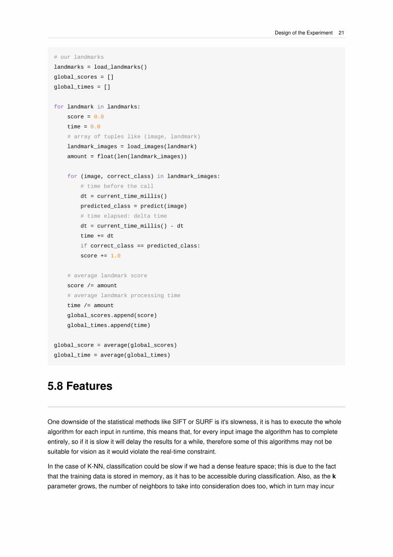
5.7 Algorithm

The algorithm in pseudo-python code can be seen down below. This procedure is done for both methods,

we will see the comparison between the scores and global score of each method as well as the times and

global time.

Whenever a prediction is done correctly (the predicted class for the image is the actual correct one) we

add one point to the score, if it fails no penalization is applied.

20 Design of the Experiment

# our landmarks

landmarks = load_landmarks()

global_scores = []

global_times = []

for landmark in landmarks:

score = 0.0

time = 0.0

# array of tuples like (image, landmark)

landmark_images = load_images(landmark)

amount = float(len(landmark_images))

for (image, correct_class) in landmark_images:

# time before the call

dt = current_time_millis()

predicted_class = predict(image)

# time elapsed: delta time

dt = current_time_millis() - dt

time += dt

if correct_class == predicted_class:

score += 1.0

# average landmark score

score /= amount

# average landmark processing time

time /= amount

global_scores.append(score)

global_times.append(time)

global_score = average(global_scores)

global_time = average(global_times)

5.8 Features

One downside of the statistical methods like SIFT or SURF is it's slowness, it is has to execute the whole

algorithm for each input in runtime, this means that, for every input image the algorithm has to complete

entirely, so if it is slow it will delay the results for a while, therefore some of this algorithms may not be

suitable for vision as it would violate the real-time constraint.

In the case of K-NN, classification could be slow if we had a dense feature space; this is due to the fact

that the training data is stored in memory, as it has to be accessible during classification. Also, as the k

parameter grows, the number of neighbors to take into consideration does too, which in turn may incur

Design of the Experiment 21

into computation delay. Our data is not dense in features nor in number, so this will probably not be an

issue.

On the other hand, neural nets are slow to train but faster in runtime, this is due to the way networks work.

When training, backpropagation is used to transmit the gradients back to the input for the parameters to

be learned, that is slow but as it is only used during training, not in normal use, it does not delay so much.

A forward pass could be slow too, depending on the number of layers and operations per layer but this is

usually been taken care of by design. However large architectures like the one we'll employ here will

always have a considerable processing overhead, only surpassable with more computation capabilities,

namely a GPU card. This is because tensorflow was designed to scale seamlessly across cpu and gpu

available in

runtime.

. Docker is a containerization technology that is able to take full cpu and memory, we will use it to

avoid installing all necessary software and instead used prepared containers that take full advantage

of our resources. ↩

1

22 Design of the Experiment

6 Design of the Classifiers

After reviewing the whole setup for the designed experiment, it is time to present each classifier and how

we are going to use each one.

6.1 K-NN

We train our classifier with supervised learning, passing through the histogram of each picture along with

it's corresponding class. This will setup the whole feature space the classifier is going to memorize . To do

so, the classifier understands each histogram as a multidimensional feature vector, to which a class label

is to be assigned; therefore the process of training consists in storing each feature vector along it's class

label. During the classification phase we ask the classifier to predict the class of each item (histogram of

every image). In order to do it, the classifier assigns the label which is most frequent among the k nearest

neighbors to the query sample. The euclidean distance is widely employed to calculate the distance of the

neighbors to the sample although other measures have been used too (Hamming distance, Pearson and

Spearman).

OpenCV's k nearest neighbor implementation uses the euclidean distance when employed for

classification (Bayes is used for regression), which is a safe choice, but not the best. The distance metric

method used can push the classification accuracy significantly, Goldberger et al. explore solutions to learn

how to reduce dimensionality before the training step and suitable distance according to the nature of the

data [33] and [34] tries to establish a reliable method for the case where the distances between neighbors

is big.

Besides the method employed for metric distance, there is another important parameter, the k neighbors

to use when classifying, in our case we will use cross validation to estimate it, the full process is reviewed

hereafter.

K Neighbors Estimation

The k neighbors parameter is of the most importance in the K-NN algorithm, it is the amount of neighbors

used for matching. We will use a type of cross validation called k-folds to estimate the best k neighbors

for our data, to do so, during training we will randomly partition the dataset into k equal sized subdatasets,

then we will train on k-1 subdatasets and validate on the remaining one, this process is repeated k-1

times more so that every subsample is used for validation only once. By measuring the error on each pass

and averaging it we obtain a more accurate error rate for the chosen k neighbor. We will repeat this

procedure for all the values of k we want to test and choose the one that minimizes the error. We pick

k − folds = 10 as it is a multiplier of the amount of samples we have on each class. The pseudo-python

algorithm showing the whole process can be seen below:

Design of the Classifiers 23

k_folds = 10

k_values = [1, 2, 3, 4, 5, 6, 7, 8, 9, 10, 11, 12, 13, 14]

error_rates = []

for k_value in k_values:

folds = get_folds(k_folds)

error = 0.0

for fold in folds:

knn.train(fold.train_set)

fold_error = 0.0

for (sample, correct_class) in fold.validation_set:

predicted_class = kn.predict(sample)

if predicted_class != correct_class:

fold_error += 1.0

fold_error /= float(len(fold.validation_set))

error += fold_error

error /= float(len(folds))

error_rates.append(error)

# best k will be the k value at the position where the error is minimal

best_k = k_values[ error_rates.index(min(error_rates)) ]

After running the cross validation I found that the setup that works best is for k = 1 (depicted in this chart),

so this is the value we will use for the benchmark.

K Error K Error

1 0.03188 8 0.08773

2 0.05156 9 0.09156

3 0.06250 10 0.09414

4 0.07102 11 0.09891

5 0.07492 12 0.10016

6 0.07992 13 0.10312

7 0.08234 14 0.10719

With the chosen value we can start the benchmark for the classic method.

24 Design of the Classifiers

6.2 Convolutional Network

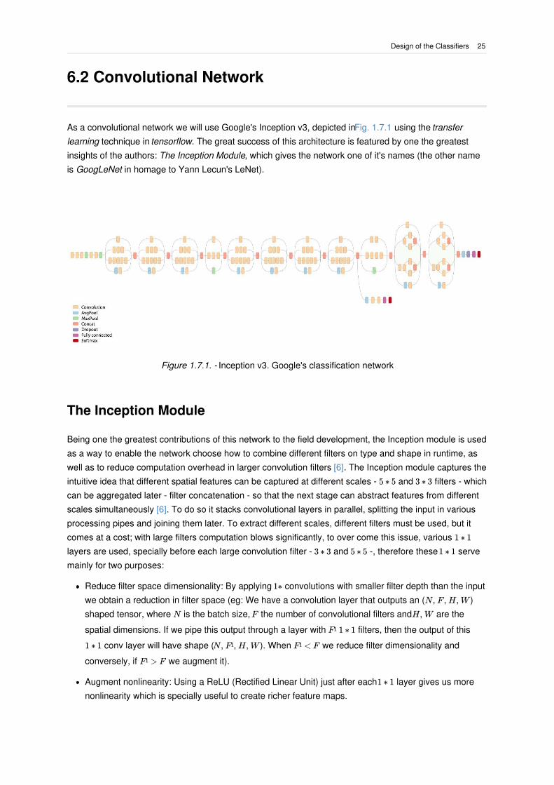
As a convolutional network we will use Google's Inception v3, depicted in Fig. 1.7.1 using the transfer

learning technique in tensorflow. The great success of this architecture is featured by one the greatest

insights of the authors: The Inception Module, which gives the network one of it's names (the other name

is GoogLeNet in homage to Yann Lecun's LeNet).

Figure 1.7.1. - Inception v3. Google's classification network

The Inception Module

Being one the greatest contributions of this network to the field development, the Inception module is used

as a way to enable the network choose how to combine different filters on type and shape in runtime, as

well as to reduce computation overhead in larger convolution filters [6]. The Inception module captures the

intuitive idea that different spatial features can be captured at different scales - 5 ∗ 5 and 3 ∗ 3 filters - which

can be aggregated later - filter concatenation - so that the next stage can abstract features from different

scales simultaneously [6]. To do so it stacks convolutional layers in parallel, splitting the input in various

processing pipes and joining them later. To extract different scales, different filters must be used, but it

comes at a cost; with large filters computation blows significantly, to over come this issue, various 1 ∗ 1

layers are used, specially before each large convolution filter - 3 ∗ 3 and 5 ∗ 5 -, therefore these 1 ∗ 1 serve

mainly for two purposes:

Reduce filter space dimensionality: By applying 1∗ convolutions with smaller filter depth than the input

we obtain a reduction in filter space (eg: We have a convolution layer that outputs an (N, F , H, W )

shaped tensor, where N is the batch size, F the number of convolutional filters and H, W are the

spatial dimensions. If we pipe this output through a layer with F 1 ∗ 1 filters, then the output of this

1 ∗ 1 conv layer will have shape (N, F , H, W ). When F < F we reduce filter dimensionality and

conversely, if F > F we augment it).

Augment nonlinearity: Using a ReLU (Rectified Linear Unit) just after each 1 ∗ 1 layer gives us more

nonlinearity which is specially useful to create richer feature maps.

1

1 1

1

Design of the Classifiers 25

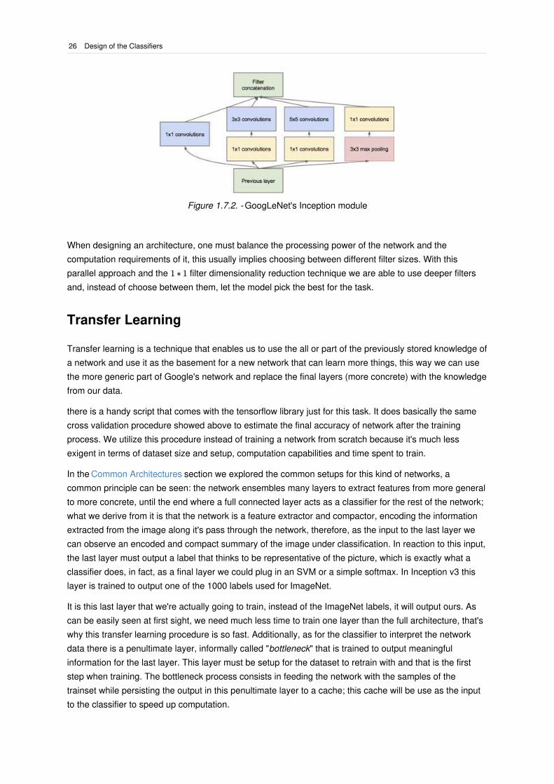
Figure 1.7.2. - GoogLeNet's Inception module

When designing an architecture, one must balance the processing power of the network and the

computation requirements of it, this usually implies choosing between different filter sizes. With this

parallel approach and the 1 ∗ 1 filter dimensionality reduction technique we are able to use deeper filters

and, instead of choose between them, let the model pick the best for the task.

Transfer Learning

Transfer learning is a technique that enables us to use the all or part of the previously stored knowledge of

a network and use it as the basement for a new network that can learn more things, this way we can use

the more generic part of Google's network and replace the final layers (more concrete) with the knowledge

from our data.

there is a handy script that comes with the tensorflow library just for this task. It does basically the same

cross validation procedure showed above to estimate the final accuracy of network after the training

process. We utilize this procedure instead of training a network from scratch because it's much less

exigent in terms of dataset size and setup, computation capabilities and time spent to train.

In the Common Architectures section we explored the common setups for this kind of networks, a

common principle can be seen: the network ensembles many layers to extract features from more general

to more concrete, until the end where a full connected layer acts as a classifier for the rest of the network;

what we derive from it is that the network is a feature extractor and compactor, encoding the information

extracted from the image along it's pass through the network, therefore, as the input to the last layer we

can observe an encoded and compact summary of the image under classification. In reaction to this input,

the last layer must output a label that thinks to be representative of the picture, which is exactly what a

classifier does, in fact, as a final layer we could plug in an SVM or a simple softmax. In Inception v3 this

layer is trained to output one of the 1000 labels used for ImageNet.

It is this last layer that we're actually going to train, instead of the ImageNet labels, it will output ours. As

can be easily seen at first sight, we need much less time to train one layer than the full architecture, that's

why this transfer learning procedure is so fast. Additionally, as for the classifier to interpret the network

data there is a penultimate layer, informally called "bottleneck" that is trained to output meaningful

information for the last layer. This layer must be setup for the dataset to retrain with and that is the first

step when training. The bottleneck process consists in feeding the network with the samples of the

trainset while persisting the output in this penultimate layer to a cache; this cache will be use as the input

to the classifier to speed up computation.

26 Design of the Classifiers

During the training phase, the testset provided is traversed extracting the bottleneck file for each image

and forwarding it to the classifier, which outputs a label that is tested against the correct label, the last

layer's weights are updated accordingly through the back-propagation algorithm.

Design of the Classifiers 27

7 Experimental Results

In this chapter we present the experimental results of the benchmark, explaining how the experiment was

conducted. Also, the methodology of each probe will be detailed.

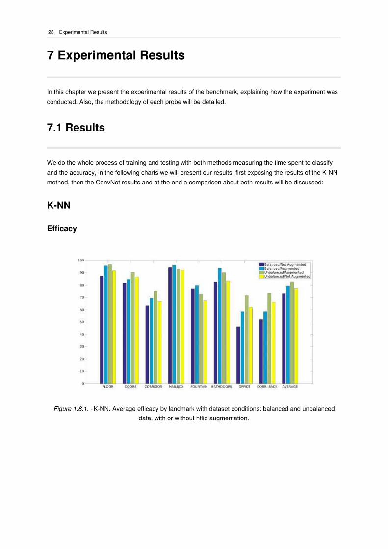
7.1 Results

We do the whole process of training and testing with both methods measuring the time spent to classify

and the accuracy, in the following charts we will present our results, first exposing the results of the K-NN

method, then the ConvNet results and at the end a comparison about both results will be discussed:

K-NN

Efficacy

Figure 1.8.1. - K-NN. Average efficacy by landmark with dataset conditions: balanced and unbalanced

data, with or without hflip augmentation.

28 Experimental Results

L1 L2 L3 L4 L5 L6 L7 L8 AVG MAX

B/NA 87.5 81.73 63.46 94.23 76.92 82.69 46.15 51.92 73.07 94.23

B/A 95.67 84.61 69.23 96.15 79.81 93.75 58.65 58.65 79.56 96.15

U/A 96.65 90.39 75.00 92.93 72.60 90.19 71.50 73.36 82.82 96.65

U/NA 91.75 86.54 66.88 92.25 67.31 83.46 62.12 66.09 77.00 92.25

AVG 92.89 85.81 68.64 93.89 74.15 87.52 59.60 62.50 78.12

MAX 96.65 90.39 75.00 96.15 79.81 93.75 71.50 73.36 82.82

At sight of these results, it can be seen that there are some landmarks more difficult than others : for

example the officce and the corridor back, and both cases work best with balanced and augmented data,

which seems to work better in general. Also, it's worth noting that the other augmented dataset, besides

being unbalanced, scores high too. The fact that both augmented datasets are clearly superior might led

to the following reasoning: either the OpenCV K-NN algorithm implementations fixes the unbalanced

proportions in the trainset or it denotes that the amount of samples radically prevails over the proportions

inside the datasets, furthermore, it contributes to the model's resilience to image alterations.

Time

Figure 1.8.2. - K-NN average time to classify by experiment \(in ms\)

Average time (in ms) to classify

B/NA 0.84

B/A 1.75

U/A 3.46

U/NA 1.79

The chart depicted above shows exactly what we expected: the more samples in the trainset, the more

Experimental Results 29

time spent to classify. This happens due to the way classification works in the K-NN algorithm; when an

item is to be classified it is compared to all the k nearest neighbors, so the higher the amount of near

neighbors, the higher the number of comparisons, hence as the unbalanced, augmented dataset is the

biggest, it also annotates the highest time to classify.

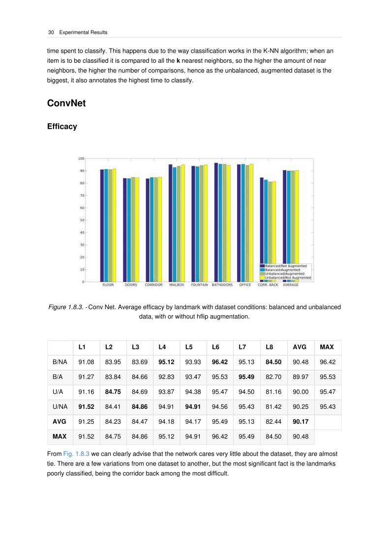
ConvNet

Efficacy

Figure 1.8.3. - Conv Net. Average efficacy by landmark with dataset conditions: balanced and unbalanced

data, with or without hflip augmentation.

L1 L2 L3 L4 L5 L6 L7 L8 AVG MAX

B/NA 91.08 83.95 83.69 95.12 93.93 96.42 95.13 84.50 90.48 96.42

B/A 91.27 83.84 84.66 92.83 93.47 95.53 95.49 82.70 89.97 95.53

U/A 91.16 84.75 84.69 93.87 94.38 95.47 94.50 81.16 90.00 95.47

U/NA 91.52 84.41 84.86 94.91 94.91 94.56 95.43 81.42 90.25 95.43

AVG 91.25 84.23 84.47 94.18 94.17 95.49 95.13 82.44 90.17

MAX 91.52 84.75 84.86 95.12 94.91 96.42 95.49 84.50 90.48

From Fig. 1.8.3 we can clearly advise that the network cares very little about the dataset, they are almost

tie. There are a few variations from one dataset to another, but the most significant fact is the landmarks

poorly classified, being the corridor back among the most difficult.

30 Experimental Results

Time

Figure 1.8.4. - Convolutional Network average time to classify by experiment \(in ms\)

Average time (in ms) to classify

B/NA 161.21

B/A 161.18

U/A 163.71

U/NA 163.12

The convolutional network has a stable classification time, none of the datasets used variate much in the

time spent to classify.

7.2 Comparison

Before comparing the results, a side note must be made: The network and the K-NN classifiers give

different types of outputs, in the case of K-NN, the output is the class of the most representative neighbor,

so it's either correct or incorrect; but in the case of the network, the confidence scores for each label is

given, that means that the output is a range, not a boolean. If we were to compare making a boolean out

of the confidence (ie: keep the highest score), we would have obtained a 100% score on every dataset

and every landmark. As this is not desirable, we took the value of the label with the highest confidence for

the benchmark and average over that scores.

After thoroughly examining the results there are some clear assertions to be made: K-NN outperforms the

network in classify time but looses abruptly when it comes to classify. While K-NN scores, in average,

78.12, the network's final average score is 90.17, that is more than 10 points higher, which in this contexts

means a lot. On the other hand, K-NN classifies almost 200x faster in the best case.

It's worth mentioning that, besides the method used, the corridor back landmark always gets the worst

Experimental Results 31

scores. My best guess is that in the case of K-NN, this happens because of lighting conditions, meaning

that the histogram is not really representative: as can be seen in the dataset, there is a lot of light, the

same principle applies to the office which is basically a window of light. As for the network, I would say this

happens because of the forms inside the picture which in fact, are pretty similar to the corridor, that is

basically the same but in the opposite direction and also scores low.

32 Experimental Results

8 Conclusions and Further Work

At sight of the experimental results it is obvious that both the classic and modern methods can be highly

improved with further study in the lines of preparation of the dataset, parameter initialization and

estimation and data pre-processing, nevertheless the results clearly showed that both methods are a bit

narrow-minded, especially the histogram based K-NN which is easily tricked.

After this experiments we can easily extract a rule of thumb: If time is really crucial (in means of

preparation, training and classification time), go for the K-NN, for everything else go for the Convolutional

Network. Although the process of setting up and training the network is much more intricate and tedious

I'd say it is much more reliable in classification and stable in processing time, which means it can escalate

to a bigger number of classes and dataset sizes with almost constant classification time.

For the K-NN I would like to explore it's limits, as well as it's possible improvements. This algorithm works

surprisingly well, but I feel it could be highly beneficial to use a different metric measure, specially the

Neighborhood Components Analysis [35] which shows very promising results.

As for the ConvNet, I would be delighted to use other setups as the final classification layer, such as

SVMs, a sparsely connected networks or even another little convolutional layer as explained here and

here. The idea is that Fully Connected layers can be really slow, but luckily there is a direct transformation

between the two types without loosing any information, which could only improve the processing time.

Also, it could be great to explore other methods like SVMs, SURF with PCA or Residual Networks and

benchmark them, maybe taking different measures like generalization capabilities or fault-tolerance and

test their comfort boundaries. Taking more classic and modern methods and benchmark them could throw

more light on which methods to choose over the others.

Conclusions and Further Work 33

9 Index of Figures

1By en:User:Cburnett [GFDL (http://www.gnu.org/copyleft/fdl.html]

(http://creativecommons.org/licenses/by-sa/3.0/)))], via Wikimedia Commons.

6A kernel convolution over an image. Taken from [River Trail documentation]

(http://intellabs.github.io/RiverTrail/tutorial/).

5 He, Kaiming et al.. Deep Residual Learning for Image Recognition.

4Yann LeCun et al.. LeNet5, one of the very first successful convolutional networks aimed to digits

recognition.

9 Alex Krizhevsky et al.. AlexNet.

2 Inception v3 - Google Classification Network.

3ConvNet. Average efficacy by landmark with dataset conditions: balanced and unbalanced data,

with or without horizontal flip augmentation. Plotted with matlab.

34 Index of Figures

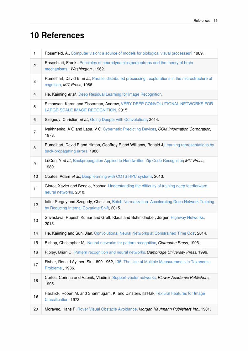
10 References

1 Rosenfeld, A., Computer vision: a source of models for biological visual processes?, 1989.

2Rosenblatt, Frank., Principles of neurodynamics;perceptrons and the theory of brain

mechanisms., Washington,, 1962.

3Rumelhart, David E. et al., Parallel distributed processing : explorations in the microstructure of

cognition, MIT Press, 1986.

4 He, Kaiming et al., Deep Residual Learning for Image Recognition.

5Simonyan, Karen and Zisserman, Andrew, VERY DEEP CONVOLUTIONAL NETWORKS FOR

LARGE-SCALE IMAGE RECOGNITION, 2015.

6 Szegedy, Christian et al., Going Deeper with Convolutions, 2014.

7Ivakhnenko, A G and Lapa, V G, Cybernetic Predicting Devices, CCM Information Corporation,

1973.

8Rumelhart, David E and Hinton, Geoffrey E and Williams, Ronald J, Learning representations by

back-propagating errors, 1986.

9LeCun, Y et al., Backpropagation Applied to Handwritten Zip Code Recognition, MIT Press,

1989.

10 Coates, Adam et al., Deep learning with COTS HPC systems, 2013.

11Glorot, Xavier and Bengio, Yoshua, Understanding the difficulty of training deep feedforward

neural networks, 2010.

12Ioffe, Sergey and Szegedy, Christian, Batch Normalization: Accelerating Deep Network Training

by Reducing Internal Covariate Shift, 2015.

13Srivastava, Rupesh Kumar and Greff, Klaus and Schmidhuber, Jürgen, Highway Networks,

2015.

14 He, Kaiming and Sun, Jian, Convolutional Neural Networks at Constrained Time Cost, 2014.

15 Bishop, Christopher M., Neural networks for pattern recognition, Clarendon Press, 1995.

16 Ripley, Brian D., Pattern recognition and neural networks, Cambridge University Press, 1996.

17Fisher, Ronald Aylmer, Sir, 1890-1962, 138: The Use of Multiple Measurements in Taxonomic

Problems., 1936.

18Cortes, Corinna and Vapnik, Vladimir, Support-vector networks, Kluwer Academic Publishers,

1995.

19Haralick, Robert M. and Shanmugam, K. and Dinstein, Its'Hak, Textural Features for Image

Classification, 1973.

20 Moravec, Hans P, Rover Visual Obstacle Avoidance, Morgan Kaufmann Publishers Inc., 1981.

References 35

21 Harris, Chris and Stephens, Mike, A combined corner and edge detector, 1988.

22 Blake, Andrew and Yuille, A. L. (Alan L.), Active vision, MIT Press, 1992.

23Zhang, Zhengyou et al., A Robust Technique for Matching Two Uncalibrated Images Through

the Recovery of the Unknown Epipolar Geometry, Elsevier, 1995.

24 Dushay, Naomi, Using Structural Metadata to Localize Experience of Digital Content, 2001.

25Yan Ke and Sukthankar, R., PCA-SIFT: a more distinctive representation for local image

descriptors, IEEE, 2004.

26Bay, Herbert and Tuytelaars, Tinne and Van Gool, Luc, SURF: Speeded Up Robust Features,

Springer, Berlin, Heidelberg, 2006.

27 Cover, T. and Hart, P., Nearest neighbor pattern classification, 1967.

28 FISHER, R. A., THE STATISTICAL UTILIZATION OF MULTIPLE MEASUREMENTS, 1938.

29Chapelle, O. and Haffner, P. and Vapnik, V.N., Support vector machines for histogram-based

image classification, 1999.

30 Lecun, Y. et al., Gradient-based learning applied to document recognition, 1998.

31Cirean, Dan Claudiu et al., Deep Big Simple Neural Nets Excel on Hand- written Digit

Recognition, 2010.

32Krizhevsky, Alex and Sutskever, Ilya and Hinton, Geoffrey E, ImageNet Classification with Deep

Convolutional Neural Networks, 2012.

33 Goldberger, Jacob et al., Neighbourhood Components Analysis, 2005.

34Weinberger, Kilian Q and Blitzer, John and Saul, Lawrence K, Distance Metric Learning for

Large Margin Nearest Neighbor Classification, 2005.

35 Goldberger, Jacob et al., Neighbourhood Components Analysis, 2004.

36 References

Appendix 1: Technological Environment

(Software & Hardware)

To program the classic methods we use the well known OpenCV library for Python.

To program the modern, deep neural networks we use transfer learning to Inception v3 with

tensorflow.

Both programs will run in an isolated docker container.

All the work will be developed in a multi-core processor computer (no gpu) with the following specs:

Component Specification

CPU Intel Core i7 - 4790. 4 cores, 3.60GHz, 8MB Smart Cache

RAM 16 GB. DDR 3

Hard Drive SSD 225 GB

SO Arch Linux, kernel 4.4.63-1

Docker 17.04.0-ce, build 4845c567eb

OpenCV OpenCV 3.1.0, Python 2.7

TensorFlow TensorFlow 1.1.0, Python 2.7

Appendix 1: Technological Environment (Software & Hardware) 37

Appendix 2: Resources and Code

Following a brief description of the project's structure and a comprehensible description of each

component:

The project is organized spread across the scripts , src and files directories.

Scripts: Contains all the scripts needed to do the whole preparation: split videos into images,

resize images, augment them, separate datasets into trainset and testset and manage both

docker containers.

Src: This is the source code directory, contains the necessary programs to train and test each

model as well as measure the results and extract the benchmark measures.

Files: Here are contained all the assets for the project: train and test sets of images and dumps

of the data and setup of each model.

The source code directory of each method contains one or various scripts to train and test each model

and in the case of K-NN, the cross validation k − neighbor estimation is provided too.

38 Appendix 2: Resources and Code