Swedish dialect classification using Artificial Neural ...

MASTER’S THESIS

Department of Mathematical Sciences Division of Applied Mathematics and Statistics CHALMERS UNIVERSITY OF TECHNOLOGY UNIVERSITY OF GOTHENBURG Gothenburg, Sweden 2017

Swedish dialect classification using Artificial Neural Networks and Gaussian Mixture Models DAVID LIDBERG VIKTOR BLOMQVIST

Thesis for the Degree of Master of Science

Department of Mathematical Sciences Division of Applied Mathematics and Statistics

Chalmers University of Technology and University of Gothenburg SE – 412 96 Gothenburg, Sweden

Gothenburg, August 2017

Swedish dialect classification using Artificial Neural Networks and Gaussian Mixture Models

David Lidberg Viktor Blomqvist

Swedish Dialect Classification usingArtificial Neural Networks and Gaussian Mixture ModelsDavid LidbergViktor Blomqvist

Copyright c© David Lidberg and Viktor Blomqvist, 2017

Supervisor: Adam Andersson, Syntronic Software InnovationsSupervisor & Examiner: Mihály Kovács, Department of Mathematical Sciences

Master’s Thesis 2017Department of Mathematical SciencesChalmers University of TechnologySE-412 96 GothenburgTelephone +46 31 772 1000

Typeset in LATEXGothenburg, Sweden 2017

ii

Swedish Dialect Classification usingArtificial Neural Networks and Gaussian Mixture ModelsDavid LidbergViktor BlomqvistDepartment of Mathematical SciencesChalmers University of Technology

Abstract

Variations due to speaker dialects are one of the main problems in automatic speechrecognition. A possible solution to this issue is to have a separate classifier identifythe dialect of a speaker and then load an appropriate speech recognition system. Thisthesis investigates classification of seven Swedish dialects based on the SweDia2000database. Classification was done using Gaussian mixture models, which are a widelyused technique in speech processing. Inspired by recent progress in deep learningtechniques for speech recognition, convolutional neural networks and multi-layeredperceptrons were also implemented. Data was preprocessed using both mel-frequencycoefficients, and a novel feature extraction technique using path signatures. Resultsshowed high variance in classification accuracy during cross validations even for simplemodels, suggesting a limitation in the amount of available data for the classificationproblems formulated in this project. The Gaussian mixture models reached thehighest accuracy of 61.3% on test set, based on singe-word classification. Performanceis greatly improved by including multiple words, achieving around 80% classificationaccuracy using 12 words.

Keywords: Swedish, SweDia2000, dialect classification, Gaussian mixture models,convolutional networks, artificial neural networks, deep learning, path signatures.

iii

Acknowledgements

First and foremost we want to express our gratitude to our supervisors AdamAndersson and Mihály Kovács for continued support and feedback throughoutworking with this project. We give thanks to the people behind the Swedia2000project for the data used in this thesis, in particular Anders Eriksson who let us usehis maps for our illustrations. Furthermore we want to thank Syntronic for providingus with the opportunity to work with this project, as well as the department ofMathematical Sciences at Chalmers for letting us use their computational resources.

Viktor Blomqvist and David Lidberg, Gothenburg, June 2017

v

Contents

List of Figures ix

List of Tables xi

1 Introduction 11.1 Delimitations . . . . . . . . . . . . . . . . . . . . . . . . . . . . . . . 21.2 Outline . . . . . . . . . . . . . . . . . . . . . . . . . . . . . . . . . . . 2

2 Dialect Classification 32.1 Speech Corpus . . . . . . . . . . . . . . . . . . . . . . . . . . . . . . . 32.2 Dialect Regions . . . . . . . . . . . . . . . . . . . . . . . . . . . . . . 52.3 Classification . . . . . . . . . . . . . . . . . . . . . . . . . . . . . . . 5

2.3.1 Wordwise . . . . . . . . . . . . . . . . . . . . . . . . . . . . . 72.3.2 Generalization to Spontaneous Speech . . . . . . . . . . . . . 7

3 Signature Theory 93.1 Preliminaries . . . . . . . . . . . . . . . . . . . . . . . . . . . . . . . 9

3.1.1 Tensor Product Spaces . . . . . . . . . . . . . . . . . . . . . . 93.1.2 Formal Power Series . . . . . . . . . . . . . . . . . . . . . . . 103.1.3 Paths and Line Integrals . . . . . . . . . . . . . . . . . . . . . 13

3.2 Signature Definition . . . . . . . . . . . . . . . . . . . . . . . . . . . 143.3 Log Signature . . . . . . . . . . . . . . . . . . . . . . . . . . . . . . . 153.4 Practical Calculations . . . . . . . . . . . . . . . . . . . . . . . . . . 17

3.4.1 Chen’s Identity . . . . . . . . . . . . . . . . . . . . . . . . . . 183.4.2 Recursive Iterated Integral Expressions . . . . . . . . . . . . . 203.4.3 Log Signatures . . . . . . . . . . . . . . . . . . . . . . . . . . 24

4 Feature Extraction 254.1 Short-Time Fourier Transform . . . . . . . . . . . . . . . . . . . . . . 254.2 Mel-Frequency Spectral Coefficients . . . . . . . . . . . . . . . . . . . 264.3 Mel-Frequency Cepstral Coefficients . . . . . . . . . . . . . . . . . . . 28

4.3.1 Shifted Delta Cepstra . . . . . . . . . . . . . . . . . . . . . . . 294.4 Log Signatures as Acoustic Features . . . . . . . . . . . . . . . . . . . 304.5 Normalization . . . . . . . . . . . . . . . . . . . . . . . . . . . . . . . 31

5 Classifiers 335.1 Gaussian Mixture Models . . . . . . . . . . . . . . . . . . . . . . . . 33

5.1.1 Training . . . . . . . . . . . . . . . . . . . . . . . . . . . . . . 345.1.2 Classification . . . . . . . . . . . . . . . . . . . . . . . . . . . 36

vii

Contents

5.2 Artificial Neural Networks . . . . . . . . . . . . . . . . . . . . . . . . 365.2.1 Network Building Blocks . . . . . . . . . . . . . . . . . . . . . 375.2.2 Network Architectures . . . . . . . . . . . . . . . . . . . . . . 405.2.3 Training . . . . . . . . . . . . . . . . . . . . . . . . . . . . . . 42

6 Experiments 456.1 Generalization . . . . . . . . . . . . . . . . . . . . . . . . . . . . . . . 45

6.1.1 K-Fold Cross-Validation . . . . . . . . . . . . . . . . . . . . . 466.2 Metrics . . . . . . . . . . . . . . . . . . . . . . . . . . . . . . . . . . . 46

6.2.1 Confusion Matrix . . . . . . . . . . . . . . . . . . . . . . . . . 476.3 Single-word Calibration . . . . . . . . . . . . . . . . . . . . . . . . . . 476.4 Multi-word Classification . . . . . . . . . . . . . . . . . . . . . . . . . 48

6.4.1 Splitting . . . . . . . . . . . . . . . . . . . . . . . . . . . . . . 486.4.2 Forward Selection . . . . . . . . . . . . . . . . . . . . . . . . . 49

6.5 Spontaneous Speech Classification . . . . . . . . . . . . . . . . . . . . 49

7 Results 517.1 Hyperparameter Calibration . . . . . . . . . . . . . . . . . . . . . . . 51

7.1.1 Gaussian Mixture Models . . . . . . . . . . . . . . . . . . . . 517.1.2 Multilayer Perceptron . . . . . . . . . . . . . . . . . . . . . . 517.1.3 Convolutional Neural Network . . . . . . . . . . . . . . . . . . 527.1.4 Modular Network . . . . . . . . . . . . . . . . . . . . . . . . . 53

7.2 Performance on Calibration Words . . . . . . . . . . . . . . . . . . . 537.3 Multi-word Performance . . . . . . . . . . . . . . . . . . . . . . . . . 547.4 Other Signature-based Implementations . . . . . . . . . . . . . . . . . 577.5 Spontaneous Speech Classification . . . . . . . . . . . . . . . . . . . . 577.6 Effect of Speaker Identity . . . . . . . . . . . . . . . . . . . . . . . . 58

8 Conclusions 61

A Tables 63

Bibliography 68

viii

List of Figures

2.1 SweDia2000 recording locations. From [1]. Reproduced with permis-sion from the copyright holder. . . . . . . . . . . . . . . . . . . . . . 4

2.2 A map showing the division of SweDia recording locations into sevensub-regions, used as dialects. From [1]. Adapted with permission fromthe copyright holder. . . . . . . . . . . . . . . . . . . . . . . . . . . . 6

4.1 Fourier spectrogram. The figure shows logarithm of the pixel valuesfor illustrativ purposes. . . . . . . . . . . . . . . . . . . . . . . . . . 26

4.2 Mel-scale filter bank with 15 filters. . . . . . . . . . . . . . . . . . . . 274.3 Mel spectrogram of the word dagar from a dalarna dialect . . . . . . 284.4 Spectrogram that has been decorrelated using a discrete cosine trans-

form, hence a cepstrogram. The columns in the figure are MFCCfeature vectors. Commonly only coefficients 0-12 are used, whichmeans the other rows in the figure are discarded. . . . . . . . . . . . 29

5.1 An example of how the distribution of cluster of data points in R2 canbe approximated with a GMM constructed with the EM algorithm. . 35

5.2 Artificial neural network with four-dimensional input and two hiddenlayers, mapping to two output nodes. The arrows between the neuronsshow the structure of the connections. . . . . . . . . . . . . . . . . . . 40

5.3 Example of a convolutional neural network architecture with twoconvolutional layers with max-pooling layers between them. The finaltwo layers of the network are fully connected layers. . . . . . . . . . . 41

5.4 Modular network setup for a case when two different types of inputare available. Module A and B process different inputs, and theiroutputs are concatenated and fed to a decision module that performsclassification. . . . . . . . . . . . . . . . . . . . . . . . . . . . . . . . 42

7.1 Normalized confusion matrix for a Gaussian mixture model on theword kaka. . . . . . . . . . . . . . . . . . . . . . . . . . . . . . . . . . 54

7.2 Normalized confusion matrix for a convolutional neural network onthe word kaka. . . . . . . . . . . . . . . . . . . . . . . . . . . . . . . . 55

7.3 Average validation set accuracy over three independent training runsfor ensemble classifiers combining multiple single-word classifiers viaforward selection. . . . . . . . . . . . . . . . . . . . . . . . . . . . . . 56

7.4 Normalized confusion matrix for a multi-word GMM using a forwardselected set of words. . . . . . . . . . . . . . . . . . . . . . . . . . . . 57

ix

List of Figures

7.5 Four word utterances. The two upper figures are from the samespeaker uttering the word jaga. The bottom left is also from thisspeaker, uttering saker. Bottom right is again jaga but from a differentspeaker. . . . . . . . . . . . . . . . . . . . . . . . . . . . . . . . . . . 59

A.1 Normalized confusion matrix for the Gaussian mixture model on theword kaka. . . . . . . . . . . . . . . . . . . . . . . . . . . . . . . . . . 64

A.2 Normalized confusion matrix for the Convolutional network on theword kaka. . . . . . . . . . . . . . . . . . . . . . . . . . . . . . . . . . 64

A.3 Normalized confusion matrix for a multi-word GMM using a forwardselected set of words. . . . . . . . . . . . . . . . . . . . . . . . . . . . 65

x

List of Tables

2.1 The SweDia2000 recording locations assigned to each dialect region. . 62.2 Percentage of audio files which have a corresponding annotation file

per dialect region. . . . . . . . . . . . . . . . . . . . . . . . . . . . . . 7

3.1 Word splitting of w = (i, j, k) as a result of g2(w). The operatorgathers all words u1 and u2 so that u1u2 = w. . . . . . . . . . . . . . 19

3.2 An example of how the operator s(·) works, here applied on the word(1, 2, 3, 4), i.e. (u, v) ∈ s(1, 2, 3, 4). . . . . . . . . . . . . . . . . . . . . 20

7.1 Tested hyperparameters when calibrating the Gaussian Mixture Modelclassifier for single word dialect classification. . . . . . . . . . . . . . . 52

7.2 Average test set classification accuracy over 5-fold cross-validation onthe four calibration words for hyperparameter-calibrated classifiers. . 53

7.3 Average classification accuracy and number of words selected overthree random initializations of multiword data. . . . . . . . . . . . . 56

A.1 The number of unique speakers in each dialect region as well asinformation about how many speakers in each dialect provides at leastn utterances for every wordlist word. . . . . . . . . . . . . . . . . . . 65

A.2 Number of utterance available per word in each dialect in the wordlistcategory. Only words occurring frequently across all seven dialectsare included. . . . . . . . . . . . . . . . . . . . . . . . . . . . . . . . . 66

A.3 Average ranking of words in forward selection, sorted from best toworst overall ranking. Blue rows indicate words used for calibration. . 67

xi

Chapter 1

Introduction

There are several factors that affect human speech. There are speaker-to-speakervariations — humans can often identify a person from their voice based solely on afew words. Age, gender and emotional state are other factors that have an impacton speech [2]. One of the challenges in automatic speech recognition (ASR) is toovercome such sources of variation. This thesis focuses on a particular factor, namelythe dialects of speakers. Dialects can come with different pronunciations of wordsand phones, tone of voice and even completely different words, and can thereforehave significant impact on performance of speech recognition systems [3]. Dialectclassification is an approach to address this difficulty. By first determining the dialectof a speaker, an ASR system adapted for that dialect can be activated and thusimprove recognition accuracy.

Previous research on dialect classification have taken various approaches. Classifi-cation of American accents based acoustic features of specific words were investigatedin [4]. Phonetic context has been used to classify Arabian dialects, where the dialectsare identified based the order of phonemes [5]. Both these works are based on Mel cep-stral features, which are standard features in many speech processing applications [6].More linguistical approaches involve vocabularies and lexical features [7].

This thesis investigates Swedish dialect classification, and compares methods forachieving such a classification. The study covers Gaussian mixture models (GMMs),which is a standard technique in ASR and has been used for dialect classification aswell [8–10]. In fact, ASR and dialect classification, as well as speaker and genderidentification, are generally implemented using similar methods. While GMMshistorically have been successful in ASR applications, recently deep artificial neuralnetworks have risen as a strong candidate to replace GMM’s [11, 12]. Thereforethis thesis also investigates the performance of a convolutional neural network andmulti-layered perceptrons in dialect classification.

In addition to the standard features centered around the Mel scale new methodsinvolving the signature transform is tested as feature extraction. The signature is anon-linear transformation with roots in rough paths theory [13]. By calculating thesignature of a path one obtains a collection of coefficients that contains propertiesof that path. Signatures and the closely related log signatures have recently beensuccessfully implemented in Chinese character recognition [14] and studied as amethod for sound compression [15]. Whilst the project does not aim to extendthe theory behind signatures, deriving and implementing efficient procedures forcalculating the transform is a part of the project outcome.

1

Chapter 1. Introduction

Implementation are written in Python 3 with the exception of a shared librarywritten in C. Scikit-learn1 and Tensorflow2 are the main libraries used for classifiers.

1.1 Delimitations

This thesis focuses solely on acoustic speech features, relating more or less directlyto the original sound signal. This is partly motivated by the fact that prosodical andsimilar features are linguistically complex and require thoroughly annotated soundsamples.

Furthermore the main part of classification experiments deal with dialect clas-sification based on utterances of single words, or multiple utterances of differentwords. This is in contrast to spontaneous speech which is perhaps the more commonvariant of raw data. The incorporation of dialect identification into automatic speechrecognition, possibly improving performance, is not tested.

As no examples of Swedish dialect classification with defined dialect regions havebeen found, seven dialects are presented and used here for the first time.

1.2 Outline

Chapter 2 introduces the data which is later used for experiments, defines dialectsand outlines the type of experiments that are possible given the data and dialects.In Chapter 3 the theory behind signatures and log signatures of paths is introducedalong with the necessary preliminaries. Expressions for calculating these in practiceunder some assumptions are also presented.

Thereafter the focus changes to machine learning with Chapter 4 that introducestypical feature extraction methods for speech data and Chapter 5 in which theclassifiers used in the thesis are explained. Chapter 6 explains the details of theexperiments and the results of these together with comments are presented in Chapter7. Lastly, Chapter 8 contains conclusions and reflections on the work.

1http://scikit-learn.org2https://www.tensorflow.org/

2

http://scikit-learn.org

https://www.tensorflow.org/

Chapter 2

Dialect Classification

Dialect classification, also called dialect identification, is the problem of detectingand classifying different ways of speaking the same language. A strict interpretationof dialect would be versions of a language with different phrases or words, and accentthen meaning variants of pronunciation. In this thesis we use dialect to indicatevariance in both word choices and pronounciation.

2.1 Speech Corpus

The data used in this thesis comes from SweDia 20001, a research database containingSwedish speech recordings [16]. The data consists of interviews with people at overone hundred different locations in Sweden and Swedish-speaking parts of Finland,as shown in Figure 2.1. At each location there are interviews from, on average, 12different persons residing in the local area. The interviewed persons are all adultbut divided by age and gender. Generally 3 elderly males, 3 elderly females, 3 youngmales and 3 young females at each location. The average age of in these demographicgroups are, 66, 66, 26 and 25 years old respectively.

The database is further divided into four different categories, each one correspond-ing to a type of interview. The four categories are quantity, prosody, wordlist andspontaneous. The first three extract multiple utterances of predefined words. Thespecific words depends on the category and in some cases the recording location. Outof these three categories, only wordlist is used since its content varies less betweendifferent recording locations and contains a larger number of words. In contrast tothe other three, the spontaneous interviews do not follow a script. As the namesuggests each interview is actually a spontaneous dialogue between an interviewerand one (sometimes two) interviewee(s).

Most audio files in the database are accompanied by an annotation file containinga transcription of what is said and by whom. These files make it possible todivide audio from the interviewer and interviewee. This is necessary since only theinterviewee can be assumed to have a dialect tied to the location where the recordingtook place. Since transcribing speech is very time consuming not all audio-files in thedatabase have been annotated. The coverage is especially sparse in the spontaneouscategory, where transcription is very time consuming.

The sound files are in the Waveform Audio File Format (commonly referred to

1http://swedat.ling.gu.se/

3

http://swedat.ling.gu.se/

Chapter 2. Dialect Classification

Recordings• 107 locations

– 31 Northern parts of Sweden 3 Ostrobothnia (Finland)

– 27 Central parts of Sweden 7 Nyland och Åland

– 39 Southern parts of Sweden• 12 speakers per location

– 3 older men 51–89, M 66– 3 older women 42–84, M 66– 3 younger men 19–40, M 26– 3 younger women 17–36, M 25

• In totalt about 1300 speakers

SweDia2000

AsbyJärsnäs

RimforsaKorsberga

Stenberga

Ankarsrum

Burseryd

Floby

Frillesås

ÖxabäckKärna

Orust S:t Anna

Böda Sproge

Fole

Segerstad

Väckelsång

Torsås

Bredsätra

Jämshög

Torhamn

Hamneda

Broby

Hällevik

Össjö

N. Rörum

TjällmoV. Vingåker

Viby LännaSt. Mellösa

Sorunda

Haraker

SkinnskattebergVillberga

Skuttunge

JärnboåsGåsborn

GräsmarkGrangärdeMalung

Kårsta

Nora

ÅrsundaGräsö

OckelboLeksand

Orsa SkogOvanåker

Saltvik

Dalby

Älvdalen

Brändö

Fårö

Skee

Köla

Skillingmark

S, Finnskoga

Årstad-Heberg

Våxtorp

DelsboFärilaLillhärdal

Bjuv

Närpes

VöråKramforsRagunda

Piteå

Bjurholm

Houtskär

Dragsfjärd

Särna

Munsala

Snappertuna

Kyrkslätt

Strömsund Fjällsjö

LöderupBara

Nysätra

Borgå

Anundsjö

Arjeplog

Aspås

Bengtsfors

Berg

BurträskFrostviken

Frändefors

Indal

KalixNederluleå

Sorsele

Storsjö

Torp

Torsö

Vemdalen

Vilhelmina

Vindeln

Åre

Östad

Överkalix

Figure 2.1: SweDia2000 recording locations. From [1]. Reproduced with permission fromthe copyright holder.

4


as wav) recorded as mono sound (with a few exceptions). The bit depth is 16 bitsand sample rate 16kHz.

2.2 Dialect Regions

Clearly defined dialects is a precondition for performing dialect classification. Onecould argue that every recording location represents its own (albeit very local) dialect.Such micro-dialects are however unfeasible in practice as there would not be enoughdata available in each dialect.

It is therefore necessary to pool together recording locations in close geographicalproximity into larger dialect regions. One such division of the Swedish language areawas proposed by Wessén in [17] which divided the area into six regions of varyingsize. However, pooling into too large regions leads to ambiguity in where to drawthe borders between dialects, as there are no clear cut lines between dialects [17].

To get around these problems we define a set of seven dialect regions, partlyinspired by Wesséns division. Out of Wesséns six regions, only Gotland is too small,and it is therefore dropped from our definition. Furthermore we have chosen tosplit the northern part of Sweden in two, as it is geographically the largest. Thisalso provides an opportunity for studying the variance inside what is a single regionaccording to Wessén. We also include the Swedish province Dalarna, located inthe central west part of mainland Sweden, as its own dialect region, since it is adistinct and recognizable dialect [18]. This leaves us with the seven dialects/regions:Norrbotten, Jämtland, Dalarna, Sydfinland, Mälardalen, Västkusten and Skåne.

Finally, all regions are not included in full, rather locations from internal subsetsof some regions are chosen to represent the dialect, providing a margin betweendialect areas and regions of comparable size. In column two of Table A.1 we see thatthe numbers of unique speakers in each dialect are relatively balanced.

Our seven dialect regions are shown in Figure 2.2. The exact locations included ineach dialect is presented in Table 2.1. The discrepancy between the figure and tablespecifying dialect regions is due to unusable locations in the database. The locationsÄlvdalen and Orsa, inside the Dalarna region, and Bjuv in Skåne are marked on themap but contain none or very few files in the version of the database we used, andwere dropped from the corresponding regions. To compensate for this, Dalarna andSkåne were expanded to balance the number of speakers across dialects, meaningthey look larger on the map but they are in fact not larger in data size.

2.3 Classification

As mentioned above, only data from the wordlist and spontaneous categories areused in this thesis. The annotation coverage in each of the categories across theseven dialects is presented in Table 2.2. Clearly, annotations are not a problem inthe wordlist category. The situation is as expected less optimistic in spontaneous.Based on these data limitations, two different experimental approaches to dialectclassification are formulated below.

5


Norrbotten

Jämtland

Skåne

SydfinlandDalarna

Västkusten

Mälardalen

Figure 2.2: A map showing the division of SweDia recording locations into seven sub-regions, used as dialects. From [1]. Adapted with permission from the copyright holder.

Table 2.1: The SweDia2000 recording locations assigned to each dialect region.

Norrbotten Jämtland Sydfinland Dalarna Mälardalen Västkusten Skåne

Arjeplog Åre Borga SödraFinnskoga Skuttunge Orust Vaxtorp

Överkalix Aspås Kyrkslätt Dalby Villberga Frändefors Broby

Nederkalix Frostviken Snappertuna Malung Haraker Kärna Össjö

Piteå Berg Dragsfjärd Leksand Kårsta Östad Bara

Sorsele Strömsund Houtskär Grangärde Länna Öxabäck Löderup

Nederluleå Ragunda Brändö Husby Sorunda Frillesås NorraRörum

Sarna Graso

6


Table 2.2: Percentage of audio files which have a corresponding annotation file per dialectregion.

Dialect Spontaneous (%) Wordlist (%)

Norrbotten 21.13 100.00Jämtland 34.92 100.00

Sydfinland 29.17 97.22Dalarna 6.58 98.86

Mälardalen 19.72 100.00Västkusten 10.96 100.00

Skåne 37.50 100.00

Overall 22.49 99.45

2.3.1 Wordwise

Our first experiment category ignores the spontaneous data completely and focuseson utterances of single words from the wordlist category of interviews. With dialectsdefined, the frequency of words in the data can be studied. Out of all the differentwords uttered in wordlist interviews, 43 words occur frequently across all dialects,shown in Table A.2.

Four of the most frequently occurring: dörr, flytta, kaka and lär, are selectedas calibration words. This is necessary since classifiers are set up and tuned basedon data, but calibrating each classifier for each of the 43 words would be too timeconsuming. By limiting calibration to four words we hope to find hyperparameterswhich are suitable for capturing the complexity in single-word dialect classifications.It is assumed that a classifier setup which works well for the four calibration wordswill generalize without great loss of performance to the other 39 words.

It is then possible to evaluate the performance of dialect classifiers which operateon utterances of one specific word, and also find which words among the 43 are bestsuited for dialect classification. Lastly it is tested if combining multiple single-wordclassifiers into an ensemble classifier which takes a tuple of word utterances from asingle speaker as input can be used to further improve performance.

2.3.2 Generalization to Spontaneous Speech

Compared to word-specific dialect classifiers, classifying spontaneous speech is ar-guably more practical, mostly due to the fact that a spontaneous classifier does notrequired predefined to perform classification.

The limited annotation coverage in the spontaneous category prohibits bothtraining and evaluating classifiers on spontaneous speech. Instead we test if aclassifier trained on the complete set of wordlist single word utterances (all 43 words),performs well when evaluated on spontaneous data. This tests if utterances of singlewords contain the same, or similar, dialectal markers as spontaneous speech.

7

Chapter 3

Signature Theory

In this chapter we introduce the concept of expressing information about a path inRd by its signature. Formal power series and iterated integrals are introduced asthese are necessary when defining the signature. We also present explicit expressionsfor transforming the signature into a log signature, and derive methods for practicalsignature and log signature calculations.

3.1 Preliminaries

This section provides a short overview of the mathematics used later in this chapter.

3.1.1 Tensor Product Spaces

The tensor product of two inner product spaces U and V is the space U ⊗ V , herecalled W . If there is a bilinear map ⊗ so that

U × V → W, (u, v) 7→ u⊗ v

and W has an inner product 〈·, ·〉W so that for u1, u2 ∈ U and v1, v2 ∈ V

〈u1 ⊗ v1, u2 ⊗ v2〉W = 〈u1, u2〉U〈v1, v2〉V (3.1)

holds, we will callW the tensor product space corresponding to a particular ⊗, whichin this thesis will always be the outer product.

If the spaces U and V are spanned by basis vectors eu1 , . . . , eum and ev1, . . . , e

vn,

then W is the space spanned by the basis of paired vectors eui ⊗ evj for (i, j) ∈{1, . . . ,m} × {1, . . . , n}. Hence we have for the dimension of W that

dim(W ) = dim(U)dim(V ).

Another consequence of this is that any element w ∈ W can be be written as

w =

m,n∑i,j=1

wi,j(eui ⊗ evj ).

It follows that for elements u ∈ U and v ∈ V on the form

u =m∑i=1

uieui and v =

n∑j=1

vjevj

9

Chapter 3. Signature Theory

we can construct the object u⊗ v ∈ W as

u⊗ v =

m,n∑i,j=1

uivj(eui ⊗ evj ).

For an n-fold tensor product of an element v ∈ V , we use the notation

v⊗n = v ⊗ v ⊗ · · · ⊗ v︸︷︷︸n

.

The object v⊗n is an element of V ⊗n which is defined analogously.We can also join spaces U and V with direct summation, constructing a new

space W = U ⊕ V . The direct summation is similar to the Cartesian product, inthat the resulting space W consists of all possible ordered pairs of elements from Uand V . The direct summation however, also defines addition on W . With u1, u2 ∈ Uand v1, v2 ∈ V the addition on W is defined as

(u1, v1) + (u2, v2) = (u1 + u2, v1 + v2).

The basis of W will be the combined set of basis elements from U and V , withslight modification. Using the notation (ei, 0) or (0, ej) to indicate basis vectorspaired with a zero vector (from V or U respectively) together with standard notationfor basis vectors in U and V , the set of vectors (eu1 , 0), . . . , (eum, 0), (0, ev1), . . . , (0, e

vn)

make up a basis for W . From this we can see that dim(W ) = dim(U) + dim(V ).

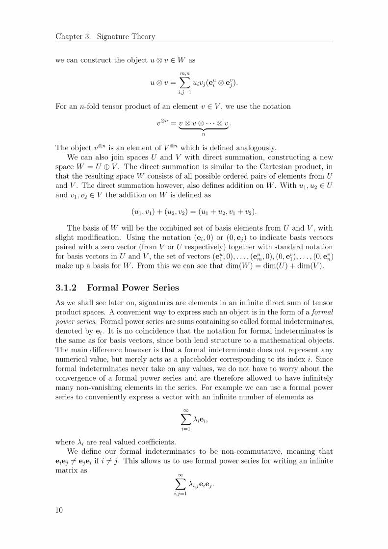
3.1.2 Formal Power Series

As we shall see later on, signatures are elements in an infinite direct sum of tensorproduct spaces. A convenient way to express such an object is in the form of a formalpower series. Formal power series are sums containing so called formal indeterminates,denoted by ei. It is no coincidence that the notation for formal indeterminates isthe same as for basis vectors, since both lend structure to a mathematical objects.The main difference however is that a formal indeterminate does not represent anynumerical value, but merely acts as a placeholder corresponding to its index i. Sinceformal indeterminates never take on any values, we do not have to worry about theconvergence of a formal power series and are therefore allowed to have infinitelymany non-vanishing elements in the series. For example we can use a formal powerseries to conveniently express a vector with an infinite number of elements as

∞∑i=1

λiei,

where λi are real valued coefficients.We define our formal indeterminates to be non-commutative, meaning that

eiej 6= ejei if i 6= j. This allows us to use formal power series for writing an infinitematrix as

∞∑i,j=1

λi,jeiej.

10


With formal power series, we can represent tensors of arbitrary order. A series ofone index of indeterminates constitutes a first order tensor, or vector. Two indicesallows us to represent matrices, as above, and three indices would represent a third-order tensor, etc. Since the addition of two formal power series is practically directsummation, we can write a mathematical object which is a vector and a matrix as

∞∑i=1

λiei +∞∑

i,j=1

λi,jeiej.

We will use addition for formal power series to represent both direct summation andstandard addition. Should two formal indeterminates be identical during addition oftwo formal power series, standard component-wise addition is done. For differingindeterminates, addition refers to direct summation and extends the dimensionalityof the object.

To represent constants in formal power series, we define the special emptyindeterminate e∅ which is implicitly placed after all terms that do not already haveindeterminates. This indeterminate is special in that e∅ei = ei, which means alloperations we want to use also hold when scalars are present.

Another operation which we let formal power series inherit from the tensorproduct spaces is the inner product, but only between formal power series withfinitely many terms, as else problems with convergence would arise. For example,the inner product between two vectors F and G with d elements, represented by thefinite formal power series

F =d∑i=1

λ(F )i ei and G =

d∑i=1

λ(G)i ei,

is

〈F,G〉 =d∑i=1

λ(F )i λ

(G)i .

The inner product also extends naturally to object constructed from the directsummation and tensor products. For example, for F and G such as

F =d∑i=1

λ(F )i ei +

d∑i,j=1

λ(F )i,j eiej,

G =d∑i=1

λ(G)i ei +

d∑i,j=1

λ(G)i,j eiej

we have:

〈F,G〉 =d∑i=1

λ(F )i λ

(G)i +

d∑i,j=1

λ(F )i,j λ

(G)i,j .

The inner product can also be used even when there isn’t a perfect symmetrybetween the formal indeterminates in both arguments. We can practically view everyformal power series as containing every possible indeterminate combination, but with

11


coefficient 0 for the ones we don’t see. An example of this would be two vectors withdifferent lengths, written as

F =

dF∑i=1

λ(F )i ei and G =

dG∑i=1

λ(G)i ei

where dF < dG. The inner product between these vectors is then

〈F,G〉 =

dF∑i=1

λ(F )i λ

(G)i .

Lastly, we want to point that we can construct arbitrary tensors, i.e elements ofthe tensor product spaces, with formal power series. For example the two formalpower series

F =d∑

i1=1

. . .d∑

ik=1

λ(F )i1,...,ik

e1 . . . ek and G =d∑

i1=1

. . .d∑

ik=1

λ(G)i1,...,ik

e1 . . . ek,

are kth order tensors with d dimensions. The inner product between these two formalpower series, defined in (3.1), is the sum

〈F,G〉 =d∑

i1=1

. . .d∑

ik=1

λ(F )i1,...,ik

λ(G)i1,...,ik

.

This shows us that formal power series are related to inner product spaces.Therefore we want to introduce the tensor product operation to the formal power seriesnotation. First of all we define the tensor product between two formal indeterminatesei and ej to be ei ⊗ ej = eiej, satisfying (aei)⊗ (bej) = abeiej for any a, b ∈ R andhaving the distributive property (ei+ej)⊗ (ek +e`) = eiek +eie`+ejek +eje`. Thisdistributive property means that a tensor product is also defined between formalpower series, since these are simply sums of indeterminate terms.

For finite formal power series, this definition exactly mimics, by design, the tensorproduct related to inner product spaces presented in Section 3.1.1. This is the reasonfor having non-commutative formal indeterminates with the same behaviour as theouter product that we use as bilinear map. The tensor product for two finite formalpower series F and G is then by definition

F ⊗G =d∑i=1

λ(F )i ei ⊗

d∑j=1

λ(G)j ej =

d∑i,j=1

λ(F )i λ

(G)j eiej.

For infinite formal power series the behaviour of the tensor product is very similarto the finite case. For example the tensor product between the two infinite formalpower series

F =∞∑i=1

λ(F )i ei and G =

∞∑j=1

λ(G)j ej

12


is by definition

F ⊗G =∞∑i=1

λ(F )i ei ⊗

∞∑j=1

λ(G)j ej =

∞∑i,j=1

λ(F )i λ

(G)j eiej.

For infinite formal power series, however, the tensor product must differ fromthat of Section 3.1.1, since such series are, as noted above, not equipped with aninner product. This means that the tensor product between formal power series is ageneralization, accommodating both finite and infinite series.

We will also preserve the notation of n-times repeated tensor products as F⊗nfor formal power series.

3.1.3 Paths and Line Integrals

A path is a continuous function X : [a, b]→ Rd which intuitively can be understoodas a point moving through the space Rd over the time interval [a, b]. A path is said tobe smooth if the first derivative X : [a, b]→ R exists and is continuous on [a, b]. Theintegral of an integrable function f : Rd → R over a smooth path X : [a, b]→ Rd isdefined as

b∫a

f(Xt) dXt =

b∫a

f(Xt)Xt dt.

If X is not smooth on the whole of [a, b] but rather piecewise smooth on thepartitions a = t0 < t1 < . . . < tn = b the line integral over X is defined as the sumof path integrals over each smooth segment

b∫a

f(Xt) dXt =

t1∫t0

f(Xt) dXt +

t2∫t1

f(Xt) dXt + . . .+

tn∫tn−1

f(Xt) dXt.

As X = (X1, . . . , Xd) each X i, which describes the change of X in direction i,is itself a path, but in R instead of Rd. The line integral of the constant functionf = 1 over one of the coordinate paths X i in an interval with an endpoint decidedby t ∈ [a, b] is

I(X)(i)a,t =

t∫a

1 dX is =

t∫a

X is ds = X i

t −X ia

which, again, is a path in R. Since it is possible to integrate functions mapping Rinto itself over paths in R we can integrate I(X)

(i)a,t along any of the paths describing

the change of X. If Xj is one of these paths, the function

I(X)(i,j)a,t =

t∫a

I(X)(i)a,s dXjs =

t∫a

s∫a

dX ir dXj

s =

t∫a

s∫a

X ir drXj

s ds

is yet another path in R. This wrapping of the single dimensional paths describingthe change of X leads to the concept of iterated integrals. The real number I(X)

(i)a,b

13


is the 1-fold iterated integral of X along index i. The 2-fold iterated integral wouldbe I(X)

(i,j)a,b which is along the pair of indices i, j. The general formula for a k-fold

iterated integral is made over a sequence of k indices i1, . . . , ik and is the real number

I(X)(i1,...,ik)a,b =

∫a<tk<b

I(X)(i1,...,ik−1)a,tk

dX iktk

=

∫a<tk<b

. . .

∫a<t1<t2

dX i1t1 . . . dX

iktk.

3.2 Signature Definition

The signature of a path is closely related to iterated integrals, in fact it is the infinitecollection of all iterated integrals along the path. A collection of real numbers whichcontains information about the path [19]. By using formal power series we canexpress this infinite set of numbers in a structured manner.

First we generalize the series of indices used in iterated integrals by introducinga lexical notation. Given a path X = (X1, X2, . . . , Xd) we call each index i a letterbelonging to the alphabet A = {1, 2, . . . , d}. Finite sequences of indices are calledwords and, if of finite length, are written as w = (i1, i2, . . . , ik) with |w| denotingthe number of letters in w so that |w| = k. For a given alphabet there is an infinitenumber of possible words if no limit on word length is imposed. This set of wordsis denoted by W and contains the special empty word ∅ which has no letters and|∅| = 0. With this notation we write iterated integrals as I(X)wa,b where each letterij in w represents an integral along X ij . The iterated integral with respect to theempty word is equal to one by definition.

The signature of a path X is the collection of all iterated integrals correspondingto words in the infinite set W . To write this mathematical object in a meaningfulway we will use formal indeterminates as placeholders for letters.

Definition 1. The signature of a path X : [a, b]→ Rd is the formal power series

S(X)a,b =∞∑k=0

∑i1,...,ik∈A

I(X)(i1,...,ik)a,b ei1ei2 . . . eik .

The outer summation is over the length k of words, also called the level of thesignature. The zeroth level contains only a single element which is equal to 1 bydefinition. The first level holds all iterated integrals based on one-letter words, andso for a d-dimensional path, the first level resides in Rd. The second level is a matrixin Rd ⊗ Rd, and the third is a tensor in (Rd)⊗3. This increase in the dimension ofthe space which each signature level resides in continues indefinitely. The entiresignature resides in a space given by direct summation of each level-space, hence asignature is an element in T (Rd) =

⊕∞k=0(Rd)⊗k.

Expressed as this formal power series, the operations defined in Section 3.1.2can be applied to or between signatures1. An important result in the theory ofsignatures is that the tensor product of two signatures (corresponding to paths ofequal dimensionality) will also be in T (Rd) and is therefore a valid signature. This isdue to, and the reason behind, the zeroth level being defined as 1.

1Since signatures are infinite formal power series, this refers to the tensor product without aninner product.

14


3.3 Log Signature

While the signature is a full representation of its path, not all of its elements areindependent. The log signature is a condensed representation, and contains the sameinformation expressed with significantly fewer and independent elements [15].

This section demonstrates a method for extracting a basis representation for thelog signatures, and we use the short-hand notation λw = I(X)wa,b to make calculationsmore readable. We begin by writing the signature as the formal power series

S(X)a,b = 1 +∞∑k=1

∑i1,...,ik∈A

λ(i1,...,ik)ei1ei2 . . . eik

with the term corresponding to the empty word moved out of the sum. The logarithmof a formal power series F = a0 +

∑∞k=1 akek is defined as

logF = log a0 +∞∑n=1

(−1)n

n

(1− F

a0

)⊗n.

Combining this definition with the signature gives

logS(X) =∞∑n=1

(−1)n+1

n

∞∑k=1

∑i1,...,ik∈A

λ(i1,...,ik)ei1ei2 . . . eik

⊗n (3.2)

which has terms corresponding to every word in W except the empty word. Wedefine W ∗ to be the set of all non-empty words, and let ew denote the basis elementfor each letter in w, i.e. ew = ei1 . . . eik if w = (i1, . . . , ik). Using this notation wewant to find a number λw for every w ∈ W ∗ so that (3.2) can be rewritten as

logS(X) =∑w∈W ∗

λwew. (3.3)

For an arbitrary word w of length |w| > 0, all contributions to λw comes fromthe first |w| tensor products in (3.2). Any higher n will only give rise to words longerthan w. Let the concatenation of two words u = (u1, . . . , uk) and v = (v1, . . . , v`) bewritten as uv = (u1, . . . , uk, v1, . . . , v`). Then we can use w1 . . . wn = w to indicate asummation over all possible ways of splitting w into n non-empty subwords. Thesought coefficient corresponding to the word w is then

λw =

|w|∑n=1

(−1)n+1

n

∑w1...wn=w

λw1 . . . λwn . (3.4)

This representation of the log signature has only one element less compared to thesignature, namely the one corresponding to the empty word. Hence the redundanciesare still present. To get rid of these we will project this expression for the logsignature onto a basis, thereby using the smallest possible number of elements forexpressing the same information.

15


It has been shown [19] that there exists numbers γi1,...,ik so that the log signaturecan be written with elements wrapped in Lie brackets as

logS(X) =∑k≥1

∑i1,...,ik∈A

γi1,...,ik [ei1 , [ei2 , [. . . , [eik−1, eik ] . . .]]. (3.5)

The Lie bracket [·, ·] is a commutator for formal indeterminates defined as [ei, ej] =eiej − ejei. The fact that the log signature can be written as (3.5) means that itis an element in the so-called free Lie algebra. For an introduction to the subjectof Lie algebras we refer to [20]. We note that the bracket-nested indeterminates in(3.5) does not form a basis in this algebra. For example, [e1, e2] and [e2, e1], whichonly differ in sign when expanded, both appear in the sum.

But there are known bases for the free Lie algebra, and projecting the log signatureonto a basis reduces the number of terms and redundancies such as the one above.Here we apply the Lyndon basis outlined in [21]. Each element in the Lyndon basiscorresponds to a Lyndon word. The set of Lyndon words L make up a strict subsetof all non-empty words W ∗. For instance all single letter words are Lyndon words,but no words consisting of a single repeated letter (more than once) are Lyndonwords.

The formal indeterminates which serve as basis elements in the Lyndon basisare similar to those in (3.5) in that they are also nested in Lie brackets. In [21]the operator σ(·) is defined, which maps a Lyndon word w to nested Lie bracketexpression, specifying the Lyndon basis element corresponding to w. Let the Lyndonsuffix of a word w be the longest word v so that w = uv with u 6= ∅ and v ∈ L.

Here we define the operator σ(·) recursively. If w is a single letter word w = (i)then σ(w) = i. If w is more than one letter long then it is divided into w = uv wherev is the Lyndon suffix of w and σ(w) = [σ(u), σ(v)]. The Lyndon basis elementcorresponding to a Lyndon word w is then the bracket structure given by σ(w) butwith all letters replaced by their corresponding formal indeterminates, denoted byeσ(w).

For example the Lyndon word w = (1, 2, 2) has the Lyndon suffix v = (2) since vis a Lyndon word but (2, 2) is not. Therefore w is bracked-wrapped to

σ(w) =[σ((1, 2)), σ((2))

]= [[1, 2], 2]

and then

eσ(w) = [[e1, e2], e2] = [e1e2 − e2e1, e2] = e1e2e2 + e2e2e1 − 2e2e1e2. (3.6)

In the general case for any Lyndon word w we will have the basis element ew. Theexact linear combination which ew corresponds to can be found via the same procedureas in the example above. The word w is bracket-wrapped and the correspondingexpression using formal indeterminates is expanded into a linear combination, givingus

eσ(w) =∑

v∈Wσ(w)

cvev, w ∈ L,

where ci ∈ Z and Wσ(w) is a subset of the words that have the same length as w, asdemonstrated in (3.6).

16


With the form of Lyndon basis elements known we now want to project the logsignature expressed as in (3.3) onto each Lyndon basis element eσ(w) to find thecorresponding coefficients λw. The projection is calculated using the inner product〈·, ·〉. Since Wσ(w) only contains words of the same length as w, it is sufficient toproject only level k = |w| of the log signature onto the basis. We use the notationlogS(X)

∣∣kto denote the kth level of the log signature. This means both arguments

in the inner product are finite. The coefficient λw is then given by

λw =

⟨logS(X)

∣∣|w|, eσ(w)

⟩|eσ(w)|2

=

⟨ ∑u∈W ∗|u|=|w|

λueu,∑

v∈Wσ(w)

cvev

⟩⟨ ∑v∈Wσ(w)

cvev,∑

v∈Wσ(w)

cvev

⟩In the numerators inner product, the right hand element is only non-zero for theelements in Wσ(w), thus only those terms will survive the product. Therefore thenumerator is simply the linear expression which appears when expanding the commu-tators but with λw instead of ew. The denominator is even simpler since the nestedbasis element scalar produced with itself is the sum of squared cv’s. In conclusion

λw =

∑v∈Wσ(w)

cvλv

∑v∈Wσ(w)

c2v, w ∈ L

and the log signature can be written as

logS(X) =∑w∈L

λweσ(w). (3.7)

3.4 Practical Calculations

Given the definition of signatures in Section 3.2, we now present two differenttechniques for calculating the signature and log signature of a path X under someassumptions. First of all we make an assumption regarding the paths in this thesis:

Assumption 1. All paths are piecewise linear, and each linear segment correspondsto 1 time unit.

This assumption is reasonable due to the fact that in this project every path isderived by interpolation from discretely sampled measurements. A path constructedfrom n+ 1 discrete measurements is the interpolated path X = (X1

t , . . . , Xdt ) which

maps the interval [0, n]→ Rd.Under these assumptions, calculating signatures for linear paths is of interest,

and such signatures are easily computed. Let Xt = a+ bt with a, b ∈ Rd be a linearpath parameterized by t ∈ [p, p+ 1]. It can then be easily shown that the signatureelement corresponding to the word w = (w1, . . . , w|w|) becomes

I(X)wp,p+1 =1

|w|

|w|∏j=1

Xwj =1

|w|

|w|∏j=1

bwj , (3.8)

17


where Xwj indicates the derivative of Xwjt with regards to the time parameter t.

3.4.1 Chen’s Identity

In this section we present a theorem called Chen’s Identity, and use it to derivean explicit form for the signature of a path and a method of computing it. Thetheorem fuses together signatures from consecutive segments of a path by relatingpath concatenation to the tensor products of signatures, and while we will make useof Chen’s Identity, the proof is beyond the scope of this thesis.

Theorem 1 (Chen’s Identity). Let a < c. For a path X : [a, c] → Rd, it holds fora < b < c that

S(X)a,c = S(X)a,b ⊗ S(X)b,c.

Consider a path such as in Theorem 1. We keep the notation from the previoussection and write λ(i1,...,ik)a,b = I(X)

(i1,...,ik)a,b and λ

(i1,...,ik)b,c = I(X)

(i1,...,ik)b,c so that the

signature S(X)a,b can be written on the form

S(X)a,b =∑k

∑i1,...,ik∈A

λ(i1,...,ik)a,b e1e2 . . . ek,

and analogously for S(X)b,c. We can calculate the signature of the concatenatedpath using Chen’s Identity, by performing a tensor multiplication between the twosignatures. The tensor product is distributive and so for two signatures we have

(λ(0)a,be∅ + λ

(i)a,bei + λ

(i,j)a,b eiej + ...)⊗ (λ

(0)b,ce∅ + λ

(i)b,cei + λ

(i,j)b,c eiej + ...) (3.9)

where all subscripts takes values in the alphabet {1 . . . , d}.To calculate the signature of the concatenated path, we gather resulting terms

from (3.9) according to words, keeping in mind the behaviour of the tensor productin Section 3.1.2. For word length k = 0, the tensor product yields only the scalarmultiplication of the zeroth level elements from the two signatures, i.e.

I(X)(0)a,c = λ(0)a,bλ

(0)b,c .

While we recall that the zeroth level of a signature is the empty word which is set to1 by definition, we keep these in the calculations for the sake of correctness of thetensor product.

For k = 1 we have all words i ∈ {1, . . . , d}, and the concatenation gives

I(X)(i)a,c = λ(0)a,bλ

(i)b,c + λ

(i)a,bλ

(0)b,c .

Continuing with increasing word size, now for k = 2:

I(X)(i,j)a,c = λ(0)a,bλ

(i,j)b,c + λ

(i)a,bλ

(j)b,c + λ

(i,j)a,b λ

(0)b,c .

To illustrate the procedure we do one more step and obtain

I(X)(i,j,k)a,c = λ(0)a,bλ

(i,j,k)b,c + λ

(i)a,bλ

(j,k)b,c + λ

(i,j)a,b λ

(k)b,c + λ

(i,j,k)a,b λ

(0)b,c .

18


Table 3.1: Word splitting of w = (i, j, k) as a result of g2(w). The operator gathers allwords u1 and u2 so that u1u2 = w.

u1 u2

∅ (i, j, k)

(i) (j, k)

(i, j) (k)

(i, j, k) ∅

To gather terms for an arbitrary word in the new signature, we define a wordsplitting operator gn, which distributes the letters of a word into all possible splitsof n factors that give rise to the same word (the zero letter is "empty" and sinceit is a scalar it does not affect the order or changes the word). For n = 2, thisoperator distributes the word (i, j, k) as in Table 3.1. Essentially, gn is an operatorthat gathers terms that correspond to the same words after performing n tensorproducts.

This process of concatenation can be expanded, and using Theorem 1, we canexpress the signature of an entire path by dividing it into n segments as

S(X)0,n = S(X)0,1 ⊗ S(X)1,2 ⊗ . . .⊗ S(X)n−1,n (3.10)

In the light of (3.10), we consider the signature element S(X)w0,n for an arbitraryword w. We may write this as a concatenation of the segments [0, n−1] and [n−1, n].Using the operator g2, we then write S(X)w0,n as

I(X)w0,n =∑

(u1,u2)∈g2(w)

λu10,n−1λu2n−1,n.

We proceed with a recursive strategy and consider λ0,n−1 to be the result of aconcatenation of [0, n− 2] and [n− 2, n− 1], and write

I(X)w0,n =∑

(u1,u2)∈g2(w)

∑(u′1,u

′2)∈g2(u1)

λu′10,n−2λ

u′2n−2,n−1

λu2n−1,n. (3.11)

By repeating this process recursively we have a method with which we can calculatesignatures for entire paths by building it up from smaller segments. If we expand(3.11) it becomes

I(X)w0,n =∑

(u1,u2,u3)∈g3(w)

λu10,n−2λu2n−2,n−1λ

u3n−1,n.

Repeating this procedure for all n segments of the path, the signature element forthe word w = (i1, ..., ik) can be written explicitly as

I(X)w0,n =∑

(u1,...,un)∈gn(w)

n−1∏p=0

λupp,p+1.

19


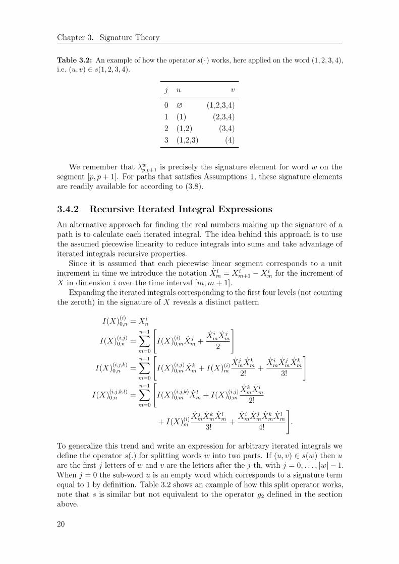
Table 3.2: An example of how the operator s(·) works, here applied on the word (1, 2, 3, 4),i.e. (u, v) ∈ s(1, 2, 3, 4).

j u v

0 ∅ (1,2,3,4)1 (1) (2,3,4)2 (1,2) (3,4)3 (1,2,3) (4)

We remember that λwp,p+1 is precisely the signature element for word w on thesegment [p, p+ 1]. For paths that satisfies Assumptions 1, these signature elementsare readily available for according to (3.8).

3.4.2 Recursive Iterated Integral Expressions

An alternative approach for finding the real numbers making up the signature of apath is to calculate each iterated integral. The idea behind this approach is to usethe assumed piecewise linearity to reduce integrals into sums and take advantage ofiterated integrals recursive properties.

Since it is assumed that each piecewise linear segment corresponds to a unitincrement in time we introduce the notation X i

m = X im+1 −X i

m for the increment ofX in dimension i over the time interval [m,m+ 1].

Expanding the iterated integrals corresponding to the first four levels (not countingthe zeroth) in the signature of X reveals a distinct pattern

I(X)(i)0,n = X i

n

I(X)(i,j)0,n =

n−1∑m=0

[I(X)

(i)0,mX

jm +

X imX

jm

2

]

I(X)(i,j,k)0,n =

n−1∑m=0

[I(X)

(i,j)0,m X

km + I(X)(i)m

XjmX

km

2!+X imX

jmX

km

3!

]

I(X)(i,j,k,l)0,n =

n−1∑m=0

[I(X)

(i,j,k)0,m X l

m + I(X)(i,j)0,m

XkmX

lm

2!

+ I(X)(i)mXjmX

kmX

lm

3!+X imX

jmX

kmX

lm

4!

].

To generalize this trend and write an expression for arbitrary iterated integrals wedefine the operator s(.) for splitting words w into two parts. If (u, v) ∈ s(w) then uare the first j letters of w and v are the letters after the j-th, with j = 0, . . . , |w| − 1.When j = 0 the sub-word u is an empty word which corresponds to a signature termequal to 1 by definition. Table 3.2 shows an example of how this split operator works,note that s is similar but not equivalent to the operator g2 defined in the sectionabove.

20


Under the assumed interpolation of n discrete measurements the signature of Xconsists of iterated integrals over the interval [0, n]. However any proof of a generalexpression for iterated integrals has to deal with the real valued times inside eachlinear segment, therefore the following theorem is formulated to hold for arbitrarytimes t.

Theorem 2. Let X : [0,∞)→ Rd be a path satisfying Assumption 1. Furthermorelet w = (i1, . . . , ik) be an arbitrary word with letters in the alphabet A = {1, . . . , d}.Then for any t ∈ [0,∞) with n = btc the iterated integral I(X)w0,t is given by

I(X)w0,t =n−1∑m=0

∑(u,v)∈s(w)

I(X)u0,m1

|v|!∏i∈v

X im

+∑

(u,v)∈s(w)

I(X)u0,n(t− n)|v|

|v|!∏i∈v

X in.

(3.12)

Proof. First we note that if t = n in (3.12) the second sum vanishes and

I(X)w0,n =n−1∑m=0

∑(u,v)∈s(w)

I(X)u0,m1

|v|!∏i∈v

X im

hence (3.12) can be written in a slightly shorter but equivalent form

I(X)w0,t = I(X)w0,n +∑

(u,v)∈s(w)

I(X)u0,n(t− n)|v|

|v|!∏i∈v

X in. (3.13)

Note that I(X)w0,n does not explicitly depend on t.To prove that these equations hold for any word w, induction over the word

length is used. The base case is a word of length 1, i.e. some single index i. For asingle letter word the split operator s will only produce one pair of sub-words whereu = ∅ and v = (i). Starting at the definition of an iterated integral and using thepiecewise linearity of X i

t we get that

I(X)(i)0,t =

t∫0

1 dX it =

t∫0

X it dt =

n−1∑m=0

m+1∫m

X it dt+

t∫n

X it dt.

Since X it is constant on each interval between two whole numbers it can be moved

outside the integrals and

I(X)i0,t =n−1∑m=0

X im

m+1∫m

dt+ X in

t∫n

dt =n−1∑m=0

X im +X i

n(t− n)

which shows that (3.12) holds when w = (i).For the induction step first assume that (3.13) (which is equivalent to (3.12))

holds for I(X)w0,t where w is a word with k letters. Add an extra letter j ∈ A to thisword to get w = (w, j) which has k + 1 letters. We now want to show that (3.12)

21


is fulfilled for w by using the inductive assumption. The definition of the iteratedintegral corresponding to w can be expanded into

I(X)w0,t =

t∫0

I(X)w0,t dXjt =

t∫0

I(X)w0,tXjt dt

=n−1∑m=0

Xjm

m+1∫m

I(X)w0,t dt+ Xjn

t∫n

I(X)w0,t dt = (I) + (II).

The terms (I) and (II) will be expanded independently. Starting with (I) wereplace I(X)w0,t according to the induction assumption which leads to

n−1∑m=0

Xjm

m+1∫m

I(X)w0,t dt

=n−1∑m=0

Xjm

m+1∫m

I(X)w0,m +∑

(u,v)∈s(w)

I(X)u0,m(t−m)|v|

|v|!∏i∈v

X im

dt

=n−1∑m=0

Xjm

I(X)w0,m

m+1∫m

dt+∑

(u,v)∈s(w)

I(X)u0,m

m+1∫m

(t−m)|v|

|v|!dt∏i∈v

X im

.

The integrals in this expression are computed by a change of variable

m+1∫m

(t−m)|v|

|v|!dt =

1∫0

s|v|

|v|!ds =

1

(|v|+ 1)!.

Thus

n−1∑m=0

Xjm

m+1∫m

I(X)w0,t dt

=n−1∑m=0

I(X)w0,mXjm +

∑(u,v)∈s(w)

I(X)u0,m1

(|v|+ 1)!

∏i∈v

X im

Xjm

=

n−1∑m=0

∑(u,v)∈s(w)

I(X)u0,m1

|v|!∏i∈v

X im

(3.14)

where in the final step the term outside the sum over s(w) and the factor Xjp is

absorbed when instead summing over s(w).

22


Similarly, the term denoted by (II) can be manipulated into

Xjn

t∫n

I(X)w0,t dt

= Xjn

t∫n

I(X)w0,n +∑

(u,v)∈s(w)

I(X)u0,n(t− n)|v|

|v|!∏i∈v

X in

dt

= XjnI(X)w0,n

t∫n

dt+ Xjn

∑(u,v)∈s(w)

I(X)u0,n

t∫n

(t− n)|v|

|v|!dt∏i∈v

X in

where the integrals are computed as before, yielding

t∫n

(t− c)|v|

|v|!dt =

t−n∫0

s|v|

|v|!ds =

(t− n)|v|+1

(|v|+ 1)!.

Resolving the integrals and once again absorbing extra terms into a sum over s(w)gives

Xjn

t∫n

I(X)w0,t dt

= I(X)w0,n(t− n)Xjn +

∑(u,v)∈s(w)

I(X)u0,n(t− n)|v|+1

(|v|+ 1)!

∏i∈v

X in

Xjn

=∑

(u,v)∈s(w)

I(X)u0,n(t− n)|v|

|v|!∏i∈v

X in.

This, when combined with (3.14), means that

I(X)w0,t =n−1∑m=0

∑(u,v)∈s(w)

I(X)u0,m1

|v|!∏i∈v

X im

+∑

(u,v)∈s(w)

I(X)u0,n(t− n)|v|

|v|!∏i∈v

X in,

recognised as the formula we want to prove, which means that the induction stepholds and the proof is complete.

The previous theorem shows that it is possible to calculate any iterated integralof X by starting with single letter words and iteratively calculating more and morecomplex iterated integrals. The sum over m indicates that is it not sufficient toonly know the lower order iterated integrals on the entire interval [0, n], one has toknow all n− 1 partial iterated integrals on the intervals [0,m] for m = 0, . . . , n− 1.Since in practical applications, the signature up to a real valued time t is not of anyinterest, we formulate a corollary which only concerns iterated integrals over wholenumber intervals.

23


Corollary 3. Let X : [0, n+ 1]→ Rd be a path satisfying Assumption 1. Then foran arbitrary word w = (i1, . . . , ik) with letters in A = {1, . . . , d} the iterated integralI(X)w0,n+1 is given by

I(X)w0,n+1 = I(X)w0,n +∑

(u,v)∈s(w)

I(X)u0,n1

|v|!∏i∈v

X in.

Proof. Follows directly from (3.13) since t = n.

With this corollary it becomes evident that a program which calculates signatureelements can do so by looping over a finite set of words and over the segments of thepiecewise linear path.

3.4.3 Log Signatures

The log signature of a path can be calculated from a signature first by (3.4) andthen (3.7). The only details missing in this computation is how to retrieve the set ofLyndon words L. While the set of Lyndon words is infinite, practical applicationsmust put a limit to the number of levels in a log signature. Such a truncated setof Lyndon words up to a certain word length k can be calculated with Duval’salgorithm [22,23]. The exact procedure is described in Algorithm 1.

Notation :Let w−1 denote the last letter of the word wInput :n ∈ Z+ – maximum Lyndon word length

d ∈ Z+ – alphabet sizeOutput :Ln – A set of integer tuples corresponding to all Lyndon words of

up to length n based on the alphabet {1, . . . , d}1 Ln = ∅2 w ← (0)3 while |w| > 0 do4 w−1 ← (w−1 + 1) mod d // Increment last digit5 Ln ← Ln ∪ {w} // Now w is a Lyndon word6

7 w ← www . . . // Repeat w8 w ← (w1, . . . , wn) // Trim to length n9

10 while w−1 = d and |w| > 0 do11 w ← (w1, w2, . . . , w|w|−1) // Remove trailing d’s12 end13 end

Algorithm 1: A procedure for generating a finite list of Lyndon words on thealphabet {1, 2, . . . , d}, based on Duval’s algorithm [22].

24

Chapter 4

Feature Extraction

In many applications of signal processing and data analysis, raw data is often difficultto make use of. For example sound data is sampled thousands of times per second.This means that a raw data sample is extremely high-dimensional. Furthermore, noisecan distort the signal and translation issues occur since samples are not necessarilyaligned in time. Data preprocessing is necessary in order to avoid these issues andextract usable information. The goal of preprocessing is to extract a set of so calledfeatures from a raw sample, expressing properties of the sample.

When dealing with sound as raw data, there are several options for featureextraction. In speech recognition [6] as well as language [4,24] and dialect classification[25], the most prominent technique involves Mel-frequency cepstral coefficients(MFCCs) which are based on the idea of mimicking human hearing.

In this thesis we will work with MFCCs and a closely related feature representationcalled Mel-frequency spectral coefficients (MFSCs). Furthermore, we also investigatethe possibility of using signatures, both as a stand-alone feature and as a dataenhancing compliment to other features.

4.1 Short-Time Fourier Transform

Given an audio signal, we are interested in the frequencies contained in the sampleand how these change over time. The short-time Fourier transform (STFT) computesthe frequency spectrum of a small time interval window, moving through the signal.This produces a spectrogram that provides us with an overview of how the frequenciesevolve throughout the speech sample.

The window size is set to 25 ms, with the assumption that human speech isstationary on a short time interval [26]. Before calculating the Fourier transform of awindow frame, however, the frame should be smoothed using some window functionto avoid artifacts arising from the edges of the window. A common window functionis the Hamming window, which is also the function of choice in this thesis. It is theweighted cosine with coefficients given by

wn = 0.54− 0.46 cos

(2πn

L− 1

), 0 ≤ n < L

with L being the window size. This function ensures that the signal vanishes towardsthe edges of the window. To make up for the fact that this causes loss of informationnear the edges, the window frames are made to overlap by 15 ms. After application

25

Chapter 4. Feature Extraction

of the window function, we calculate the frequency spectrum F (x) by discrete Fouriertransform. Letting the signal in a window be x = (x0, . . . , xL−1):

F (x)k =L−1∑n=0

wnxne−i2πkn/L, k = 0, . . . , 2K − 2

where wn are the components of the Hamming window and 2K − 2 is the number offrequency bins used in the transform. Here we choose 2K − 2 = 512. All frequenciesabove the Nyquist frequency are discarded, which for a 16kHz sample rate is 8 kHz.This leaves us with K = 257 actual frequency bins. The transformation is doneusing fast Fourier transform, and the result of the STFT is a spectrogram whereeach column contains the frequency spectrum of its respective time frame.

0 10 20 30 40 50Time frames

0

1

2

3

4

5

6

7

8

Freq

uenc

y [k

Hz]

Fourier Spectrogram

Figure 4.1: Fourier spectrogram. The figure shows logarithm of the pixel values forillustrativ purposes.

4.2 Mel-Frequency Spectral Coefficients

This section presents Mel-Frequency Spectral Coefficients, or MFSCs. The first stepis to calculate a frequency spectrogram by transforming the raw signal through STFT.In the second step, we use a Mel scale filter bank. The Mel-scale is a non-linearfrequency scale that mimics human hearing [27]. The human ear has finer frequencyresolution at lower frequencies and the Mel scale aims to be linear in terms ofhuman perception, rather than in actual frequency. The Mel-frequency relates to thestandard frequencies according to the relation

m = 2595 log10

(1 +

f

700

). (4.1)

The Mel-scale filter bank consists of a set of overlapping triangular filters, withcenters equidistantly spaced in the Mel-scale of (4.1). From a discrete and uniform

26


frequency range (0 = f0 < . . . < fK = 8000), we compute the corresponding discreteMel-frequency range using (4.1) and then place the filters uniformly on this range asseen in Figure 4.2, where 15 filters were used. The Mel-scale ensures that the filtersare more densely distributed at lower frequencies, and that they grow farther apartand wider at higher frequencies.

0 1000 2000 3000 4000 5000 6000 7000 8000Frequency [Hz]

0.0

0.2

0.4

0.6

0.8

1.0

15 filters

Figure 4.2: Mel-scale filter bank with 15 filters.

Given a speech sample x ∈ RN , we begin by computing the correspondingspectrogram, as done in Figure 4.1. Before applying a Mel filter bank however, eachcolumn in the STFT spectrogram is transformed into a power spectrum

Pk =1

L|F (x)k|2, k = 0, . . . , K

with K frequency bins. The result is a power spectrogram SP ∈ RK×T with K rowsrepresenting frequency bins and T columns, corresponding to the time frames.

The power spectrogram is then passed through a filter bank such as the onein Figure 4.2. Each filter is a function b : R → [0, 1], and a filter bank B with Ffilters is a matrix the rows of which will contain the set of uniformly discretizedtriangular filters. For each row i we have Bi = (b(i)(f0), . . . , b

(i)(fK). Thus, B is anobject in RF×K . Applying this filter bank to the power spectrogram produces a newspectrogram SMel ∈ RF×T :

SMel = BSP.

After transforming SMel to decibels, this yields the MFSCs, which are actually Mel-frequency spectrograms. Figure 4.3 shows an example of a Mel spectrogram for aperson saying the Swedish word dagar.

The number of filters in the filter bank determines the number of rows in thespectrogram. Figure 4.3 used F = 40 filters. Common values range from 20–40filters.

27


0 10 20 30 40 50 60Time frames

0

5

10

15

20

25

30

35

40M

el fr

eque

ncy

bins

Mel Frequency Spectrogram

Figure 4.3: Mel spectrogram of the word dagar from a dalarna dialect

4.3 Mel-Frequency Cepstral Coefficients

In a spectrogram each column is a frequency spectrum, or Mel spectrum, for aspecific time frame. This gives an overview of how the frequencies change throughoutthe sample. However, the frequency bins in the MFSCs are correlated, somethingthat is worsened by the fact that the filters in the filter bank are overlapping. Thisposes a problem for classification algorithms that uses covariance matrices, such asGaussian Mixture Models. Therefore, MFCCs proceeds one step further, in whichthe spectrogram is transformed using a discrete cosine transform (DCT), defined as

ck =N−1∑n=0

Xn cos

(πk

N

(n+

1

2

)), k = 0, . . . , N − 1

along each column, which decorrelates the rows.This also has the benefit of allowing us to discard the higher-order terms of

the DCT, without losing valuable information. These terms represent rapid, high-frequency changes in the Mel spectrum that carries little information about thesound. The lower-order terms instead correspond to the overall spectral shape, orspectral envelope. Thus, the DCT step can be thought of as a frequency analysis ofthe frequencies, known as cepstral analysis. Keeping only lower order terms, providesa smoother spectrum and a more dense representation. The result is a set of MFCCfeature vectors, as illustrated in Figure 4.4 where each column is a MFCC vector.

Not all classification techniques utilizes covariance matrices, however. Artificialneural networks can handle correlated samples, and convolutional networks are evenbased on the idea of local correlations within samples and so would benefit from thecorrelation. Therefore we will make use of both MFSCs and MFCC.

28


0 10 20 30 40 50 60Time frames

0

5

10

15

20

25

30

35

MFF

Cs

Mel-Frequency Cepstrogram

Figure 4.4: Spectrogram that has been decorrelated using a discrete cosine transform,hence a cepstrogram. The columns in the figure are MFCC feature vectors. Commonlyonly coefficients 0-12 are used, which means the other rows in the figure are discarded.

4.3.1 Shifted Delta Cepstra

While an MFCC sample does capture how a sound signal changes over time, webelow present classifiers which see each column in such a matrix as its own individualsample. Such classifiers are limited to finding properties of the signal which fits insidesingle time frames. To get around this restricted temporal context we will use amethod for expanding MFCC feature vectors with additional temporal information.

Temporal context is achieved by delta vectors [4], which express the change infeatures across neighbouring values. Let (x1, x2, . . . , xT ) be the column vectors in aMel-frequency cepstrogram with N cepstral coefficients. By letting xt = x1 if t < 1and xt = xT if t > T we indicate that the cepstrogram is extended at the left andright edges by repeating the first and last column respectively.

The classical definition for the delta features at time t with parameter n is∆xt = xt+n − xt−n which only utilizes the edges of the interval [t− n, t+ n] [28, 29].While this is a well-tested method we have opted for the alternative approach wherechange around xt is approximated using all neighbouring values [30]. The alternativedefinition of delta feature vectors is

∆xt =

∑nk=−n kxt+k∑nk=−n k

2for t = 1, . . . , T. (4.2)

This approach is perhaps most easily understood via linear regression. For eachtime t = 1, . . . , T we define a linear model

xt+k = α + βk + ek for k = −n, . . . , n

where α is intercept, β is slope and ek are residuals. The aim is to approximate βand use that approximation as our delta feature vector for time t. Note that while all

29


terms in the linear model are vectors, the regression is done for each component ofthe vectors, independently. Using least squares to find our approximations producethe slope estimate ∑n

k=−n(k − k)(xt+k − x)∑nk=−n(k − k)2

where the bar notation indicates an average over k = −n, . . . , n. Since k = 0 thisreduces to (4.2).

Now it is possible add temporal information to each MFCC feature vector xt byconcatenating it with its corresponding delta vector ∆xt. This would result in Tfeature vectors of length 2N . This can be taken a step further by applying the aboveprocedure to ∆xt instead of xt, resulting in delta-delta vectors and combined featurevectors of length 3N .

Here however, Shifted Delta Cepstra (SDC) [28,29] which is a generalization ofthe delta and delta-delta methodology are used. In SDC multiple delta featuresfrom shifted time positions are concatenated, providing temporal context. SDCfeatures are based on the delta vectors, meaning that we have both xt and ∆xt fort = 1, . . . , T calculated with parameters N and n respectively. The parameter Pdenotes the difference in time index between each shifted delta vector and k denoteshow many delta vectors will be picked out and concatenated for each time-frame.Finally the SDC vector at time t is the concatenation[

∆Tt ,∆

Tt+P ,∆

Tt+2P , . . . ,∆

Tt+(k−1)P

]T.

Combining MFCC and SDC vectors by yet another concatenation results in the finalMFCC + SDC feature vectors, each containing (k + 1)N elements.

4.4 Log Signatures as Acoustic Features

When incorporating signatures into dialect classification we have focused on logsignatures, since it has non-redundant coefficients and is smaller in size, which willaid classification methods. To calculate log signatures it is necessary that the inputdata can be seen as a path. A sound signal is sampled over time, and is thereforeinherently a path. Using amplitude as a single dimensional path however is not anoption, since the log signature of a path in R consists of just one element (due toproperties of the Lyndon basis).

Instead we have focused on the interpretation of MFCC samples as paths. MFCCsamples are sequences of feature vectors with length N , corresponding to how manycepstral coefficients are kept. By interpreting each cepstral coefficient as a dimension,the sequence of feature vectors become a path in an N-dimensional space, from whichlog signature can be computed. In practice truncated log signatures are used, whichcontain elements up to some level `.

Log signatures calculated from un-normalized MFCC feature vectors are numeri-cally unstable, producing extremely large elements in higher levels. To remedy this,before the log signature is calculated for a path, all path elements are normalized tozero mean and standard deviation one.

30


To simplify classification on log signatures we step away from the formal powerseries notation

logS(X) =∑w∈L

λweσ(w)

and instead express the log signature as the vector

logS(X) = [λw1 , λw2 , . . .]

for a fixed ordering of Lyndon words {w1, w2, . . .} ⊂ L of length up to `. In bothnotations each λw is a feature which will vary depending on the sample to logsignature is calculated for.

4.5 Normalization

The last step when preparing data for classification is normalization, specificallyfeaturewise normalization, which is applied to extracted features. The desiredoutcome of featurewise normalization is a set of feature samples where the averageand standard deviation of every feature over the entire set is equal to zero and onerespectively.

If the feature samples are vectors where each index corresponds to some feature,as is the case with our log signature features, normalization is very simple. If allfeature vectors are gathered as columns in a matrix, the normalized feature vectorswould be the original vectors minus the row means and divided by the columnstandard deviations.

For the spectro- and cepstro-scopic features however, there are multiple mea-surements for each feature per sample, since each row corresponds to a spectral orcepstral feature. Therefore the statistics are the average and standard deviationof each row across all spectrograms or cepstrograms. The actual normalization issimilar to the vectorized case, each column in the sample matrices are shifted andskewed individually with the computed statistics.

31

Chapter 5

Classifiers

The classification problems formulated in this thesis are examples of what is calledsupervised classification which is a general procedure were classifiers are constructed(also called trained) from examples. The training is based on a set of samplesx1, x2, . . . , xN ∈ X (also called the training set) and their corresponding labelsY1, Y2, . . . , YN ∈ {1, . . . , D}. The specifics of the input space X depends on whichtype of features are used but the labels always indicate which class each samplebelongs to (or comes from).

A classifier is in this context just a function or method for performing the mapping

X → {1, . . . , D}

as accurately as possible. This accuracy is both in terms of the examples availablethrough the test data (samples and labels), and ideally, accurate in terms of datacollected in the future.

We will see that classifiers are often defined in terms of parameters, of which thereare two important categories. Hyperparameters are specified before training andstate, for example, how large the classifier is or how the training should be controlled.The other kind are simply parameters, sometimes called trainable parameters forclarity, and as this name suggest these are derived during training such that theintended mapping to predictions is accurate. A classifier or classification methodcan produce very different results depending on its hyperparameters. It is thereforea fundamental part of supervised classification to find suitable hyperparameters.

5.1 Gaussian Mixture Models

Gaussian Mixture Models (GMMs) are one of the standard approaches to identifi-cation tasks on speech data [31]. Their suitability arises from their capability toadapt to arbitrarily shaped density functions. As the name suggests the mixturecomponents in GMMs are normal distributions. The multivariate normal distributionin Rd with mean vector µ ∈ Rd and covariance matrix Σ ∈ Rd×d has the densityfunction

f(x; µ,Σ) =1

(2π)k/2|Σ|1/2exp

(−1

2(x− µ)TΣ−1(x− µ)

), x ∈ Rd,

where |Σ| denotes the determinant of Σ.

33

Chapter 5. Classifiers

A GMM is built up from a weighted sum of M Gaussian density functions, oftencalled components of the mixture model. Besides a mean vector and covariancematrix, each component is associated with a positive weight parameter w. The sumof all weight parameters is equal to one which means that the mixture model itself isa valid probability distribution on Rd. For brevity we introduce θ = {wi, µi,Σi}Mi=1

as the complete set of parameters in a single GMM. The density function of a GMMwith parameters θ is then given by

G(x | θ) =M∑i=1

wi f(x; µi,Σi), x ∈ Rd.

The most demanding operation in GMMs is the inverse of the covariance matrixwhich is present in every mixture components density function. To decrease computa-tional load we assume all covariance matrices to be non-zero only on their diagonals.While this is a pruning of which densities the GMM can mimic, the setback can becompensated by adding more mixtures [32, p. 75].

5.1.1 Training

Since a GMM is entirely described by its parameters, fitting a GMM to data isa matter of finding θ such that the density of the GMM resembles the unknowndistribution of which the data is presumed to be sampled from. Here this is achieved bymaximum likelihood estimation, i.e. finding parameters that maximize the likelihoodof the GMM given a set of training vectors X = {x1, . . . , xN} ⊂ Rd. The likelihoodfunction is

L(θ | X) =N∏n=1

G(xn | θ).

To this end the Expectation–Maximization (EM) algorithm is utilized. The algorithmis an iterative procedure applicable to a wide array of statistical models. In each stepmodel parameters are updated so that the model likelihood increases monotonically.In the case of GMMs there are fairly simple explicit expression for how to updateθ. Exactly how many iterations are needed for convergence depends on the initialparameters. While initialization of parameters can be done randomly, the implemen-tation used for GMMs in this thesis uses k-means clustering [33] (calculated withElkan’s algorithm [34]).

A two-dimensional example of what a GMM can look like post training is presentedin Figure 5.1. The figure also indicates that the enforced diagonality of covariancematrices is not an issue when a suitably large number of components is chosen. Theoverall shape of the data cluster is captured by the log-density function, which is theintended outcome.

5.1.1.1 k-means clustering

The goal with using k -means clustering for parameter initialization is to assign everyvector in X to a mixture component. Then wi, µi and Σi can be initialized based onthe vectors assigned to the mixture with index i.

34


0 5 10 15 20 25x

0

5

10

15

20

25y

Data points

0 5 10 15 20 25x

GMM components

0 5 10 15 20 25x

-29.

517

-29.51

7

-21.186

-21.186

-16.

222

-16.

222

-16.222

-12.668

-9.78

4

-7.437

-5.607

-5.607

GMM level curves

Figure 5.1: An example of how the distribution of cluster of data points in R2 can beapproximated with a GMM constructed with the EM algorithm.

In k -means clustering X is divided intoM non overlapping subsets, called clusters,C = {C1, C2, . . . , CM} so that the sum of variances from each cluster is minimized.This can be expressed as the optimization of finding C that minimizes the quantity

M∑i=1

∑x∈Ci

‖x−mi‖2.

Here ‖.‖ is the euclidean norm and mi is the mean of points in cluster i.After optimal clusters have been found the initial parameters for the mixture

component with index i are calculated as

w(0)i =

1

N

∑x∈Ci

1, µ(0)i = mi and (Σi)

(0)j,j =

1

N

∑x∈Ci

x2 −m2i for j = 1, 2, . . . , d.

5.1.1.2 EM algorithm

With initial parameters θ(0) = {w(0)i , µ

(0)i ,Σ

(0)i }Mi=1 in place the EM algorithm is used

to refine the parameters [32]. Iteration k of the algorithm begins by calculating theintermediary probabilities

P(k)i,n = f(xn; µ

(k)i ,Σ

(k)i ), for i = 1, . . . ,M and n = 1, . . . , N

which represent how probable it is that sample xn belongs to mixture i underthe model parameters θ(k). Then the next set of parameters θ(k+1) are computedaccording to the update rules

w(k+1)i =

1

N

N∑n=1

P(k)i,n , µ

(k+1)i =

∑Nn=1 xnP

(k)i,n∑N

n=1 P(k)i,n

35


and (Σ

(k+1)i

)jj

=

∑Nn=1 x

2nP

(k)i,n∑N

n=1 P(k)i,n

− (µ(k+1)i )2 for j = 1, 2, . . . , d.

Stopping conditions are implementation specific. In the package used here thealgorithm stops when the gain from updating parameters falls below a specifiedtolerance.

5.1.2 Classification

When using GMMs for supervised classification each class is represented by itsown GMM. For D distinct classes this will results in D different sets of parametersθ1, . . . , θD which are found when training using data from only the corresponding class.Then each GMM mimics the distribution of that specific category and prediction isthen a question of seeing which GMM agrees the most with the sample. Suppose asample is a collection of N feature vectors on the form X = {x1, . . . , xT} ⊂ Rd. Wedefine the average log likelihood for the GMM θ as

`(X | θ) =1

T

T∑t=1

logG(xt | θ)

which is a more robust measurement of how well the sample fits to the GMM thanthe regular likelihood, especially when the number of vectors per sample varies. Thepredicted class of the sample X is then the GMM with the highest average loglikelihood, meaning

Y = arg maxi=1,...,D

`(X | θi).

5.2 Artificial Neural Networks

A deep neural network consists of multiple layers of nodes, often referred to asneurons. Similarly to the neurons of the brain, these neurons can be activated andproduce a response upon receiving an input signal, modeled by some activationfunction.

Layers of neurons are linked together so that a signal can propagate forwardthrough the network. Each connecting link between neurons in two layers is associatedwith a weight and a bias. These weights and biases make up the parameters θ ofthe network. The purpose of an artificial neural network is to construct a modelof neuron layers, linked through various connection designs and operations, andadjust its parameters so that the network approximates the true distribution p(y|x).Thus, neural networks are layered models, and can be expressed as a composition1

of functions, mapping input x to output y as

y = (F (L) ◦ F (L−1) ◦ . . . ◦ F (1))(x),

where the F (1), . . . , F (L) are functions representing the neuron layers, which can beassociated with different designs and operations in order to build the desired type ofnetwork.

1The composition of two functions g(x), f(x) is written as (g ◦ f)(x) = g(f(x))

36


5.2.1 Network Building Blocks

The layered structure of feedforward neural networks means that as long as each layerproduces output in a space which is the input space of the next layer, different layerscan be combined in different orderings. This section lists the layers and operationsthat make up the networks used in this thesis.

5.2.1.1 Fully Connected Layer

The perhaps most basic type of layer is a fully connected, or dense, layer, in whichevery neuron is linked to every single neuron in the previous layer. Hence, twolayers ` and ` + 1 with n and m neurons respectively, are connected through aweight matrix W ∈ Rn×m and bias vector b ∈ Rm. In layer `, the neural networkcomputes the neuron activations h(`+1) ∈ Rm of the next layer through a functionH(`+1) : Rn → Rm such that

h(`+1) = H(`+1)(h(`)) = G(W (`)h(`) + b(`)

). (5.1)

G is a function that applies the so-called activation function g : R→ R component-wise, so that G(x) = [g(x1), . . . , g(xd)]

T .

5.2.1.2 Activation Functions

The activation function is a vital component of artificial neural networks. If gis chosen to be a non-linear function, this allows the network to learn non-linearproperties of the data. Common alternatives for g include sigmoid functions andtanh, as well as rectified linear units (ReLU) which are the activation function ofchoice in this thesis. A ReLU is defined as

g(x) = max(0, x). (5.2)

This function is non-linear, and have readily available derivatives which are usedwhen training networks. It is worth noting that (5.2) is technically not differentiablein x = 0, however in practice this is not an issue since x is unlikely to be exactly zero,and should it occur it is easily dealt with by defining the gradient to zero at x = 0.

5.2.1.3 Output Layer

As already stated, ReLUs are used for activations in this thesis. In the last layer ofa network, however, a different activation function is applied. As mentioned above,the final layer corresponds to the class associations. In order to help us make senseof the output, we apply a softmax function, which allows us to interpret the outputof the network as probabilities. The true distribution y = (y1, . . . , yD) will then bea one-hot representation, meaning that yd = 1 for a sample that belongs to classd, and all other elements in y will be zero, since a sample can only belong to oneclass. If o is the output of the network without any activation function, the softmaxfunction generates the final output y, corresponding to the probabilities of a sample

37


x belonging to class d through

yd =eod∑Dj e

oj, (5.3)

so that yd = P(Y = d|x) where Y denotes the random variable representing classlabels. The artificial neural network thus models the distribution p(y|x, θ), wherethe parameters θ are the weights and biases of the network.

5.2.1.4 Convolutional Layers

The layers in the network architecture in Figure 5.2 are called dense or fully connectedlayers, since each neuron is connected to all neurons in the previous layer. Hence, thenumber of parameters in deep fully connected network architectures grows extremelyfast as the complexity increases. Convolutional layers are a design that exploitslocal correlations in the input by convolving small filters with the input. In eachconvolutional layer a set of trainable filters, each with its own weights and biases,are swept across the entire input looking for patterns. While the filters are randomlyinitialized, they will be trained to search for patterns that are useful for classification.Such a setup greatly reduces the number of parameters in the model since the filtershave limited support and are small compared to the input, and the convolutionallows the filters to detect patterns anywhere in input, regardless of position.

During the convolution, the input x ∈ Rd is extended with zeroes around theedges, in order to maintain the dimensions, so that xi = 0 for i < 1 and i > d. Thisprocedure also means that we reduce a bias towards the center of the input, sincewithout this extension of zeros, elements near the edges of x would be included infewer filters. In the one-dimensional case for a convolution between an input vectorx ∈ Rd and a filter f ∈ RM , the convolution operation can be written as

(f ∗ x)n =M∑m=1

fmxn−m+µ, n = 1, . . . , d

for filter size M and where µ is an offset parameter that takes care of the padding soµ = M+1

2for M odd and µ = M

2for M even. Due to the padding procedure where x

is extended with zeros, we can maintain the dimension after the convolution so thatf ∗ x ∈ Rd.

The convolution can be generalized to any dimension. For x ∈ Rd1×...×dN , aconvolution with a filter f ∈ RM1×...×MN is defined as

(f ∗ x)n1,...,nN =

M1∑m1=1

...

MN∑mN=1

fm1,...,mNxn1−m1+µ1,...,nN−mN+µN .

with n1, . . . , nN running from 1 to d1, . . . , dN , respectively.A convolutional layer can and usually does contain multiple filters, that can be

taught to search for different patterns in the input. For a 2D-image input, a layermight for instance contain one filter that has learned to look for horizontal edges,another for vertical edges and a third could be searching for curved patterns. Each

38


filter in the layer thus give rise to individual outputs, called feature maps, and asthese filters sweep across the image they will produce a high activation when lookingon a subsection of the image that matches their specific patterns. After the filterconvolution, biases are added and finally an activation function is applied to producethe output of the convolutional layer.

For a two-dimensional input image x ∈ Rd×d, a first convolutional layer with N (1)

number of M -by-M filters will have a kernel W ∈ RM×M×N(1) , which is a tensor thatstores the filters of the layer. The layer will also have biases b ∈ RN(1)×d×d . For filtern, this layer produces feature map hn ∈ Rd×d, according to

hn = G (Wn ∗ x+ bn) , (5.4)

with Wn ∈ RM×M being the n:th slice of the kernel that represents filter n and bnthe bias of that filter. It is common to have a single bias term per filter, hence allcomponents in bn ∈ Rd×d will be identical.

The result of the first convolutional layer will be h ∈ Rd×d×N(1) . Hence, forsubsequent convolutional layers, the input will have another dimension determinedby the number of filters in the previous layer (the input layer could also have additionaldimensions, as is the case for RGB-images, for which the input is x ∈ R3×d×d). Ageneral convolutional layer with N (`+1) filters can thus be described by a functionKN(`+1) : Rd×d×N(`) → Rd×d×N(`+1) that applies (5.4) for all filters in the kernelW (`+1) ∈ RN(`)×M×M×N(`+1) :

h(`+1) = KN(`+1)(h(`)) =

G(W1 ∗ h(`) + b1)

G(W2 ∗ h(`) + b2)...

G(WN(`+1) ∗ h(`) + bN(`+1))

5.2.1.5 Max-Pooling

Max pooling is a downsampling technique that is often applied after a convolutionallayer. Feature maps are downsampled by only keeping the maximum value fromregions of the input. This type of non-linear downsampling is called max-pooling.While in general max-pooling can be done using k-by-k sized patces, a common setupin image applications is non-overlapping two-by-two max-pooling, which reducesthe image size by a factor of four by only keeping the max value of each 2-by-2patch. This reduction in data size is one of the reasons for max-pooling, as it makescomputations easier for subsequent layers. Another reason is that this providesa local translation invariance, since it will not matter where in the pooling patchthe filter has been maximally activated. In turn, this can help the network handlelocal noise and variations. Two-by-two max-pooling can be written as the functionP : Rd×d → Rd/2×d/2, with d ∈ N being even:

h(`+1)i,j = P (h(`))i,j = max

{h(`)2i,2j, h

(`)2i,2j+1, h

(`)2i+1,2j, h

(`)2i+1,2j+1

}.

39


5.2.2 Network Architectures

Using the building blocks of the previous sections, we construct two well-knowntypes of network architectures. The first is a more basic design and it uses only fullyconnected layers. The other type is the convolutional network design, which haveproven very successful in wide-spread applications.

5.2.2.1 Multi-layer Perceptrons

By stacking fully connected layers such as in Section 5.2.1.1, we map some inputfeature vector x from the first layer, through intermediate hidden layers, to an outputy. Such a network architecture is referred to as a multi-layer perceptron (MLP). AMLP network of L layers can thus be written as a series of function compositions

y = (H(L) ◦H(L−1) ◦ . . . ◦H(1))(x).

Figure 5.2 illustrates a MLP using two hidden layers and two output classes. Thenetwork maps an input vector x ∈ R4, through two hidden layers h(1), h(2) ∈ R5 to afinal output vector y ∈ R2, where each hidden layer performs the operation describedby (5.1).

Figure 5.2: Artificial neural network with four-dimensional input and two hidden layers,mapping to two output nodes. The arrows between the neurons show the structure of theconnections.

5.2.2.2 Convolutional Neural Networks

A convolutional neural network (CNN) are another type of network architecturewhich, logically, utilizes the convolutional layers described in Section 5.2.1.4. However,CNNs aren’t composed solely of convolutional layers. As mentioned, the activationsof the filters in a convolutional layer are called “feature maps”. These feature mapstells us if and where in the input the filters found their patterns. In this sense,

40


convolutional layers act like feature extractors, and therefore convolutional layers areusually followed by one or more fully connected layers, which perform classificationon the features and feature locations, as found by the convolutional layers. Anexample of a CNN architecture is shown in Figure 5.3. Using the building blocks ofoperations described in this chapter, the network in Figure 5.3 can be written as

y = (H ◦H ◦ P ◦K32 ◦ P ◦K32)(x),

with a flattening of the tensor after the second max-pooling layer. This is necessarywhenever a fully connected layer follows a convolutional layer, since the output ofthe latter is a set of 2D-feature maps while the fully connected layer disregards suchstructure and simply takes a flattened feature vector as input.

Figure 5.3: Example of a convolutional neural network architecture with two convolutionallayers with max-pooling layers between them. The final two layers of the network are fullyconnected layers.

5.2.2.3 Modular Neural Networks

The building blocks of artificial neural networks allows for some freedom in termsof network architectures. A plethora of options exists; multi-layered perceptrons,convolutional networks and recurrent networks are perhaps the most common types.The choice of network type depends on application and the nature of the data.However, in some cases, multiple types of input data could be available that does notnecessarily fit into a specific kind of network. A system looking to identify peoplecould make use of a modular network where a convolutional network extracts visualfeatures from images and another network processes audio such as voice samples. Amodular neural network architecture could then fuse these modules together as inFigure 5.4, for instance by simply concatenating their output into a single vectorand then proceed with the concatenated vector for classification.

41


Figure 5.4: Modular network setup for a case when two different types of input areavailable. Module A and B process different inputs, and their outputs are concatenatedand fed to a decision module that performs classification.

5.2.3 Training

Once a network has been designed, we want to modify the weights and biases ofnetwork in order to learn a good approximation of the true distribution p(y|x). Thisprocess is known as training.

Letting y and y be the true and predicted label distributions for all samplesx1, x2, . . . , xN in our the data set that we will use to train our model, we begin bydefining our cost function as the cross entropy error function

C(θ;y, y) = − 1

N

N∑i=1

∑d

y(i)d log(y

(i)d ), (5.5)

where i denotes a sum over all N samples in the so-called training data set. The crossentropy has several properties that makes it an attractive choice as cost function.Since y(i)d and y(i)d are probabilities, C is always positive, and will give a high cost ify(i)d is small when y(i)d = 1. Furthermore, this cost function will give zero cost only ify exactly equals y. Even if the network were to predict the correct label for a sample,a cost would be present unless the prediction was done with 100% confidence, i.e.y(i)d = 1. This means that the cross entropy cost function can distinguish between anetwork that predicts the correct labels with high margin and one that just barelymade the right guess. The logarithm in (5.5) always defined, since the network willnever hypothesize that a class has zero probability thanks to the softmax function(5.3) in the output layer.

We are now looking to adjust the weights, filters and biases that constitute θ inorder to minimize the cost function for our training set. The gradients ∇θC can be

42


be found through the so-called backpropagation algorithm, in which we find gradientsby chaining partial derivatives of the cost function w.r.t all trainable parameters θin the network, such as ∂C

∂W (`) and ∂C∂b(`)

. The cost can then be minimized using somegradient descent method. Unfortunately, computing the full gradient is in practicevery expensive. The cost function (5.5) contains all samples in our training dataset, so finding the full gradient would require us to feed our entire data set throughthe network, which is infeasible in many applications due to the size of data sets.The solution is the stochastic gradient descent method, where the cost function isapproximated by the cost C of a small batch of randomly chosen samples with labelsyb, yb:

C(θ;yb, yb) = − 1

B

B∑i=1

∑d

y(i)d log(y

(i)d ), (5.6)

where B is the size of the batches, chosen so that B << N . This circumvents theneed for repeatedly going through a large training set at every step, and also providesstochasticity that helps the optimization escape local optima. During training,batches are continuously fed to the network. A full sweep of data set, i.e. the entiredata set has been passed to training, is referred to as an epoch. During training, itis common to perform several epochs in order to reach high performance.

For training, we use the Adaptive Moment Estimation (Adam) algorithm [35],which is a stochastic gradient descent technique. The name stems from the fact thatit utilizes an adaptive learning rate based on past gradients from previous iterations.Given the gradient gt = ∇θC(θt−1;y, y) at iteration t, the Adam algorithm calculatesfirst and second moments mt and vt as

mt = β1mt−1 + (1− β1)gt, t ∈ N (5.7)vt = β2vt−1 + (1− β2)g2t , t ∈ N (5.8)

where β1 and β2 are hyperparameters of the algorithm. Adam then updates theparameters θ with some learning rate α, according to the update rule

θt = θt−1 − αmt√vt + ε

, t ∈ N (5.9)

The number ε is a small constant included for numerical stability. The moments mt

and vt are bias-corrected versions of mt and vt, for details see [35].The update (5.9) is a combination of the current gradient and previous updates.

The moments counteract oscillations in the path of convergence by providing aninertia that drags the updates in the directions of gradients from earlier time steps,which leads to faster convergence.

5.2.3.1 Regularization

One of the major issues with artificial neural networks is their proneness to overfit tothe training data, which gives poor generalization abilities. This is explained in moredetail below but in short a network which performs too well on the training datamight not be the best network overall. To combat this, regularization techniques areapplied to networks, or components in networks.

43


One such technique is L2-regularization, which can be applied to some or allparameters (weights and biases) in a network. The regularized parameter’s L2-penalty is added to the cost function to discourage the network from growing toolarge parameters. If some subset of the parameters in a network θr ⊂ θ are L2-regularized this means that the cost function (5.6) is changed to

C(θ;yb, yb) = − 1

B

B∑i=1

∑d

y(i)d log(y

(i)d ) + α||vec(θr)||2,

where θr, which contains all L2-regularized weights matrices and filters, is flattenedto a vector its norm added as a penalty term. The influence of the penalty iscontrolled through the parameter α. This is to keep individual filters or weights fromdominating the output of the network, which counteracts overfitting.

Dropout [36] is another form of regularization where neurons in a network arerandomly dropped during training. Neuron dropping is controlled by the drop rateP(d) ∈ (0, 1) which can be specific for each layer or even each neuron. The droppingof neurons occur at the start of each batch, and the output of all dropped neuronsare then fixed at zero. After parameters have been updated all neurons are broughtback online, then a new set of randomly selected neurons are dropped for the nextbatch. This forces the network to train on randomly selected sub-networks of itself ateach iteration, which again keeps individual features or weights from dominating thedecision process. During evaluations of the network, however, the network shoulduse all its capacity and so all neurons are made available once training is complete.

44

Chapter 6

Experiments

In this chapter we present and explain the implementations for experiments outlinedin Section 2.3. There are three main categories of experiments: hyperparametercalibrations for single word classifiers, construction of multi-word classifiers andlastly testing the performance of a classifier trained with single word utteranceson spontaneous speech. Before the details of each experiment are given, someprerequisites are presented.

6.1 Generalization

When performing classification with trainable models, one of the most importantgoals is to construct a model which can accurately classify data it has not seen before.This is the concept of generalization. To test generalization it is necessary to refrainfrom training classifiers on all available data and instead set aside some data forevaluation, emulating the concept of unseen data. Similarly, any pre-processing stepswhich involve aggregated information about the data, such as normalization, is onlycalculated from training data, but applied to all data.

Furthermore, when the performance of multiple versions of a classifier (differingin hyperparameters) are compared, the winner’s accuracy will have a selection bias.Essentially the classifier which performs the best on the held out data, might do sobecause of some intrinsic property of that specific evaluation set.

Thus it is necessary to further split the data, setting aside yet another set which thewinning model can be evaluated on, producing a fair performance estimate. In total,data is split into three sets: training which is used when training classifiers, validationused for comparing their performance, and testing which accurately measures theperformance of the model with the best validation performance. All splits are maderandomly. Here a typical 70% for training and 15% for validation and testing each isused if nothing else is specified.

In all different experiments of this thesis, there are multiple samples coming fromthe same speaker. For example in single word experiments each subject leaves onaverage five utterances of each word. Therefore it is necessary that all splitting ofthe data is made based on speakers and not samples, meaning that all samples froma speaker must be in the same subset (training, validation or testing). If a certainspeaker has samples present in both training and evaluation sets, the properties oftheir speech is not strictly unseen and result will be skewed.

45

Chapter 6. Experiments

6.1.1 K-Fold Cross-Validation

One problem when splitting data in this fashion is that the outcome, i.e. the testaccuracy, is dependent on which data happened to be chosen as test data. If aparticularly difficult or simple sample ends up in the validation or test set, it mightskew the results.

K-fold cross-validation is a method for mitigating this variance dependent onsplits. Instead of just splitting data once, the data is randomly divided into k subsets.One at a time, the subsets take turns being the evaluation set, with the other k − 1subsets making up the training set. This means every sample will be in the evaluationset exactly once, and the average of the validation performance for all k folds is amore robust performance measure. This procedure is most commonly used after atesting set has been set aside and the remaining data is to be divided into trainingand validation. But one can also go a step further and cross-validate the test setand the validation set, as a sort of nested k-fold cross-validation.

6.2 Metrics

To measure performance of trained classifiers we employ the accuracy score as metric.A trained classifier can map a set of samples x1, . . . , xN to either predicted labelsY1, . . . , YN or predicted class densities y1, . . . , yN . If a classifier produces densitieswe pick the most probable class as the prediction by

Yi = arg maxd=1,...,D

yi,d for i = 1, . . . , N.

The accuracy score of the classifier on the dataset is then the percentage of correctlypredicted labels

100

N

N∑i=1

IYi=Yi .

When predicting class labels, every error will, from the point of view of a classd, be interpreted in one of two possible ways. Either a sample that is of class d ispredicted to be of some other class, called a false negative, or a sample which isnot in class d is mistakenly predicted as such, called a false positive. To quantifythese errors we introduce the metrics recall and precision, which we express usingthe indicator function I.

The recall of a classifier with regards to class d is the proportion of samples incategory d that are also classified as d, given by∑N

i=1 IYi=Yi=d∑Ni=1 IYi=d

.

As such recall puts a number on how well the classifier covers all samples from the dcategory.

Precision on the other hand quantifies the false positives of the classifier withrespect to some class d. It is defined as∑N

i=1 IYi=Yi=d∑Ni=1 IYi=d

46


which is the proportion of samples predicted as class d that are truly belonging toclass d. A high precision would indicate that samples assigned the label d most likelyactually belongs to that class.

6.2.1 Confusion Matrix

The confusion matrix is a way of visually illustrating the precision and recall for aclassifier regarding all classes at the same time. It also shows exactly which classesare mistaken for each other by the classifier.

In a classification problem with D classes the confusion matrix is a D×D matrixwhere rows indicate the true label of samples, and columns indicate predicted labels.Each element Ci,j in a confusion matrix is how many samples from class i werepredicted to be from class j. On this form a perfect classifier would only be non-zeroon the diagonal.

We define the normalized confusion matrix as the confusion matrix but normalizedsuch that each row sums to 1. The normalization means that if an element on thediagonal is equal to one, then all samples from that class are predicted to be inthat class, indicating perfect recall. However samples from other classes could bemistakenly predicted as belonging to this class as well, meaning precision is notnecessarily perfect in this case.

6.3 Single-word Calibration

As stated above the calibration of each classifier to single word dialect classificationis done by focusing on one of the calibration words dörr, flytta, kaka and lär at atime. For each word all utterances available in the wordlist data is extracted withinformation about speaker id. and dialect. All utterances shorter than one frame(25ms) were discarded since they cannot be used to construct features. On theother end all samples longer than 2 seconds were discarded since they were found tooften contain irrelevant additional sound bedsides the sought after calibration wordutterance. For each of the calibration words there are around 1400 samples.

To mitigate the variance in test accuracy 5 fold cross-validation is employed,creating five non overlapping test sets. The remaining data in each fold is thensplit once more into five, where each fifth takes turns being the validation set. Theremaining four subsets in the inner splits are training data. Each hyperparametercombination of a classifier is fit and evaluated on the five training and validationdata pairs. From this an average accuracy on the validation sets is obtained for eachhyperparameter combination, and the best one indicates the winner. This wholeprocedure is then repeated for all five test folds, producing five (possibly different)winning setups.

For each classifier, an overall winner is picked manually based on either mostfrequent wins or consistently high ranking among all five folds. The average per-formance of this calibrated version of each classifier on the test folds can then beused to compare the classifiers. Some of the classifiers do not need the validation setduring training, therefore their calibrated winners are trained on the remaining datain each test-fold, i.e. no splitting to training and validation sets.

47


6.4 Multi-word Classification

To construct multi-word ensemble classifiers we reuse the optimal setup of eachclassification method as per the calibration described above. The procedure is thesame for all classifiers: for each of the 43 wordlist words an independent calibratedclassifier are trained on samples of only that word, which is extracted in the samefashion as for the calibration words. Then an ensemble classifier which uses thepredicted class probabilities from multiple single word classifiers is constructed.Which single word classifiers to include is decided by forward selection.

The major difference between a single- and a multi-word classifier is that thelatter takes an n-tuple of input samples, one for each of the n internal single wordclassifiers it consists of. Our implementation of a multi-word classifier predicts labelsby sending each sample in the input tuple to the corresponding internal single wordclassifier. This produces n different class distributions that are merged by summationand the predicted label for the input tuple is then the argmax of the sum. Thisprocedure is straightforward for neural networks, which use a softmax activation toproduce output in [0, 1]D. When GMMs are used in multi-word classifiers they areredefined to instead output the average log likelihood of each internal distributiongiven the sample, which can be summed in the same manner as a density.

6.4.1 Splitting

While the single word classifiers used as building blocks in the multi-word classifierare trained independently (and therefore can be done in parallel), evaluation ontesting and validation data must be done with n-tuples of input samples. Exactlywhich words will be included is needs to be set beforehand, since it is necessaryto be able to evaluate the classifier using all 43 words. For this to be possible thevalidation and test sets must be constructed so that for every speaker, at least onesample for each of the 43 words is present.

Therefore the validation and test sets are constructed around speakers ratherthan samples, so that each item in either set consists of utterances for all 43 wordsfrom a single speaker. In Table A.1 we see that there are not enough speakers inthe data uttering all 43 words to enable folded cross-validation, for example in theJämtland dialect only 33% of speakers have uttered all 43 words at least once. Butthere are enough speakers uttering all words for a static split with 15% validationand 15% test data. In fact there are a large enough subset of speakers uttering allwords at least twice, meaning we can construct evaluation sets for the multi-wordclassifiers as follows.

For each dialect, approximately 30% of the number of speakers are selected fromthe speakers with at least two samples per word. These are divided evenly intotest and validation speakers. This selection and division of speakers is performedexactly once and every multi-word simulation loads the same division. This stopsany variance in results from including different people in validation/testing betweensimulations.

From this, test and validation sets are constructed so that for each speaker, twoseries of all 43 words are randomly sampled without replacement from their available

48


utterances. The limiting of each speaker only supplying two utterances per wordis to keep a balance between dialects and speakers. This sampling of utterances,together with the stochasticity in classifier training, introduces randomness betweensimulations and some variance is expected between runs for multi-word classifiers.

Lastly the training sets are specific to each word, and therefore is unaffected ifutterances for all 43 words aren’t available for some speakers. There are 43 sets oftraining data, each one containing all utterances of a word except those coming fromspeakers selected for testing or validation. These training sets are what is used toinitialize and train all 43 single word classifiers. Then comes the question of how tobest combine them.

6.4.2 Forward Selection

To select an optimal subset of words for dialect classification we implement forwardselection. For this we define two sets of words: W+ which is initially empty, whichholds the words added to the multi-classifiers and W− which holds the words not yetadded to the classifier, initially containing all 43 words. We define A(W ) to be theaccuracy score of multi-word classifier using the set of words W . Forward selectionis the iterative procedure where in each step the word w ∈ W− maximizing

A(W+ ∪ {w})

is added to W+ and removed from W−. This will grow the set of words one wordat a time, and by saving the validation accuracy for the chosen set of words ateach iteration as ai where i goes from 1 to 43, we study how adding words affectsperformance.

To mitigate the mentioned randomness between runs this procedure is repeatedthree times for each classifier used as basis in multi-word classification. This means,that three times over, data is initialized, single word classifiers are trained, combinedthrough forward selection, and the best model is evaluated on the test set.

6.5 Spontaneous Speech Classification

As we saw in Table 2.2, some dialects do not have sufficient annotation coveragefor testing the performance on spontaneous speech. Therefore we restrict ourselfto only three dialects: Jämtland, Sydfinland and Skåne. In each of these dialectsaround 30% of speakers have an annotated spontaneous interview, which meansthey can be used in the test and validation sets for this experiment. These speakersare split randomly into testing and training. For each such speaker, all annotatedsound samples are extracted and trimmed if necessary to a maximal length of 10seconds. For the remaining 70% of speakers, all utterances of the 43 wordlist wordsare extracted and used in the training set.

Of course, this is an easier problem than a 7-way classification, and earlier resultswill not be comparable. To get a fair reference the calibrated classifiers are trainedand evaluated for each calibration word, using the same split of speakers as aboveon the 3-way dialect classification.

49

Chapter 7

Results

7.1 Hyperparameter Calibration

Here we present which classifiers are used with which features for dialect classifica-tion. We also identify which tuneable hyperparameters each classifier and featurecombination has.

7.1.1 Gaussian Mixture Models

As a dialect classifier, GMMs are combined with MFCC +SDC features. Thiscombination is henceforth referred to in short as GMM. As MFCC feature vectorsare coefficients of an orthogonal (cosine) basis, the assumption of diagonal covariancematrices made when defining GMMs is plausible. Of course the vectors might notbe perfectly decorrelated, depending on properties of the underlying data.

The varying length of samples is not an issue for a GMM classifier. In trainingall samples in each dialect are combined when constructing that dialect model. Andin prediction the average log-likelihood is insensitive to varying length.

The hyperparameters specifying this classifier are the number of componentsM in each dialect mixture model, and the quadruple (N, n, P, k) which states howMFCC and SDC vectors are generated, as explained in Section 4.3.1. A filterbankwith 20 filters were used when generating MFCC features. Table 7.1 shows whichvalues of hyperparameters were tested, all possible combinations of these were trainedand evaluation according to the nested folding procedure outlined above. The tablealso shows which hyperparameter setup performed on average the best. Most notablythe smallest number of mixture components performed the best, whereas in otherdialect identification studies 256 (and even up to 2048 when a lot of data is available)mixture components have been used [8]. Most likely this is due to utterances of singlewords makes up less complex distributions than spontaneous speech and thereforenot as many mixture components are needed. As indicated larger GMMs are alsomore common in situations where more data is available for training them.

7.1.2 Multilayer Perceptron

As a classifier for log signature feature vectors (based on MFCC paths) we havechosen a Multilayer Perceptron. The maximum log signature level is fixed to ` = 3and path dimension is fixed to N = 10. This results in vectorized log signatures that

51

Chapter 7. Results

Table 7.1: Tested hyperparameters when calibrating the Gaussian Mixture Model classifierfor single word dialect classification.

Parameter Values

M 64, 128, 256N 8, 10, 12n 1, 3, 5P 6, 10k 1, 2, 3

are elements of R385. During training the MLP uses 32 samples per mini-batch andall weights and biases are L2-regularized with the hyperparameter α.

In hyperoptimzation, network architecture, α and the number of training epochsare varied. Networks were designed so that the first hidden layer had 64, 128, 256and 512 neurons. All consecutive hidden layers then has half the amount of neuronsas the previous one. Following this pattern networks two, three and four layers deepwere constructed. Each network architecture was combined with all combinations ofα = 0.0001, 0.001, 0.01 and Nepochs = 100, 500, 1000 when evaluated according to thenested cross-validation scheme.

The results of this hyper-optimization were more inconclusive, with many differentnetwork architectures performing the best on different folds, although compared tothe other classifiers they all performed poorly. The network with two hidden layersof size 512 and 256 was chosen together with α = 0.001 and Nepochs = 500 to playthe role of calibrated multilayer perceptron.

7.1.3 Convolutional Neural Network

Convolutional neural networks are an extension of MLPs, and as such they have evenmore hyperparameters. Combined with longer training times, thorough parametersweeps are not feasible. Instead, a number of setups were chosen for testing.

The number of convolutional layers was varied from a single layer to threeconsecutive layers, followed by two or three fully connected layers. After eachconvolutional layer, a 2-by-2 max-pooling layer was implemented. Filter sizes of5-by-5, 10-by-5 and 5-by-10 were tested, and the number of filters in the convolutionallayers were either 64, 32 or 16. Initial learning rates of 0.0001 and 0.001 were tested.All networks were designed with L2-regularization on the fully connected layers, anda drop rate of 0.5 on all fully connected layers during training. All setups used ReLUactivation functions for all hidden layers.

Performances were similar for all tested designs.The network with two convo-lutional layers with 32 and 16 filters respectively, followed by two fully connectedlayers with 512 and 7 neurons, gave the highest accuracy.

52

Chapter 7. Results

Table 7.2: Average test set classification accuracy over 5-fold cross-validation on the fourcalibration words for hyperparameter-calibrated classifiers.

Classifier FeaturesCalibration word performance (avg. %)

dörr flytta kaka lär

GMM MFCC + SDC 61.3 60.3 61.4 55.7MLP Log signature 42.5 41.7 46.0 39.3CNN MFSC 55.4 56.3 58.7 49.7

Modular MFSC +Log Sig. 56.7 54.4 59.6 52.6

7.1.4 Modular Network

The modular network was not optimized for any parameters, partially due to timerestrictions but also the even larger number of parameters available to choose from.Instead, the structure was chosen from the winning convolutional neural networkalong with a MLP structure of two hidden layers with 256 and 7 neurons each.

Since the modular network contains more parameters than the winning convolu-tional network, dropout regulation was used not only on the fully connected layersbut also on the last convolutional layer.

7.2 Performance on Calibration Words

We now want to compare the performance of our calibrated classifier setups. It wasfound that performance of single word classification varied strongly between runs,depending on how data was split, which is the motivation for employing folded cross-validation. For example the test accuracy of the calibrated GMM varied between52.2% and 60.0% on the five folds.

The average accuracies over folds for calibrated classifiers are shown in Table 7.2.The Gaussian mixture models gave better performance than any of the networks,outperforming the convolutional neural network with 3–g6%. While the higheraccuracy of the GMM is consistent for all four words, the CNN and the modularnet are quite close. A reason for this could be that GMMs are well known and finetuned as a method, whereas CNNs are newer in this application and the optimalstructure of layers might not have been found. Furthermore, the CNN could alsosuffer more than the GMM from the relatively small amount of available data.

The multilayer perceptron, however, lagged behind the GMM on average by 17.3%over the four words. This large discrepancy among otherwise similar performancescould indicate that the log signatures passed to the MLP are not suitable for one-worddialect classification. A convolutional network based on log signatures is unlikely toperform better than the MLP since the log signatures do not contain local correlations,which CNNs is designed to capture.

Figures 7.1 and 7.2 show normalized confusion matrices from classification meth-ods based on utterances of the word kaka with a GMM and CNN respectively(numerical versions of these matrices can be found in Appendix A). The confusion

53

Chapter 7. Results

Norrb

otten

Jämtla

nd

Sydfin

land

Dalarn

a

Mälard

alen

Västku

sten

Skåne

Norrbotten

Jämtland

Sydfinland

Dalarna

Mälardalen

Västkusten

Skåne

GMM on kaka

0.0

0.2

0.4

0.6

0.8

1.0

Figure 7.1: Normalized confusion matrix for a Gaussian mixture model on the word kaka.

matrices are basically in agreement between the two classifiers. Both classifiers reachhighest precision and recall for Skåne, suggesting that this is the most distinguishabledialect. Also, Norrbotten and Jämtland have high confusion between them, which isin agreement with the dialect division done by Wessén as discussed in Section 2.2,where these two regions are considered to share the same dialect.

7.3 Multi-word Performance

In Table 7.2, the word lär yields significantly lower performance than the otherthree. This indicates that some words are more suitable than others for use in dialectclassification, which is the motivation behind multi-word classifiers.

Each of the four classifiers were implemented as root for an ensemble classifierover words. As mentioned the experiment was repeated three times for each classifierand moderate variance in results was observed. The average results are shown inFigure 7.3. It appears that using multiple words during classification significantlyimproves classification performance.

Most surprisingly, the multilayer perceptron combined with log signatures, whichhad the worst performance on calibration words, catches up with the other ensemblesin terms of validation accuracy. This behavior is similar to that of [4], where anaccuracy of 76.92% was reported for seven North American dialects (TIMIT) usingfive words, with the best one-word classifier reaching 41.35% accuracy.

Table 7.3 shows the average number of words picked by forward selection andthe average validation and test accuracy for the picked multi-word classifiers. Theresults suggests that the MLP classifier using log signature features benefit to ahigher degree from the information in multiple words. While the GMM performed

54

Chapter 7. Results

Norrb

otten

Jämtla

nd

Sydfin

land

Dalarn

a

Mälard

alen

Västku

sten

Skåne

Norrbotten

Jämtland

Sydfinland

Dalarna

Mälardalen

Västkusten

Skåne

CNN on 'kaka'

0.0

0.2

0.4

0.6

0.8

1.0

Figure 7.2: Normalized confusion matrix for a convolutional neural network on the wordkaka.

best on the test set, the difference in accuracy compared to the other classifiers isbarely significant. The GMM also required the fewest number of words, but againonly with a small margin except for the MLP.

All four classifiers benefit from the ensemble setup with multiple words, reachingthe best performance using around 15 words, after which accuracy actually startsdropping. This indicates that adding some words merely confuse the classification.While some words have higher individual accuracy than others, the forward selectiondoesn’t simply choose the best individual words, which means that it is not neces-sarily the words with the lowest individual accuracy on their own that causes thisdegradation. One run chose sitt as the fifth word, while leaving gata at 34:th place,despite the words having an individual accuracy of 42% and 61% respectively. Hence,word combinations seem to matter for the classifiers. This suggests that differentwords can carry complimentary information that is valuable for dialect classification.

Table A.3 shows the order in which the forward-selections chose each word,averaged over three runs for each classifier. The fact that three of the calibrationwords are in the top 9 most chosen words indicates that results can be skewed.Because the calibration words were used to tune the classifiers, they are unfairlyfavored. A more robust method for a multi-word classifier would not just train aclassifier for each word, but also tune it individually.

A normalized confusion matrix for a multiword classifier using GMMs can beseen in figure Figure 7.4 (again, a numerical equivalent can be found in Appendix A).Interestingly enough, Skåne is no longer the easiest dialect to classify, and theconfusion between Norrbotten and Jämtland is much less pronounced. A notabletrend here would be that many persons are incorrecly predicted to come from Dalarna.

55

Chapter 7. Results

0 10 20 30 40Number of words

0.50

0.55

0.60

0.65

0.70

0.75

0.80

0.85

0.90

Avg.

val

idat

ion

accu

racy

(%)

Forward selection over words

GMMMLPCNNBNET

Figure 7.3: Average validation set accuracy over three independent training runs forensemble classifiers combining multiple single-word classifiers via forward selection.

Table 7.3: Average classification accuracy and number of words selected over three randominitializations of multiword data.

ClassifierAverage forward select results

Num. of words Val. acc. (%) Test acc. (%)

GMM 12.0 88.6 80.1MLP 19.3 89.1 79.3CNN 14.3 84.9 78.0

Modular 13.7 87.4 79.7

56

Chapter 7. Results

Norrb

otten

Jämtla

nd

Sydfin

land

Dalarn

a

Mälard

alen

Västku

sten

Skåne

Norrbotten

Jämtland

Sydfinland

Dalarna

Mälardalen

Västkusten

Skåne

Multiword GMM

0.0

0.2

0.4

0.6

0.8

1.0

Figure 7.4: Normalized confusion matrix for a multi-word GMM using a forward selectedset of words.

7.4 Other Signature-based Implementations

During the course of this project, several signature-based implementations wereinvestigated, however, initial results were not promising. In [14], signatures werecalculated on moving windows along a path. Inspired by this, we implemented a short-time signature transform in combination with convolutional networks, analogouslyto the short-time Fourier transform in Section 4.1, but classification was very poor.

Signatures were also computed from MFSCs, rather than MFCCs as in the resultsabove, but yet again no increased performance was observed. Trials were run usingboth GMMs and MLPs. Signatures were investigated as a feature to provide temporalinformation for GMMs by replacing shifted delta-cepstra with log signatures. Pathsderived from lead-lag transforms [19] were attempted, but generally led to very lowclassification accuracy.

In [15] the path is divided into sub-paths, motivated by the idea that multiplesignatures with few levels capture more information than one single signature withmany levels. This was implemented in combination with MFCC features andconvolutional networks but did not surpass the performance of a single large signature.

7.5 Spontaneous Speech Classification

For the simplified problem of discerning the dialects Jämtland, Sydfinland and Skåne,the calibrated classifiers gained much higher accuracies. A calibrated GMM reachedclassification accuracies of 87.6% on dörr, 75.2% on flytta, 76.1% on kaka and 67.5%on lär. This is a significant gain in accuracy compared to the classification with

57

Chapter 7. Results

secen dialects, which is to be expected. All of these classifiers had test accuraciesthat were around 10% higher than their validation accuracies. This indicates thatthis specific split caused the test set to be easier, and highlights the importance offolded cross validation, which unfortunately is impossible with the current data.

When training a GMM on all 43 words, it is necessary to increase the number ofcomponents. Rudimentary hyperparameter optimization showed that 1024 mixturecomponents were suitable for this task, achieving a validation accuracy of 59.0%.The test accuracy for this GMM was 69.0%. While this is not on par with the singleword classifiers, it shows that there is at least some overlap in dialectal featuresbetween utterances of words and spontaneous speech.

7.6 Effect of Speaker Identity

As discussed in Section 6.1, the experiments in this thesis was conducted by dividingsamples in the data into training, validation and test sets based on speaker identity.However, the relatively low number of unique speakers leads to high variance inthe experiments, as accuracy can be heavily influenced by a difficult speaker beingpresent in the test or validation set. This suggests that the number of speakers isimportant to achieve decent classification.

In fact, speaker identity appear to be a very significant factor. During thisinvestigation, a single CNN was trained and evaluated on all 43 wordlist words.Classification on data splits that allows for samples from a particular speaker beingpresent in training, validation and test sets reached over 90% accuracy for sevendialects. While repeated utterances of the same word by the same speaker are verysimilar, as shown in the two upper panels in Figure 7.5, and therefore easily identifiedif such utterances are found in both training and test sets, such cases does not explainthe entire gain in accuracy. This was illustrated by an experiment in which dataagain was split so that we allowed the same speakers to be present in all three sets,but now restricted utterances of particular words to be present only in one set. Thisexperiment reached close to 80% for seven dialects, which suggests that the modelsmore easily picks up on speaker identity itself, even when it is exposed to words thatit has never encountered before.

In Figure 7.5, it is perhaps possible that the pronunciations of the vowel a, visibleas a tilted V -shape in the spectrogram, are similar for the samples from Speaker1 (all but the bottom right pane). Such local features could feasibly explain whyspeaker identity appears to be a dominating source of variance in our data set.

58

Chapter 7. Results

0 10 20 30 400

10

20

30

40Speaker 1: 'jaga'

0 10 20 30 40 500

10

20

30

40Speaker 1: 'jaga'

0 10 20 30 40 50 600

10

20

30

40Speaker 1: 'saker'

0 10 20 30 40 500

10

20

30

40Speaker 2: 'jaga'

Figure 7.5: Four word utterances. The two upper figures are from the same speakeruttering the word jaga. The bottom left is also from this speaker, uttering saker. Bottomright is again jaga but from a different speaker.

59

Chapter 8

Conclusions

The results of this thesis suggest that classification of Swedish dialects based onacoustic features is possible and can be done with similar performance as in otherlanguages. As the SweDia2000 project continues to annotate their database, it isnot unfeasible that future studies can also test this on entirely spontaneous data.Furthermore, state of the art dialect classifiers use combinations of the differentfeatures such as the lexical or prosodical features, whereas here only acoustic ones wereused. Such a pooling of information about samples will very likely push performanceeven further.

In this thesis we have only looked at dialect classification itself. It would be ofinterest to evaluate the intended boost in speech recognition performance in Swedishthat would come from tailoring automatic speech recognition methods for each dialect.Using such a system it would also be possible which dialects (and which formulationsof them) are distinct enough

While the established Gaussian mixture models and convolutional neural networkswere superior for single-word classification, the relatively simple feedforward networkapplied to the log signature of Mel-frequency cepstrums caught up in performanceas a multi-word classifier. This is both remarkable and suspicious, and may indicatethat a larger data set should be used to verify the result. Many different methods forincorporating signatures or log signatures into speech features were tested withoutsuccess, but the search has by no means been exhaustive. It is certainly possiblethat the optimal way of utilizing signatures is yet to be discovered.

Across the board, the experiments in this thesis has been formulated with theavailable data in mind. In the end, many experiments were on the edge of what isacceptable in terms of data size. It would therefore be of interest to expand thedialect regions, most likely resulting in more robust experiments. This would at thesame time decrease the margin between them, and depending on the outcome ofclassification on such regions, the idea of smooth transitions between dialects can betested.

61

Appendix A

Tables

63

Appendix A. Tables

Norrb

otten

Jämtla

nd

Sydfin

land

Dalarn

a

Mälard

alen

Västku

sten

Skåne

Norrbotten

Jämtland

Sydfinland

Dalarna

Mälardalen

Västkusten

Skåne

.57

.27

.00

.05

.05

.06

.01

.21

.55

.00

.10

.02

.10

.02

.00

.03

.65

.18

.11

.01

.01

.02

.04

.10

.53

.20

.04

.06

.02

.02

.03

.11

.72

.08

.02

.07

.11

.00

.09

.18

.50

.06

.01

.01

.00

.03

.05

.10

.80

GMM on kaka

Figure A.1: Normalized confusion matrix for the Gaussian mixture model on the wordkaka.

Norrb

otten

Jämtla

nd

Sydfin

land

Dalarn

a

Mälard

alen

Västku

sten

Skåne

Norrbotten

Jämtland

Sydfinland

Dalarna

Mälardalen

Västkusten

Skåne

.57

.33

.00

.00

.00

.07

.03

.15

.67

.00

.00

.03

.03

.12

.00

.09

.77

.09

.05

.00

.00

.04

.02

.16

.56

.20

.00

.02

.00

.02

.02

.14

.73

.09

.00

.04

.08

.00

.02

.20

.56

.10

.04

.00

.00

.06

.02

.10

.78

CNN on 'kaka'

Figure A.2: Normalized confusion matrix for the Convolutional network on the wordkaka.

64

Appendix A. Tables

Norrb

otten

Jämtla

nd

Sydfin

land

Dalarn

a

Mälard

alen

Västku

sten

Skåne

Norrbotten

Jämtland

Sydfinland

Dalarna

Mälardalen

Västkusten

Skåne

.77

.09

.00

.05

.00

.09

.00

.10

.70

.00

.00

.05

.15

.00

.00

.00

.80

.15

.05

.00

.00

.00

.00

.00

.96

.00

.04

.00

.00

.00

.00

.04

.96

.00

.00

.00

.00

.00

.09

.05

.86

.00

.00

.00

.00

.09

.00

.00

.91

Multiword GMM

Figure A.3: Normalized confusion matrix for a multi-word GMM using a forward selectedset of words.

Table A.1: The number of unique speakers in each dialect region as well as informationabout how many speakers in each dialect provides at least n utterances for every wordlistword.

DialectUniquespeakers

n = 1 n = 2 n = 3 n = 4 n = 5

Norrbotten 79 30 (38.0%) 24 (30.4%) 20 (25.3%) 16 (20.3%) 4 (5.1%)Jämtland 72 24 (33.3%) 24 (33.3%) 22 (30.6%) 17 (23.6%) 5 (6.9%)Sydfinland 70 33 (47.1%) 30 (42.9%) 28 (40.0%) 2 (2.9%) 0 (0.0%)Dalarna 87 43 (49.4%) 41 (47.1%) 32 (36.8%) 6 (6.9%) 0 (0.0%)Mälardalen 82 71 (86.6%) 71 (86.6%) 61 (74.4%) 6 (7.3%) 0 (0.0%)Västkusten 75 61 (81.3%) 60 (80.0%) 58 (77.3%) 28 (37.3%) 2 (2.7%)Skåne 75 62 (82.7%) 61 (81.3%) 60 (80.0%) 28 (37.3%) 2 (2.7%)

65

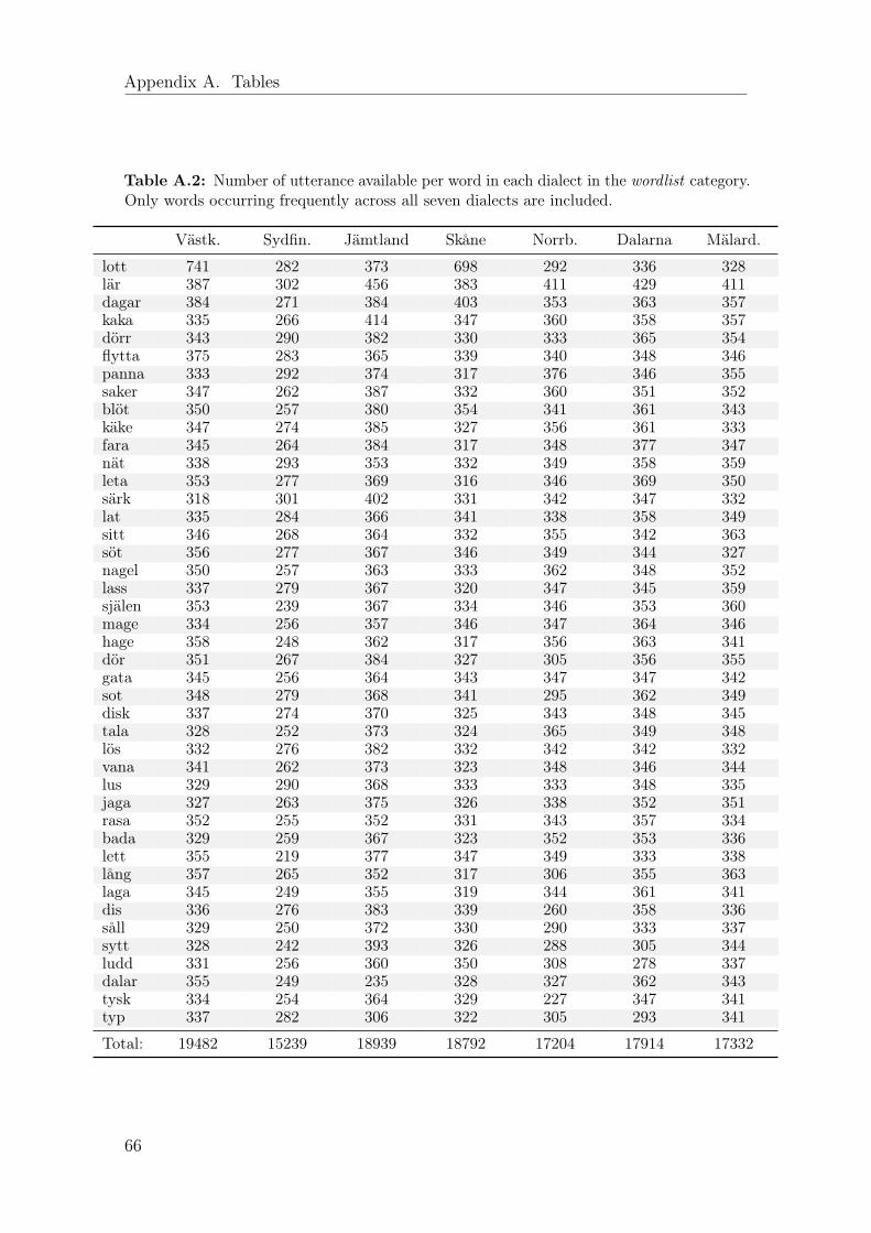
Appendix A. Tables

Table A.2: Number of utterance available per word in each dialect in the wordlist category.Only words occurring frequently across all seven dialects are included.

Västk. Sydfin. Jämtland Skåne Norrb. Dalarna Mälard.

lott 741 282 373 698 292 336 328lär 387 302 456 383 411 429 411dagar 384 271 384 403 353 363 357kaka 335 266 414 347 360 358 357dörr 343 290 382 330 333 365 354flytta 375 283 365 339 340 348 346panna 333 292 374 317 376 346 355saker 347 262 387 332 360 351 352blöt 350 257 380 354 341 361 343käke 347 274 385 327 356 361 333fara 345 264 384 317 348 377 347nät 338 293 353 332 349 358 359leta 353 277 369 316 346 369 350särk 318 301 402 331 342 347 332lat 335 284 366 341 338 358 349sitt 346 268 364 332 355 342 363söt 356 277 367 346 349 344 327nagel 350 257 363 333 362 348 352lass 337 279 367 320 347 345 359själen 353 239 367 334 346 353 360mage 334 256 357 346 347 364 346hage 358 248 362 317 356 363 341dör 351 267 384 327 305 356 355gata 345 256 364 343 347 347 342sot 348 279 368 341 295 362 349disk 337 274 370 325 343 348 345tala 328 252 373 324 365 349 348lös 332 276 382 332 342 342 332vana 341 262 373 323 348 346 344lus 329 290 368 333 333 348 335jaga 327 263 375 326 338 352 351rasa 352 255 352 331 343 357 334bada 329 259 367 323 352 353 336lett 355 219 377 347 349 333 338lång 357 265 352 317 306 355 363laga 345 249 355 319 344 361 341dis 336 276 383 339 260 358 336såll 329 250 372 330 290 333 337sytt 328 242 393 326 288 305 344ludd 331 256 360 350 308 278 337dalar 355 249 235 328 327 362 343tysk 334 254 364 329 227 347 341typ 337 282 306 322 305 293 341

Total: 19482 15239 18939 18792 17204 17914 17332

66

Appendix A. Tables

Table A.3: Average ranking of words in forward selection, sorted from best to worst overallranking. Blue rows indicate words used for calibration.

Word GMM MLP CNN BNET Overall

saker 1 15 2 3 5själen 9 2 2 11 6leta 15 5 17 12 12kaka 2 12 14 26 14flytta 11 19 9 15 14blöt 17 12 9 19 15disk 22 11 15 14 16dörr 10 17 24 14 17särk 7 9 28 23 17typ 15 26 18 8 17dör 28 2 23 15 17

vana 21 27 13 10 18rasa 13 24 16 21 19lat 9 22 35 11 19

lång 25 15 27 11 19lass 12 30 7 30 20lett 31 8 21 20 20hage 30 16 23 11 20dalar 7 29 26 18 20tala 30 6 23 23 21sot 16 15 26 25 21laga 33 20 17 14 21nagel 11 27 13 36 22gata 14 35 18 22 22lös 24 26 20 21 23dis 23 20 22 27 23

ludd 36 23 21 17 24fara 30 18 23 28 25lott 13 30 23 35 25

panna 35 25 27 18 26käke 29 16 29 33 27jaga 22 42 17 26 27bada 20 33 32 23 27nät 22 31 21 34 27

dagar 23 29 31 27 27mage 33 27 33 25 30sitt 32 32 27 28 30sytt 35 18 35 32 30lus 26 40 27 33 31söt 42 35 23 29 32lär 43 33 37 17 32såll 38 28 34 40 35tysk 30 34 38 39 35

67

Bibliography

1. A. Eriksson, Swedia recording locations, http://www.ling.gu.se/~anders/SWEDIA/kartor/Map.pdf, 2016, Online, accessed 2017-05-08.

2. H. Petkar, A review of challenges in automatic speech recognition, In-ternational Journal of Computer Applications 151 (2016), no. 3, 23–26,DOI: 10.1016/j.specom.2007.02.006.

3. F. Biadsy, Automatic dialect and accent recognition and its application tospeech recognition, Ph.D. thesis, Columbia University, 2011, URL: http://www.cs.columbia.edu/speech/ThesisFiles/fadi_biadsy.pdf.

4. M. Rizwan, B. O. Odelowo, and D. V. Anderson, Word based dialectclassification using extreme learning machines, Neural Networks (IJCNN),2016 International Joint Conference on, IEEE, 2016, pp. 2625–2629,DOI: 10.1109/IJCNN.2016.7727528.

5. N. F. Chen, W. Shen, J. P. Campbell, and P. A. Torres-Carrasquillo, Informativedialect recognition using context-dependent pronunciation modeling, Acoustics,Speech and Signal Processing (ICASSP), 2011 IEEE International Conferenceon, IEEE, 2011, pp. 4396–4399, DOI: 10.1109/ICASSP.2011.5947328.

6. S. A. Majeed, H. Husain, S. A. Samad, and T. F. Idbeaa, Mel frequency cepstralcoefficients (mfcc) feature extraction enhancement in the application of speechrecognition: A comparison study, Journal of Theoretical and Applied InformationTechnology 79 (2015), no. 1, 38.

7. A. Faria, Accent classification for speech recognition, vol. 3869, pp. 285–293,Springer Berlin Heidelberg, Berlin, Heidelberg, 2006, DOI: 10.1007/11677482_25.

8. P. A. Torres-Carrasquillo, T. P. Gleason, and D. A. Reynolds, Dialect identifica-tion using gaussian mixture models, ODYSSEY04-The Speaker and LanguageRecognition Workshop, 2004, pp. 297–300, URL: http://www.isca-speech.org/archive_open/archive_papers/odyssey_04/ody4_297.pdf.

9. M.-L. Gu and B. Zhang, Chinese dialect identification using sc-gmm, Advanced Materials Research, vol. 433-440, 2012, pp. 3292–3296,DOI: 10.4028/www.scientific.net/AMR.433-440.3292.

10. S. Deshpande, S. Chikkerur, and V. Govindaraju, Accent classification in speech,Fourth IEEE Workshop on Automatic Identification Advanced Technologies(AutoID’05), vol. 2005, IEEE, 2005, pp. 139–143, DOI: 10.1109/AUTOID.2005.10.

69

http://www.ling.gu.se/~anders/SWEDIA/kartor/Map.pdf

http://www.ling.gu.se/~anders/SWEDIA/kartor/Map.pdf

http://dx.doi.org/10.1016/j.specom.2007.02.006

http://www.cs.columbia.edu/speech/ThesisFiles/fadi_biadsy.pdf

http://www.cs.columbia.edu/speech/ThesisFiles/fadi_biadsy.pdf

http://dx.doi.org/10.1109/IJCNN.2016.7727528

http://dx.doi.org/10.1109/ICASSP.2011.5947328

http://dx.doi.org/10.1007/11677482_25

http://www.isca-speech.org/archive_open/archive_papers/odyssey_04/ody4_297.pdf

http://www.isca-speech.org/archive_open/archive_papers/odyssey_04/ody4_297.pdf

http://dx.doi.org/10.4028/www.scientific.net/AMR.433-440.3292

http://dx.doi.org/10.1109/AUTOID.2005.10

Bibliography

11. J. Pan, C. Liu, Z. Wang, Y. Hu, and H. Jiang, Investigation of deep neuralnetworks (dnn) for large vocabulary continuous speech recognition: Why dnnsurpasses gmms in acoustic modeling, Chinese Spoken Language Processing(ISCSLP), 2012 8th International Symposium on, IEEE, 2012, pp. 301–305.

12. G. Hinton, L. Deng, D. Yu, G. E. Dahl, A. Mohamed, N. Jaitly, A. Senior,V. Vanhoucke, P. Nguyen, T. N. Sainath, and B. Kingsbury, Deep neural networksfor acoustic modeling in speech recognition: The shared views of four researchgroups, IEEE Signal Processing Magazine 29 (2012), no. 6, 82–97.

13. T. Lyons, Differential equations driven by rough signals, RevistaMatemática Iberoamericana 14 (1998), no. 2, 215–310 (English),URL: http://intlpress.com/site/pub/files/_fulltext/journals/mrl/1994/0001/0004/MRL-1994-0001-0004-a005.pdf.

14. B. Graham, Sparse arrays of signatures for online character recognition, arXivpreprint (2013), arXiv:1308.0371.

15. T. J. Lyons and N. Sidorova, Sound compression: a rough path approach, Pro-ceedings of the 4th international symposium on Information and communi-cation technologies, Trinity College Dublin, 2005, pp. 223–228, URL: http://www.ucl.ac.uk/~ucahnsi/Papers/lyons_sidorova_capetown.pdf.

16. O. Engstrand, R. Bannert, G. Bruce, C.-C. Elert, and A. Eriksson, Phonetics andphonology of swedish dialects around the year 2000: a research plan, FONETIK98, PHONUM 4 (1997), 97–100, URL: https://pdfs.semanticscholar.org/df3e/075333e55b95a749bdee9026eb09df5ba93d.pdf.

17. E. Wessén, Våra folkmål, 4 ed., Fritze, 1969 (Swedish).

18. F. Schaeffler, Phonological quantity in swedish dialects : Typological aspects,phonetic variation and diachronic change, Ph.D. thesis, Umeå University, Philos-ophy and Linguistics, 2005, p. 142, URL: http://umu.diva-portal.org/smash/get/diva2:143871/FULLTEXT01.pdf.

19. I. Chevyrev and A. Kormilitzin, A Primer on the Signature Method in MachineLearning, ArXiv e-prints (2016), arXiv:1603.03788.

20. P. Lalonde and A. Ram, Standard lyndon bases of lie algebras and envelopingalgebras, Transactions of the American Mathematical Society 347 (1995), no. 5,1821–1830, DOI: 10.1090/S0002-9947-1995-1273505-4.

21. J. Reizenstei, Calculation of iterated-integral signatures and log sig-natures, 2016, URL: http://www2.warwick.ac.uk/fac/cross_fac/complexity/people/students/dtc/students2013/reizenstein/logsignatures.pdf.

22. J. Berstel and M. Pocchiola, Average cost of duval’s algorithm for generat-ing lyndon words, Theoretical Computer Science 132 (1994), no. 1, 415–425,DOI: 10.1016/0304-3975(94)00013-1.

70

http://intlpress.com/site/pub/files/_fulltext/journals/mrl/1994/0001/0004/MRL-1994-0001-0004-a005.pdf

http://intlpress.com/site/pub/files/_fulltext/journals/mrl/1994/0001/0004/MRL-1994-0001-0004-a005.pdf

https://arxiv.org/pdf/1308.0371

http://www.ucl.ac.uk/~ucahnsi/Papers/lyons_sidorova_capetown.pdf

http://www.ucl.ac.uk/~ucahnsi/Papers/lyons_sidorova_capetown.pdf

https://pdfs.semanticscholar.org/df3e/075333e55b95a749bdee9026eb09df5ba93d.pdf

https://pdfs.semanticscholar.org/df3e/075333e55b95a749bdee9026eb09df5ba93d.pdf

http://umu.diva-portal.org/smash/get/diva2:143871/FULLTEXT01.pdf

http://umu.diva-portal.org/smash/get/diva2:143871/FULLTEXT01.pdf


http://dx.doi.org/10.1090/S0002-9947-1995-1273505-4

http://www2.warwick.ac.uk/fac/cross_fac/complexity/people/students/dtc/students2013/reizenstein/logsignatures.pdf

http://www2.warwick.ac.uk/fac/cross_fac/complexity/people/students/dtc/students2013/reizenstein/logsignatures.pdf

http://dx.doi.org/10.1016/0304-3975(94)00013-1

Bibliography

23. J. P. Duval, Factorizing words over an ordered alphabet, Journal of Algorithms 4(1983), no. 4, 363 – 381, DOI: 10.1016/0196-6774(83)90017-2.

24. L. M. Arslan and J. H. L. Hansen, Language accent classification in americanenglish, Speech Communication 18 (1996), no. 4, 353–367.

25. V. Arora, P. Sood, and K. U. Keshari, A stacked sparse autoencoder basedarchitecture for punjabi and english spoken language classification using mfccfeatures, 2016 3rd International Conference on Computing for Sustainable GlobalDevelopment (INDIACom), Bharati Vidyapeeth, 2016, pp. 269–272.

26. K. Paliwal and K. Wojcicki, Effect of analysis window duration onspeech intelligibility, IEEE Signal Processing Letters 15 (2008), 785–788, URL: https://research-repository.griffith.edu.au/bitstream/handle/10072/23589/53526_1.pdf.

27. J. Volkmann, S. S. Stevens, and E. B. Newman, A scale for the measurementof the psychological magnitude pitch, The Journal of the Acoustical Society ofAmerica 8 (1937), no. 3, 208–208.

28. M. A. Kohler and M. Kennedy, Language identification using shifted delta cepstra,Circuits and Systems, 2002. MWSCAS-2002. The 2002 45th Midwest Symposiumon, vol. 3, IEEE, 2002, pp. III–69.

29. P. A. Torres-Carrasquillo, E. Singer, M. A. Kohler, R. J. Greene, D. A. Reynolds,and J. R. Deller Jr, Approaches to language identification using gaussian mixturemodels and shifted delta cepstral features, Interspeech, 2002, URL: https://pdfs.semanticscholar.org/4c0d/706b7fd1ab191c733e83ab0843e0d5d88f30.pdf.

30. D. R. González and J. Calvo de Lara, Speaker verification with shifted deltacepstral features: its pseudo-prosodic behaviour, Proceedings on I IberianSLTech (2009), 85–88, URL: http://m.isca-speech.org/archive_open/sltech_2009/papers/isl9_085.pdf.

31. Y. Lei and J. H. L. Hansen, Dialect classification via text-independent training andtesting for arabic, spanish, and chinese, IEEE Transactions on Audio, Speech, andLanguage Processing 19 (2011), no. 1, 85–96, DOI: 10.1109/TASL.2010.2045184.

32. D. A. Reynolds and R. C. Rose, Robust text-independent speaker identificationusing gaussian mixture speaker models, IEEE Transactions on Speech and AudioProcessing 3 (1995), no. 1, 72–83, URL: http://www.cs.toronto.edu/~frank/csc401/readings/ReynoldsRose.pdf.

33. J. Wu, Advances in k-means clustering: A data mining thinking, 1 ed., SpringerBerlin Heidelberg, Berlin, Heidelberg, 2012, DOI: 10.1007/978-3-642-29807-3.

34. C. Elkan, Using the triangle inequality to accelerate k-means, ICML, vol. 3, 2003,pp. 147–153, URL: http://www.aaai.org/Papers/ICML/2003/ICML03-022.pdf.

35. D. P. Kingma and J. Ba, Adam: A method for stochastic optimization, arXivpreprint (2014), arXiv:1412.6980.

71

http://dx.doi.org/10.1016/0196-6774(83)90017-2

https://research-repository.griffith.edu.au/bitstream/handle/10072/23589/53526_1.pdf

https://research-repository.griffith.edu.au/bitstream/handle/10072/23589/53526_1.pdf

https://pdfs.semanticscholar.org/4c0d/706b7fd1ab191c733e83ab0843e0d5d88f30.pdf

https://pdfs.semanticscholar.org/4c0d/706b7fd1ab191c733e83ab0843e0d5d88f30.pdf

http://m.isca-speech.org/archive_open/sltech_2009/papers/isl9_085.pdf

http://m.isca-speech.org/archive_open/sltech_2009/papers/isl9_085.pdf

http://dx.doi.org/10.1109/TASL.2010.2045184

http://www.cs.toronto.edu/~frank/csc401/readings/ReynoldsRose.pdf

http://www.cs.toronto.edu/~frank/csc401/readings/ReynoldsRose.pdf

http://dx.doi.org/10.1007/978-3-642-29807-3

http://www.aaai.org/Papers/ICML/2003/ICML03-022.pdf


Bibliography

36. N. Srivastava, G. E. Hinton, A. Krizhevsky, I. Sutskever, and R. Salakhutdinov,Dropout: a simple way to prevent neural networks from overfitting, Journal ofMachine Learning Research 15 (2014), no. 1, 1929–1958, URL: https://www.cs.toronto.edu/~hinton/absps/JMLRdropout.pdf.

72

https://www.cs.toronto.edu/~hinton/absps/JMLRdropout.pdf

https://www.cs.toronto.edu/~hinton/absps/JMLRdropout.pdf

Swedish dialect classification using Artificial Neural ...

Documents

Transcript of Swedish dialect classification using Artificial Neural ...