A Network-Flow Based Optimal Sample Preparation Algorithm...
37
A Network-Flow Based Optimal Sample Preparation Algorithm for Digital Microfluidic Biochips Trung Anh Dinh 1 Shigeru Yamashita 1 Tsung-Yi Ho 2 1 Ritsumeikan University, Japan 2 National Cheng-Kung University, Taiwan IEEE/ACM ASP-DAC 2014
Transcript of A Network-Flow Based Optimal Sample Preparation Algorithm...
A Network-Flow Based Optimal Sample Preparation Algorithm
for Digital Microfluidic Biochips
Trung Anh Dinh1 Shigeru Yamashita1 Tsung-Yi Ho2
1Ritsumeikan University, Japan
2National Cheng-Kung University, Taiwan
IEEE/ACM ASP-DAC 2014

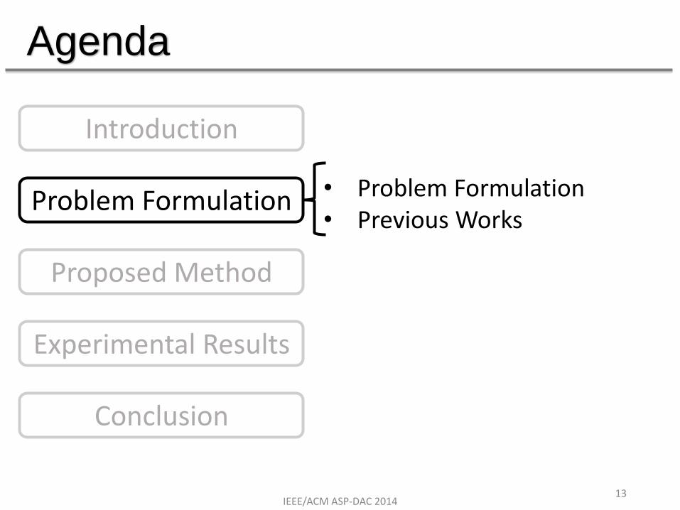
Agenda
Introduction
Problem Formulation
Proposed Method
Experimental Results
Conclusion
IEEE/ACM ASP-DAC 2014 2

Agenda
Problem Formulation
Proposed Method
Experimental Results
Conclusion
• Digital Microfluidic Biochips • Sample Preparation • Illustrative Example
Introduction
IEEE/ACM ASP-DAC 2014 3

Digital Microfluidic Biochips (DMFBs)
• Architecture of a DMFB: • 2D microfluidic array: Basic cells for biological reactions
• Droplets: Biological samples (picoliter unit)
• I/O ports, peripheral devices (detector, …)
• Applications: Immunoassay, DNA sequencing, protein crystallization, etc.
Dispensing port
Electrodes
Droplet
Optical
detector
IEEE/ACM ASP-DAC 2014 4

Sample Preparation (1/4)
• To produce droplets of the required concentrations
• A crucial preprocessing step in every application • 90% of the cost and 95% of the analysis time
Sample preparation
Sample droplets (c = 100%)
Buffer droplets (c = 0%)
Waste droplets
75
%
target droplet
Expensive cost !!!
$$$
single-target
Processing time, reliability !!!
IEEE/ACM ASP-DAC 2014 5

Sample Preparation (2/4)
• To produce droplets of the required concentrations
• A crucial preprocessing step in every application • 90% of the cost and 95% of the analysis time
Sample preparation
Sample droplets (c = 100%)
Buffer droplets (c = 0%)
Waste droplets
75
%
50
% 75
%
80
%
75
%
20
%
multi-target … …
IEEE/ACM ASP-DAC 2014 6
Expensive cost !!!
$$$
Processing time, reliability !!!
Optimization needed !!!

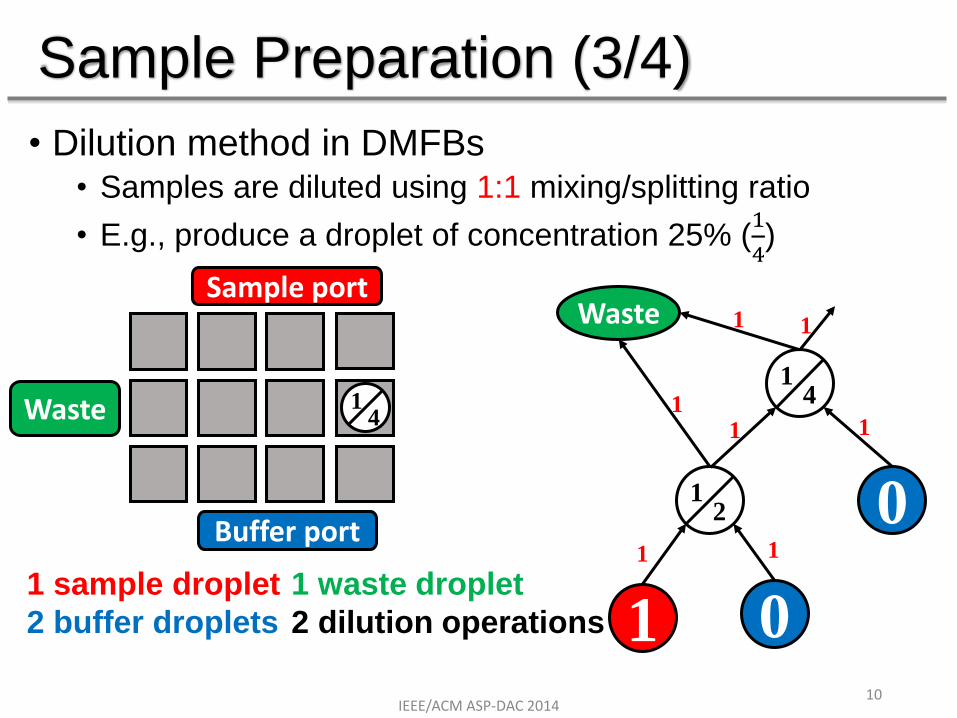
Sample Preparation (3/4)
• Dilution method in DMFBs • Samples are diluted using 1:1 mixing/splitting ratio
• E.g., produce a droplet of concentration 25% (1
4)
Sample port
Buffer port
1
0 1
2
1 2 Waste
IEEE/ACM ASP-DAC 2014 7
1 1
1 0

Sample Preparation (3/4)
• Dilution method in DMFBs • Samples are diluted using 1:1 mixing/splitting ratio
• E.g., produce a droplet of concentration 25% (1
4)
1 2
1 2
1 2
1 2 1
1
IEEE/ACM ASP-DAC 2014 8
Sample port
Buffer port
1 sample droplet
1 buffer droplet
1 waste droplet
1 dilution operation
1 1
1 0
Waste
Waste

1 sample droplet
2 buffer droplets
Sample Preparation (3/4)
• Dilution method in DMFBs • Samples are diluted using 1:1 mixing/splitting ratio
• E.g., produce a droplet of concentration 25% (1
4)
1 2
1 4
1 1 1 1
2 1
4
IEEE/ACM ASP-DAC 2014 9
0
Sample port
Buffer port 0 1 sample droplet
1 buffer droplet
1 waste droplet
1 dilution operation
1 1
1 0
Waste
Waste
Sample Preparation (3/4)
• Dilution method in DMFBs • Samples are diluted using 1:1 mixing/splitting ratio
• E.g., produce a droplet of concentration 25% (1
4)
1 2
1 4
1 1
1 1
Waste
1 1 4
1 1
IEEE/ACM ASP-DAC 2014 10
1 0
0
Sample port
Buffer port
1 waste droplet
2 dilution operations
1 sample droplet
2 buffer droplets
Waste

Sample Preparation (4/4)
• In general:
• A concentration value is always expressed by 𝑐𝑖
2𝑑
• d: precision level of concentration
• d is given in each problem
Ci Cj
Ci + Cj
2
n
2n
n
IEEE/ACM ASP-DAC 2014 11

Example: Same targets, but different cost
• d = 6
• Targets: 21
64, 51
64
12
64 0
32 0
16 64
40 0
20 64
42 0
21
1
1 1
1 1
1 1
1 1
1 1
1
1
T
64 0
32 64
48 0
24 0
12 64
38 64
51
1
1 1
1 1
1 1
1 1
1 1
1
1
64 0
32 1 1
16
0
8
0
4
0
12 64
38
51 21
T
1 1
64 1
1 1 1
1 1
1 1 1
1
1 1
1 1 #sample #buffer
7 7
#waste #ops
12 12
#sample #buffer
3 4
#waste #ops
5 8
Agenda
Proposed Method
Experimental Results
Conclusion
• Problem Formulation • Previous Works
Introduction
Problem Formulation
IEEE/ACM ASP-DAC 2014 13

Problem Formulation (1/2)
• Given: • Cost of 1 sample droplet: 𝒄𝒐𝒔𝒕𝒔
• Cost of 1 buffer droplet: 𝒄𝒐𝒔𝒕𝒃
• Precision level of concentration: 𝒅
• A set of 𝑵 target concentrations: 𝑻𝑪 = {𝒄𝟏, 𝒄𝟐, … , 𝒄𝑵}
• A set of the required number of droplets for each target concentration: 𝑺 = 𝒔𝟏, 𝒔𝟐, … , 𝒔𝑵 ; 𝑺𝑹 = 𝒔𝒊
𝑵𝒊=𝟏
• Output: A valid sample preparation process
• Objective: Minimize cost of sample and buffer usage 𝑭 = 𝒖𝒔 × 𝒄𝒐𝒔𝒕𝒔 + 𝒖𝒃 × 𝒄𝒐𝒔𝒕𝒃
𝒖𝒔, 𝒖𝒃: The numbers of used sample/buffer droplets
IEEE/ACM ASP-DAC 2014 14
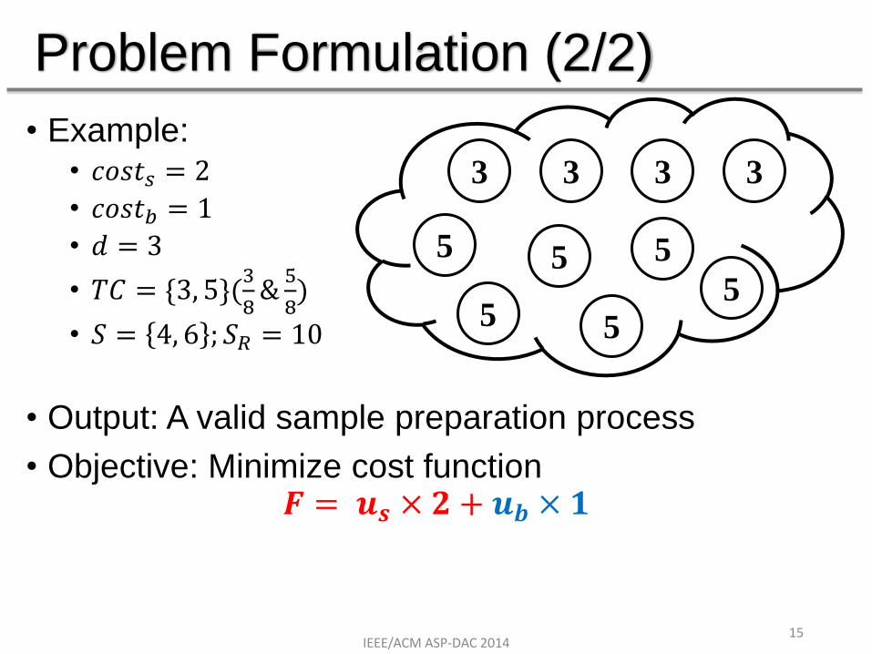
Problem Formulation (2/2)
• Example: • 𝑐𝑜𝑠𝑡𝑠 = 2
• 𝑐𝑜𝑠𝑡𝑏 = 1
• 𝑑 = 3
• 𝑇𝐶 = {3, 5}(3
8&5
8)
• 𝑆 = 4, 6 ; 𝑆𝑅 = 10
• Output: A valid sample preparation process
• Objective: Minimize cost function 𝑭 = 𝒖𝒔 × 𝟐 + 𝒖𝒃 × 𝟏
3 3 3 3
5
5 5
5 5
5
IEEE/ACM ASP-DAC 2014 15

Previous Works
• All the previous works are based on heuristics
• All the previous works focus on only one objective optimization
• Methods that deal with single-target problem (𝑁 = 1) • [W. Thies et al., Natural Computing 2008]: Minimize #operations
• [S. Roy et al., TCAD 2010] : Minimizes #waste droplets
• [S. Roy et al., DATE 2011]: Minimizes #waste droplets
• Methods that deal with multi-target problem (𝑁 > 1) • [Y.-L Hsieh et al., TCAD 2012] : Minimizes #sample droplets
• [J.-D Huang et al., ICCAD 2012] : Minimizes #sample droplets
• [D. Mitra et al., ISVLSI 2012]: Minimizes #operations
Proposed method: Minimize the cost function 𝑭 = 𝒖𝒔 × 𝒄𝒐𝒔𝒕𝒔 + 𝒖𝒃 × 𝒄𝒐𝒔𝒕𝒃
• Optimal solution for multiple-target problem • Flexible to change objective optimization
• By varying the values of 𝒄𝒐𝒔𝒕𝒔 and 𝒄𝒐𝒔𝒕𝒃
• E.g., 𝒄𝒐𝒔𝒕𝒔 = 𝟏 & 𝒄𝒐𝒔𝒕𝒃 = 𝟎⟹ 𝑭 = 𝒖𝒔 (#sample droplets)
IEEE/ACM ASP-DAC 2014 16

Agenda
Proposed Method
Experimental Results
Conclusion
Introduction
Problem Formulation
IEEE/ACM ASP-DAC 2014 17

Overview
Min-cost max-flow (MCMF) network model construction
Input
Integer equal flows problem transformation
ILP solver
Output
IEEE/ACM ASP-DAC 2014 18

MCMF Network Model – Set of Vertices V
• Source, Sink, Waste
• Vertices that represent concentration values • Constructed bottom-up from level 0 to level 𝑑 (e.g., 3)
• Vertices at level 𝑙 represent the set of concentration values that can be generated at this level
Source
Sink Waste Level 3
Level 2
Level 1
Level 0
8 0 3 1 2 4 5 6 7
8 0 2 4 6
8 0 4
8 0
IEEE/ACM ASP-DAC 2014 19

MCMF Network Model – Set of Arcs A
Source
Sink
Waste
Level 3
Level 2
Level 1
Level 0
8 0 3 1 2 4 5 6 7
8 0 2 4 6
8 0 4
8 0
𝑐𝑜𝑠𝑡𝑠 = 2 𝑐𝑜𝑠𝑡𝑏 = 1 𝑑 = 3 𝑇𝐶 = {3, 5} 𝑆 = 4, 6
𝒄𝒐𝒔𝒕 = 𝒄𝒐𝒔𝒕𝒃 = 𝟏 𝒄𝒂𝒑𝒂𝒄𝒊𝒕𝒚 = ∞
𝒄𝒐𝒔𝒕 = 𝒄𝒐𝒔𝒕𝒔 = 𝟐 𝒄𝒂𝒑𝒂𝒄𝒊𝒕𝒚 = ∞
IEEE/ACM ASP-DAC 2014 20
𝒇 𝒃𝒖𝒇𝒇𝒆𝒓 𝒇 𝒔𝒂𝒎𝒑𝒍𝒆
Minimize 𝑭 = 𝒇 𝒃𝒖𝒇𝒇𝒆𝒓 × 𝒄𝒐𝒔𝒕𝒃 + 𝒇 𝒔𝒂𝒎𝒑𝒍𝒆 × 𝒄𝒐𝒔𝒕𝒔

MCMF Network Model – Set of Arcs A
Source
Sink
Waste
Level 3
Level 2
Level 1
Level 0
8 0 3 1 2 4 5 6 7
8 0 2 4 6
8 0 4
8 0
𝑐𝑜𝑠𝑡𝑠 = 2 𝑐𝑜𝑠𝑡𝑏 = 1 𝑑 = 3 𝑇𝐶 = {3, 5} 𝑆 = 4, 6
𝒄𝒐𝒔𝒕 = 𝟎 𝒄𝒂𝒑𝒂𝒄𝒊𝒕𝒚 = ∞
IEEE/ACM ASP-DAC 2014 21

MCMF Network Model – Set of Arcs A
Source
Sink
Waste
Level 3
Level 2
Level 1
Level 0
8 0 3 1 2 4 5 6 7
8 0 2 4 6
8 0 4
8 0
𝑐𝑜𝑠𝑡𝑠 = 2 𝑐𝑜𝑠𝑡𝑏 = 1 𝑑 = 3 𝑇𝐶 = {3, 5} 𝑆 = 4, 6
𝒄𝒐𝒔𝒕 = 𝟎 𝒄𝒂𝒑𝒂𝒄𝒊𝒕𝒚 = ∞
Integer equal flows constraints: 𝒇 𝒂𝒊 = 𝒇 𝒂𝒋 IEEE/ACM ASP-DAC 2014
22

MCMF Network Model – Set of Arcs A
Source
Sink
Waste
Level 3
Level 2
Level 1
Level 0
8 0 3 1 2 4 5 6 7
8 0 2 4 6
8 0 4
8 0
𝑐𝑜𝑠𝑡𝑠 = 2 𝑐𝑜𝑠𝑡𝑏 = 1 𝑑 = 3 𝑇𝐶 = {3, 5} 𝑆 = 4, 6
𝒄𝒐𝒔𝒕 = 𝟎 𝒄𝒂𝒑𝒂𝒄𝒊𝒕𝒚 = 𝒔𝟐 = 𝟔
𝒄𝒐𝒔𝒕 = 𝟎 𝒄𝒂𝒑𝒂𝒄𝒊𝒕𝒚 = 𝒔𝟐 = 𝟒
IEEE/ACM ASP-DAC 2014 23
Target concentration constraints: 𝒇 𝒕𝒂𝒓𝒈𝒆𝒕, 𝑺𝒊𝒏𝒌 = 𝒔𝒊

MCMF Network Model – Set of Arcs A
Source
Sink
Waste
Level 3
Level 2
Level 1
Level 0
8 0 3 1 2 4 5 6 7
8 0 2 4 6
8 0 4
8 0
𝑐𝑜𝑠𝑡𝑠 = 2 𝑐𝑜𝑠𝑡𝑏 = 1 𝑑 = 3 𝑇𝐶 = {3, 5} 𝑆 = 4, 6
𝒄𝒐𝒔𝒕 = 𝟎 𝒄𝒂𝒑𝒂𝒄𝒊𝒕𝒚 = ∞
IEEE/ACM ASP-DAC 2014 24

ILP Model
• Minimize 𝑭 = 𝒇 𝑺𝒐𝒖𝒓𝒄𝒆, 𝒔𝒂𝒎𝒑𝒍𝒆 × 𝒄𝒐𝒔𝒕𝒔 + 𝒇 𝑺𝒐𝒖𝒓𝒄𝒆, 𝒃𝒖𝒇𝒇𝒆𝒓 × 𝒄𝒐𝒔𝒕𝒃
• Subject to • Capacity constraints:
𝑓 𝑣𝑥 , 𝑣𝑦 ≤ 𝑐𝑎𝑝𝑎𝑐𝑖𝑡𝑦 𝑣𝑥, 𝑣𝑦 ∀ 𝑣𝑥, 𝑣𝑦 ∈ 𝐴
• Network-flow conservation:
𝑓 𝑣𝑖 , 𝑣𝑥 =
𝑣𝑖:(𝑣𝑖,𝑣𝑥)∈𝐴
𝑓 𝑣𝑥, 𝑣𝑜𝑣𝑜:(𝑣𝑥,𝑣𝑜)∈𝐴
• Integer equal flow constraints
• Target concentrations constraints
IEEE/ACM ASP-DAC 2014 25

Agenda
Proposed Method
Experimental Results
Conclusion
Introduction
Problem Formulation
IEEE/ACM ASP-DAC 2014 26

Comparative Studies
• Single-target sample preparation problem • [W. Thies et al., Natural Computing’08] [BS]
• [S. Roy et al., IEEE/ACM DATE’11] [DMRW]
• [J.-D Huang et al., IEEE/ACM ICCAD’12] [REMIA]
• Multiple-target sample preparation problem
• [J.-D Huang et al., IEEE/ACM ICCAD’12] [REMIA]
IEEE/ACM ASP-DAC 2014 27

Parameters Settings
• Cost Function 𝑭 = 𝒖𝒔 × 𝒄𝒐𝒔𝒕𝒔 + 𝒖𝒃 × 𝒄𝒐𝒔𝒕𝒃
• Waste droplets: [𝒖𝒔 + 𝒖𝒃 − 𝑺𝑹] • 𝑺𝑹: The total number of target droplets
IEEE/ACM ASP-DAC 2014 28
𝒄𝒐𝒔𝒕𝒔 𝒄𝒐𝒔𝒕𝒃 𝑭 Optimization Objective
1 0 𝒖𝒔 #sample droplets
(𝑜𝑢𝑟𝑠𝑆)
1 1 𝒖𝒔 + 𝒖𝒃 #waste droplets (𝑜𝑢𝑟𝑠𝑊)

Single-Target Sample Preparation
• ILP solver: CPLEX
• 𝑑 = 10
• Target concentrations: 1
1024⇢1023
1024
• Take average values of all 1023 cases
IEEE/ACM ASP-DAC 2014 29
BS DMRW REMIA 𝑜𝑢𝑟𝑠𝑆 𝑜𝑢𝑟𝑠𝑊
# sample droplets 5.00 3.52 2.41 2.22 2.49
# buffer droplets 4.01 3.50 6.09 9.68 2.50
# waste droplets 8.01 6.02 7.50 10.90 3.99
# operations 8.01 12.52 10.13 15.80 9.85

Multiple-Target Sample Preparation • 𝑑 = 8, 9, 10 𝑁 = 10, 20, 50, 100 • For each pair (𝑑, 𝑁), generate 100 random test cases
IEEE/ACM ASP-DAC 2014 30
𝒅 = 𝟗 𝑁 = 10 𝑁 = 100
REMIA 𝑜𝑢𝑟𝑠𝑠 𝑜𝑢𝑟𝑠𝑊 REMIA 𝑜𝑢𝑟𝑠𝑠 𝑜𝑢𝑟𝑠𝑊
# sample droplets 19.59 8.07 8.95 203.98 80.15 80.43
# buffer droplets 31.19 12.67 7.12 277.60 76.44 73.56
# waste droplets 40.78 10.74 6.07 381.58 56.59 53.99
# operations 60.90 43.21 39.69 654.44 276.67 258.84
𝒅 = 𝟏𝟎 𝑁 = 10 𝑁 = 100
REMIA 𝑜𝑢𝑟𝑠𝑠 𝑜𝑢𝑟𝑠𝑊 REMIA 𝑜𝑢𝑟𝑠𝑠 𝑜𝑢𝑟𝑠𝑊
# sample droplets 17.33 11.17 13.96 182.73 101.99 103.41
# buffer droplets 43.35 19.79 11.15 320.25 157.19 97.04
# waste droplets 50.68 20.96 15.11 402.98 159.18 100.45
# operations 89.77 73.12 62.73 720.64 438.36 384.66

Conclusion
• Sample preparation • Pivotal role in every assay, laboratory, and application in
biomedical engineering and life science
• The first optimal sample preparation algorithm is proposed • Based on a minimum-cost maximum-flow model
• Reduce the numbers of sample/buffer/waste droplets & dilution operations significantly
(~60%/70%/85% & 60%, respectively)
IEEE/ACM ASP-DAC 2014 31
Thank you for your attention!!!
Appendix
IEEE/ACM ASP-DAC 2014 32

𝑐𝑜𝑠𝑡 = 0 𝑐𝑎𝑝𝑎𝑐𝑖𝑡𝑦 = ∞
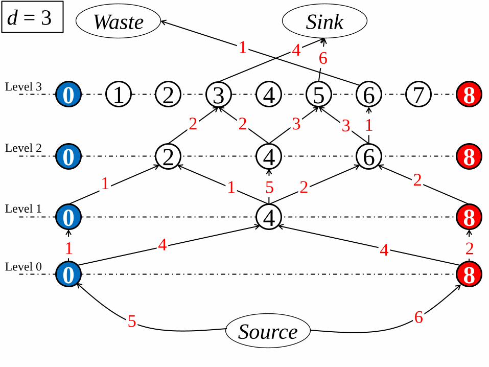
MCMF Network Model – Set of Arcs A
Source
Sink
Waste
Level 3
Level 2
Level 1
Level 0
8 0 3 1 2 4 5 6 7
8 0 2 4 6
8 0 4
8 0
𝑐𝑜𝑠𝑡𝑠 = 2 𝑐𝑜𝑠𝑡𝑏 = 1 𝑑 = 3 𝑇𝐶 = {3, 5} 𝑆 = 4, 6
IEEE/ACM ASP-DAC 2014 33
𝑐𝑜𝑠𝑡 = 𝑐𝑜𝑠𝑡𝑏 = 1 𝑐𝑎𝑝𝑎𝑐𝑖𝑡𝑦 = ∞
𝑐𝑜𝑠𝑡 = 𝑐𝑜𝑠𝑡𝑠 = 2 𝑐𝑎𝑝𝑎𝑐𝑖𝑡𝑦 = ∞
𝑐𝑜𝑠𝑡 = 0 𝑐𝑎𝑝𝑎𝑐𝑖𝑡𝑦 = ∞
𝑐𝑜𝑠𝑡 = 0 𝑐𝑎𝑝𝑎𝑐𝑖𝑡𝑦 = 𝑠2 = 6
𝑐𝑜𝑠𝑡 = 0 𝑐𝑎𝑝𝑎𝑐𝑖𝑡𝑦 = ∞
8 0 3 1 2 4 5 6 7
8 0 2 4 6
8 0 4
8 0
Level 3
Level 2
Level 1
Level 0
Source
Waste d = 3
2
5 6
4 1 4 2
2 5 1 1
2 2 3 3
6
1
Sink
4 1
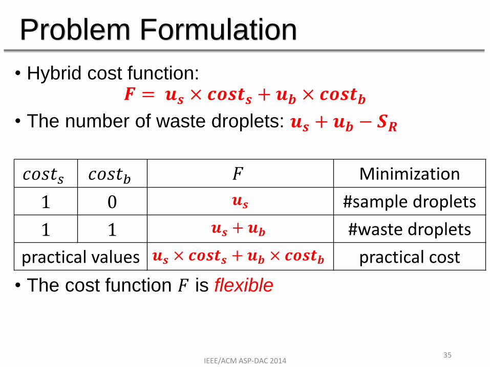
Problem Formulation
• Hybrid cost function: 𝑭 = 𝒖𝒔 × 𝒄𝒐𝒔𝒕𝒔 + 𝒖𝒃 × 𝒄𝒐𝒔𝒕𝒃
• The number of waste droplets: 𝒖𝒔 + 𝒖𝒃 − 𝑺𝑹
• The cost function 𝐹 is flexible
𝑐𝑜𝑠𝑡𝑠 𝑐𝑜𝑠𝑡𝑏 𝐹 Minimization
1 0 𝒖𝒔 #sample droplets
1 1 𝒖𝒔 + 𝒖𝒃 #waste droplets
practical values 𝒖𝒔 × 𝒄𝒐𝒔𝒕𝒔 + 𝒖𝒃 × 𝒄𝒐𝒔𝒕𝒃 practical cost
IEEE/ACM ASP-DAC 2014 35
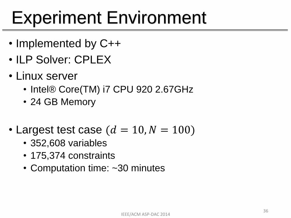
Experiment Environment
• Implemented by C++
• ILP Solver: CPLEX
• Linux server • Intel® Core(TM) i7 CPU 920 2.67GHz
• 24 GB Memory
• Largest test case (𝑑 = 10, 𝑁 = 100) • 352,608 variables
• 175,374 constraints
• Computation time: ~30 minutes
IEEE/ACM ASP-DAC 2014 36
Digital Microfluidic Biochips (DMFBs) (2/2)
• Advantages: • High portability
• High throughput
• Low sample volume consumption
• Less human intervention errors
• Applications: immunoassay, DNA sequencing, protein crystallization, etc.
IEEE/ACM ASP-DAC 2014 37