A molecular dynamics study on universal properties of polymer chains in differentsolvent qualities. Part I. A review of linear chain propertiesMartin Oliver Steinhauser

Citation: The Journal of Chemical Physics 122, 094901 (2005); doi: 10.1063/1.1846651 View online: http://dx.doi.org/10.1063/1.1846651 View Table of Contents: http://scitation.aip.org/content/aip/journal/jcp/122/9?ver=pdfcov Published by the AIP Publishing Articles you may be interested in Molecular dynamics simulation study of solvent effects on conformation and dynamics of polyethylene oxide andpolypropylene oxide chains in water and in common organic solvents J. Chem. Phys. 136, 124901 (2012); 10.1063/1.3694736 Brownian dynamics simulations of single polymer chains with and without self-entanglements in theta and goodsolvents under imposed flow fields J. Rheol. 54, 1061 (2010); 10.1122/1.3473925 Polymer brushes in solvents of variable quality: Molecular dynamics simulations using explicit solvent J. Chem. Phys. 127, 084905 (2007); 10.1063/1.2768525 Kinetics of chain collapse in dilute polymer solutions: Molecular weight and solvent dependences J. Chem. Phys. 126, 134901 (2007); 10.1063/1.2715596 Conformations of attractive, repulsive, and amphiphilic polymer chains in a simple supercritical solvent:Molecular simulation study J. Chem. Phys. 119, 4026 (2003); 10.1063/1.1591722

This article is copyrighted as indicated in the article. Reuse of AIP content is subject to the terms at: http://scitation.aip.org/termsconditions. Downloaded to IP:

92.245.150.83 On: Mon, 31 Mar 2014 10:05:51

A molecular dynamics study on universal properties of polymer chainsin different solvent qualities. Part I. A review of linear chain properties

Martin Oliver Steinhausera!

Fraunhofer Ernst-Mach-Institute for High-Speed Dynamics, 79104 Freiburg, Germany

sReceived 13 May 2004; accepted 16 November 2004; published online 24 February 2005d

This paper investigates the conformational and scaling properties of long linear polymer chains.These investigations are done with the aid of Monte CarlosMCd and molecular dynamicssMDdsimulations. Chain lengths that comprise several orders of magnitude to reduce errors of finite sizescaling, including the effect of solvent quality, ranging from the athermal limit over theu-transitionto the collapsed state of chains are investigated. Also the effect of polydispersity on linear chains isincluded which is an important issue in the real fabrication of polymers. A detailed account of thehybrid MD and MC simulation model and the exploited numerical methods is given. Many resultsof chain properties in the extrapolated limit of infinite chain lengths are documented and universalproperties of the chains within their universality class are given. An example of the differencebetween scaling exponents observed in actual solvents and those observed in the extremes of “goodsolvents” and “u-solvents” in simulations is provided by comparing simulation results withexperimental data on low density polyethylene. This paper is concluded with an outlook on theextension of this study to branched chain systems of many different branching types. ©2005American Institute of Physics. fDOI: 10.1063/1.1846651g

I. INTRODUCTION

Due to their large masses, polymers possess an enor-mous variety of conformations with different sizes andshapes. The study of these conformations on a microscopicscale is a key to understanding the different properties ofmacromolecular systems. Hence, for the theoretical descrip-tion of such systems one has to fall back upon the resourcesof statistical mechanics. By this turning away from the at-tempt to formulate theories that are based directly on theelectronic and chemical structure, one can introduce simpli-fied models which provide insight into macroscopic proper-ties of polymers that depend universally on only a few pa-rameters such as the chain length or interaction strength.Usually, experiments with polymers are done in solvents ofvariable qualities which give rise to solvent–polymer inter-actions. These interactions can be characterized by a Floryparameterx sRef. 1d which depends on temperatureT. Thephase diagram of experimental solvent–polymer systems isgiven in terms of concentrationc and temperatureT. Whenone introduces an effective length per monomer,a, and thevolume fraction of monomers,F=ca3, the phase diagramassumes a universal structure. This universal behavior ofpolymers along with the statistical nature of polymer systemsis the reason why computer simulations are useful for theinvestigation of structural properties.

One great advantage with computer simulations is thepossibility to study model systems of polymers without thetypical errors and restrictions that one has to deal with whenperforming experiments. However, simulations only testmodel-systems of reality and their outcome has to be vali-

dated against both, theory and experiments, which is usuallydone by comparing dimensionless parameters.

In this work, a continuous simulation model is devel-oped which allows for the investigation of universal proper-ties of polymer chains, expressed in dimensionless param-eters, such as size expansion factorsa2 or r which aredefined as

a2 =kRg

2lkRg

2l0

, s1d

r = kRg2l1/2/kRh

−1l−1, s2d

whereRg is the radius of gyration,Rh is the hydrodynamicradius, and the subscript 0 indicatesu-conditions.Rh is ex-perimentally determined by dynamic light scattering2 and de-scribes the equivalent radius of a polymer chain in a flowfield. In computer simulations it can be measured as a staticquantity and is defined as3

K 1

RhL =

1

N2oiÞ jK 1

ur i − r juL , s3d

whereN is the total number of monomers andr i is the posi-tion vector to theith monomer. This simulation study is incontrast to very many simulation studies of such chain prop-erties which were only done on various lattices and withconsiderably shorter chain lengths. Also, the universal scal-ing properties of polymers are not being taken account of inexperimental literature on scaling properties of polymers andalso in simulation studies the obtained chain properties areusually not extrapolated to the limit of infinitely long chainswhich gives rise to large corrections to scalingsfinite sizescalingd. The detailed nature of these finite size corrections to

adElectronic mail: Martin.Steinhauser@emi.fraunhofer.deURL: www.emi.fraunhofer.de

THE JOURNAL OF CHEMICAL PHYSICS122, 094901s2005d

0021-9606/2005/122~9!/094901/13/$22.50 © 2005 American Institute of Physics122, 094901-1

This article is copyrighted as indicated in the article. Reuse of AIP content is subject to the terms at: http://scitation.aip.org/termsconditions. Downloaded to IP:

92.245.150.83 On: Mon, 31 Mar 2014 10:05:51

scaling was studied with our very precise data of long linearchains and was published elsewhere.4 The results of thiswork were obtained with a newly developed state-of-the-artprogram package3MD “Triple MD” and improve the exact-ness of data concerning polymer structure and scaling prop-erties by at least one order of magnitude compared to previ-ous studies.

First, a detailed account of the properties of the simula-tion model is given which includes effects of different sol-vent qualities as a crucial point for the comparison of simu-lation results with experimental data.

II. THE POLYMER MODEL

In order to study many properties of polymer chains it issufficient to model just a few key properties of polymer sys-tems such as the connectivity of monomersstopological con-straintsd, the noncrossability of different chains and the flex-ibility of the monomer segments. One of the mainadvantages of this approach is that one has to deal with onlya few simulation parameters which in turn allows one tochoose the model that is most convenient in terms of com-putational expenditure. An incorporation of full chemical de-tails of very long polymer chains would prove intractablenumerically even with present-day computer equipment. Inorder to gain important universal properties of long chains ingeneral, the chemical details are not needed.

In the simulations presented here a bead-spring-model ofchains is used which has been used in many variations.5–8

Coarse-graining is achieved by replacing a subchain of a realpolymer by a soft bead and a spring with a suitable forceelongation law. Friction and mass of the subchains arelumped into the beads which exhibit an excluded volume ofa Lennard-Jones-type.9

For simulation purposes reduced units for the energye=kBT=1, s=1 are used and time is measured in units oft=Îms2/e. For reasons of efficiency, a potential that is to beused in simulations should be short-ranged in order to keepforce calculations at a minimum. As in this study long rangeforces such as Coulomb forces are not being taken into ac-count, the intermolecular potential is cut off at its minimumrmin and shifted to positive values such that it becomespurely repulsive and smoothly approaches zero. The expres-sion for this Weeks–Chandler–Andersen potential10 is

VWCAsrd = 4eHSs

rD12

− Ss

rD6J + e, s4d

0 , r ø rmin = 21/6s.

In order to be able to simulate systems at varying solventqualities an attractive term is smoothly added to the potentialin Eq. s4d,

Vcossrd = f 12 · cossar2 + bd + 0.5ge, rmin , r , rcut. s5d

The parametersa andb are obtained by demanding thatthe cosine part fits smoothly to the Lennard-Jones potentialat the minimum value ofrmin and that the combined potentialis zero at the chosen cutoffrcut=1.5 s. Demanding this, oneyields the following equations:

a = 3.1730728678, s6d

b = − 0.856228645. s7d

This potential has been used successfully for the simu-lation of shear in polymer binary mixtures.11

The form of the intermolecular potential between mono-mer beads reads

Vintersrd = 5VWCAsrd − le 0 , r , 21/6s

lVcossrd 21/6s ø r , rcut

0 else,6 s8d

where l is a newly introduced dimensionless parameterwhich determines the depth of the used potential. Instead ofvarying the solvent quality by changing temperatureT di-rectly, allowing for a phase transition of the system, the verysame effect is achieved in our model by varying the interac-tion parameterl between particles.l=0.0 corresponds to theathermal casesideal solventd, and values ofl.0 correspondto decreasing solvent quality. Therefore, in all simulations,the temperature parameterT can be kept at a constant valuekBT=1.0 e and only the parameterl is varied.

Since chemical bonds have a fixed length, real polymersare rather inextensible. This can be modeled by a nonlinearspring law which keeps the stretching of the springs smalleven for large forces. Rather common in simulations is thephenomenological FENEsfinitely extendable nonlinear elas-ticd potential as an intramolecular potential which reads

Vintrasrd = 5−1

2kR0

2 lnS1 −r2

R02D r , R0

0 else.6 s9d

The values for the parameters are chosen asR0=1.5 sandk=30 e /s2 which have proven to be useful in practice.12

The total potential finally is given by the following equa-tion:

Vtotalsrd = Vintersrd + Vintrasrd. s10d

The density r=N/V of the systems is chosen asr=0.85s−3 throughout all simulations. This is the density ofliquid polymer systems for which the potential parametershave been optimized. The code3MD can be used for simu-lations of polymers in a melt, as well as for the simulation ofsingle chain systems by switching off the interchain interac-tion. The latter allows for simulating large ensembles of iso-lated chains and, as a result, improves statistics considerably.

A. Integration scheme: Molecular dynamics

In the molecular dynamics part of the simulation a cubicsimulation box with periodic boundary conditions is used,avoiding surface effects and only considering bulk-propertiesof particles. The implementation of periodicity was done in avery efficient way by making use of the concept ofghost-particles.7 Many different integration schemes for dif-ferent ensembles have been proposed.6,13–17The influence ofthe surrounding of the polymers is taken into account bycoupling the system to a heat bath. This can be done inseveral ways. One method was proposed by Nosé, which

094901-2 Martin Oliver Steinhauser J. Chem. Phys. 122, 094901 ~2005!

This article is copyrighted as indicated in the article. Reuse of AIP content is subject to the terms at: http://scitation.aip.org/termsconditions. Downloaded to IP:

92.245.150.83 On: Mon, 31 Mar 2014 10:05:51

couples the system to a heat bath by enlarging the degrees offreedom of phase space18,19 and a modified version was in-troduced in Ref. 20. In this work a canonical NVT-ensembleis integrated and the coupling of the system to a heat bath isdone by splitting the forceFstd into a slowly changing fric-tion forceFg of Stoke’s type and a fast fluctuating stochasticforce FS which leads to the integration of a Langevin differ-ential equation:

r std = − gvstd + fstd + Gstd, s11d

with −gvstd=Fg /m, fstd=F /m, Gstd=FS/m, m being the par-ticle mass andg being the friction coefficient. The propertiesof the Langevin-force are given by the fluctuation-dissipationtheorem.21 We integrate Eq.s11d with the following scheme:

r ist + Dtd = r istd + DtvistdF1 − gDt

2miG +

Dt2

2miT istd, s12d

vist + Dtd =

vistdF1 − gDt

2miG +

Dt

2mifT istd + T ist + Dtdg

1 + gDt

2mi

,

s13d

with total force

T i = Fi + Gi . s14d

The use of a stochastic term in the equations of motionexplicitly destroys time-reversibility and avoids ergodicityproblems of microcanonical simulation schemes. It allowsfor a larger time stepDtù0.005t in the simulation as thecoupling to a heat bath generally makes a simulation morestable. In this work, for all simulations a time step ofDt=0.01t and a friction coefficient ofg=1.0 were used. Onthe other hand, with stochastic dynamics simulations, it isnot possible to investigate properties depending on longrange correlations such as hydrodynamic interactions.

B. Integration scheme: Monte Carlo

Chain polymers were among the first objects simulatedon electronic computers and they still present a challenge,because of the particular structure of this problem which in-volves the relaxation of the chain on different length scales.This problem of multi scale relaxation is tackled by exploit-ing molecular dynamics methods for the relaxation of smalllength scales and use another very efficient algorithm forrelaxing the considered systems on largesglobald lengthscales.

Straightforward algorithms such as simple sampling areoften inefficient and a whole host of methods has been pro-posed, all with certain merits and disadvantages.8,22–24 Onevery efficient method to obtain equilibrium samples on asimple-cubic lattice was proposed in Refs. 25,26. Thismethod combines the Rosenbluth–Rosenbluth method withrecursive enrichment and is called PERMsPruned-EnrichedRosenbluth Methodd.

Today it seems that the pivot algorithm, which was pro-posed by Lal in 1969sRef. 27d is the most popular one in

order to gain equilibrium samples of single chains in thecontinuum or on a lattice. Stellman applied this algorithm tooff-lattice simulations of a hard-sphere polymer model.28

Pivoting a chain in its configuration space proved to bemost efficient for relatively open, dilute systems such as iso-lated linear chains,29,30 but also for self-avoiding star-branched polymers,31,32 where the segment density near thebranching point is relatively large in comparison with thelinear chain. The algorithm proved very efficient for both,lattice and continuum models.23 However, it becomes ineffi-cient in dense or constrained systems where most of the glo-bal movesswhich make it fast in dilute systemsd are rejecteddue to overlaps with other chains, see Fig. 1.

An illustration of a pivot move with a linear chain isgiven in Fig. 2. A configurational change of the chain isachieved by rotating one part of the chain around a randomlyselected bond. This new configuration undergoes a Metropo-lis algorithm according to which the new configuration iseither accepted or rejected. Thus, the pivot algorithm fitsperfectly into the scheme of the Metropolis algorithm withthe only difference being that a whole part of the chain ismoved in phase space as opposed to a single particle in theoriginal scheme.

The pivot algorithm was applied in all presented simu-lations of single chains in this work: After having chosen atrandom a particlek with coordinater 0 of the chain as spin

FIG. 1. Acceptance rate of pivot moves for linear chains as a function of themolecular weightN and the interaction strengthl during a hybrid simula-tion in which pivot moves were used alternately with MD simulation steps.Only for very long chains the pivot algorithm does become inefficient.

FIG. 2. Illustration of a pivot move. The grey shaded original part of thechain is rotated about a randomly chosen normal vectorn.

094901-3 Universal properties of polymer chains in different solvents J. Chem. Phys. 122, 094901 ~2005!

This article is copyrighted as indicated in the article. Reuse of AIP content is subject to the terms at: http://scitation.aip.org/termsconditions. Downloaded to IP:

92.245.150.83 On: Mon, 31 Mar 2014 10:05:51

center, all the rest of the chainsto say, all particles withindices larger thankd is rotated about this particlek. Toachieve this, a random rotation matrixR is calculated foreach pivot move such that for the new positionsr 8 of therotated part the following equation holds:

r 8 = r 0 + Rn,asr − r 0d. s15d

The random rotation matrixR is given by a normal vec-tor n=nsq ,wd in spherical coordinates and a rotation anglea. R applied to a vectorr yields

Rn,ar = r cosa + snr ds1 − cosadn + sn 3 r dsina, s16d

wherea ,w and cosq are chosen equally distributed from theinterval f0,2pg and f−1,1g, respectively.

The global moves of the pivot algorithm allow for a fastrelaxation of a chain on large length scales. To speed up therelaxation on short length scales, too, MD simulation stepswere also performed at certain time intervals. In Fig. 1 theefficiency of the pivot moves when applying this hybrid-algorithm is shown for different chain lengths and differentvalues of the interaction parameterl of Eq. s8d. The accep-tance rate is well above 50% for smaller systems and alsounderu-conditions, in the vicinity ofl<0.65, one still has ahigh enough acceptance of global moves to relax the chainsvery efficiently.

III. RESULTS

A. Different solvent qualities

In this section the influence of temperature, respectivelysolvent quality on dilute solution properties of flexible linearchains according to the implemented polymer chain model ispresented. In this analysis it was gone beyond most previousinvestigators who mostly concentrated on simulations ofrather short chains in the vicinity of theu-point. In this study,the whole temperature range from an ideally good solvent toa very bad solvent is covered with chain lengths of up toN=2000. Simulations of chain lengths ofN=5000 were alsodone for the athermal case and at theu-point.

The collapse transition of chains was subject of muchtheoretical work. The type of transition in the limit of infinitechain length was discussed in Ref. 33. It was pointed out byde Gennes1 that the u-point is a tricritical point and thatmean field theory can be applied, except for logarithmic cor-rections. An overview of early studies is given in Ref. 34.Numerous simulations have been performed, mainly focus-ing on the use of various MC-methods on lattices.35–39

In experiments, it is difficult to obtain complete and con-clusive results in the study of the collapse transition ofchains, because one is restricted to solutions of extremelydilute polymer concentrations.40

At the u-temperature the chains behave askRg2l~ kRe

2l~ sN−1d2nu with nu=0.5 besides logarithmic corrections ind=3. With R denoting either the radius of gyrationRg or theend-to-end distanceRe, one expects that a plot ofkR2l / sN−1d versusT for different values ofN shows a commonintersection point atT=Tu where the curvature changes: forT.Tu the largerN, the larger the ratiokR2l / sN−1d has to be,while for T,Tu the largerN, the smaller the ratiokR2l / sN

−1d has to be. In this work, instead of varying temperature,different solvent qualities were obtained by tuning the inter-action parameterl.

The corresponding transition curves are displayed inFigs. 3 and 4 for the radius of gyration which show a clearintersection point at roughlyl=lu<0.65. Also it can beseen that the transition becomes sharper with increasingchain lengthN in agreement with other investigators.41,42Theshape of the curves is in agreement to those obtained bynumerical studies and experiments.37,43

The different curves do not intersect exactly at onesingle point, but there is an extended region in which thechains behave in a Gaussian manner. The size of this regionis ~N−1/2. There is a very slight drift of the intersection pointtowards a smaller value ofl with increasing chain length.Therefore, to obtain a more precise estimate of theu-temperature in the limit ofsN→`d, one has to chose adifferent graph that allows an appropriate extrapolation. Ifone draws straight horizontal lines in Fig. 3, the intersectionpoints of these lines with the curves are points at which the

FIG. 3. Plot of kRg2l / sN−1d vs interaction parameterl for linear chains.

The points represent the simulated data and the dotted lines are guides to theeye.n=nu=0.5.

FIG. 4. Plot ofl vs N−1/2 for different values of the scaling function. Dataare based on the radius of gyration of linear chains presented in Fig. 3. Thestraight lines are obtained by linear regression allowing for an error estimateof the determination of theu-point.

094901-4 Martin Oliver Steinhauser J. Chem. Phys. 122, 094901 ~2005!

This article is copyrighted as indicated in the article. Reuse of AIP content is subject to the terms at: http://scitation.aip.org/termsconditions. Downloaded to IP:

92.245.150.83 On: Mon, 31 Mar 2014 10:05:51

universal scaling function is constant.1 Plotting different in-tersection points overN−1/2 should therefore yield differentstraight lines that intersect each other exactly atT=Tu andl=lu, respectively. This extrapolation tosN→`d is dis-played in Fig. 4. The different lines do not intersect atN−1/2=0 which is due to the finiteness of the chains. As aresult of these plots one yields

lu = 0.65 ± 0.02. s17d

In principle, the hydrodynamic radiusRh should followthe same scaling laws asRg andRe. It turns out however, thatRh is not suited for a similar analysis of theu-point, becauseof huge corrections to scaling. A detailed discussion andanalysis of these finite size effects based on simulation datahas been published elsewhere.4

Next, a study of the chain length dependence of the coilsize at several fixed temperatures, respectively solvent quali-ties is presented, in order to determine the different scalingexponents directly from the simulation data.

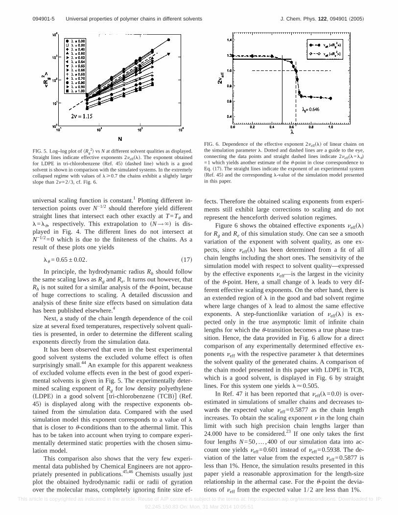
It has been observed that even in the best experimentalgood solvent systems the excluded volume effect is oftensurprisingly small.44 An example for this apparent weaknessof excluded volume effects even in the best of good experi-mental solvents is given in Fig. 5. The experimentally deter-mined scaling exponent ofRg for low density polyethylenesLDPEd in a good solventftri-chlorobenzenesTCBdg sRef.45d is displayed along with the respective exponents ob-tained from the simulation data. Compared with the usedsimulation model this exponent corresponds to a value oflthat is closer tou-conditions than to the athermal limit. Thishas to be taken into account when trying to compare experi-mentally determined static properties with the chosen simu-lation model.

This comparison also shows that the very few experi-mental data published by Chemical Engineers are not appro-priately presented in publications.45,46 Chemists usually justplot the obtained hydrodynamic radii or radii of gyrationover the molecular mass, completely ignoring finite size ef-

fects. Therefore the obtained scaling exponents from experi-ments still exhibit large corrections to scaling and do notrepresent the henceforth derived solution regimes.

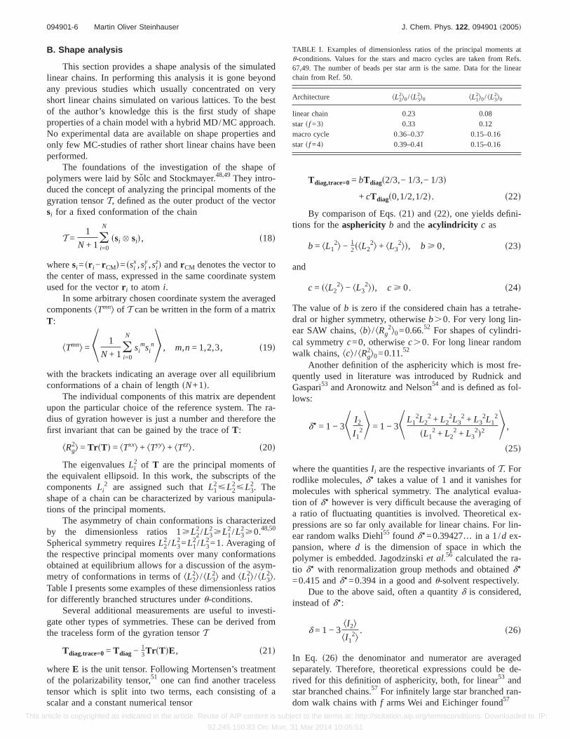
Figure 6 shows the obtained effective exponentsneffsldfor Rg andRe of this simulation study. One can see a smoothvariation of the exponent with solvent quality, as one ex-pects, sinceneffsld has been determined from a fit of allchain lengths including the short ones. The sensitivity of thesimulation model with respect to solvent quality—expressedby the effective exponentsneff—is the largest in the vicinityof the u-point. Here, a small change ofl leads to very dif-ferent effective scaling exponents. On the other hand, there isan extended region ofl in the good and bad solvent regimewhere large changes ofl lead to almost the same effectiveexponents. A step-functionlike variation ofneffsld is ex-pected only in the true asymptotic limit of infinite chainlengths for which theu-transition becomes a true phase tran-sition. Hence, the data provided in Fig. 6 allow for a directcomparison of any experimentally determined effective ex-ponentsneff with the respective parameterl that determinesthe solvent quality of the generated chains. A comparison ofthe chain model presented in this paper with LDPE in TCB,which is a good solvent, is displayed in Fig. 6 by straightlines. For this system one yieldsl<0.505.

In Ref. 47 it has been reported thatneffsl=0.0d is over-estimated in simulations of smaller chains and decreases to-wards the expected valueneff=0.5877 as the chain lengthincreases. To obtain the scaling exponentn in the long chainlimit with such high precision chain lengths larger than24.000 have to be considered.23 If one only takes the firstfour lengthsN=50,… ,400 of our simulation data into ac-count one yieldsneff=0.601 instead ofneff=0.5938. The de-viation of the latter value from the expectedneff=0.5877 isless than 1%. Hence, the simulation results presented in thispaper yield a reasonable approximation for the length-sizerelationship in the athermal case. For theu-point the devia-tions of neff from the expected value 1/2 are less than 1%.

FIG. 5. Log–log plot ofkRg2l vs N at different solvent qualities as displayed.

Straight lines indicate effective exponents 2neffsld. The exponent obtainedfor LDPE in tri-chlorobenzenesRef. 45d sdashed lined which is a goodsolvent is shown in comparison with the simulated systems. In the extremelycollapsed regime with values oflù0.7 the chains exhibit a slightly largerslope than 2n=2/3, cf. Fig. 6.

FIG. 6. Dependence of the effective exponent 2neffsld of linear chains onthe simulation parameterl. Dotted and dashed lines are a guide to the eye,connecting the data points and straight dashed lines indicate 2neffsl=lud=1 which yields another estimate of theu-point in close correspondence toEq. s17d. The straight lines indicate the exponent of an experimental systemsRef. 45d and the correspondingl-value of the simulation model presentedin this paper.

094901-5 Universal properties of polymer chains in different solvents J. Chem. Phys. 122, 094901 ~2005!

This article is copyrighted as indicated in the article. Reuse of AIP content is subject to the terms at: http://scitation.aip.org/termsconditions. Downloaded to IP:

92.245.150.83 On: Mon, 31 Mar 2014 10:05:51

B. Shape analysis

This section provides a shape analysis of the simulatedlinear chains. In performing this analysis it is gone beyondany previous studies which usually concentrated on veryshort linear chains simulated on various lattices. To the bestof the author’s knowledge this is the first study of shapeproperties of a chain model with a hybrid MD/MC approach.No experimental data are available on shape properties andonly few MC-studies of rather short linear chains have beenperformed.

The foundations of the investigation of the shape ofpolymers were laid by Soˇlc and Stockmayer.48,49They intro-duced the concept of analyzing the principal moments of thegyration tensorT, defined as the outer product of the vectorsi for a fixed conformation of the chain

T =1

N + 1oi=0

N

ssi ^ sid, s18d

wheresi =sr i −r CMd=ssix,si

y,sizd andr CM denotes the vector to

the center of mass, expressed in the same coordinate systemused for the vectorr i to atomi.

In some arbitrary chosen coordinate system the averagedcomponentskTmnl of T can be written in the form of a matrixT:

kTmnl =K 1

N + 1oi=0

N

simsi

nL , m,n = 1,2,3, s19d

with the brackets indicating an average over all equilibriumconformations of a chain of lengthsN+1d.

The individual components of this matrix are dependentupon the particular choice of the reference system. The ra-dius of gyration however is just a number and therefore thefirst invariant that can be gained by the trace ofT:

kRg2l = Tr sTd = kTxxl + kTyyl + kTzzl. s20d

The eigenvaluesLi2 of T are the principal moments of

the equivalent ellipsoid. In this work, the subscripts of thecomponentsLi

2 are assigned such thatL12øL2

2øL32. The

shape of a chain can be characterized by various manipula-tions of the principal moments.

The asymmetry of chain conformations is characterizedby the dimensionless ratios 1ùL2

2/L32ùL1

2/L32ù0.48,50

Spherical symmetry requiresL22/L3

2=L12/L3

2=1. Averaging ofthe respective principal moments over many conformationsobtained at equilibrium allows for a discussion of the asym-metry of conformations in terms ofkL2

2l / kL32l and kL1

2l / kL32l.

Table I presents some examples of these dimensionless ratiosfor differently branched structures underu-conditions.

Several additional measurements are useful to investi-gate other types of symmetries. These can be derived fromthe traceless form of the gyration tensorT

Tdiag,trace=0 = Tdiag − 13Tr sTdE, s21d

whereE is the unit tensor. Following Mortensen’s treatmentof the polarizability tensor,51 one can find another tracelesstensor which is split into two terms, each consisting of ascalar and a constant numerical tensor

Tdiag,trace=0= bTdiags2/3,− 1/3,− 1/3d

+ cTdiags0,1/2,1/2d. s22d

By comparison of Eqs.s21d and s22d, one yields defini-tions for theasphericity b and theacylindricity c as

b = kL12l − 1

2skL22l + kL3

2ld, b ù 0, s23d

and

c = skL22l − kL3

2ld, c ù 0. s24d

The value ofb is zero if the considered chain has a tetrahe-dral or higher symmetry, otherwiseb.0. For very long lin-ear SAW chains,kbl / kRg

2l0=0.66.52 For shapes of cylindri-cal symmetryc=0, otherwisec.0. For long linear randomwalk chains,kcl / kRg

2l0=0.11.52

Another definition of the asphericity which is most fre-quently used in literature was introduced by Rudnick andGaspari53 and Aronowitz and Nelson54 and is defined as fol-lows:

d! = 1 − 3K I2

I12L = 1 − 3KL1

2L22 + L2

2L32 + L3

2L12

sL12 + L2

2 + L32d2 L ,

s25d

where the quantitiesI i are the respective invariants ofT. Forrodlike molecules,d! takes a value of 1 and it vanishes formolecules with spherical symmetry. The analytical evalua-tion of d! however is very difficult because the averaging ofa ratio of fluctuating quantities is involved. Theoretical ex-pressions are so far only available for linear chains. For lin-ear random walks Diehl55 found d!=0.39427… in a 1/d ex-pansion, whered is the dimension of space in which thepolymer is embedded. Jagodzinskiet al.56 calculated the ra-tio d! with renormalization group methods and obtainedd!

=0.415 andd!=0.394 in a good andu-solvent respectively.Due to the above said, often a quantityd is considered,

instead ofd!:

d = 1 − 3kI2lkI1

2l. s26d

In Eq. s26d the denominator and numerator are averagedseparately. Therefore, theoretical expressions could be de-rived for this definition of asphericity, both, for linear53 andstar branched chains.57 For infinitely large star branched ran-dom walk chains withf arms Wei and Eichinger found57

TABLE I. Examples of dimensionless ratios of the principal moments atu-conditions. Values for the stars and macro cycles are taken from Refs.67,49. The number of beads per star arm is the same. Data for the linearchain from Ref. 50.

Architecture kL22l0/ kL3

2l0 kL12l0/ kL3

2l0

linear chain 0.23 0.08star sf =3d 0.33 0.12macro cycle 0.36–0.37 0.15–0.16star sf =4d 0.39–0.41 0.15–0.16

094901-6 Martin Oliver Steinhauser J. Chem. Phys. 122, 094901 ~2005!

This article is copyrighted as indicated in the article. Reuse of AIP content is subject to the terms at: http://scitation.aip.org/termsconditions. Downloaded to IP:

92.245.150.83 On: Mon, 31 Mar 2014 10:05:51

d =150f−1 − 140f−2

135 − 120f−1 + 4f−2 , s27d

which is a generalization of the treatment by Rudnik andGaspari53 and reduces tod<0.5263 with f =1 for linearchains. By use of an«-expansion54 a slightly higher value ofd=0.534 has been found for self-avoiding random walks.

For a perfect sphere one getskL12l / kL3

2l=kL22l / kL3

2l=1 which immediately yieldskbl=kcl=kdl=kd!l=0.

The only results of shapes of linear chains obtained inMD simulations to the best of the author’s knowledge, are aseries of investigations published by Bishop and variousco-workers.58–61 In each publication the results ford weredifferent and always larger than the value suggested bytheory, see Table II. These systematic deviations could bedue to the nearest neighbor harmonic spring forces which areused in this series of publications having an equilibrium dis-tance of 1.0 as opposed to 0.97 in the model presented here.In Ref. 62 their model was applied to the simulation of starbranched systems as well. However, there is a strong discrep-ancy between their obtained raw data for linear chains inTables I and II.62 For the largest investigated linear chainlength N=200 they give values ofkRg

2l=136.96±0.90 inTable I andkRg

2l=151.14±1.87 in Table II. This discrepancyof more than 10% for the same quantity is not resolved andtherefore the results of this publication are at least question-able. In the first publication59 in this series of papers, noextrapolation of the obtained values tosN→`d was done.However, our simulations clearly show that this has to bedone, as there are rather large finite size effects, cf. Fig. 7.

Batoulis and Kremer63 performed MC simulations on afcc lattice and performed an extrapolation of the obtaineddata tosN→`d. They obtained a value ford which is 4.5%

larger than the one expected from theory. As their maximumchain length wasN=400 this discrepancy can be explainedby finite size effects.

Zifferer31,32,39performed MC simulations both, on- andoff-lattice, with up toN=1000 monomers and yielded veryprecise values ford andd! which are slightly higher, respec-tively lower than the one that theory suggests, cf. Table II. InRef. 39 also extrapolations tosN→`d were done.

The simulations of this study were performed withmostly much longer chains than where used by either ofthese researchers. Furthermore, the simulation data are ob-tained with a higher accuracy than in previous investigationsof shape properties. The results ofd andd! in an extrapola-tion to sN→`d are listed in Table II along with the results ofother publications. The result ford in this study is 3% largerthan the theoretical value. Along with the results of otherresearchers this indicates that theory underestimates the in-fluence of excluded volume on the shape of chains and thathigher order terms should be taken into account in thee-expansion of Ref. 54. All other shape parameters listed inTable II are in fairly well agreement with theory. A completeoverview of the obtained results of the asphericities is givenin Figs. 7 and 8 according to the definitions in this section.

For the quantityb no theoretical values are available inliterature. An extrapolation of the simulation data ofb for thegood solvent case and at theu-point yields b=0.6599±0.0007 andb=0.6255±0.0005, respectively. InRef. 52 a shape analysis of MC-simulated polypropylenechains using the rotational isomeric state model with ex-cluded volume yieldedb=0.66±0.33 in excellent agreementwith our result. From Fig. 7 one can conclude that the quan-tity b is the most sensitive to both, solvent quality and chainlength, andd!, the average of two fluctuating quantities, isthe least sensitive one. As further illustration of this fact, the

TABLE II. Table of extrapolated asphericitiesd and d! of linear chains obtained in this work in comparisonwith results obtained by other investigators.

Reference d sgood solventd d! sgood solventd d su-pointd d! su-pointd

theory 0.534a 0.415b 0.5263a 0.394b

this work 0.5425±0.0008 0.434±0.004 0.5221±0.0013 0.394±0.003Batoulis and Kremerc 0.55 ¯ ¯ ¯

Bishop and Michelsd 0.558±0.100 ¯ 0.518±0.095 ¯

Bishop and Clarkee 0.570±0.035 ¯ 0.521±0.041 ¯

Bishop and Smithf 0.553±0.025 ¯ ¯ ¯

Bishopet al.g 0.543±0.003 0.429±0.002 0.529±0.001 0.397±0.001Cannonet al.h 0.543±0.002 ¯ ¯ ¯

Jagodzinskiet al.i ¯ 0.431 ¯ 0.396Ziffererj ¯ ¯ 0.5267 0.3945Ziffererk 0.5467 0.4585 ¯ ¯

aAccording to Refs. 57,54.bReference 56. Renormalization group calculations.cReference 63. MC simulations of short chains on a fcc latticesNø400d.dReference 59. BD simulations of very short chains in the continuumsNø48d.eReference 61. BD simulations of very short chains in the continuumsNø97d.fReference 62. BD simulations of short chains in the continuumsNø250d.gReference 60. Off-lattice MC simulations of very short chainssNø200d with an error of 0.02%–0.05%.hReference 68. Off-lattice MC simulations.iReference 56. MC simulations on a simple cubic latticesNø220d.jReference 69. Off-lattice MC simulationssNø963d.kReference 32. MC simulations on a tetrahedral latticesNø1000d.

094901-7 Universal properties of polymer chains in different solvents J. Chem. Phys. 122, 094901 ~2005!

This article is copyrighted as indicated in the article. Reuse of AIP content is subject to the terms at: http://scitation.aip.org/termsconditions. Downloaded to IP:

92.245.150.83 On: Mon, 31 Mar 2014 10:05:51

influence of finite size is displayed as well in Fig. 8 by anextrapolation ofsN→`d for two solvent qualities.

The quantityd! has been determined in only very fewMC simulation studies which considered only very shortchains. In these simulations, finite size effects might contrib-ute a systematic bias to the obtained extrapolated values. Inorder to perform very precise measurements of shapes ofchains one should best refer tod! rather thanb or d. On theother hand, in literature, mostly the latter quantity has beenused.

This study gives a complete account ofd ,d! and b formany different solvent qualities. In Fig. 9 the results of anextrapolation of all obtained asphericity values tosN→`dare displayed. As one expects, all definitions yield the samevalues in the collapsed regimeslù0.8d, gradually approach-ing a value ofd=d!=b=0. An extrapolation of the obtainedcurve indicates that zero would be obtained atl<1.1 butmore likely the different curves will level off into a satura-tion just above zero due to the excluded volume effect.

In order to compare the results obtained for chains con-taining different number of beads, the normalized principalmomentssshape factorsd

sfi = kLi2l/kRg

2l s28d

and

sfi! = kLi

2/Rg2l s29d

were measured.Figure 10 displays the determined values of sfi vs the

interaction parameterl. For sfi! very similarly shaped curves

are obtained. For highly symmetricssphericald configurationssfi <1/3 whereas for rodlike molecules sf3=sf2=0 and sf1=1. Apart from these limiting values no exact analytical ex-pressions are available for these quantities. In the three fig-ures displaying sfi one can clearly see that the curves exhibita long plateau at high temperature which is only slightlydependent uponN. The changes in shape for larger values ofl are the more pronounced the longer the chains are andreach a value of<1/3 for the longest investigated chainlengths. This behavior fits well to the observed sharp col-lapse transition of long chains, cf. Fig. 3.

FIG. 7. Asphericites of linear chains of various investigated solvent quali-ties and chain lengths.

FIG. 8. Extrapolation of the asphericities presented in Fig. 7 and their ex-trapolation tosN→`d in a good solvent and au-solvent, the two mostimportant experimental solvent conditions.

094901-8 Martin Oliver Steinhauser J. Chem. Phys. 122, 094901 ~2005!

This article is copyrighted as indicated in the article. Reuse of AIP content is subject to the terms at: http://scitation.aip.org/termsconditions. Downloaded to IP:

92.245.150.83 On: Mon, 31 Mar 2014 10:05:51

The extrapolation of all shape factors tosN→`d is dis-played in Fig. 11. In the collapsed regime all definitions,independent of the averaging process, approach the samevalue of 1/3. There is only a slight difference between sfi

and sfi! in the good andu-solvent regime, which diminishes

for collapsed chains.In Fig. 12 the results of the extrapolated ratios of prin-

cipal moments are displayed, indicating the gradual transi-tion of the chains from a rodlike object to a more sphericalobject as the solvent quality decreases. In their original pa-per, Solc and Stockmayer48 performed MC simulations on alattice and found a ratio ofkL3

2l : kL22l : kL1

2l=11.7:2.7:1 forunrestricted random walks on a cubic lattice. MC simulationswith simple cubic lattice chains and polymer–polymer inter-actions were performed by Tanaka and Mattice64 and re-sulted in a ratio of 15:3:1 for athermal chains to 11.2:2.6:1for chains underu-conditions to 1.9:1.4:1 for collapsedchains in the low temperature regime. All of these data pointsare below the measurements presented in this study. Thismight indicate effects of the used lattice models and alsofinite size effects, as the used chain lengths in these investi-gations were onlyN=200 andN=1000, respectively.

C. Polydispersity

Usually, in simulations all individual runs are done withonly one chain length at a time which corresponds to a poly-dispersity indexU=0 which means that one has exactlymonodisperse chains. In experiments, however, this is usu-ally not the case. Depending on the polymerization processand the synthesis method which is used to obtain the respec-tive polymers under investigation one obtains a more or lessbroad molecular weight distributionsMWDd. These distribu-tions can be determined by gel permeation chromatographysGPCd experiments. GPC measurements however are errorprone as it is not an absolute method like static light scatter-ing, but it needs calibration with a well known polymersample. Therefore it is often difficult to obtain conclusiveresults with unknown polymer samples, because the equili-bration will usually only work among polymers of the samehomology class. Another experimental problem is the factthat from the MWD alone one does not get any information

about the kind of branching that might be present in a poly-mer sample. Very often, however, this is of considerable in-terest in industrial applications because branching has an im-portant influence on the properties of polymeric materials.

Relatively broad MWDs are usually obtained when per-forming step polymerizations where the polymer chaingrows stepwise by reactions that can occur between any twomolecular speciesA andB in the reaction mixture, e.g.,

AA+ BB→ AABB, s30d

AABB+ AA→ AABBAA. s31d

Typical products obtained by step growth polymerizationare polyester, polycarbonate, polyamide, and polyurethane.The relationship between the average molecular weightkMnlor the average polymerization degreekNnl and the conver-sion p is described by the Carothers Equation

FIG. 9. ExtrapolatedsN→`d asphericities of linear chains for all investi-gated different solvent qualities.

FIG. 10. Shape factors sfi of linear chains of different investigated solventqualities.

094901-9 Universal properties of polymer chains in different solvents J. Chem. Phys. 122, 094901 ~2005!

This article is copyrighted as indicated in the article. Reuse of AIP content is subject to the terms at: http://scitation.aip.org/termsconditions. Downloaded to IP:

92.245.150.83 On: Mon, 31 Mar 2014 10:05:51

kNnl =1

1 − p, s32d

where p is the fraction of functional groups that have re-acted. Equations32d is derived under the assumption ofequal reactivity of the functional groups, i.e., the reactivity ofthe functional group is independent of the length of the chainand unaffected by the reaction of other functional groups inthe monomer or polymer.

A reasonable representation of the obtained MWDs inexperiments is given by the Zimm–Schulz-Distribution. Thelatter can be formulated in terms of the degree of polymer-ization N and is given by

psNd =1

GsbdS b

kNnlDb

Nb−1 expS−bN

kNnlD . s33d

This function includes the two parametersb, which deter-mines the shape, andkNnl, which denotes the number aver-age of the degree of polymerization.G is the gamma-function. The parameterb is related to the polydispersityindex U

U =kNwlkNnl

− 1 s34d

by

U =1

b, s35d

with kNwl being the weight average of the degree of poly-merization. For valuesb<2.0, Eq.s33d often provides a rea-sonable data fit for experimental data.65 In many experimen-tal studies, kNwl / kNnl-values vary a great deal, usuallybetween 1.1 and 2.4.46

Therefore, in order to systematically investigate the in-fluence of polydispersity on the static properties of the simu-lated polymer systems, Eq.s33d was used as a distributionfunction. The results forRg and Rh were then recalculated,assuming the distributionpsNd for the different chainlengths.

With the ansatz

kRg2lsNd = a2N2b s36d

and

RHsNd ; kRh−1l−1sNd = cNd, s37d

one obtains for the radius of gyration

kRg2l =E

0

`

psNdkRg2lsNddN

= a2kNnl2bSGs2b + bdGsbd

· b−2bD . s38d

The analogous calculation forRH yields

RH = cGsd + bd

Gsbd·S b

kNnlD−d

= ckNnl−dSGsd + bdGsbd

· b−dD .

s39d

The general expression for

r =kRg

2l1/2

RH

reads

r = rskNnl,b,b,dd

= a/cS b

kNnlDsd−bdSGsbdGs2b + bd

fGsd + bdg2 Ds1/2d

. s40d

In Eq. s40d, there is no explicitN-dependence ofr anymore,however, anN-dependence comes in by the effective expo-nentsd andb, which, in experiments and simulations, are afunction of N. Asymptotically, d=b, so that theN-dependence ofr vanishes completely forsN→`d. In thiscase one yields

r = rsb,bd = a/cSGsbdGs2b + bdfGsb + bdg2 Ds1/2d

. s41d

In Eq. s41d, r is only a function of the polydispersity param-eterb and the asymptotic scaling exponentb which is 0.588in a good solvent and 0.5 in au-solvent, respectively. For all

FIG. 11. ExtrapolatedsN→`d shape factors sfi and sfi! of linear chains of

solvent qualities covered by simulations.

FIG. 12. ExtrapolatedsN→`d ratios of principal moments for linear chainsof different solvent qualities. Several data points from literature are dis-played as well.

094901-10 Martin Oliver Steinhauser J. Chem. Phys. 122, 094901 ~2005!

This article is copyrighted as indicated in the article. Reuse of AIP content is subject to the terms at: http://scitation.aip.org/termsconditions. Downloaded to IP:

92.245.150.83 On: Mon, 31 Mar 2014 10:05:51

other solvent qualities in between these two limiting casesone can use effective exponents, obtained from a log–logplot of Rg versusN. The ratiosa/cd can be obtained fromsimulation data by extrapolating the obtainedr-values to thelimit sN→`d.

Using different asymptotic values forb in Eq. s41d oneobtains a set of curvesr=rsb ,bd. Inserting the valueb=0.5 for au-solvent simplifies Eq.s41d further and one ob-tains:

r = rsb,b = 0.5d = a/cb1/2 GsbdGsb + 1/2d

. s42d

This function exhibits the following limiting behavior:

limb→`

U→0

fr/sa/cdg = 1, s43d

limb→0

U→`

fr/sa/cdg → `. s44d

The simulation data ofr quantitatively exhibit the samelimiting behavior. This is shown in Fig. 13 for theu-solventcase. The functionr diverges with increasing polydispersityindexU and it approaches the finite limiting valuesa/cd asUapproaches zero. The limiting values of monodisperse chainshave been determined previously.

The calculation of theC`-value of our simulation modelallows one to perform a minimal mapping of length scalesonto experimental systems.C` expresses the stiffness of apolymer chain in a dimensionless parameter. Thus, this is thesmallest length scale at which a polymer chain exhibits flex-ibility. A mapping of C`=1.770 of our simulation modelonto C` of polystyrenesPSd, which has long been regardedas the best model polymer of linear flexible chains, yields aratio of 1:6. However, for lengths larger than the persistencelengths, one has freedom in this rescaling of lengths. This is

valid as long as one does not leave the universality class ofthe chains, e.g. the good solvent oru-solvent limit.

A potential uniqueness of a mapping of length scales isprovided by theN-, respectivelyNn-dependence of the di-mensionless quantityr. This dependence occurs because ofthe huge corrections to scaling that were mentioned above.

This mapping idea was tested by taking into accountpolydispersity in the simulated linear chains as describedabove. Experimental data were used that were obtained byParket al.46 for several polydispersities of PS in cyclohexanesu-solventd at 32.5 °C. In performing this mapping one triedto make use of theN-dependence of the corrections to scal-ing of the quantityr. The results are displayed in Fig. 13 andTable III and clearly reveal that this mapping procedure doesnot work. If it worked, then the obtained ratios in Table IIIfor different polydispersities would be more or less the same.However, they deviate strongly, which means, that no uniquemapping of length scales can be performed.

The main reason why this approach to mapping lengthscales fails, lies in the fact that the quantityr is only veryslightly dependent uponkNnl. Therefore, the quantityrchanges only slightly while there is a huge change inkNnl,and as a result, making the mapping ofkNnl-values arbitrary.In principle, when going fromkNnl=50 to kNnl→` thechange inr is roughly 30% for the monodisperse system, cf.Fig. 13, but the change inkNnl is arbitrarily large. This effectdecreases with increasing polydispersity, because then thecurves in Fig. 13 have a larger increase. This can be clearlyseen in the corresponding errors ofkNnl in Table III. Thelarger the polydispersity, the smaller is the error in the deter-mination of kNnl. For the smallest considered polydispersityskNwl / kNnl=1.1d one obtains an uncertainty in the determi-nation ofkNnl that is more than 2 times larger than the actu-ally determined value which makes the result meaningless.Therefore, the main problem in this failure of the attempt toperform a mapping lies in the large data scatter of experi-mentally determinedRg- andRh-values and the resulting un-certainty in the calculation ofr.

As a test of the good solvent regime experimental data66

of polyisoprenesPIPd in cyclohexane were used, which is agood solvent at 25 °C. In Ref. 66, practically monodisperse

FIG. 13. Dimensionless ratior for various simulated polydisperse linearchains inu-solvent conditions. Experimental data by Parket al. sRef. 46d onPS inu-solvent have been used to compare these simulation results with realpolydisperse systems. The number average molecular weight for differentpolydispersities of the simulated and the experimental systems is displayedin terms of PS-repeat units in Table III.

TABLE III. Mapping of experimental PS in au-solvent onto the simulationmodel in this work. The errors ofr=Rg/Rh were calculated by using theerrors ofRgs±3%d andRhs±2%d as given in Ref. 46. The errors ofkNnlsim

were obtained by taking into account the errors ofr in Fig. 13. If thismapping worked, the obtained ratioskNnlexp/ kNnlsim for various polydisper-sities should be the same. The obvious large scatter of ratios reveals that theexperimental data scatter is too large in order to perform a unique mappingof length scales.

kNwl / kNnl 1.1 1.4 1.5 2.0

samplea 2N F-3 F-2 xkNnlexp in experimenta 17 307 72 115 113 461 118 750r in experimenta 1.34±0.08 1.40±0.08 1.44±0.09 1.44±0.09kNnlsim in simulationb 313±800 216±126 229±114 193±75kNnlexp/ kNnlsim 55 334 363 615

aData taken from Ref. 46. PS in cyclohexanesu-solventd. kNnl-values aredisplayed as multitudes of PS-repeat units.bAccording to the data in Fig. 13.

094901-11 Universal properties of polymer chains in different solvents J. Chem. Phys. 122, 094901 ~2005!

This article is copyrighted as indicated in the article. Reuse of AIP content is subject to the terms at: http://scitation.aip.org/termsconditions. Downloaded to IP:

92.245.150.83 On: Mon, 31 Mar 2014 10:05:51

sMw/Mnø1.1d polymers were synthesized. As an example,the results for a mapping with two samples of Ref. 66,namely L-14 and L-12 are given. For these two samples,rwas determined asr=1.51 andr=1.48, respectively. TheNn-values of their samples, expressed in multitudes of PIPmonomer units, was 5433 and 9466, respectively. Bothsamples are monodisperse and the performed mapping yieldsa ratio of 1:22 for L-14 and 1:56 for L-12, which clearlydemonstrates again, that the quantityr is not suitable for aunique mapping of lengths due to experimental data scatter.

IV. CONCLUSIONS

In this work a newly developed hybrid MD/MC integra-tion scheme3MD “ triple md” for the simulation of polymersystems was presented. After introducing the polymer modeland the integration scheme one focused on the scaling prop-erties of linear chains and argued that the few available ex-perimental data in the literature concerning scaling of chainsis not presented appropriately by extending the obtainedproperties to the infinite chain limit. With the presented newmodel one is capable of simulating polymers at any desiredsolvent quality by tuning only one respective simulation pa-rameter. Thus it is possible to perform simulations at realisticexperimental solvent conditions. Very long chain lengthswere simulated thereby obtaining asphericities and shapefactors of linear chains with an accuracy that has not beenpublished before to the best of the authors’ knowledge.

In contrast to the overwhelming majority of publicationson polymer simulations also polydispersity was integrated inthe simulations presented in this paper. It was tried to exploitthe idea of finite size scaling for performing a universal map-ping of the length scales of the new simulation model to lowdensity polyethylene. By way of testing this idea one wasable to show that with the current fidelity of needed experi-mental input data such a mapping is not feasible with thechosen dimensionless parameterr for which an analytic ex-pression was derived starting from very general consider-ations. Many more systematic and more exact experimentalmeasurements of scaling exponents of real polymer systemssuch as LDPE or PS would be necessary to progress with thisrespect.

In a further paper, present results of applications of thesimulation code to branched polymer systems of almost ar-bitrary topologies such as stars, dendrimers, combs,H-molecules, and other types of branched polymer systemswill be presented. Coulomb interactions will also be includedin the considered systems. In these investigations one is in-terested in the change of polymer compound properties upona transition from linear to highly branched chains. Also oneis not restricted to simulating single chain systems, but onecan as well simulate polymer melts.

The author’s program package3MD is a highly opti-mized state-of-the-art MD/MC code which is currently be-ing extended to both, Multiscale Materials Modeling issueson larger length and time scales by using the discrete elementsDEMd and finite element methodssFEMd and to massivelyparallel simulations on the Super Computing ClustersLinuxFarmd of the Ernst-Mach-Institute, Freiburg. These program

extensions are done with promotion of the Fraunhofer Ge-sellschaft, Germany, for the project “Multiscale MaterialsModelling sMMM-Toolsd.”

ACKNOWLEDGMENTS

The author acknowledges support from the Max-Planck-Institute for Polymer Research in Mainz, Germany, for usingthe local workstation cluster for the production of the basicsimulation data on linear chains during the author’s studiesthere. Most of the data published here have been producedon the local super computer installationsLinux-Farmd of theFraunhofer Ernst-Mach-Institute for High-Speed DynamicssEMId, Freiburg, Germany.

1P.G. deGennes,Scaling Concepts in Polymer PhysicssCornell UniversityPress, Cornell, 1979d.

2B. Berne and R. Pecora,Dynamic Light ScatteringsWiley, New York,1976d.

3H. Yamakawa,Modern Theory of Polymer SolutionssHarper, New York,1971d.

4B. Dünweg, D. Reith, M. O. Steinhauser, and K. Kremer, J. Chem. Phys.117, 914 s2002d.

5R. Bird and H. Öttinger, Annu. Rev. Phys. Chem.43, 371 s1992d.6M. Allen and D. Tildesly,Computer Simulation of LiquidssOxford Uni-versity Press, Oxford, 1991d.

7D. Rappaport,The Art of Molecular Dynamics SimulationsCambridgeUniversity Press, Cambridge, 1995d.

8K. Binder,Monte-Carlo and Molecular Dynamics Simulations in PolymerSciencesOxford University Press, Oxford, 1995d.

9A. Rahman and F. Stillinger, J. Chem. Phys.55, 3336s1971d.10J. Weeks, D. Chandler, and H. Andersen, J. Chem. Phys.54, 5237s1971d.11T. Soddemann, Ph.D. thesis, University Mainzs2001d.12M. O. Steinhauser, Ph.D. thesis, Johannes Gutenberg Universität Mainz,

Germanys2001d.13C. Gear,Numerical Initial Value Problems in Ordinary Differential Equa-

tions sPrentice–Hall, Englewood Cliffs, 1971d.14W. van Gunsteren and H. Berendsen, Mol. Phys.45, 637 s1982d.15W. van Gunsteren, E. Smith, R. Sperb, and I. Tironi, J. Chem. Phys.102,

5451 s1995d.16R. Hockney and J. Eastwood,Computer Simulation Using Particles

sMcGraw-Hill, New York, 1981d.17W. Hoover,Molecular DynamicssSpringer Verlag, Berlin, 1986d, Vol. 17.18S. Nosé, J. Chem. Phys.81, 511 s1984d.19S. Nosé, Mol. Phys.52, 255 s1984d.20S. Whittington, J. Lipson, M. K. Wilkinson, and D. S. Gaunt, Macromol-

ecules 19, 2141s1990d.21M. Doi and S. Edwards,The Theory of Polymer DynamicssClarendon,

Oxford, 1986d.22K. Binder, Monte-Carlo Methods in Condensed Matter PhysicssSpringer

Verlag, Berlin, 1992d.23K. Binder, Rep. Prog. Phys.60, 487 s1997d.24K. Binder and D. Heermann,Monte-Carlo Simulations in Statistical Phys-

ics sSpringer Verlag, Berlin, 1988d.25P. Grassberger and R. Hegger, J. Chem. Phys.102, 6881s1994d.26P. Grassberger, Phys. Rev. E56, 3682s1996d.27M. Lal, Mol. Phys. 17, 57 s1969d.28S. Stellman and P. J. Gans, Macromolecules5, 516 s1972d.29N. Madras and A. Sokal, J. Stat. Phys.50, 109 s1988d.30G. Zifferer, Macromol. Chem. Phys.191, 2717s1990d.31G. Zifferer, Macromol. Chem. Phys.192, 1555s1991d.32G. Zifferer, J. Chem. Phys.110, 4668s1998d.33C. Domb, Polymer15, 259 s1974d.34C. Williams, F. Brochard, and H. Frisch, Annu. Rev. Phys. Chem.32, 433

s1981d.35W. Bruns and W. Carl, Macromolecules24, 209 s1991d.36C. Sorensen and J. Kovac, Macromolecules24, 3883s1991d.37N. Wilding, M. Müller, and K. Binder, J. Chem. Phys.105, 2 s1996d.38G. Zifferer, Macromol. Theory Simul.3, 163 s1994d.39G. Zifferer, Macromol. Theory Simul.8, 433 s1999d.40B. Chu, R. Xu, and J. Zuo, Macromolecules21, 273 s1988d.

094901-12 Martin Oliver Steinhauser J. Chem. Phys. 122, 094901 ~2005!

This article is copyrighted as indicated in the article. Reuse of AIP content is subject to the terms at: http://scitation.aip.org/termsconditions. Downloaded to IP:

92.245.150.83 On: Mon, 31 Mar 2014 10:05:51

41A. Milchev, W. Paul, and K. Binder, J. Chem. Phys.99, 4786s1993d.42I. Webman and J. Lebowitz, Macromolecules14, 5 s1981d.43S. Sun, I. Nisho, G. Swislow, and T. Tanaka, J. Chem. Phys.73, 5971

s1980d.44R. Hayward and W. Greasley, Macromolecules32, 3502s1999d.45P. Tackx and J. Tackx, Polymer39, 3109s1998d.46I. Park, Q. Wang, and B. Chu, Macromolecules20, 1965s1987d.47B. Li, N. Madras, and A. Sokal, J. Stat. Phys.80, 661 s1995d.48K. Solc and W. Stockmayer, J. Chem. Phys.54, 2756s1970d.49K. Solc and W. Stockmayer, Macromolecules6, 378 s1973d.50K. Solc, J. Chem. Phys.55, 335 s1971d.51R. Smith and E. Mortensen, J. Chem. Phys.32, 502 s1960d.52D. Theodoru and U. Suter, Macromolecules18, 1206s1985d.53J. Rudnick and G. Gaspari, J. Phys. A194, L191 s1986d.54J. Aronovitz and D. Nelson, J. Phys.sParisd 47, 1445s1986d.55H. Diehl, J. Phys. A22, L87 s1979d.56O. Jagodzinski, E. Eisenriegler, and K. Kremer, J. Phys. I2, 2243s1992d.

57G. Wei and B. Eichinger, J. Chem. Phys.93, 1430s1990d.58M. Bishop and J. Michels, J. Chem. Phys.85, 5961s1986d.59M. Bishop and J. Clarke, J. Chem. Phys.90, 6647s1989d.60M. Bishop and W. Smith, J. Chem. Phys.95, 3804s1991d.61M. Bishop, J. Clarke, A. Rey, and J. J. Freire, J. Chem. Phys.84, 4009

s1991d.62M. Bishop, J. Clarke, A. Rey, and J. Freire, J. Chem. Phys.95, 3804

s1991d.63J. Batoulis and K. Kremer, Macromolecules22, 4277s1989d.64G. Tanaka and W. Mattice, Macromol. Theory Simul.5, 499 s1996d.65G. Strobel,The Physics of PolymerssSpringer Verlag, Berlin, 1996d.66Y. Tsunashima, M. Hirata, N. Nemoto, and M. Kurata, Macromolecules

20, 1992s1998d.67W. Mattice, Macromolecules13, 506 s1980d.68J. Cannon, J. Aronovitz, and P. Goldbart, J. Phys. I1, 629 s1991d.69G. Zifferer, Macromol. Chem. Phys.2, 55 s1991d.

094901-13 Universal properties of polymer chains in different solvents J. Chem. Phys. 122, 094901 ~2005!

This article is copyrighted as indicated in the article. Reuse of AIP content is subject to the terms at: http://scitation.aip.org/termsconditions. Downloaded to IP:

92.245.150.83 On: Mon, 31 Mar 2014 10:05:51