A Model of Change in an Ethnic Demography1 June 15 2003

.

Kanchan Chandra Department of Political Science, MIT

kchandra@mit.edu

Cilanne Boulet Department of Mathematics, MIT

cilanne@math.mit.edu

Comments Welcome

1 We are grateful to David Laitin, who collaborated with Kanchan Chandra on early versions of this chapter and has contributed to many of the insights here; to Steve Ansolabehere, Rob Boyd, Michael Chwe, Joshua Cohen, Jonathan Farley, David Gilligan, Macartan Humphreys, Ian Lustick, James Propp, Jim Snyder, Richard Stanley and Eric Weinstein for valuable discussions and in several cases, written comments; and participants in LICEP (Laboratory in Comparative Ethnic Processes); the WIP (Work in Progress) Colloquium, MIT Department of Political Science; the Simple Person’s Applied Math Seminar (SPAMS), MIT Department of Mathematics; and the Conference on Modeling Constructivist Approaches to Ethnic Identity, M.I.T.

Draft Outline of Book

Title Suggestions welcome Ethnic Demography and its Consequences (?)

Constructivist Theories of Politics (?) 1. Introduction (Chandra) Part I 2. A Review of Constructivist Approaches to Ethnic Demography (Chandra) 3. A Model of Change in Ethnic Demography (Chandra and Boulet) 4. An Agent Based Model of Change in Ethnic Demography (Van der Veen and Laitin) Part II 4. Ethnic Demography and War (Kalyvas) 5. Ethnic Demography and Riots (Wilkinson) 6. Ethnic Demography and State Failure (Petersen) 7. Ethnic Demography and Economic Growth (Posner) 8. Ethnic Demography and Democracy (Humphreys and Chandra) 9. Ethnic Demography and Party Politics (Ferree) Part III 10. Operationalizing Constructivism Using Agent Based Modeling (Lustick) 11. Identifying New Research Agendas

1

A Model of Change in an Ethnic Demography

A country’s ethnic demography – by which we mean the set and sizes of the ethnic categories that describe its population in a given context – is not fixed but can change over time. At one extreme of a scale measuring the degree of change lie cases like Rwanda. Rwanda’s first census, taken in 1978, reported a Hutu majority of 91%, and a Tutsi minority of 8%.2 The next census, taken thirteen years later, reported exactly the same set of categories, with the same sizes (See Charts 1 and 2). The ethnic demography of Brazil, in contrast, is an example of significant change. In 1940, the Brazilian census reported that Brazil had a “White” majority of 63%, and “Brown” and “Black” minorities of 21% and 15% each. In 1991, the set of colour categories the census used to describe Brazil’s population remained virtually the same, but the sizes of each had changed dramatically. The “Brown” minority had doubled. The “Black” minority had shrunk by two-thirds. And the category “White” had also shrunk, barely making it past the majority threshold (See Charts 3 and 4). A more extreme example of change comes from the case of Sri Lanka. In 1953, the first census in post-colonial Sri Lanka reported a multipolar ethnic demography, with five significant categories: the Low Country Sinhalese (42%); the Kandyan Sinhalese (27%); the Indian Tamils (12%); the Ceylon Tamils (11%); and the Ceylon Moors (6%). Thirty years later, Sri Lanka’s ethnic demography had been transformed into a majority-dominated one, with a Sinhala majority (74%) and three minorities: the Sri Lankan Tamils (13%); Indian Tamils (6%) and Sri Lankan Moors (7%) (See Charts 5 and 6).

This chapter develops a theory predicting the possibility of change in a country’s ethnic demography in a given context, controlling for migration, territorial changes and inter-ethnic differences in birth and death rates. We hold the context constant following the constructivist insight that individual ethnic identities, and therefore the ethnic demography constituted by individual identity choices, are context dependent. Accordingly, the ethnic demographies described in the examples above should not be thought of as objective descriptions of the populations of Rwanda, Brazil and Sri Lanka in all contexts, but as the subjective classifications chosen by individuals in the particular context of national census operations. By controlling for migration, territorial changes, and inter-ethnic differences in birth and death rates, we eliminate from our consideration the variables and processes that can change a country’s ethnic demography by altering the individual composition of its population. We are interested here only in changes that occur as a result of reclassification, holding constant the individual composition of the population.

The chapter, and the volume of which it is a part, is motivated by the persistence

of the assumption that ethnic demography is fixed and exogenous in theories of civil war, economic growth, democratic consolidation and party competition, among other

2 We report here only those categories that are 1% of the population or higher. The accompanying charts report the proportion of the smaller categories. Further, in choosing which categories to report, we choose the highest level of aggregation as reported in the census.

2

outcomes (Van Evera; Posen; Fearon; Collier and Hoeffler; Sambanis; Toft; Kaufmann; Easterly and Levine; Alesina Baqir and Easterly; Collier; Banerjee; Mill; Dahl; Horowitz; Lijphart; Przeworski et al; Ordeshook and Shvetsova; Cox; Lijphart etc.).3 This assumption has been discredited by constructivist approaches to ethnic identity, which show that individual ethnic identities (and therefore ethnic demographies) can be fluid, and endogenous precisely to processes such as civil war, economic growth, democratic consolidation, and party competition. (Chandra 2001). Constructivist approaches place the burden on theories that explore the impact of ethnic demography either to show that fluidity and endogeneity do not pose a problem for their outcome of interest, or to incorporate assumptions of fluidity and endogeneity in their analysis.

But before this can be done, the diverse approaches that share the common label

of “constructivism” need to be developed into an integrated model, or models, of change in an ethnic demography. We develop in this chapter a conceptual vocabulary in which to express constructivist insights with greater precision, and then use this language to build a general model predicting the possibility of change in an ethnic demography. Our model is built on a simple redefinition of an ethnic identity category as a combination of attributes that are acquired through descent or believed to be acquired through descent. We take an individual’s repertoire of attributes to be fixed in the short term. But, even with a fixed repertoire of attributes, individuals can change their ethnic identities simply by activating one combination of attributes over another. Using the tools of combinatorial mathematics, we show how we can use information about the distribution of individual repertoires of attributes across a population to predict the possibility (but not the probability) of change in the ethnic demography that results from the aggregation of individual identity choices. The model synthesizes the insights of a large body of constructivist scholarship but improves upon them in its degree of precision; its degree of generality; and in the degree of complexity that it is able to capture. 4

The chapter is organized as follows: Section I outlines the vocabulary we use to

think about ethnic identity change. Section II builds a model of change in an ethnic demography based on this vocabulary. Section III discusses the limitations of, and possible extensions to, this model; and Section IV concludes with implications for research on ethnic demography as an independent variable. The appendix develops the model more rigorously. I. Vocabulary

This section introduces the vocabulary that we use to think about identity change. We illustrate the vocabulary throughout this section using examples of ethnic identity

3 These citations are simply placeholders. A wider set of texts will be reviewed briefly in the introduction and, for particular topics, in the individual chapters in Part II of the volume. 4 Throughout this chapter, we indicate briefly points of connection between this model and previous constructivist work. However, a fuller treatment of constructivist approaches will be provided in a separate chapter (see chapter outline).

3

categories, which are our main concern in this chapter. However, the logic should in principle be applicable also to identity categories of other kinds. i. Attribute and Category

The basic building block of our model is the distinction between an attribute and an identity category. By an identity category, we mean the social group in which an individual places herself. By an attribute, we mean a characteristic that qualifies an individual for membership in that social group, or signals such membership. The correspondence between attributes and categories is not objective but socially constructed.

For instance, the attributes associated with the category “West-Indian” in New

York, as identified by Mary Waters’ respondents, include one or more of the following: birth in one of the English-speaking islands of the Caribbean (Jamaica, Barbados, Trinidad, Grenada etc) or Guyana; dark skin; language; and accent. (Waters, Chapters 2 and 3). The category “African-American,” similarly, is commonly associated with some of the following attributes: descent from African American parents; dark skin; physical features; hair type; etc. The defining attributes associated with each category will vary depending on who is doing the defining. But an identity category is always associated with some defining attributes.

The distinction between attribute and category is relational, not absolute.5 For any

given domain of analysis, we can distinguish between an object that is a category and one or more objects that are attributes in relation to that category. However, objects that are attributes in relation to a category in one domain of analysis may themselves be categories in relation to other attributes in other domains of analysis. Take for example “dark skin,” which we describe above as a qualifying attribute for either the category “West-Indian” or “African-American.” In another domain of analysis, the term “dark skin” can itself be thought of as a category, defined by a discrete interval on some continuum of shades of skin colour (dark brown to black). And these “attributes” can themselves be thought of as categories in other domains of analysis. Our use of this distinction therefore, is always contingent upon a domain of analysis.

Ethnic identity categories, we propose, are those identity categories in which

membership is defined by attributes that are either acquired through descent, or believed to be acquired through descent.6 But for our purposes, the relevant feature of attributes that are acquired through descent or cloaked in a myth of descent (e.g. skin colour, height, physical features, language, religion) is that they on average more difficult to change than the attributes that are the basis of non-ethnic categories (e.g. party membership, ideological belief, occupation, place of residence).

To illustrate, imagine a scale that orders all attributes according to the degree of

difficulty associated with changing them, represented by Figure 1. Attributes such as skin 5 Ian Lustick’s written comments made this point clear to us. 6 For a fuller discussion of this definition and its relation to previous ones, see Chandra-Metz (2002).

4

colour or height or physical features are located close to the high end of the scale; attributes such as religious practice may be located close to the middle of the scale; attributes such education or income may also be located close to the middle of the scale; and attributes such as party membership or occupation or place of residence are located close to the Low end of the scale.

Figure 1

Non-Ethnic Categories

Ethnic Categories

Low High Degree of difficulty in changing attributes

Ethnic categories are likely to be associated with attributes clustered towards the

high end of this scale, with some overlap with non-ethnic categories, which are likely to be associated with attributes clustered towards the low end of this scale.

Constructivist approaches to ethnic identity have typically not made a systematic

distinction between the term “attribute” and “category” even within a given domain of analysis.7 One consequence has been a lack of precision in their predictions: often, these texts predict only a change in an attribute or what we will call below a “type of attribute” without showing exactly how these changes map on to a change in an identity category for that domain of analysis. A second consequence has been a failure to fully notice, and therefore theorize about, the complexity of the process of identity change. Identity change is typically described in constructivist texts as a choice between a repertoire of prefabricated identity categories. But much of the process by which identities change lies in the process by which the definitions of those categories are constructed and reconstructed. This distinction opens the way to a model of change in an ethnic demography that generates more precise predictions while at the same time taking this definition and redefinition of categories into account. ii. Type and Value of Attribute

For the purpose of describing the distribution of attributes across individuals, it is useful to make a distinction between a type of attribute and the range of values on a type.

By “type” of attribute, we mean a class of attributes with mutually exclusive values. Values on an attribute can in principle be discrete or continuous. But throughout this chapter, we assume the existence of discrete values on a type. Types of attributes with continuous values, such as height or skin colour, are accommodated by expressing ranges of values as discrete intervals.

5

7 This was more fully spelt out in Chandra-Laitin (2002) and will be developed in the chapter reviewing constructivist literature.

For example, one type of attribute is “skin colour.” The values on this type might

include “black” and “white.” We depict the type of attribute and the range of values on each type as follows:

Skin colour:{black, white}

Another type of attribute might be country of origin. The values on this type

might include “foreign” and “native,” represented as follows:

Origin: {foreign, native} Each individual in a population possesses one value on each type of attribute. At the same time, each individual can possess only one value on a type of attribute but not another.

A “type of attribute” is related to what constructivist scholarship refers to as a “dimension” or “cleavage.” The term “dimension” describes an array of mutually exclusive categories that include 100% of the population (Posner 2003). The term “type of attribute” describes a mutually exclusive family of attribute-values, given some domain of analysis, that go into the definition of those categories, and includes 100% of the population. In other words, given some domain of analysis, the term “type of attribute” describes the inputs in the production of categories, while the term “dimension” describes the output.

But, because the distinction between attribute and category is not absolute but

relational, the distinction between the term “type of attribute” and “dimension” is not absolute but relational. The term “dimension” in one domain of analysis can become equivalent to the term “type of attribute” in another, if the categories arrayed on it in the first domain become attributes in the definition of new categories in the second domain. Similarly, the term “type of attribute” in one domain of analysis can become a “dimension” in another, if the values on that type in the first domain become categories themselves defined by attributes in the second domain.

To illustrate, lets return to the example of “skin colour.” We treat skin colour

here as an example of a type of attribute. Values on this type (black, white) serve as inputs in the definition of categories such as “African-American,” which are arrayed on the dimension of “race.” However, if we drop to a lower level of analysis and consider the different shades of skin colour that go into the definition of “black” and “white,” then we can think of “black” and “white” as categories and skin colour as the dimension on which these categories are arrayed.

iv. Repertoire of Salient Attributes for Population

By a population, we mean the collection of individuals in a given country. In principle, individuals within and across populations possess a vast range of

6

characteristics, any of which might potentially be the defining attributes for membership in some category: height, weight, length of nose, eye colour, hair type, length of hair, occupation, dress, last name, income, etc. We stipulate, however, that despite this very large set of possibilities, populations are distinguished by the possession of a small repertoire of salient attributes. The process by which these attributes come to be salient is exogenous to our model. Throughout the remainder of this chapter, the term attribute refers to only to salient attributes.

The list below represents a simple example of a repertoire of salient attributes. We will use this as our running example throughout this chapter. Each row describes a type of attribute, associated with a set of values. The two types of attributes listed here are skin colour and origin, each with two values. Skin colour: {black, white} Origin: {foreign, native}

In general, the repertoire of salient attributes for a population, with j types of attributes and ni values for attribute type Ai, can be represented in the following way: A1: { ,...,,a } A2: { ,...,, aaa } …

1,12,11,1 naa

2,22,21,2 n

Aj: {jjjj aa ,..., } na ,2,1, ,

v. Repertoire of Attributes for Individual

Above, we described the repertoire of attributes for a population. The repertoire of attributes for an individual in this population consists of one value on each type of attribute in the population repertoire. In other words, we assume that all individuals possess one value on each type of attribute: e.g. every person has some skin colour; every person has some hair type etc.

Consider our running example of a population with the repertoire of two types of attributes with two values on each. Skin colour: {black, white} Origin: {foreign, native}

This population repertoire can generate the following four individual repertoires: Black and Foreign (BF); Black and Native (BN); White and Foreign (WF); and White and Native (WN).

In general, the larger the population repertoire, the greater the number of individual repertoires it will generate. Where we have j types of attributes and ni values

7

for attribute type Ai, the total number of distinct repertoires is n1n2…nj. (See the appendix for the proof.). vi. Distribution of individual repertoires across populations

So far, we have argued that populations differ from each other based on their repertoires of salient attributes. However, populations with an identical population repertoire can also differ from each other based on the distribution of individual repertoires within them.

One population generated from the example above, for instance, might have a very high proportion of individuals with BN repertoires and low proportions of individuals with BF, WN and WF repertoires; another might have more individuals with a WN repertoire than any other; and so on.

These distinct distributions can be represented in Table 1, in which the proportion of individuals with different repertoires is represented by the values a, b, c and d:

Table 1

Black White

Foreign a b Native c d

Here, a is the proportion of individuals in this population with the repertoire BF; b

is the proportion of individuals with the repertoire WF; c is the proportion of individuals with the repertoire BN; and d is the proportion of individuals with the repertoire WN. There can be as many distinct populations are there are values of a, b, c and d, subject to the restriction that a+b+c+d = 1.

If we have more than two values on each type, we can still place the individual repertoires in such a table. The number of rows and columns in the table will correspond to the number of values on each of the two types.

If we have more than two types of attributes, representing the distribution using a

table is more difficult, since the table will have as many dimensions as there are types of attributes. An easier way to think about distributions in this case is to list the number of distinct individual repertoires that correspond to the population’s repertoire of attributes and the proportion of the population associated with each.

Consider for instance a population with the following repertoire of three types of

attributes with two values on each. Skin colour: {black, white} Origin: {foreign, native}

8

Height: {tall, short}

This population repertoire will generate the following 8 individual repertoires: Black and Foreign and Tall (BFT); Black and Foreign and Short (BFS); White and Foreign and Tall (WFT); White and Foreign and Short (WFS); Black and Native and Tall (BNT); Black and Native and Short (BNS); White and Native and Tall (WNT); White and Native and Short (WNS). Table 2 represents the proportion of individuals with each repertoire in this population as follows:

Table 2

Repertoire Proportion BFT a BFS b WFT c WFS d BNT e BNS f WNT g WNS h

There can be as many distinct populations in this case are there are values of a, b,

c, d, e, f, g, h, subject to the restriction that a+b+c+d+e+f+g+h = 1. Similarly, we can represent the range of distributions of individual repertoires that correspond to a population repertoire with any number of types of attributes and any number of values on each type in a two dimensional table.

Note that while there is a direct link between the number and composition of

individual repertoires of attributes and the repertoire of attributes for the population as a whole, there is only an indirect link between the distribution of individual repertoires of attributes and the repertoire of attributes for the population. The distribution, and range of distributions, of individual repertoires of attributes depends upon the number of individual repertoires: 4 distinct individual repertoires will be distributed differently, and generate a different range of distributions, than 8 individual repertoires. The number of individual repertoires of attributes, in turn, is derived from the repertoire of attributes for a population. For this reason, we say that the repertoire of attributes for a population constrains but does not determine the distribution, and range of distributions, of individual repertoires of attributes. vii. Identity categories are combinations of attributes

Identity categories can now be defined as combinations of attributes using the “and” or the “or” operator, or some combination of the two.

9

A few of the identity categories that can be constructed from our running example include {Black}; {Black and Foreign}; {Black or White}.

Identity categories so constructed can be of varying degrees of complexity. They might for instance correspond to only one value on an attribute as the category “Black” does in our example. They might combine several values on one type of attribute as the category {Black or White} does. They might combine one or more values across types, as the category {Black and Foreign} does. And, while the examples from the small repertoire above all use either the “and” or the “or” operator, identity categories from a larger repertoire of attributes can be constructed by using a combination of “and” and “or” operators across and within types.

For example, the category “West Indian” in Waters’ study might be thought of as a combination of values on three types of attributes using both the “and” and the “or” operator: skin colour (dark) and language (English) and place of birth (Guyana or Barbados or Jamaica or Trinidad ……..). The category “Russian-speaking population” in Laitin’s study of Estonia might be written as a combination of values on two types, using both the “and” and the “or” operator: “language” (Russian) and “nationality” (Russian or Ukrainian or Belarusian or Poles or Jews or Finns) (Laitin, Chapter 10). The category “Nubian” in Idi Amin’s Uganda might be thought of as a simpler combination, using only the “or” operator across one type of attribute: tribe (Baganda or Basoga or Banyoro or Acholi or Langi or Batoro or Kakwa…) (Kasfir 1979). The category “Other Backward Caste” in India might be thought of a comparably simple combination, also using only the “or” operator across a single type of attribute: caste (Yadav or Kurmi or Patel or Lodh or Nai or Saini…).

In general, the greater the use of the “and” operator, the more restrictive the

definition of a category. The greater the use of the “or” operator, the more permissive the definition of a category.

viii. Repertoire of Identity Categories for a Population

We conceptualize the repertoire of identity categories for a population as a set of combinations that can be generated from its repertoire of salient attributes. This repertoire describes the whole range of identity possibilities for individuals in that population.

The total number of different combinations, with no restrictions, that can be generated from our running example above is 16. These are: ∅; Black and Foreign; Black and Native; White and Foreign; White and Native; Black; White; Foreign; Native; Black or Foreign; White or Foreign; Black or Native; White or Native; (Black and Native) or (White and Foreign); (Black and Foreign) or (White and Native); the entire population.

In general, the total number of different combinations, with no restrictions, that can be generated from a repertoire of j types of attributes and ni values for attribute type

10

Ai is . Note that this includes both the empty set and the entire population as categories. (See the appendix for the proof)

jnnn ...212

In modeling the “operative” repertoire of identity categories for populations, we

may want to place further restrictions on which combinations are permissible. In the model that follows, we impose one simple restriction: we stipulate that individuals will consider only those combinations of attributes that use the “or” operator across values and the “and” operator across types instead of an arbitrary combination of the two. Our reasoning is that individuals have limited cognitive capacities and are not likely to process the entire range of possible combinations. This restriction produces a simpler range of identity possibilities. Instead of considering all possible combinations, individuals are allowed only to consider each type of attribute one at a time, deciding which values are allowed. They are not permitted to consider combinations in which the range of allowed values on one type of attribute is contingent upon allowed values on other types.

Given this restriction, our running example generates an identity repertoire of 10 categories, including the trivial examples of categories that include everyone and categories that include no one: ∅; Black and Foreign; Black and Native; White and Foreign; White and Native; Black; White; Foreign; Native; the entire population. In general, the total number of different combinations, with this restriction, that can be generated from a repertoire of j types of attributes and ni values for attribute type Ai is

. (See the appendix for the proof.) 1)12(1

+−∏=

j

i

ni

The concept of an identity repertoire is perhaps the most important concept generated by constructivist scholarship but at the same time the most underdeveloped. Previous constructivist scholarship typically uses the term “identity” in the term identity repertoire to mean either a category or a dimension; assumes the bounds and content of an identity repertoire without explaining how these bounds and content come to be determined; and set the number of identity possibilities that individuals face at an arbitrarily low number, ranging between two and three categories (Sahlins 1989, Laitin 1986, Waters 1990, Waters 1999). The single exception to this rule is Posner (2003), which provides a precise definition of an identity repertoire as including identity categories; and shows how the bounds and content of the identity repertoire in Zambia were historically constructed.

This notion of the repertoire of the identity repertoire introduced here builds upon previous constructivist work in three ways: First, it provides a precise conceptualization of the identity repertoire as consisting of categories. But it adds a new level of analysis by stipulating that these categories are generated by an underlying repertoire of attributes. Second, given some repertoire of attributes, it provides a transparent framework that we can use to describe the bounds and content of a repertoire of categories. (Note, however, that because the bounds and content of this repertoire of attributes are arbitrarily determined). Third, by conceptualizing the repertoire of identity categories as composed of combinations generated from an underlying repertoire of attributes, it captures more accurately the large range of identity possibilities that face individuals in the real world.

11

ix. Repertoire of Identity Categories for an Individual

An individual repertoire of identity categories consists of those categories for which she is eligible for membership based on her individual repertoire of attributes.

For example, an individual with the individual repertoire of attributes BF would be eligible for membership in four categories, namely: Black; Foreign; Black and Foreign; entire population. In fact, in our example, every individual will be eligible for membership in exactly four categories.

In general, the restriction that individuals will consider only those combinations of attributes that use the “or” operator across values and the “and” operator across types,

will yield an individual repertoire of categories of size . Without any

restrictions an individual repertoire of categories has size (See the appendix for the proof).

∏=

−j

i

ni

1

1 )2(

ji nnn ...22

The size of an individual’s repertoire of categories depends upon the number of

types and values of attributes in the repertoire of the population. However, as in the case of the repertoire of categories for a population, this conceptualization of individual repertoires allows us to impose definite bounds on the identity options for any one individual. Further, it suggests that the identity options for any individual are typically larger than the repertoire of attributes that she begins with. x. Summary

In the next section, we use the concepts developed here to model the possibility of change in an ethnic demography. But before we do that, it would be useful to summarize four key relationships derived from these concepts that will turn out to be especially relevant. .

1. Repertoire of Attributes

for a Population

Determines

Number and Composition of Individual Repertoires of

Attributes

2. Repertoire of Attributes for a Population

Constrains but

does not determine

Distribution of Individual Repertoires of Attributes

3. Repertoire of Attributes for a Population

Determines

Number and Composition of Categories in Repertoire

of Categories for that Population

12

4. Distribution of

Individual Repertoires of Attributes in the Population.

Determines

Size of the Categories in Repertoire of Categories for

that Population II Model

We assume that an ethnic demography is generated by a universe of rational individuals playing an n-person, constant sum, winner-take-all game, in which they have to decide which identity category to join. The winner is defined as the majority ethnic category, where the majority is of size k ( .5<k<1). The value of k is exogenously determined. The payoff is individually divisible among members of the majority ethnic category. Sidepayments and communication between players is permitted. Individuals have perfect information about the distribution of individual repertoires of salient attributes in the population.

We assume, further, that individuals will favour ethnic over non-ethnic attributes

from their repertoire of salient attributes and give first consideration to the repertoire of identity categories that is generated from their ethnic attributes. The roots for this favouring of ethnic attributes may lie in their inherent characteristics such as greater “stickiness” (Caselli, Fearon) or greater visibility, both of which make it easier to prevent infiltration in the winning category in a game with individualized payoffs.

Given a choice, all rational individuals will want to belong to a category that is of minimum winning size. We assume, for the purposes of completeness, that those who are not eligible for membership in any category of minimum winning size will join the largest category that they can of those remaining. However, this particular assumption is not necessary to the model. These individuals do not affect the possibility of change regardless of what assumption governs their identity choices. An ethnic demography is formed when all individuals have made their choice. It is composed of a category that is of minimum winning size for a given context, and the residual, losing categories, such that each individual in the population belongs to some category.

The possibility of change in an ethnic demography depends, then, on the number of minimum winning categories that can be generated from the distribution of individual repertoires of ethnic attributes in a population:

If the distribution of individual repertoires of ethnic attributes generates exactly

one minimum winning category, then we say that there is no possibility for change in this ethnic demography. When only one minimum winning category exists, those eligible should declare membership in it. Having done so, they have no incentive to reclassify themselves. Those who are not eligible will choose the largest of their remaining options, but which one they choose is immaterial. Having made their choice, they will not change, since there are no rewards for switching. As a result, the ethnic demography for that context will be stable.

13

But, if the distribution of individual repertoires generates more than one minimum

winning category then the possibility for change exists. When there is more than one minimum winning category, those who stand to lose when one category becomes salient have the option of reversing their situation if they can successfully induce potential members of an alternative winning category to declare this alternate membership.

Finally, in the case when a population of attributes does not generate any

minimum winning category, we should expect individuals to begin to consider non-ethnic attributes as well in their search for a minimum-winning category. In this case, we should expect the emergence of a non-ethnic demography.

The foundation for this model is Riker’s theory of minimum winning coalitions, which predicts that in “in n-person, zero-sum games, where side-payments are permitted, where players are rational, and where they have perfect information, only minimum winning coalitions occur.” (Riker, 32). This model is an application of Riker’s theory of minimum winning coalitions to the study of ethnic identity change, conceptualizing ethnic identity categories as coalitions, with one modification: the restrictions on the possible coalitions that can form is not simply the payoff structure or the “weights” associated with individuals as is the case in Riker’s formulation, but the distribution of individual repertoires of attributes in the population.

In conceptualizing ethnic categories as coalitions entered into by rational individuals in pursuit of individually divisible payoffs, we follow previous constructivist texts (Bates 1974; Posner 2003; Chandra 2002). The main innovation in this model, however, is its ability to incorporate a greater degree of complexity. Both Posner (2003) and Chandra (2002) generate predictions only for that restricted family of cases in which categories are arrayed on two salient dimensions of identity and no recombination within and across dimensions is possible. Indeed, all models of identity change that I am aware of, even when they not conceptualize ethnic categories as coalitions, generates a prediction only when the identity repertoire is restricted to two choices (Waters 1999; Laitin 1986; Laitin 1998).8 This model does away with these restrictions. It allows for the possibility of recombination, reconceptualizing a dimension as a “type of attribute” and a category as a value on a type of attribute. And it also allows us to make predictions about the range of possible winning categories for any number of types of attributes and the number of values on each. i. The Set of Possible Ethnic Categories

The set of possible ethnic categories for a population of n individuals corresponds to the set of possible combinations generated by its repertoire of salient ethnic attributes.

8 There is also a link to be drawn here between standard constructivist texts and the theory of cross-cutting cleavages, which is a constructivist theory, although not normally in included in surveys of constructivism. The model here can be read as a way to represent different degrees of cross-cuttingness along multiple lines of cleavage, allowing for recombination across and within these cleavages.

14

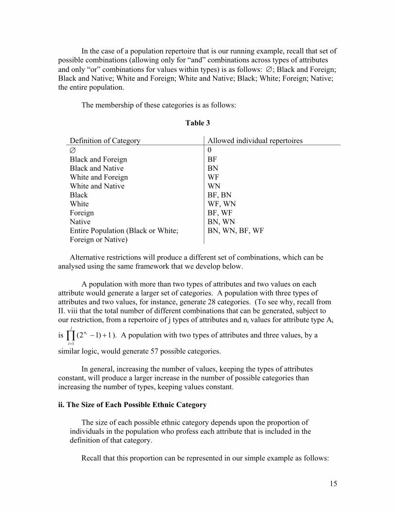
In the case of a population repertoire that is our running example, recall that set of possible combinations (allowing only for “and” combinations across types of attributes and only “or” combinations for values within types) is as follows: ∅; Black and Foreign; Black and Native; White and Foreign; White and Native; Black; White; Foreign; Native; the entire population.

The membership of these categories is as follows:

Table 3

Definition of Category Allowed individual repertoires ∅ 0 Black and Foreign BF Black and Native BN White and Foreign WF White and Native WN Black BF, BN White WF, WN Foreign BF, WF Native BN, WN Entire Population (Black or White; Foreign or Native)

BN, WN, BF, WF

Alternative restrictions will produce a different set of combinations, which can be

analysed using the same framework that we develop below. A population with more than two types of attributes and two values on each

attribute would generate a larger set of categories. A population with three types of attributes and two values, for instance, generate 28 categories. (To see why, recall from II. viii that the total number of different combinations that can be generated, subject to our restriction, from a repertoire of j types of attributes and ni values for attribute type Ai

is ∏ ). A population with two types of attributes and three values, by a

similar logic, would generate 57 possible categories.

1)12(1

+−=

j

i

ni

In general, increasing the number of values, keeping the types of attributes

constant, will produce a larger increase in the number of possible categories than increasing the number of types, keeping values constant.

ii. The Size of Each Possible Ethnic Category

The size of each possible ethnic category depends upon the proportion of

individuals in the population who profess each attribute that is included in the definition of that category.

Recall that this proportion can be represented in our simple example as follows:

15

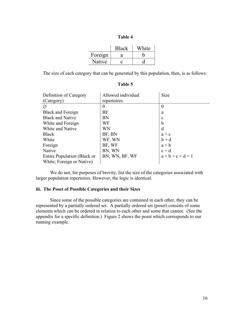
Table 4

Black White

Foreign a b Native c d

The size of each category that can be generated by this population, then, is as follows: Table 5

Definition of Category (Category)

Allowed individual repertoires

Size

∅ 0 0 Black and Foreign BF a Black and Native BN c White and Foreign WF b White and Native WN d Black BF, BN a + c White WF, WN b + d Foreign BF, WF a + b Native BN, WN c + d Entire Population (Black or White; Foreign or Native)

BN, WN, BF, WF a + b + c + d = 1

We do not, for purposes of brevity, list the size of the categories associated with

larger population repertoires. However, the logic is identical. iii. The Poset of Possible Categories and their Sizes

Since some of the possible categories are contained in each other, they can be represented by a partially ordered set. A partially ordered set (poset) consists of some elements which can be ordered in relation to each other and some that cannot. (See the appendix for a specific definition.) Figure 2 shows the poset which corresponds to our running example.

16

Figure 2

BN, WN, BF, WF

BF WN

Ø

WF BN

BF, WF BN, BF WN, WF BN, WN

Each point in the diagram represents a category, described by the individual repertoires that are eligible for membership. In our example, the 10 points represent the membership of the 10 possible categories. At the lowest level we have ∅ and at the highest level we have the entire population.

Categories arrayed at a higher level in the diagram contain some of the categories at a lower level. Each line connecting two points represents containment: when a line connects a lower point to a higher point, the lower category is contained in the higher category. This is illustrated by the thick line in the diagram, which shows that the category White and Foreign, corresponding to the individual repertoire WF, is contained in the category White, which corresponds to the individual repertoires WF and WN. When two categories are not linked by a line, the lower category is not contained by the higher category.

In general, any set of possible categories generated from a repertoire of attributes for

a population can be represented as a poset. The structure of the poset depends upon the number of categories, which is itself derived from the number of types of attributes in the population repertoire and number of values. It will have as many nodes as there are categories. The larger the number of categories, then, the larger and more complicated the poset will be.

For instance, the poset corresponding to a repertoire of attributes for a population that

has three types of attributes and two values on each, for instance, will have 28 nodes. The poset corresponding to a repertoire of attributes for a population that has two types of attributes and three values on each will have 57 nodes. We do not draw out posets corresponding to these larger and more complex population repertoires. But the key point to note here is that we can reduce any number of types of attributes to a two dimensional diagram.

The appendix describes this poset further. For example, we show it is a lattice. We

also determine its structure for any number of types of attributes in the population repertoire and any number of values.

17

iv. The Set Of Minimum Winning Categories The set of minimum winning categories for any population varies with the context.

We can now formally define a context, to mean all of the following information: • the repertoire of salient attributes for the population, • the distribution of the individual repertoires over the population, and • some value k, .5 < k <1, defined as the minimum winning threshold. We take the

value of k to be exogenously determined in the short term.

A category is minimum winning in a context if it fulfils two conditions:

• its size is ≥ k, and • it does not contain any other possible category whose size is also ≥ k. The first condition gives us all categories that are larger than the minimum-winning

threshold. We call this the set of all winning categories. However, as noted above, some possible categories may be contained by others. Individual eligible for membership in two winning categories, one of which is contained by the other, should prefer the smaller one. The second condition captures this logic by including within our set of minimum winning categories only those categories which are “minimal by containment.”

v. Identifying The Set of Minimum Winning Categories in a Poset

The representation of all possible categories using a diagram allows us to identify easily whether a possible category both exceeds the minimum winning threshold k and is minimal by containment.

As an example, suppose k = .6 and suppose that the values of a, b, c and d in our running example are as follows:

Table 6 Black White

Foreign a(.4) b(.4) Native c(.1) d(.1)

Representing this population in Figure 5 shows us immediately that this population

produces only one possible minimum winning category, defined as the category “Foreign”, with membership BF, WF.

18

Figure 5

a+b = .8

a = .4 b = .4 c = .1 d = .1

c+d = .2b+d = .5a+c = .1

0

a+b+c+d = 1

With the same k, consider now the following set of values of a, b, c, and d.

Table 7

Black White

Foreign a(.4) b(.25) Native c(.3) d(.05)

Representing this population in Figure 6 shows us immediately that this population

produces two possible minimum winning categories: one defined “Foreign”, has the membership BF, WF and is of size .7; the other, defined as “Black” has the membership BF and BN and is of size .65. Figure 6 1

.65

.7

.30 .35

.4

.25

.3 .05

0

19

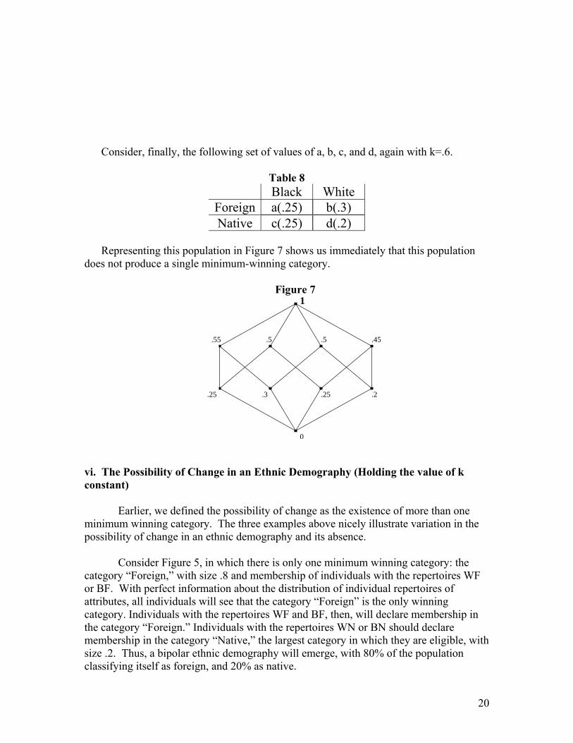
Consider, finally, the following set of values of a, b, c, and d, again with k=.6.

Table 8 Black White

Foreign a(.25) b(.3) Native c(.25) d(.2)

Representing this population in Figure 7 shows us immediately that this population

does not produce a single minimum-winning category.

Figure 7

0

.25

1

.25 .3 .2

.55 .5 .5 .45

vi. The Possibility of Change in an Ethnic Demography (Holding the value of k constant)

Earlier, we defined the possibility of change as the existence of more than one minimum winning category. The three examples above nicely illustrate variation in the possibility of change in an ethnic demography and its absence.

Consider Figure 5, in which there is only one minimum winning category: the category “Foreign,” with size .8 and membership of individuals with the repertoires WF or BF. With perfect information about the distribution of individual repertoires of attributes, all individuals will see that the category “Foreign” is the only winning category. Individuals with the repertoires WF and BF, then, will declare membership in the category “Foreign.” Individuals with the repertoires WN or BN should declare membership in the category “Native,” the largest category in which they are eligible, with size .2. Thus, a bipolar ethnic demography will emerge, with 80% of the population classifying itself as foreign, and 20% as native.

20

Given the winner take all assumption, the payoff for the members of the majority

category will be 100/80=5/4 The payoff for members of the minority category will be 0. Even under such oppressive circumstances, however, individuals with the repertoires WN or BN will not reclassify themselves, since simply do not have any ethnic identity category in their repertoire that will improve their lot. And individuals with the repertoires WF or BF will not reclassify themselves since they cannot do better under a different system of classification. As a result, there is no possibility for change in this ethnic demography as long as the minimum winning threshold remains constant.

Consider now Figure 6, which generates two minimum winning categories: “Foreign”, with size .65 and membership of individuals with repertoires BF or WF; and “Black”, with size .7 and membership of individuals with repertoires BF or BN. In this case, we should expect the initial outcome to be an ethnic demography based on the smaller of these minimum winning categories (Posner 2003). Individuals with the repertoire BF or WF should initially declare membership in the category “Foreign.” This leaves individuals with the repertoire BN or WN no option but to choose the category “Native,” with size .35. A bipolar ethnic demography will emerge, with 65% of the population classifying itself as Foreign, and 35% as Native. The payoff for members of the majority category will be 100/65, while the payoff for members of the minority category will be 0.

In this scenario, the possibility for change in an ethnic demography does exist,

driven by those who stand to lose under one scheme of categorization but can gain in another. In this scenario, individuals with the repertoire BN can induce a change to a new ethnic demography by giving those with the repertoire BF an incentive to reclassify themselves as “Black” rather than “Foreign.” Note that they can only do this if they offer the BFs some portion of their own expected payoff as a side-payment, and so increase the individual payoff for a BF beyond 100/65. We should expect those with the repertoire WF also to make a counter-offer, surrendering a portion of their payoffs to keep the BF in the category “Foreign” and preserve the status quo. The outcome depends on which of these two sections of the population make a more attractive offer.

We do not develop here a theory of individual entrepreneurship which would allow us to predict whether the possibility of change in this scenario is actually realized. The maximum side payment that individuals who share the same repertoire are able to offer is bounded by their total share of the payoff. In the example above, for instance, the maximum side-payment that the BNs or WFs can offer is their total share of the payoff: (100*30/70) in the case of the BNs, and (100*25/65) in the case of the WFs.9 But their ability to offer sidepayments at all, and if so, the difference between their offers depends upon variables that we do not theorize about here.

9 There may be conditions in which, even when more than one minimum winning category exists, the difference in sizes is such that even the maximum possible side-payment does not exceed the minimum that would be necessary to induce a switch. We have not identified these conditions.

21

These variables include, among others, ability to coordinate (if they are not able to coordinate, they will not be able to make an offer); differences in the way that they organize themselves (a centralized decision-making structure may be able extract more resources from its members and so offer a greater side payment than a competitive one); the degree of internal competition among those who share the same repertoire (more competition may reduce the amount of side-payment as rivals “bid up” the payoff that they promise to retain); in institutional strength (strong institutions may induce individuals to have longer time horizons and so offer greater side payments in the present than weak institutions) etc.

Indeed, we do not think it is advisable to propose such a theory at the level of

generality that we aim for here. The extent to which individuals are able to coordinate, and the particular forms that such coordination take, may vary with the particular context in which the game is played. We aim here simply to show, using minimal assumptions, that the possibility of change exists. Whether or not this possibility is realized will depend upon additional assumptions and restrictions imposed on a context-by-context basis. Finally, consider the example in which the distribution of individual repertoires fails to generate any minimum winning category, as in the case of Figure 7. In this scenario, we should expect individuals to include salient non-ethnic attributes in their quest for a minimum winning category. The result will be the emergence of a demography composed of categories that are either defined entirely by non-ethnic attributes or in which non-ethnic attributes are combined with ethnic attributes. We term this a non-ethnic demography.10 vii. Predicting the Possibility of Change in an Ethnic Demography (Allowing the Value of k to Vary)

Above, we predicted the possibility of change in an ethnic demography holding the value of k constant. But another way to think about the possibility of change in an ethnic demography is to explore the extent to which an ethnic demography is robust to changes in the value of k.

For example, consider the population described in Figure 5. For this distribution of

attributes, we see from Figure 5 that the ethnic demography will remain unchanged for a large range of values of k (.5 < k ≤ .8). For any k value in this range, the ethnic demography will be composed of a “Foreign” majority of 80% and a “Native” minority of 20%. Once the value of k exceeds .8, this population will not generate any minimum winning ethnic category.

The ethnic demography in Figure 5 is more stable across contexts than the ethnic

demography in Figure 8 below.

10 Strictly speaking, this is a residual category that includes all those categories not purely defined by ethnicity (e.g. white and poor). A term other than non-ethnic demography might be preferable here.

22

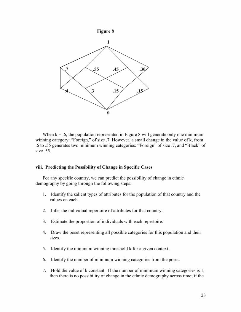
Figure 8

1

.7

.55

.45 .30

.4

.3

.15 .15

0

When k = .6, the population represented in Figure 8 will generate only one minimum

winning category: “Foreign,” of size .7. However, a small change in the value of k, from .6 to .55 generates two minimum winning categories: “Foreign” of size .7, and “Black” of size .55. viii. Predicting the Possibility of Change in Specific Cases

For any specific country, we can predict the possibility of change in ethnic demography by going through the following steps:

1. Identify the salient types of attributes for the population of that country and the values on each.

2. Infer the individual repertoire of attributes for that country.

3. Estimate the proportion of individuals with each repertoire.

4. Draw the poset representing all possible categories for this population and their

sizes.

5. Identify the minimum winning threshold k for a given context.

6. Identify the number of minimum winning categories from the poset.

7. Hold the value of k constant. If the number of minimum winning categories is 1, then there is no possibility of change in the ethnic demography across time; if the

23

number of winning coalitions is greater than one, then there is a possibility of change; and if the number of minimum winning categories is 0, we should expect a salient non-ethnic demography.

8. Now vary the value of k. The greater the range of values of k for which the

number of minimum winning categories is 1, the more robust this ethnic demography is to change across context.

ix. Predicting the Possibility of Change in General

Can we say anything about the possibility of change associated with population repertoires of different sizes and composition? Are large population repertoires more likely to be associated with distributions of individual repertoires that produce the possibility of change than small ones? Are population repertoires with a small number of types but a large range of values over these types more likely to produce the possibility of change than population repertoires with a large number of types but a small range of values over these types? Let us first discuss the possibility of change associated with the population repertoire in our running example, with 2 types of attributes and two values on each type. Four distinct individual repertoires can be generated from this population repertoire, and these four repertoires can be distributed in varying proportions across a population. Chart 7 summarizes the proportion of these distributions that produce, for different (discrete) values of k, a stable ethnic demography, defined here as producing exactly one minimum winning category (Line 1); the possibility of change in an ethnic demography, defined here as producing more than one minimum winning category (Line 2); and a non-ethnic demography, defined here as producing no minimum winning category (Line 3).

24

Chart 7Population Repertoire: 2 Types, 2 Values on Each

No. of Individual Repertoires: 4

0

0.1

0.2

0.3

0.4

0.5

0.6

0.7

0.8

0.9

1

0.5 0.55 0.6 0.65 0.7 0.75 0.8 0.85 0.9 0.95 1

K (Minimum Winning Threshold)

Prop

ortio

n of

Dis

trib

utio

ns o

f In

divi

dual

Rep

erto

ires

1 Stable Ethnic Demography(Exactly One MWC)

2 Possibility of Change inEthnic Demography (Morethan One MWC)

3 Non-Ethnic Demography (NoMWC)

1

2

3

For low to moderate values of k (.5 < k ≤ 73), this population repertoire is more likely to produce a stable ethnic demography than any other outcome. However, for high values of k, ( .73 < k <1), a non-ethnic demography becomes the more likely outcome. The proportion of distributions that generates the possibility of change in an ethnic demography also decreases with increasing values of k. However, it is always less likely than one of the other two outcomes.

Another way to interpret this chart is as follows: As the value of k increases,

distributions of individual repertoires that generate any minimum winning category become increasingly rare. But when a distribution of individual repertoires does generate a minimum winning category, the probability that this will be a unique one is high.

What does this mean about the possibility of change in the ethnic demographies in particular countries with a population repertoire of 2 types of attributes and 2 values on each type? In order to extrapolate from this graph to countries that have such a population repertoire, we need to know how different distributions of individual repertoires are distributed across these countries. In the absence of further information, we make the assumption that these distributions are randomly countries are randomly distributed across countries. Given this assumption, we can infer that the probability that these countries will generate the possibility of change in their ethnic demographies is generally low for all values of k. For these countries, we should be most likely to see stable ethnic demographies for low to moderate values of k (.5 < k ≤.73), and non-ethnic demographies for high values of k (.73 < k <1). (Note, however, that this inference

25

would not hold if the distribution of individual repertoire of attributes across countries were skewed.)

Consider now what happens when we hold constant the number of types of attributes in a population repertoire but increase the number of values on each type from 2 to 3. This population repertoire generates a total of 9 distinct individual repertoires that can be distributed in different proportions across a population. Chart 8 summarizes the proportion of these distributions that produce, for different values of k, a stable ethnic demography; the possibility of change in an ethnic demography; and a non-ethnic demography.

Chart 8Population Repertoire: 2 Types, 3 Values on Each

No. of Individual Repertoires: 9

0

0.1

0.2

0.3

0.4

0.5

0.6

0.7

0.8

0.9

1

0.5 0.55 0.6 0.65 0.7 0.75 0.8 0.85 0.9 0.95 1

K (Minimum Winning Threshold)

Prop

ortio

n of

Dis

trib

utio

ns o

f Ind

ivid

ual

Rep

erto

ires

1 Stable Ethnic Demography(Exactly One MWC)

2 Possibility of Change in EthnicDemography (More than OneMWC)

3 Non-Ethnic Demography (NoMWC)

1

2

3

The first thing to note about this population repertoire is that it generates a much higher likelihood of the possibility of change in an ethnic demography than the previous one. For low to moderate values of k (.5 < k ≤ .77), the possibility of change is more likely than any other outcome. For a small interval ( .78 < k ≤ .83, the proportion of distributions that generate stability is more likely than any other outcome. And for high values of k (.83 < k < 1), a non-ethnic demography becomes the more probable outcome.

Making as above the assumption that these distributions are randomly distributed across countries, we can infer that for low to moderate values of k, countries with this type of population repertoire should be more likely to have the possibility of change in their ethnic demographies than any other outcome. At high k values, we should find non-

26

ethnic bases for coalition building. Stable ethnic demographies in such countries are unlikely except for a brief window when k is moderately high.

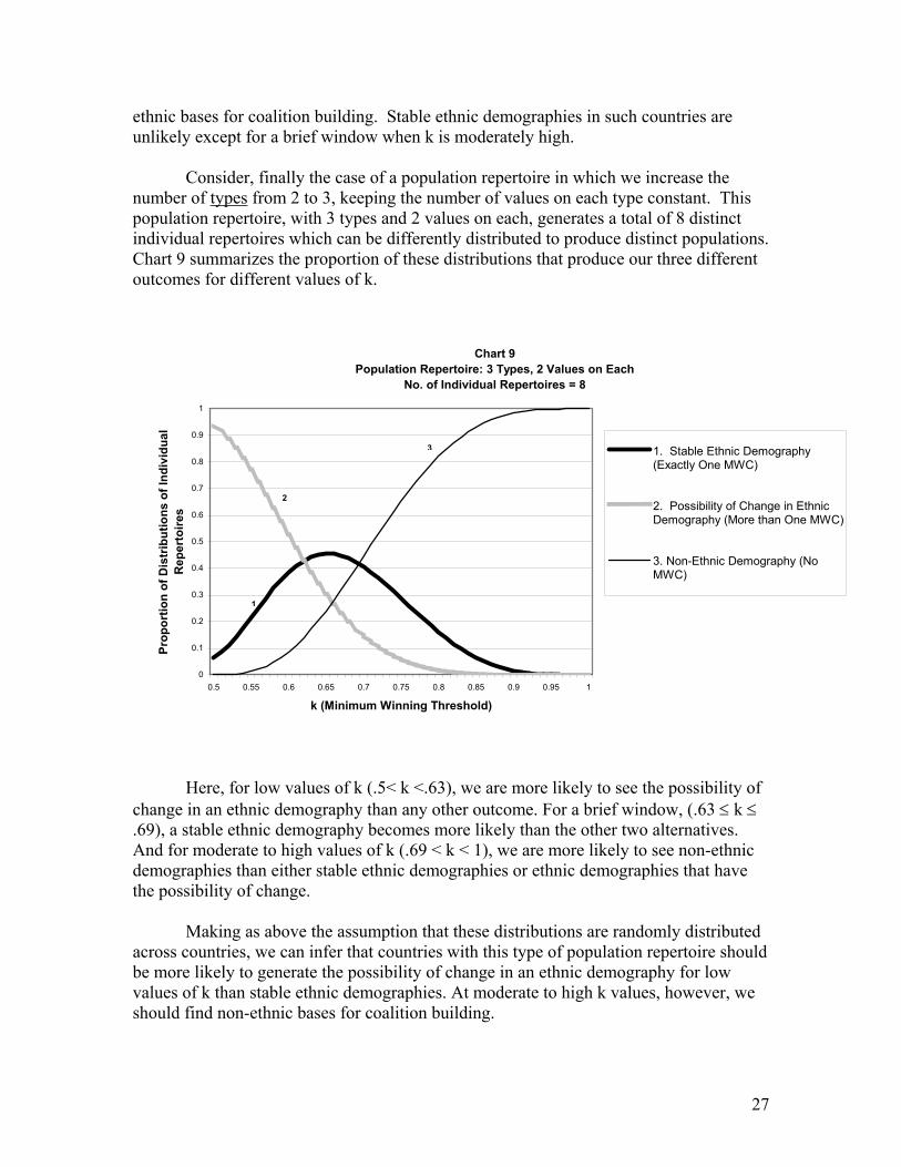
Consider, finally the case of a population repertoire in which we increase the

number of types from 2 to 3, keeping the number of values on each type constant. This population repertoire, with 3 types and 2 values on each, generates a total of 8 distinct individual repertoires which can be differently distributed to produce distinct populations. Chart 9 summarizes the proportion of these distributions that produce our three different outcomes for different values of k.

Chart 9Population Repertoire: 3 Types, 2 Values on Each

No. of Individual Repertoires = 8

0

0.1

0.2

0.3

0.4

0.5

0.6

0.7

0.8

0.9

1

0.5 0.55 0.6 0.65 0.7 0.75 0.8 0.85 0.9 0.95 1

k (Minimum Winning Threshold)

Prop

ortio

n of

Dis

trib

utio

ns o

f Ind

ivid

ual

Rep

erto

ires

1. Stable Ethnic Demography(Exactly One MWC)

2. Possibility of Change in EthnicDemography (More than One MWC)

3. Non-Ethnic Demography (NoMWC)

1

2

3

Here, for low values of k (.5< k <.63), we are more likely to see the possibility of change in an ethnic demography than any other outcome. For a brief window, (.63 ≤ k ≤ .69), a stable ethnic demography becomes more likely than the other two alternatives. And for moderate to high values of k (.69 < k < 1), we are more likely to see non-ethnic demographies than either stable ethnic demographies or ethnic demographies that have the possibility of change.

Making as above the assumption that these distributions are randomly distributed across countries, we can infer that countries with this type of population repertoire should be more likely to generate the possibility of change in an ethnic demography for low values of k than stable ethnic demographies. At moderate to high k values, however, we should find non-ethnic bases for coalition building.

27

We have not experimented with larger increases either in the number of values on each type, keeping the number of types constant, or in the number of types. Our expectation is that increases in either will dramatically lower the probability of stability in an ethnic demography. There may be a cutoff point beyond which no distributions of individual repertoires will produce stability.

However, there should be differences in what we see in place of stable ethnic

demographies. Increasing the range of values on each type, keeping the number of types constant, should, we expect, produce a greater tendency towards the possibility of change in an ethnic demography than towards the emergence of a non-ethnic demography, even at high values of k. But increasing the number of types of attributes, keeping values constant, should produce a greater tendency towards non-ethnic demographies. III. Limitations and Extensions

We discuss here several limitations in the model in its current form and some extensions. We propose to undertake two of these extensions ourselves, and hope that that contributors to this volume might consider others.

First, this model applies only to winner-take-all situations in which the outcome is determined by majority rule. We do not explore the possibility of change associated either with other decision rules in a winner-take-all system (e.g. plurality rule) or with systems that are not winner-take all (e.g. in which the payoff is distributed proportionally among groups). We expect in a second draft to extend this model to include these other decision rules.

Second, it applies only to situations in which the payoffs are individually divisible among members of the winning category. This captures an important class of phenomena in which ethnic identities are likely to be relevant (Brass, Posner, Chandra, Laitin, Melson and Wolpe, Kasfir, Fearon, Caselli). But we do not have anything to say about the outcome when the rewards are collectively distributed. Extending the model to cover this class of situations is our next priority in revisions to this model.

Third, without a theory of how the set of salient attributes can be determined, this model is able to explain change in an ethnic demography but not necessarily its origins. If the ethnic attributes that are included in the set of salient attributes are initially “free-floating,” then we can explain the origin of an ethnic demography as the product of the first round of choice outlined above, and change in an ethnic demography as the product of subsequent rounds of choice. But, it may also be the case that ethnic attributes become salient because they are embedded within the categories of an initial ethnic demography for whose origin we do not have an explanation. In this case, even the first round of choice in our model represents change rather than origin. We see this as a necessary limitation. We have to start somewhere, and it may not be possible here to start at the beginning. But, given some arbitrarily determined starting point, we can always predict the possibility of change.

28

Fourth, instead of treating all permissible identity categories as having equal weights, as we have done, extensions of the model might weight them differently in at least two ways:

● Weighting types of attributes differently: By imposing different initial weights on

types of attributes, we can generate identity categories that are of different values. Imposing such weights is one way to capture the lower value of categories defined by stigmatized types of attributes (Petersen 2002); or the higher value of categories defined by types of attributes that are more visible; or more “sticky;” or institutionally privileged etc.

● Weighting combinations of attributes differently: In our description of an identity

repertoire, we eliminate very complex combinations on the grounds that individual cognitive capacities are limited. An extension of this model might weight combinations by their degree of complexity. This may be desirable if we believe that individuals are driven by necessity to become more sophisticated: They may initially favour simple combinations, and progress to more complex ones if these simple combinations do not generate a winning option.

Fifth, extensions to the model might consider modifying our assumption about

information. This version of the model requires individuals to have perfect information about the distribution of individual repertoires and the range of coalitions of different sizes that are derived from this distribution. Less demanding assumptions about information include the following:

• Individuals have information about the range in which individual repertoires of

attributes are distributed rather than exact proportions. • There may be variation in the reliability of information associated with different

types of attributes. We could model this by associating different types of attributes with different degrees of error and allotting weights accordingly.

• Individuals have information about the proportions in which each value on each

type of attribute is distributed in the population but not how these values are combined in individual repertoires (Van Der Veen and Laitin, 2002)

Sixth, while this model assumes an undifferentiated population of individuals,

extensions might differentiate between ordinary individuals and entrepreneurs. One important way in which entrepreneurs can influence identity change is to eliminate possibilities in an identity repertoire. We do not model this process here. However, this model can be used to construct a theory of political entrepreneurship that explains why politicians might use one set of restrictions over another. Such a theory might stand alone or be used to supplement this model to predict the pattern of change in particular contexts.

29

Finally, while we take the distribution of attributes as fixed, extensions might consider how the introduction of new attributes, other things equal, affects the possibility of change. IV Implications for Theories Using Ethnic Demography As an Independent Variable

The first implication, not only of this model but of the broader constructivist

literature on which it is based, is that ethnic demography cannot be treated as an acontextual variable. Instead of asking what the impact of ethnic demography is on dependent variable X, these theories must ask: What is the impact of the ethnic demography in some particular context on dependent variable X? (Laitin and Posner 2001).

For example, research on the relationship between ethnic demography and economic growth must explain whether it is interested in the effect of the ethnic demography that is salient in the context of the national (or subnational) census; or the ethnic demography that is salient in the context of national (or subnational) political party competition; or the ethnic demography as salient in the arena of national (or subnational) economic policy making etc.

It may well be that for some countries, there is little change in the ethnic

demography across these contexts. This would correspond in our model either to a situation in which the minimum winning threshold k is invariant across contexts, or a situation in which the number of minimum winning categories is invariant across changing values of k. For these countries, identifying the context within which the ethnic demography is contained would not make a difference to the empirical results. However, it is important for the purpose of constructing a clear theoretical argument.

The remainder of this section discusses how, given some context, we can use this

model to determine whether and to what extent fluidity or endogeneity poses a problem for the outcome under consideration. Finally, it identifies some of the new questions that this model allows us to ask and answer. i. Fluidity

Research on ethnic demography as an independent variable uses three different summary measures to describe an ethnic demography: the ELF index; the size of the largest group; and the difference between the two largest groups. The ELF index measures the degree of ethnic “diversity” or “heterogeneity.” The latter two measures measure the extent to which a system is majority dominated (Bates, Fearon).

The model here allows us to estimate the maximum change in these measures (and

others) for particular populations. Once we know the maximum change in any of these measures for all countries in a dataset, we can determine the magnitude and direction of bias in an econometric analysis that does not take fluidity into account.

30

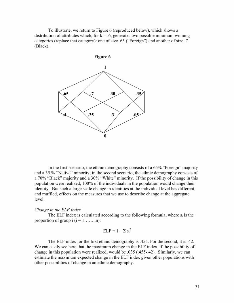
To illustrate, we return to Figure 6 (reproduced below), which shows a distribution of attributes which, for k = .6, generates two possible minimum winning categories (replace that category): one of size .65 (“Foreign”) and another of size .7 (Black). Figure 6

1

.65

.7

.30 .35

.4

.25

.3 .05

0

In the first scenario, the ethnic demography consists of a 65% “Foreign” majority

and a 35 % “Native” minority; in the second scenario, the ethnic demography consists of a 70% “Black” majority and a 30% “White” minority. If the possibility of change in this population were realized, 100% of the individuals in the population would change their identity. But such a large scale change in identities at the individual level has different, and muffled, effects on the measures that we use to describe change at the aggregate level. Change in the ELF Index

The ELF index is calculated according to the following formula, where si is the proportion of group i (i = 1……..n):

ELF = 1 – Σ si2

The ELF index for the first ethnic demography is .455. For the second, it is .42.

We can easily see here that the maximum change in the ELF index, if the possibility of change in this population were realized, would be .035 (.455-.42). Similarly, we can estimate the maximum expected change in the ELF index given other populations with other possibilities of change in an ethnic demography.

31

Change in the Size of the Largest Group In this example, the maximum change in the size of the largest group for this

population, taking the absolute value of the difference between the first winning category and the second, is .05. By the same logic, we can calculate the maximum change in this measure for a population with any number of minimum winning categories by subtracting the smallest of these categories from the largest. Difference in the Size of the Two Largest Groups.

For this example, the difference between the two largest categories in the first ethnic demography is .3 (.65-.35), and in the second ethnic demography, it is .4 (.7-.3). The maximum change possible in this measure, taking the absolute value of the difference of the two values, is .10.

In general, we expect that the maximum expected change in any of these

measures will be small when the minimum winning threshold is constant. This is because the size of the largest category, and therefore the size of the residual categories, is likely to fluctuate within only a limited range. Changes in the size of the minimum winning threshold may produce greater changes in each of these measures. Difference in the Type of Attributes Activated

Finally, we can use the model to estimate the maximum degree of fluidity in the type of attributes activated, even when the size of the activated categories does not change.

This type of fluidity is important because of a recently developing line of questioning within the literature on ethnic politics that asks whether some types of attributes (e.g. religion) are associated with different political consequences than others (e.g., language) (Wilkinson 2002; Laitin, 1999).

Note that we say “types of attributes” here rather than dimensions, as is common

in the literature. This is because the term “dimension,” defined as a “family” of categories, becomes meaningless when we are confronted with categories that are combinations of multiple types of attributes.

Take for instance a category that combines values on two types of attributes:

“Black and Native.” Or three: “Black and Native and Tall.” There is no meaningful “family” on which we can arrange such categories, although we might make one up.

By using the term “type of attribute,” we compare fluidity in the inputs used in the

construction of categories without making any assumption that the outputs, i.e. the categories themselves are arranged in some meaningful family.

32

ii. Endogeneity The two principal determinants of an ethnic demography in our model are the minimum winning threshold k and the underlying distribution of individual repertoires of attributes. We can say, therefore that theories investigating the impact of ethnic demography on some outcome X faces an endogeneity problem to the extent that this outcome affects either the value of k or the distribution of the individual repertoires of attributes.

For example, suppose we are interested, following Ordeshook and Shvetsova, in

studying the impact of ethnic demography on the number of parties. Suppose, following our injunction to identify the context within which our ethnic demography of interest is contained, we stipulate that we are interested in exploring the effect of ethnic demography as described in the national level census of each country.

The next step is to ask whether the size threshold k that individuals consider when

classifying themselves in census forms is likely to be affected by the number of parties. Our intuition is that there may be a relationship between the two. In two-party systems, ethnic groups need to be larger in order to be influential than in multi-party systems. The census is the principal means by which individuals can convey information about their own group size, and obtain information about the relative sizes of other groups. Consequently, we should expect individuals in two party systems to classify themselves in larger categories in the national level census than individuals in multi-party systems.

We do not expect there to be a significant relationship between the number of parties

and the distribution of individual repertoire of attributes in the population. But entrepreneurs in two party systems may restrict the choice set of categories in the census to induce individuals to identify in larger rather than smaller categories.

Here, our model allows us to determine how much difference this possible reverse

causal link might make. If the underlying distribution of individual repertoires of attributes does not permit individuals in our country of interest much room for reclassification, then even though the possibility of endogeneity exists, it is not likely to make much difference to our model. However, if the underlying distribution of individual repertoires of attributes does permit individuals substantial room for reclassification, then endogeneity poses a more serious challenge to the analysis. iii. Generating New Questions So far, our focus has been on showing how the model might be used to identify whether fluidity and endogeneity pose a problem for old theories relating ethnic demography (given some context) to some dependent variable X. But constructivist approaches also generate new questions that could not have been asked before (Lustick 2001). This section speculates about some of the new questions that this model allows us to ask and answer.

33

Electoral Systems One way to define electoral systems is to think of them as devices that set a

minimum winning threshold in a given context. Holding the distribution of individual repertoires of attributes constant, this model allows us to ask: What electoral system will be optimal given the distribution of identity repertoires in a population?

Individuals with the power to determine the choice of electoral system should,

other things equal, choose that value of k that maximizes the probability of producing a unique minimum winning category in which they are eligible for membership. By comparing the different outcomes that individuals with some given repertoire of attributes might obtain under different values of k, we can predict that value of k that they should find optimal.

Note that the insight that individuals will choose an electoral system that is optimal for them is itself unremarkable. We know for instance that ethnic minority groups are likely to prefer proportional electoral systems, while ethnic majority groups are likely to prefer first past the post electoral systems. The contribution of this model is making it possible to ask and answer the question of what institutional arrangement is optimal for some set of individuals, given not only their currently activated identities, but also their large repertoire of potential identities. Boundaries of the Political Arena

Changes in the boundaries of the political arena can allow disadvantaged individuals to reverse their situation (Posner 2003). Such changes include federalism, the delimitation of electoral constituencies, and the rules for the composition of executives and legislatures.

Any of these institutional changes can alter some individuals’ prospects of

winning by effectively redistributing individual repertoires of attributes in new compartments or partitions. The model allows us to determine which partitions of the population will produce a unique minimum-winning category for some set of individuals. As such, it should allow us to predict their preferences over different boundary arrangements and identify the most likely outcome. Compliance and Violence We know that compliance should be most likely under those institutional arrangements in which all individuals have some expectation of being in a winning position. Conversely, violence is most likely when some individuals are likely to be consistent losers.

The model allows us to determine the space within which compliance can be induced, holding the distribution of attributes constant, by determining the range of minimum winning thresholds that will produce permanent losers. Alternatively, it can also be used to explore the ways in which the population can be partitioned to change previous losers into winners.

34

Violence, then, should be most likely for that limited set of cases in which the repertoires of attributes for some set of individuals is such that they are likely to be losers given not only currently activated identities and current institutions, but also under all other imaginable identities and institutional arrangements. V. Suggestions for Contributors to the Volume We think of this chapter as the prelude to the heart of the volume: the chapters that incorporate constructivism into dependent variable X. Contributors to these chapters might proceed in one of three ways: First, you may find that this model captures enough of the essential features of the context that you are analyzing that you use it to develop a constructivist theory for your dependent variable X without modification. Even so, however, you will need to supplement the model with additional assumptions about individual behaviour that will let you determine when and why the possibilities of change are realized.

Second, you may find that that this model requires modification before it can be used to develop a constructivist theory for your dependent variable. In this case, we encourage you to modify the model as necessary, identifying and justifying the modifications along the way.

Third, you may find that this model is not applicable for your particular problem.

There are several areas where this might be the case. One, as we noted in Section III, consists of those situations in which individuals are concerned with collective rather than individual benefits. Another consists of those situations in which individual ethnic identifications are a matter of imposition rather than choice. In such cases, we encourage you to develop an alternative model, making explicit your points of departure and your basis for doing so.

The goal is to produce a theoretically integrated volume that proposes

constructivist theories of politics. But this theoretical integration can come about either through agreement or through explicit and cumulative disagreement.

35

Chart 1Rwanda's Ethnic Demography

(1978 Census)

Hutu91.5%

Tutsi7.9%

Twa0.4%

Other0.2%

Chart 2Rwanda's Ethnic Demography

(1991 Census)

Hutu91.5%

Twa0.4%

Other0.2%Tutsi

7.9%

36

Chart 3Brazil's Ethnic Demography

(1940 Census)

Branco (White)63%

Preto (Black)15%

Pardo (Mixed or Brown)21%

Amerelo (Yellow)1% Missing

0%

Chart 4Brazil's Ethnic Demography

(1991 Census)

Branco (White)53%

Preto (Black)5%

Pardo (Mixed or Brown)42%

Amerelo (Yellow)0%

Indigena (Indigenous)0%

Missing0%

37

Chart 5Sri Lanka's Ethnic Demography

(1953 Census)

Low Country Sinhalese42%

Kandyan Sinhalese27%

Ceylon Tamils11%

Indian Tamils12%

Ceylon Moors6%

Other2%

Chart 6Sri Lanka's Ethnic Demography

(1981 Census)

Sinhalese73%

Sri Lanka Tamil13%

Indian Tamil6%

Sri Lanka Moor7%

Other1%

38