Computers and Structures 117 (2013) 95–104

Contents lists available at SciVerse ScienceDirect

Computers and Structures

journal homepage: www.elsevier .com/locate /compstruc

A method for enhancing computational efficiency in Monte Carlocalculation of failure probabilities by exploiting FORM results

0045-7949/$ - see front matter � 2012 Elsevier Ltd. All rights reserved.http://dx.doi.org/10.1016/j.compstruc.2012.11.022

⇑ Corresponding author.E-mail addresses: jehurtadog@unal.edu.co (J.E. Hurtado), daalvarez@unal.edu.co

(D.A. Alvarez).

Jorge E. Hurtado ⇑, Diego A. AlvarezUniversidad Nacional de Colombia, Sede Manizales. Apartado 127, Manizales, Colombia

a r t i c l e i n f o

Article history:Received 8 October 2011Accepted 20 November 2012Available online 29 December 2012

Keywords:Structural reliabilityFORMReliability plotMonte Carlo simulation

a b s t r a c t

The First-Order Reliability Method (FORM) is by far the most widely employed method for structural reli-ability computation. Its accuracy, however, is fair only when the curvature of the limit state function isvery mild. In this paper, a reliability method built on the design point vector given by FORM is proposed.It is based on the computation of the limit state function of a relatively small selected set of Monte Carlosamples that have the highest similarity to the design point in a statistical sense. The similarity is mea-sured by two nonlinear features extracted from the mass of input variable realizations. The bi-dimension-ality of the mapping allows a simple visual selection of the highly relevant samples and the relevantsample selection is facilitated by the fact that the failure domain possesses a standard shape in the spacespanned by those nonlinear features and also by the feasibility of mapping several possibilities of a sec-ond-order approximation of the limit state function onto the plot, which embrace the most relevant sam-ples. The method yields the same estimate of the failure probability as the simple Monte Carlo, with acomputational cost limited to the evaluation of a subset of the selected samples. Besides, the reductionof the variability of the probability estimates is easily accomplished. Its application is illustrated withsome numerical examples derived from actual structural engineering practice. They show that themethod is simple, efficient and elegant, as it allows visualizing the reliability problem in the plot consti-tuted by the two nonlinear features.

� 2012 Elsevier Ltd. All rights reserved.

1. Introduction

As is well known, the basic problem of structural reliability canbe defined as the estimation of the probability mass of a failure do-main F defined by a limit state function g(x) of a set of input ran-dom variables X of size d. The complement to the failure domain iscalled the safe domain S. In transforming the variable set x to thestandard Gaussian set u, using techniques such as the Nataf model[1,2], Hermite polynomials [3] or others, the problem reads (seee.g. [4,5])

Pf ¼ZF

pUðuÞdu ð1Þ

where pU(u) is the joint probability density function of the basicvariables in the d-dimensional space u. In performing this transfor-mation the limit state function g(x) is transformed into a functiong(u) � g(T(x)), where T(�) is a probabilistic transformation, and thefailure domain becomes F ¼ fu : gðuÞ 6 0g.

The First-Order Reliability Method (FORM) is by far the mostwidely employed method for structural reliability computation. It

is formulated in the standard Gaussian space u and is based onconcepts reflecting the structural safety problem in a clear manner.In addition, several efficient algorithms have been proposed for itsapplication, some of which have been incorporated in commercialsoftware.

The FORM estimate of the failure probability is

Pf ;FORM ¼ Uð�bÞ ð2Þ

where U(�) is the standard Gaussian distribution and b is the mini-mum distance from the origin to the limit state function g(u). It isfound by solving optimization problem:

uH ¼ arg min kuk subject to gðuÞ ¼ 0: ð3Þ

This implies that b = kuwk and the point uw is referred to as the de-sign point.

In the last decades several algorithms have been proposed forsolving this optimization problem (see [6–8] and [9], which con-tains a recent state-of-art on this subject). The accuracy of theprobability estimate given by Eq. (2) is, however, restricted to limitstate functions whose curvature and hence their departure fromlinearity is very small, as determined quantitatively by [10]. Thelimited accuracy of FORM has also been studied by many otherresearchers (see e.g. [11–17]).

Fig. 1. FORM and the polar features of Gaussian samples.

96 J.E. Hurtado, D.A. Alvarez / Computers and Structures 117 (2013) 95–104

In addition, the FORM index b (also known as the Hasofer–Lindindex) has been criticized for not satisfying the requirements ofglobality and ordering, which are expected from any measure in-tended to serve as a reliability index [11]. Under the former expres-sion it is meant that such an index should ideally be a globalmeasure of the reliability associated to the entire safe domain andnot be tied to a local detail of the limit-state function. The Haso-fer–Lind index fails to satisfy this requirement, as it is tied to a sin-gle point. On the other hand, the ordering is a desirable property ofany reliability index, for one expects that to safe domains forming anested sequence S1 � S2 � S3 � � � � there corresponds a similarnested sequence of indexes b1 < b2 < b3 < � � �. The failure of the Haso-fer–Lind index to meet this requirement is evident in the case ofmutually tangent limit state functions at the common design point,for all of which the index will be the same, in spite of the differencesin failure probability mass. This drawback is due to the fact that theindex is defined as a distance to the limit-state function and thus ithas only a point-wise relationship.

Besides, the expression design point perhaps conveys the mean-ing that it marks the minimum realization u that determines thecrossing from the safety state to the failure one. In other words,it can be interpreted from the structural point of view as the crit-ical realization of the basic variables. However the actual realiza-tions of u that are the closest to the origin of coordinates arelocated at farther distances from uw as the number of dimensionsof the problem d increases [17]. This means that for large d theaforementioned structural interpretation and even its worth havebecome disputable [16–18].

However, in spite of all these shortcomings, this paper demon-strates that the design point vector, being a purely geometrical ele-ment without any intrinsic probabilistic meaning, as theaforementioned derivation shows, is a very powerful device forvisualizing the clustering of Monte Carlo samples in the failure do-main even for high dimensional spaces and solving the reliabilityproblem. Such geometrical meaning is by far more important thanthe usual interpretation as a critical realization, which is valid onlyfor low d, or any other probabilistic interpretation. Therefore, inspite of the limited worth of FORM for reliability estimation[10,11,16,17], the design point it yields is the cornerstone for visu-alizing and hence greatly simplifying the reliability problem andfacilitating its solution.

In this respect, due mention must be given to the fact thatsuch geometrical value of the design point has been recentlyexploited for innovative structural reliability methods [17,19–21]. The geometrical insights shown in present paper are in-tended to be a contribution in this direction. In fact, upon the ba-sis of the clustering properties afforded by the design point it isshown that the selection of the important realizations of the basicvariables u that are worth testing is an easy task. This is due tothe fact that, by characterizing the Gaussian realizations withtwo nonlinear features (namely, their distance to the origin andtheir cosine with respect to the design point vector), the failuresamples most naturally accommodate in a corner of the bi-dimensional plot constituted by these two features. The possibil-ity of having such a standard geometrical form allows the isola-tion of a small set of worth-testing samples from a large massof Monte Carlo candidates by simply drawing on the plot somecurves arising from a standard second-order Taylor approxima-tion of the limit state function. Then, after simply counting thesamples lying above the lines, only a portion of them comprisedbetween two of them is actually computed.

The next section is devoted to a detailed exposition of the pro-posed approach for the selection of samples that are worth of eval-uation. This is followed by a section in which the robustness,accuracy and efficiency of the proposed method is demonstratedwith numerical examples. The paper ends with some conclusions.

2. Clustering for selecting highly relevant samples

Let us assume that the reliability problem has been transformedto the space of independent standard Gaussian variables and thatthe FORM problem has been solved. Such a solution yields threepieces of information: The design point uw, the Hasofer–Lindreliability index b and the estimate of the failure probability Pf ;FORM.

The unit vector of the design point is given by

w ¼ uH

kuHk ð4Þ

Consider Fig. 1 which shows the geometrical elements of FORM to-gether with two samples, uf in the failure domain and us in the safedomain. Any sample u is defined by its Cartesian coordinates (u1-

,u2, . . . ,ud) in the d-dimensional space. We propose to change thisd-dimensional characterization of the samples by a bi-dimensionalrepresentation composed by two nonlinear features: (a) Their dis-tance to the origin and (b) the cosine of the angle they make withthe design point vector w. These new variables are given by

v1 ¼ r ¼

ffiffiffiffiffiffiffiffiffiffiffiffiXd

j¼1

u2j

vuut ð5Þ

v2 ¼ cos w ¼ cos\ðw;uÞ ¼ ðw � uÞkwkkuk ð6Þ

Therefore the new representation of the random variables is givenby the mapping v:¼(v1,v2). Notice that these variables togetheroperate a highly nonlinear map u � Rd # v � R2. This operation,however, does not destroy the clustering structure of the samplesin two classes. In fact, the cosine is a measure of the belonging ofthe sample to one of them, because, the higher the cosine, the high-er the possibility of the presence of the sample in the failure do-main. In fact, consider Fig. 2, which shows two vectors w and u.As the separation between them, given by the norm of w � u,diminishes, the projection given by the dot product (w � u) in-creases. Thus, the cosine measures the proximity of the two vectorsand hence their similarity. In addition, it is a normalized measure,as it varies in the range [�1,+1].

Nevertheless, the cosine is not a sufficient indicator of suchbelonging because the samples in the safe domain that are closeto the interclass boundary are also characterized by high cosine val-ues. The distance from the origin, however, complements the co-sine, as the samples in F are necessarily located far from theorigin. Besides, the two features (v1,v2) = (r, cos w) are independent,because a length increase does not affect the cosine, while this latter

Fig. 2. The cosine as a measure of similarity between vectors.

Fig. 4. The reliability plot for a high number of dimensions. Here, the darkboundary indicates the region which holds the images of the samples when mappedto the space spanned by the variables v1 and v2.

J.E. Hurtado, D.A. Alvarez / Computers and Structures 117 (2013) 95–104 97

remains equal if measured with respect with any other co-linearvector.

For these reasons, it is reasonable to expect that the mappingfrom the standard space (u1,u2, . . . ,ud) to the bi-dimensional space(v1,v2) = (r, cos w) yields a visible discrimination of the safe andfailure classes of samples. This fact will be demonstrated in thesequel.

The general shape of the proposed reliability plot is as shown inFigs. 3 and 4 for low and high values of the dimension d, respec-tively. The shape differences that are evident in comparing thesefigures (from a rectangular shape to a circle) are mainly due tothe Chi density function that governs the distance v2 = r, which is[22]

pðr; dÞ ¼ 1C d

2

� �21�d2rd�1 exp � r2

2

� �ð7Þ

which is biased to the left for low d and gradually assuming a close-

to-Gaussian shape as d increases. For this function, lr !ffiffiffiffiffiffiffiffiffiffiffiffiffiffiffiffid� 0:5p

and r2r ! 0:5 as the dimensionality grows. This means that the sam-

ples tend to migrate to a ring of increasing radiusffiffiffiffiffiffiffiffiffiffiffiffiffiffiffiffid� 0:5p

, constantwidth, and decreasing coefficient of variation rr=lr !ffiffiffiffiffiffiffiffiffiffiffiffiffiffiffiffiffiffiffiffiffiffiffiffiffiffiffiffiffi

0:5=ðd� 0:5Þp

. This is one of the reasons explaining the size reduc-tion of the plot as d grows.

Fig. 3. The reliability plot for a low number of dimensions. Here, the dark linerepresents the region that contains the images of the samples when mapped to thespace spanned by the variables v1 and v2.

The other is that the distribution function of the angle w, whichis [23]

pðw; dÞ ¼ sind�2 wR p0 sind�2 wdw

ð8Þ

becomes peaked at w = p/2 even for moderate d, thus approximat-ing the Dirac delta function. This means that the absolute valuesof the cosine close to one become more rare as d grows, thusexplaining why the region of the space that contains the imagesof the samples for large d (the dark boundary) has been depictedsmaller in Fig. 4 than the contour that holds the images of samplesfor low d in Fig. 3 (again the dark curve). Summarizing, for a lownumber dimensions the plot assumes a wide bullet shape withsmall distances and some cosine values close to the bounds[�1,+1], while it takes a smaller, round shape for moderate andlarge d.

Shape differences aside, the most salient characteristic of thisplot is that, irrespective of the dimensionality, the failure samplescluster in the region corresponding to high values of both v1 andmoderate to high values of v2, due to the reasons stated above.Such domain can be roughly represented by a descending line thatstarts at vw, with a trajectory that is problem dependent, where vw

is the representation of the design point in the (v1,v2) = (r, cos w)plot. Evidently, this representation is vH ¼ vH

1 ; vH

2

� �¼ ðb;1Þ. Notice

that the design point vw remains fixed while the failure samplesmove farther away from it as d increases. This explains why diffi-culties and paradoxes are found when exploring high-dimensionalspaces upon the basis of this vector [17], or vectors parallel to it[16]. In fact, such vectors might point to regions in which failuresamples are simply absent.

In order to demonstrate the discrimination capabilities androbustness of the plot, let us consider the second-order approxima-tion gðuÞ of the limit state function g(u) around the point uw:

gðuÞ ¼ gðuHÞ þ rgðuHÞ � ðu� uHÞ þ 12ðu� uHÞTHðu� uHÞ ð9Þ

hererg(uw) stands forrg(u) evaluated at uw. On the other hand, His the Hessian matrix

7 8 9 10 11 12 13−0.4

−0.3

−0.2

−0.1

0

0.1

0.2

0.3

0.4

v1

v 2

Parabolic limit state − d=100

Safe classFailure class

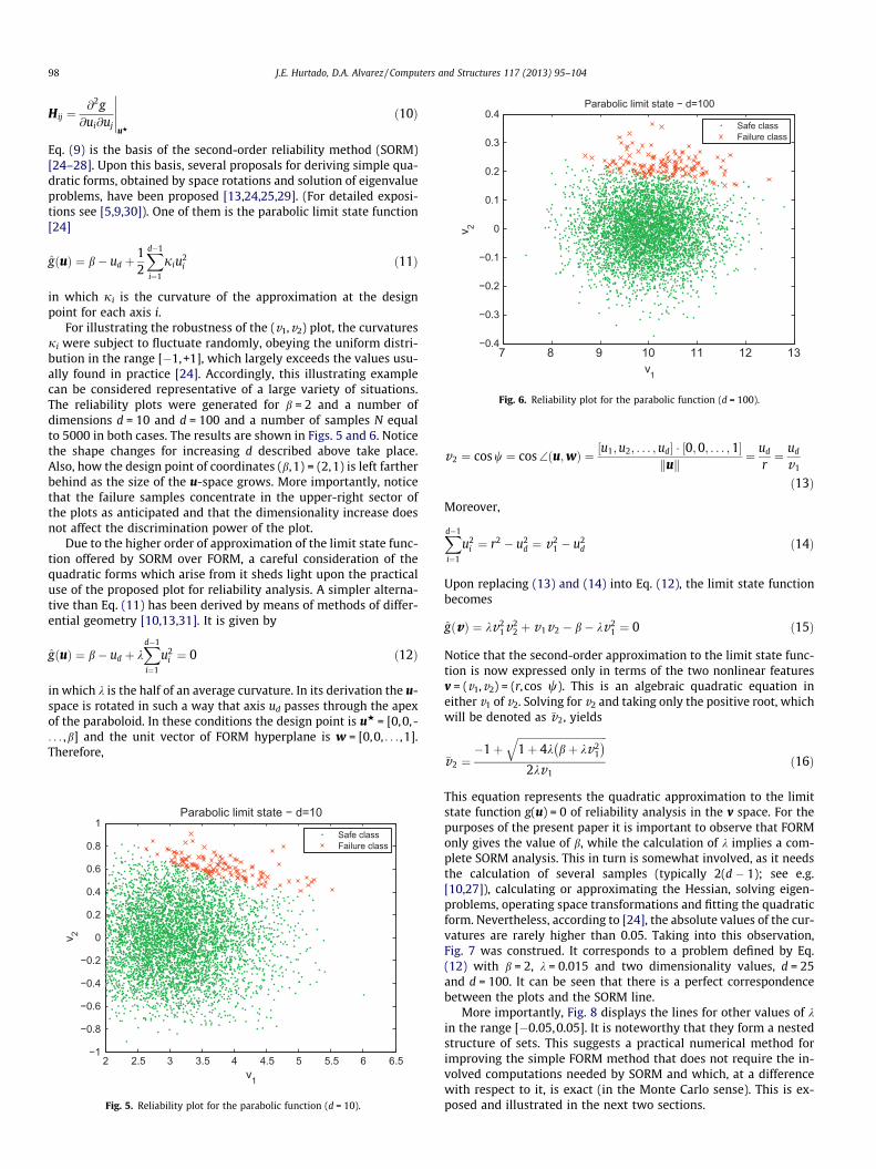
Fig. 6. Reliability plot for the parabolic function (d = 100).

98 J.E. Hurtado, D.A. Alvarez / Computers and Structures 117 (2013) 95–104

Hij ¼@2g@ui@uj

�����uH

ð10Þ

Eq. (9) is the basis of the second-order reliability method (SORM)[24–28]. Upon this basis, several proposals for deriving simple qua-dratic forms, obtained by space rotations and solution of eigenvalueproblems, have been proposed [13,24,25,29]. (For detailed exposi-tions see [5,9,30]). One of them is the parabolic limit state function[24]

gðuÞ ¼ b� ud þ12

Xd�1

i¼1

jiu2i ð11Þ

in which ji is the curvature of the approximation at the designpoint for each axis i.

For illustrating the robustness of the (v1,v2) plot, the curvaturesji were subject to fluctuate randomly, obeying the uniform distri-bution in the range [�1,+1], which largely exceeds the values usu-ally found in practice [24]. Accordingly, this illustrating examplecan be considered representative of a large variety of situations.The reliability plots were generated for b = 2 and a number ofdimensions d = 10 and d = 100 and a number of samples N equalto 5000 in both cases. The results are shown in Figs. 5 and 6. Noticethe shape changes for increasing d described above take place.Also, how the design point of coordinates (b,1) = (2,1) is left fartherbehind as the size of the u-space grows. More importantly, noticethat the failure samples concentrate in the upper-right sector ofthe plots as anticipated and that the dimensionality increase doesnot affect the discrimination power of the plot.

Due to the higher order of approximation of the limit state func-tion offered by SORM over FORM, a careful consideration of thequadratic forms which arise from it sheds light upon the practicaluse of the proposed plot for reliability analysis. A simpler alterna-tive than Eq. (11) has been derived by means of methods of differ-ential geometry [10,13,31]. It is given by

gðuÞ ¼ b� ud þ kXd�1

i¼1

u2i ¼ 0 ð12Þ

in which k is the half of an average curvature. In its derivation the u-space is rotated in such a way that axis ud passes through the apexof the paraboloid. In these conditions the design point is uw = [0,0, -. . . ,b] and the unit vector of FORM hyperplane is w = [0,0, . . . ,1].Therefore,

2 2.5 3 3.5 4 4.5 5 5.5 6 6.5−1

−0.8

−0.6

−0.4

−0.2

0

0.2

0.4

0.6

0.8

1

v1

v 2

Parabolic limit state − d=10

Safe classFailure class

Fig. 5. Reliability plot for the parabolic function (d = 10).

v2 ¼ cos w ¼ cos\ðu;wÞ ¼ ½u1;u2; . . . ;ud� � ½0;0; . . . ;1�kuk ¼ ud

r¼ ud

v1

ð13Þ

Moreover,

Xd�1

i¼1

u2i ¼ r2 � u2

d ¼ v21 � u2

d ð14Þ

Upon replacing (13) and (14) into Eq. (12), the limit state functionbecomes

gðvÞ ¼ kv21v

22 þ v1v2 � b� kv2

1 ¼ 0 ð15Þ

Notice that the second-order approximation to the limit state func-tion is now expressed only in terms of the two nonlinear featuresv = (v1,v2) = (r, cos w). This is an algebraic quadratic equation ineither v1 of v2. Solving for v2 and taking only the positive root, whichwill be denoted as �v2, yields

�v2 ¼�1þ

ffiffiffiffiffiffiffiffiffiffiffiffiffiffiffiffiffiffiffiffiffiffiffiffiffiffiffiffiffiffiffiffiffiffiffi1þ 4k bþ kv2

1

� �q2kv1

ð16Þ

This equation represents the quadratic approximation to the limitstate function g(u) = 0 of reliability analysis in the v space. For thepurposes of the present paper it is important to observe that FORMonly gives the value of b, while the calculation of k implies a com-plete SORM analysis. This in turn is somewhat involved, as it needsthe calculation of several samples (typically 2(d � 1); see e.g.[10,27]), calculating or approximating the Hessian, solving eigen-problems, operating space transformations and fitting the quadraticform. Nevertheless, according to [24], the absolute values of the cur-vatures are rarely higher than 0.05. Taking into this observation,Fig. 7 was construed. It corresponds to a problem defined by Eq.(12) with b = 2, k = 0.015 and two dimensionality values, d = 25and d = 100. It can be seen that there is a perfect correspondencebetween the plots and the SORM line.

More importantly, Fig. 8 displays the lines for other values of kin the range [�0.05,0.05]. It is noteworthy that they form a nestedstructure of sets. This suggests a practical numerical method forimproving the simple FORM method that does not require the in-volved computations needed by SORM and which, at a differencewith respect to it, is exact (in the Monte Carlo sense). This is ex-posed and illustrated in the next two sections.

2 4 6 8 10 12 14−0.8

−0.6

−0.4

−0.2

0

0.2

0.4

0.6

0.8

1

1.2

v1

v 2

Safe classFailure class

d = 25 d = 100

Fig. 7. Reliability plot for the parabolic function for b = 2, k = 0.015 with d = 25 andd = 100, together with the �v2 line.

2 4 6 8 10 12 14−0.8

−0.6

−0.4

−0.2

0

0.2

0.4

0.6

0.8

1

1.2

v1

v 2

d=25d=100λ=−0.02λ=−0.01λ=0.01λ=0.2λ=0.03

Fig. 8. Quadratic form roots for b = 3 and several k, with d = 25 and d = 100.

J.E. Hurtado, D.A. Alvarez / Computers and Structures 117 (2013) 95–104 99

3. The proposed approach

The clustering of the failure samples in a standard zone justdemonstrated allows applying a simple procedure for reliabilitycalculation, consisting in removing the vast majority of Monte Car-lo candidates composing the plot. Initially, a matrix of N standardGaussian random numbers is generated for all input variables. Asis well known, the probability estimates given by the Monte Carlomethod are random variables in themselves, as they are estimatedwith random numbers. The coefficient of variation of the estimatePf of the actual probability Pf is [32]

c:o:v:ðPfÞ ¼

ffiffiffiffiffiffiffiffiffiffiffiffiffi1� Pf

NPf

sð17Þ

An estimate exhibiting a coefficient of variation lower than 0.1 isgenerally accepted as satisfactorily accurate. Since the value of Pf

is normally very small, the numerator of the above expression isclose to one. This means that a large N is needed for reducing theuncertainty on Pf . Therefore, it is proposed to select the number N

such that the coefficient of variation of the failure probability esti-mate, given by Eq. (17), be less than 0.1. This implies that

N > 1001� Pf;FORM

Pf ;FORM

ð18Þ

At this step these random numbers are unlabeled, i.e. it is unknownto which of the safe or failure classes they belong. Since the orderedincrease of k produces a nested structure of sample sets (as shownin Fig. 8), the proposed numerical procedure consists in evaluatingthe samples that are closest to the curve defined by k = 0 by usingthe next equation, which follows from (15):

k ¼ b� v1v2

v21 1� v2

2

� � ð19Þ

until two values of k (that we will call kmin and kmax) are found suchthat their corresponding lines (as given by Eq. (16)) split the set ofsamples into three sets: samples that belong only to the failure do-main, samples that belong exclusively to the safe domain and athird set that is bounded between both lines and that contains fail-ure and safe realizations and whose samples are the only ones to beevaluated.

The proposed numerical procedure is as follows:

1. Perform a Monte Carlo sampling of points according to the dis-tribution of the joint random variable X. Map these values to thestandarized normal space U. We will call this set of samples M.

2. Map the samples in M to the (v1,v2)-representation using thetransformation provided by Eqs. (5) and (6).

3. Using reliability index b, calculate (16) for k = 0. Draw this linein the (v1,v2)-plot.

4. For each sample in M calculate k using Eq. (19).5. Select those 20 samples with the smallest value of jkj. These

samples will form the set P. The smallest value of k in thisset will correspond to kmin while the largest will be kmax.

6. Calculate g(u) for all samples in P.7. Split the set P into three sets, namely P�;P�, and Pþ, with

approximately one-third of the samples each. The sets P� andPþ will contain the samples with the smallest and largest val-ues of k respectively; the set P� will be formed by the rest ofthe samples.

8. If any of the samples in P� belongs to the failure set, the selectanother point from M whose k is the largest value of k that isless than kmin. On the other hand, if any of the samples in Pþ

belongs to the safe set, the select another point from M whosek is the smallest k that is greater than kmax. In any case, theselected point will be added to the set P. Calculate g(u) for thatpoint.

9. Go to step 7 until all of the samples in P� and all of the samplesin Pþ belong to the safe and failure domains respectively.

Using the suggested algorithm, the only samples u that need beclassified by evaluating the limit state function g(u) are thosewhose image lies between the bounding curves that correspondto kmin and kmax; these samples are the ones that compose theset P. The samples below kmin are discarded while those abovekmax are assumed to correspond to the failure domain. Let Mf bethe number of failure samples found in the sector comprised bykmin and kmax (this is the cardinality of the final set P) and Nkmax

the number of samples above the line for kmax. Therefore, the prob-ability estimate, which will be the same as that given by simpleMonte Carlo simulation, is

Pf ¼Nf

N¼ Mf þ Nkmax

Nð20Þ

Fig. 9 shows a flowchart of the proposed procedure.

Fig. 9. Flowchart of the proposed procedure.

−5000

0

5000

−6000−4000

−20000

20004000

6000

0

2000

4000

x, mmy, mm

z, m

m

Fig. 10. Spherical dome analyzed in Section 4.1.

100 J.E. Hurtado, D.A. Alvarez / Computers and Structures 117 (2013) 95–104

A final note on the interpretation of kmin and kmax is convenient;these values define in the space of normal gaussian variables, twosecond order approximations of the limit state function that meetat the design point but have different curvatures; these curveswork as bounding surfaces of the true limit state function. The pro-posed algorithm finds both surfaces and performs the evaluation ofg(u) of those simulations within the bounded region. From thispoint of view, the proposed algorithm might not work if the limitstate function cannot be roughly bounded by those curves or ifthe failure surface is a disconnected region; in the case that twoor more design points are found (as it necessarily occurs in seriesor parallel problems), the solution is easily achieved by generatinga plot for each design point. Finally, the method is not limited bythe number of random variables nor on FORM’s accuracy.

4. Numerical experiments

4.1. A spatial dome

Consider the semi-spherical dome depicted in Fig. 10, whoselayout is displayed in shown in Fig. 11. The topology has been ta-ken from [33]. It is composed by 132 bars having a cross sectionarea of 100 mm2. The measures displayed in the figure are in mil-limeters. The dome is subject to the action of a vertical load oneach free node of all its composing polygons and their commoncenter, making a total of 37 loads. They are modeled as indepen-dent Gaussian variables with mean 16.67 kN and coefficient of var-

iation 0.1. The modulus of elasticity is also Gaussian with mean205.8 kN/mm2 and coefficient of variation 0.05. This means thatthe dimensionality of the problem is d = 38. The dome is restrictedto displace but allowed to rotate in all its supports. The limit statefunction is defined as

gðxÞ ¼ 28� dcentralðxÞ ð21Þ

where dcentral(x) is the vertical displacement of the central nodemeasured in millimeters.

The FORM analysis was conducted using the classical HLRFalgorithm [6,7] and a convergence to a value b = 2.865 was found

−1 −0.8 −0.6 −0.4 −0.2 0 0.2 0.4 0.6 0.8 1x 104

−6000

−4000

−2000

0

2000

4000

6000

x, mm

y, m

m

Fig. 11. Layout of the dome analyzed in Section 4.1.

J.E. Hurtado, D.A. Alvarez / Computers and Structures 117 (2013) 95–104 101

after 5 iterations. This means that the FORM estimate of the failureprobability is

Pf ;FORM ¼ Uð�bÞ ¼ 0:00208 ð22Þ

so that, for an allowable coefficient of variation of 0.1, the minimumnumber of samples for feeding the plot is 47,834, according to Eq.(17). On this basis a matrix with N = 100,000 random realizationsof standard Gaussian numbers for all the 38 variables was gener-ated, their corresponding mapped points (v1,v2) were calculatedusing Eqs. (5) and (6) and the plot of samples displayed in Fig. 12was derived. Once the algorithm was applied, only 20 sampleshad to be evaluated. Fig. 12 shows as well the curves correspondingto kmin = �0.0005808 and kmax = 0.0003821. The samples above kmax

were assumed to be unsafe.The total number of failure samples are, hence, 10 found by

evaluating g(u) for all 20 samples whose image lies in the sectorcomprised within the lines kmin and kmax plus the 186 samplesabove the line corresponding to kmax, which are assumed to be

4 5 6 7 8 9

−0.6

−0.4

−0.2

0

0.2

0.4

0.6

λ = 0λ = 0.00010083λ = 0.00038213λ = −0.0002272λ = −0.0005808

safe samplesfailure samples

Fig. 12. Unclassified samples for the dome problem.

unsafe; this makes a total of 196 samples. Therefore, the probabil-ity of failure is

Pf ¼10þ 186100000

¼ 0:00196; ð23Þ

this results differs in 6% from the result provided by FORM and coin-cides with the one obtained by means of Monte Carlo simulation,inasmuch as all of the failure samples of the simulation were cor-rectly identified. The coefficient of variation of the estimate (23),according to Eq. (17), is 0.07, which is lower than the maximumallowable value 0.10.

4.2. An nonlinear deflection problem

Consider an elastic column of length L, Young modulus E andinertia I that is connected to its base by a nonlinear rotationalspring with a moment–rotation relation: MðhÞ ¼ u

ffiffiffihp

. The bar issubject on its top to an horizontal load H and a vertical load P asshown in Fig. 13. The horizontal displacement of the top of thebar is given by (see [34, p. 230]):

D ¼ H

EI PEI

� �32

tan

ffiffiffiffiffiPEI

rL�

ffiffiffiffiffiPEI

rLþ

u2 1�ffiffiffiffiffiffiffiffiffiffiffiffiffiffiffiffiffiffiffiffiffiffiffiffiffiffiffiffiffiffiffiffiffiffiffi1� 4HEI tan2

ffiffiffiPEI

pL

u2

r !2

4HEI tanffiffiffiPEI

qL

2666664

3777775ð24Þ

Suppose now that the probabilistic description of the variables in-volved in this problem is as follows: the horizontal H and a verticalP loads follow an extreme value distribution

f ðx;l;rÞ ¼ 1r

expx� l

r� exp

x� lr

� � ð25Þ

with location parameters l = 5000 N and l = 7000 N and scaleparameters r = 500 N and r = 500 N respectively. On the otherhand, the length of the bar L, its Young modulus E and u follow alognormal distribution with means 4 m, 200 GPa and 80 GN m/radand coefficients of variation of 0.05, 0.05 and 0.1 respectively. Final-ly the inertia follows a Weibull distribution

Fig. 13. Bar considered in Section 4.2.

0 20 40 60 80 100 1200.98

1

1.02

1.04

1.06

1.08

1.1

1.12x 10−3

number of evaluations

prob

abili

ty o

f fa

ilure

1.05

1.02

0.98

0.95

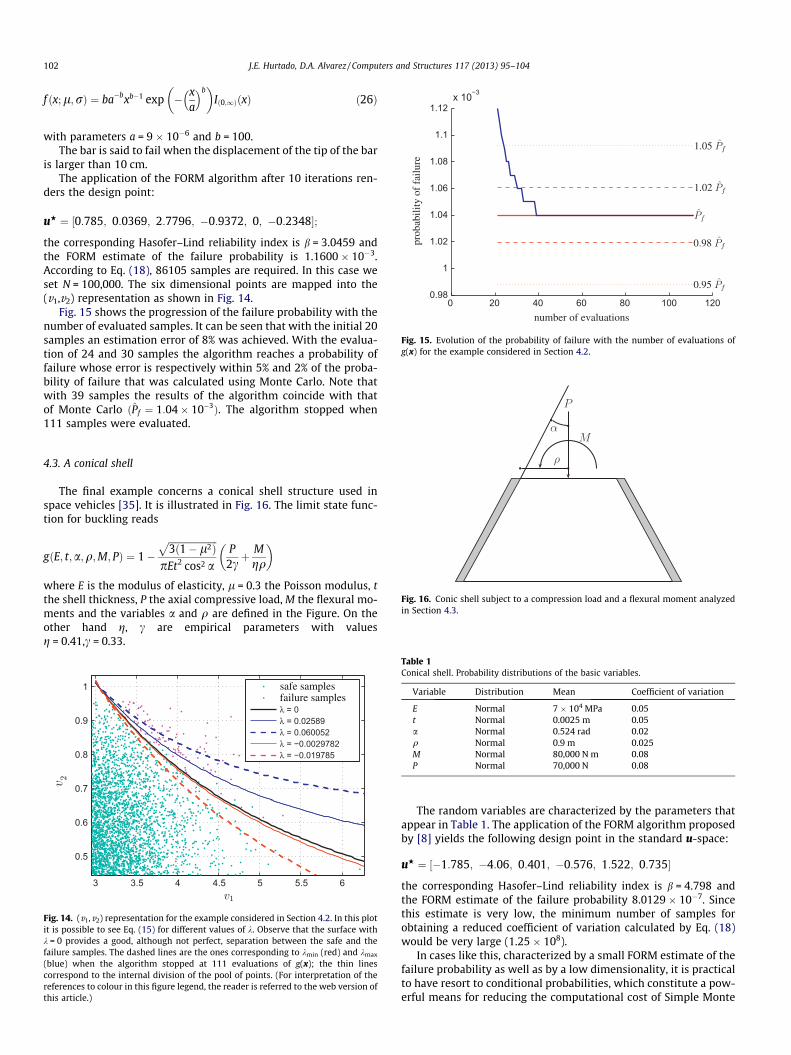
Fig. 15. Evolution of the probability of failure with the number of evaluations ofg(x) for the example considered in Section 4.2.

102 J.E. Hurtado, D.A. Alvarez / Computers and Structures 117 (2013) 95–104

f ðx; l;rÞ ¼ ba�bxb�1 exp � xa

� b� �

Ið0;1ÞðxÞ ð26Þ

with parameters a = 9 � 10�6 and b = 100.The bar is said to fail when the displacement of the tip of the bar

is larger than 10 cm.The application of the FORM algorithm after 10 iterations ren-

ders the design point:

uH ¼ ½0:785; 0:0369; 2:7796; �0:9372; 0; �0:2348�;

the corresponding Hasofer–Lind reliability index is b = 3.0459 andthe FORM estimate of the failure probability is 1.1600 � 10�3.According to Eq. (18), 86105 samples are required. In this case weset N = 100,000. The six dimensional points are mapped into the(v1,v2) representation as shown in Fig. 14.

Fig. 15 shows the progression of the failure probability with thenumber of evaluated samples. It can be seen that with the initial 20samples an estimation error of 8% was achieved. With the evalua-tion of 24 and 30 samples the algorithm reaches a probability offailure whose error is respectively within 5% and 2% of the proba-bility of failure that was calculated using Monte Carlo. Note thatwith 39 samples the results of the algorithm coincide with thatof Monte Carlo ðPf ¼ 1:04� 10�3Þ. The algorithm stopped when111 samples were evaluated.

Fig. 16. Conic shell subject to a compression load and a flexural moment analyzedin Section 4.3.

4.3. A conical shell

The final example concerns a conical shell structure used inspace vehicles [35]. It is illustrated in Fig. 16. The limit state func-tion for buckling reads

gðE; t;a;q;M; PÞ ¼ 1�ffiffiffiffiffiffiffiffiffiffiffiffiffiffiffiffiffiffiffiffiffi3ð1� l2Þ

ppEt2 cos2 a

P2cþ M

gq

� �

where E is the modulus of elasticity, l = 0.3 the Poisson modulus, tthe shell thickness, P the axial compressive load, M the flexural mo-ments and the variables a and q are defined in the Figure. On theother hand g, c are empirical parameters with valuesg = 0.41,c = 0.33.

3 3.5 4 4.5 5 5.5 6

0.5

0.6

0.7

0.8

0.9

1

λ = 0λ = 0.02589λ = 0.060052λ = −0.0029782λ = −0.019785

safe samplesfailure samples

Fig. 14. (v1,v2) representation for the example considered in Section 4.2. In this plotit is possible to see Eq. (15) for different values of k. Observe that the surface withk = 0 provides a good, although not perfect, separation between the safe and thefailure samples. The dashed lines are the ones corresponding to kmin (red) and kmax

(blue) when the algorithm stopped at 111 evaluations of g(x); the thin linescorrespond to the internal division of the pool of points. (For interpretation of thereferences to colour in this figure legend, the reader is referred to the web version ofthis article.)

Table 1Conical shell. Probability distributions of the basic variables.

Variable Distribution Mean Coefficient of variation

E Normal 7 � 104 MPa 0.05t Normal 0.0025 m 0.05a Normal 0.524 rad 0.02q Normal 0.9 m 0.025M Normal 80,000 N m 0.08P Normal 70,000 N 0.08

The random variables are characterized by the parameters thatappear in Table 1. The application of the FORM algorithm proposedby [8] yields the following design point in the standard u-space:

uH ¼ ½�1:785; �4:06; 0:401; �0:576; 1:522; 0:735�

the corresponding Hasofer–Lind reliability index is b = 4.798 andthe FORM estimate of the failure probability 8.0129 � 10�7. Sincethis estimate is very low, the minimum number of samples forobtaining a reduced coefficient of variation calculated by Eq. (18)would be very large (1.25 � 108).

In cases like this, characterized by a small FORM estimate of thefailure probability as well as by a low dimensionality, it is practicalto have resort to conditional probabilities, which constitute a pow-erful means for reducing the computational cost of Simple Monte

J.E. Hurtado, D.A. Alvarez / Computers and Structures 117 (2013) 95–104 103

Carlo simulation, as in the Subset Simulation [36] and Radial-basedImportance Sampling methods [37,38]. In these latter, the failureprobability computed in the standard Normal space u is exactly gi-ven by

Pf ¼ Pf jxPx ð27Þ

Here Pfjx is the probability of failure given that the norm of variableu is greater than x, where x is the radius of any hypersphere lyingentirely in the safe domain:

Pf jx ¼ P½gðuÞ 6 0 j kuk > x� ð28Þ

This term is estimated by Monte Carlo simulation with samples ly-ing strictly beyond the hypersphere of radius x. On the other hand,the second factor in Eq. (27) is given by

Px ¼ P½kuk > x� ¼ 1� v2ðx2; dÞ ð29Þ

where v2(x2,d) is the chi-square distribution calculated at x2 withd degrees of freedom.

Evidently, in applying this procedure the value of x must belower than b for assuring that all failure samples will be identifiedby the proposed algorithm. On the other hand, the coefficient ofvariation in Eq. (17) should be computed over the estimate of Pfjx,because it is the factor evaluated by Monte Carlo simulation. Thus,the number of samples for building the plot was obtained as

N > 1001� Pf jx

Pf jx¼ 98;562

because Pf jx ¼ 8:0129�10�7

1�v2ð4:7982 ;6Þ¼ 0:001. Thus, the plot was created with

N = 100,000 standard Gaussian samples generated beyond a hyper-sphere of radius x = 4.5 < b. Therefore, Px = 0.0025. The results ofthe computation are shown in Fig. 17. The number of function eval-uations is 22, which is a very small number indeed. The total num-ber of failure samples is composed by 22 found in the selectedsector plus 15 above the kmax = 0.003364 line. The failure probabil-ity estimate is, therefore, 3.7 � 10�4 � 0.0025 = 9.2477 � 10�7,which coincides with the Monte Carlo result, because all failuresamples were correctly detected once again.

4.5 5 5.5 6 6.5 7−1

−0.8

−0.6

−0.4

−0.2

0

0.2

0.4

0.6

0.8

1

λ = 0λ = 0.0041885λ = 0.03364λ = −0.01689λ = −0.028586

safe samplesfailure samples

Fig. 17. Results of the application of the proposed approach to the shell problemanalyzed in Section 4.3. The dashed lines are the ones corresponding to kmin (red)and kmax (blue) when the algorithm stopped at 22 evaluations of g(x); the thin linescorrespond to the internal division of the pool of points. (For interpretation of thereferences to colour in this figure legend, the reader is referred to the web version ofthis article.)

5. Conclusions

A method for structural reliability analysis has been presented.The method is intended to improve the estimates given by theFirst-Order Reliability Method (FORM), not only because it is themost popular method in this field but, more importantly, becausethe design point vector possesses significant clustering properties.They allow visual discrimination of the safe and failure classes ofMonte Carlo samples in a bi-dimensional plot constituted by twononlinear features extracted from the realizations of the input ran-dom variables. In addition the plot has also a standard form inwhich the failure samples naturally accommodate in its upper-right sector. This standard enormously facilitates the selection ofthe highly relevant samples for reliability analysis from the plot,that also proves to be very robust with respect to the dimensional-ity of the problem. An algorithm for computing the failure proba-bility based on the second-order expansion of the limit statefunction was proposed. Its application with some practical struc-tural cases demonstrates the high accuracy, low computationalcost and practical appeal of the method, as it allows visualizationof the reliability analysis as a whole.

Acknowledgement

Financial support for the realization of the present research hasbeen received from the Universidad Nacional de Colombia. Thesupport is graciously acknowledged.

References

[1] Nataf A. Determination des distributions dont les marges sont donées. CR AcadSci 1962;225:42–3.

[2] Liu PL, Der Kiureghian A. Multivariate distribution models with prescribedmarginals and covariances. Probab Eng Mech 1986;1:105–12.

[3] Winterstein SR. Nonlinear vibration modes for extremes and fatigue. J EngMech 1988;114:1772–90.

[4] Ditlevsen O, Madsen HO. Structural reliability methods. Chichester: John Wileyand Sons; 1996.

[5] Madsen HO, Krenk S, Lind NC. Methods of structural safety. New York: DoverPublications; 2006.

[6] Hasofer AM, Lind NC. Exact and invariant second moment code format. J EngMech Div 1974;100:111–21.

[7] Rackwitz R, Fiessler B. Structural reliability under combined load sequences.Comput Struct 1978;9:489–94.

[8] Liu PL, Der Kiureghian A. Optimization algorithms for structural reliability.Struct Saf 1991;9:161–77.

[9] Lemaire M. Structural reliability. New York: ISTE–Wiley; 2009.[10] Zhao YG, Ono T. A general procedure for first/second-order reliability method

(FORM/SORM). Struct Saf 1999;21:955–1112.[11] Ditlevsen O. Generalized second moment reliability index. J Struct Mech

1979;7:435–51.[12] Schuëller GI, Stix R. A critical appraisal of methods to determine failure

probabilities. Struct Saf 1987;4:293–309.[13] Zhao YG, Ono T. New approximations for SORM: Part I. J Eng Mech

1999;125:79–85.[14] Mahadevan S, Shi P. Multiple linearization method for nonlinear reliability

analysis. J Eng Mech 2001;127:1165–73.[15] Eamon CD, Thompson M, Liu Z. Evaluation of accuracy and efficiency of some

simulation and sampling methods in structural reliability analysis. Struct Saf2005;27:356–92.

[16] Valdebenito MA, Pradlwarter HJ, Schuëller GI. The role of the design point forcalculating failure probabilities in view of dimensionality and structuralnonlinearities. Struct Saf 2010;21:101–11.

[17] Katafygiotis LS, Zuev KM. Geometric insight into the challenges of solvinghigh-dimensional reliability problems. Probab Eng Mech 2008;23:208–18.

[18] Au SK, Beck JL. Importance sampling in high dimensions. Struct Saf2003;25:139–63.

[19] Der Kiureghian A. The geometry of random vibrations and solutions by FORMand SORM. Probab Eng Mech 2000;15:81–90.

[20] Koo H, Der Kiureghian A, Fujimura K. Design-point excitation for non-linearrandom vibrations. Probab Eng Mech 2005;20:136–47.

[21] Fujimura K, Der Kiureghian A. Tail-equivalent linearization method fornonlinear random vibration. Probab Eng Mech 2007;22:63–76.

[22] Benjamin JR, Cornell CA. Probability, statistics and decision for civilengineers. New York: McGraw-Hill; 1970.

[23] Rubinstein RY. Monte Carlo optimization, simulation and sensitivity ofqueuing networks. Malabar: Krieger Publishing Company; 1992.

104 J.E. Hurtado, D.A. Alvarez / Computers and Structures 117 (2013) 95–104

[24] Fiessler B, Neumann HJ, Rackwitz R. Quadratic limit states in structuralreliability. J Eng Mech Div 1979;105:661–76.

[25] Tvedt L. Distribution of quadratic forms in normal space – application tostructural reliability. J Eng Mech 1990;116:1183–7.

[26] Breitung K. Asymptotic approximation for multinormal integrals. J Eng Mech1984;110:357–66.

[27] Der Kiureghian A, Lin HZ, Hwang SJ. Second-order reliability approximations. JEng Mech 1987;113:1208–25.

[28] Der Kiureghian A, Di Stefano M. Efficient algorithm for second-order reliabilityanalysis. J Eng Mech 1991;117:2904–23.

[29] Cai GQ, Elishakoff I. Refined second-order reliability analysis. Struct Saf1994;14:267–76.

[30] Choi SK, Grandhi RV, Canfield RA. Reliability-based structuraldesign. London: Springer; 2010.

[31] Zhao YG, Ono T. New approximations for SORM: Part II. J Eng Mech1999;125:86–93.

[32] Shooman ML. Probabilistic reliability: an engineering approach. NewYork: McGraw-Hill; 1968.

[33] Ohsaki M, Ikeda K. Stability and optimization of structures. NewYork: Springer; 2010.

[34] McGuire W, Gallagher RH, Ziemian RD. Matrix structural analysis. 2nd ed. NewYork: John Wiley and Sons; 2000.

[35] Elegbede C. Structural reliability assessment based on particle swarmoptimization. Struct Saf 2005;27:171–86.

[36] Au SK, Beck JL. Estimation of small failure probabilites in high dimensions bysubset simulation. Probab Eng Mech 2001;16:263–77.

[37] Harbitz A. An efficient sampling method for probability of failure calculation.Struct Saf 1986;3:109–15.

[38] Grooteman F. Adaptive radial-based importance sampling method forstructural reliability. Struct Saf 2008;30:533–42.