sensors

Article

A Method for Detecting Atmospheric LagrangianCoherent Structures Using a Single Fixed-WingUnmanned Aircraft System

Peter J. Nolan 1,* , Hunter G. McClelland 2, Craig A. Woolsey 2 and Shane D. Ross 1

1 Engineering Mechanics Program, Virginia Tech, Blacksburg, VA 24061, USA; sdross@vt.edu2 Kevin T. Crofton Department of Aerospace and Ocean Engineering, Virginia Tech,

Blacksburg, VA 24061, USA; hgm@vt.edu (H.G.M.); cwoolsey@vt.edu (C.A.W.)* Correspondence: pnolan86@vt.edu; Tel.: +1-540-231-1616

Received: 14 February 2019; Accepted: 27 March 2019; Published: 3 April 2019�����������������

Abstract: The transport of material through the atmosphere is an issue with wide ranging implicationsfor fields as diverse as agriculture, aviation, and human health. Due to the unsteady nature of theatmosphere, predicting how material will be transported via the Earth’s wind field is challenging.Lagrangian diagnostics, such as Lagrangian coherent structures (LCSs), have been used to discoverthe most significant regions of material collection or dispersion. However, Lagrangian diagnosticscan be time-consuming to calculate and often rely on weather forecasts that may not be completelyaccurate. Recently, Eulerian diagnostics have been developed which can provide indications of LCSand have computational advantages over their Lagrangian counterparts. In this paper, a methodologyis developed for estimating local Eulerian diagnostics from wind velocity data measured by a singlefixed-wing unmanned aircraft system (UAS) flying in a circular arc. Using a simulation environment,driven by realistic atmospheric velocity data from the North American Mesoscale (NAM) model, it isshown that the Eulerian diagnostic estimates from UAS measurements approximate the true localEulerian diagnostics and also predict the passage of LCSs. This methodology requires only a singleflying UAS, making it easier and more affordable to implement in the field than existing alternatives,such as multiple UASs and Dopler LiDAR measurements. Our method is general enough to beapplied to calculate the gradient of any scalar field.

Keywords: unmanned aircraft system (UAS); Lagrangian coherent structure (LCS); atmospherictransport

1. Introduction

The transport of material in the atmosphere is a problem with important implications foragriculture [1–4], aviation [5,6], and human health [7,8]. Given the unsteady nature of atmosphericflows, it can be difficult to predict where a fluid parcel, such as one containing an airborne pathogen,will be transported. Tools from dynamical systems theory, such as Lagrangian coherent structures(LCSs), can help us to understand how fluid parcels in a flow will evolve. The study of atmospherictransport from a dynamical systems perspective has long focused on the study of large-scalephenomena [1–5,9–12]. This has been largely due to the larger-scale grid spacing of readily availableatmospheric model data and the lack of high-resolution atmospheric measurements on a scale largeenough to calculate Lagrangian data. Furthermore, this field of study has been largely relegatedto numerical simulations. Few works have attempted to find ways to directly detect LCSs fromexperimental measurements in the field. In [6,13], the authors used wind velocity measurements froma Doppler light detection and ranging (LiDAR) to detect LCS which had passed near Hong Kong

Sensors 2019, 19, 1607; doi:10.3390/s19071607 www.mdpi.com/journal/sensors

Sensors 2019, 19, 1607 2 of 21

International Airport. Rather than measure the wind velocity to try to detect LCSs, the authors of [1]looked at sudden changes in pathogen concentrations in the atmosphere. They were then able tolink those changes to the passage of LCSs using atmospheric velocity data from the North AmericanMesoscale (NAM) weather research and forecasting (WRF) model. Recent advances in dynamicalsystems theory, such as new Eulerian diagnostics, as well as new atmospheric sensing technology,such as unmanned aircraft systems (UAS) [14], have brought the local detection of LCSs within thereach of operators in the field at any location, without the need for expensive infrastructure. Onerecent paper took advantage of these new advances to attempt to predict the passage of LCSs based onexperimental data. The authors of [15] used multiple sonic anemometers attached to two stationaryairborne quadcopter UASs and one ground-based tower to measure the wind velocity around theSan Luis Valley in Colorado. From these wind measurements, the authors were able to calculate thelocal attraction rate, which was then compared to the attraction rate from a WRF simulation. Fromthese comparisons, the authors found indicators of LCSs associated with convective cells and a frontwhich passed through the region. In this paper, we build upon these recent developments to establisha method to detect LCSs which can be readily implemented by operators in the field at any location,using only a single fixed-wing UAS.

The first of these developments is new Eulerian techniques for measuring the attraction andrepulsion of regions in a fluid flow [16,17]. In traditional Lagrangian analyses, a velocity field isneeded, which is defined over a large enough spatiotemporal scale to allow the accurate simulationof fluid parcel trajectories. How the parcels are transported by the flow is then used to determinewhich parts of the flow are more attractive or repulsive. These new Eulerian methods do not rely onthe simulation of fluid parcel trajectories; instead, they are based on the instantaneous gradients ofthe velocity field. Since they rely on gradients, these techniques only require enough velocity datapoints to enact a finite-differencing scheme. Furthermore, these methods are Eulerian and can thus beapplied to data sets which are temporally coarse.

The second of these developments is the use of inexpensive UASs to sample the atmosphericvelocity instead of piloted aircraft or other traditional assets. Ground-based wind sensors such asLiDAR, sonic detection and ranging (SoDAR), or tower-mounted anemometers can be prohibitivelyexpensive and difficult to relocate in real time to regions of interest, such as a chemical release, wildfire, or radioactive release. Airborne wind measurement from aircraft has a long history [18,19] andwell-developed existing programs, such as the NASA Airborne Science Program [20]. The advancementof UASs has enabled wind measurement missions which may be of lower cost, longer duration, andcan be implemented in more dangerous environments. Elston et al. [21] provided a review of manyUAS atmospheric measurement efforts, and recent works continue to advance both theoretical andpractical UAS capabilities [22–27].

This paper develops a methodology which will enable researchers in the field to utilize local windmeasurements to detect LCSs using only a single UAS. This methodology will be less complex, lessexpensive, and less time-consuming to implement than those utilized in previous studies [1,6,13,15].Furthermore, by requiring only a single fixed-wing UAS, the need for expensive infrastructure andmultiple pilot/spotter teams is eliminated. Additionally, since this methodology takes advantage ofEulerian diagnostics, there is no need for expensive computer clusters or time-consuming trajectoryintegration, as with Lagrangian diagnostics. This methodology is developed and tested using anobserving system simulation experiment (OSSE). A historical wind velocity forecast from the NAMmodel is taken and passed to a UAS flight simulator, which is assumed to have a perfect anemometer,but still includes the effects of the wind field on the aircraft’s flight trajectory. The simulated UASattempts to fly in a circular orbit about a portion of the NAM model centered on the coordinatesof the Virginia Tech experimental site, Kentland Farm, Figure 1. From wind measurements alongthese circular orbits, we were able to calculate the local trajectory divergence rate and attraction rate,described in Section 2.1. Using these calculations, it is then possible to look for signals of LCSs passingthrough the area.

Sensors 2019, 19, 1607 3 of 21

This paper is organized as follows. Section 2.1 describes the Eulerian and Lagrangian diagnosticswhich are used to analyze the atmospheric velocity data. Section 2.2 describes the algorithm wedevelop to calculate the gradient of a scalar field from measurements along a circular arc, which isnecessary for the computation of the Eulerian diagnostics. Section 2.3 briefly describes the NAMmodel which is used, how the model data are prepared for analysis, and the flight simulator which isused. In Section 3.1, the results of a parametric study which analyzes the ability of a UAS flying in acircular arc to approximate Eulerian diagnostics over various radii are presented. Section 3.2 presentsresults concerning the ability of Eulerian diagnostics to approximate Lagrangian diagnostics anddetect LCSs passing through an area using receiver operating characteristic (ROC) curves. Due to thediscrete nature of numerical computations, a parametric study to investigate various area thresholdsfor the detection of LCSs was performed. Section 3.3 presents results concerning the ability of Euleriandiagnostics, as approximated from a simulated UAS flight, to detect LCSs passing through an area.Once again, a parametric study to investigate various area thresholds for the detection of LCSs usingROC curves is performed. Section 4 discusses the results presented in Section 3. Finally, Section 5presents the conclusion of the paper.

Kentland Farm

Figure 1. Map of the Mid-Atlantic United States, Kentland Farm in Virginia is shown in red.

2. Methods

2.1. Lagrangian-Eulerian Analysis

Consider the dynamical system:

ddt

x(t) = v(x(t), t), (1)

x0 = x(t0), (2)

x(t) ∈R2, t ∈ R, (3)

where x(t) is the position vector of a fluid parcel at time t and v(x, t) is the time-varying horizontalwind velocity vector at position x(t) and time t. The components of the horizontal position vector arex = (x, y), where x is the eastward position and y is the northward position, and the horizontal velocityvector, v = (u, v), where u is the eastward velocity and v is the northward velocity. This system canbe analyzed using both Langrangian and Eulerian tools. For the Lagrangian analysis, the finite-time

Sensors 2019, 19, 1607 4 of 21

Lyapunov exponent (FTLE), σ, and Lagrangian coherent structures (LCSs) are used. For this study,LCSs are defined as C-ridges of the FTLE field following [28]. The FTLE field is a measure ofthe stretching of fluid parcels within a flow, the forward-time FTLE measures repulsion, and thebackward-time FTLE measures attraction. LCSs are the most attracting and repelling material surfaceswithin a fluid flow; as such, they provide a means of visualizing how particles within the flow willevolve. For the Eulerian analyses, the attraction rate, s1, and the trajectory divergence rate, ρ, are used.Both of these rates are derived from the Eulerian rate-of-strain tensor, S, described below. The attractionrate is the minimum eigenvalue of S and was shown in [16] to provide a measure of instantaneoushyperbolic attraction, with isolated minima of s1 providing the cores of attracting objective Euleriancoherent structures (OECS). Recent work has shown that in 2D, s1 is the limit of the backward-timeFTLE as the integration time goes to 0 and that troughs of s1 are attracting infinitesimal-time LCS(iLCS) [29], a schematic of which can be seen in Figure 2. The trajectory divergence rate is a measureof how much repulsion/attraction is changing along streamlines of the velocity field, as depicted inFigure 3 [17].

Fluid parcel

Trough of

s1

Figure 2. Schematic of the effect of a trough of the attraction rate, s1, field on a fluid parcel.

Figure 3. Schematic of the trajectory divergence rate: Where ρ < 0, trajectories are instantaneouslyconverging; where ρ > 0 trajectories are instantaneously diverging.

To calculate the Lagrangian metrics, first calculate the flow map of the vector field (1) for the timeperiod of interest:

Ftt0(x0) = x0 +

∫ t

t0

v(x(t), t) dt. (4)

Taking the gradient of the flow map, the right Cauchy–Green strain tensor is then calculated:

Ctt0(x0) = ∇Ft

t0(x0)

T · ∇Ftt0(x0), (5)

with ordered eigenvalues, λ1 ≤ λ2. From the largest eigenvalue of the right Cauchy–Green straintensor, λ2, the FTLE field is derived:

σtt0(x0) =

12|t− t0|

log (λ2(x0)) . (6)

Ridges of this field can then be identified as LCSs.

Sensors 2019, 19, 1607 5 of 21

For the Eulerian metrics, the Eulerian rate-of-strain tensor is defined as:

S(x0, t0) =12

(∇v(x0, t0) +∇v(x0, t0)

T)

, (7)

with ordered eigenvalues s1 ≤ s2. The attraction rate is defined as the minimum eigenvalue of S, s1.The attraction rate can be directly calculated from the velocity gradient using the formula:

s1 = 12

(∂u∂x + ∂v

∂y

)− 1

2

√(∂u∂x −

∂v∂y

)2+(

∂u∂y + ∂v

∂x

)2. (8)

The trajectory divergence rate is defined wherever v(x0, t0) 6= 0 as:

ρ(x0, t0) = n(x0, t0)T · S(x0, t0) · n(x0, t0) =

(v(x0, t0)

T · JT · S(x0, t0) · J · v(x0, t0))

||v(x0, t0)||2, (9)

where n(x0, t0) is the unit vector normal to the trajectory and J is the matrix, J =[ 0 1−1 0

][17].

2.2. Gradient Approximation from UAS Flight

In order to calculate the Eulerian rate-of-strain tensor from wind measurements along a simulatedUAS flight path, we developed an algorithm to approximate the gradient of a scalar field based onmeasurements along a circular arc, Figure 4. The algorithm is based on a quasi-frozen field assumptionthat the scalar field is not significantly changing in time during the period of one full orbit but ischanging in space. We believe this assumption is appropriate to apply to atmospheric velocity fields,as mid- to larger-scale atmospheric flows tend to change on the order of hours, while UAS orbitson the spatial scale of interest are on the order of minutes. This assumption of course ignores smallscale turbulent motion, which would fall below the scale which is being sampled. This algorithm alsoassumes that the important features will be in the horizontal plane. This assumption was previouslyapplied to atmospheric model data in [9,10,30] and atmospheric measurements in [15]. It is based onthe fact that the vertical component of the wind velocity tends to be two orders of magnitude less thanthe horizontal components. We assume that the inertial velocity of the aircraft, V , and the air-relativevelocity, Vr, are independently measured, using, for instance, GPS-based instruments, orientationinformation from a gyroscope, and a pitot tube anemometer. The wind velocity is v = V − Vr.See Appendix A for further details.

Figure 4. Schematic showing positions where velocity measurements were made and the position ofthe circle gradient frame to the reference frame.

Sensors 2019, 19, 1607 6 of 21

We remark that while we developed the algorithm described below for measurements of thegradient of the horizontal wind velocity components, u and v, the algorithm is general enough to beapplied to the gradient of any scalar value, f , measured by a UAS, such as air temperature, pressure,and humidity.

This algorithm takes as inputs:

• A scalar field measured along a circular arc, f (θ), as an n× 1 array input, where n is the numberof measurements taken;

• The angle θ as a monotonically decreasing n× 1 array input;• And the radius of the circular arc, r, which is assumed to be constant, as a scalar input.

Note, this algorithm is currently written for a clockwise trajectory. The algorithm starts withan initial point along the circular arc (r, θ0) and the value f at that point. Then, provided the pathcontinues for at least another three quarters of a circle, the value of f is obtained at three additionalpoints along the path at (r, θ0 − 1

2 π), (r, θ0 − π), and (r, θ0 − 32 π). With f at four individual points

along the circular arc, a central finite-difference scheme is used to approximate the gradient of f atthe center point of the circle. Since the four points are along an arc, each subsequent approximationthe gradient will be in a reference frame which has a different orientation from the initial gradientapproximation, Figure 4. To correct for this, apply a counterclockwise rotation to the gradient of f toobtain the gradient in a consistent reference frame oriented North–South, East–West. Continue foreach additional point along the circular arc until there is less than an additional three quarters of acircle left. A pseudo-code version of this algorithm can be found in Algorithm 1, and a schematic canbe found in Figure 4.

Algorithm 1 CIRCLE GRADIENT approximates the gradient of a scalar from samples along an arcInput: r, θ, f (θ)Output: Approximation of ∇ f

1 for i← 1 to length(θ) do2 if θ(i)− 3

2 π ≥ θ(end) then3 Obtain f (θ) at f (θ(i)) , f

(θ(i)− 1

2 π)

, f (θ(i)− π) , f(θ(i)− 3

2 π)

4∂ f∂x′ ≈

f (θ(i))− f (θ(i)−π)2·r

5∂ f∂y′ ≈

f (θ(i)− 32 π)− f (θ(i)− 1

2 π)2·r

6 ∇ f (i) ≈[

cos(θ(i)) sin(θ(i))− sin(θ(i)) cos(θ(i))

] [ ∂ f∂x′∂ f∂y′

]7 return ∇ f

2.3. Model Data

For the OSSE, velocity field data from the 3 km NAM model [31] were utilized. This velocity fieldwas from the portion of the model over southwestern Virginia and was centered at the Virginia Techexperimental site, Kentland Farm (Figure 1), during a 215 h period beginning 4 September 2017 at00:00 UTC. The NAM data were divided into 2 data sets. The first part was a strictly 2D data set thatwas restricted to the 850 mb isosurface. The second was a 3D data set. Both data sets were interpolatedin time from 1 h resolution down to 10 min resolution using cubic splines. The 3D data were theninterpolated from pressure-based vertical levels to height above sea level (ASL) vertical levels usinglinear interpolation. Both data sets were also interpolated from a 3 km horizontal resolution to a 300 mhorizontal resolution using cubic Lagrange polynomials. An aircraft was simulated using closed-looptrajectory control to fly fixed-radius circles. These circles varied in radius from 2 km to 15 km. Smallerradii, more consistent with the federal regulations in FAA part 107 (i.e., to keep aircraft within unaidedsight) [32], were examined; however, the simulated wind velocity field, with a grid resolution of 3 km,

Sensors 2019, 19, 1607 7 of 21

lacked the spatial inhomogeneity necessary to compute meaningful gradients below a 2 km flightradius (4 km flight diameter). The simulated aircraft was also set to track the 850 mb isosurface withthe 3D wind velocity field acting as a disturbance. The altitude of the 850 mb isosurface varies in time;it is approximately at 1545 m ASL. A subscale model of a transport-style aircraft, named the T-2 [33],was used as the simulated unmanned aircraft. To get a sense of the aircraft’s scale, some of its physicalproperties are:

mass m = 22.5 kg, wingspan b = 2.09 m, chord c = 0.28 m, airspeed ||Vr|| ≈ 42 m/s.

With the T-2’s cruising airspeed of approximately 42 m/s, a full orbit takes between 300 to 2250 s,depending on the orbit radius. For a comparison, the average horizontal wind speed of the NAMmodel at the 850 mb isosurface was approximately 10 m/s. The details of the flight dynamic modelare included in Appendix A. The simulated wind measurements taken by the aircraft are wind fieldcomponents v along the aircraft’s center-of-mass trajectory x(t). Figure 5 shows several orbits duringthe aircraft’s flight. Note that the vertical dimension is scaled to be 500 times bigger than the horizontal,in order to show flight path differences between consecutive orbits.

radius

Figure 5. Simulated 3D unmanned aircraft systems (UAS) flight path (solid blue line) along with a 2Dperfect circle (dotted black line). The 2D circle is at a constant altitude, while the 3D UAS flight tracksthe 850 mb isosurface. The vertical dimension is shown highly exaggerated.

3. Results

3.1. Approximating Local Eulerian Metrics from UAS Flights

This section presents results which indicate how well the attraction rate, s1, and the trajectorydivergence rate, ρ, can be approximated from a UAS flight. Figure 6 shows the results for the trajectorydivergence rate. From the 2D velocity field, restricted to the 850 mb isosurface, measurements alongperfectly circular paths, with radii fixed between 2 km and 15 km, were used to approximate thetrajectory divergence rate, shown in black. Then, velocity measurements from 3D simulated UASflight paths with radii fixed between 2 km and 15 km, attempting to follow the 850 mb isosurface,were used to approximate the trajectory divergence rate, shown in blue. Finally, using the 850 mbisosurface velocity field, the true trajectory divergence rate at the center point of the circle/flight radius

Sensors 2019, 19, 1607 8 of 21

was calculated, shown in red. Pearson correlation coefficients for these measurements can be foundin Table 1.

Figure 7 shows the results for the attraction rate. As before, using measurements along perfectlycircular paths, with radii fixed between 2 km and 15 km, from a 2D velocity field restricted to the850 mb isosurface, the attraction rate was approximated, shown in black. Then, the attraction ratewas approximated using velocity measurements from 3D simulated UAS flight paths, with radii fixedbetween 2 km and 15 km, attempting to follow the 850 mb isosurface, shown in blue. Finally, using the850 mb isosurface velocity field, the true attraction rate at the center point of the circle/flight radiuswas calculated, shown in red. Pearson correlation coefficients for these measurements can be found inTable 2.

−1

0

1

hr−

1

2km 5km

True ρ flight circle

50 100 150 200

Hours

−1

0

1

hr−

1

10km

50 100 150 200

Hours

15km

Figure 6. Comparison of measurements of the trajectory divergence rate ρ at the center point of thecircular sampling orbit (red), along the path of a simulated UAS flight (black), and along a circular arc(blue). The radius of the circle and flight path is shown in the lower right hand corner of each subplot.The circular arc and the simulated UAS flight are nearly on top of each other.

Table 1. Pearson correlation coefficients for trajectory divergence rate, ρ, measurements. Coefficientsrange from 0.730 to 0.965.

2 km Circle 5 km Circle 10 km Circle 15 km Circle 2 km Flight 5 km Flight 10 km Flight 15 km Flight

center point 0.955 0.854 0.790 0.730 0.931 0.827 0.781 0.7302 km circle -- 0.946 0.815 0.751 0.981 0.923 0.811 0.7655 km circle -- 0.866 0.768 0.935 0.981 0.865 0.784

10 km circle -- 0.928 0.804 0.836 0.974 0.90215 km circle -- 0.745 0.738 0.904 0.9552 km flight -- 0.944 0.824 0.7835 km flight -- 0.870 0.79310 km flight -- 0.937

Sensors 2019, 19, 1607 9 of 21

Table 2. Pearson correlation coefficients for attraction rate, s1, measurements. Coefficients range from0.577 to 0.939.

2 km Circle 5 km Circle 10 km Circle 15 km Circle 2 km Flight 5 km Flight 10 km Flight 15 km Flight

center point 0.939 0.838 0.677 0.590 0.910 0.821 0.675 0.5772 km circle -- 0.932 0.742 0.644 0.980 0.917 0.739 0.6275 km circle -- 0.898 0.789 0.916 0.980 0.887 0.760

10 km circle -- 0.908 0.729 0.881 0.978 0.86415 km circle -- 0.637 0.788 0.907 0.9652 km flight -- 0.936 0.746 0.6445 km flight -- 0.900 0.79110 km flight -- 0.909

−2

−1

0

1

hr−

1

2km 5km

True s1 flight circle

50 100 150 200

Hours

−2

−1

0

1

hr−

1

10km

50 100 150 200

Hours

15km

Figure 7. Comparison of measurements of the attraction rate s1 at the center point of the circularsampling orbit (red), along the path of a simulated UAS flight (black), and along a circular arc (blue).The radius of the circle and flight path is shown in the lower right hand corner of each subplot.The circular arc and the simulated UAS flight are nearly on top of each other.

3.2. Using Eulerian Metrics to Infer Lagrangian Dynamics

In this section, results which indicate how well the attraction rate, s1, and the trajectory divergencerate, ρ, predicts Lagrangian dynamics, such as the passage of LCSs, are presented. Figure 8 shows thetime series for the trajectory divergence rate and backward-time FTLE for integration times of 0.5, 1,and 2 h. Figure 9 shows the time series for the attraction rate and backward-time FTLE for integrationtimes of 0.5, 1, and 2 h. The FTLE values have been multiplied by −1 for improved visualization.These values were calculated using velocity data from the 850 mb isosurface over the Kentland Farmportion of the NAM model.

The effectiveness of the attraction rate and the trajectory divergence rate for detecting LCSs wasfurther explored using receiver operating characteristic (ROC) curves. ROC curves plots the truepositive rate against the false positive rate for different threshold levels. Figure 10 shows an example of

Sensors 2019, 19, 1607 10 of 21

a true positive and a false positive from this study. To define these curves, we determined when LCSspassed within a threshold radius which ranged from 400 m to 10 km of the center point, Figure 11.We further applied a threshold of 90% for the LCSs, so only LCSs whose FTLE value was above the90th percentile were considered. The attraction rate’s and the trajectory divergence rate’s ability todetect LCSs for integration times of 0.5, 1, and 2 h in backward-time was explored. Figure 12 shows anidealized ROC curve with different threshold values; the farther the ROC curve is from the dotted line,the better the sensor is. This can be quantified using the area under the curve (AUC). The larger theAUC is above 0.5, the better the sensor is; a perfect sensor would have an AUC of 1.

25 50 75 100 125 150 175 200

Hours

−2.0

−1.5

−1.0

−0.5

0.0

0.5

1.0

hr−

1

ρ

σ, T=0.5hr

σ, T=1hr

σ, T=2hr

Figure 8. Comparison of the trajectory divergence rate with the 0.5, 1, and 2 h backward-time finite-timeLyapunov exponent (FTLE) from t = 4 to t = 215 h. FTLE fields have been multiplied by −1 to offerbetter comparison of attraction.

25 50 75 100 125 150 175 200

Hours

−2.0

−1.5

−1.0

−0.5

0.0

0.5

1.0

hr−

1

s1

σ, T=0.5hr

σ, T=1hr

σ, T=2hr

Figure 9. Comparison of the attraction rate with the 0.5, 1, and 2 h backward-time FTLE from t = 4 tot = 215 h. FTLE fields have been multiplied by −1 to offer better comparison of attraction.

Sensors 2019, 19, 1607 11 of 21

Figure 13 shows ROC curves for the the trajectory divergence rate as measured from the centerpoint of the sampling area (Figure 11). The threshold ranges from 0% at the upper right hand corner to100% at the lower left hand corner. Every 20th percentile is marked with a dot. Each subplot representsa different threshold radius, with radii ranging from 400 m to 10 km. Each color represents a differentintegration time for the LCSs, 0.5 h green, 1 h red, 2 h blue. The AUC ranges from 0.477 to 0.756.

Figure 10. Depiction of a true positive (left) and a false positive (right), from approximately 43.5 h and20.67 h, respectively. The true attraction rate field over Kentland Farm Va. is displayed; darker greensare lower values of the attraction rate. Grid points where the value of the attraction rate is above thethreshold value are masked (white). Attracting LCS with an integration time of −1 h are shown asblue lines. The threshold radius is shown by the black dashed circle and has a radius of 5 km. In bothexamples, the attraction rate at the center of the sampling domain is below the threshold value, thusmeeting the criterion for a positive identification of an LCS passing within the threshold radius. In thetrue positive example, there is an LCS passing within the threshold radius. Meanwhile, in the falsepositive, there is no LCS within the threshold radius. The ROC plot point for the particular case shownin this figure (i.e., threshold value and 5.0 km radius) is depicted by a red “+" marker in Figure 14.

7.5 km threshold radius

2.0 km UAS flight

0.8 km threshold radius

Center point

Attracting LCS

Figure 11. Schematic of Lagrangian coherent structure (LCS) detection showing two examples ofthreshold radii as dashed lines. An attracting LCS falls within the larger threshold radius but does notfall within the smaller radius. The instantaneous wind field is depicted as the background vector field.

Sensors 2019, 19, 1607 12 of 21

0.0 0.2 0.4 0.6 0.8 1.0

False Positive Rate

0.0

0.2

0.4

0.6

0.8

1.0

TruePositiveRate

100%

80%

60% 40% 20% 0%

Figure 12. Schematic of an idealized receiver operating characteristic (ROC) curve and with threshold percentiles.

0.00

0.25

0.50

0.75

1.00 0.4km

0.706

0.609

0.611

0.8km

0.707

0.756

0.621

0.5hr 1hr 2hr

1.2km

0.695

0.721

0.588

0.00

0.25

0.50

0.75

1.00

TruePositiveRate

1.6km

0.685

0.700

0.600

2.0km

0.638

0.684

0.586

3.0km

0.598

0.647

0.522

0.0 0.5 1.0

0.00

0.25

0.50

0.75

1.00 5.0km

0.577

0.578

0.477

0.0 0.5 1.0

False Positive Rate

7.5km

0.598

0.555

0.491

0.0 0.5 1.0

10.0km

0.551

0.530

0.485

Figure 13. ROC curves for the trajectory divergence rate, ρ, as measured at the center point ability todetect 90th percentile LCSs with integration times of 0.5 (green), 1 (red), and 2 (blue) h. Thresholdradius for each subplot is displayed in the upper left hand corner. The area under the curve (AUC) foreach integration time is given in the legend.

Sensors 2019, 19, 1607 13 of 21

Figure 14 shows ROC curves for the attraction rate as measured from the center point of thesampling area (Figure 11). As before, the threshold is applied to the attraction rate ranging from 0%,upper right hand corner, to 100%, lower left hand corner. Every 20th percentile is marked with a dot.Each subplot represents a different threshold radius, with radii ranging from 400 m to 10 km. Eachcolor represents a different integration time for the LCSs, 0.5 h green, 1 h red, 2 h blue. The AUCranges from 0.626 to 0.850.

0.00

0.25

0.50

0.75

1.00 0.4km

0.849

0.732

0.751

0.8km

0.850

0.806

0.734

0.5hr 1hr 2hr

1.2km

0.845

0.808

0.735

0.00

0.25

0.50

0.75

1.00

TruePositiveRate

1.6km

0.841

0.811

0.734

2.0km

0.840

0.805

0.709

3.0km

0.834

0.811

0.682

0.0 0.5 1.0

0.00

0.25

0.50

0.75

1.00 5.0km

0.803

0.806

0.666

0.0 0.5 1.0

False Positive Rate

7.5km

0.736

0.711

0.647

0.0 0.5 1.0

10.0km

0.682

0.662

0.626

Figure 14. ROC curves for the attraction rate, s1, as measured at the center point ability to detect 90thpercentile LCSs with integration times of 0.5 (green), 1 (red), and 2 (blue) h. The threshold radius foreach subplot is displayed in the upper left hand corner. The AUC for each integration time is given inthe legend. The red “+” marker corresponds to the plot point for the case (i.e., threshold value andradius) that was shown in Figure 10.

3.3. Inferring Lagrangian Dynamics from UAS Measurements

This section presents results which indicate how well the attraction rate, s1, and the trajectorydivergence rate, ρ, as approximated from a simulated UAS flight, predict Lagrangian dynamics, suchas the passage of LCSs, Figure 11. Figure 15 shows ROC curves for the the trajectory divergencerate as calculated from a simulated 2 km radius UAS flight. The threshold ranges from 0% at theupper right hand corner to 100% at the lower left hand corner. Every 20th percentile is marked witha dot. Each subplot represents a different threshold radius, with radii ranging from 400 m to 10 km.Each color represents a different integration time for the LCSs, 0.5 h green, 1 h red, 2 h blue. The AUCranges from 0.491 to 0.742.

Sensors 2019, 19, 1607 14 of 21

0.00

0.25

0.50

0.75

1.00 0.4km

0.698

0.596

0.633

0.8km

0.684

0.742

0.632

0.5hr 1hr 2hr

1.2km

0.675

0.717

0.605

0.00

0.25

0.50

0.75

1.00

TruePositiveRate

1.6km

0.668

0.697

0.618

2.0km

0.635

0.678

0.601

3.0km

0.598

0.644

0.543

0.0 0.5 1.0

0.00

0.25

0.50

0.75

1.00 5.0km

0.582

0.581

0.499

0.0 0.5 1.0

False Positive Rate

7.5km

0.609

0.558

0.499

0.0 0.5 1.0

10.0km

0.562

0.533

0.491

Figure 15. ROC curves for the trajectory divergence rate, ρ, as measured from a 2 km radius UASsimulation ability to detect 90th percentile LCSs with integration times of 0.5 (green), 1 (red), and2 (blue) h. The threshold radius for each subplot is displayed in the upper left hand corner. The AUCfor each integration time is given in the legend.

Figure 16 shows ROC curves for the attraction rate as calculated from a simulated 2 km UASflight. As before, the threshold is applied to the attraction rate ranging from 0%, upper right handcorner, to 100%, lower left hand corner. Every 20th percentile is marked with a dot. Each subplotrepresents a different threshold radius, with radii ranging from 400 m to 10 km. Each color representsa different integration time for the LCSs, 0.5 h green, 1 h red, 2 h blue. The AUC ranges from 0.602to 0.874.

Sensors 2019, 19, 1607 15 of 21

0.00

0.25

0.50

0.75

1.00 0.4km

0.874

0.607

0.736

0.8km

0.835

0.753

0.746

0.5hr 1hr 2hr

1.2km

0.843

0.764

0.767

0.00

0.25

0.50

0.75

1.00

TruePositiveRate

1.6km

0.856

0.770

0.772

2.0km

0.846

0.778

0.752

3.0km

0.821

0.778

0.714

0.0 0.5 1.0

0.00

0.25

0.50

0.75

1.00 5.0km

0.775

0.767

0.673

0.0 0.5 1.0

False Positive Rate

7.5km

0.725

0.698

0.635

0.0 0.5 1.0

10.0km

0.656

0.647

0.602

Figure 16. ROC curves for the attraction rate, s1, as measured from a 2 km radius UAS simulationability to detect 90th percentile LCSs with integration times of 0.5 (green), 1 (red), and 2 (blue) h.The threshold radius for each subplot is displayed in the upper left hand corner. The AUC for eachintegration time is given in the legend.

4. Discussion

Looking at the results in Figure 6, we can see that the simulated UAS flight in 3D space providesa very similar result to the circular path restricted to the 850 mb isosurface. For all the radii that wereanalyzed, the trajectory divergence rate from the flight simulation is nearly identical to that from theidealized 2D circular path. Most of the error between the center point trajectory divergence rate andthe estimate from the 3D flights appears to be due to the distance from the point of estimation, ratherthan inconsistencies in the flight’s path due to the UAS being buffeted by wind. This can also be seenin Table 1, where the correlation coefficients between the simulated flight and the 2D circle are all >0.95,while there is a steady drop in the correlation coefficients with the center point trajectory divergencerate as the radius increases.

Looking at the results in Figure 7, we see that the simulated UAS flight in 3D space provides verysimilar attraction rate measurements to the circular path restricted to the 850 mb isosurface. As before,for all the radii paths that were examined, the attraction rate from the flight simulation is nearlyidentical to that from the 2D circular path. Most of the error between the center point attraction rateand the estimate from the 3D flights appears to be due to the distance from the point of estimation,rather than inconsistencies in the flight’s path due to the UAS being buffeted by wind. This can also beseen in Table 2, where the correlation coefficients between the simulated flight and the 2D circle are

Sensors 2019, 19, 1607 16 of 21

all >0.96, while there is a steep drop in the correlation coefficients with the center point attraction rateas the radius increases.

Both the attraction rate and the trajectory divergence rate at a point can be approximated to a highdegree of accuracy by UAS flights. Simulated 3D UAS flights provided measurements which werenearly identical to those of perfect circular 2D paths. The main cause of error in the approximationsappears to be the radius of the circular arc. Furthermore, the trajectory divergence rate appears to be amore robust metric than the attraction rate, meaning that the trajectory divergence rate can be betterapproximated at larger radii than the attraction rate can. This can be seen very clearly in Tables 1 and 2,where the correlation coefficient for the attraction rate drops off more quickly with flight radius thanfor the trajectory divergence rate.

As mentioned previously, the smallest flight radius which was explored in this study was 2 km.This radius was chosen because under 2 km, the spatial inhomogeneity of the simulated velocity fieldwas insufficient to compute meaningful gradients. However, under current federal regulations in FAApart 107, unaided visual contact must be maintained with the UAS [32]. For smaller UASs, it is unlikelythat an operator would be able to satisfy this requirement at a flight radius of 2 km. Fortunately,these results suggest that as the flight radius is decreased, the UAS approximation of the Euleriandiagnostic will converge the true value at the center point. Thus, we anticipate that in real-worldexperiments, where the flight radius will be on the order of hundreds of meters, a single fixed-wingUAS will provide an accurate approximation to the Eulerian diagnostics at the center point.

Figure 8 shows that the trajectory divergence rate does not always follow the trend of the negativebackward-time FTLE. This is to be expected, as the trajectory divergence rate gives information on bothinstantaneous attraction and repulsion, while the negative backward-time FTLE gives only a measureof attraction. The trajectory divergence rate does, however, agree with the negative backward-timeFTLE during periods of significant (large) attraction. This behavior is of particular interest for thedetection of LCSs. When calculating LCSs, there is often a multitude of weaker, less important LCSs.In order to filter out these less important structures and focus on important structures, one often needsto set a threshold value for the FTLE field. These dips in the the trajectory divergence rate, coincidingwith the strongest dips in the negative backward-time FTLE, would therefore seem to be a likelyindicator of the most influential LCSs.

Figure 9 shows that the attraction rate follows the general trend of the negative backward-timeFTLE. This is consistent as both the attraction rate and the negative backward-time FTLE give measuresof attraction. The attraction rate appears to give a good approximation to the negative backward-timeFTLE, and thus should be able to give indications of LCSs.

The ROC curves in Figure 13 show that the trajectory divergence rate, calculated at a point, canbe used to detect the passage of LCSs. For the smaller threshold radii, AUC values for the ROC curvesgreater than 0.6 are consistently seen. This means that this method is outperforming random guessing,which would have an AUC of 0.5. Of course, as the threshold radius increases, the AUC trends to0.5. This convergence to random chance at larger thresholds is consistent, since as the sample areaincreases, the likelihood of an LCS being within that domain will converge to 100%, at least for realisticatmospheric flows.

The ROC curves in Figure 14 show that the attraction rate, calculated at a point, cannot only beused to detect the passage of LCSs, but that it performs better at LCS detection than the trajectorydivergence rate does. The smaller and more moderate threshold radii consistently display AUC valuesfor the ROC curves of greater than 0.7, and many well over 0.8. This means that this method is faroutperforming random guessing. Once again, it can be seen that as the threshold radius increases,the AUC trends towards 0.5, although this convergence is happening slower than it did with thetrajectory divergence rate.

It should be noted that both the attraction and trajectory divergence rates seem to perform best ata threshold radius of around 0.8–2.0 km and become noisier as the radius decreases. We suspect thatthis is due to the spatial and temporal scales of the input data, 3 km × 1 h grid spacing. We speculate

Sensors 2019, 19, 1607 17 of 21

that with a velocity field that is either analytically defined or more highly resolved in both space andtime, continued improvement in the ROC curves as the threshold radius decreases would be seen.Unfortunately, the analytical models currently used in the study of LCSs in 2D, such as the doublegyre [34] and the Bickley jet [35], do not have the requisite spatial inhomogeneity necessary to revealmeaningful Eulerian structures in the attraction rate or the trajectory divergence rate fields.

The ROC curves in Figure 15 show that the trajectory divergence rate, as calculated from asimulated 2 km UAS flight, can be used to detect the passage of LCSs. For the smaller, and evenmore moderate, threshold radii, AUC values for the ROC curves greater than 0.6 are consistently seen.This means that this method is outperforming random guessing. Of course, as the threshold radiusincreases, the AUC trends to 0.5.

The ROC curves in Figure 16 show that the attraction rate, as calculated from a simulated 2 kmUAS flight, cannot only be used to detect the passage of LCSs but once again performs better at LCSdetection than the trajectory divergence rate does. For the smaller and more moderate threshold,radii consistently display AUC values for the ROC curves greater than 0.7, and many well over 0.8.This means that this method is outperforming random guessing. Once again, as the threshold radiusincreases, the AUC trends towards 0.5, although this convergence is happening slower than it did withthe trajectory divergence rate.

In this paper, a planar circular flight path was used to determine if it is possible to detect an LCSpassing through a given domain. However, this is just one potential application. More complicatedflight paths could, hypothetically, be used to determine the size and shape of an LCS. For example,a corkscrew trajectory could potentially be used to determine the height of an LCS; likewise, a spiralingtrajectory could potentially be used to determine the length of an LCS, or even to track an LCS asit moves.

The UAS-related results presented above were all calculated using Algorithm 1. Algorithm 1assumes that the input scalar field is accurately measured and changing smoothly in time. In reality,experimental wind measurements are expected to have non-negligible error, both noise and bias types.It is still an open question as to how sensor error will affect these results. Future work will explore towhat extent this LCS detection methodology is robust to that error.

5. Conclusions

We have put forward a novel algorithm to approximate the gradient of a scalar field usingmeasurements from a circular arc around a point. Using realistic atmospheric velocity data from theNAM 3 km model, this algorithm was applied to circular trajectories restricted to a 2D isosurfaceand simulated UAS flights in 3D, with radii ranging from 2 km to 15 km. From these results, thetrajectory divergence rate and the attraction rate were approximated for the center point of thesepaths. Comparing these approximations with the true trajectory divergence rate and attraction rate atthe center point, we found that both the realistic flight simulator and the circle give nearly identicalapproximations. Furthermore, the approximations were very good for the smaller radii that werelooked at, but even the larger radii approximations were able to pick up the trend of the trajectorydivergence rate and attraction rate, though they underestimated the magnitude.

We have also examined the ability of Eulerian diagnostics, in particular the trajectory divergenceand attraction rates, to infer Lagrangian dynamics. Using ROC curves, the ability of the trajectorydivergence rate and attraction rate, as calculated at a point, to detect the passage of LCSs within athreshold radius was explored. We found that the attraction rate can be used as an effective tool todetect short term LCSs passing by. We also found that the trajectory divergence rate, while performingbetter than chance, underperformed the attraction rate. This analysis was then extended to look at thetrajectory divergence rate and attraction rate as approximated by a UAS flight. Once again, we foundthat these Eulerian diagnostics, as approximated by a UAS flight, can be an effective tool for detectingLCSs passing through a sampling area.

Sensors 2019, 19, 1607 18 of 21

This paper serves as a first step towards in situ detection of LCSs in the atmosphere. It demonstratesthat a single fixed-wing UAS can, in principle, be used to measure Eulerian diagnostics of a localatmospheric flow. These Eulerian diagnostics can then be used to infer the Lagrangian dynamics of thelocal flow. Future work will apply this paper’s techniques to experimental data to detect real-worldatmospheric LCSs using a fixed-wing UAS, evaluate the effects of sensor uncertainty on the accuracyof LCS detection, examine additional flight paths to attempt to determine size and shape of LCS,and extend the analysis to the detection of pollutant specific LCSs [5,12,36].

Author Contributions: Conceptualization, P.J.N. and H.G.M. and C.A.W. and S.D.R.; methodology, P.J.N. andH.G.M. and C.A.W. and S.D.R.; investigation, P.J.N. and H.G.M.; writing—original draft preparation, P.J.N.;writing—review and editing, P.J.N. and H.G.M.; visualization, P.J.N. and H.G.M.; supervision, S.D.R. and C.A.W.;funding acquisition, H.G.M. and S.D.R. and C.A.W.

Funding: This research was supported in part by grants from the National Science Foundation (NSF) undergrant numbers AGS 1520825 (Hazards SEES: Advanced Lagrangian Methods for Prediction, Mitigation andResponse to Environmental Flow Hazards) and DMS 1821145 (Data-Driven Computation of Lagrangian TransportStructure in Realistic Flows) and the National Aeronautics and Space Administration (NASA) under grant number80NSSC17K0375 (NASA Earth and Space Science Fellowship). Any opinions, findings, and conclusions orrecommendations expressed in this material are those of the authors and do not necessarily reflect the views ofthe sponsors.

Acknowledgments: We thank Javier González-Rocha, Gary K. Nave, and David G. Schmale for fruitful discussionsduring the writing of this paper.

Conflicts of Interest: The authors declare no conflict of interest.

Abbreviations

The following abbreviations are used in this manuscript:

UAS Unmanned aircraft systemsASL Above sea levelAUC Area under the curveFTLE Finite-time Lyapunov exponentLCS Lagrangian coherent structureiLCS Infinitesimal-time LCSOECS Objective Eulerian coherent structureWRF Weather research and forecastingNAM North American Mesoscale modelOSSE Observing system simulation experimentROC Receiver Operating Characteristic

Appendix A. Flight Dynamic Model

The aircraft flight dynamic model is derived by combining standard aircraft rigid-bodyequations [37] with Grauer and Morelli’s Generic Global Aerodynamic model [33], modified fornon-uniform wind. The important flight dynamic modeling assumptions are:

1. Earth is a flat, inertial reference.2. The aircraft is a rigid body, symmetric about its longitudinal plane, with constant mass m.3. For wind-aircraft interaction, the aircraft is a point “located” at it’s center-of-mass.4. The wind is described by a C1-smooth kinematic vector field.5. Aircraft thrust fth is an instantaneously-controllable force acting nose-forward from the center-of-mass.6. All parameters are invariant with altitude. (e.g., no altitudinal variation of density ρ, gravity g,

ground-effect, etc.)

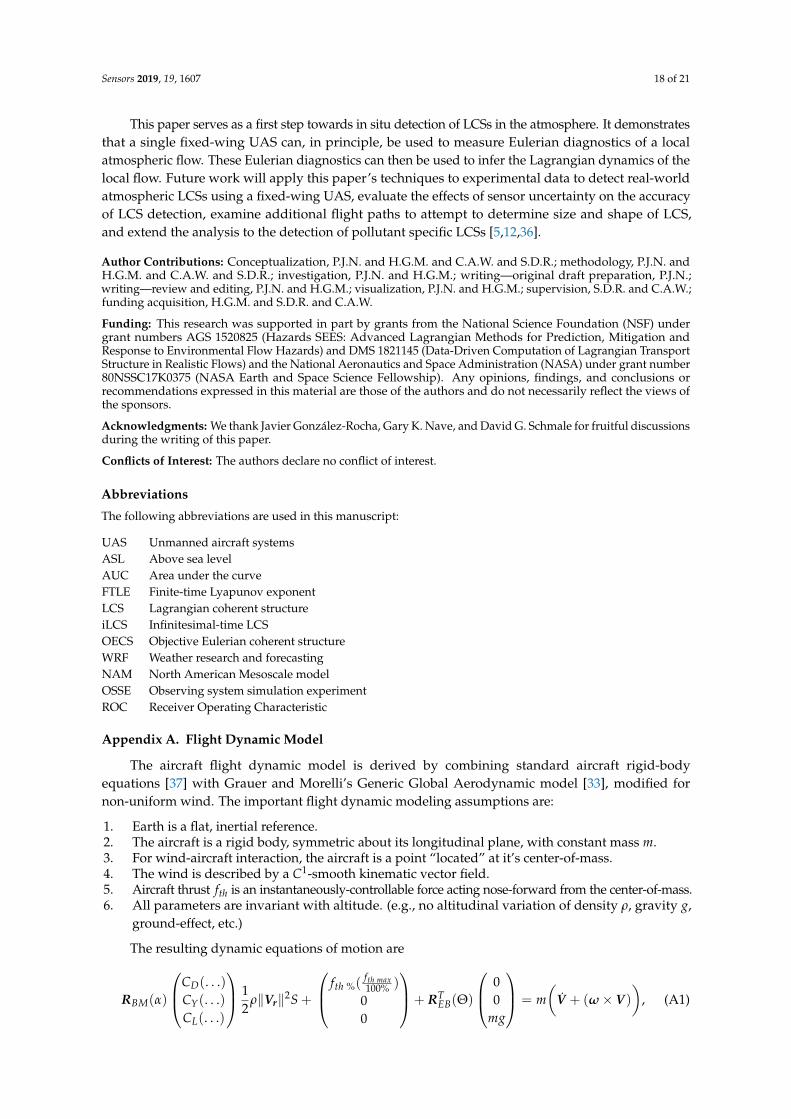
The resulting dynamic equations of motion are

RBM(α)

CD(. . .)CY(. . .)CL(. . .)

12

ρ‖Vr‖2S +

fth %( fth max100% )

00

+ RTEB(Θ)

00

mg

= m(

V + (ω× V)

), (A1)

Sensors 2019, 19, 1607 19 of 21

b 0 00 c 00 0 b

Cl(. . .)

Cm(. . .)Cn(. . .)

12

ρ‖Vr‖2S =

Ixx 0 −Ixz

0 Iyy 0−Ixz 0 Izz

ω +(

ω×

Ixx 0 −Ixz

0 Iyy 0−Ixz 0 Izz

ω)

. (A2)

where the ellipses on the aerodynamic coefficients remind the reader that these are functions of statevariables, as given below in (A5)–(A10). The symbol V is used for inertially-referenced velocity, andVr is used for air-relative velocity. Thus, V = Vr + v, where v is the wind vector from the atmosphericsimulation described in Section 2.3. The notation RBM(α) represents the rotation matrix, which dependson the angle-of-attack α, from the aircraft’s body-frame to the modified-stability frame in which Grauerand Morelli’s aerodynamic forces are defined. Similarly, REB(Θ) is the rotation matrix from the Earthframe to the aircraft’s body frame. The rest of the notation is in agreement with Etkin [37]. Thesedynamics are combined with standard translational and rotational kinematic equations

X = REB(φ, θ, ψ)

UVW

= REB(Θ)V , (A3)

Θ =

φ

θ

ψ

=

1 sin φ tan θ cos φ tan θ

0 cos φ − sin φ

0 sin φ sec θ cos φ sec θ

p

qr

= L−1(φ, θ)ω. (A4)

The aerodynamic coefficient expressions are from Equation (20) of Grauer and Morelli [33],

CD = θ1 + θ2α + θ3αqr + θ4αδe + θ5α2 + θ6α2qr + θ7α2δe + θ8α3 + θ9α3qr + θ10α4, (A5)

CY = θ11β + θ12 pr + θ13rr + θ14δa + θ14δr, (A6)

CL = θ16 + θ17α + θ18qr + θ19δe + θ20αqr + θ21α2 + θ22α3 + θ23α4, (A7)

Cl = θ24β + θ25 pr + θ26rr + θ27δa + θ28δr, (A8)

Cm = θ29 + θ30α + θ31qr + θ32δe + θ33αqr + θ34α2qr + θ35α2δe + θ36α3qr + θ37α3δe + θ38α4, (A9)

Cn = θ39β + θ40 pr + θ41rr + θ42δa + θ43δr + θ44β2 + θ45β3. (A10)

In these equations, (θ1, θ2, . . . θ45) are the aircraft parameters specific to the T-2 aircraft assumedin this study, described in Section 2.3. In addition, (α, β) are the standard aerodynamic angles,( pr, qr, rr) are wind-relative non-dimensionalized angular rates, and (δa, δe, δr) are aileron, elevator,and rudder deflections.

References

1. Tallapragada, P.; Ross, S.D.; Schmale, D.G. Lagrangian Coherent Structures Are Associated with Fluctuationsin Airborne Microbial Populations. Chaos 2011, 21, 033122. [CrossRef] [PubMed]

2. Schmale, D.; Ross, S. Highways in the Sky: Scales of Atmospheric Transport of Plant Pathogens.Annu. Rev. Phytopathol. 2015, 53, 591–611. [CrossRef] [PubMed]

3. Schmale, D.G.; Ross, S.D. High-flying microbes: Aerial drones and chaos theory help researchers explore themany ways that microorganisms spread havoc around the world. Sci. Am. 2017, 2, 32–37.

4. BozorgMagham, A.E.; Ross, S.D.; Schmale, D.G., III. Local finite-time Lyapunov exponent, local samplingand probabilistic source and destination regions. Nonlinear Process. Geophys. 2015, 22, 663–677. [CrossRef]

5. Peng, J.; Peterson, R. Attracting structures in volcanic ash transport. Atmos. Environ. 2012, 48, 230–239.[CrossRef]

6. Tang, W.; Chan, P.W.; Haller, G. Lagrangian coherent structure analysis of terminal winds detected by lidar.Part I: Turbulence structures. J. Appl. Meteorol. Climatol. 2011, 50, 325–338. [CrossRef]

7. Kampa, M.; Castanas, E. Human health effects of air pollution. Environ. Pollut. 2008, 151, 362–367. [CrossRef][PubMed]

Sensors 2019, 19, 1607 20 of 21

8. Pope, C., III; Burnett, R.T.; Thun, M.J.; Calle, E.E.; Krewski, D.; Ito, K.; Thurston, G.D. Lung cancer, cardiopulmonarymortality, and long-term exposure to fine particulate air pollution. JAMA 2002, 287, 1132–1141. [CrossRef][PubMed]

9. BozorgMagham, A.E.; Ross, S.D. Atmospheric Lagrangian coherent structures considering unresolvedturbulence and forecast uncertainty. Commun. Nonlinear Sci. Numer. Simul. 2015, 22, 964–979. [CrossRef]

10. Senatore, C.; Ross, S.D. Detection and characterization of transport barriers in complex flows via ridgeextraction of the finite time Lyapunov exponent field. Int. J. Numer. Methods Eng. 2011, 86, 1163–1174.[CrossRef]

11. Curbelo, J.; García-Garrido, V.J.; Mechoso, C.R.; Mancho, A.M.; Wiggins, S.; Niang, C. Insights into thethree-dimensional Lagrangian geometry of the Antarctic polar vortex. Nonlinear Process. Geophys. 2017, 24, 379.[CrossRef]

12. Garaboa-Paz, D.; Eiras-Barca, J.; Huhn, F.; Pérez-Muñuzuri, V. Lagrangian coherent structures alongatmospheric rivers. Chaos Interdiscip. J. Nonlinear Sci. 2015, 25, 063105. [CrossRef]

13. Knutson, B.; Tang, W.; Chan, P.W. Lagrangian coherent structure analysis of terminal winds: Three-dimensionality,intramodel variations, and flight analyses. Adv. Meteorol. 2015, 2015. [CrossRef]

14. González-Rocha, J.; Woolsey, C.A.; Sultan, C.; De Wekker, S.F. Sensing Wind from Quadrotor Motion. J. Guid.Control Dyn. 2018. doi:10.2514/1.G003542. [CrossRef]

15. Nolan, P.; Pinto, J.; González-Rocha, J.; Jensen, A.; Vezzi, C.; Bailey, S.; de Boer, G.; Diehl, C.; Laurence, R.;Powers, C.; et al. Coordinated Unmanned Aircraft System (UAS) and Ground-Based Weather Measurementsto Predict Lagrangian Coherent Structures (LCSs). Sensors 2018, 18, 4448. [CrossRef]

16. Serra, M.; Haller, G. Objective Eulerian coherent structures. Chaos: Interdiscip. J. Nonlinear Sci. 2016, 26, 053110.[CrossRef]

17. Nave, G.K., Jr.; Nolan, P.J.; Ross, S.D. Trajectory-free approximation of phase space structures using thetrajectory divergence rate. Nonlinear Dyn. 2019. doi:10.1007/s11071-019-04814-z. [CrossRef]

18. Axford, D.N. On the Accuracy of Wind Measurements Using an Inertial Platform in an Aircraft, and anExample of a Measurement of the Vertical Mesostructure of the Atmosphere. J. Appl. Meteorol. Climatol.1968, 7, 645–666. [CrossRef]

19. Lenschow, D.H.; Spyers-Duran, P. Measurement Techniques: Air Motion Sensing; Technical Report 23; NationalCenter for Atmospheric Research: Boulder, CO, USA, 1989.

20. NASA. Airborne Science Program Website. Available online: https://airbornescience.nasa.gov/ (accessedon 31 January 2017).

21. Elston, J.; Argrow, B.; Stachura, M.; Weibel, D.; Lawrence, D.; Pope, D. Overview of Small Fixed-WingUnmanned Aircraft for Meteorological Sampling. J. Atmos. Ocean. Technol. 2015, 32, 97–115. [CrossRef]

22. Borup, K.T.; Fossen, T.I.; Johansen, T.A. A Nonlinear Model-Based Wind Velocity Observer for UnmannedAerial Vehicles. In Proceedings of the 10th IFAC Symposium on Nonlinear Control Systems, Monterey, CA,USA, 23–25 August 2016.

23. Rhudy, M.B.; Gu, Y.; Gross, J.N.; Chao, H. Onboard Wind Velocity Estimation Comparison for UnmannedAircraft Systems. IEEE Trans. Aerosp. Electron. Syst. 2017, 53, 55–66. [CrossRef]

24. Lie, F.A.P.; Gebre-Egziabher, D. Synthetic Air Data System. J. Aircr. 2013, 50, 1234–1249. [CrossRef]25. Langelaan, J.W.; Alley, N.; Neidhoefer, J. Wind Field Estimation for Small Unmanned aerial Vehicles. J. Guid.

Control Dyn. 2011, 34, 1016–1030. [CrossRef]26. Witte, B.M.; Singler, R.F.; Bailey, S.C. Development of an Unmanned Aerial Vehicle for the Measurement of

Turbulence in the Atmospheric Boundary Layer. Atmosphere 2017, 8, 195. [CrossRef]27. Wenz, A.; Johansen, T.A. Estimation of Wind Velocities and Aerodynamic Coefficients for UAVs using

Standard Autopilot Sensors and a Moving Horizon Estimator. In Proceedings of the IEEE InternationalConference on Unmanned Aircraft Systems (ICUAS), Miami, FL, USA, 13–16 June 2017; pp. 1267–1276.

28. Peikert, R.; Schindler, B.; Carnecky, R. Ridge surface methods for the visualization of Lagrangiancoherent structures. In Proceedings of the 9th International Conference on Flow Dynamics, Sendai, Japan,19–21 September 2012; pp. 206–207.

29. Nolan, P.J.; Ross, S.D. Finite-time Lyapunov exponent field in the infinitesimal time limit. viXra 2018,viXra:1810.0023.

Sensors 2019, 19, 1607 21 of 21

30. BozorgMagham, A.E.; Ross, S.D.; Schmale, D.G., III Real-time prediction of atmospheric Lagrangiancoherent structures based on forecast data: An application and error analysis. Phys. D Nonlinear Phenom.2013, 258, 47–60. [CrossRef]

31. North American Mesoscale Model. Available online: https://www.emc.ncep.noaa.gov/NAM/.php.(accessed on 18 January 2019).

32. Fact Sheet – Small Unmanned Aircraft Regulations (Part 107). Available online: https://www.faa.gov/news/fact_sheets/news_story.cfm?newsId=22615. (accessed on 8 March 2019).

33. Grauer, J.A.; Morelli, E.A. Generic Global Aerodynamic Model for Aircraft. J. Aircr. 2015, 52, 13–21.[CrossRef]

34. Shadden, S.C.; Lekien, F.; Marsden, J.E. Definition and properties of Lagrangian coherent structuresfrom finite-time Lyapunov exponents in two-dimensional aperiodic flows. Phys. D Nonlinear Phenom.2005, 212, 271–304. [CrossRef]

35. Rypina, I.; Brown, M.; Beron-Vera, F.; Kocak, H.; Olascoaga, M.; Udovydchenkov, I. On the Lagrangiandynamics of atmospheric zonal jets and the permeability of the stratospheric polar vortex. J. Atmos. Sci.2007, 64, 3595–3610. [CrossRef]

36. Nolan, P.J.; Foroutan, H.; Ross, S.D. The Understanding of Pollutant Transport in the Atmosphere:Lagrangian Coherent Structures. Poster Presented by Hosein Foroutan at the 17th Annual CMAS Conference,2018. Available online: https://cmascenter.org/conference//2018/slides/foroutan_understanding_pollutant_2018.pdf (accessed on 3 March 2019).

37. Etkin, B. Dynamics of Atmospheric Flight; John Wiley & Sons: New York, NY, USA, 1972.

c© 2019 by the authors. Licensee MDPI, Basel, Switzerland. This article is an open accessarticle distributed under the terms and conditions of the Creative Commons Attribution(CC BY) license (http://creativecommons.org/licenses/by/4.0/).