A MCMC Analysis of Time-Changed Levy Processes ofStock Return Dynamics

HAITAO LIa, MARTIN WELLSb, and LONG YUc

April, 2004

Preliminary and for comments only

aLi is from Johnson Graduate School of Management, Cornell University, Ithaca, NY 14853. bMartin Wells is from

the Department of Statistical Sciences, Cornell University, Ithaca, NY 14853. cLong Yu is from the Department of

Statistical Sciences, Cornell University, Ithaca, NY 14853. We would like to thank Torben Andersen and Luca Benzoni

for providing the data used in the early stage of this study. We are responsible for any remaining errors.

A MCMC Analysis of Time-Changed Levy Processes of Stock Return Dynamics

ABSTRACT

We provide a Bayesian analysis of a time-changed Levy process model of stock return dynamics us-

ing Markov Chain Monte Carlo (MCMC) methods. Our models exhibit stochastic volatility through

a random time change and Levy jumps. In contrast to the widely used finite-activity compound

Poisson processes, the infinite-activity Levy jumps here allow for an infinite number of jumps within

any finite time interval. Therefore, Levy processes are better suited to capture highly frequent dis-

continuous movements in the stock prices. Estimation of Levy processes can be challenging, because

for certain models, such as the α-stable process, the probability density is not known in closed-form

and higher moments of asset returns do not exist. We develop MCMC techniques that have excel-

lent performance in estimating model parameters, latent stochastic volatility, and jump variables of

time-changed Levy processes. Empirically, we demonstrate that for the S&P 500 index, models with

stochastic volatility and Levy jumps in returns significantly outperform those with Poisson jumps

in both returns and volatility. In fact, once Levy jumps in returns are included, Poisson jumps in

stochastic volatility become much less important.

1 Introduction

Despite the enormous success of the Black and Scholes (1973) and Merton (1973) option pricing

model, it is widely recognized that the model cannot fully capture some important features of stock

return data. From a time series perspective, there is strong evidence that stock returns exhibit

conditional heteroskedasticity and large discontinuous jumps, even though the model assumes that

stock price follows a continuous process with constant volatility. From a cross-sectional perspective,

the Black-Scholes-Merton model systematically misprices options across moneyness and maturity.

The well-known volatility smile or skew strongly indicates that the underlying asset returns do not

follow a normal distribution.1 Motivated by the apparent shortcomings of the Black-Scholes-Merton

model, a huge literature has been developed in the past few decades to search for better models of

stock returns.

A major part of the literature focuses on models that belong to the so-called affine jump-diffusions

(hereafter AJDs) of Duffie, Pan, and Singleton (2000), in which stock prices are driven by affine

diffusion and compound Poisson process.2 One of the main reasons for the popularity of AJDs is

their tractability. As shown by Duffie, Pan, and Singleton (2000), Chacko and Das (2001), and

others, AJDs allow closed-form solutions for a wide range of equity and fixed-income derivatives.

Classical AJDs for equity returns include: (i) the jump-diffusion model of Merton (1976), which

assumes that stock prices exhibit both continuous, diffusive movements modeled by Brownian motion,

and large, discontinuous jumps, modeled by Poisson process; (ii) the stochastic volatility model of

Heston (1993), which allows stock return volatility itself to follow a separate diffusion process. More

sophisticated models with both stochastic volatility and jumps have also been developed.

The empirical performance of AJDs of stock returns has been extensively studied using either

stock or option data, or both.3 For example, Bates (1996, 2000) and Bakshi, Cao and Chen (1997)

provide comprehensive analyses of stochastic volatility and jump models using option data. Chernov

and Ghysels (2002) and Pan (2002) estimate stochastic volatility and jump models using both option

and stock data jointly. On the other hand, Andersen, Benzoni, and Lund (2002) examine models

1See Rubinstein (1994) and many related studies on volatility smile/skew in the options market.2In AJDs, the drift and diffusion terms of the diffusion part of the model are linear functions of the underlying state

variables, and the intensity of the compound Possion process is also a linear function of the state variables.3The literature is too large to be thoroughly reviewed here. In our following discussion, we will only focus on those

studies that are most closely related to our paper.

1

with stochastic volatility and compound Poisson jumps using underlying S&P 500 index returns. The

existing evidence provides support for AJDs and show that any reasonable model should exhibit a

stochastic volatility that is strongly negatively correlated with return process as well as large discrete

jumps.

However, Bates (2000), Duffie, Pan, and Singleton (2000), and Pan (2002) show that AJDs are still

misspecified for major U.S. stock market indexes. Specifically, they show that the volatility variables

tend to rapidly increase, which is difficult to reconcile with a stochastic volatility that follows a

diffusion process. Recently, Eraker, Johannes, and Polson (2003) (hereafter EJP) show that jumps

in both returns and volatility process are needed to capture the dynamics of S&P 500 and Nasdaq

100 index returns. Specifically, allowing jumps in stochastic volatility captures the rapid increase

in volatility process and significantly improves model performance. Chernov, Gallant, Ghysels, and

Tauchen (2003) also show that models with two stochastic volatility factors, one highly persistent

and another rapidly moving, have similar performance as models with jumps in both returns and

volatility. Eraker (2003) provides supporting evidence of jumps in both returns and volatility using

spot and option prices jointly.

While AJDs significantly improve the Black-Scholes-Merton model, they still have certain limita-

tions. For example, compound Poisson processes, which are often referred to as finite-activity jump

processes, generate a finite number of jumps within a finite time interval. The observation that stock

prices actually display many frequent small jumps has led to the development of another literature

that extends the Black-Scholes-Merton model by allowing stock prices to follow Levy processes.

Roughly speaking, a Levy process is a continuous-time stochastic process with stationary inde-

pendent increments. While Levy processes include Brownian motion and compound Poisson process

as special cases, they also include other processes that are much more flexible in modeling asset price

dynamics. Specifically, the jump component of general Levy processes is much more flexible than

for compound Poisson processes and can generate an infinite number of jumps within any finite time

interval. Such Levy processes are referred to as infinite-activity jump models and include the inverse

Gaussian model of Barndorff-Nielsen (1998), the generalized hyperbolic class of Eberlein, Keller, and

Prause (1998), the variance-gamma model (VG) of Madan, Carr, and Chang (1998), the generaliza-

tion of VG in Carr, Geman, Madan, and Yor (2002), and the finite moment log-stable (LS) model

of Carr and Wu (2003).4 It is also relatively straightforward to introduce stochastic volatility into

the infinite-activity jump models by applying a stochastic time change to Levy processes and such

4For the rest of the paper, Levy jumps represent infnite-activity jump processes.

2

processes are generally referred to as time-changed Levy processes (see, e.g, Carr and Wu 2004).

Therefore, from a modeling perspective, time-changed Levy processes are more flexible than

AJDs, because they allow stochastic volatility and more flexible jump structures. Mathematically,

many studies, such as Carr and Wu (2004), have shown that time-changed Levy processes are as

tractable as AJDs in asset pricing applications. The characteristic function approach first developed

in Heston (1993) are equally applicable to both AJDs and Levy processes for pricing a wide range

of derivative securities.

Due to their many appealing features, time-changed Levy processes have become an important

alternative to AJDs for modeling asset price dynamics. Recently, there are more and more studies

examine the empirical performance of Levy processes. For example, Chernov, Gallant, Ghysels, and

Tauchen (1999) (hereafter CGGT) consider stochastic volatility models with Levy jumps for stock

return dynamics. However, they only consider finite-activity jumps with flexible jump intensity.

In contrast, our paper focuses infinity-activity Levy jumps. Schaumburg (2000) provides one of

the first likelihood-based studies of Levy processes for foreign exchange rates and shows that one

cannot reject the hypothesis that certain exchange rates behave as pure jump processes. Schaumburg

(2000), however, does not consider models with both stochastic volatility and Levy jumps, which

are considered in our paper. While CGGT (1999) and Schaumburg (2000) use time series data in

their studies, most of the empirical studies on Levy processes have focused on option data. For

example, Huang and Wu (2003) provide a comprehensive study of time-changed Levy processes for

pricing S&P 500 index options. They show that models with jumps that follow VG and LS process

significantly outperform those with compound Poisson jumps. This finding strongly indicates that it

is important to capture the many small discontinuous price movements as well as large price jumps

for the purpose of pricing index options. Carr and Wu (2003) show that Levy processes, especially

the LS process, can capture the peculiar behavior of option volatility skew that cannot be captured

by standard AJDs.5

While these studies provide important insights to the empirical performance of Levy processes,

they primarily focus on fitting a cross-section of option prices and thus the modeling of the risk-

neutral dynamics of stock returns. In this paper, we provide a comprehensive empirical analysis of

time-changed Levy processes under the physical measure using S&P 500 daily returns over a long

5Carr and Wu (2003) show that the slope of the volatility skew measured against a specific measure of moneyness

(log of the strike over the forward, standardized by the square root of the maturity) does not decline as maturity

increases. They argue that to capture such a phenomenon, a model, such as the Log-stable Levy process, that violates

the central limit theorem is needed.

3

sample period. The S&P 500 index is a major indicator of the U.S. stock market and the index

underlying the SPX options, one of the most important and liquid exchange-traded options. The

numerous studies on S&P 500 return and option data provide good benchmarks for our analysis on

time-changed Levy processes.

As compared to the existing option-based analysis, our approach has several advantages. First,

our analysis focuses purely on modeling the dynamics of S&P 500 returns under the physical measure.

Given that the motivations of stochastic volatility and jumps are based on observations of index

returns in the real world, it is natural to examine Levy processes for capturing index returns under the

physical measure. A good model of S&P 500 index returns under the physical measure is important

for many financial applications, such as risk management (e.g., VAR calculation), intertemporal

portfolio decisions, and asset pricing studies. Second, as we focus on modeling S&P 500 returns under

the physical measure, we could use a much longer sample which renders more accurate parameter

estimates and robust evidence on the relative performance between Levy processes and AJDs. In

contrast, studies based on option data tend to focus on short samples. Third, a good model of

underlying index dynamics will be useful for future study that jointly estimate Levy processes using

both stock and option data. In joint model estimation, model misspecifications could be from physical

or risk-neutral dynamics, or risk premia, or combinations of the three. Therefore, identifying a good

model for return dynamics under the physical measure will be important for future joint estimation.

Our paper makes both methodological and empirical contributions to the literature. Methodolog-

ically, we develop Markov Chain Monte Carlo (MCMC) methods for estimating model parameters,

latent stochastic volatility and jump variables of time-changed Levy processes. One important ob-

stacle of empirical analysis of Levy processes using time series data is that the estimation of such

processes is quite difficult.6 For example, except for some special cases, the probability density for

stable distribution is generally not known in analytical form and higher moments of returns do not

even exist. This makes it almost impossible to use likelihood/moment-based methods for estimating

model parameters. We develop special MCMC techniques for estimating LS processes to circumvent

the above problems. Our MCMC methods allow us to filter out implicit state variables, such as jump

times, jump sizes and volatility, which are particularly important for understanding the contributions

of these factors to model performance.

Empirically, we apply the MCMC methods to estimate Levy processes with stochastic volatility

6Schamburger (2000) develops closed-form maximum likelihood estimation of Levy processes. However he does not

consider models with stochastic volatility.

4

and jumps that follow VG and LS processes using daily S&P 500 index returns from January 3,

1980 to December 31, 2000. We compare the performance of the Levy processes with the traditional

AJDs using the Bayes Factor as model comparison tool. In addition to the traditional stochastic

volatility models with Poisson jumps in returns, we also consider models of EJP (2003) which allow

Poisson jumps in both returns and volatility. Our empirical results show that models with VG and

LS jumps in returns significantly outperform those with Poisson jumps in returns. In fact, models

with VG and LS jumps in returns even significantly outperform those with Poisson jumps in both

returns and stochastic volatility. Interestingly, once Levy jumps are included in returns, jumps in

stochastic volatility, although still improve model performance, play a much less important role than

before.

The rest of the paper is organized as follows. In section 2, we introduce time-changed Levy

processes of stock return dynamics. Specifically, we consider jump models that follow VG and LS

processes. In section 3, we develop MCMC techniques for estimating model parameters and latent

state variables of Levy processes. Specifically, we discuss how to apply the data augmentation idea

of Buckle (1995) to estimate parameters of stable distribution whose probability density analytical

form is unknown and difficult to simulate from. Section 4 contains empirical results for the S&P

500 index returns. Section 5 concludes and discusses directions for future research. The appendix

provides more detailed discussions of the implementation of the MCMC methods.

2 Time-Changed Levy Processes of Stock Return Dynamics

In this section, we introduce stock return models considered in later empirical analysis based on

time-changed Levy processes. To examine whether the more flexible Levy jumps can improve the

modeling of major U.S. equity index returns, we also consider models based on traditional AJDs

with stochastic volatility and Poisson jumps in both returns and volatility.

Let the uncertainty of the economy be described by a probability space (Ω,F , P ) and a filtrationFt. If X is a scalar Levy process with respect to the filtration Ft, then Xt is adapted to Ft,the sample paths of X are right-continuous with left limits, and Xs −Xt is independent of Ft and

distributed as Xs−t for 0≤ t < s. Levy processes, while including Brownian motion and Poisson

process as special cases, are much more general than the two: they allow discontinuous sample paths

and non-normal increments, and more flexible jump structures that have infinite arrival rates. Levy

processes are semimartingales and therefore are good candidates for describing asset prices. The

independence property of Levy increments further guarantee that it is Markov and thus is consistent

5

with the efficient market hypothesis.

While the probability densities of Levy processes have generally an unknown form, their character-

istic functions φx(u) are specified explicitly. The cumulant characteristic function ψx(u) = −logφx(u)satisfies the following Levy-Khintchine formula, (see Bertoin, 1996, p. 12)

E£eiuXt

¤= e−tψx(u), t ≥ 0,

where the characteristic exponent ψx (u) equals

ψx (u) ≡ −iµu+ σ2u2

2+

Z +∞

−∞

¡1− eiux + iux1|x|<1

¢π (dx) ,

and u, µ ∈ R, σ ∈ R+, and π is a measure on R0 = R\0 (R less zero) withZ +∞

−∞

¡1 ∧ x2¢π(dx) <∞.

We say that our infinitely divisible distribution has a triplet of Levy characteristics (µ, σ2, π(·)).The Levy-Khintchine formula suggests that a Levy process consists of three independent components:

a linear deterministic part, a Brownian part and a pure jump part. The Levy measure π(dx) dictates

how the jumps occur.

Depending on its Levy measure π (·) , a pure jump Levy process can exhibit rich jump behaviors.For finite-activity jump processes, which exhibit a finite number of jumps within any finite time

interval, the following integral has to be finite:ZR0

π (dx) = λ <∞. (1)

The classical example of a finite-activity jump process is the compound Poisson jump process of

Merton (1976) (MJ). For such processes, the above integral defines the Poisson arrival intensity λ.

Conditional on one jump occurring, the MJ model assumes that the jump magnitude is normally

distributed with mean µy and variance σ2y. The Levy measure of the MJ process is given by

πMJ (dx) = λ1q2πσ2y

exp

Ã−(x− µy)

2

2σ2y

!dx.

Obviously, one can choose any distribution, F (x) , for the jump size under the compound Poisson

framework and obtain the following Levy measure,

π (dx) = λdF (x) .

The exact distribution of the conditional jump distribution should be determined by the data. For

example, Eraker, Johannes, and Polson (2003) and Eraker (2001) incorporate compound Poisson

6

jumps into the stochastic volatility process, assuming that volatility has only a positive jump and

that the jump size is controlled by a one-sided exponential density. The Levy measure is given by

π (dx) = λdF (x) =λ

µvexp

µ− x

µv

¶dx, x > 0.

Unlike the finite-activity jump process, an infinite-activity jump process allows an infinite number

of jumps within any finite time interval. The integral of the Levy measure in (1) is no longer finite.

Examples in this class include the normal inverse Gaussian (NIG) model of Barndorff-Nielsen (1998),

the generalized hyperbolic class of Eberlein, Keller, and Prause (1998), the variance gamma (VG)

model of Madan and Milne (1991) and Madan, Carr, and Chang (1998), the CGMY model of Carr,

Geman, Madan, and Yor (2002), and the finite moment log-stable (LS) model of Carr and Wu (2003).

Within the infinite-activity category, the sample path of the jump process can exhibit either finite

variation or infinite variation. In the former case, the aggregate absolute distance traveled by the

process is finite, while in the latter case, it can be infinite over any finite time interval.

In our empirical analysis, following Huang and Wu (2003), we choose the relatively parsimonious

VG model as a representative of the infinite-activity but finite variation jump model. The VG

process is obtained by subordinating an arithmetic Brownian motion with drift γ and variance σ by

an independent gamma process with unit mean rate and variance rate ν. That is,

XV G (t, σ, γ, ν) = γGνt + σW (Gν

t )

where Gνt is a gamma process with mean rate t and variance rate νt, and W is a standard Brownian

motion. The Levy measure of the VG process is

πV G (dx) =A2± exp

³−A±

B± |x|´

B± |x| ,

where A± =q

γν4

4 + σν2 ± γν2

2 , and B± = A2±ν. The parameters with plus subscripts apply to positive

jumps and those with minus subscripts apply to negative jumps. The jump structure is symmetric

around zero when we drop the subscripts. Note that as the jump size approaches zero, the arrival

rate approaches infinity. Thus, an infinite-activity model incorporates infinitely many small jumps.

The Levy measure of an infinite-activity jump process is singular at zero jump size.

Another example of infinite-activity jump model is the Levy α-stable process, denoted as Sα (β, δ, γ) ,

with a tail index α ∈ (0, 2], a skew parameter β ∈ [−1, 1] , a scale parameter δ ≥ 0, and a locationparameter γ ∈ R. Parameter α determines the shape of the distribution, and β determines the

7

skewness of the distribution. The characteristic function of α-stable distribution is given as follows

E exp (iuX) =

exp¡−δα |u|α £1− iβ

¡tan πα

2

¢(signu)

¤+ iγu

¢a 6= 1

exp¡−δ |u| £1 + iβ π

2 (signu) ln |u|¤+ iγu

¢a = 1.

We call the process a standardized α-stable process when δ = 1 and γ = 0, and denote it as

Sα (β, 1, 0) . Stable densities are supported on either the whole real line or a half line. The latter sit-

uation can only occur when α < 1 and β = ±1. Following Huang and Wu (2003), in our specificationof index dynamics, we set β = −1 to achieve finite moments for index levels and negative skewnessin the return density. We also restrict α ∈ (1, 2) so that the return has the support of the whole realline.

The α-stable process with α ∈ (1, 2] is a Levy jump with infinite activity and infinite variationwith Levy measure

πLS (dx) = c± |x|−α−1 dx,

where c− =−σα sec πα

2Γ(−α) . The parameters c± control both the scale and the asymmetry of the process.

Within this category, we choose the finite moment log stable (LS) process of Carr and Wu (2003)

for our empirical investigation. In this LS model, c+ is set to zero so that only negative jumps are

allowed in Levy density. Furthermore, under this model, the return has a α-stable distribution, and

pth moment is infinite when p > α.

To capture the conditional heteroskedasticity in stock returns, as in Carr and Wu (2004), we

introduce a random time change to Levy process. Let t→ Tt (t ≥ 0) be an increasing right-continuousprocess with left limits such that for each fixed t, the random variable Tt is a stopping time with

respect to the filtration Ft . Suppose furthermore that Tt is finite P − a.s. for all t ≥ 0 and

that Tt → ∞ as t → ∞. Then the family of stopping times Tt defines a random time change.

Without loss of generality, we further normalize the random time change so that E [Tt] = t. With

this normalization, the family of stopping times is an unbiased reflection of calendar time.

We can use the time-changed Levy process Y, which is obtained by evaluating X at T, i.e.,

Yt ≡ XTt , t ≥ 0,

to model the evolution of stock price or returns. Obviously, by specifying different Levy charac-

teristics for Xt and different random processes for Tt, we can generate a wide range of stochastic

processes from this setup. Following Carr and Wu (2004), we characterize the random time in terms

of its local intensity v (t) ,

Tt =

Z t

0v (s−) ds,

8

where v (t) is the instantaneous (business) activity rate. Intuitively, one can regard t as calendar

time and Tt as business time at calendar time t. A more active business day, captured by a higher

activity rate, generates higher volatility for the economy. The randomness in business activity creates

randomness in volatility. Changes in business activity rate can be correlated with innovations in Xt,

due to leverage effects for example.

Note that although Tt has been assumed to be continuous, the instantaneous activity rate process

v (t) can jump. However, it needs to be nonnegative in order that Tt not decrease. We can apply

different time changes for the continuous and discontinuous part of the Levy process. In this paper,

we only focus on time change for the continuous part of the Levy process and assume the activity

rate follows a square-root process.

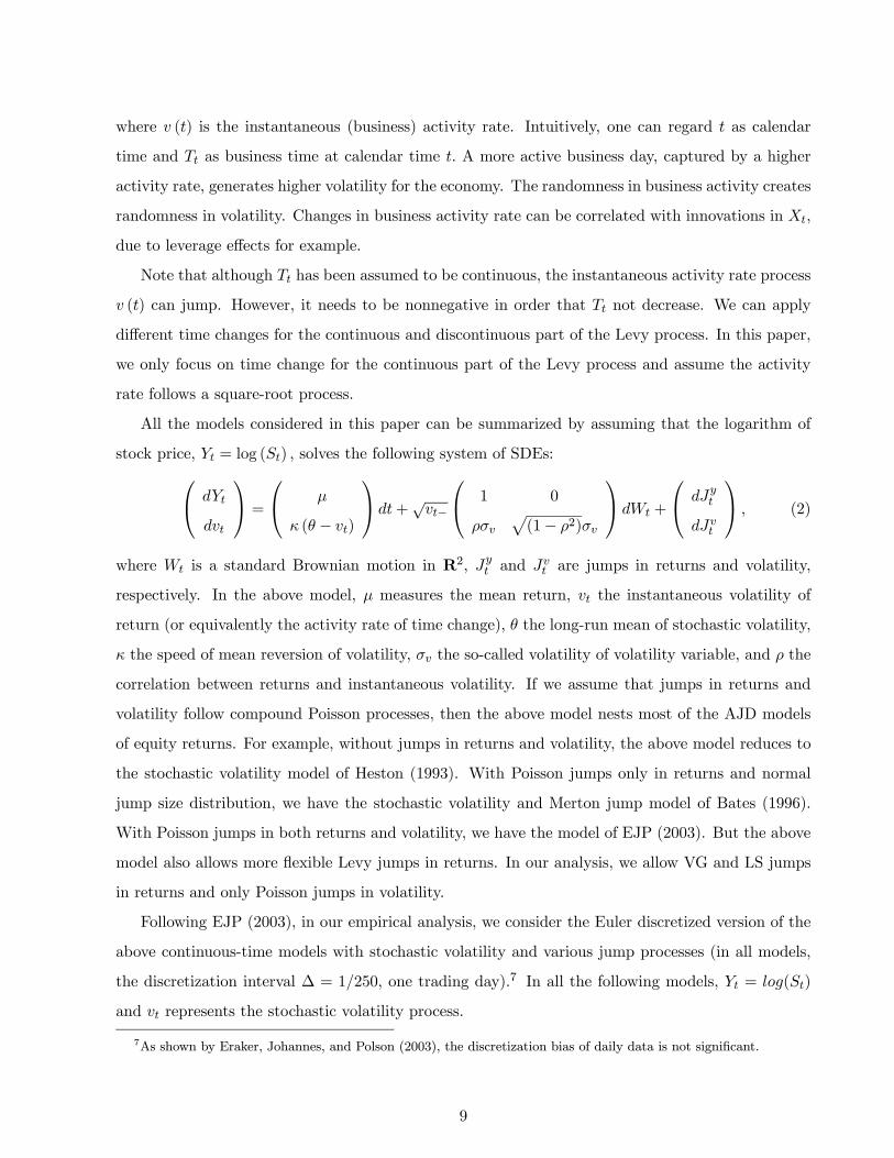
All the models considered in this paper can be summarized by assuming that the logarithm of

stock price, Yt = log (St) , solves the following system of SDEs: dYt

dvt

=

µ

κ (θ − vt)

dt+√vt−

1 0

ρσvp(1− ρ2)σv

dWt +

dJyt

dJvt

, (2)

where Wt is a standard Brownian motion in R2, Jyt and Jvt are jumps in returns and volatility,

respectively. In the above model, µ measures the mean return, vt the instantaneous volatility of

return (or equivalently the activity rate of time change), θ the long-run mean of stochastic volatility,

κ the speed of mean reversion of volatility, σv the so-called volatility of volatility variable, and ρ the

correlation between returns and instantaneous volatility. If we assume that jumps in returns and

volatility follow compound Poisson processes, then the above model nests most of the AJD models

of equity returns. For example, without jumps in returns and volatility, the above model reduces to

the stochastic volatility model of Heston (1993). With Poisson jumps only in returns and normal

jump size distribution, we have the stochastic volatility and Merton jump model of Bates (1996).

With Poisson jumps in both returns and volatility, we have the model of EJP (2003). But the above

model also allows more flexible Levy jumps in returns. In our analysis, we allow VG and LS jumps

in returns and only Poisson jumps in volatility.

Following EJP (2003), in our empirical analysis, we consider the Euler discretized version of the

above continuous-time models with stochastic volatility and various jump processes (in all models,

the discretization interval ∆ = 1/250, one trading day).7 In all the following models, Yt = log(St)

and vt represents the stochastic volatility process.

7As shown by Eraker, Johannes, and Polson (2003), the discretization bias of daily data is not significant.

9

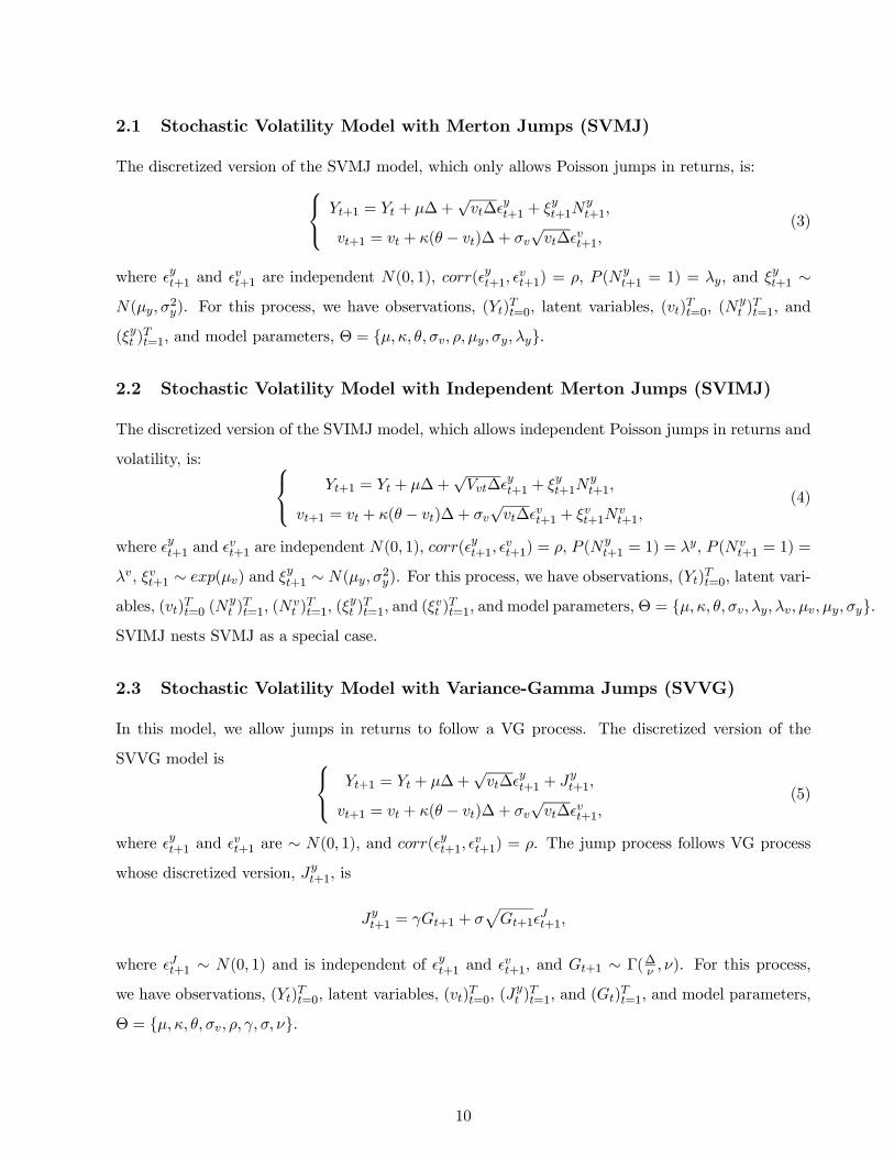
2.1 Stochastic Volatility Model with Merton Jumps (SVMJ)

The discretized version of the SVMJ model, which only allows Poisson jumps in returns, is: Yt+1 = Yt + µ∆+√vt∆

yt+1 + ξyt+1N

yt+1,

vt+1 = vt + κ(θ − vt)∆+ σv√vt∆

vt+1,

(3)

where yt+1 and

vt+1 are independent N(0, 1), corr(

yt+1,

vt+1) = ρ, P (Ny

t+1 = 1) = λy, and ξyt+1 ∼N(µy, σ

2y). For this process, we have observations, (Yt)

Tt=0, latent variables, (vt)

Tt=0, (N

yt )

Tt=1, and

(ξyt )Tt=1, and model parameters, Θ = µ, κ, θ, σv, ρ, µy, σy, λy.

2.2 Stochastic Volatility Model with Independent Merton Jumps (SVIMJ)

The discretized version of the SVIMJ model, which allows independent Poisson jumps in returns and

volatility, is: Yt+1 = Yt + µ∆+√Vvt∆

yt+1 + ξyt+1N

yt+1,

vt+1 = vt + κ(θ − vt)∆+ σv√vt∆

vt+1 + ξvt+1N

vt+1,

(4)

where yt+1 and

vt+1 are independent N(0, 1), corr(

yt+1,

vt+1) = ρ, P (Ny

t+1 = 1) = λy, P (Nvt+1 = 1) =

λv, ξvt+1 ∼ exp(µv) and ξyt+1 ∼ N(µy, σ

2y). For this process, we have observations, (Yt)

Tt=0, latent vari-

ables, (vt)Tt=0 (N

yt )

Tt=1, (N

vt )

Tt=1, (ξ

yt )

Tt=1, and (ξ

vt )

Tt=1, and model parameters, Θ = µ, κ, θ, σv, λy, λv, µv, µy, σy.

SVIMJ nests SVMJ as a special case.

2.3 Stochastic Volatility Model with Variance-Gamma Jumps (SVVG)

In this model, we allow jumps in returns to follow a VG process. The discretized version of the

SVVG model is Yt+1 = Yt + µ∆+√vt∆

yt+1 + Jyt+1,

vt+1 = vt + κ(θ − vt)∆+ σv√vt∆

vt+1,

(5)

where yt+1 and

vt+1 are ∼ N(0, 1), and corr( y

t+1,vt+1) = ρ. The jump process follows VG process

whose discretized version, Jyt+1, is

Jyt+1 = γGt+1 + σpGt+1

Jt+1,

where Jt+1 ∼ N(0, 1) and is independent of y

t+1 andvt+1, and Gt+1 ∼ Γ(∆ν , ν). For this process,

we have observations, (Yt)Tt=0, latent variables, (vt)

Tt=0, (J

yt )

Tt=1, and (Gt)

Tt=1, and model parameters,

Θ = µ, κ, θ, σv, ρ, γ, σ, ν.

10

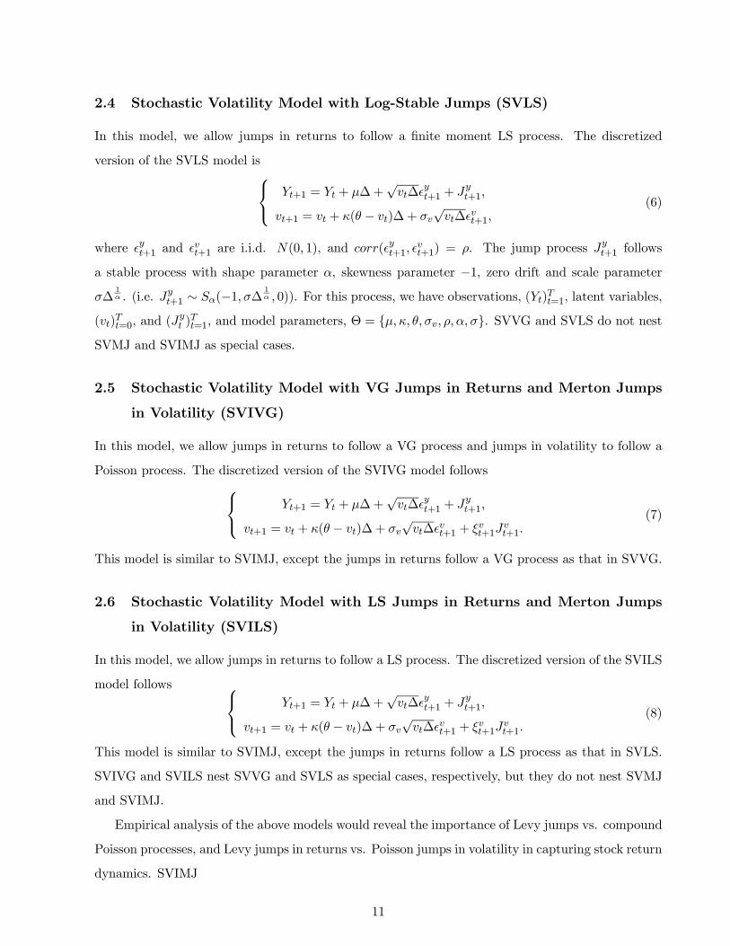
2.4 Stochastic Volatility Model with Log-Stable Jumps (SVLS)

In this model, we allow jumps in returns to follow a finite moment LS process. The discretized

version of the SVLS model is Yt+1 = Yt + µ∆+√vt∆

yt+1 + Jyt+1,

vt+1 = vt + κ(θ − vt)∆+ σv√vt∆

vt+1,

(6)

where yt+1 and

vt+1 are i.i.d. N(0, 1), and corr( y

t+1,vt+1) = ρ. The jump process Jyt+1 follows

a stable process with shape parameter α, skewness parameter −1, zero drift and scale parameterσ∆

1α . (i.e. Jyt+1 ∼ Sα(−1, σ∆ 1

α , 0)). For this process, we have observations, (Yt)Tt=1, latent variables,

(vt)Tt=0, and (J

yt )

Tt=1, and model parameters, Θ = µ, κ, θ, σv, ρ, α, σ. SVVG and SVLS do not nest

SVMJ and SVIMJ as special cases.

2.5 Stochastic Volatility Model with VG Jumps in Returns and Merton Jumps

in Volatility (SVIVG)

In this model, we allow jumps in returns to follow a VG process and jumps in volatility to follow a

Poisson process. The discretized version of the SVIVG model follows Yt+1 = Yt + µ∆+√vt∆

yt+1 + Jyt+1,

vt+1 = vt + κ(θ − vt)∆+ σv√vt∆

vt+1 + ξvt+1J

vt+1.

(7)

This model is similar to SVIMJ, except the jumps in returns follow a VG process as that in SVVG.

2.6 Stochastic Volatility Model with LS Jumps in Returns and Merton Jumps

in Volatility (SVILS)

In this model, we allow jumps in returns to follow a LS process. The discretized version of the SVILS

model follows Yt+1 = Yt + µ∆+√vt∆

yt+1 + Jyt+1,

vt+1 = vt + κ(θ − vt)∆+ σv√vt∆

vt+1 + ξvt+1J

vt+1.

(8)

This model is similar to SVIMJ, except the jumps in returns follow a LS process as that in SVLS.

SVIVG and SVILS nest SVVG and SVLS as special cases, respectively, but they do not nest SVMJ

and SVIMJ.

Empirical analysis of the above models would reveal the importance of Levy jumps vs. compound

Poisson processes, and Levy jumps in returns vs. Poisson jumps in volatility in capturing stock return

dynamics. SVIMJ

11

3 MCMC Analysis of Time-Changed Levy Processes

3.1 Overview of MCMC

One of the main challenges in empirical analysis of continuous-time models using discretely sampled

data is estimating model parameters. For most models, the transition density is generally not known

in closed-form, which renders likelihood-based approach computationally almost impossible (see, Lo

1988). In the last decade, a large number of estimation methods have been developed for estimating

continuous-time models. These include the closed-form approximated maximum likelihood approach

of Ait-Sahalia (2002, 2003); the simulated maximum likelihood approach of Pedersen (1995) and

Brandt and Santa-Clara (2002); the method of moments of Hansen and Scheinkman (1996); the

simulated method of moments of Duffie and Singleton (1993); the efficient method of moments of

Gallant and Tauchen (1996); the characteristic function approach of Chacko and Viceira (1999),

Jiang and Knight (1999), and Singleton (1999), among many others.

We face several challenges when applying the above methods to the models considered in this

paper. First, the probability density for certain Levy processes are not known in closed-form and

higher moments of asset returns do not even exist. This makes it difficult to apply existing methods

that have mainly focused on diffusion or Poisson jump-diffusion models to Levy processes. Second,

the high dimensionality of latent variables, such as stochastic volatility, jump sizes and jump times,

significantly complicates the estimation further. Computationally it is very demanding to integrate

out the vast number of latent variables when implementing either likelihood or moment-based ap-

proaches.

In this section, we adopt a Bayesian approach for the inference of time-changed Levy processes.

Specifically, we develop a computational Bayesian estimation technique for estimating the time-

changed Levy processes using Markov Chain Monte Carlo (MCMC) methods.8 As pointed out by

EJP (2003) and Johannes and Polson (2003), relative to other estimation methods, MCMC has

several advantages. For example, MCMC provides not only estimates of model parameters, but

also latent state variables, such as stochastic volatility, jump times and sizes as a by-product of the

algorithm. MCMC also automatically accounts for estimation risk. Furthermore, as shown in EJP

(2003), MCMC has excellent finite sample performance when estimating similar models. In what

8Earlier studies, such as Jacquier, Polson, and Rossi (1994), Kim, Shephard, and Chib (1998), and Chib, Nardari,

and Shephard (2003) apply MCMC methods to estimate discrete-time stochastic volatility models. Other studies that

apply MCMC methods to continuous-time models for stock price or interest rate include Jones (1998), Eraker (2001),

and Elerian, Chib, and Shephard (2001).

12

follows we provide a brief overview of the basic idea of MCMC and demonstrate how to apply the

method to compute objects of interest in Bayesian inference of stochastic processes.9

Suppose Θ is a vector of all the unknown parameters of a model, X contains all the latent

variables, such as jump times, jump sizes and volatility, andY is the observed asset price. The goal of

our statistical inference is to estimate model parameters and latent state variables from observed asset

prices. That is, we need to estimate the marginal posterior distribution p (Θ|Y) , which characterizesthe sample information about the model parameters, and p (X|Y) , which combines the model anddata to provide consistent estimates of the state variables.

MCMC for our models is a conditional simulation methodology that generates random samples

from a given target distribution. The objective of MCMC is to sample from the distribution of

parameters and latent variables given the observed prices, i.e. p(Θ,X|Y), which is typically highdimensional in our applications. MCMC samples from these high-dimensional, and complex distri-

butions by generating a Markov Chain over (Θ,X) , (Θ(g),X(g))Gg=1, whose equilibrium distribution

is p(Θ,X|Y). The Monte Carlo method uses these samples for numerical integration for parameterand state estimation, and model comparison.

MCMC algorithms are based on the commonly known Clifford-Hammersley theorem, which states

that a joint distribution can be characterized fully by its so-called complete conditional distribu-

tions. This implies that p(X|Θ,Y) and p(Θ|X,Y) completely characterize the joint distribution of

p(Θ,X|Y). The key to MCMC is that it is typically easier to simulate from the complete conditionaldistributions, p(X|Θ,Y) and p(Θ|X,Y), than to directly from the higher-dimensional joint distri-

bution, p(Θ,X|Y). MCMC provides the recipe for combining the information in these distributionsto generate samples from p(Θ,X|Y). The following is a typical MCMC algorithm. Given two initialvalues, Θ(0) and X(0), draw X(1) ∼ p(X|Θ(0),Y) and then Θ(1) ∼ p(Θ|X(1),Y). Continuing in thisfashion, the algorithm generates a sequence of random variables,

©Θ(g),X(g)

ªGg=1

. This sequence

forms a Markov Chain whose distribution, under a number of metrics and mild conditions, converges

to the target distribution p(Θ,X|Y).If the complete conditionals are known in closed form and can be directly sampled from, the

algorithm is called “Gibbs Sampler”. In many situations, one or more of the conditionals cannot be

directly sampled from, and we have to resort to the so-called “Metropolis-Hastings” method or some

of its variations. These algorithms sample a candidate draw from a proposal density and then accept

9Our discussion of MCMC in this section largely follows Johannes and Polson (2003), which provide an excellent

review of the method.

13

or reject the candidate draw based on an acceptance criterion. In practice, we often have to use the

so-called “hybrid” MCMC algorithm which combines the Gibbs and Metropolis-Hastings methods.

The samples©Θ(g),X(g)

ªGg=1

from the joint posterior can be used for parameter and state variable

estimation using the Monte Carlo method. Specifically, the estimate of (Θ,X) is the posterior mean

of p (Θ,X) , approximated by 1G

PGg=1(Θ

(g),X(g)). This is based on the fact that under certain

regularity conditions, as G→∞, the Monte Carlo average 1G

PGg=1 f(Θ

(g),X(g)) converges a.s. to

E [f (Θ,X) |Y] =Z

f (Θ,X) p(Θ,X|Y)dXdΘ.

By Bayes rule, the joint posterior density p(Θ,X|Y) can be written in the form that is pro-

portional to the product of likelihood function, distribution of latent state variables, and the prior

distribution of model parameters. That is,

p (Θ,X|Y) ∝ p (Y|X,Θ) p (X|Θ) p (Θ) ,

where Y = YtTt=1 are the observed prices, X = XtTt=1 are the unobserved state variables, Θare the parameters, p (Y|X,Θ) is the likelihood function, p (X|Θ) is the distribution of the statevariables, and p (Θ) is the prior distribution of the parameters. The parametric continuous-time

model generates p (Y|X,Θ) and p (X|Θ) , and p (Θ) summarizes any non-sample information aboutthe parameters. Since our models are Markov, the joint posterior distribution can be further written

as

p(Θ,X|Y) ∝T−1Yt=0

p(Yt+1 − Yt|Xt,Θ)×T−1Yt=0

p(Xt+1 −Xt|Θ)× p(Θ).

It is important to point out that p (Y|X,Θ) is the full-information likelihood and is different

from the marginal likelihood function, p (Y|Θ) , which integrates out the latent variables:

p (Y|Θ) =Z

p (Y,X|Θ) dX =

Zp (Y|X,Θ) p (X|Θ) dX.

In most continuous-time asset pricing models, p (Y|Θ) is not known in closed form and simulation

methods are required to perform likelihood-based inference. On the other hand, the full-information

likelihood is usually known in closed form which is a key to MCMC estimation.

Applying MCMC to p(Θ,X|Y), we can obtain estimates of model parameters and state variables.We can also use the posterior distribution to conduct both formal and informal analysis of model

performance. Informally, the posterior can be used to analyze the in-sample fit. For example, as

suggested by EJP (2003), the posterior can be used to test the normality of standardized model

residuals, taking into account estimation risk. For example, for SVMJ model, we have

Yt+1 − Yt − µ∆−Nyt+1ξ

yt+1√

vt∆= y

t+1 ∼ N (0, 1) .

14

By testing whether model residuals approximately follow a N (0, 1) distribution provides a straight-

forward way to understand potential model misspecifications.

Formal statistical inference on model performance using Bayesian diagnostic tools such as Odds

ratios or Bayes Factors can also be computed using the output of MCMC algorithms.10 With a finite

number of models under consideration, MiMi=1, we can compute the posterior odds of Mi versus

Mj ,p (Mi|Y)p (Mj |Y) =

p (Y|Mi) p (Mi)

p (Y|Mj) p (Mj),

where p (Y|Mi) is the marginal distribution ofY for modelMi.Here, the ratio, p (Y|Mi) /p (Y|Mj),

is commonly referred to as the Bayes factor, which provides a straightforward way of comparing model

performance. A good rule of thumb in the existing literature (see, Kass and Raftery 1995) is that if

-2log p(Mi|Y)p(Mj |Y) > 10, then one would preferMj toMi. One advantage of Bayes factor is that model

Mi andMj do not have to be nested as in likelihood ratio type of tests. This makes it convenient to

compare performance of continuous-time models that often do not nest each other. In the appendix,

we provide more details on how to calculate Bayes factor for model performance.

3.2 MCMC Algorithms for Time-Changed Levy Processes

In this section, we describe in more detail the MCMC algorithms for estimating time-changed Levy

processes. Our discussion here focuses on SVMJ, SVVG, and SVLS, and for each model we describe

how to simulate from the joint posterior distribution of model parameters, latent stochastic volatility

variables, jump times and jump sizes. Although the same procedure applies to most models, for

certain models, some special techniques are needed.

Conditioning on Jt+1 and vt, changes in Yt and vt follow a joint bivariate normal distribution.

That is, for m =MJ,V G, and LS, Y+1 − Yt

vt+1 − vt

|Jmt+1, vt ∼ N

µ∆− Jmt+1

κ (θ − vt)∆

, vt∆

1 ρσv

ρσv σ2v

,

where JMJt+1 = Nt+1ξt+1, J

V Gt+1 ∼ N

¡γGt+1, σ

2V GGt+1

¢, Gt+1 ∼ Γ

¡∆ν , ν

¢, and JLSt+1 ∼ Sα

³−1, σ∆ 1

α , 0´.

For the SVMJ model, it is more convenient to separate JMJt+1 into a Bernoulli variable Nt+1

indicating whether a jump occurs or not, and a continuous variable ξt+1 describes the jump size once

a jump has occurred. Thus, the joint distribution of Y, V, N, ξ and parameters Θ is

p(Y,V,N, ξ,Θ) = p(Y,V|N, ξ,Θ)p(ξ|Θ)p(N|Θ)p(Θ)10See, e.g., Kass and Raftery (1995) or Han and Carlin (2000) for reviews of the huge literature on this issue.

15

∝T−1Yt=0

1

σvvt∆p1− ρ2

exp

½− 1

2(1− ρ2)

³¡ yt+1

¢2 − 2ρ yt+1

vt+1 +

¡vt+1

¢2´¾

×T−1Yt=0

1

σyexp

½−(ξt+1 − µy)

2

2σ2y

¾×

T−1Yt=0

λNt+1y (1− λy)

1−Nt+1 × p(Θ),

where yt+1 = (Yt+1 − Yt − µ∆−Nt+1ξt+1) /

√vt∆, and

vt+1 = (vt+1 − vt − κ(θ − vt)∆) /σv

√vt∆.

For the SVVG model, the joint distribution of Y, V, JV G, G and parameters Θ is

p(Y,V,JV G,G,Θ) = p(Y,V|JV G,Θ)p(JV G|G,Θ)p(G|Θ)p(Θ)

∝T−1Yt=0

1

σvvt∆p1− ρ2

exp

½− 1

2(1− ρ2)

³¡ yt+1

¢2 − 2ρ yt+1

vt+1 +

¡vt+1

¢2´¾

×T−1Yt=0

1

σV G√Gt+1

exp

(−(J

V Gt+1 − γGt+1)

2

2σ2V GGt+1

)×

T−1Yt=0

1

ν∆ν Γ(∆ν )

G∆ν−1

t+1 exp

½−Gt+1

ν

¾,

where yt+1 =

¡Yt+1 − Yt − µ∆− JV Gt+1

¢/√vt∆, and

vt+1 is defined as before.

While it is straightforward to write down the joint distribution of observed and latent variables,

and model parameters for the SVMJ and SVVG model, the task becomes difficult for the SVLS

model. This is because the probability density of stable distribution is generally unknown, except

for some special cases.11

Fortunately, Buckle (1995) shows that by introducing an auxiliary variable U , the bivariate

probability density function of the standard stable variable S∗ = Sα(1, β, 0), and U , conditional on

α and β, is given by

p(S∗, U |α, β) = α

|α− 1|exp−|S∗

tα,β(U)|α/(α−1)| S∗

tα,β(U)|α/(α−1) 1|S∗|

×[1(S∗, U)S∗∈(−∞,0)TU∈(− 1

2,lα,β)

+ 1(S∗, U)S∗∈(0,∞)T U∈(lα,β , 12 )]

where tα,β(U) = (sin[παU+ηα,β ]

cosπU )( cosπUcos[π(α−1)U+ηα,β ])

(α−1)/α, and ηα,β = βmin(α, 2− α)π/2 and lα,β =

−ηα,β/(πα). The joint distribution of a generalized stable variable S and U can be obtained by only

transforming S∗ to S = γ + δS∗.

An extension of the data augmentation idea of Buckle (1995) allows us to use MCMC schemes

to get joint samples of JLS and U, then marginalize U out to obtain the samples for JLS. In the

11The probability density of the following three special cases of stable distribution is analytically known. For α = 2,

we have S2 (0, δ, γ) ∼ N¡γ, δ2

¢; for α = 1, we have S1 (0, δ, γ) follows a Cauchy distribution; and for α =

12 , we have

S 12(1, δ, 0) follow a Levy distribution.

16

SVLS model, we use the Log Stable Process (Carr and Wu 2003) where we set α ∈ (1, 2], β = −1,γ = 0 and δ = σ∆

1α . The joint distribution of Y, V, JLS , U and parameters Θ is

p(Y,V,JLS ,U,Θ) = p(Y,V|JLS,Θ)p(JLS,U|Θ)p(Θ)

∝T−1Yt=0

1

σvVt∆p1− ρ2

exp

½− 1

2(1− ρ2)

³¡ yt+1

¢2 − 2ρ yt+1

vt+1 +

¡vt+1

¢2´¾

×Ã

α

|α− 1|∆ 1ασ

!T

× exp−

T−1Xt=0

¯¯ JLSt+1

σ∆1∆ tα(Ut+1)

¯¯

αα−1×

T−1Yt=0

¯¯ JLSt+1

σ∆1α tα(Ut+1)

¯¯

αα−1

¯¯ σ∆

1α

JLSt+1σ∆1α

¯¯

×T−1Yt=0

[1(JLSt+1, Ut+1)Jt+1∈(−∞,0)TUt+1∈(− 1

2,lα)+ 1(JLSt+1, Ut+1)JLSt+1∈(0,∞)

TUt+1∈(lα, 12 )]× p(Θ)

where yt+1 =

¡Yt+1 − Yt − µ∆− JLSt+1

¢/√Vt∆, tα(Ut+1) = (

sin[παUt+1+(α−2)π

2]

cosπUt+1)( cosπUt+1

cos[π(α−1)Ut+1+ (α−2)π2

])(α−1)/α,

lα =2−α2α , and v

t+1 is defined as before.

For the following model parameters that are common to all three models, we choose the following

priors:

µ ∼ N(e,E2), κ ∼ N(f, F 2), θ ∼ N(g,G2), σv ∝ 1

σv, and ρ ∼ Uniform(−1, 1).

For parameters that are specific to each of the three models, we choose the following priors:

SVMJ: µy ∼ N(o,O2), σy ∝ 1

σy, and λy ∼ Uniform(0, 1);

SVVG: γ ∼ N(h,H2), σV G ∝ 1

σV G, and ν ∝ 1

ν;

SVLS: α ∼ Uniform(1, 2), and σLS ∝1

σLS.

In choosing the priors of model parameters, we try to make them as uninformative as possible.

For example, we choose flat priors for σv, ρ, σy, σV G, σLS , and λy. For other parameters, we use hyper

parameter priors on e,E, f, F, g,G, o, and O. That is, we set e, f, g, o ∼ N(0, 25), and E,F,G,O ∼G(1, 1). By adding one additional layer to hierarchy of priors, the method becomes more robust and

less dependent on which prior parameter values we use.

Given the above specification, for each model, we can obtain the joint posterior distribution of

the parameters, Θ, and the latent volatility and jump variables. The joint posterior distribution

of model parameters and latent variables is proportional to their joint distribution with Y being

17

considered as a constant. That is, we have,

for SVMJ : p (Θ,V,N, ξ|Y) ∝ p(Y,V,N, ξ,Θ);

for SVVG : p¡Θ,V,JVG,G|Y¢ ∝ p(Y,V,JV G,G,Θ);

for SVLS : p¡Θ,V,JLS,U|Y¢ ∝ p(Y,V,JLS,U,Θ).

As the above posterior distributions are quite complicated, our MCMC algorithm generates samples

by iteratively drawing from the following conditional posteriors. For example, for the g-th iteration,

we have

1. Updating model parameters:

MJ : p³Θ(g)i |Θ(g−1)−i ,N(g−1), ξ(g−1),V(g−1),Y

´, i = 1, ..., k

V G : p³Θ(g)i |Θ(g−1)−i ,JV G(g−1),G(g−1),V(g−1),Y

´, i = 1, ..., k

LS : p³Θ(g)i |Θ(g−1)−i ,JLS(g−1),U(g−1),V(g−1),Y

´, i = 1, ..., k.

2. Updating jump variables:

MJ :

p³N(g)t = 1|Θ(g), ξ(g−1)y ,V(g−1),Y

´,

p³ξy(g)t |Θ(g),J(g)t = 1, V(g−1),Y

´,

t = 1, ..., T

V G :

p³JV G(g−1)t |Θ(g),G(g−1),V(g−1),Y

´,

p³G(g)t |Θ(g),JV G(g)t , V(g−1),Y

´,

t = 1, ..., T

LS :

p³JLS(g)t |Θ(g),U(g−1),V(g−1),Y

´,

p³U(g)t |Θ(g),JLS(g)t , V(g),Y

´.

t = 1, ..., T

3. Updating volatility variables

MJ : p³V(g)t |V (g−1)t+1 , V

(g)t ,Θ(g),N(g), ξ(g),Y

´, t = 1, ..., T

V G : p³V(g)t |V (g−1)t+1 , V

(g)t ,Θ(g),JV G(g),G(g),Y

´, t = 1, ..., T

LS : p³V(g)t |V (g−1)t+1 , V

(g)t ,Θ(g),JLS(g),U(g),Y

´, t = 1, ..., T

where Θ(g−1)−i =

³θ(g)1 , ..., θ

(g)i−1, θ

(g−1)i+1 , ..., θ

(g−1)k

´.

18

4 Empirical Results

In this section, we examine the empirical performance of time-changed Levy processes in capturing

S&P 500 index returns. Compare to traditional AJDs, time-changed Levy processes have certain

advantages in modeling stock return dynamics. First, they are as flexible as AJDs in modeling the

time varying volatility of stock returns. As shown in many studies, a stochastic volatility that is

negatively correlated with returns is essential to capture S&P 500 index returns. Second, they allow

more flexible jump structures than AJDs. Jumps in compound Poisson processes are large and only

happen infrequently. For example, the parameter estimates of Andersen, Benzoni, and Lund (2002),

and EJP (2003) show that there are about three to four jumps every year in S&P 500 returns.

However, empirical observations show that stock prices exhibit frequent discontinuous movements,

both small and large. Infinite activity jump models, such as VG and LS processes are better suited

to capture such a phenomenon.

Indeed, EJP (2003) show that models with stochastic volatility and Poisson jumps in returns fail

to fully capture S&P 500 returns and jumps in volatility are also needed. They argue that while

jumps in returns only have a transient effect on asset prices, the impact of jumps in volatility is more

permanent. This is because stochastic volatility is a persistent process and a big change in volatility

dies out only slowly. Therefore, jumps in stochastic volatility help to capture movements in prices

or returns that are too large for diffusion and too small for Poisson jumps. That is, even though the

SVMJ model can capture large jumps by Poisson process and continuous movements by diffusion, it

cannot capture the many small jumps in asset prices.

While jumps in stochastic volatility is one possible way to solve this problem, time-changed Levy

processes is another potential candidate. By allowing jumps to follow Levy processes, asset prices

or returns can exhibit large rare jumps as those in Poisson models, as well as frequent small jumps.

Therefore, it is interesting to understand which alternative provides better fit of the data.

In our empirical analysis, we focus on returns of S&P 500 index from January 3, 1980 to December

31, 2000. Table I provides summary statistics of the continuously compounded returns of the index

(the log difference of index levels). The mean annual rate of return of S&P 500 is 11. 995%, and the

volatility is 16. 565%. The summary statistics of S&P 500 are very similar to that of EJP (2003)

who consider daily S&P 500 returns from January 2, 1980 to December 31, 1999.

Figure 1 plots the level and log difference of S&P 500 index. The sample period covers some

major events in the history of the US stock market, such as the stock market crash of 1987 and the

long boom in the late 1990s. The S&P 500 index declined dramatically in 1987 (-25% on October

19

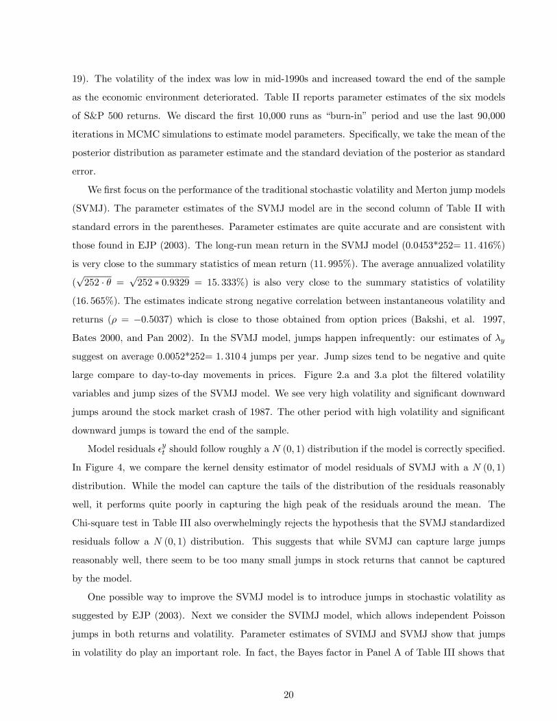
19). The volatility of the index was low in mid-1990s and increased toward the end of the sample

as the economic environment deteriorated. Table II reports parameter estimates of the six models

of S&P 500 returns. We discard the first 10,000 runs as “burn-in” period and use the last 90,000

iterations in MCMC simulations to estimate model parameters. Specifically, we take the mean of the

posterior distribution as parameter estimate and the standard deviation of the posterior as standard

error.

We first focus on the performance of the traditional stochastic volatility and Merton jump models

(SVMJ). The parameter estimates of the SVMJ model are in the second column of Table II with

standard errors in the parentheses. Parameter estimates are quite accurate and are consistent with

those found in EJP (2003). The long-run mean return in the SVMJ model (0.0453*252= 11. 416%)

is very close to the summary statistics of mean return (11. 995%). The average annualized volatility

(√252 · θ = √252 ∗ 0.9329 = 15. 333%) is also very close to the summary statistics of volatility

(16. 565%). The estimates indicate strong negative correlation between instantaneous volatility and

returns (ρ = −0.5037) which is close to those obtained from option prices (Bakshi, et al. 1997,

Bates 2000, and Pan 2002). In the SVMJ model, jumps happen infrequently: our estimates of λy

suggest on average 0.0052*252= 1. 310 4 jumps per year. Jump sizes tend to be negative and quite

large compare to day-to-day movements in prices. Figure 2.a and 3.a plot the filtered volatility

variables and jump sizes of the SVMJ model. We see very high volatility and significant downward

jumps around the stock market crash of 1987. The other period with high volatility and significant

downward jumps is toward the end of the sample.

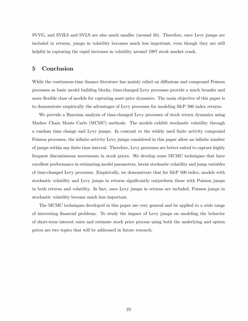
Model residuals yt should follow roughly a N (0, 1) distribution if the model is correctly specified.

In Figure 4, we compare the kernel density estimator of model residuals of SVMJ with a N (0, 1)

distribution. While the model can capture the tails of the distribution of the residuals reasonably

well, it performs quite poorly in capturing the high peak of the residuals around the mean. The

Chi-square test in Table III also overwhelmingly rejects the hypothesis that the SVMJ standardized

residuals follow a N (0, 1) distribution. This suggests that while SVMJ can capture large jumps

reasonably well, there seem to be too many small jumps in stock returns that cannot be captured

by the model.

One possible way to improve the SVMJ model is to introduce jumps in stochastic volatility as

suggested by EJP (2003). Next we consider the SVIMJ model, which allows independent Poisson

jumps in both returns and volatility. Parameter estimates of SVIMJ and SVMJ show that jumps

in volatility do play an important role. In fact, the Bayes factor in Panel A of Table III shows that

20

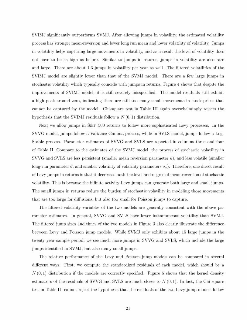
SVIMJ significantly outperforms SVMJ. After allowing jumps in volatility, the estimated volatility

process has stronger mean-reversion and lower long run mean and lower volatility of volatility. Jumps

in volatility helps capturing large movements in volatility, and as a result the level of volatility does

not have to be as high as before. Similar to jumps in returns, jumps in volatility are also rare

and large. There are about 1.3 jumps in volatility per year as well. The filtered volatilities of the

SVIMJ model are slightly lower than that of the SVMJ model. There are a few large jumps in

stochastic volatility which typically coincide with jumps in returns. Figure 4 shows that despite the

improvements of SVIMJ model, it is still severely misspecified. The model residuals still exhibit

a high peak around zero, indicating there are still too many small movements in stock prices that

cannot be captured by the model. Chi-square test in Table III again overwhelmingly rejects the

hypothesis that the SVIMJ residuals follow a N (0, 1) distribution.

Next we allow jumps in S&P 500 returns to follow more sophisticated Levy processes. In the

SVVG model, jumps follow a Variance Gamma process, while in SVLS model, jumps follow a Log-

Stable process. Parameter estimates of SVVG and SVLS are reported in columns three and four

of Table II. Compare to the estimates of the SVMJ model, the process of stochastic volatility in

SVVG and SVLS are less persistent (smaller mean reversion parameter κ), and less volatile (smaller

long-run parameter θ, and smaller volatility of volatility parameters σv). Therefore, one direct result

of Levy jumps in returns is that it decreases both the level and degree of mean-reversion of stochastic

volatility. This is because the infinite activity Levy jumps can generate both large and small jumps.

The small jumps in returns reduce the burden of stochastic volatility in modeling those movements

that are too large for diffusions, but also too small for Poisson jumps to capture.

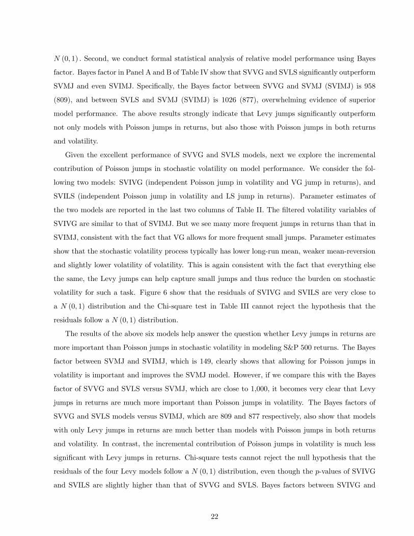
The filtered volatility variables of the two models are generally consistent with the above pa-

rameter estimates. In general, SVVG and SVLS have lower instantaneous volatility than SVMJ.

The filtered jump sizes and times of the two models in Figure 3 also clearly illustrate the difference

between Levy and Poisson jump models. While SVMJ only exhibits about 15 large jumps in the

twenty year sample period, we see much more jumps in SVVG and SVLS, which include the large

jumps identified in SVMJ, but also many small jumps.

The relative performance of the Levy and Poisson jump models can be compared in several

different ways. First, we compute the standardized residuals of each model, which should be a

N (0, 1) distribution if the models are correctly specified. Figure 5 shows that the kernel density

estimators of the residuals of SVVG and SVLS are much closer to N (0, 1). In fact, the Chi-square

test in Table III cannot reject the hypothesis that the residuals of the two Levy jump models follow

21

N (0, 1) . Second, we conduct formal statistical analysis of relative model performance using Bayes

factor. Bayes factor in Panel A and B of Table IV show that SVVG and SVLS significantly outperform

SVMJ and even SVIMJ. Specifically, the Bayes factor between SVVG and SVMJ (SVIMJ) is 958

(809), and between SVLS and SVMJ (SVIMJ) is 1026 (877), overwhelming evidence of superior

model performance. The above results strongly indicate that Levy jumps significantly outperform

not only models with Poisson jumps in returns, but also those with Poisson jumps in both returns

and volatility.

Given the excellent performance of SVVG and SVLS models, next we explore the incremental

contribution of Poisson jumps in stochastic volatility on model performance. We consider the fol-

lowing two models: SVIVG (independent Poisson jump in volatility and VG jump in returns), and

SVILS (independent Poisson jump in volatility and LS jump in returns). Parameter estimates of

the two models are reported in the last two columns of Table II. The filtered volatility variables of

SVIVG are similar to that of SVIMJ. But we see many more frequent jumps in returns than that in

SVIMJ, consistent with the fact that VG allows for more frequent small jumps. Parameter estimates

show that the stochastic volatility process typically has lower long-run mean, weaker mean-reversion

and slightly lower volatility of volatility. This is again consistent with the fact that everything else

the same, the Levy jumps can help capture small jumps and thus reduce the burden on stochastic

volatility for such a task. Figure 6 show that the residuals of SVIVG and SVILS are very close to

a N (0, 1) distribution and the Chi-square test in Table III cannot reject the hypothesis that the

residuals follow a N (0, 1) distribution.

The results of the above six models help answer the question whether Levy jumps in returns are

more important than Poisson jumps in stochastic volatility in modeling S&P 500 returns. The Bayes

factor between SVMJ and SVIMJ, which is 149, clearly shows that allowing for Poisson jumps in

volatility is important and improves the SVMJ model. However, if we compare this with the Bayes

factor of SVVG and SVLS versus SVMJ, which are close to 1,000, it becomes very clear that Levy

jumps in returns are much more important than Poisson jumps in volatility. The Bayes factors of

SVVG and SVLS models versus SVIMJ, which are 809 and 877 respectively, also show that models

with only Levy jumps in returns are much better than models with Poisson jumps in both returns

and volatility. In contrast, the incremental contribution of Poisson jumps in volatility is much less

significant with Levy jumps in returns. Chi-square tests cannot reject the null hypothesis that the

residuals of the four Levy models follow a N (0, 1) distribution, even though the p-values of SVIVG

and SVILS are slightly higher than that of SVVG and SVLS. Bayes factors between SVIVG and

22

SVVG, and SVILS and SVLS are also much smaller (around 50). Therefore, once Levy jumps are

included in returns, jumps in volatility becomes much less important, even though they are still

helpful in capturing the rapid increases in volatility around 1987 stock market crash.

5 Conclusion

While the continuous-time finance literature has mainly relied on diffusions and compound Poisson

processes as basic model building blocks, time-changed Levy processes provide a much broader and

more flexible class of models for capturing asset price dynamics. The main objective of this paper is

to demonstrate empirically the advantages of Levy processes for modeling S&P 500 index returns.

We provide a Bayesian analysis of time-changed Levy processes of stock return dynamics using

Markov Chain Monte Carlo (MCMC) methods. The models exhibit stochastic volatility through

a random time change and Levy jumps. In contrast to the widely used finite activity compound

Poisson processes, the infinite activity Levy jumps considered in this paper allow an infinite number

of jumps within any finite time interval. Therefore, Levy processes are better suited to capture highly

frequent discontinuous movements in stock prices. We develop some MCMC techniques that have

excellent performance in estimating model parameters, latent stochastic volatility and jump variables

of time-changed Levy processes. Empirically, we demonstrate that for S&P 500 index, models with

stochastic volatility and Levy jumps in returns significantly outperform those with Poisson jumps

in both returns and volatility. In fact, once Levy jumps in returns are included, Poisson jumps in

stochastic volatility become much less important.

The MCMC techniques developed in this paper are very general and be applied to a wide range

of interesting financial problems. To study the impact of Levy jumps on modeling the behavior

of short-term interest rates and estimate stock price process using both the underlying and option

prices are two topics that will be addressed in future research.

23

APPENDIX A: BAYES FACTOR

This appendix shows how to use Bayesian inference to do the model selection. Suppose we want

to compare modelM0 with modelM1. The Bayes Factor is defined as the posterior odds ofM0 being

correct versus M1

B01 =p(M0|Y)p(M1|Y) =

p(Y|M0)

p(Y|M1)

p(M0)

p(M1).

Assuming prior ignorance (i.e. p(M0)/p(M1) = 1),

B01 =p(M0|Y)p(M1|Y) =

p(Y|M0)

p(Y|M1)

Kass and Raftery (1994) suggested a rule of thumb, which is: Evidence against model M0 if

log(B10) > 10.

Calculation of B01 is easy as long as we can approximate p(Y|Mi), i = 0, 1. Since p(Y|Mi =

E[pMi(Y|Θ,X)], we can obtain the approximation of p(Y|Mi) by

p(Y|Mi) =GX

g=B

pMi(Y|Θ(g),X(g))

where g = B, ..., G are the iteration index, pMi is likelihood component under modelMi, (Θ(g),X(g))

is the posterior sample at gth iteration and B is the cutoff point for burning period. The results in

Table IV are all based on this log odds ratio.

For example, to calculate the Bayes Factor for the SVMJ model, we have

p(Y|SVMJ) =GX

g=B

T−1Yt=0

1√2π

qV(g)t ∆(1− ρ(g)2)

×

exp(−(Yt+1 − Yt − µ(g)∆J

(g)t+1ξ

(g)T+1 − ρ(g)

σ(g)v

(V(g)t+1 − V

(g)t − κ(g)(θ(g) − V

(g)t )∆))2

2V(g)t ∆(1− ρ(g)2)

)

where the items with the superscript (g) are the samples obtained from the g-th iteration.

24

REFERENCES

Ait-Sahalia, Y., 2002, Maximum-likelihood estimation of discretely sampled diffusions: A closed-form

approach, Econometrica 70, 223-262.

Ait-Sahalia, Y., 2003, Closed-form expansion for multivariate diffusions, Working paper, Princeton

University.

Anderson, T., L., Benzoni, and J. Lund, 2002, An empirical investigation of continuous-time equity

return models, Journal of Finance 57, 1239-1284.

Bakshi, G., C. Cao, and Z. Chen, 1997, Empirical performance of alternative option pricing models”,

Journal of Finance 52, 2003-2049.

Bates, D., 1996, Jumps and stochastic volatility: Exchange rate processes implicit in Deutsche mark

options, Review of Financial Studies 9, 69-107.

Bates, D., 2000, Post-’87 crash fears in S&P 500 futures options, Journal of Econometrics 94, 181-238.

Barndorff-Nielsen, O., 1998, Processes of normal inverse Gaussian type, Finance and Stochastics,

41-68.

Black, F. and M. Scholes, 1973, The Pricing of options and corporate liabilities, Journal of Political

Economy 81, 637-654.

Brandt, M., and P. Santa-Clara, 2002, Simulated likelihood estimation of diffusions with an applica-

tion to exchange rate dynamics in incomplete markets, Journal of Financial Economics 63, 161-210.

Buckle, D.J., 1995, Bayesian inference for stable distributions, Journal of the American Statistical

Association 90, 605-613.

Campbell, J., A. Lo, and C. MacKinlay, 1997, The Econometrics of Financial Markets, Princeton

University Press.

Carr, P. and L. Wu, 2003, The finite moment log stable process and option pricing, Journal of

Finance 58, 753-777.

Carr, P. and L. Wu, 2004, Time-changed Levy processes and option pricing, Journal of Financial

Economics 71, 113-141.

Carr, P., H. Geman, D. Madan, M. Yor, 2002, The fine structure of asset returns: An empirical

investigation, Journal of Business 75, 305-332.

Chacko, G., and S. Das, 2002, Pricing interest rate derivatives: A general approach, Review of

Financial Studies 15, 195-241.

Chambers, J., C. Mallows, and B. Stuck, 1976, A method for simulating stable random variables,

Journal of the American Statistical Association 71, 340-344.

25

Chernov, M., R. Gallant, E. Ghysels, and G. Tauchen, 1999, A new class of stochastic volatility

models with jumps: Theory and estimation, Working paper, Columbia University, UNC, and Duke

University.

Chernov, M., R. Gallant, E. Ghysels, and G. Tauchen, 2003, Alternative models for stock price

dynamics, Journal of Econometrics 116, 335-257.

Chernov, M., and E. Ghysels, 2000, A study towards a unified approach to the joint estimation

of objective and risk neutral measures for the purpose of options valuation, Journal of Financial

Economics 56, 407-458.

Chib, S., F. Nardari, and N. Shephard, 2002, Markov chain Monte Carlo methods for stochastic

volatility models, Journal of Econometrics 108, 281-316..

Chib, S. and E. Greenberg, 1995, Understanding the Metropolis-Hastings algorithm, Amer. Statist.

49, 327-335.

Damien, P., J. Wakefield, and S. Walker, 1999, Gibbs sampling for Bayesian non-conjugate and

hierarchical models by using auxiliary variables, Journal of Royal Statistical Society 61, 331-344.

Devroye, L., 1986, Nonuniform Random Variate Generation, New York: Springer-Verlag.

Duffie, D., J. Pan, and K. Singleton, 2000, Transform Analysis and Asset Pricing for Affine Jump-

Diffusions, Econometrica 68, 1343-1376.

Duffie, D., and K. Singleton, 1993, Simulated moments estimation of Markov models of asset prices,

Econometrica 61, 929-952.

Eberlein, E., Keller, U., and Prause, K., 1998, New insights into smile, mispricing and Value at Risk:

The hyperbolic model, Journal of Business 71, 371-405.

Elerian, O., S. Chib, and N. Shephard, 2001, Likelihood inference for discretely observed nonlinear

diffusions, Econometrica 69, 959-994.

Eraker, B., 2001, MCMC Analysis of diffusion models with applications to finance, Journal of Busi-

ness and Economic Statistics 19, 177-191.

Eraker,B., M. Johannes, and N. Polson, 2003, The impact of jumps in equity index volatility and

returns, Journal of Finance 58, 1269-1300.

Fama, E., 1965, The behavior of stock market prices, Journal of Business 38, 34-105.

Fielitz, B., and J. Rozell, 1983, Stable distributions and mixtures of distributions hypotheses for

common stock returns, Journal of the American Statistical Association 78, 28-36.

Gallant, A.R. and G. Tauchen, 1996, Which moments to match?, Econometric Theory 12, 657-681.

Gilk, W. R., 1992, Devivative-Free Adaptive Rejection Sampling for Gibbs Sampling, Bayesian Statis-

26

tics (4the ed.), Oxford University Press.

Hansen, L.P. and J.A. Scheinkman, 1995, Back to the future: Generating moment implications for

continuous time Markov processes, Econometrica 63, 767-804.

Hastings, W.K., 1970, Monte Carlo sampling methods using Markov chain and their applications,

Biometrika 57, 97-109.

Heston, S., 1993, A closed-form solution for options with stochastic volatility with applications to

bond and currency options, Review of Financial Studies 6, 327-343.

Huang, J. and L. Wu, 2003, Specification analysis of option pricing models based on time-changed

Levy processes, Journal of Finance 59, 1405-1439.

Hull, J. and A. White, 1987, The pricing of options on asset with stochastic volatilities, Journal of

Finance 42, 281-300.

Jacquier, E., N. Polson, and P. Rossi, 1994, Bayesian analysis of stochastic volatility models, Journal

of Business and Economic Statistics 12, 371-389.

Jiang, G. and J. Knight, 2002, Estimation of continuous-time processes via the empirical character-

istic function, Journal of Business and Economic Statistics 20, 198-212.

Johannes, M. and N. Polson, 2003, MCMC methods for continuous-time financial econometrics,

Handbook of Financial Econometrics forthcoming.

Jones, C., 1998, Bayesian estimation of continuous-time finance models, Working paper, Rochester

University.

Kass, R. and A. Raftery, 1994, Bayes factors, Journal of the American Statistical Association 90,

773-795.

Kim, S., N. Shephard, and S. Chib, 1998, Stochastic volatility: Likelihood inference and comparison

with ARCH models, Review of Economic Studies 65, 361-393.

Levy, P., 1924, Theorie des Erreurs. La Loide Gauss et Less Lois Exceptionells, Bull. Soc. Math 52,

49-85.

Lo, A.W., 1988, Maximum likelihood estimation of generalized Ito processes with discretely sampled

data, Econometric Theory 4, 231-247.

Madan, D., P. Carr, and E. Chang, 1998, The variance gamma process and option pricing, European

Finance Review 2, 79-105.

Mandelbrot, B., 1963, The variation of certain speculative prices, Journal of Business 36, 394-419.

Merton, R., 1973, The theory of rational option pricing, Bell Journal of Economics and Management

Science 4, 141-183.

27

Merton, R., 1976, Option pricing when the underlying stock returns are discontinuous, Journal of

Financial Economics 3, 125-144.

Murihead, R., 1982, Aspects of Multivariate Statistical Theory, New York: Wiley.

Pan, J., 2002, The jump-risk premia implicit in options: Evidence from an integrated time-series

study, Journal of Financial Economics 63, 3-50.

Pedersen, A. R., 1995, A new approach to maximum likelihood estimation for stochastic differential

equations based on discrete observations, Scandinavian Journal of Statistics 22, 55-71.

Robert, C., and G. Casella, 1999, Monte Carlo Statistical Methods, Springer.

Ripley, B.D., 1987, Stochastic Simulation, New York: John Wiley.

Rubinstein, M., 1994, Implied binomial trees, Journal of Finance 49, 771-818.

Schaumburg, E., 2000, Maximum likelihood estimation of jump processes with applications to finance,

Working paper, Northwestern University.

Singleton, K., 2001, Estimation of affine asset pricing models using the empirical characteristic

function, Journal of Econometrics 102, 111-141.

28

Table I. Summary of Continuously Compounded Returns of S&P 500 Index This table provides summary statistics of continuously compounded returns of S&P 500 index from January 3, 1980 to December 31, 2000. The continuously compounded returns are calculated as the log difference of S&P 500 index levels. Mean Volatility Skewness Kurtosis Min Max S&P 500 0.0476 1.0435 -2.3584 55.6080 -22.8997 8.7089

Table II. MCMC Estimates of Model Parameters This table provides MCMC estimates of model parameters using S&P 500 index returns from 01/03/1980 to 12/31/2000. Parameter estimates and standard errors (in parentheses) are the mean and standard deviation of posterior distributions of model parameters, respectively. In MCMC simulation, we discard the first 10,000 simulations as burn-in period use the next 90,000 simulations in estimation.

SVMJ SVVG SVLS SVIMJ SVIVG SVILS µ 0.0453

(0.0107) 0.0607

(0.0130) 0.0609

(0.0091) 0.0475

(0.0106) 0.0671

(0.0137) 0.0625

(0.0091) κ 0.0147

(0.0038) 0.0111

(0.0030) 0.0091

(0.0025) 0.0178

(0.0037) 0.0161

(0.0037) 0.0118

(0.0024) θ 0.9329

(0.1145) 0.8636

(0.1514) 0.8944

(0.1778) 0.7322

(0.0852) 0.6430

(0.0847) 0.6308 (0.092)

σv 0.1078 (0.0113)

0.1004 (0.0095)

0.0940 (0.0079)

0.0951 (0.0115)

0.0926 (0.0098)

0.0825 (0.0072)

ρ -0.5037 (0.0509)

-0.538 (0.0601)

-0.5706 (0.0444)

-0.519 (0.0545)

-0.5586 (0.0663)

-0.5981 (0.0475)

µy -2.7338 (1.3200)

-- -- -2.5093 (1.0918)

-- --

σy 4.6746 (0.9746)

-- -- 3.9114 (0.9388)

-- --

λy 0.0052 (0.0019)

-- -- 0.0056 (0.0022)

-- --

λv -- -- -- 0.0031 (0.0021)

0.0032 (0.00015)

0.0029 (0.0002)

γ -- -0.00065 (0.00026)

-- -- -0.0008 (0.0003)

--

ν -- 379.421 (0.000002)

-- -- 379.421 (0.000002)

--

σ -- 0.0605 (0.0044)

0.2536 (0.0026)

-- 0.0552 (0.0057)

0.2537 (0.0025)

µv -- -- -- 1.787 (0.0016)

1.80 (0.001)

1.7889 (0.0012)

α -- -- 1.8132 (0.00008)

-- -- 1.8132 (0.00002)

Table III. Chi-Square Test of Standard Normal of Model Residuals

This table provides Chi-Square tests of the hypothesis that the residuals of the six time-changed Levy processes should follow a N(0,1) distribution. The interval (-infinity, +infinity) is divided into (-infinity, -3), (3, infinity) and (-3,3) which is further divided into 60 segments (with width of 0.1 for each segment). After calculating the frequencies for each segment, we apply the Chi-Square test.

SVMJ SVVG SVLS SVIMJ SVIVG SVILS

Chi-Square 82.2340 69.6748 69.3326 81.5210 61.7613 56.5864 P-value 0.0245 0.1612 0.1682 0.0277 0.3777 0.5650

Table IV. Model Comparison via Bayes Factor

This table provides model performance using the Bayes Factor. Each entry represents the posterior odds ratio between the model in the corresponding column and the model in the corresponding row. We choose the prior odds ratio to be one. An entry that is bigger than one favors the model in the corresponding column. Panel A. The importance of Levy versus Poisson jumps in returns

SVIMJ SVVG SVLS SVMJ 149 958 1026

Panel B. The importance of Levy Jumps in returns versus Poisson jumps in returns and volatility

SVVG SVLS SVIMJ 809 877

Panel C. The importance of Poisson jumps in volatility in the presence of Levy jumps in returns.

SVIVG SVILS SVVG 58 SVLS 41

Figure 1. Level and log changes of the S&P 500 index from January, 1980 to December, 2000.

1980 1985 1990 1995 2000 2005450

500

550

600

650

700

7501.a. Level of S&P 500 Index from 01/03/1980 to 12/31/2000

1980 1985 1990 1995 2000 2005-30

-20

-10

0

101.b. Log Change of S&P 500 Index from 01/03/1980 to 12/31/2000

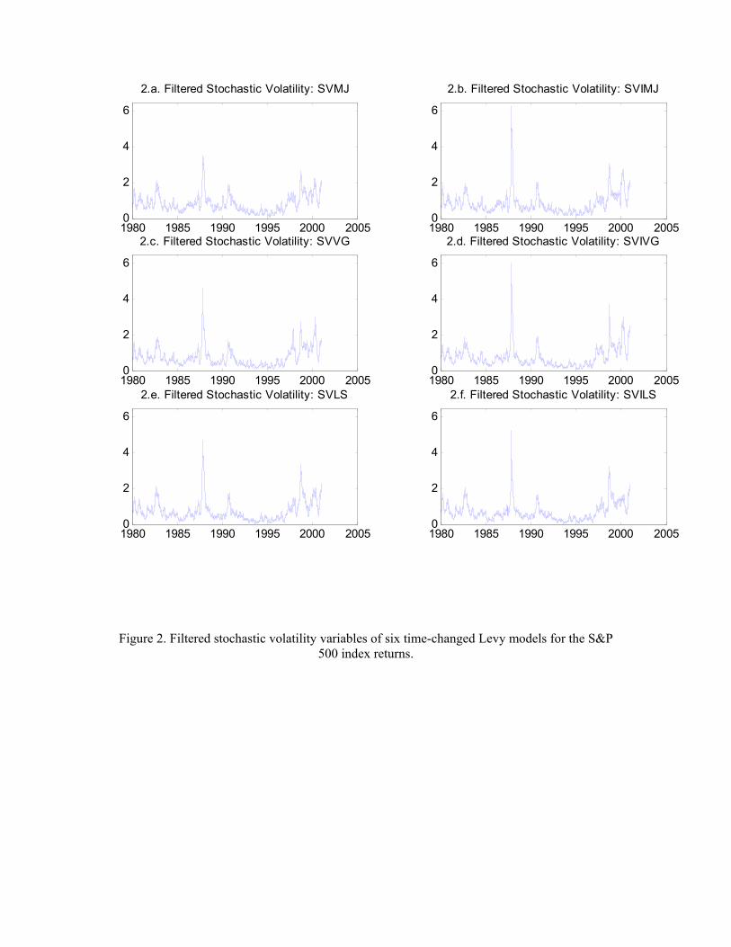
Figure 2. Filtered stochastic volatility variables of six time-changed Levy models for the S&P 500 index returns.

1980 1985 1990 1995 2000 20050

2

4

6

2.a. Filtered Stochastic Volatility: SVMJ

1980 1985 1990 1995 2000 20050

2

4

6

2.b. Filtered Stochastic Volatility: SVIMJ

1980 1985 1990 1995 2000 20050

2

4

6

2.c. Filtered Stochastic Volatility: SVVG

1980 1985 1990 1995 2000 20050

2

4

6

2.d. Filtered Stochastic Volatility: SVIVG

1980 1985 1990 1995 2000 20050

2

4

6

2.e. Filtered Stochastic Volatility: SVLS

1980 1985 1990 1995 2000 20050

2

4

6

2.f. Filtered Stochastic Volatility: SVILS

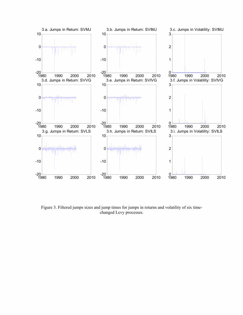
Figure 3. Filtered jumps sizes and jump times for jumps in returns and volatility of six time-changed Levy processes.

1980 1990 2000 2010-20

-10

0

103.a. Jumps in Return: SVMJ

1980 1990 2000 2010-20

-10

0

103.b. Jumps in Return: SVIMJ

1980 1990 2000 20100

1

2

33.c. Jumps in Volatility: SVIMJ

1980 1990 2000 2010-20

-10

0

103.d. Jumps in Return: SVVG

1980 1990 2000 2010-20

-10

0

103.e. Jumps in Return: SVIVG

1980 1990 2000 20100

1

2

33.f. Jumps in Volatility: SVIVG

1980 1990 2000 2010-20

-10

0

103.g. Jumps in Return: SVLS

1980 1990 2000 2010-20

-10

0

103.h. Jumps in Return: SVILS

1980 1990 2000 20100

1

2

33.i. Jumps in Volatility: SVILS

Figure 4. Comparison of kernel density estimators of the normalized residuals of the SVMJ and SVIMJ models with the density of the standard normal distribution.

-4 -2 0 2 4-4

-2

0

2

4

6

4.a. QQplot of Residuals: SVMJ

-4 -2 0 2 4-4

-2

0

2

4

6

4.b. QQplot of Residuals: SVIMJ

-4 -2 0 2 4-4

-2

0

2

4

6

4.c. QQplot of Residuals: SVVG

-4 -2 0 2 4-4

-2

0

2

4

6

4.d. QQplot of Residuals: SVIVG

-4 -2 0 2 4-4

-2

0

2

4

6

4.e. QQplot of Residuals: SVLS

-4 -2 0 2 4-4

-2

0

2

4

6

4.f. QQplot of Residuals: SVILS

-4 -3 -2 -1 0 1 2 3 40

0.05

0.1

0.15

0.2

0.25

0.3

0.35

0.4

0.45Kernel Density: SVMJKernel Density: SVIMJN(0,1)

Kernel Densities of the Residuals: SVMJ & SVIMJ

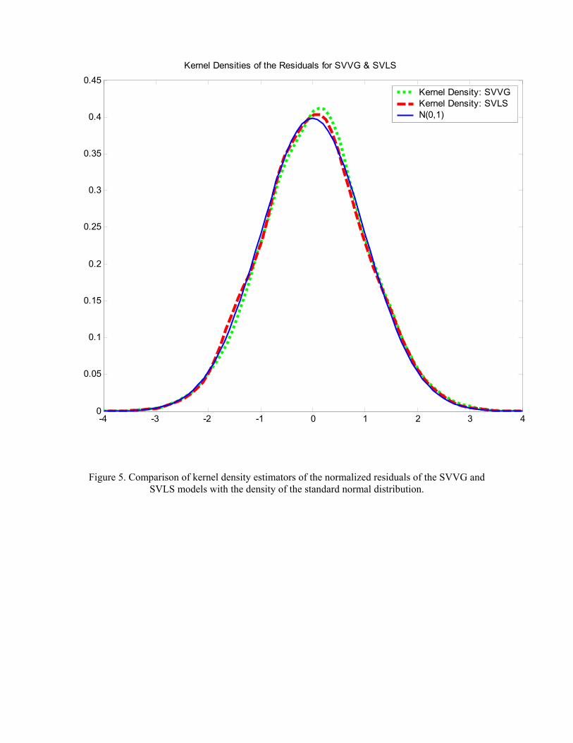
Figure 5. Comparison of kernel density estimators of the normalized residuals of the SVVG and SVLS models with the density of the standard normal distribution.

-4 -3 -2 -1 0 1 2 3 40

0.05

0.1

0.15

0.2

0.25

0.3

0.35

0.4

0.45Kernel Density: SVVGKernel Density: SVLSN(0,1)

Kernel Densities of the Residuals for SVVG & SVLS

Figure 6. Comparison of kernel density estimators of the normalized residuals of the SVIVG and SVILS models with the density of the standard normal distribution.

-4 -3 -2 -1 0 1 2 3 40

0.05

0.1

0.15

0.2

0.25

0.3

0.35

0.4

0.45Kernel Density: SVIVGKernel Density: SVILSN(0,1)

Kernel Densities of the Residuals: SVIVG & SVILS