Convergence of MCMC Algorithms in Finite Samplesecon.ucsb.edu/~doug/245a/Papers/MCMC Convergence...

Convergence of MCMC Algorithms in Finite Samples

Anna Kormilitsina and Denis Nekipelov

SMU and UC Berkeley

September 2009

Kormilitsina, Nekipelov Divergence of MCMC September 2009

Introduction

Motivation

MCMC widely used Bayesian method in frequentist context

Due to simplicity of coding and promise to converge to globalextremum, popular in structural estimation

In general requires verification of set of “regularity conditions”:practitioners rarely consider

These assumptions can be violated in very common structural models

Violation can lead to divergence of algorithm

We use example of macro DSGE model: erroneous inference can leadto misinterpretation of policy parameters


Introduction

Our approach

MCMC chain: complex dynamic system; in general, stability in suchsystems can be an issue

We use continuous-time approximation for Markov chain; allows us touse results on Lyapunov stability

Lyapunov in-stability implies divergence of MCMC chain (withprobability 1)

We formulate requirements for objective function to guaranteestability

If stability is local, convergence will not occur from some regions ofparameter space


Introduction

Our results: preview

MCMC can diverge even when structural model is identified

Create test for stability of chain initialized in particular subset ofparameter space: based on Lyapunov stability of its continuous-timeapproximation

Test creates potential for “automatic” choice of support of priordistribution

Results are illustrated using commonly used model of (Christiano,Eichenbaum, Evans, 2005)

Find that even in simple case MCMC does not have globalconvergence


Theory

Our definition of “MCMC”

MCMC - very large class of algorithms

We analyze narrow class of quasi-Bayesian procedures in(Chernozhukov, Hong, 2003)

Based on using objective for M-estimation to form a quasi-density(Laplace quasi-posterior)

Idea: convergence of statistics of quasi-posterior to extremumestimates (Bernstein-von Mises theorem) leads to convergence ofquasi-posterior moment to the M-estimator

Study this problem in the context of sampling based onMetropolis-Hastings


Theory

Characterization of Markov chains

Create sample of parameter draws from quasi-posterior

Procedure can be treated as dynamic system

Elements: proposal density, objective function + tuning parameters;output {θt}

Usually have large samples, proposals can be chosennormal/truncated normal

Sequence of draws can be approximated by diffusion-based stochasticprocess


Theory


Result from theory of SDE: form stochastic differential equation forLangevin diffusion process Lt

dLt =1

2∇ log f (Lt) dt + dWt

where Wt standard Brownian motion

f will be the stationary distribution of the solution to Langevinequation

Powerful tool: continuous mapping theorem, can look at cumulativemeans process

1√t

t∑

=0

θk

By functional continuous mapping theorem√

τt

∑

τk

θτk⇒ Lt .

This motivates us to use continuous-time approximationKormilitsina, Nekipelov Divergence of MCMC September 2009

Theory

Lyapunov stability

Dynamic system

d θt =1

2∇ log f (θt) dt + G (t, θt) dwt ,

θ0 = θ0.

Maximum of objective ⇒ equilibrium

Stochastic stability: once neighborhood of is equilibrium reached,probability of large deviations is small

Use notion of Lyapunov function

Lyapunov function V (θ, t) is non-negative continuous function, inneighborhood of equilibrium point it is bounded from above bypositive-definite function and

lim|θ|→∞

inft≥0

V (θ, t) = ∞.


Theory


Define V (·) for stochastic process θt (representation using Ito lemma)

Definition

The stochastic dynamics system is Lyapunov stable if there exists ǫ > 0and 0 < τ < ǫ such that for each t ∈ [ǫ, T − ǫ], the expectation of thesample path

E

[∫ t+τ

t−τ

dVt

∣

∣Fτ

]

≤ 0. (1)


Theory

Stability result

Theorem

Suppose θ(0) is a unique equilibrium of the MCMC stochastic process in

Θ ∈ Rk . Assume that there exists a function v : R+ × Θ → R, which is

twice continuously differentiable on its support except possibly the

equilibrium point θ(0), and v is such that

∂v(θ, t)∂t

+∑

i

12∇ log f i (θt)

∂v(t,θt )∂θt,i

+ 12

∑

i,j

{G(t,θ)G(t,θ)}i,j∂2v(t,θ)∂θi ∂θj

<0

for all (t, θ) ∈ R+ × Θ, with the strict inequality in (t, θ) ∈ R+ × Θ.

Then the equilibrium point θ(0) is asymptotically stochastically stable.


Theory

Divergence result

Theorem

Suppose θ(0) is a unique equilibrium point of MCMC stochastic process in

Θ ∈ Rk . Assume that there exists a function v : R+ × Θ → R which is

twice continuously differentiable on its support except possibly the

equilibrium point θ(0), and v is such that limθ→θ(0)

inft∈R+

v(t, θ)=∞ while

supt∈R+, θ∈Θ\Bǫ(θ(0))

{

∂v(θ, t)∂t

+∑

i

12∇ log f i (θt)

∂v(t,θt )∂θt,i

+ 12

∑

i,j

{G(t,θ)G(t,θ)}i,j∂2v(t,θ)∂θi ∂θj

}

≥0.

for Bǫ

(

θ(0)

)

={

θ∣

∣ ‖θ − θ(0)‖ < ǫ}

. Then the equilibrium point θ(0) is

asymptotically stochastically unstable and

PFt

{

supt∈R+

‖θt‖<ρ

∣

∣ θ0

}

=0,

for all θ0 ∈ Θ and 0 < ρ < diam(

Θ)

.


Theory

Implications for MCMC

Parameter chain

dθt =1

2

{

∆1T (θt) +1

π (θt)

∂π (θt)

∂θ

}

dt + dWt ,

where ∆L,T (·) is local (mean-square) gradient of quasi-likelihood

Convenient choice of Lyapunov function

v(θ) = 1{

rk−1 ≤(

θ − θ(0)

)′Σk

(

θ − θ(0)

)

≤ rk

}

ak

× exp(

αk

(

θ − θ(0)

)′Σk

(

θ − θ(0)

)

.)

Can use Σ−1 in lieu of Σk


Theory

Formal procedure

TestH0 : sup

θ∈Θ

{

{

∆1T (θt)+1

π(θt )∂π(θt )

∂θ

}

∂v(θt )

∂θ′+e′

∂2v(θt )

∂θ∂θ′e

}

<0

Formal test statistic

Ts=supt≤s

[

p∑

i,j=1

[

∆i1T

(θt)+1

π(θt )∂π(θt )

∂θit

]

Σ−1{i,j}(θjt−θ

j0)+akα2

k

∑

i,j

(

Σ−1{i,j}

)

]

.


Example

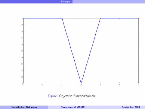
Example

Can construct simple example where MCMC has absorbing stateoutside solution

Minimize objective

Qn (θ) =1

n

n∑

i=1

(

|xi − θ|1|xi−θ|<a + a1|xi−θ|≥a

)

x ∼ U [−2a, 2a]

For well-defined a objective has well-defined minimum

Population objective is smooth

Sample objective does not sufficiently penalize outliers

Sequence of MCMC draws becomes “too stable” if the draw is farfrom true minimum


Example

−3 −2 −1 0 1 2 30

0.1

0.2

0.3

0.4

0.5

0.6

0.7

0.8

0.9

1

Figure: Objective function:sample


Example

−3 −2 −1 0 1 2 30.5

0.55

0.6

0.65

0.7

0.75

0.8

0.85

0.9

0.95

1

Figure: Objective function:population


Example

Example

Look at very simple case: accept draws if objective grows; acceptwith probability proportional to exp (Qn (θ2) − Qn (θ1)) if objectivediminishes

Statement: can choose variance of sample draws and a such that“flat region” of objective becomes absorbing state

Idea: if variance of proposal draws is large relative to a, Markov chainmoves to flat area.

There will be chains staying far from 0 for all draws


Application

Empirical application: structural model

Use DSGE model similar to (Christiano, Eichenbaum, Evans, 2005)

E0

∞∑

t=0

βtu(ct − bct−1, 1 − lt), (2)

where

u(ct , 1 − lt) = φ log(ct − bct−1) + (1 − φ) log(1 − lt), (3)

where ct − bct−1 is adjusted for habit consumption


Application

Structural model

WageW i

t = W it−1π

χw

t−1, (4)

where χw ∈ [0, 1] is the parameter of partial wage indexation

Investment

Φ

(

it

it−1

)

=κ

2

(

it

it−1− 1

)2

, (5)

Budget

Etrt,t+1xht+1 + ct + it =

xht

Πt+ trt + rtkt +

∫ 1

0w

jt

(

wjt

wt

)−η

hdt dj + φt

where trt - net transfer from government to household, φt - incomefrom ownership


Application

Structural model

Productionyi ,t ≤ ztk

1−θi ,t hi ,t

θ, (6)

Technology

log(zt

z

)

= ρz log(zt−1

z

)

+ ǫz,t , (7)

PricesP i

t = P it−1π

χp

t−1, (8)

Monetary policy

log(Rt

R) = αR log

(

Rt−1

R

)

+ απ log(πt

π

)

+ αy log

(

yt

yt−1

)

, (9)

where αR , απ, and αy - monetary policy parameters

Budget is balanced


Application

Solving structural model and generating data

Form system of Euler equations implied by equilibrium

Set parameters

Discount factorβ = .9902; Depreciation rate δ = 2.5%; Investmentadjustment costs κ = 3; habits parameter b = .6; technologyparameter θ = 0.7; price and wage rigidity αp = .6, αw = .8;indexation χp = χw = .5; elasticities of substitution ηw = ηp = 6;monetary policy rule coefficients αR = .7, απ = .45, αy = .15; inflationtarget is π = 1.005; steady state labor 0.3; steady state shadow priceof capital q = 1

Generate data for equilibrium for dynamics of macro-variables


Application

Estimator

Estimate

Θ = {αp, αw , χp, χw , b, κ, θ, β, αR , απ, αY , ρz , σz}. (10)

ObjectiveLT (θ) = (X (θ) − XT )′VT (X (θ) − XT ), (11)

X (Θ) - impulse responses generated by model, XT - impulseresponses predicted by data with T data observations

VT - weighting matrix

Use impulse responses for 20 steps of each variable: 140 points tomatch; X (θ) and XT are vectors 140 × 1, and VT is 140 × 140.


Application

Results

Smaller sample sizes lead to more frequent divergence

Compute test statistic for sample sizes: 100, 200, 500, 1000, and10, 000

Use two-step procedure: (i)run MCMC chain to find θ0 and Σ−1 (ii)Calibrate (akα2

k) = 0.026

Find that convergence quality depends on

Choice of starting valueChoice of support

Results are obtain given identification in population


Application

0.2 0.4 0.6 0.8−1000

−500

0 b

2 3 4 5−200

−100

0 κ

0.4 0.5 0.6 0.7−2000

−1000

0

αp

0.4 0.5 0.6 0.7 0.8−200

−100

0

αw

0.2 0.4 0.6 0.8−200

−100

0

χp

0.2 0.4 0.6 0.8−200

−100

0

χw

0.6 0.7 0.8 0.9−400

−200

0

αR

0.4 0.6 0.8 1−400

−200

0

απ

0.05 0.1 0.15 0.2−30

−25

−20

αy

0.1 0.15 0.2 0.25−100

−50

0

ρz

0.99 0.992 0.994 0.996 0.998−21

−20

−19 β

0.1 0.15 0.2 0.25 0.3 0.35

−400

−200

0 θ

0.6 0.8 1 1.2 1.4−4000

−2000

0

σz

Figure: Empirically evaluated expected distance function


Application

200 400 600 800 1000−14

−12

−10

−8

−6

−4

−2

x 105 10000

200 400 600 800 1000−8

−7

−6

−5

−4

−3

−2

−1

0

x 104 1000

200 400 600 800 1000

−3.5

−3

−2.5

−2

−1.5

−1

−0.5

0

0.5

x 104 500

200 400 600 800 1000

−12000

−10000

−8000

−6000

−4000

−2000

0

2000

200

200 400 600 800 1000

−7000

−6000

−5000

−4000

−3000

−2000

−1000

0

1000

2000

100

Figure: Divergence Statistics


Application

0.2 0.4 0.6 0.8

0.2

0.4

0.6

0.8

b

2 4 6

2

4

6

8

10

κ

0.2 0.4 0.6 0.8

0.5

0.6

0.7

αp

0.2 0.4 0.6 0.80.5

0.6

0.7

0.8

0.9

αw

0.2 0.4 0.6 0.8

0.2

0.4

0.6

0.8

χp

0.2 0.4 0.6 0.80.2

0.4

0.6

0.8

χw

0.6 0.7 0.8 0.9

0.6

0.7

0.8

αR

2 4 6 8

5

10

15

απ

1 2 3

1

2

3

4

αY

0.2 0.4 0.6 0.80.1

0.2

0.3

0.4

ρ

0.5 0.6 0.7 0.8 0.9

0.7

0.8

0.9

1

β

0.2 0.4 0.6 0.80.2

0.3

0.4

0.5

θ

2 4 6 8

0.8

1

1.2

1.4

σz

Figure: Dependence of estimates on starting values, 100 obs


Application

0.2 0.4 0.6 0.8

0.2

0.4

0.6

b

2 4 6

2

4

6

κ

0.2 0.4 0.6 0.8

0.2

0.4

0.6

αp

0.2 0.4 0.6 0.8

0.2

0.4

0.6

0.8

αw

0.2 0.4 0.6 0.8

0.2

0.4

0.6

0.8

χp

0.2 0.4 0.6 0.8

0.2

0.4

0.6

χw

0.6 0.7 0.8 0.9

0.6

0.7

0.8

αR

2 4 6 8

5

10

15

20

απ

1 2 3

1

2

3

4

αY

0.2 0.4 0.6 0.8

0.1

0.2

0.3

0.4

0.5 ρ

0.5 0.6 0.7 0.8 0.9

0.8

0.9

1

β

0.2 0.4 0.6 0.8

0.2

0.4

0.6

θ

2 4 6 8

0.91

1.11.21.3

σz



Application

0.2 0.4 0.6 0.8

0.2

0.4

0.6

b

2 4 6

1

2

3

κ

0.2 0.4 0.6 0.8

0.45

0.5

0.55

0.6

0.65

αp

0.2 0.4 0.6 0.8

0.5

0.6

0.7

0.8

0.9

αw

0.2 0.4 0.6 0.8

0.2

0.4

0.6

0.8

χp

0.2 0.4 0.6 0.80.1

0.2

0.3

0.4

0.5

χw

0.6 0.7 0.8 0.9

0.6

0.7

0.8

αR

2 4 6 80.4

0.6

0.8

απ

1 2 3

1

2

3

4

αY

0.2 0.4 0.6 0.80.05

0.1

0.15

0.2

ρ

0.5 0.6 0.7 0.8 0.9

0.850.9

0.951

1.05

β

0.2 0.4 0.6 0.8

0.4

0.6

0.8 θ

2 4 6 80.6

0.8

1

1.2

σz



Application

0.2 0.4 0.6 0.8

0.2

0.4

0.6

b

2 4 6

1

2

3

κ

0.2 0.4 0.6 0.80.3

0.4

0.5

0.6

αp

0.2 0.4 0.6 0.8

0.4

0.6

0.8

αw

0.2 0.4 0.6 0.8

0.2

0.4

0.6

χp

0.2 0.4 0.6 0.8

0.2

0.4

0.6

χw

0.6 0.7 0.8 0.9

0.7

0.8

0.9

αR

2 4 6 8

5

10

15

απ

1 2 3

0.5

1

1.5

2

αY

0.2 0.4 0.6 0.8

0.1

0.2

0.3

ρ

0.5 0.6 0.7 0.8 0.9

0.9

0.95

1

1.05

β

0.2 0.4 0.6 0.8

0.3

0.4

0.5

0.6 θ

2 4 6 8

0.7

0.8

0.9

1

1.1

σz



Application

0.2 0.4 0.6 0.8

0.2

0.4

0.6

b

2 4 6

1

2

3

κ

0.2 0.4 0.6 0.8

0.2

0.4

0.6

αp

0.2 0.4 0.6 0.8

0.6

0.7

0.8

αw

0.2 0.4 0.6 0.8

0.2

0.4

0.6

χp

0.2 0.4 0.6 0.80.1

0.2

0.3

0.4

0.5

χw

0.6 0.7 0.8 0.9

0.65

0.7

0.75

αR

2 4 6 8

0.4

0.45

0.5

0.55

απ

1 2 30.12

0.14

0.16

αY

0.2 0.4 0.6 0.80.2

0.4

0.6

0.8

1

ρ

0.5 0.6 0.7 0.8 0.90.9

0.95

1

1.05

β

0.2 0.4 0.6 0.8

0.4

0.6

0.8

θ

2 4 6 80.9

1

1.1

σz

Figure: Dependence of estimates on starting values, sample of 10000 observations


Convergence of MCMC Algorithms in Finite Samplesecon.ucsb.edu/~doug/245a/Papers/MCMC Convergence...

Documents

Transcript of Convergence of MCMC Algorithms in Finite Samplesecon.ucsb.edu/~doug/245a/Papers/MCMC Convergence...