European Journal of Operational Research 215 (2011) 539–550

Contents lists available at ScienceDirect

European Journal of Operational Research

journal homepage: www.elsevier .com/locate /e jor

Discrete Optimization

A mathematical programming approach to the computation of the omegainvariant of a numerical semigroup

Víctor BlancoDepartamento de Álgebra, Facultad de Ciencias, Universidad de Granada, 18071 Granada, Spain

a r t i c l e i n f o

Article history:Received 4 January 2011Accepted 4 July 2011Available online 13 July 2011

Keywords:Integer programmingMultiobjective optimizationOptimization over an efficient setNumerical semigroupsFactorization theory

0377-2217/$ - see front matter � 2011 Elsevier B.V. Adoi:10.1016/j.ejor.2011.07.004

E-mail address: vblanco@ugr.es

a b s t r a c t

In this paper we present a mathematical programming formulation for the x-invariant of a numericalsemigroup for each of its minimal generators which is an useful index in commutative algebra (in partic-ular in factorization theory) to analyze the primality of the elements in the semigroup. The model con-sists of solving a problem of optimizing a linear function over the efficient set of a multiobjectivelinear integer program. We offer a methodology to solve this problem and we provide some computa-tional experiments to show the efficiency of the proposed algorithm.

� 2011 Elsevier B.V. All rights reserved.

1. Introduction

Applying discrete optimization usually means solving real-world problems in industry, transportation, location, etc., but thereare many problems arising in abstract mathematics, specially incommutative algebra, that can be formulated as integer program-ming problems and that have centered the attention of manyresearchers. In particular, problems in classical number theoryare specially interesting and only a few papers appear in the liter-ature where operational researchers deal with these type ofproblems.

In the recent years, there have appeared several methods basedon algebraic tools to solve (single and multi-objective) discreteoptimization problems as Gröbner bases [5,8,10] or short generat-ing functions [3,6,13,14,22], amongst others. In this paper we givean inverse viewpoint, that is, how optimization tools can help tosolve algebraic problems and then getting closer both mathemati-cal fields, algebra and operational research.

Here, we study a specific problem in a basic algebraic structure:numerical semigroups. This is a simple framework where develop-ing optimization tools to make computations that are usually doneby brute force.

A numerical semigroup is a set of non-negative integers, closedunder addition, containing zero and such that its complement inZþ is finite (here Zþ stands for the set of nonnegative integer num-bers). Details about the theory of numerical semigroups can be

ll rights reserved.

found in the recent monograph by Rosales and García-Sánchez[31].

It can be checked that many of the main notions in the theory ofsemigroups are, in fact, defined or characterized as discrete optimi-zation problems. For instance, for a numerical semigroup S, itsmultiplicity, m (S), is the least nonzero integer belonging to S, thatis

mðSÞ ¼minfs 2 S n f0gg:

Note that, if the reader is not familiar with numerical semigroups,to see why the above problem is a discrete optimization problemis needed to know that any numerical semigroup is minimally gen-erated by a finite set of integers {n1, . . .,np} with gcd (n1, . . .,np) = 1,and then, any element in S can be expressed as a linear combina-tion, with non-negative integer coefficients, of this set. Hence, themultiplicity of S can be written as

mðSÞ ¼min n0 :Xp

i¼1

xini ¼ n0; x 2 Zpþ; n0 P 1; n0 2 Zþ

( ):

In this case, it is clear that m (S) = min{n1, . . . ,np}.Other well-known index is the Frobenius number. Let S be a

numerical semigroup, its Frobenius number, F (S), is the largestinteger not belonging to S. This index is well defined since by def-inition Zþ n S is finite. Then,

FðSÞ ¼maxfn 2 Z n Sg:

540 V. Blanco / European Journal of Operational Research 215 (2011) 539–550

(Note that S ¼ Zþ is a numerical semigroup with F (S) = �1 sinceZþ n S ¼ ;).

Sylvester [33] proved that when a numerical semigroup, S, isgenerated by only two elements a and b, then F (S) = ab � (a + b).However, there have not been many successes in finding formulasto compute the Frobenius number when the numerical semigroupis generated by more than two integers (see [28,29]). Unfortu-nately, it is not known, up to the moment, how to model this indexas a linear integer programming problem.

The last classical index that we want to mention is the genus ofa numerical semigroup. If S is a numerical semigroup, the genus ofS, g (S), is the cardinal of Zþ n S (its number of holes), that is,gðSÞ ¼ #Zþ n S.

New arithmetic invariants for commutative semigroups, andthen, in particular for numerical semigroups that have recently ap-peared in the literature are the tame degree, the catenary degreeand the x-invariant (see [2,7,9,17,18,20,19,26] for a complete alge-braic description of these indices). These arithmetic invariantscome from the field of commutative algebra and factorization the-ory, and their definitions are not intuitive from a combinatorialviewpoint. In particular, the x-invariant allows to derive crucialfiniteness properties in the theory of non-unique factorizationsfor semigroups (tameness). However, in [7] the authors give char-acterizations of some of these concepts that allow the optimizationapproach giving here.

The goal of this paper is to present a new method for computingthe x-invariant of a numerical semigroup by optimizing a linearfunction over set of the non-dominated solutions of a multiobjec-tive integer programming problem. In contrast to usual integerprogramming problems, in multiobjective problems there are sev-eral objective functions to be optimized. Usually, it is not possibleto optimize all the objective functions simultaneously since theobjective functions induce a partial order over the vectors in thefeasible region, so a different notion of solution is needed. A feasi-ble vector is said to be a non-dominated (or Pareto optimal)solution if no other feasible vector has component-wise largerobjective values. The evaluation through the objectives of a non-dominated solution is called efficient solution.

There are nowadays relatively few exact methods to solve gen-eral multiobjective integer and linear problems (see [16]). Some ofthem combine optimality of the returned solutions with adaptabil-ity to a wide range of problems [37,23]. Other methods, such as Dy-namic Programming, are general methods for solving, not veryefficiently, general families of optimization problems (see [35]). Adifferent approach, as the two-phase method (see [34]), looks forsupported solutions (those that can be found as solutions of a sin-gle-objective problem over the same feasible region but withobjective function a linear combination of the original objectives)in a first stage and non-supported solutions are found in a secondphase using the supported ones. The two-phase method combinesusual single-criteria methods with specific multiobjective tech-niques. In the recent paper by Özlen and Azizoglu [27] it is pro-posed a method based on solving simpler problems (having lessobjectives) multiobjective problems to enumerate the whole setof nondominated solutions although it only seems to apply, inpractice, to tri-objective problems.

Optimizing over an efficient set consists of maximizing (orminimizing) a single objective function over the solutions of amultiobjective problem. Since the structure of the solution setof that problem is in general not known, different techniques,that those used to solve single or multiobjective problems, areneeded if one wants to avoid the enumeration of all the efficientsolutions and evaluating the function over all of them. Althoughthere have appeared some papers analyzing this problem whenthe problem is continuous (see for instance, [4] or [36]), only afew study the discrete case [1,21,25]. We apply an adaptation

of the algorithm presented in [21] to compute the x-invariantof a numerical semigroup. We choose that methodology sincethe approaches given in [1,25] do not fit the requirement of ourproblem.

Although there is no need of computing the x-invariant of anumerical semigroup in a short time, the hardness of computingthis index even for a small number of generators makes it difficultto analyze the invariant. Furthermore, algebraic researchers areshowing an interest in studying certain combinatorial propertiesof non-unique factorizations (in particular by the x-invariant),but this difficulty makes it impossible to go further in the studyof this index. In [2] the authors give an algorithm to compute thex-invariant of a numerical semigroup by using techniques fromfactorization theory in monoids, and they give a short list of smallproblems that can be solved by using that methodology. We pro-vide here a new method that avoid the complete enumeration ofthe non-dominated solutions of the subjacent multiobjective prob-lem, and then, we are able to compute more efficiently the x-invariant of a numerical semigroup. This approach allows us tocompute such a invariant for semigroups for that this value cannotbe obtained by using the brute force algorithm and then, a betteranalysis of the behavior of this invariant. In the last section ofthe paper we show that our method, not only improves the CPUcomputation times, but the sizes of the problems that can besolved. However, in this paper we do not underestimate the algo-rithm in [2]. Our algorithm is able to compute the invariant for lar-ger instances, but the approach in [2] allows to give interestingconclusions for some special families of numerical semigroups thatare expressed in a parametric form. We concentrate here on thecomputational side of the problem. Other advantage of formulatingthe omega index as a mathematical programming problem is that abetter analysis of the constraints and the objective function mayimprove the efficiency of the method.

In Section 2 we introduce the preliminary definitions and re-sults for the rest of the paper. There, we describe the objects understudy, the numerical semigroups, and the index we are interestedto compute, the x-invariant. An algorithm for optimizing a linearfunction over an efficient integer set is described in Section 3. Thisapproach allows us to compute efficiently the x-invariant of anumerical semigroup. In Section 4 we show some computationaltests done to check the efficiency of the algorithm. This paper is al-most self-contained and written to be accessible for both algebra-ists and operational researchers.

2. Preliminaries

We begin this section introducing the structure under the studyof this paper. A numerical semigroup is a subset S of Zþ (here Zþdenotes the set of non-negative integers) closed under addition,containing zero and such that Zþ n S is finite. {n1, . . . ,np} is saidto be a system of generators of S if S ¼ f

Ppi¼1nixi : xi 2 Zþ; i ¼

1; . . . ; pg. We denote S = hn1, . . . ,npi if {n1, . . .,np} is a system of gen-erators of S. Note that any numerical semigroup has a unique min-imal system of generators, in the sense that no proper subset of it isa system of generators. Then, we assume through this paper thatS = hn1, . . . ,npiwhen {n1, . . . ,np} is the minimal system of generatorsof S and n1 < � � � < np. The cardinality of the minimal system of gen-erators, p, is called the embedding dimension of S and it is usuallydenoted by e(S).

Note that, for S = hn1, . . . ,npi a numerical semigroup one can de-fine a homomorphism p : Zp

þ ! S as

pðx1; . . . ; xpÞ ¼Xp

i¼1

xi ni

V. Blanco / European Journal of Operational Research 215 (2011) 539–550 541

usually called the factorization homomorphism. For any element s inS we define Z(s) as the set p�1ðsÞ ¼ x 2 Zp

þ :Pp

i¼1xini ¼ s� �

. The fac-torization monoid is the set Z (S) = p�1(S).

Example 1. Let S ¼ f0;4;6;7;8g [ fz 2 Zþ : z P 10g. It is not dif-ficult to check that S is a numerical semigroup since it is closedunder addition, contains zero and Zþ n S ¼ f1;2;3;5;9g which is afinite set. Moreover, {4,6,7} is a minimal system of generators for S,so S = h4,6,7i, being its embedding dimension e (S) = 3.

For x = (1,0,2), p(x) = (1 � 4) + (0 � 6) + (2 � 7) = 18. Actually,the factorization set for 21 is Z(21) = {(1,0,2), (0,3,0), (3,1,0)}, since(0 � 4) + (3 � 6) + (0 � 7) = (3 � 4) + (1 � 6) + (0 � 7) = 21 andthere are no more elements in Z3

þ fulfilling this condition.An element s in a numerical semigroup S (in general for any

additive semigroup) is prime if whenever x + y � s 2 S for some x,y 2 S, then either x � s 2 S or y � s 2 S. Observe that the notion ofprime element coincides with the well-known concept of primeelement in Zþ when instead of the addition operation one consid-ers the multiplicative operation in S ¼ Z. We are interested in com-puting an index that measures how far away generators of anumerical semigroup are from primes: the x-invariant (see[17,18,20,19] for further details).

Definition 2. Let S = hn1, . . . ,npi be a numerical semigroup. Fors 2 S, let x(S,s) denote the smallest N 2 Zþ [ f1g with thefollowing property:

For all n 2 Zþ and s1, . . . ,sn 2 S, ifPn

i¼1si � s 2 S, then there existsa subset X � {1, . . . ,n} such that jXj 6 N and

X

j2Xsj � s 2 S:

Furthermore, we set

xðSÞ ¼maxfxðS;niÞ : i ¼ 1; . . . ;pg 2 Zþ:

Note that x(S) <1 since any numerical semigroup satisfies theascending chain condition for v-ideals (see [7] and the referencestherein for further details). Moreover, an element s 2 S would beprime if and only if x(S,s) = 1. However, since numerical semi-groups are never factorial monoids, x(S,s) > 1 and x(S) > 1 (seefor instance [7]). For any element s 2 S, s is said to be x(S,s)-prime.

It is not direct to connect the above definition with optimizationtheory. However, the following result, proved in [7], is crucial todevelop the integer programming method proposed in this paper.Here, if A # Zp

þ, for some p P 1, we denote by Minimals A the setof minimal elements in A with respect to the component-wise or-der in Zp

þ.

Theorem 3 [7]. Let S = hn1, . . . ,npi be a numerical semigroup. Then:

1. For every n 2 S;xðS;nÞ ¼maxfPp

i¼1xi : x 2Minimals Zðnþ SÞg,and

2. xðSÞ ¼maxPp

i¼1xi : x 2MinimalsðZðni þ SÞÞ for some�

i ¼ 1; . . . ; pg.

We denote by jxj ¼Pp

i¼1xi the length of x 2 Zpþ. From the above

result, compute the x-invariant consists of maximizing the lengthsof the minimal elements in the factorization monoid.

Example 4. Let S = h4,6,7i. By using a basic brute force imple-mentation in the package numericalsgps in GAP [12], we get thatMinimals Z(4 + S) = {(0,0,2), (0,2,0), (1,0,0)}. Therefore, x(S,4) =max{2,2,1} = 2. Then, 4 is not a prime element in S but, bydefinition of x(S,4), for any set of elements in S, s1, . . . ,sn such thatPn

i¼1si � 4 2 S, there are two of those elements si and sj such thatsi + sj � 4 2 S. Thus, 4 is 2-prime element of S.

In the next section we connect the above result with the prob-lem of optimizing a linear function over the efficient set of a mul-tiobjective integer linear problem. In what follows, we recall thegeneral structure of the optimization problems that are involvedin the mathematical programming formulation of the omegainvariant. This part of the paper can be skipped if the reader isfamiliar with this theory.

An integer linear programming problem consists of finding thelargest (or smallest) value of a linear operator (objective function)c : Zn

þ ! Z when c only takes values over a feasible region definedby a system of linear equations:

a11x1 þ a12x2 þ � � � þ a1nxn ¼ b1;

. ..

am1x1 þ am2x2 þ � � � þ amnxn ¼ bm;

where aij; bj 2 Q for all i 2 {1, . . . ,m} and j 2 {1, . . . ,n}. If we denoteby A ¼ ðaijÞ 2 Qm�n and by b ¼ ðbiÞ 2 Qm, this problem can be writ-ten as

max cðxÞs:t:

Ax ¼ b;

x 2 Znþ

ðIPÞ

It is well-known [32] that the complexity of solving the above prob-lem is NP-complete, and difficult to solve even for a small numberof variables (see [11]). However, when the constraints (Ax = b) havea concrete structure, or the formulation comes from a problemwhere more information is known, it is possible to develop exact(or heuristic with high precision) algorithms that allow to solve effi-ciently this type of problems (see [24]). Recently, some papers haveappeared where algebraic tools are used to solve problem (IP) (see[10,13,22]).

If we consider in (IP) a linear operator C : Znþ ! Zk (with k P 2)

we get an integer linear multiobjective optimization problem:

max CðxÞs:t:

Ax ¼ b;

x 2 Znþ

ðMOIPÞ

Since, in this case, objective function defines a non-total order overthe set of solutions of Ax = b with x 2 Zn

þ, it is needed to define whatwe understand about solving (MOIP). We say that a vector x 2 Zn

þwith Ax = b is a non-dominated (or Pareto optimal) solution if thereis no other vector y 2 Zn

þ with Ay = b and such that C(y) 6 C(x) andC(x) – C(y) where 6 denotes the component-wise order in Zk. Then,the solution of (MOIP) is a set of feasible solutions that are not com-parable and such that we cannot find better solutions with respectto the partial ordering induced by C. In the case we want to mini-mize instead of maximize, the ordering is adapted conveniently.

In general, the complexity of solving multiobjective integer lin-ear problems is ] P-hard (see [16]) and just a few algorithms appearin the literature to solve exactly this kind of problems. The recentworks by Blanco and Puerto [5,6] and De Loera and Hemmecke [14]present algebraic approaches for solving these problems. An inter-esting monograph for multiobjective optimization is [16].

In the next and last step we recall the goal of optimizing over anefficient integer region. Note that given the set of non-dominatedsolutions of (MOIP) one may be interested in finding those non-dominated solutions that maximize a linear operator. This problemcan be formulated as:

max cðxÞs:t: x is a non-dominated solution of ðMOIPÞ:

ðOESÞ

542 V. Blanco / European Journal of Operational Research 215 (2011) 539–550

It is not possible, in general, to express the constraint of the aboveproblem as a linear system of equations. Actually, as far as we know,there are no descriptions for the set of solutions of a multiobjectiveproblem, and then, to solve (OES) one may think of solving first themultiobjective problem, and then, selecting those solutions withlargest values of c. This process is not effective and it makes it dif-ficult when the efficient set has a large size.

However, there exists a few algorithms to solve (OES) withoutenumerating the complete set of non-dominated solutions of(MOIP). In particular, we adapt the algorithm presented in [21]to solve the problem of optimizing over the efficient integer set re-lated to the x-invariant. The following result states the structure ofthe optimization problem that solves the x-invariant.

Theorem 5. Let S = hn1, . . . ,npi be a numerical semigroup. Then, foreach j 2 {1, . . . , p},x(S,nj) is the solution of the following OES problem:

max cðzÞ ¼Ppi¼1

zi

s:t: z 2min CðxÞ :¼ ðz1 ¼ x1; . . . ; zp ¼ xpÞ

s:t:Ppi¼1

xini �Ppi¼1

yini ¼ nj; ðOES0j Þ

x; y 2 Zpþ:

Proof. Observe that the elements in Minimals (Z(nj + S)) are thoseminimal elements with respect to the component wise ordering inZ(nj + S), and Zðnj þ SÞ ¼ ðx1; . . . ; xpÞ :

Ppi¼1ni xi ¼ nj þ s; for some

�s 2 Sg ¼ ðx1; . . . ; xpÞ :

Ppi¼1ni xi ¼ nj þ

Ppi¼1niyi for some yi 2

�Zþg. h

Problem ðOES0j Þ consists of maximizing the lengths of the non-

dominated solutions of a multiobjective problem. We denote by(SMOIPj) the subjacent multiobjective problem.

Denote by ej, the p-tuple having a 1 as its jth entry and zerosotherwise, for each j 2 {1, . . . ,p}. From the above result, we havethat ej 2 Z(nj + S) since we can always write nj ¼

Pi–j0 � ni þ 1 � nj

and (0, . . . ,0) is not a feasible solution. Consequently, if the multi-objective subproblem (SMOIPj) has more non-dominated solutionsthey must have xj = 0 to be not comparable with ej. The next lemmastates that these unit vector cannot be solution of the multiobjec-tive subjacent problem.

Lemma 6. Let S = hn1, . . . ,npi be a numerical semigroup. Then,x(S,nj) > 1 for all j 2 {1, . . . , p}.

Proof. From Definition 2, x(S,nj) P 1. Let us see that x(S,nj) – 1.Assume that x(S,nj) = 1, then, if

Pni¼1si � nj 2 S, there exists some

sk such that sk � nj 2 S. Equivalently, we have that nj ¼Pn

i¼1si þ sfor some s 2 S, then sk = nj + s0 for some s0 2 S, for any s1, . . . ,sn andany n 2 Zþ. It is clear that it is not possible since that assumptionimplies that the generators of S are prime, but there are no primesin a numerical semigroup (see [31]). h

Furthermore, note that the feasible region in ðOES0j Þ is not

bounded. However, by solving linear integer problems we can ob-tain upper bounds for each of the variables xi involved in the prob-lem, making bounded the feasible region. For each j 2 {1, . . . ,p} andk – j, let ubjk the optimal value of the following integer program:

ubjk :¼min xj

s:t: xjnj �Ppi¼1

yini ¼ nk;

yk ¼ 0;xj 2 Zþ; y 2 Zp

þ:

ðUBjkÞ

The solutions of (UBjk) are those feasible solutions of ðOES0j Þ in the

form xjej. An upper bound for each variable in ðOES0j Þ is then ubj =

maxk{ubjk}. In practice one may choose ubj = min{ni: i – j} to avoidthe solve the above p2 integer programming problems.

Note that if x is a non-dominated solution of the multiobjectivesubproblem in ðOES0

j Þ, and yj = 0, then xj – 0, and also, if yj – 0,then xj = 0. It is clear since if xj and yj have nonzero values, then,we can always find a feasible solution (x0,y0) where x0j ¼maxf0;xj � yjg; y0j ¼maxf0; yj � xjg, and x0i ¼ xi and y0i ¼ yi for i – j. Thisresult is also proved in [7] from an algebraic viewpoint, in termsof the supports of x and y.

As a direct consequence of Lemma 6, Theorem 5 and the com-ment above we get the following result:

Corollary 7. Let S = hn1, . . . ,npi be a numerical semigroup. Then,for each j 2 {1, . . . , p},x(S,nj) is the solution of the following OESproblem:

maxPpi¼1

zi

s:t: z 2 minðz1 ¼ x1; . . . ; zp ¼ xpÞ

s:t:Ppi¼1

xini �Ppi¼1

yini ¼ nj;

xi 6 ubi i – j;

xj ¼ 0;x; y 2 Zp

þ:

ðOESjÞ

Now, computing the x-invariant consists of solving a problemof optimizing a linear function over the efficient region of abounded integer linear multiobjective problem. In the next sectionwe describe a methodology for solving (OESj).

3. An algorithm for computing x(S,nj)

In this section we adapt the procedure given in [21] for solving(OESj), and consequently to compute the x-invariant of a numeri-cal semigroup. For the sake of that, we first give some previous re-sults related to each of the steps of the algorithm.

Let j 2 {1, . . . ,p}. The first step of the proposed procedure con-sists of stating that it is necessary to design an algorithm to com-pute x(S,nj) since this value cannot be obtained by relaxingðOES0

j Þ. With this aim, we consider a relaxed problem of (OESj) con-sisting of maximizing

Ppi¼1xi over the feasible region of the multi-

objective problem instead over the efficient solutions of it. Thisproblem reads as follows:

maxPpi¼1

xi

s:t:Ppi¼1

xini �Ppi¼1

yini ¼ nj;

xi 6 ubi i – j;

xj ¼ 0;x; y 2 Zp

þ:

ðRjÞ

If we solve (Rj) and the optimal solution is a non-dominated solu-tion of (SMOIPj), then, that solution is a solution of (OESj), sincex(S,nj) always exists. Furthermore, if (Rj) is infeasible, (OESj) hasno solution. However, in general, it is not enough to solve (Rj) toget a solution of (OESj) as illustrated with the following example.

Example 8. Let S = h4,6,7i. When solving (R1), with ub2 = ub3 = 4,we get the optimal solution x⁄ = (0,4,4). However, it is easy tocheck that there is a solution of (SMOIP1) that dominates x⁄:x ¼ ð0;2;0Þ, since 2 � 6 � 2 � 4 = 4 so it is feasible and x 6 x�.

V. Blanco / European Journal of Operational Research 215 (2011) 539–550 543

The above example justifies the development of an algorithmthat allows to improve the optimal solution of (Rj) to obtain theoptimal value of (OESj). In the next step we search for feasible solu-tions of (SMOIPj) that are non-dominated and that dominate theoptimal solution of (Rj). For that, we use the following adaptationof the result by Ecker and Kouada [15].

Lemma 9. Let x⁄ be an optimal solution of (Rj) and ð�s; �x; �yÞ an optimalsolution of the following problem

maxPpi¼1

si

s:t: xi þ si ¼ x�i i ¼ 1; . . . ;p;Ppi¼1

xini �Ppi¼1

yini ¼ n;j

xi 6 ubi i – j

xj ¼ 0;x; y 2 Zp

þ;

si P 0 i ¼ 1; . . . ; p:

ðEKjðx �gÞÞ

Then, �x is a non-dominated solution of (SMOIPj) that dominates x⁄.With this lemma, we are able to compute non-dominated solu-

tions of (SMOIPj) from the solutions of (Rj). However, these solu-tions may not be the ones that maximize the lengths in (OESj).

To move through the feasible solutions of our problem to obtainthe wished solutions, we use the idea presented in [21], where theauthor gives a procedure to generate new non-dominated solu-tions. This procedure uses the following result that also appearsin [21] and that is based on a previous result in [24].

Lemma 10 [21]. Let �x be a non-dominated solution SMOIPj and ðx; yÞan optimal solution of the following problem

maxPpi¼1

xi

s:t: xi 6 zið�xi � 1Þ �Miðzi � 1Þ i ¼ 1; . . . ;p;Ppi¼1

xini �Ppi¼1

yini ¼ nj;

xi 6 ubi i – j

xj ¼ 0;Ppi¼1

zi P 1;

x; y 2 Zpþ; z 2 f0;1gp

;

ðSjðx � ÞÞ

being Mj ¼max xj : njxj ¼Pp

i–jni yi; xi 6 ubi; i – j; x; y 2 Zpþ

n o.Then,

x is a feasible solution of (SMOIPj) that is not dominated by �x.By using the above lemma, in case the solution �x is not a solu-

tion of (OESj), we can generate other feasible solution, non compa-rable with it and such that we can check if it is the one that we aresearching or, if it is not, continue iterating to reach it.

Therefore, if the solution �x obtained is not optimal for (OESj) andwe find x by using Lemma 10, x⁄ can be replaced by x in the proce-dure of Lemma 9 to obtain a non-dominated solution that domi-nates x. If this new non-dominated solution is not the optimalsolution of (OESj) we use again Lemma 10 to obtain a non compa-rable solution with this. But it may occur that this process cyclesobtaining x again. However, this can be avoided by applying thefollowing extension of Lemma 10, that allows us to get a feasiblesolution of (SMOIPj) that is not comparable with a given list ofnon-dominated solutions �x1; . . . ; �xs.

Lemma 11 [21]. Let �x1; . . . ; �xs be non-dominated solutions of SMOIPj

and ðx; yÞ an optimal solution of the following problem

maxPpi¼1

xi

s:t: xi 6 zki

�xki � 1

� ��Mi zk

i � 1� �

i ¼ 1; . . . ;p; k ¼ 1; . . . ; sPpi¼1

xini �Ppi¼1

yini ¼ nj;

xi 6 ubi i – j;

xj ¼ 0;Ppi¼1

zki P 1 k ¼ 1; . . . ; s;

x; y 2 Zpþ; z

k 2 f0;1gp k ¼ 1; . . . ; s;

ðSjðx�1; . . . ; x�sÞÞ

and where Mj ¼max xj : njxj ¼Pp

i–jni yi; xi 6 ubi; i ¼ 1; . . . ;p; x;n

y 2 Zpþg. Actually, we can take Mj as any upper bound for xj in the mul-

tiobjective problem. In practice we choose Mj = ubj, for j = 1, . . . ,p. Then,x is a feasible solution of (SMOIPj) that is not dominated by �x1; . . . ; �xs.

With this method we are able to find a feasible solution that isnot comparable with any of the solutions found in the previousiterations (those that we know that are not optimal for (OES)).We can repeat the process until we get the desired solution, butwhen do we know that we have got the solution of our problem?To ask this question we analyze the last step of the describedprocedure.

Assume we have obtained a non-dominated solution ofð SMOIPjÞ; x. If we solve (Sj(x�1,. . .,x�s)) and we get ~x as optimal solu-tion with

Ppi¼1

~xi <Pp

i¼1xi then, x is a solution to our problem sinceamong all the possible non-dominated solutions, the one that hasmaximum length has smaller length than x. Moreover, if(Sj(x�1,. . .,x�s)) is infeasible, clearly x is our solution.

Furthermore, since the feasible region of (SMOIPj) contains a fi-nite number of points and the maximum number of steps in thealgorithm coincides with the number of nondominated solutionsof that problem, the algorithm terminates after a finite numberof iterations.

The general procedure is describe in the pseudo-code of Algo-rithm 1.

Algorithm 1: Computing the omega invariant by optimizingover an efficient set.

Input : A minimal generating system of a numericalsemigroup S: {n1, . . . ,np} and j 2 {1, . . . ,p}.

l:¼1check:¼0Solve (Rj) " x1.while check = 0 do� Set x⁄ = xl and solve (EKj(x⁄)) " xl.� Solve (Sj(x�1,. . .,x�s)) " �xl.if (Sj(x�1,. . .,x�s)) is infeasible or

Ppi¼1

�xli <

Ppi¼1xl

i then

xðS;njÞ :¼Pp

i¼1xli

check:¼1.else

Set xlþ1 :¼ x and l:¼l + 1Output :x(S,nj).

A direct consequence of all the above comments about the pro-posed procedure is the following.

Theorem 12. Let S = hn1, . . . ,npi be a numerical semigroup. Algo-rithm 1 computes x(S,nj) in a finite number of steps. The applicationof Algorithm 1 to all the minimal generators of S allows to computex(S) = max{x(S,nj): j 2 1, . . . , p}.

544 V. Blanco / European Journal of Operational Research 215 (2011) 539–550

The following example illustrates the usage of Algorithm 1.

Example 13. Let S = h4,6,7i. To compute x(S) we need to computex(S,4), x(S,6) and x(S,7). The problem (OES1) problem concerningthe computation of x(S,4) reads now:

maxP3i¼1

zi

s:t: z 2minðx1; x2; x3Þs:t: 4x1 þ 6x2 þ 7x3 � 4y1 � 6y2 � 7y3 ¼ 4;

x1 ¼ 0;x2 6 4;x3 6 4;x; y 2 Z3

þ:

ðOES01Þ

The first step of Algorithm 1 consists of solving R1:

maxP3i¼1

xi

s:t: 4x1 þ 6x2 þ 7x3 � 4y1 � 6y2 � 7y3 ¼ 4;x1 ¼ 0;x2 6 4;x3 6 4;x; y 2 Z3

þ:

ðR1Þ

An optimal solution for R1 is x1 = (0,4,4) (and y1 = (0,1,6)).Now, we start with the iterative part of Algorithm 1

First iteration.� Solve (EK (x1)), which is:

maxP3i¼1

si

s:t: x1 þ s1 ¼ 0;x2 þ s2 ¼ 4;x3 þ s3 ¼ 4;4x1 þ 6x2 þ 7x3 � 4y1 � 6y2 � 7y3 ¼ 4;x1 ¼ 0;x2 6 4;x3 6 4;x; y 2 Z3

þ

s 2 R3þ;

ðEK1ð1;4;4ÞÞ

An optimal solution for this problem is x1 ¼ ð0;2;0Þ(y ¼ ð2; 0;0Þ and s ¼ ð0;2;4Þ).

� Now, solve Sðx1Þ:

maxP3i¼1

xi

s:t: x1 6 z11ð0� 1Þ � 6ðz1

1 � 1Þ ¼ �7z11 þ 6;

x2 6 z12ð2� 1Þ � 4ðz1

2 � 1Þ ¼ �3z12 þ 4;

x3 6 z13ð0� 1Þ � 4ðz1

3 � 1Þ ¼ �5z13 þ 4;

4x1 þ 6x2 þ 7x3 � 4y1 � 6y2 � 7y3 ¼ 4;x1 ¼ 0;x2 6 4;x3 6 4;P3i¼1

zi P 1;

x; y 2 Z3þ; z1 2 f0;1g3

:

ðS1ð0;2;0ÞÞ

We get the solution �x ¼ ð0;1;4Þ (�y ¼ ð4;0;2Þ and�z1 ¼ ð0;1;0Þ).P P

Since 3

i¼1�x1i ¼ 5 P 3

i¼1x1i ¼ 2, we continue with the algo-

rithm with x2 = (0,1,4).Second iteration.� Solve EK1(x2):

maxP3i¼1

si

s:t: x1 þ s1 ¼ 0;x2 þ s2 ¼ 1;x3 þ s3 ¼ 4;4x1 þ 6x2 þ 7x3 � 4y1 � 6y2 � 7y3 ¼ 4;x1 ¼ 0;x2 6 4;x3 6 4;x; y 2 Z3

þ;

s 2 R3þ:

ðEK1ð0;1;4ÞÞ

It has as an optimal solution x2 ¼ ð0;0;2Þ ðy1 ¼ ð1;1;0Þ ands1 = (0,1,2)).

� And solve S1(x1,x2):

maxP3i¼1

xi

s:t: x1 6 z11ð0� 1Þ � 6 z1

1 � 1� �

¼ �7z11 þ 6;

x2 6 z12ð2� 1Þ � 4 z1

2 � 1� �

¼ �3z12 þ 4;

x3 6 z13ð0� 1Þ � 4 z1

3 � 1� �

¼ �5z13 þ 4;

x1 6 z21ð0� 1Þ � 6 z2

1 � 1� �

¼ �7z21 þ 6;

x2 6 z22ð0� 1Þ � 4 z2

2 � 1� �

¼ �5z22 þ 4;

x3 6 z23ð2� 1Þ � 4 z2

3 � 1� �

¼ �3z23 þ 4;

4x1 þ 6x2 þ 7x3 � 4y1 � 6y2 � 7y3 ¼ 4;x1 ¼ 0;x2 6 4;x3 6 4;P3i¼1

z1i P 1;

P3i¼1

z2i P 1;

x; y 2 Z3þ; z

1; z2 2 f0;1g3:

ðS1ð0;2;0Þ; ð0;0;2ÞÞ

which is now infeasible.P

Then xðS;4Þ ¼ 2

i¼1x2i ¼ 2. Analogously we obtain x(S,6) = 3

and x(S,7) = 5, being x(S) = max{2,3,5} = 5.

Note that further improvements can be done in the above algo-rithm by incorporating bounds for the x-invariant at each step ofit. For instance, we can initially set u0 = 0 and v0 ¼

Ppi¼1x1

i , the low-er and upper bounds for x(S,nj), respectively. Then, update u0 withthe optimal value of (EKj(x⁄)) and v0 with the optimal value of(Sj(x�1,. . .,x�s)) when they are improved. With this, we have thateither when u0 = v0 or the optimal value of (Sj(x�1,. . .,x�s)) is smallerthan u0, the solution is the last solution obtained by solving(EKj(x⁄)). We have included these bounds to our implementationfor the computational results, although some others could beadded by incorporating these bounds conveniently to the con-straints of the problems.

Moreover, if the Apery sets of the numerical semigroup areknown, the following lemma, that appears in [7], helps us to sim-plify the problem of searching minimal solutions. Recall that we

V. Blanco / European Journal of Operational Research 215 (2011) 539–550 545

denote by Ap (S,a) = {s 2 Sjs � a R S} the Apéry set of a in S (see [31]for further details).

Lemma 14 [7]. Let S = hn1, . . . ,npi be a numerical semigroup, j2 {1, . . . , p}, and (x⁄, y⁄) 2 (SMOIPj). Then, if x�i – 0;

Ppk¼1nky�k 2

ApðS;niÞ.

Proof. Choose i such that x�i – 0. Since x⁄ is feasible forðSMOIPjÞ;

Ppk¼1nk x�k ¼ nj þ

Ppk¼1nk y�k. From the minimality of

(x⁄,y⁄), x⁄ � ej cannot be minimal, that is,Pp

k¼1nkx�k � ni cannot beexpressed as an integer linear combination of n1, . . . ,np, or equiva-lently,

Ppk¼1nkx�k � nj � ni ¼ nj þ

Ppk¼1nky�k � nj R S. This implies thatPp

k¼1nky�k 2 ApðS;niÞ. h

Then, with the above result, the equation defining the feasibleregion of (SMOIPj) can be written asXp

k¼1

nkxk ¼ nj þw w 2[i–j

ApðS;niÞ ð3:1Þ

Since the above constraint is not linear, we can add part of the infor-mation contained on it by incorporating inequalities in the formPp

i¼1ni yi 6maxSp

i¼1ApðS;niÞ orPpi¼1ni yi P min

Spi¼1ApðS;niÞ ¼ minfn1; . . . ; npg:

Remark 15. Note that the complexity of solving general multiob-jective integer linear programming problems is #P-hard (see [16]).Furthermore, when fixing the dimension of the space, in our case2p, where p is the embedding dimension of the numericalsemigroup, the multiobjective problem is solvable by using apolynomial-space polynomial-space procedure with short gener-ating functions (see [6]). Then, for any j = 1, . . . ,p, computing anoptimal solution of (OESj) can be done in polynomial time for fixedp. The current implementation in GAP (brute force) has exponen-tial time complexity even fixing the embedding dimension.

4. Computational experiments

In this section we present the results of some computationalexperiments performed to analyze the applicability of the algo-rithm proposed in Section 3. For the sake of that we have generateda set of instances of numerical semigroups with different numbersof minimal generators. From the computational viewpoint, up to

Table 1Battery of numerical semigroups for the computational experiments.

name minimal generating system

S5(1) {20,354,402,417,429}S5(2) {7,292,359,645,755}S5(3) {5,86,99,148,152}S5(4) {41,65,155,317,377}S5(5) {28,55,125,233,590}

S10(1) {43,63,68,108,120,135,142,150,177,224}S10(2) {15,46,58,89,108,114,117,126,130,173}S10(3) {20,22,24,26,54,77,83,89,93,95}S10(4) {96,131,136,171,173,239,278,287,364,483}S10(5) {146,173,207,359,426,548,604,606,657,702}

S15(1) {36,47,65,79,82,84,91,96,100,109,121,124,134S15(2) {46,115,155,286,289,341,342,348,393,436,445S15(3) {40,84,126,130,132,135,142,152,165,183,217,2S15(4) {75,104,114,128,216,219,241,271,309,310, 321S15(5) {29,50,95,96,99,109,110,119,131,134,135, 152

S20(1) {131,145,249,257,260,319,354,459,465,469,48S20(2) {57,105,182,186,201,204,254,259,263,274,275S20(3) {85,298,333,342,349,358,401,415,462,480,556S20(4) {81,107,168,194,230,236,274,277,286,290,305S20(5) {101,141,279,314,329,369,399,425,438,447,47

the moment, we can only compare our algorithm with a recentimplementation done in GAP [12] (available upon request), andthat consists of enumerating all the feasible solutions of (SMOIPj),comparing them to determine which are the minimal solutions,and finally selecting those with largest length.

Our algorithm has been implemented in XPRESS-Mosel 7.0 thatallows to solve the single-objective integer problems involved inthe resolution of the x-invariant, by using a branch-and-boundmethod and nesting models by calling the library mmjobs. Thealgorithms have been executed on a PC with an Intel Core 2 Quadprocessor at 2x 2.50 Ghz and 4 GB of RAM.

The computational complexity of the algorithm depends of thedimension of the space (embedding dimension of the numericalsemigroups) and the size of the coefficients in the constraints(the minimal generators of the semigroup). Then, we have gener-ated for each p 2 {5,10,15, 20}, five instances of p non-negativeintegers ranging in [2,1000]. Note that larger instances are difficultto find since even for p = 20, selecting 20 non-negative integerswith great common divisor equal to one and such that they are aminimal system of generators of a numerical semigroup is not aneasy task. We have used recursively the function RandomListF-

orNS of GAP to get the lists of integer with the above require-ments. In Table 1 we show the battery of numerical semigroupfor which we have run the algorithms. In the first column we writethe name we give to the semigroup, in the second column the set ofminimal generating system of the numerical semigroup, and in thelast column the embedding dimension of the semigroup. Observealso that for a numerical semigroup with embedding dimensionp, the dimensions of the problems to be solved with our methodol-ogy are: 2 � p for (Rj), 3 � p for (EKj(x⁄)), and p � (2 + s) for (Sj(x�1,. . .,x�s)) (where s is the number of previously computed nondomi-nated solutions).

We summarize the obtained results in Tables 2 and 3. In thefirst column we write the numerical semigroup (S). The second col-umn is the generator with respect to the x-invariant is computed(nj). The value of x(S,nj) is shown in the third column (in this samecolumn we mark in bold face, for each numerical semigroup, themaximum value that coincides with x(S)). One of the minimal vec-tors that reach the maximum length is shown in the fourth col-umn. The next column, the fifth, shows the number of iterationsof our algorithm (it) which coincides with the number of timesthat the problems (EKj) and (Sj) are solved in Algorithm 1 TheCPU time (in seconds) needed to compute x(S, nj) with our

embdim

5

10

,139,169} 15,449,504,527,584}21,229,273,323},327,340,352,371},162,180,201}

7,572,575,587,606,607,652,674,694,762} 20,294,295,298,307,338,367,393,417,431},569,583,609,619,708,710,752,821,853},310,348,351,366,379,396,416,521,583}7,501,534,536,555,574,620,727,786,871}

Table 2Results of computational experiments for p = 5,10.

S nj x(S,nj) min it timej GAPtime tottime avtime #min

S5(1) 20 4 [0,0,0,0, 4] 9 0.54 6.03 12354 60 [60,0,0,0,0] 12 0.95 11.35 14402 63 [63,0,0,0,0] 16 1.439 12.54 5.921 1.184 17417 60 [60,0,0,0,0] 15 1.43 12.68 16429 60 [60,0,0,0,0] 17 1.55 12.43 20

S5(2) 7 3 [0,3,0,0,0] 10 0.55 12.48 11292 93 [93,0,0,0,0] 9 0.37 23.72 11359 93 [93,0,0,0,0] 11 0.43 27.33 2.84 0.56 13645 200 [200,0,0,0,0] 14 0.67 45.92 15755 200 [200,0,0,0,0] 18 0.81 75.59 19

S5(3) 5 2 [0,0,0,2,0] 8 0.285 1.201 1186 37 [37,0,0,0,0] 11 0.294 2.527 1299 37 [37,0,0,0,0] 11 0.34 2.82 1.69 0.33 12

148 60 [60,0,0,0,0] 12 0.37 4.1 13152 60 [60,0,0,0,0] 12 0.39 2.29 13

S5(4) 41 14 [0,14,0,0,0] 12 0.893 5.64 1465 22 [22,0,0,0,0] 13 0.988 6.02 14

155 24 [24,0,0,0,0] 16 1.1 8.22 7.39 1.47 18317 22 [21,0,1,0,0] 22 2.916 13.96 28377 31 [31,0,0,0,0] 18 1.49 18.7 35

S5(5) 28 10 [0,10,0,0,0] 11 0.5 10.71 1255 25 [25,0,0,0,0] 8 0.381 11.45 12

125 27 [27,0,0,0,0] 13 0.71 20.18 4.719 0.94 15233 26 [26,0,0,0,0] 13 0.732 42.37 17590 30 [24,5,0,1,0] 23 2.38 109.38 48

S10(1) 43 5 [0,0,5,0,0,0,0,0,0,0] 49 3.36 5.41 5863 8 [8,0,0,0,0,0,0,0,0,0] 48 2.7 8.61 6568 8 [8,0,0,0,0,0,0,0,0,0] 49 3.16 13.18 69

108 7 [5,0,2,0,0,0,0,0,0,0] 52 4.15 18.26 81120 8 [8,0,0,0,0,0,0,0,0,0] 57 4.24 12.65 94135 9 [9,0,0,0,0,0,0,0,0,0] 68 5.95 15.5 67.89 6.78 108142 9 [9,0,0,0,0,0,0,0,0,0] 88 9.24 16.75 125150 7 [4,2,1,0,0,0,0,0, 0,0] 66 8.07 19.85 116177 9 [7,2,0,0,0,0,0,0,0,0] 70 6.88 49.26 149224 9 [7,0,2,0,0,0,0,0,0,0] 113 20.1 65.16 246

S10(2) 15 3 [0,0,3,0,0,0,0,0,0,0] 36 1.801 6.64 4546 9 [9,0,0,0,0,0,0,0,0,0] 39 1.66 10.32 4858 10 [10,0,0,0,0,0,0,0,0,0] 38 1.69 12.23 5089 9 [7,0,1,0,0,0,0,1,0,0] 47 2.681 17.33 68

108 15 [15,0,0,0,0,0,0,0,0, 0] 63 3.278 24 83114 16 [16,0,0,0,0,0,0,0,0, 0] 57 3.07 28.81 35.87 3.58 78117 15 [15,0,0,0,0,0,0,0,0, 0] 63 4.316 21.65 88126 16 [16,0,0,0,0,0,0,0,0, 0] 73 4.243 22.48 99130 22 [22,0,0,0,0,0,0,0,0, 0] 64 3.399 38.59 98173 23 [23,0,0,0,0,0,0,0,0, 0] 107 9.73 80.49 161

S10(3) 20 4 [0,0,0,4,0,0,0,0,0,0] 39 1.48 5.1 4322 5 [5,0,0,0,0,0,0,0,0,0] 43 1.59 5.41 4524 5 [5,0,0,0,0,0,0,0,0,0] 36 1.3 5.41 4526 5 [3,2,0,0,0,0,0,0,0,0] 33 1.64 3.49 4454 6 [0,6,0,0,0,0,0,0,0,0] 52 2.77 14.05 99.49 9.94 8877 9 [7,0,2,0,0,0,0,0,0,0] 93 13.27 26.72 17683 9 [6,0,2,1,0,0,0,0, 0,0] 109 19.41 33.83 19889 10 [10,0,0,0,0,0,0,0,0,0] 100 13.85 41.18 21993 10 [10,0,0,0,0,0,0,0,0,0] 109 21.75 46.17 25495 10 [10,0,0,0,0,0,0,0,0,0] 114 22.4 52.46 251

S10(4) 131 7 [5,0,0,0,2,0,0,0,0,0] 63 8.34 61.44 102136 6 [3,1,0,0,2,0,0,0, 0,0] 47 7.23 54.38 88171 6 [2,2,0,0,2,0,0,0, 0,0] 65 11.18 56.92 102173 7 [3,1,3,0,0,0,0,0, 0,0] 60 9.87 116.22 118239 8 [5,2,0,0,0,0,0,1,0,0] 83 16.81 104.66 225.55 22.55 155278 10 [10,0,0,0,0,0,0,0,0,0] 80 14.93 129.1 208287 10 [10,0,0,0,0,0,0,0,0,0] 62 11.628 128.1 178364 10 [7,3,0,0,0,0,0,0,0,0] 128 34.053 227.12 260483 11 [9,1,0,0,0,0,1,0, 0,0] 204 105.146 497 427

S10(5) 146 8 [0,6,2,0,0,0,0,0,0,0] 42 8.048 100.82 70173 10 [10,0,0,0,0,0,0,0,0,0] 71 15.43 115.39 99207 10 [10,0,0,0,0,0,0,0,0,0] 60 11.77 138.87 82359 12 [7,5,0,0,0,0,0,0,0,0] 60 14.69 198.246 152426 12 [12,0,0,0,0,0,0,0,0, 0] 77 16.23 290.08 315.14 31.51 130548 12 [0,12,0,0,0,0,0,0,0, 0] 105 38.525 470.76 209

546 V. Blanco / European Journal of Operational Research 215 (2011) 539–550

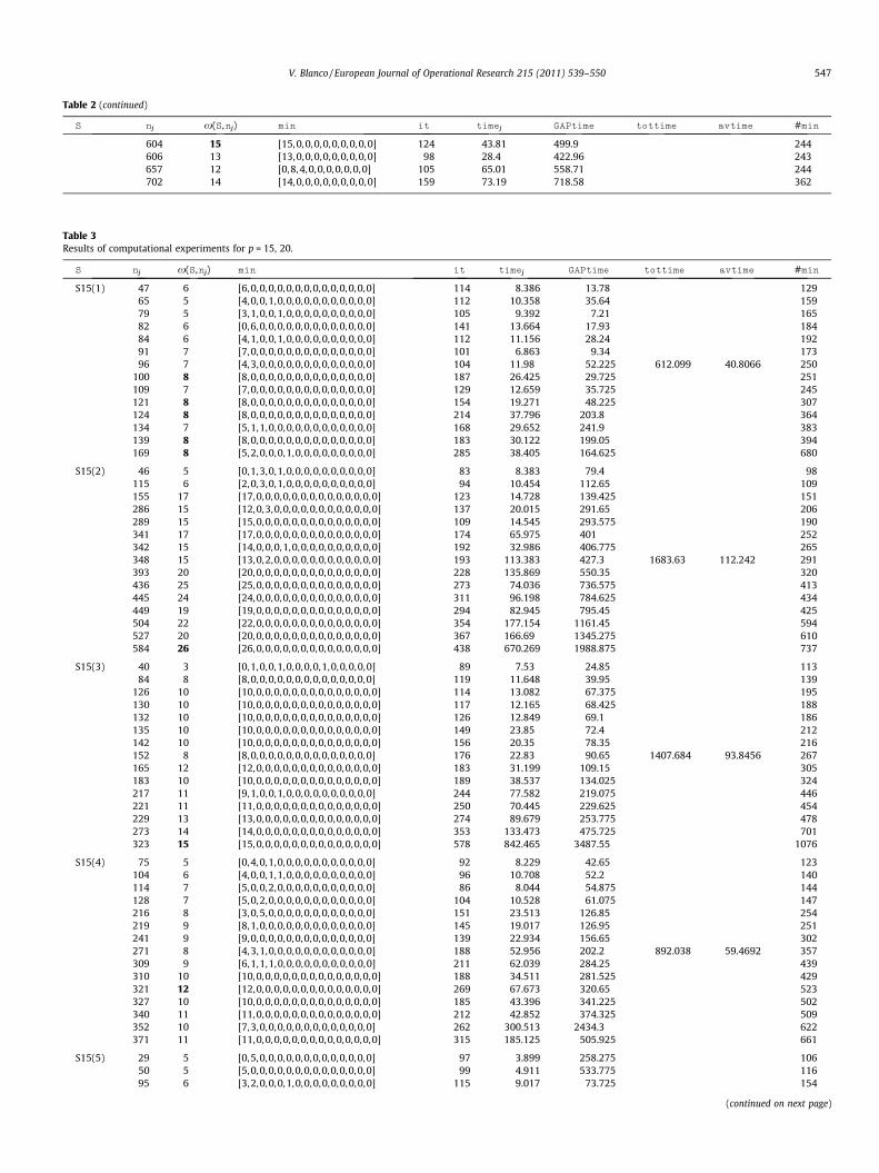
Table 2 (continued)

S nj x(S,nj) min it timej GAPtime tottime avtime #min

604 15 [15,0,0,0,0,0,0,0, 0,0] 124 43.81 499.9 244606 13 [13,0,0,0,0,0,0,0, 0,0] 98 28.4 422.96 243657 12 [0,8,4,0,0,0,0,0,0, 0] 105 65.01 558.71 244702 14 [14,0,0,0,0,0,0,0, 0,0] 159 73.19 718.58 362

Table 3Results of computational experiments for p = 15, 20.

S nj x(S,nj) min it timej GAPtime tottime avtime #min

S15(1) 47 6 [6,0,0,0,0,0,0,0,0,0,0,0, 0,0,0] 114 8.386 13.78 12965 5 [4,0,0,1,0,0,0,0,0,0, 0,0,0,0,0] 112 10.358 35.64 15979 5 [3,1,0,0,1,0,0,0, 0,0,0,0,0,0,0] 105 9.392 7.21 16582 6 [0,6,0,0,0,0,0,0,0,0,0,0, 0,0,0] 141 13.664 17.93 18484 6 [4,1,0,0,1,0,0,0, 0,0,0,0,0,0,0] 112 11.156 28.24 19291 7 [7,0,0,0,0,0,0,0,0,0,0,0, 0,0,0] 101 6.863 9.34 17396 7 [4,3,0,0,0,0,0,0,0,0, 0,0,0,0,0] 104 11.98 52.225 612.099 40.8066 250

100 8 [8,0,0,0,0,0,0,0,0,0,0,0, 0,0,0] 187 26.425 29.725 251109 7 [7,0,0,0,0,0,0,0,0,0,0,0, 0,0,0] 129 12.659 35.725 245121 8 [8,0,0,0,0,0,0,0,0,0,0,0, 0,0,0] 154 19.271 48.225 307124 8 [8,0,0,0,0,0,0,0,0,0,0,0, 0,0,0] 214 37.796 203.8 364134 7 [5,1,1,0,0,0,0,0, 0,0,0,0,0,0,0] 168 29.652 241.9 383139 8 [8,0,0,0,0,0,0,0,0,0,0,0, 0,0,0] 183 30.122 199.05 394169 8 [5,2,0,0,0,1,0,0, 0,0,0,0,0,0,0] 285 38.405 164.625 680

S15(2) 46 5 [0,1,3,0,1,0,0,0, 0,0,0,0,0,0,0] 83 8.383 79.4 98115 6 [2,0,3,0,1,0,0,0, 0,0,0,0,0,0,0] 94 10.454 112.65 109155 17 [17,0,0,0,0,0,0,0,0, 0,0,0,0,0,0] 123 14.728 139.425 151286 15 [12,0,3,0,0,0, 0,0,0,0,0,0,0,0,0] 137 20.015 291.65 206289 15 [15,0,0,0,0,0,0,0,0, 0,0,0,0,0,0] 109 14.545 293.575 190341 17 [17,0,0,0,0,0,0,0,0, 0,0,0,0,0,0] 174 65.975 401 252342 15 [14,0,0,0,1,0, 0,0,0,0,0,0,0,0,0] 192 32.986 406.775 265348 15 [13,0,2,0,0,0, 0,0,0,0,0,0,0,0,0] 193 113.383 427.3 1683.63 112.242 291393 20 [20,0,0,0,0,0,0,0,0,0,0, 0,0,0,0] 228 135.869 550.35 320436 25 [25,0,0,0,0,0,0,0,0, 0,0,0,0,0,0] 273 74.036 736.575 413445 24 [24,0,0,0,0,0,0,0,0, 0,0,0,0,0,0] 311 96.198 784.625 434449 19 [19,0,0,0,0,0,0,0,0, 0,0,0,0,0,0] 294 82.945 795.45 425504 22 [22,0,0,0,0,0,0,0,0, 0,0,0,0,0,0] 354 177.154 1161.45 594527 20 [20,0,0,0,0,0,0,0,0,0,0, 0,0,0,0] 367 166.69 1345.275 610584 26 [26,0,0,0,0,0,0,0,0, 0,0,0,0,0,0] 438 670.269 1988.875 737

S15(3) 40 3 [0,1,0,0,1,0,0,0,0,1,0,0,0,0,0] 89 7.53 24.85 11384 8 [8,0,0,0,0,0,0,0,0,0,0,0, 0,0,0] 119 11.648 39.95 139

126 10 [10,0,0,0,0,0,0,0,0,0,0, 0,0,0,0] 114 13.082 67.375 195130 10 [10,0,0,0,0,0,0,0,0,0,0, 0,0,0,0] 117 12.165 68.425 188132 10 [10,0,0,0,0,0,0,0,0,0,0, 0,0,0,0] 126 12.849 69.1 186135 10 [10,0,0,0,0,0,0,0,0,0,0, 0,0,0,0] 149 23.85 72.4 212142 10 [10,0,0,0,0,0,0,0,0,0,0, 0,0,0,0] 156 20.35 78.35 216152 8 [8,0,0,0,0,0,0,0,0,0,0,0, 0,0,0] 176 22.83 90.65 1407.684 93.8456 267165 12 [12,0,0,0,0,0,0,0,0, 0,0,0,0,0,0] 183 31.199 109.15 305183 10 [10,0,0,0,0,0,0,0,0,0,0, 0,0,0,0] 189 38.537 134.025 324217 11 [9,1,0,0,1,0,0,0, 0,0,0,0,0,0,0] 244 77.582 219.075 446221 11 [11,0,0,0,0,0,0,0,0, 0,0,0,0,0,0] 250 70.445 229.625 454229 13 [13,0,0,0,0,0,0,0,0, 0,0,0,0,0,0] 274 89.679 253.775 478273 14 [14,0,0,0,0,0,0,0,0, 0,0,0,0,0,0] 353 133.473 475.725 701323 15 [15,0,0,0,0,0,0,0,0, 0,0,0,0,0,0] 578 842.465 3487.55 1076

S15(4) 75 5 [0,4,0,1,0,0,0,0,0,0, 0,0,0,0,0] 92 8.229 42.65 123104 6 [4,0,0,1,1,0,0,0, 0,0,0,0,0,0,0] 96 10.708 52.2 140114 7 [5,0,0,2,0,0,0,0,0,0, 0,0,0,0,0] 86 8.044 54.875 144128 7 [5,0,2,0,0,0,0,0,0,0, 0,0,0,0,0] 104 10.528 61.075 147216 8 [3,0,5,0,0,0,0,0,0,0, 0,0,0,0,0] 151 23.513 126.85 254219 9 [8,1,0,0,0,0,0,0,0,0, 0,0,0,0,0] 145 19.017 126.95 251241 9 [9,0,0,0,0,0,0,0,0,0,0,0, 0,0,0] 139 22.934 156.65 302271 8 [4,3,1,0,0,0,0,0, 0,0,0,0,0,0,0] 188 52.956 202.2 892.038 59.4692 357309 9 [6,1,1,1,0,0, 0,0,0,0,0,0,0,0,0] 211 62.039 284.25 439310 10 [10,0,0,0,0,0,0,0,0,0,0, 0,0,0,0] 188 34.511 281.525 429321 12 [12,0,0,0,0,0,0,0,0, 0,0,0,0,0,0] 269 67.673 320.65 523327 10 [10,0,0,0,0,0,0,0,0,0,0, 0,0,0,0] 185 43.396 341.225 502340 11 [11,0,0,0,0,0,0,0,0, 0,0,0,0,0,0] 212 42.852 374.325 509352 10 [7,3,0,0,0,0,0,0,0,0, 0,0,0,0,0] 262 300.513 2434.3 622371 11 [11,0,0,0,0,0,0,0,0, 0,0,0,0,0,0] 315 185.125 505.925 661

S15(5) 29 5 [0,5,0,0,0,0,0,0,0,0,0,0, 0,0,0] 97 3.899 258.275 10650 5 [5,0,0,0,0,0,0,0,0,0,0,0, 0,0,0] 99 4.911 533.775 11695 6 [3,2,0,0,0,1,0,0, 0,0,0,0,0,0,0] 115 9.017 73.725 154

(continued on next page)

V. Blanco / European Journal of Operational Research 215 (2011) 539–550 547

Table 3 (continued)

S nj x(S,nj) min it timej GAPtime tottime avtime #min

96 10 [10,0,0,0,0,0,0,0,0,0,0,0, 0,0,0] 120 7.652 24.55 17199 9 [9,0, 0,0,0,0,0,0,0,0,0,0,0,0, 0] 127 9.08 25.7 170

109 9 [9,0, 0,0,0,0,0,0,0,0,0,0,0,0, 0] 138 11.984 30.225 187110 10 [10,0,0,0,0,0,0,0,0,0,0,0, 0,0,0] 124 7.249 31.025 192119 11 [11,0,0,0,0,0,0,0,0,0, 0,0,0,0,0] 127 9.411 36.375 685.921 45.72807 211131 10 [9,1,0,0,0,0,0,0,0,0,0, 0,0,0,0] 121 10.939 45.3 252134 11 [11,0,0,0,0,0,0,0,0,0, 0,0,0,0,0] 174 17.188 48.075 258135 11 [11,0,0,0,0,0,0,0,0,0, 0,0,0,0,0] 173 20.678 225.525 288152 10 [8,2,0,0,0,0,0,0,0,0,0, 0,0,0,0] 180 28.469 144.375 338162 9 [8,0, 0,0,1,0,0,0,0,0,0, 0,0,0,0] 205 32.88 83.55 357180 10 [8,2,0,0,0,0,0,0,0,0,0, 0,0,0,0] 269 71.89 269.85 471201 14 [14,0,0,0,0,0,0,0,0,0, 0,0,0,0,0] 306 440.674 1883.525 584

S20(1) 131 8 [0,8,0,0,0,0,0,0,0,0,0,0,0,0, 0,0,0,0,0,0] 188 35.321 321.325 264145 8 [8,0, 0,0,0,0,0,0,0,0,0,0,0,0, 0,0,0,0,0,0] 191 34.252 332.3 265249 9 [6,2,0,1,0,0,0,0,0, 0,0,0,0,0,0,0,0,0,0,0] 233 54.57 550.725 340257 9 [6,2,0,1,0,0,0,0,0, 0,0,0,0,0,0,0,0,0,0,0] 233 53.913 569.15 352260 8 [8,0, 0,0,0,0,0,0,0,0,0,0,0,0, 0,0,0,0,0,0] 197 47.428 573.775 355319 9 [1,7,0,1,0,0,0,0,0, 0,0,0,0,0,0,0,0,0,0,0] 244 90.809 785.925 451354 9 [4,5,0,0,0,0,0,0,0,0,0, 0,0,0,0,0,0,0,0,0] 256 97.12 938.925 500459 10 [0,10,0,0,0,0,0,0,0,0,0,0, 0,0,0,0,0,0,0,0] 398 182.085 1700.525 787465 9 [9,0, 0,0,0,0,0,0,0,0,0,0,0,0, 0,0,0,0,0,0] 356 363.725 1747.575 752469 11 [3,8,0,0,0,0,0,0,0,0,0, 0,0,0,0,0,0,0,0,0] 317 239.548 1802.75 19603.67 980.1835 796487 9 [9,0, 0,0,0,0,0,0,0,0,0,0,0,0, 0,0,0,0,0,0] 384 408.842 2011.8 865572 12 [6,6,0,0,0,0,0,0,0,0,0, 0,0,0,0,0,0,0,0,0] 399 826.33 3290.4 1160575 10 [0,10,0,0,0,0,0,0,0,0,0,0, 0,0,0,0,0,0,0,0] 542 3123.4 3414.425 1235587 12 [12,0,0,0,0,0,0,0,0,0, 0,0,0,0,0,0,0,0,0,0] 487 1356.94 3657.525 1273606 11 [11,0,0,0,0,0,0,0,0,0, 0,0,0,0,0,0,0,0,0,0] 507 2100.84 4119.5 1389607 10 [5,5,1,0,1,0,1,0,0,0,0,0,0,0,0,0, 0,0,0,0] 787 2894.21 4181.7 1387652 11 [9,0, 0,0,0,3,0,0,0,0,0, 0,0,0,0,0,0,0,0,0] 683 2013.25 5538.2 1673674 12 [12,0,0,0,0,0,0,0,0,0, 0,0,0,0,0,0,0,0,0,0] 821 1999.747 6288.875 1732694 11 [11,0,0,0,0,0,0,0,0,0, 0,0,0,0,0,0,0,0,0,0] 726 2991.08 7185.075 1851762 12 [12,0,0,0,0,0,0,0,0,0, 0,0,0,0,0,0,0,0,0,0] 118 690.26 11142.2 2375

S20(2) 57 4 [0,2,0,0,1,0,0,0,0,0,0, 0,0,1,0,0,0,0,0,0] 146 15.003 108.725 186105 7 [7,0, 0,0,0,0,0,0,0,0,0,0,0,0, 0,0,0,0,0,0] 169 20.95 158.525 211182 9 [6,3,0,0,0,0,0,0,0,0,0, 0,0,0,0,0,0,0,0,0] 195 31.558 311.125 304186 11 [11,0,0,0,0,0,0,0,0,0, 0,0,0,0,0,0,0,0,0,0] 272 61.55 328.45 364201 14 [14,0,0,0,0,0,0,0,0,0, 0,0,0,0,0,0,0,0,0,0] 319 300.1 374.2 409204 9 [9,0, 0,0,0,0,0,0,0,0,0,0,0,0, 0,0,0,0,0,0] 284 63.721 394.55 427254 9 [8,0, 0,0,1,0,0,0,0,0,0, 0,0,0,0] 378 153.266 635.725 599259 10 [7,3,0,0,0,0,0,0,0,0,0, 0,0,0,0,0,0,0,0,0] 295 72.789 653.9 530263 10 [6,4,0,0,0,0,0,0,0,0,0, 0,0,0,0,0,0,0,0,0] 294 69.81 695.8 612274 9 [4,5,0,0,0,0,0,0,0,0,0, 0,0,0,0,0,0,0,0,0] 336 172.839 751.05 11703.9 585.1952 587275 11 [8,3,0,0,0,0,0,0,0,0,0, 0,0,0,0,0,0,0,0,0] 414 217.261 798.075 702294 8 [5,1,1,0,1,0,0, 0,0,0,0,0,0,0,0,0,0,0, 0,0] 359 396.194 915.575 612295 11 [8,3,0,0,0,0,0,0,0,0,0, 0,0,0,0,0,0,0,0,0] 488 2342.7 975.65 802298 12 [12,0,0,0,0,0,0,0,0,0, 0,0,0,0,0,0,0,0,0,0] 463 174.03 990.675 773307 10 [6,4,0,0,0,0,0,0,0,0,0, 0,0,0,0,0,0,0,0,0] 391 187.431 1084.4 808338 13 [13,0,0,0,0,0,0,0,0,0, 0,0,0,0,0,0,0,0,0,0] 484 432.837 1546.65 1001367 14 [14,0,0,0,0,0,0,0,0,0, 0,0,0,0,0,0,0,0,0,0] 608 2000.37 2113.475 1248393 12 [3,9,0,0,0,0,0,0,0,0,0, 0,0,0,0,0,0,0,0,0] 658 2531.045 2889.325 1502417 11 [5,0, 2,0,0,0,0,0,0,2,3,0,0,0,0,0,0,0, 0,0] 563 1093.34 3737.325 1686431 14 [6,8,0,0,0,0,0,0,0,0,0, 0,0,0,0,0,0,0,0,0] 781 1367.11 ⁄ ⁄

S20(3) 85 4 [0,4,0,0,0,0,0,0,0,0,0,0,0,0, 0,0,0,0,0,0] 147 25.646 341.175 230298 15 [15,0,0,0,0,0,0,0,0,0, 0,0,0,0,0,0,0,0,0,0] 316 99.513 864.5 455333 15 [15,0,0,0,0,0,0,0,0,0, 0,0,0,0,0,0,0,0,0,0] 322 91.273 1007.75 465342 16 [16,0,0,0,0,0,0,0,0,0, 0,0,0,0,0,0,0,0,0,0] 326 99.809 1026.075 466349 16 [16,0,0,0,0,0,0,0,0,0, 0,0,0,0,0,0,0,0,0,0] 307 76.393 1075.375 512358 15 [15,0,0,0,0,0,0,0,0,0, 0,0,0,0,0,0,0,0,0,0] 324 86.003 1092.975 480401 12 [10,0,0,0,0,2,0,0,0,0, 0,0,0,0,0,0,0,0,0,0] 394 154.683 1372.975 631415 16 [16,0,0,0,0,0,0,0,0,0, 0,0,0,0,0,0,0,0,0,0] 448 293.327 1474 687462 15 [15,0,0,0,0,0,0,0,0,0, 0,0,0,0,0,0,0,0,0,0] 361 135.922 1827.75 691480 14 [14,0,0,0,0,0,0,0,0,0, 0,0,0,0,0,0,0,0,0,0] 527 261.581 1982.85 8912.075 445.6038 786556 16 [16,0,0,0,0,0,0,0,0,0, 0,0,0,0,0,0,0,0,0,0] 610 592.666 2975.05 1028569 18 [18,0,0,0,0,0,0,0,0,0, 0,0,0,0,0,0,0,0,0,0] 695 2453.98 3284.75 1158583 19 [19,0,0,0,0,0,0,0,0,0, 0,0,0,0,0,0,0,0,0,0] 711 1496.19 3440.55 1164609 15 [15,0,0,0,0,0,0,0,0,0, 0,0,0,0,0,0,0,0,0,0] 57 11.671 4037.25 1290619 13 [12,0,0,0,0,0,0,0,0,0, 0,0,0,0,0,0,0,0,0,0] 912 990.061 4518.725 1386708 18 [18,0,0,0,0,0,0,0,0,0, 0,0,0,0,0,0,0,0,0,0] 582 569.397 ⁄ ⁄710 15 [11,3,0,0,0,0,0,0, 0,0,0,0,0,0,0,0,0,0,0, 0] 733 673.064 ⁄ ⁄752 18 [18,0,0,0,0,0,0,0,0,0, 0,0,0,0,0,0,0,0,0,0] 777 722.174 ⁄ ⁄821 21 [18,0,0,0,0,0,1,0, 0,0,0,0,0,0,0,0,0,0,0, 0] 108 35.333 ⁄ ⁄853 21 [19,0,0,0,0,1,0,0, 0,0,0,0,0,0,0,0,0,0,0, 0] 108 43.389 ⁄ ⁄

548 V. Blanco / European Journal of Operational Research 215 (2011) 539–550

Table 3 (continued)

S nj x(S,nj) min it timej GAPtime tottime avtime #min

S20(4) 81 5 [0,5,0,0,0,0,0,0,0,0,0,0, 0,0,0,0,0,0,0,0] 140 17.706 219.175 214107 6 [6,0,0,0,0,0,0,0,0,0,0,0, 0,0,0,0,0,0,0,0] 176 27.955 264.375 251168 9 [7,2,0,0,0,0,0,0,0,0, 0,0,0,0,0,0,0,0,0,0] 185 26.037 416.725 291194 9 [6,3,0,0,0,0,0,0,0,0, 0,0,0,0,0,0,0,0,0,0] 239 57.189 527.75 427230 8 [4,4,0,0,0,0,0,0,0,0, 0,0,0,0,0,0,0,0,0,0] 186 39 707.575 471236 9 [7,2,0,0,0,0,0,0,0,0, 0,0,0,0,0,0,0,0,0,0] 198 49.312 735.875 474274 9 [8,0,1,0,0,0,0,0,0,0, 0,0,0,0,0,0,0,0,0,0] 284 524.051 1027.225 590277 9 [7,2,0,0,0,0,0,0,0,0, 0,0,0,0,0,0,0,0,0,0] 276 113.266 1079.7 679286 9 [6,2,1,0,0,0,0,0, 0,0,0,0,0,0,0,0,0,0,0, 0] 321 676.315 1143.675 698290 8 [1,7,0,0,0,0,0,0,0,0, 0,0,0,0,0,0,0,0,0,0] 312 1775.88 1177.15 11215.3 560.7652 630305 10 [7,3,0,0,0,0,0,0,0,0, 0,0,0,0,0,0,0,0,0,0] 256 188.763 1345.125 683310 10 [10,0,0,0,0,0,0,0,0,0,0, 0,0,0,0,0,0,0,0,0] 297 85.818 1407.6 704348 10 [7,3,0,0,0,0,0,0,0,0, 0,0,0,0,0,0,0,0,0,0] 403 392.226 2039.675 953351 11 [11,0,0,0,0,0,0,0,0, 0,0,0,0,0,0,0,0,0,0,0] 432 193.712 2079.4 949366 10 [9,0,0,1,0,0,0,0,0,0, 0,0,0,0,0,0,0,0,0,0] 383 295.208 2346.175 912379 10 [3,7,0,0,0,0,0,0,0,0, 0,0,0,0,0,0,0,0,0,0] 296 1007.8 2735.2 1116396 11 [10,1,0,0,0,0,0,0,0, 0,0,0,0,0,0,0,0,0,0,0] 560 3095.66 3283.85 1222416 12 [12,0,0,0,0,0,0,0,0, 0,0,0,0,0,0,0,0,0,0,0] 541 693.549 ⁄ ⁄521 14 [14,0,0,0,0,0,0,0,0, 0,0,0,0,0,0,0,0,0,0,0] 611 955.771 ⁄ ⁄583 14 [14,0,0,0,0,0,0,0,0, 0,0,0,0,0,0,0,0,0,0,0] 982 1000.085 ⁄ ⁄

S20(5) 101 8 [0,8,0,0,0,0,0,0,0,0,0,0, 0,0,0,0,0,0,0,0] 57 8.393 488.75 246141 7 [7,0,0,0,0,0,0,0,0,0,0,0, 0,0,0,0,0,0,0,0] 146 33.759 567.975 260279 12 [12,0,0,0,0,0,0,0,0, 0,0,0,0,0,0,0,0,0,0,0] 99 23.478 1170.65 502314 10 [10,0,0,0,0,0,0,0,0,0,0, 0,0,0,0,0,0,0,0,0] 199 68.421 1328.55 457329 11 [7,4,0,0,0,0,0,0,0,0, 0,0,0,0,0,0,0,0,0,0] 85 17.706 1428.15 461369 11 [5,5,0,1,0,0,0,0, 0,0,0,0,0,0,0,0,0,0,0, 0] 106 25.178 1747.875 493399 11 [7,4,0,0,0,0,0,0,0,0, 0,0,0,0,0,0,0,0,0,0] 156 90.957 2166.55 711425 11 [5,6,0,0,0,0,0,0,0,0, 0,0,0,0,0,0,0,0,0,0] 65 26.208 2477.4 718438 13 [13,0,0,0,0,0,0,0,0, 0,0,0,0,0,0,0,0,0,0,0] 115 37.799 2648.8 732447 15 [15,0,0,0,0,0,0,0,0, 0,0,0,0,0,0,0,0,0,0,0] 60 11.342 2771.675 10007.05 500.3524 808477 14 [14,0,0,0,0,0,0,0,0, 0,0,0,0,0,0,0,0,0,0,0] 138 51.901 3357.7 929501 16 [16,0,0,0,0,0,0,0,0, 0,0,0,0,0,0,0,0,0,0,0] 40 7.425 3884.325 1026534 12 [12,0,0,0,0,0,0,0,0, 0,0,0,0,0,0,0,0,0,0,0] 180 145.075 4557.05 983536 14 [14,0,0,0,0,0,0,0,0, 0,0,0,0,0,0,0,0,0,0,0] 83 23.15 4752.25 1090555 13 [9,3,0,1,0,0,0,0, 0,0,0,0,0,0,0,0,0,0,0, 0] 166 63.804 5404.225 1190574 13 [13,0,0,0,0,0,0,0,0, 0,0,0,0,0,0,0,0,0,0,0] 345 777.094 ⁄ ⁄620 14 [14,0,0,0,0,0,0,0,0, 0,0,0,0,0,0,0,0,0,0,0] 721 654.063 ⁄ ⁄727 18 [18,0,0,0,0,0,0,0,0, 0,0,0,0,0,0,0,0,0,0,0] 882 2140.435 ⁄ ⁄786 17 [17,0,0,0,0,0,0,0,0, 0,0,0,0,0,0,0,0,0,0,0] 734 3000.11 ⁄ ⁄871 17 [17,0,0,0,0,0,0,0,0, 0,0,0,0,0,0,0,0,0,0,0] 813 2800.75 ⁄ ⁄

V. Blanco / European Journal of Operational Research 215 (2011) 539–550 549

algorithm (timej) and with GAP (GAPtime - ⁄ indicates that GAP

was not able to solve the problem in less than 2 h) is shown in col-umns sixth and seventh, respectively. The eighth column showsthe total CPU time needed to compute x(S) (totaltime). Theaverage CPU time to compute each of the x(S,nj) (avtime) is writ-ten in column nineth. The last column is the number of minimal(nondominated) elements of the corresponding problem that wascomputed with GAP (⁄ indicates that GAP was not able to computethis number in less than two hours).

From the computational tests we can assert that our methodimproves the current algorithm implemented in GAP used to com-pute the x-invariant of a numerical semigroup because severalreasons:

� The CPU times of our algorithm are much smaller than the bruteforce implementation in GAP. Observe that the average quotientbetween timej and GAPtime is 0.23. This factor seems to besmaller when the dimension increases.� Our algorithm avoids the complete enumeration of the set of

non-dominated solutions of (SMOIPj). Note that the averagepercentage of explored solutions (itj) with respect to the num-ber of non-dominated solutions (#min) is 58.9% while in GAP

the 100% of the solutions are explored. The algorithm proposedin [2] also needs to compute a large number of solutions toobtain the x-invariant, so although we have not explicitly com-pared the running times with this method, our algorithm onlysearches a part of the efficient solutions and then, it must takemuch smaller CPU times.

� Algorithm 1 is able to compute the x-invariant of the wholebattery of experiments while the GAP method was not able tosolve 14 problems (⁄).

5. Conclusions

In this paper we propose a new methodology, based on discreteoptimization tools, to compute a particular arithmetic invariant fornumerical semigroups. We use a result in [7] (Theorem 3) to trans-late the algebraic problem to the problem of optimizing a linearfunction over the set of non-dominated solutions of a multiobjec-tive integer linear program with a knapsack-type constraint. Then,an adaptation of the methodology in [21] is applied to computemore efficiently than the current methods, the x-invariant of anumerical semigroup. The key here is to avoid the complete enu-meration of the non-dominated solutions of the multiobjectiveproblem to solve the problem.

The algorithm may be improved by using better bounds or byadding more information to the problem. In this point, bidirec-tional improvements in both fields, optimization and commutativealgebra, may help to get better computational results.

Note that the proposed methodology can be adapted conve-niently to compute the x-invariant of some other commutativesemigroups. In particular, in the case when the semigroup is de-fined by a system of linear Diophantine equations, like in full andaffine semigroups (also called saturated semigroups, see [30]),from Theorem 3 a similar result than the one in Theorem 5 canbe derived but where the feasible region consists of several

550 V. Blanco / European Journal of Operational Research 215 (2011) 539–550

equations instead of the knapsack type equation. For thosesemigroups, Algorithm 1 can also be adapted to compute thex-invariant.

Furthermore, some other arithmetic invariant, as the tame de-gree (see [9]), seem that can also be modeled as discrete optimiza-tion problems, and optimization techniques can help to solve moreefficiently these problems. The analysis of different arithmeticinvariant by discrete optimization is left for a further research. Dif-ferent approaches but also using tools from operational researchmay be used to solve problems for numerical semigroups such asthe computation of minimal decomposition of a numerical semi-group into irreducible numerical semigroups or to define new indi-ces that can be defined as optimal values of a linear objectivefunction over the Kunz’s polytope.

We hope that this paper is the first of many collaborations be-tween the fields of commutative algebra and operation research.The two areas seem to be very different from each other, but ade-quate translations make it possible to analyze well-known notionsin one of the fields from the viewpoint of the other area.

Acknowledgments

This research has been partially supported by the Spanish Min-istry of Science and Education grant Ref. MTM2010-19576-C02-01,the Junta de Andalucia/FEDER Grant No. FQM-5849, and by theJuan de la Cierva grant Ref. JCI-2009-03896.

References

[1] M. Abbas, D. Chaabane, Optimizing a linear function over an integer efficientset, European Journal of Operational Research 174 (2006) 1140–1161.

[2] D.F. Anderson, S.T. Chapman, N. Kaplan, D. Torkornoo, An algorithm tocompute x-primality in a numerical monoid, Semigroup Forum 82 (1) (2010)96–108.

[3] A. Barvinok, K. Woods, Short rational generating functions for lattice pointproblems, Journal of the American Mathematical Society 16 (2003) 957–979.

[4] H. Benson, Optimization over the efficient set, Journal of MathematicalAnalysis and Applications 98 (1984) 562–580.

[5] V. Blanco, J. Puerto, Partial Gröbner bases for multiobjective combinatorialoptimization, SIAM Journal Discrete Mathematics 23 (2) (2009) 571–595.

[6] Blanco, V., Puerto, J., in press. A new complexity result on multiobjective linearinteger programming using short rational generating functions. OptimizationLetters. doi:10.1007/s11590-011-0279-1.

[7] V. Blanco, P.A. García-Sánchez, A. Geroldinger, Semigroup-theoreticalcharacterizations of arithmetical invariants with applications to numericalmonoids and Krull monoids. Submitted for publication arxiv:1006.4222arxiv:1006.4222 [math.AC].

[8] F.J. Castro, J. Gago, I. Hartillo, J. Puerto, J.M. Ucha, An algebraic approach tointeger portfolio problems, European Journal of Operational Research 210 (3)(2011) 647–659.

[9] S.T. Chapman, P.A. García-Sánchez, D. Llena, The catenary and tame degree ofnumerical monoids, Forum Mathematicum 21 (2009) 117–129.

[10] P. Conti, C. Traverso, Buchberger algorithm and integer programming, in: H.F.Mattson, T. Mora, T.R.N. Rao (Eds.), Proceedings of the AAECC-9, Lecture NotesComputer Science, vol. 539, Springer, New Orleans, New York, 1991, pp. 130–139.

[11] G. Cornuéjols, M. Dawande, A class of hard small 0-1 programs, InformsJournal On Computing 11 (2) (1999) 205–210.

[12] Delgado, M., García-Sánchez, P.A., Morais, J. 2008. NumericalSgps v0.96: a GAPpackage on numerical semigroups. <http://www.gap-system.org/Packages/numericalsgps.html>.

[13] J.A. De Loera, D. Haws, R. Hemmecke, P. Huggins, B. Sturmfels, R. Yoshida, Shortrational functions for toric algebra and applications, Journal of SymbolicComputation 38 (2) (2004) 959–973.

[14] J.A. De Loera, R. Hemmecke, M. Köppe, Pareto optima of multicriteria integerlinear programs, Informs Journal on Computing 21 (1) (2009) 39–48.

[15] J. Ecker, I. Kouada, Finding efficient points for linear multiple objectiveprograms, Mathematical Programming 8 (1975) 375–377.

[16] M. Ehrgott, X. Gandibleux (Eds.), Multiple Criteria Optimization. State of theArt Annotated Bibliographic Surveys, Kluwer, Boston, 2002.

[17] A. Geroldinger, W. Hassler, Arithmetic of Mori domains and monoids, Journalof Algebra 319 (2008) 3419–3463.

[18] A. Geroldinger, W. Hassler, Local tameness of v-noetherian monoids, Journal ofPure and Applied Algebra 212 (2008) 1509–1524.

[19] A. Geroldinger, F. Kainrath, On the arithmetic of tame monoids withapplications to Krull monoids and Mori domains, Journal of Pure andApplied Algebra 214 (2010) 2199–2218.

[20] A. Geroldinger, W. Hassler, G. Lettl, On the arithmetic of strongly primarymonoids, Semigroup Forum 75 (2007) 567–587.

[21] J. Jorge, An algorithm for optimizing a linear function over an integer efficientset, European Journal of Operational Research 195 (2009) 88–103.

[22] J.B. Lasserre, Integer programming, Barvinok’s counting algorithm and Gomoryrelaxations, Operations Research Letters 32 (2) (2004) 133–137.

[23] O. Marcotte, R.M. Soland, An interactive branch-and-bound algorithm formultiple criteria optimization, Management Science 32 (1986) 61–75.

[24] G. Nemhauser, L. Wolsey, Integer and Combinatorial Optimization, John Wiley& Sons, 1988.

[25] N.C. Nguyen, 1992. An algorithm for optimizing a linear function over theinteger efficient set, Konrad-Zuse-Zentrum fur Informationstechnik Berlin.Available at <http://opus.kobv.de/zib/volltexte/1992/92/pdf/SC-92-23.pdf>.

[26] M. Omidali, 2010. The catenary and tame degree of numerical monoidsgenerated by generalized arithmetic sequences. To appear in ForumMathematicum. doi:10.1515/FORM.2011.078.

[27] M. Özlen, M. Azizoglu, Multi-objective integer programming: a generalapproach for generating all non-dominated solutions, European Journal ofOperational Research 199 (1) (2009) 25–35.

[28] J.L. Ramírez Alfonsín, The Diophantine Frobenius problem, Oxford UniversityPress, 2005.

[29] A.M. Robles-Pérez, J.C. Rosales, in press. The Frobenius problem for numericalsemigroups with embedding dimension equal to three. in press inMathematics of Computation.

[30] J.C. Rosales, P.A. García-Sánchez, On full affine semigroups, Journal of Pure andApplied Algebra 149 (2000) 295–303.

[31] J.C. Rosales, P.A. García-Sánchez, Numerical Semigroups, Springer, 2009.[32] A. Schrijver, Theory of Linear and Integer Programming, John Wiley & sons,

1998.[33] J.J. Sylvester, Mathematical questions with their solutions, Educational Times

41 (21) (1884).[34] E. Ulungu, J. Teghem, The two-phases method: an efficient procedure to solve

biobjective combinatorial optimization problems, Foundations of Computingand Decision Sciences 20 (2) (1995) 149–165.

[35] B. Villarreal, M.H. Karwan, Multicriteria dynamic programming with anapplication to the integer case, Journal of Optimization Theory andApplications 31 (1982) 43–69.

[36] Y. Yamamoto, Optimization over the efficient set: overview, Journal of GlobalOptimization 22 (2002) 285–317.

[37] S. Zionts, A survey of multiple criteria integer programming methods, Annalsof Discrete Mathematics 5 (1979) 389–398.