A HYBRID ALGORITHM FOR TOPOLOGY OPTIMIZATION OF ADDITIVEMANUFACTURED STRUCTURES

Aremu A., Ashcroft I., Wildman R., Hague R., Tuck C., Brackett D.

Wolfson School of Mechanical and Manufacturing Engineering,Loughborough University, Loughborough, LE11 3TU, UK.

Abstract

Most topology (TO) algorithms involve the penalization of intricate structural features to elim-inate manufacturing difficulties. Since additive manufacturing is less dependent on manufacturingconstraints, it becomes necessary to adapt these algorithms for AM. We propose a hybrid algorithmconsisting of an adaptive meshing strategy (AMS) and a modified form of the bidirectional evolu-tionary structural optimization (BESO) method. By solving a standard cantilever problem, we showthat the hybrid method offers improved performance over the standard BESO method. It is proposedthat the new method is more suitable for optimizing structures for AM in a computational efficientmanner.

Introduction

Topology optimization (TO) is the structural optimization method least sensitive to the initial designand so has the greatest capacity for realizing improved design for additive manufacture (AM). It beganwhen Mitchell [1] established principles for the TO of truss-like structures and later, work by Rozvanyand Kirsch [2, 3] extended this to allow the optimization of grillages and bar systems. Bendsoe andKikuchi’s [4] homogenization technique significantly advanced TO as it reduced the optimization of con-tinuum structures to that of determining the optimum parameters of holes in unit cells that constitutedsuch structures. Rozvany and Zhou [5] further simplified TO by introducing the SIMP (Solid IsotropicMicrostructure with Penalization) algorithm to obtain practical designs. Steven and Xie [6] also proposeda simple approach to TO, called evolutionary structural optimization (ESO), though Zhou and Rozvany[7] attribute much of its ground work to Mattheck et al. [8] who used a similar procedure in adaptivebiological growth. Querin et al. [9] enhanced the efficiency of the ESO algorithm with the bi-directionalevolutionary structural optimization (BESO) algorithm. Huang and Xie [10] improved on this to solvemesh dependency and non-convergent problems. Stochastic optimization algorithms have also been usedfor TO. Sandgren et al. [11] and Chapman et al. [12, 13] performed genetic algorithm based TO. Kavehet al. [14], and Luh and Lin [15] used ant colony optimization algorithms. Luh et al. [16] applied particleswarm optimization while Bureerat and Limtragool [17] preferred simulated annealing. Hybrids havealso emerged, Zuo et al. [18] combined BESO and a genetic algorithm and Garcia-Lopez [19] coupledSIMP with simulated annealing. These stochastic algorithms operate on a population of solutions fora complete exploration of the design space. However, computational cost increases significantly whenthey are used to solve complicated three dimensional problems. Similar to non-stochastic algorithms,stochastic algorithms rely on results from a finite element analysis (FEA) to move an initial topology toan optimum.

FEA is a numerical technique used to estimate solutions for problems governed by partial differentialequations [20]. It assumes a piecewise form of the equation for a given domain. An assembly of eachpiece or element constitutes a mesh improved either by h−, p− or r− refinement [21]. A common ap-proach to TO involves prior preparation and improvement of the mesh to an acceptable quality, withthe mesh remaining fixed for the duration of the TO. Authors illustrate the practicality of their TOalgorithm by solving simple problems with this sort of meshing strategy. For three dimensional problemswith complicated geometry, satisfactory mesh quality can only be achieved with a high number of ele-ments. Following TO, post processing operations are often a necessity owing to the characteristic roughboundaries of optima. Again, using a finer mesh would reduce the extent of the roughness, however thecomputational resource required for this often makes them undesirable, especially for three dimensional

279

problems. Both Kim et al. [22] and Mariano et al. [23] developed algorithms that achieve smootherboundaries at reasonable mesh sizes. However, similar to other TO, their reliance on a fixed mesh limitthe appearance of intricate features that could potentially enhance structural performance.

Until recently, the appearance of such intricate features was not desirable due to manufacturing con-straints. These small feature were penalized either during or after a TO to allow manufacturability.Recent developments in the field of additive manufacturing (AM) have enabled a significant increase inthe level of geometric complexity achievable without a significant increase in the cost of manufacture. Thisis due to the inherent layer-by-layer approach to manufacturing which eliminates the need for tooling orfixtures [24, 25]. According to Hague et al. [26] “the advent of additive manufacturing will have profoundimplications for the way in which designers work.”. Rosen [27] commenced a domain exploration basedon sizing optimization of cellular materials called mesostructures. Interestingly, the versatility of thisexploration could be enhanced by coupling an adaptive meshing strategy (AMS) with TO algorithms. Inthis paper, we couple the BESO algorithm to an AMS to solve a two dimensional problem. The discrete-ness of intermediate topologies in the BESO algorithm makes it suitable for our strategy. To demonstratethe performance of our method, a cantilever plate problem was solved to minimize total strain energy, C,for a given area fraction constraint, A∗. This work is an aspect of a project titled “Topological optimizedadditively manufactured structural metallic components” funded by the engineering and physical scienceresearch council (EPSRC) and the innovative manufacturing and construction research centre (IMCRC).

Method

Certain aspects of Huang and Xie’s [10] BESO algorithm were modified to allow an effective couplingof the AMS with the BESO algorithm. This hybrid method was then based on an iterative improvementof an unstructured triangular mesh by refining elements at boundaries of intermediate topologies andcoarsening other regions. Using Engwirda’s [28] code, elements were selectively refined while coarseningwas achieved by edges collapse. This necessitated the development of a logic for recognition of elements torefine and edge to collapse. A consequence of this strategy was the degradation of mesh quality minimizedby subjecting the emergent mesh to Laplacian smoothening [31] (an r−refinement method) method. Toillustrate performance, we solve a cantilever plate problem with area, Ai, at iteration, i, experiencingload, F , with an objective to minimize C given A∗. Expressed mathematically as,

min : C =1

2Ftu, subject to :

Ai

A0= A∗ (1)

where u is a displacement vector.

Modified BESO

The BESO algorithm was modified to involve,

• FEA,

• Computation of elemental strain energies, λa,

• Calculation of filtered elemental strain energy densities, χa,

• Calculation of a target area, A1,

• Deletion and addition of elements based on thresholds, χthdel, χ

thadd

• Adaptive mesh improvement,

• Comparison of change in strain energy, ∆C, against a tolerance, θ,

• Iterations of steps 1 to 5 until ∆C is lower than θ,

280

We implemented this BESO version by passing a discretized design domain, filter radius factor, R′,

and evolution rate, v, to the algorithm. The R′

was a scalar multiple used to include contributionsof neighboring nodes to the filtered strain energy densities of an element being filtered. The v wasthe iterative rate of change of area of the undeleted elements. An explicit description of their use isgiven later. The first step, FEA, was performed using MSC Nastranr (MSC Software, California, SantaAna). Elemental strain energies, λa, were outputted from MSC Nastranr and inputted into MATLABr

(Mathworks, Natick, Massachusetts) where subsequent steps of the BESO were implemented. We thencomputed elemental strain energy densities, χa, from λa through

χa =λaAa

(2)

where Aa was the area of element, a. Filtering χa suppressed the appearance of checkerboard patterns,and was achieved in two stages. The first involved a distribution of χa over connecting nodes to obtainnodal sensitivities, ηb, by

ηb =

N∑a=1

Aaχa

N∑a=1

Aa

(3)

where N was the last element connected to node b. Secondly, calculating filtered elemental strain energydensities, χa, from ηb and R

′through,

χa =

N∑b=1

ψ(dab)ηb

N∑b=1

ψ(dab)

(4)

where ψ(dab) = R′y − dab, y was the radius of a circle that circumscribed the element, a and dab wasthe distance between node b and the center of element a. Next, a target area, A1, was computed from vaccording to

A1 =

Ai(1− v), if Ai

A0> A∗

A∗A0, if Ai

A0≤ A∗

(5)

A set of areas, Ω, belonging to undeleted elements was sorted in descending order of χa. This orderallowed the construction of a cumulative area set, κ, for each element through,

κ(a) =a∑

j=1

Ω(a) (6)

The χa of an element whose corresponding cumulative area, κa was nearest to A1 was assigned as athreshold, χth

del. Undeleted elements with χa below χthdel were deleted. The was achieved by re-associating

a predefined void property to them with an insignificant Young’s modulus (1% of that of undeletedelements). A similar process was then applied to pre-existing deleted elements. The χa of the element

whose cumulative area, Ω(a), approximately equaled A1−Ai was assigned to a different threshold, χthadd.

Elements with χa above this threshold were reassociated to the existing property for undeleted elements.The mesh was then improved through the AMS detailed in the next section.

Adaptive Meshing

The AMS was basically composed of selecting, refining, coarsening and smoothening. We define thefollowing sets to enhance the description of the AMS:

281

• U = All elements in design domain,• Q = Undeleted elements connected to boundary edges,• A = Elements in Q whose A exceed a lower limit, Amin ,• R = Elements to refine,• N = New elements derived from R,• O = Old elements,• C = Elements to delete by collapsing (thereby coarsening the mesh).• X = Points whose X Cartesian coordinates lie on the design domain boundary,• Y = Points whose Y Cartesian coordinates lie on the design domain boundary,

The first stage in the AMS was to select the elements at the edeges of the current topology that would besubject to re-meshing. A connectivity matrix, L, was constructed to contain the total number of elementsin the mesh, h. Each row, a in L held the node identification numbers, b, of nodes connected to element,a. An edge matrix E with 3h rows and 2 columns was then constructed from L through

Ei,k = Lx,y (7)

where,

x =

i− b ihc, if i− b ihc 6= 0

h , if i− b ihc = 0, y =

d ihe+ (k − 1), if d ihe < 3

1 , if d ihe = 3, 1 ≤ i ≤ 3h, and 1 ≤ k ≤ 2

Each row in E held node numbers connected to each edge. Subsets occurring only once represent edgeslying on the boundary of the domain. These subsets were placed in a matrix E1. The set of elements,Q, connected to these edges was then determined by

Q = a : Ej

1 ⊆ La,(1,2,3) (8)

where j is an integer used to select edges in E1 for each element, a. The size of Q was further reduced bysubjecting it to two further criteria. The first involved a lower area limit, Amin, imposed on members ofQ so that only elements with area, A, above Amin were passed to a new set R. Secondly, R was reducedby removing elements whose Aa falls below a certain percentile (90%). These two steps prevented aninfinite growth in the number of elements.

As mentioned earlier, Engwirda’s [28] method was employed for refinement purposes. This replaced

elements in R with new smaller elements based on two refinement templates. This was achieved by firststoring edges of elements to refine in E1. The mid point of these edges were computed and including in themesh. Elements with all three edges belonging to E1 were divided into four elements, while elements witha single edge in E1 were divided into two on the edge found in E1. A much detailed description of thisalgorithm can be found in [28]. Elemental properties of refined elements were inherited by corresponding

new elements. After refinement, O was constructed from N

O = N c = U \ N (9)

Construction of C was accomplished by extracting the smallest 1% of elements in O. This lower rangewas appropriate to prevent excessive distortion of elements in the mesh. Also, elements lying on theboundaries of the design domain were removed from C. The C and the mesh were then passed to thecoarsening subroutine where the element collapsing [30] operation was performed. The flow chart for

this subroutine is shown in Fig. 1. Set C was iteratively checked until it was empty which initiated thetermination of the coarsening operation. However, a populated C caused a move into a loop where arestoration point was initiated by duplicating the current mesh into Nmesh. The nth edge of the firstelement in C was then collapsed in Nmesh by setting both the first and second nodes of the edge to themid point, Pmid, of that edge. This operation caused a degeneration in elements connected to the edge

282

Figure 1: Flow chart for coarsening subroutine based on element edge collapse.

and an enlargement of other elements connected to just one node of same edge. Degraded elements werethen simply removed from Nmesh without compromising it’s topology. The quality, Qa, of elements inthe vicinity of the deleted edge was evaluated according to Bhatia and Lawrence [29] metrics expressedas

Qa =4√

3Aa

l21 + l22 + l23(10)

where l1, l2, l3 are the element edge lengths and 0 ≤ Qa ≤ 1. For degenerate elements Qa approachesa value of zero while regular elements were characterized by a Qa value of one. The variable mesh wasreplaced by Nmesh only if low quality elements (Qa < 0.01) were absent from Nmesh. Otherwise, a move

is forced to the next edge and the collapsing process repeated. An element was removed from C once col-lapsed or if no collapsing operation for its three edges resulted in adjacent elements of acceptable quality.Further improvement in the quality of mesh was achieved by Laplacian smoothening [31]. Convergenceof the Laplacian smoothening algorithm was based on the quality metric stated earlier with a minimumquality of 0.05. The mesh was passed back to BESO after each improvement and convergence tested bycalculating ∆C

∆C =

|T∑

k=1

(Ci−k+1 − Ci−T−k+1)|

|T∑

k=1

Ci−k+1|

(11)

where T = 5, k is a counter varying from 1 to T , used to selectively pick C for the last T iterations.Variable ∆C was compared against θ to either terminate or repeat the BESO algorithm. θ assumeda value of 1 × 10−3. We hypothesize that coupling our AMS with the BESO algorithm would providegreater efficiency, reduced sensitivity to the starting mesh and smoother boundaries thereby reducingsubsequent geometric post processing. We proceed to give a detailed account of experiments conductedto investigate these hypotheses by solving a cantilever plate problem to minimize C.

283

Test Problem

To test the performance of the AMS, we solved a cantilever plate problem (Fig. 2) with an objectiveto minimize C subject to an area fraction constraint, A∗ of 0.5. A Young’s modulus of 100GPa andPoisson’s ratio of 0.3 was assumed.

Figure 2: Cantilever plate subject to a point load, F , and constrained on the left side.

We investigated the validity of our hypotheses with two difference set of experiments. Using differentmesh sizes we compared our strategy with the original BESO [10]. The R

′and v were fixed at 1.5 and

1% respectively for all experiments. It was anticipated that by selecting these values for the optimizationparameters, penalization of finer features would be minimized. Experiments were performed on a desktopcomputer with Intel(R) Core(TM) CPU, 3.20GHz and 3.24GB of RAM. Where the results are labelled’BESO’, this refers to Huang and Xie’s version [10].

Test of Efficiency

Four experiments were performed to ascertain the computational efficiency for both the AMS andBESO algorithm (table 1). The starting mesh size and area limit, Amin, were varied across these ex-periments. An initial value of 0.1mm2 was assumed for Amin, while solving the problem with the AMSalgorithm with 2000 elements initially in the design domain (Exp.1). A corresponding uniform mesh wascreated with elemental areas equal to 0.1mm2 (40,000 elements) was utilized in Exp. 2 where the BESOalgorithm was applied. Two other experiments were performed using a lower value of Amin (0.02mm2).Starting with a mesh populated with 40,000 elements, the first experiment was repeated (Exp. 3). Thecorresponding uniform mesh for this value of Amin amounted to 200,000 elements in Exp. 4 where theBESO was applied. Optima truss-like topologies for these four experiments are shown in Fig. 3.

Table 1: Optimization run details and results for Exps. 1 to 4 comparing CPU time used, iterations toconvergence and converged strain energy, C∞ and stiffness, K∞.

Exp. Algorithm Start No. elems. Amin Time No. iterations C∞ K∞(mm2) (hr:min) (Nmm) (N/mm)

1 AMS 2,000 0.1 0:18 75 2.21 27.112 BESO 40,000 0.1 0:39 78 2.21 26.853 AMS 40,000 0.02 1:42 77 2.25 27.034 BESO 200,000 0.02 9:39 78 2.28 27.00

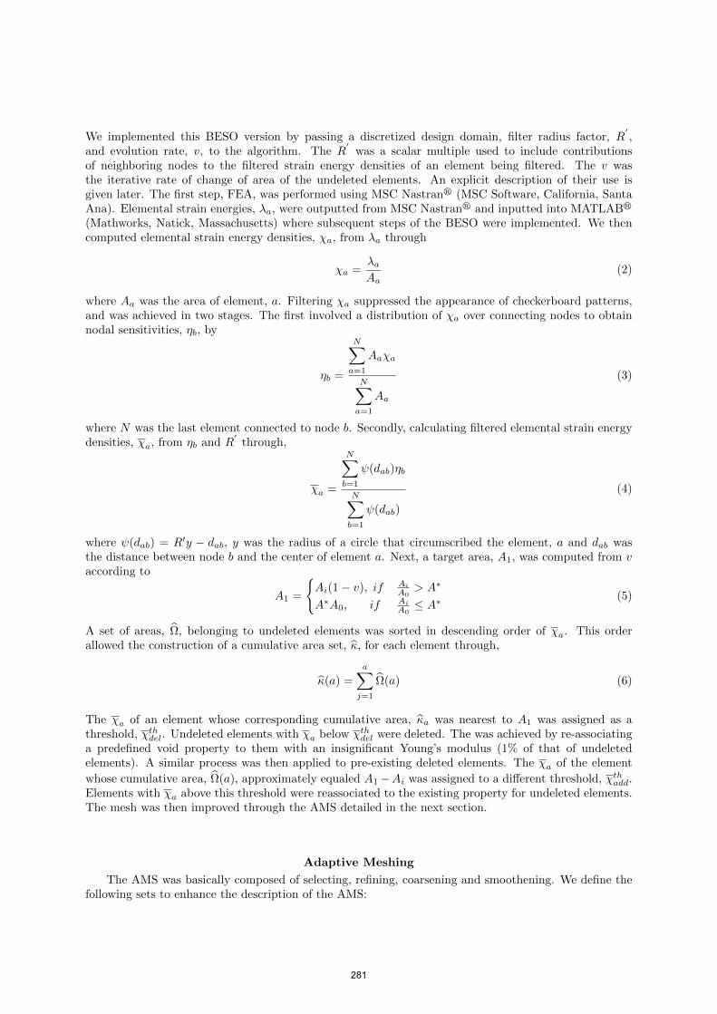
It can be seen that the boundaries of the topologies shown in Figs. 3a and 3c appear darker thanthe interior regions. A magnified view B shown in these Figs. allows a better visualization of the mesh.This is due to the higher density of smaller elements at these boundaries, in contrast to an even shade

284

(a) (b)

(c) (d)

Figure 3: Optima topologies and a magnified view B for (a) Exp.1 (b) Exp. 2 (c) Exp. 3 (d) Exp. 4

observed in Figs. 3b and 3d due to a near constant element size. We characterize each experiment by theCPU time consumed, number of iterations to convergence and the asymptotic strain energy, C∞. Resultsfor these measures are contained in table 1.

Exps. 1 and 2 converged to the same C∞, however Exp. 2 took twice as long as Exp. 1, also requiringa greater number of iterations. A similar trend is repeated for Exp. 3 and Exp. 4, though Exp. 3converged approximately five times faster than Exp. 4. Also while Exp. 1 and 2 attained the same C∞,Exp. 3 and 4 differed slightly. Similarity in C∞ for Exp. 1 and 2 can be attributed to approximately thesame number of nodes at the end of both Exps. as shown in Fig. 4a.

The number of nodes increased in Exp. 1 as the TO progressed to end with a similar number ofnodes to Exp. 2. However, Exp. 3 and Exp. 4 have a significantly different number of nodes at thelast iteration as shown in Fig. 4b. The different number of degrees of freedom makes it difficulty tofairly compare these C∞ values since different levels of FEA errors will exist in the calculation of C.Distortions at the loaded node compound this problem, necessitating a post analysis. Since the mainaim of a strain energy minimization problem is to minimize deflection, the post analysis was performedto determining the stiffness of the topologies. Stiffness in this context refers to the ratio between loadF and the magnitude of a nodal displacement. The chosen node was in the vicinity of the loaded node,however far enough to avoid FEA errors caused by distortion. The location of this node was fixed for alltopologies.

Boundaries of topologies were first extracted, followed by a smoothening process to eliminate therough boundaries without violating V ∗. All, topologies were then remeshed with second order elementsand then analyzed. The number of elements was increased until a converged stiffness, K∞ was reached.The K∞ for the four topologies are shown in table 1. The K∞ for Exp. 1 was slightly greater (0.01%)than that of Exp. 2. Also, K∞ of Exp. 3 was slightly greater (0.001%) than that of Exp. 4. Thissuggested topologies achieved by the AMS were marginally stiffer than those using the BESO algorithm.While it could be argued that the K∞ values of Exp. 1 to 4 were approximately equal, the computationalefficiency offered by the AMS makes it attractive for TO for AM.

285

(a) (b)

Figure 4: Plots of C and nodes against i for (a) Exps. 1 and 2 (b) Exps. 3 and 4

Sensitivity Test

A second set of experiments was performed to compare the sensitivity of the AMS to the startingmesh compared to that of the original BESO. Eight experiments were formulated for this purpose (table2), the first four were performed with the AMS and the second four using the BESO algorithm. TheAmin was set at a low value of 0.001mm2 for the AMS experiments while the initial mesh was populatedwith a different number of elements for the four experiments. The four experiments using the BESOalgorithm had different fixed meshes corresponding to the initial meshes of the AMS experiment. Optimathe topologies for these experiments are shown in Fig. 5. Again, these topologies appear truss-like, notingthat Exps. 11 and 12 correspond to Exps. 2 and 4 respectively.

Table 2: Sensitivity test of AMS and BESO algorithms involving eight experiments (Exps. 5 to 12)characterized by their M , Dmin, Lmin, C∞ and K∞. Standard errors, σm, are also shown.

Exp. Algorithm Start No. elems. Amin M Dmin Lmin C∞ K∞(mm2) (mm) (mm) (mm) (Nmm) (N/mm)

5 AMS 2,000 0.001 28 0.36 0.37 2.25 27.116 AMS 20,000 0.001 26 0.38 0.42 2.29 27.187 AMS 40,000 0.001 31 0.23 0.38 2.31 26.998 AMS 75,000 0.001 28 0.34 0.32 2.30 27.10

σm: 1.03 0.03 0.02 0.049 BESO 2,000 - 10 3.64 10.66 2.09 26.2310 BESO 20,000 - 24 1.66 1.20 2.18 26.7911 BESO 40,000 - 25 0.38 0.38 2.21 26.8412 BESO 75,000 - 35 0.74 0.64 2.23 26.94

σm: 5.14 0.73 2.48 0.32

It was difficult to ascertain the sensitivity of the AMS and the BESO to initial mesh by simple vi-sual inspection of the topologies. Therefore, these topologies were quantified with the number of strutmembers, M , occurring in the optima (table 2), the minimum member thickness, Dmin, the minimummember length, Lmin and K∞. For both the AMS and BESO algorithm, variability in each sample setwas quantified with the standard error in the mean, σm, of these characteristics stated as,

σm =σ√4

(12)

286

(a) (b) (c) (d)

(e) (f) (g) (h)

Figure 5: Optima topologies for (a) Exp. 5 (b) Exp. 6 (c) Exp. 7 (d) Exp. 8 (e) Exp. 9 (f) Exp. 10 (g)Exp. 11 (h) Exp. 12

where σ was the standard deviation of each sample set. The σm for both algorithms can be seen in table2. These values show that there is less variability in the topological data collected for the AMS than withthe BESO algorithm. Secondly, it was observed that the AMS realized members with smaller Dmin andLmin than the BESO. Attaining these dimensions with the BESO, or any other fixed mesh algorithm,would require a much finer mesh, and have high computational time. These finer details are importantas we are now able to produce part with such details via AM. A typical limit of minimum feature size inAM is about 10µm [32]. With regards to C∞, these could not be reliably used to estimate variability inthe performance for the reasons mentioned in the previous section. A useful measure was the standarderror in the K∞, which was also observed to be less for the AMS than that of the BESO as shown in table2. It should also be noted that Figs. 3a and 3b, Figs. 3c and 3d shared similar boundary roughnesssince the size of boundary elements in both sets were largely similar. However, Figs. 3a-3d had smootherboundaries Figs. 3e-3h since elements at their boundaries were much smaller (0.001mm2) than that ofthe uniform meshes used in Figs. 3e-3h. This demonstrates that the AMS is able to achieve smootherboundaries than the BESO algorithm at a lower computation cost.

Conclusion and further work

A hybrid TO algorithm is proposed constituted by a modified form of the BESO algorithm andan adaptive meshing strategy (AMS). The BESO algorithm was modified so that it was based on strainenergy densities since the AMS caused a progressive variation in elemental sizes. A two dimensional plateproblem was solved to benchmark performance of the hybrid against that of the BESO algorithm. TheAMS was found to be substantially more efficient, with a reduction in computation time of 52% and 82%respectively for the cases investigated, with similar performance. It was also less sensitive to the startingmesh and able to attain smoother boundaries with a lower number of elements. Also, finer featuresare achievable with the AMS, starting with relatively coarse meshes. This is particularly interesting fortopologies to be made via additive manufacture (AM). Since AM can achieve parts with high degrees ofcomplexity. Further work could involve the determination of an element size that corresponds to AM’sresolution. Also, the AMS could be extended to practical three dimensional parts experiencing single andmultiple load cases.

Acknowledgements

The authors are grateful for the funding provided by the IMCRC and EPSRC.

287

References

[1] Mitchell, A.G.M., The limits of economy in frame structures, Philo, Mag. Sec, 6(8), p.589-597 (1904).

[2] Rozvany, G.I.N., Aims, scope, methods, history, and unified terminology of computer-aided topologicaloptimization in structural mechanics. Struct Multidisc Optim, 21, p. 19 (2001).

[3] Kirsh, U., On optimal topologies of grillage structures, Engineering with computers, 42(8), p.223-239(1986).

[4] Bendsoe, M.P., Kikuchi, Generating optimal topologies in structural design using a homogenizationmethod. Computer Methods in Applied Mechanics and Engineering, 71, p. 28 (1988).

[5] Rozvany, G., I., N., Zhou, M., Birker, T., Generalized shape optimization without homogenization,Structural Optimization, 4, p.250-252 (1992).

[6] Xie, Y., M., Steven, G.P., Evolutionary Structural Optimization, 188p., Springer-Verlag, London(1997).

[7] Zhou, M., Rozvany, G.I.N., On the validity of ESO type methods in topological optimization. StructMultidisc Optim, 21, p. 4 (2001).

[8] Mattheck, C., Burkhardt, S., Erb, D., Shape optimization of engineering components by adaptivebiological growth. In: Eschenauer, H., A.; Mattheck, C.; Olhoof, N. (eds) Engineering optimization indesign processes, pp.15-26. Berlin, Heidelberg, New York, Springer, 1991.

[9] Querin, O., M., Young, V., Steven, G., P., Xie, Y., M., Computational Efficiency and validation ofbi-directional evolutionary structural optimization, Comput Methods Applied Mechanical Engineering,189, p.559-573 (2000b).

[10] Huang, X., Xie, Y., M., Convergent and mesh-independent solutions for the bi-directional evolution-ary structural optimization method, Finite Elements in Analysis and Design, 43, p.1039-1040 (2007).

[11] Sandgren, E., Jensen, E., Welton, J., Topological design of structural components using geneticoptimization methods, in Sensitivity Analysis and Optimization with Numerical Methods, S. Saigal andS. Mukherjee, eds., Proceedings of the Winter Annual Meeting of the American Society of MechanicalEngineers 115, pp. 31(43), Texas, 1990.

[12] Chapman, C., D., Saitou, K., Jakiela, M., J., Genetic algorithms as an approach to configurationand topology design, Journal of Mechanical Design, 116(105), 8p. (1994).

[13] Chapman, C., D., Jakiela, M., J., Genetic algorithm-based structural topology design with complianceand topology simplification consideration, Journal of Mechanical Design 118(89), 10p. (1996).

[14] Kaveh, A., Hassani, B., Shojaee, S., Tavakkoli, S., M., Structural topology optimization using antcolony methodology, Engineering Structures, 30, p.2559-2566 (2008).

[15] Luh, G., Lin, C., Structural topology optimization using ant colony optimization algorithm, AppliedSoft Computing, 9, p.1343-1353 (2009).

[16] Luh, G., Lin, C., Lin, Y., A binary particle swarm optimization for continuum using topology opti-mization, Applied Soft Computing, 11, p.2833-2844 (2011).

[17] Bureerat, S., Limtragool, J., Structural topology optimization using simulated annealing with mul-tiresolution design variables, Finite Elements in Analysis and Design, 44, p.738-747 (2008).

[18] Zuo, Z.H., Xie, Y.M., Huang X., Combining genetic algorithms with BESO for topology optimization.Struct Multidisc Optim, 38, p. 13, (2009).

288

[19] Garcia-Lopez, N., P., Sanchez-Silva, M., Medaglia, A., L., Chateauneuf, A., An improved hybridtopology optimization approach coupling simulated annealing and SIMP, IOP Conf. Series: MaterialsScience and Engineering, 10, WCCM/APCOM, (2010).

[20] Heubner, K., H., Dewhirst, D., L., Smith, D., E., Byrom, T., G., The finite element method forengineers, John Wiley and Sons, 4th ed, New York, (2001).

[21] Kuo, Y., L., Cleghorn, W., L., Behdinan, K., Fenton, R., G., The h-p-r-refinement finite elementanalysis of a planar high-speed four-bar mechanism, Mechanism and Machine Theory, 41, p.505-524(2006).

[22] Kim, H., Garcia, M., J., Querin, O., M., Steven, J., P., Xie, Y., M., Introduction of fixed grid inevolutionary structural optimization, Engineering Computation, 17(4), p.427-439 (2000).

[23] Mariano, V., Marti, P., M., Querin, O., M., Topology design of two-dimensional continuum structuresusing isolines, Computer and Structures, 87, p.101-109 (2009).

[24] Gibson, I., Rosen, D., W., Stucker, B., Additive Manufacturing Technologies, 459p., Springer, NewYork (2009).

[25] Tuck, C.J., Hague, R., J., M., Ruffo, M., Ransley, M., Adams, P., Rapid manufacturing facilitatedcustomization, International Journal of Computer Integrated Manufacturing, 21(3), p.245-258 (2008).

[26] Hague, R., Mansour, S., Saleh N., Design opportunities with rapid manufacturing, Assembly Au-tomation, 23(4), p.346-356 (2003).

[27] Rosen, D., W., Computer-Aided design for additive manufacturing of cellular structures, Computer-Aided design and applications, 4(5), p.585-594 (2007).

[28] Engwirda, D., Unstructured Mesh Methods for the Navier Stokes Equations, Undergraduate thesis,The school of Aerospace Engineerinf, The University of Sydney, 2005.

[29] Bhatia, R., P., Lawrence, K., L., Two-dimensional finite element mesh generation based on stripwaiseautomatic triangulation, Computer and structures, 36, p.309-319 (1990.)

[30] Zhigeng, P., Kun, Z., Jiaoying, S., A New mesh simplification algorithm based on triangle collapses,16(1), p.8 (2001).

[31] Glen, A., Hansen, R., W., Douglas, A., Z., Mesh enhancement: Selected elliptic methods, foundationsand applications, Imperial College Press, 515p., London, 2005.

[32] Cohen, A., Chen, R., Frodis, U., Wu, M., Folk, C., Microscale metal additive manufacturing ofmulti-component medical devices, Rapid Prototyping Journal, 16(3), p.209-215 (2010).

289