energies

Conference Report

Hybrid, Multi-Megawatt HVDC TransformerTopology Comparison for Future OffshoreWind Farms

Michael Smailes 1,* , Chong Ng 1, Paul Mckeever 1, Jonathan Shek 2, Gerasimos Theotokatos 3

and Mohammad Abusara 4

1 Research and Disruptive Innovation, Offshore Renewable Energy Catapult (ORE Catapult),Blyth NE24 1LZ, UK; chong.ng@ore.catapult.org.uk (C.N.); Paul.Mckeever@ore.catapult.org.uk (P.M.)

2 Institute for Energy Systems, Edinburgh University, Edinburgh EH8 9YL, UK; J.Shek@ed.ac.uk3 Naval Architecture, Ocean & Marine, Strathclyde University, Glasgow G1 1XW, UK;

gerasimos.theotokatos@strath.ac.uk4 Renewable Energy, Exeter University, Exeter EX4 4SB, UK; M.Abusara@exeter.ac.uk* Correspondence: m.smailes@ed.ac.uk or Michael.Smailes@ORE.Catapult.org.uk; Tel.: +44-(0)1670-54-3008

Academic Editor: Simon WatsonReceived: 24 March 2017; Accepted: 13 June 2017; Published: 27 June 2017

Abstract: With the wind industry moving further offshore, High Voltage Direct Current (HVDC)transmission is becoming increasingly popular. HVDC transformer substations are not optimizedfor the offshore industry though, increasing costs and reducing redundancy. A suggested mediumfrequency, modular hybrid HVDC transformer located within each wind turbine nacelle couldmitigate these problems, but the overall design must be considered carefully to minimize losses.This paper’s contribution is a detailed analysis of the hybrid transformer, using practical designconsiderations including component library minimization. The configurations investigated includecombinations of single phase H-Bridge and Modular Multilevel Converter topologies operating underminimum switching frequency control strategies. These were modelled in the MATLAB/Simulinkenvironment. The impact of the minimum switching control strategy and converter topology onpower transfer stability and overall efficiency is then investigated. It was found that the H-Bridgeconverter generated the lowest overall losses, but there was a trade off with power flow sensitivitydue in part to the additional harmonics generated.

Keywords: high voltage direct current; power converters; transformer loss; improved generalSteinmetz equation; Steinmetz equation; wind energy; power transmission

1. Introduction

Over the last decade, the average distance to shore for new wind farms has increased to exploitthe higher and more consistent wind conditions, resulting in more High Voltage Direct Current(HVDC) connected wind farms [1,2]. The HVDC substation designs used to date are ill-suited for theoffshore environment though. Based on their onshore counterparts, they offer little redundancy andaccount for 12% of a wind farm’s capital costs [3–5], most of which is attributed to the structural andinstallation costs. To address this, a concept was introduced in [6] to eliminate the offshore substationby modularizing and miniaturizing the electrical equipment to fit within the turbines themselves.This hybrid HVDC transformer was investigated as part of a conference paper in [7], and is nowfurther expanded in this article. As the hybrid HVDC transformer is located within each turbine, theturbines themselves are connected in parallel directly to a HVDC collection grid (Figure 1). The HVDCsubstations are therefore not required, and the system redundancy is improved. To accommodate the

Energies 2017, 10, 851; doi:10.3390/en10070851 www.mdpi.com/journal/energies

Energies 2017, 10, 851 2 of 15

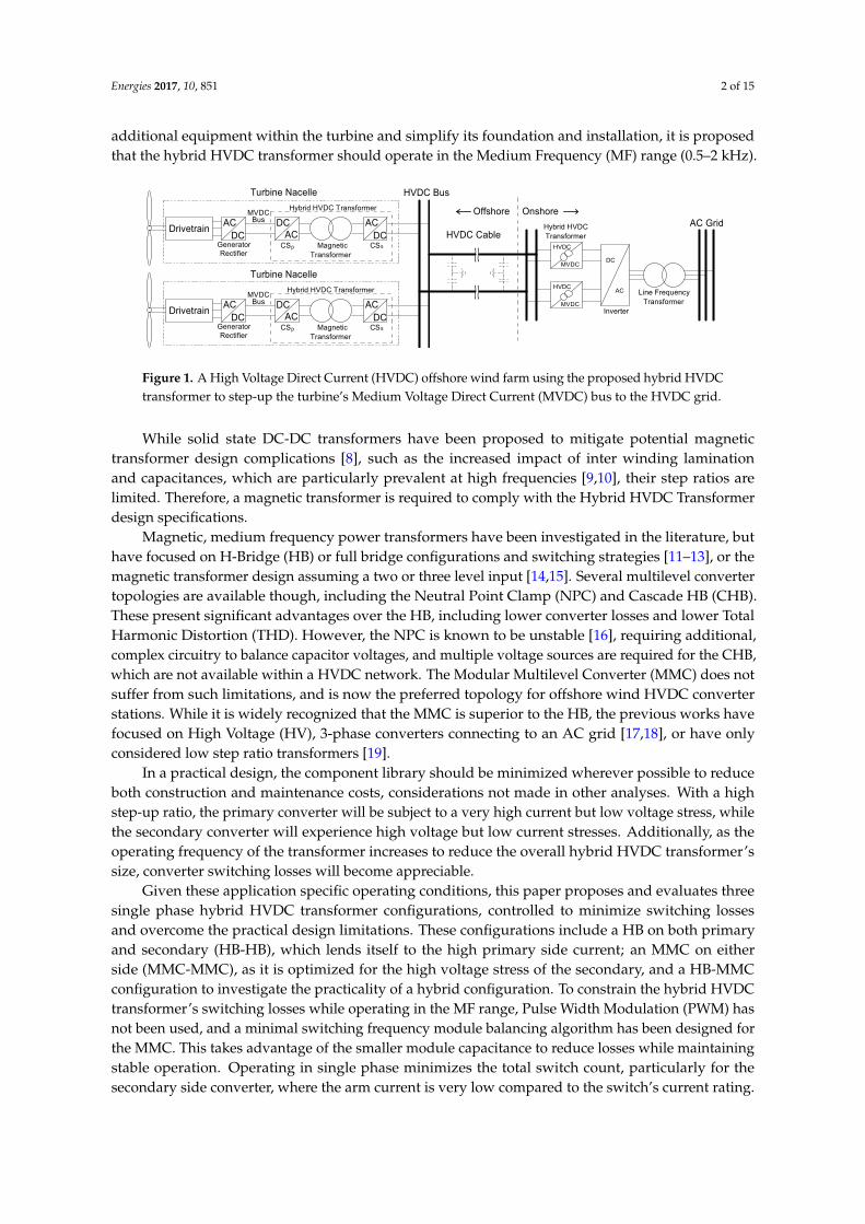
additional equipment within the turbine and simplify its foundation and installation, it is proposedthat the hybrid HVDC transformer should operate in the Medium Frequency (MF) range (0.5–2 kHz).

Energies 2017, 10, 851 2 of 15

installation, it is proposed that the hybrid HVDC transformer should operate in the Medium Frequency (MF) range (0.5–2 kHz).

While solid state DC-DC transformers have been proposed to mitigate potential magnetic transformer design complications [8], such as the increased impact of inter winding lamination and capacitances, which are particularly prevalent at high frequencies [9,10], their step ratios are limited. Therefore, a magnetic transformer is required to comply with the Hybrid HVDC Transformer design specifications.

Figure 1. A High Voltage Direct Current (HVDC) offshore wind farm using the proposed hybrid HVDC transformer to step-up the turbine’s Medium Voltage Direct Current (MVDC) bus to the HVDC grid.

Magnetic, medium frequency power transformers have been investigated in the literature, but have focused on H-Bridge (HB) or full bridge configurations and switching strategies [11–13], or the magnetic transformer design assuming a two or three level input [14,15]. Several multilevel converter topologies are available though, including the Neutral Point Clamp (NPC) and Cascade HB (CHB). These present significant advantages over the HB, including lower converter losses and lower Total Harmonic Distortion (THD). However, the NPC is known to be unstable [16], requiring additional, complex circuitry to balance capacitor voltages, and multiple voltage sources are required for the CHB, which are not available within a HVDC network. The Modular Multilevel Converter (MMC) does not suffer from such limitations, and is now the preferred topology for offshore wind HVDC converter stations. While it is widely recognized that the MMC is superior to the HB, the previous works have focused on High Voltage (HV), 3-phase converters connecting to an AC grid [17,18], or have only considered low step ratio transformers [19].

In a practical design, the component library should be minimized wherever possible to reduce both construction and maintenance costs, considerations not made in other analyses. With a high step-up ratio, the primary converter will be subject to a very high current but low voltage stress, while the secondary converter will experience high voltage but low current stresses. Additionally, as the operating frequency of the transformer increases to reduce the overall hybrid HVDC transformer’s size, converter switching losses will become appreciable.

Given these application specific operating conditions, this paper proposes and evaluates three single phase hybrid HVDC transformer configurations, controlled to minimize switching losses and overcome the practical design limitations. These configurations include a HB on both primary and secondary (HB-HB), which lends itself to the high primary side current; an MMC on either side (MMC-MMC), as it is optimized for the high voltage stress of the secondary, and a HB-MMC configuration to investigate the practicality of a hybrid configuration. To constrain the hybrid HVDC transformer’s switching losses while operating in the MF range, Pulse Width Modulation (PWM) has not been used, and a minimal switching frequency module balancing algorithm has been designed for the MMC. This takes advantage of the smaller module capacitance to reduce losses while maintaining stable operation. Operating in single phase minimizes the total switch count, particularly for the secondary side converter, where the arm current is very low compared to the switch’s current rating.

ACDC

DrivetrainAC

DCAC

DC

HVDC Bus

Hybrid HVDC Transformer

DrivetrainAC

DC

CS CSMagneticTransformer

ACDC AC

DCMagnetic

Transformer

p s

Turbine Nacelle

Turbine Nacelle

HVDC Cable

∼ ∼∼ ∼

HVDC

MVDC

HVDC

MVDC

DC

AC

Hybrid HVDC

Hybrid HVDC Transformer

Transformer

Line FrequencyTransformer

AC Grid

Inverter

MVDCBus

MVDCBus

GeneratorRectifier

GeneratorRectifier

CSp CSs

Offshore Onshore

Figure 1. A High Voltage Direct Current (HVDC) offshore wind farm using the proposed hybrid HVDCtransformer to step-up the turbine’s Medium Voltage Direct Current (MVDC) bus to the HVDC grid.

While solid state DC-DC transformers have been proposed to mitigate potential magnetictransformer design complications [8], such as the increased impact of inter winding laminationand capacitances, which are particularly prevalent at high frequencies [9,10], their step ratios arelimited. Therefore, a magnetic transformer is required to comply with the Hybrid HVDC Transformerdesign specifications.

Magnetic, medium frequency power transformers have been investigated in the literature, buthave focused on H-Bridge (HB) or full bridge configurations and switching strategies [11–13], or themagnetic transformer design assuming a two or three level input [14,15]. Several multilevel convertertopologies are available though, including the Neutral Point Clamp (NPC) and Cascade HB (CHB).These present significant advantages over the HB, including lower converter losses and lower TotalHarmonic Distortion (THD). However, the NPC is known to be unstable [16], requiring additional,complex circuitry to balance capacitor voltages, and multiple voltage sources are required for the CHB,which are not available within a HVDC network. The Modular Multilevel Converter (MMC) does notsuffer from such limitations, and is now the preferred topology for offshore wind HVDC converterstations. While it is widely recognized that the MMC is superior to the HB, the previous works havefocused on High Voltage (HV), 3-phase converters connecting to an AC grid [17,18], or have onlyconsidered low step ratio transformers [19].

In a practical design, the component library should be minimized wherever possible to reduceboth construction and maintenance costs, considerations not made in other analyses. With a highstep-up ratio, the primary converter will be subject to a very high current but low voltage stress, whilethe secondary converter will experience high voltage but low current stresses. Additionally, as theoperating frequency of the transformer increases to reduce the overall hybrid HVDC transformer’ssize, converter switching losses will become appreciable.

Given these application specific operating conditions, this paper proposes and evaluates threesingle phase hybrid HVDC transformer configurations, controlled to minimize switching lossesand overcome the practical design limitations. These configurations include a HB on both primaryand secondary (HB-HB), which lends itself to the high primary side current; an MMC on eitherside (MMC-MMC), as it is optimized for the high voltage stress of the secondary, and a HB-MMCconfiguration to investigate the practicality of a hybrid configuration. To constrain the hybrid HVDCtransformer’s switching losses while operating in the MF range, Pulse Width Modulation (PWM) hasnot been used, and a minimal switching frequency module balancing algorithm has been designed forthe MMC. This takes advantage of the smaller module capacitance to reduce losses while maintainingstable operation. Operating in single phase minimizes the total switch count, particularly for thesecondary side converter, where the arm current is very low compared to the switch’s current rating.

Energies 2017, 10, 851 3 of 15

This paper’s contribution is the detailed evaluation of the HB-HB, MMC-MMC, and HB-MMCconfigurations using simulations in the MATLAB/Simulink environment. These simulations are usedto calculate their conduction, switching, and transformer core loss at operating frequencies rangingfrom 0.5 to 2 kHz. The magnetic transformer design and winding losses are not considered here forbrevity however, as they have been calculated in [20]. Furthermore, the ability for each configurationto maintain stable power transfer over the tested frequency range is considered. This will revealcontrol stability concerns relating to the HB-HB and HB-MMC configurations and inefficiencies inthe MMC-MMC case, primarily due to the primary side converter. This will impact on the designconsiderations for MF transformer design, particularly on the tradeoff between losses and powertransfer stability.

The rest of the paper is structured as follows. The MATLAB/Simulink models are described inSection 2. The converter and magnetic transformer loss calculations carried out on the waveformsgenerated by the computer modules are detailed in Section 3, and the results presented in Section 4.These results are discussed in detail in Section 5, and a conclusion is drawn in Section 6.

2. Computer Simulation

2.1. Simulation Models

The models were arbitrarily designed for a 6.5 MW wind turbine with a nominal 6 kV MediumVoltage Direct Current (MVDC) bus voltage (vin) between the fully rated generator rectifier andhybrid transformer (Figure 1). Steady state operation at the rated power was assumed throughout thesimulations with the generator rectifier allowing a variable speed turbine operation. The transformeroutput connects to a ±300 kV HVDC via a shunt connection.

The model used to evaluate the performance of each transformer configuration is shown ingeneric form in Figure 2, and the converter topologies are shown in Figure 3. In the model, the HVDCbus is assumed to be constant and is modelled using a DC voltage source. In modern wind turbines,the MVDC bus voltage is variable to allow the grid side converter to control reactive power flow.This is reflected in the model by a constant and variable DC voltage source in series, managed by theprimary side converter control. The control of the output real power (Pout) and reactive power (QT) aregoverned by the algorithms shown in Figure 4, where voltage (vp) and current (ip) inputs are taken atthe locations shown in Figure 2. The primary and secondary DC bus resistances are embodied by Rp

and Rs respectively, and the magnetic transformer has a turns ratio of 1:100. It is known that the powertransferred through the transformer (PT) is given by (1) for a primary and referred secondary voltage(vp and vs

′ respectively), transformer reactance (XT), and load angle (δ).

PT =vpvs

′ sin(δ)XT

(1)

Since vp and vs′ are fixed by the turbine specifications, the δ range is determined by the transformer

inductance (LT) and should be selected to maintain stable control and allow 6.5 MW to be transferred.Moreover, LT was designed to prevent high frequency voltage harmonics generated by switchingevents from showing in the arm current and magnetic flux waveforms, and hence prevent coresaturation. With these considerations, LT lumped on the primary side was chosen to be 0.1 mH.

Energies 2017, 10, 851 4 of 15Energies 2017, 10, 851 4 of 15

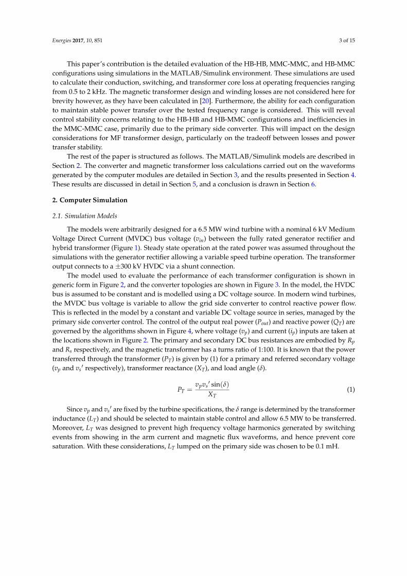
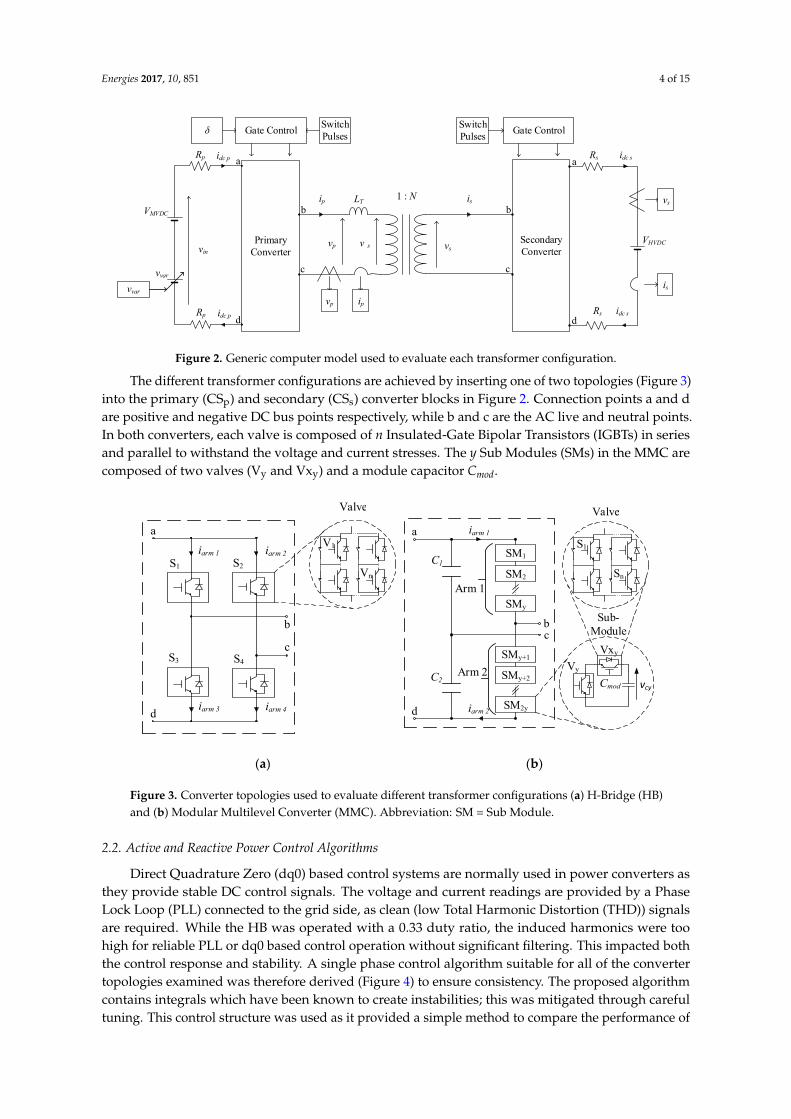
Figure 2. Generic computer model used to evaluate each transformer configuration.

The different transformer configurations are achieved by inserting one of two topologies (Figure 3) into the primary (CSp) and secondary (CSs) converter blocks in Figure 2. Connection points a and d are positive and negative DC bus points respectively, while b and c are the AC live and neutral points. In both converters, each valve is composed of n Insulated-Gate Bipolar Transistors (IGBTs) in series and parallel to withstand the voltage and current stresses. The y Sub Modules (SMs) in the MMC are composed of two valves (Vy and Vxy) and a module capacitor Cmod.

(a) (b)

Figure 3. Converter topologies used to evaluate different transformer configurations (a) H-Bridge (HB) and (b) Modular Multilevel Converter (MMC). Abbreviation: SM = Sub Module.

2.2. Active and Reactive Power Control Algorithms

Direct Quadrature Zero (dq0) based control systems are normally used in power converters as they provide stable DC control signals. The voltage and current readings are provided by a Phase Lock Loop (PLL) connected to the grid side, as clean (low Total Harmonic Distortion (THD)) signals are required. While the HB was operated with a 0.33 duty ratio, the induced harmonics were too high for reliable PLL or dq0 based control operation without significant filtering. This impacted both the control response and stability. A single phase control algorithm suitable for all of the converter topologies examined was therefore derived (Figure 4) to ensure consistency. The proposed algorithm contains integrals which have been known to create instabilities; this was mitigated through careful tuning. This control structure was used as it provided a simple method to compare the performance

Rp idc p

Rp idc p

VMVDC

vvar

vvar

vin

Primary Converter

a

d

Gate Control Switch Pulsesδ

LT

vp ip

1 : Nip

vs

b

c

Secondary Converter

is

b

c

a

d

VHVDC

Rs idc s

Rs

vs

is

idc s

Gate ControlSwitch Pulses

vp v s

S2

S3 S4

iarm 1 iarm 2

b

c

V1

Vn

iarm 3 iarm 4

a

d

S1

Valve

vcy

Vxy

Vy

Cmod

SM2

SMy

SMy+2

SMy+1

SM2y

SM1

bc

a

d

iarm 1

iarm 2

C1

C2

Arm 1

Arm 2

S1

Sn

Valve

Sub-Module

Figure 2. Generic computer model used to evaluate each transformer configuration.

The different transformer configurations are achieved by inserting one of two topologies (Figure 3)into the primary (CSp) and secondary (CSs) converter blocks in Figure 2. Connection points a and dare positive and negative DC bus points respectively, while b and c are the AC live and neutral points.In both converters, each valve is composed of n Insulated-Gate Bipolar Transistors (IGBTs) in seriesand parallel to withstand the voltage and current stresses. The y Sub Modules (SMs) in the MMC arecomposed of two valves (Vy and Vxy) and a module capacitor Cmod.

Energies 2017, 10, 851 4 of 15

Figure 2. Generic computer model used to evaluate each transformer configuration.

The different transformer configurations are achieved by inserting one of two topologies (Figure 3) into the primary (CSp) and secondary (CSs) converter blocks in Figure 2. Connection points a and d are positive and negative DC bus points respectively, while b and c are the AC live and neutral points. In both converters, each valve is composed of n Insulated-Gate Bipolar Transistors (IGBTs) in series and parallel to withstand the voltage and current stresses. The y Sub Modules (SMs) in the MMC are composed of two valves (Vy and Vxy) and a module capacitor Cmod.

(a) (b)

Figure 3. Converter topologies used to evaluate different transformer configurations (a) H-Bridge (HB) and (b) Modular Multilevel Converter (MMC). Abbreviation: SM = Sub Module.

2.2. Active and Reactive Power Control Algorithms

Direct Quadrature Zero (dq0) based control systems are normally used in power converters as they provide stable DC control signals. The voltage and current readings are provided by a Phase Lock Loop (PLL) connected to the grid side, as clean (low Total Harmonic Distortion (THD)) signals are required. While the HB was operated with a 0.33 duty ratio, the induced harmonics were too high for reliable PLL or dq0 based control operation without significant filtering. This impacted both the control response and stability. A single phase control algorithm suitable for all of the converter topologies examined was therefore derived (Figure 4) to ensure consistency. The proposed algorithm contains integrals which have been known to create instabilities; this was mitigated through careful tuning. This control structure was used as it provided a simple method to compare the performance

Rp idc p

Rp idc p

VMVDC

vvar

vvar

vin

Primary Converter

a

d

Gate Control Switch Pulsesδ

LT

vp ip

1 : Nip

vs

b

c

Secondary Converter

is

b

c

a

d

VHVDC

Rs idc s

Rs

vs

is

idc s

Gate ControlSwitch Pulses

vp v s

S2

S3 S4

iarm 1 iarm 2

b

c

V1

Vn

iarm 3 iarm 4

a

d

S1

Valve

vcy

Vxy

Vy

Cmod

SM2

SMy

SMy+2

SMy+1

SM2y

SM1

bc

a

d

iarm 1

iarm 2

C1

C2

Arm 1

Arm 2

S1

Sn

Valve

Sub-Module

Figure 3. Converter topologies used to evaluate different transformer configurations (a) H-Bridge (HB)and (b) Modular Multilevel Converter (MMC). Abbreviation: SM = Sub Module.

2.2. Active and Reactive Power Control Algorithms

Direct Quadrature Zero (dq0) based control systems are normally used in power converters asthey provide stable DC control signals. The voltage and current readings are provided by a PhaseLock Loop (PLL) connected to the grid side, as clean (low Total Harmonic Distortion (THD)) signalsare required. While the HB was operated with a 0.33 duty ratio, the induced harmonics were toohigh for reliable PLL or dq0 based control operation without significant filtering. This impacted boththe control response and stability. A single phase control algorithm suitable for all of the convertertopologies examined was therefore derived (Figure 4) to ensure consistency. The proposed algorithmcontains integrals which have been known to create instabilities; this was mitigated through carefultuning. This control structure was used as it provided a simple method to compare the performance of

Energies 2017, 10, 851 5 of 15

each converter topology, and while it is included for reference, the focus of this paper is the converter’sperformance and not its control.

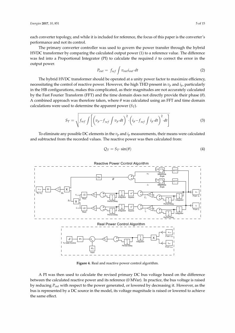
The primary converter controller was used to govern the power transfer through the hybridHVDC transformer by comparing the calculated output power (1) to a reference value. The differencewas fed into a Proportional Integrator (PI) to calculate the required δ to correct the error in theoutput power.

Pout = fre f

∫voutiout·dt (2)

The hybrid HVDC transformer should be operated at a unity power factor to maximize efficiency,necessitating the control of reactive power. However, the high THD present in vp and ip, particularlyin the HB configurations, makes this complicated, as their magnitudes are not accurately calculatedby the Fast Fourier Transform (FFT) and the time domain does not directly provide their phase (θ).A combined approach was therefore taken, where θ was calculated using an FFT and time domaincalculations were used to determine the apparent power (ST).

ST =

√√√√ fre f

∫ [(vp− f re f

∫vp·dt

)2·(

ip− f re f

∫ip·dt

)2·dt

](3)

To eliminate any possible DC elements in the vp and ip measurements, their means were calculatedand subtracted from the recorded values. The reactive power was then calculated from:

QT = ST · sin(θ) (4)

Energies 2017, 10, 851 5 of 15

of each converter topology, and while it is included for reference, the focus of this paper is the converter’s performance and not its control.

The primary converter controller was used to govern the power transfer through the hybrid HVDC transformer by comparing the calculated output power (1) to a reference value. The difference was fed into a Proportional Integrator (PI) to calculate the required δ to correct the error in the output power. = ∙ (2)

The hybrid HVDC transformer should be operated at a unity power factor to maximize efficiency, necessitating the control of reactive power. However, the high THD present in vp and ip, particularly in the HB configurations, makes this complicated, as their magnitudes are not accurately calculated by the Fast Fourier Transform (FFT) and the time domain does not directly provide their phase (θ). A combined approach was therefore taken, where θ was calculated using an FFT and time domain calculations were used to determine the apparent power (ST).

ST= fref vp-fref

vp·dt2

· ip-fref ip·dt2

·dt (3)

To eliminate any possible DC elements in the vp and ip measurements, their means were calculated and subtracted from the recorded values. The reactive power was then calculated from: = ∙ sin( ) (4)

Figure 4. Real and reactive power control algorithm.

A PI was then used to calculate the revised primary DC bus voltage based on the difference between the calculated reactive power and its reference (0 MVar). In practice, the bus voltage is raised by reducing Pout with respect to the power generated, or lowered by decreasing it. However, as the bus is represented by a DC source in the model, its voltage magnitude is raised or lowered to achieve the same effect.

2.3. MMC Control Algorithm

Sin

i

vv

i

Sp

p

p rms

p rms

v

i

θ

θ

θ

Q p

p

_

_

Integrator

MagnitudeAngle

SquareRoot

-1

f ref

f ref

fref

fref

Integrator

Integrator

Square

MagnitudeAngle

Root

Integrator

v p

ip

From p

From p

v var

f ref

Period Delay

Integratorδ

Pref

Input

v out

Iout

out

From out

To Gate Control

Real Power Control Algorithm

Reactive Power Control Algorithm

FFT

FFT

}u

u-

| | --/_

}u

u-

| | --/_

+-

+-

+-

s1_

s1_

s1_

s1_

u2

u2

z1_

z1_

z1_

z1_

+-

+-

u\/_

u\/_

X

XPI

+-

+-

z1_

+-+-PI s

1_ X

To var

Period Delay

Period Delay

Period Delay

Period Delay

v

i

v

From v

v

Figure 4. Real and reactive power control algorithm.

A PI was then used to calculate the revised primary DC bus voltage based on the differencebetween the calculated reactive power and its reference (0 MVar). In practice, the bus voltage is raisedby reducing Pout with respect to the power generated, or lowered by decreasing it. However, as thebus is represented by a DC source in the model, its voltage magnitude is raised or lowered to achievethe same effect.

Energies 2017, 10, 851 6 of 15

2.3. MMC Control Algorithm

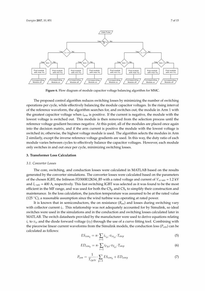
While the same algorithms used for the HB are used to control P and Q, the MMC requires amore complex switching algorithm to balance the module capacitor voltages (vc). Depending on thedirection of the arm current (iarm), the module capacitors will either charge or discharge when theyare switched in or placed in the current path. Modules are switched in when Sxy is conducting andbypassed when Sy is conducting to create the desired voltage steps. Sxy and Sy must never bothconduct though, or the module capacitor will be short-circuited. Multiple module combinations arepossible for each voltage level, apart from the maximum and minimum voltage level (Figure 5).

Energies 2017, 10, 851 6 of 15

While the same algorithms used for the HB are used to control P and Q, the MMC requires a more complex switching algorithm to balance the module capacitor voltages (vc). Depending on the direction of the arm current (iarm), the module capacitors will either charge or discharge when they are switched in or placed in the current path. Modules are switched in when Sxy is conducting and bypassed when Sy is conducting to create the desired voltage steps. Sxy and Sy must never both conduct though, or the module capacitor will be short-circuited. Multiple module combinations are possible for each voltage level, apart from the maximum and minimum voltage level (Figure 5).

An algorithm can therefore be devised to provide the desired output voltage waveform while balancing the module capacitor voltages, such that each remains at the average voltage. This algorithm determines the switching strategy of the converter, and hence directly influences the switching losses and quality of the AC and DC waveforms. Algorithms utilizing PWM have been suggested in the literature [21] to improve capacitor voltage balancing, as the instantaneous duty of each module is reduced. The module capacitor voltage remains closer to the average module voltage and DC ripple is minimized. However, this will increase the switching frequency of the converter and increase losses.

As the converters analyzed here are to operate in the MF range, the switching losses for PWM would be too great. That said, the higher switching frequency also reduces the effect of the DC ripple. An alternative control algorithm (Figure 6) has therefore been developed, taking advantage of the reduced DC ripple for the purposes of this study.

Figure 5. Switching pattern for a 3L MMC.

Figure 6. Flow diagram of module capacitor voltage balancing algorithm for MMC.

Valve Logic

S1 1 1 1 0 1 0 1 0 0 0

S2 0 1 0 0 0 1 1 1 0 1

S3 1 0 1 1 1 0 0 0 1 0

S4 0 0 0 1 0 1 0 1 1 1

S1x 0 1 0 0 0 1 1 1 0 1

S2x 1 1 1 0 1 0 1 0 0 0

S3x 0 0 0 1 0 1 0 1 1 1

S4x 1 0 1 1 1 0 0 0 1 0

1

0

-1

Gate Pulse

dadt_ >0

iarm > 0

Arm 1

Find module Find modulewith max V with min Vcy cy

Arm 1

Find modulewith max Vcy

Find modulewith min Vcy

Yes No NoYes

Corresponding CorrespondingModule off Module on

CorrespondingModule off

CorrespondingModule on

Yes No

Yes

iarm > 0

Arm 1

Find module Find modulewith min V with max Vcy cy

Arm 1

Find modulewith min Vcy

Find modulewith max Vcy

Yes No NoYes

Corresponding CorrespondingModule on Module off

CorrespondingModule on

CorrespondingModule off

Yes No

Noref

Figure 5. Switching pattern for a 3L MMC.

An algorithm can therefore be devised to provide the desired output voltage waveform whilebalancing the module capacitor voltages, such that each remains at the average voltage. This algorithmdetermines the switching strategy of the converter, and hence directly influences the switching lossesand quality of the AC and DC waveforms. Algorithms utilizing PWM have been suggested in theliterature [21] to improve capacitor voltage balancing, as the instantaneous duty of each module isreduced. The module capacitor voltage remains closer to the average module voltage and DC ripple isminimized. However, this will increase the switching frequency of the converter and increase losses.

As the converters analyzed here are to operate in the MF range, the switching losses for PWMwould be too great. That said, the higher switching frequency also reduces the effect of the DC ripple.An alternative control algorithm (Figure 6) has therefore been developed, taking advantage of thereduced DC ripple for the purposes of this study.

Energies 2017, 10, 851 7 of 15

Energies 2017, 10, 851 6 of 15

While the same algorithms used for the HB are used to control P and Q, the MMC requires a more complex switching algorithm to balance the module capacitor voltages (vc). Depending on the direction of the arm current (iarm), the module capacitors will either charge or discharge when they are switched in or placed in the current path. Modules are switched in when Sxy is conducting and bypassed when Sy is conducting to create the desired voltage steps. Sxy and Sy must never both conduct though, or the module capacitor will be short-circuited. Multiple module combinations are possible for each voltage level, apart from the maximum and minimum voltage level (Figure 5).

An algorithm can therefore be devised to provide the desired output voltage waveform while balancing the module capacitor voltages, such that each remains at the average voltage. This algorithm determines the switching strategy of the converter, and hence directly influences the switching losses and quality of the AC and DC waveforms. Algorithms utilizing PWM have been suggested in the literature [21] to improve capacitor voltage balancing, as the instantaneous duty of each module is reduced. The module capacitor voltage remains closer to the average module voltage and DC ripple is minimized. However, this will increase the switching frequency of the converter and increase losses.

As the converters analyzed here are to operate in the MF range, the switching losses for PWM would be too great. That said, the higher switching frequency also reduces the effect of the DC ripple. An alternative control algorithm (Figure 6) has therefore been developed, taking advantage of the reduced DC ripple for the purposes of this study.

Figure 5. Switching pattern for a 3L MMC.

Figure 6. Flow diagram of module capacitor voltage balancing algorithm for MMC.

Valve Logic

S1 1 1 1 0 1 0 1 0 0 0

S2 0 1 0 0 0 1 1 1 0 1

S3 1 0 1 1 1 0 0 0 1 0

S4 0 0 0 1 0 1 0 1 1 1

S1x 0 1 0 0 0 1 1 1 0 1

S2x 1 1 1 0 1 0 1 0 0 0

S3x 0 0 0 1 0 1 0 1 1 1

S4x 1 0 1 1 1 0 0 0 1 0

1

0

-1

Gate Pulse

dadt_ >0

iarm > 0

Arm 1

Find module Find modulewith max V with min Vcy cy

Arm 1

Find modulewith max Vcy

Find modulewith min Vcy

Yes No NoYes

Corresponding CorrespondingModule off Module on

CorrespondingModule off

CorrespondingModule on

Yes No

Yes

iarm > 0

Arm 1

Find module Find modulewith min V with max Vcy cy

Arm 1

Find modulewith min Vcy

Find modulewith max Vcy

Yes No NoYes

Corresponding CorrespondingModule on Module off

CorrespondingModule on

CorrespondingModule off

Yes No

Noref

Figure 6. Flow diagram of module capacitor voltage balancing algorithm for MMC.

The proposed control algorithm reduces switching losses by minimizing the number of switchingoperations per cycle, while effectively balancing the module capacitor voltages. In the rising intervalof the reference waveform, the algorithm searches for, and switches out, the module in Arm 1 withthe greatest capacitor voltage when iarm is positive. If the current is negative, the module with thelowest voltage is switched out. This module is then removed from the selection process until thereference voltage gradient becomes negative. At this point, all of the modules are placed once againinto the decision matrix, and if the arm current is positive the module with the lowest voltage isswitched in; otherwise, the highest voltage module is used. The algorithm selects the modules in Arm2 similarly, except the inverse reference voltage gradients are used. In this way, the duty ratio of eachmodule varies between cycles to effectively balance the capacitor voltages. However, each moduleonly switches in and out once per cycle, minimizing switching losses.

3. Transformer Loss Calculation

3.1. Converter Losses

The core, switching, and conduction losses were calculated in MATLAB based on the resultsgenerated by the converter simulations. The converter losses were calculated based on the parametersof the chosen IGBT, the Infineon FD300R12KS4_B5 with a rated voltage and current of Vce rate = 1.2 kVand Ic rate = 400 A, respectively. This fast switching IGBT was selected as it was found to be the mostefficient in the MF range, and was used for both the CSp and CSs to simplify their construction andmaintenance. In the loss calculation, the junction temperature was assumed to be at the rated value(125 ◦C), a reasonable assumption since the wind turbine was operating at rated power.

It is known that in semiconductors, the on resistance (Ron) and losses during switching varywith collector current ic. This relationship was not adequately accounted for by Simulink, so idealswitches were used in the simulations and in the conduction and switching losses calculated later inMATLAB. The switch datasheets provided by the manufacturer were used to derive equations relatingic to vce and the diode forward voltage (vF) through the use of a curve fitting tool. Combining withthe piecewise linear current waveforms from the Simulink models, the conduction loss (Pcon) can becalculated as follows:

EScony = n·∑i=1

icy,i ·vcey,i ·Tstep (5)

EDcony = n·∑i=1

iFy,i·vFy,i ·Tstep (6)

Pcon =1

Tcycle· ∑

y=1EScony + EDcony (7)

Energies 2017, 10, 851 8 of 15

where Tstep is the length of each time step i, EScon and EDcon are the conduction energy losses for theIGBT and diode for the yth valve composed of n IGBTs and antiparallel diodes, and Tcycle is the periodover which the energy calculation took place.

A similar method can be used to derive an equation relating the switching (EIGBT) and reverserecovery (EDiode) losses for the IGBT and antiparallel diode to Ic or IF, respectively, to calculate theswitching losses. Here, a switching operation is determined to have occurred when Ic or IF increases ordecreases from 0, respectively. The total switching loss (Pswitch) can therefore be calculated from:

ESstotal = n· ∑y=1

EIGBTy (8)

EDstotal = n· ∑y=1

EDiodey (9)

Pswitch =EDstotal + ESstotal

Tcycle(10)

where the IGBT energy loss is given by ESstotal, the diode reverse recovery loss is given by EDstotal, andEIGBT and EDiode are the switching and reverse recovery losses for each IGBT, respectively.

3.2. Core Losses

Magnetics’ Material F was chosen for the magnetic transformer core in the calculations, as thisferrite material has been designed to operate in the MF range. Traditionally, core loss is calculatedusing the Steinmetz Equation (SE) shown below in (11).

pcore = k f αre f B̂β (11)

where pcore is the per volume power loss for the magnetic core, B̂ is the maximum flux density, and k,α, and β are constants collectively named the Steinmetz Parameters. The SE is only valid for sinusoidalflux density waveforms though [22], and so cannot be used in this analysis. The power electricconverters on either side of the magnetic transformer create stepped, square voltage waveforms.From (12), it can be seen that flux density is the integral of voltage and so is also non-sinusoidal.

B =1

NAe

∫v(t)dt (12)

where B is the flux density waveform, N is the number of turns, Ae the effective core area, and v(t) thetime varying voltage.

With the proliferation of power electronics applications, many equations now exist in the literatureto calculate the core losses emanating from non-sinusoidal flux density waveforms. These can bebroadly categorized into three groups: separation of core loss components, macroscopic energy orstatistical domain wall calculations, and empirical calculations. That said, the former two groupsrequire parameters not readily provided by core manufacturers, complicating their use [23–25].

As the empirical formulae in this group are based on the SE, often only the Steinmetz parametersare required in the calculation. In recent years, the accuracy of this method has greatly improved,particularly after the introduction of the improved General Steinmetz Equation (iGSE) in 2003 [26].Even so, many in the industry continue to use the SE by taking the Fourier Transform of the waveform(FTSE). The calculated core loss of each harmonic is then summed using vector addition to find thetotal loss. Due to its simplicity, the FTSE was initially considered over using the iGSE, but later rejectedfor the reasons detailed below.

In [27], the loss predictions of three empirical formulae including the iGSE, SE, and FTSE werecompared to experimentally measured core losses. The iGSE was found to perform best overall for thevoltage waveforms tested: sinusoid, distorted sinusoid (10% THD), triangular, 33% duty ratio square,

Energies 2017, 10, 851 9 of 15

and 50% duty ratio square wave. The accuracy of the FTSE fell significantly for the square wave cases,performing worse than the SE in most situations. Based on this, the iGSE was chosen to calculate thecore loss in this study.

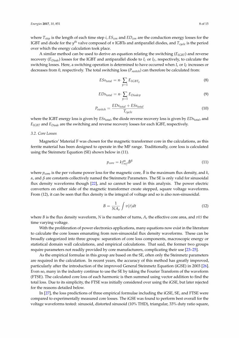
A detailed description of the iGSE is given in [26], and only a brief overview of its implementationis given here. The flux density waveform is first split into nc individual cycles, and then further intoits rising and falling sections; i.e., the cycle’s global minimum to maximum and global maximumto minimum, respectively. If there are multiple global maxima or minima, either can be chosen. Anexample flux density waveform is shown in Figure 7. It has been split into its rising and falling sections,with the minor loops in each identified in red; the black line forms the major loop of the rising andfalling sections.Energies 2017, 10, 851 9 of 15

Figure 7. Splitting of an example flux density waveform into its major and minor loops.

An algorithm, loosely based on rain flow analysis, was used here to identify and separate each minor loop from the major loops. Taking the rising section as an example, the algorithm adds each point in turn to a first set, s1, until a negative gradient is detected, i.e., point J in Figure 7. A new set is then created (s1+1), and each point is added to this until either the next negative gradient is reached (J’), after which an additional set is created or the end of the section is reached. Each set is then examined, starting at the final set sq. Any points greater than the set’s initial flux density, i.e., point J’ for the last set in this example or point J for the second set, are moved to the lower set, i.e., sq−1, until the first set s1 is reached. Now s1 contains a monotonically increasing major loop with sets s1+1 to sq holding each minor loop. The power loss can then be calculated separately for each loop and cycle using (13) and (14). = (2 ) ∙ 2 | | (13)

= 1 (∆ ) (14)

or, as a discrete function: = ∆ (15)

The total core loss is then determined by a weighted average of the power from each loop, as in (16), and the average loss of all of the cycles of the waveform calculated by applying (17). = (16)

= 1 (17)

where po is the core loss for each major or sub loop of the lth cycle, δBi and δti are the change in flux and time between time step i and i−1, and Tcycle and To are the periods of the cycle of the oth loop.

Using the core loss vs. flux density and frequency data from the core manufacturer’s data sheet, the Steinmetz parameters can be calculated from the three dimensional linear regression the logarithm of (11), shown in (18) ln( ) = + ln + ln (18)

Figure 7. Splitting of an example flux density waveform into its major and minor loops.

An algorithm, loosely based on rain flow analysis, was used here to identify and separate eachminor loop from the major loops. Taking the rising section as an example, the algorithm adds eachpoint in turn to a first set, s1, until a negative gradient is detected, i.e., point J in Figure 7. A new set isthen created (s1+1), and each point is added to this until either the next negative gradient is reached (J’),after which an additional set is created or the end of the section is reached. Each set is then examined,starting at the final set sq. Any points greater than the set’s initial flux density, i.e., point J’ for the lastset in this example or point J for the second set, are moved to the lower set, i.e., sq−1, until the firstset s1 is reached. Now s1 contains a monotonically increasing major loop with sets s1+1 to sq holdingeach minor loop. The power loss can then be calculated separately for each loop and cycle using (13)and (14).

kiGSE =k

(2π)α−1·2β−α∫ 2π

0 |cosθ|αdθ(13)

po =1To

∫ To

0kiGSE

∣∣∣∣dBdt

∣∣∣∣α(∆B)β−αdt (14)

or, as a discrete function:

po =kiGSE∆Bα−1

To∑i=1

∣∣∣∣ δBiδti

∣∣∣∣αδti (15)

The total core loss is then determined by a weighted average of the power from each loop,as in (16), and the average loss of all of the cycles of the waveform calculated by applying (17).

pcorel = ∑o=1

poTo

Tcycle(16)

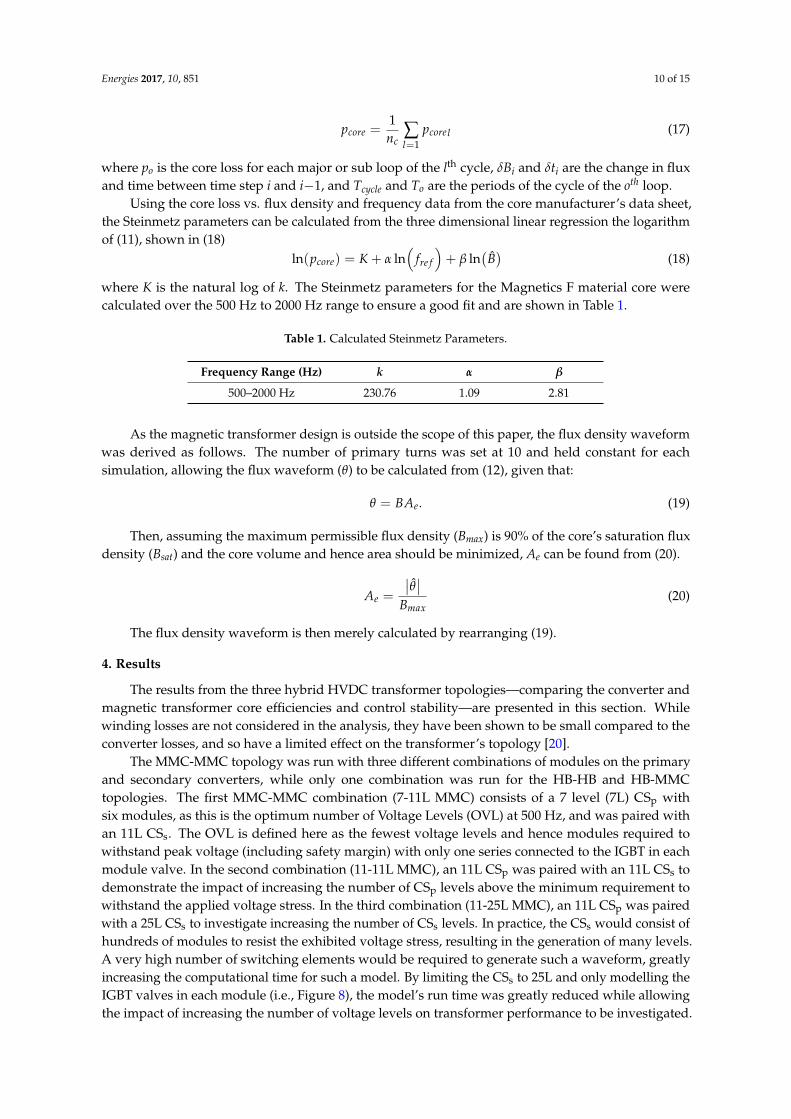
Energies 2017, 10, 851 10 of 15

pcore =1nc

∑l=1

pcorel (17)

where po is the core loss for each major or sub loop of the lth cycle, δBi and δti are the change in fluxand time between time step i and i−1, and Tcycle and To are the periods of the cycle of the oth loop.

Using the core loss vs. flux density and frequency data from the core manufacturer’s data sheet,the Steinmetz parameters can be calculated from the three dimensional linear regression the logarithmof (11), shown in (18)

ln(pcore) = K + α ln(

fre f

)+ β ln

(B̂)

(18)

where K is the natural log of k. The Steinmetz parameters for the Magnetics F material core werecalculated over the 500 Hz to 2000 Hz range to ensure a good fit and are shown in Table 1.

Table 1. Calculated Steinmetz Parameters.

Frequency Range (Hz) k α β

500–2000 Hz 230.76 1.09 2.81

As the magnetic transformer design is outside the scope of this paper, the flux density waveformwas derived as follows. The number of primary turns was set at 10 and held constant for eachsimulation, allowing the flux waveform (θ) to be calculated from (12), given that:

θ = BAe. (19)

Then, assuming the maximum permissible flux density (Bmax) is 90% of the core’s saturation fluxdensity (Bsat) and the core volume and hence area should be minimized, Ae can be found from (20).

Ae =

∣∣θ̂∣∣Bmax

(20)

The flux density waveform is then merely calculated by rearranging (19).

4. Results

The results from the three hybrid HVDC transformer topologies—comparing the converter andmagnetic transformer core efficiencies and control stability—are presented in this section. Whilewinding losses are not considered in the analysis, they have been shown to be small compared to theconverter losses, and so have a limited effect on the transformer’s topology [20].

The MMC-MMC topology was run with three different combinations of modules on the primaryand secondary converters, while only one combination was run for the HB-HB and HB-MMCtopologies. The first MMC-MMC combination (7-11L MMC) consists of a 7 level (7L) CSp withsix modules, as this is the optimum number of Voltage Levels (OVL) at 500 Hz, and was paired withan 11L CSs. The OVL is defined here as the fewest voltage levels and hence modules required towithstand peak voltage (including safety margin) with only one series connected to the IGBT in eachmodule valve. In the second combination (11-11L MMC), an 11L CSp was paired with an 11L CSs todemonstrate the impact of increasing the number of CSp levels above the minimum requirement towithstand the applied voltage stress. In the third combination (11-25L MMC), an 11L CSp was pairedwith a 25L CSs to investigate increasing the number of CSs levels. In practice, the CSs would consist ofhundreds of modules to resist the exhibited voltage stress, resulting in the generation of many levels.A very high number of switching elements would be required to generate such a waveform, greatlyincreasing the computational time for such a model. By limiting the CSs to 25L and only modelling theIGBT valves in each module (i.e., Figure 8), the model’s run time was greatly reduced while allowingthe impact of increasing the number of voltage levels on transformer performance to be investigated.

Energies 2017, 10, 851 11 of 15

It should be noted that the number of switches within the valves were varied to resist the differentvoltage and current stresses of each configuration. This did not impact on simulation time, as only thevalves were simulated as the number of switches was only taken into account for the loss calculations.Energies 2017, 10, 851 11 of 15

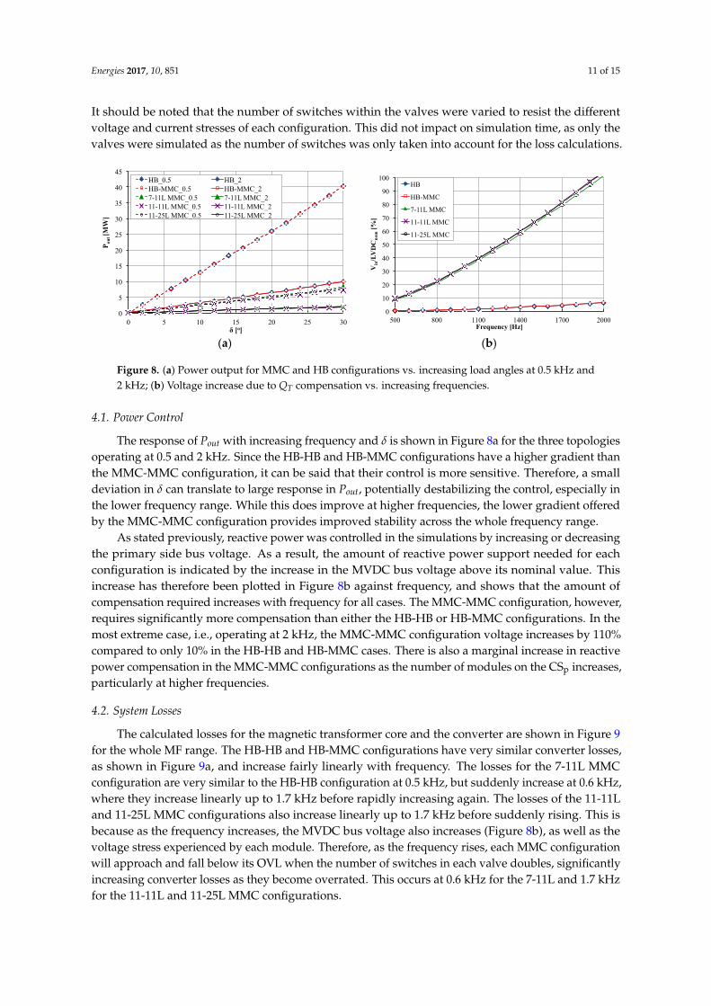
(a) (b)

Figure 8. (a) Power output for MMC and HB configurations vs. increasing load angles at 0.5 kHz and 2 kHz; (b) Voltage increase due to QT compensation vs. increasing frequencies.

As stated previously, reactive power was controlled in the simulations by increasing or decreasing the primary side bus voltage. As a result, the amount of reactive power support needed for each configuration is indicated by the increase in the MVDC bus voltage above its nominal value. This increase has therefore been plotted in Figure 8b against frequency, and shows that the amount of compensation required increases with frequency for all cases. The MMC-MMC configuration, however, requires significantly more compensation than either the HB-HB or HB-MMC configurations. In the most extreme case, i.e., operating at 2 kHz, the MMC-MMC configuration voltage increases by 110% compared to only 10% in the HB-HB and HB-MMC cases. There is also a marginal increase in reactive power compensation in the MMC-MMC configurations as the number of modules on the CSp increases, particularly at higher frequencies.

4.2. System Losses

The calculated losses for the magnetic transformer core and the converter are shown in Figure 9 for the whole MF range. The HB-HB and HB-MMC configurations have very similar converter losses, as shown in Figure 9a, and increase fairly linearly with frequency. The losses for the 7-11L MMC configuration are very similar to the HB-HB configuration at 0.5 kHz, but suddenly increase at 0.6 kHz, where they increase linearly up to 1.7 kHz before rapidly increasing again. The losses of the 11-11L and 11-25L MMC configurations also increase linearly up to 1.7 kHz before suddenly rising. This is because as the frequency increases, the MVDC bus voltage also increases (Figure 8b), as well as the voltage stress experienced by each module. Therefore, as the frequency rises, each MMC configuration will approach and fall below its OVL when the number of switches in each valve doubles, significantly increasing converter losses as they become overrated. This occurs at 0.6 kHz for the 7-11L and 1.7 kHz for the 11-11L and 11-25L MMC configurations.

0

5

10

15

20

25

30

35

40

45

0 5 10 15 20 25 30

P out

[MW

]

δ [o]

HB_0.5 HB_2 HB-MMC_0.5 HB-MMC_2 7-11L MMC_0.5 7-11L MMC_2 11-11L MMC_0.5 11-11L MMC_2 11-25L MMC_0.5 11-25L MMC_2

0

10

20

30

40

50

60

70

80

90

100

500 800 1100 1400 1700 2000

Vin

/LV

DC

nom

[%]

Frequency [Hz]

HB

HB-MMC

7-11L MMC

11-11L MMC

11-25L MMC

0

10

20

30

40

50

60

70

80

90

100

500 800 1100 1400 1700 2000

P cor

e [kW

/m3 ]

Frequency [Hz]

HB

HB-MMC

7-11L MMC

11-11L MMC

11-25L MMC

0

0.5

1

1.5

2

2.5

3

3.5

4

4.5

500 800 1100 1400 1700 2000

P los

s [%

]

Frequency [Hz]

HB

HB-MMC

7-11L MMC

11-11L MMC

11-25L MMC

OVL

(a) (b)

Figure 8. (a) Power output for MMC and HB configurations vs. increasing load angles at 0.5 kHz and2 kHz; (b) Voltage increase due to QT compensation vs. increasing frequencies.

4.1. Power Control

The response of Pout with increasing frequency and δ is shown in Figure 8a for the three topologiesoperating at 0.5 and 2 kHz. Since the HB-HB and HB-MMC configurations have a higher gradient thanthe MMC-MMC configuration, it can be said that their control is more sensitive. Therefore, a smalldeviation in δ can translate to large response in Pout, potentially destabilizing the control, especially inthe lower frequency range. While this does improve at higher frequencies, the lower gradient offeredby the MMC-MMC configuration provides improved stability across the whole frequency range.

As stated previously, reactive power was controlled in the simulations by increasing or decreasingthe primary side bus voltage. As a result, the amount of reactive power support needed for eachconfiguration is indicated by the increase in the MVDC bus voltage above its nominal value. Thisincrease has therefore been plotted in Figure 8b against frequency, and shows that the amount ofcompensation required increases with frequency for all cases. The MMC-MMC configuration, however,requires significantly more compensation than either the HB-HB or HB-MMC configurations. In themost extreme case, i.e., operating at 2 kHz, the MMC-MMC configuration voltage increases by 110%compared to only 10% in the HB-HB and HB-MMC cases. There is also a marginal increase in reactivepower compensation in the MMC-MMC configurations as the number of modules on the CSp increases,particularly at higher frequencies.

4.2. System Losses

The calculated losses for the magnetic transformer core and the converter are shown in Figure 9for the whole MF range. The HB-HB and HB-MMC configurations have very similar converter losses,as shown in Figure 9a, and increase fairly linearly with frequency. The losses for the 7-11L MMCconfiguration are very similar to the HB-HB configuration at 0.5 kHz, but suddenly increase at 0.6 kHz,where they increase linearly up to 1.7 kHz before rapidly increasing again. The losses of the 11-11Land 11-25L MMC configurations also increase linearly up to 1.7 kHz before suddenly rising. This isbecause as the frequency increases, the MVDC bus voltage also increases (Figure 8b), as well as thevoltage stress experienced by each module. Therefore, as the frequency rises, each MMC configurationwill approach and fall below its OVL when the number of switches in each valve doubles, significantlyincreasing converter losses as they become overrated. This occurs at 0.6 kHz for the 7-11L and 1.7 kHzfor the 11-11L and 11-25L MMC configurations.

Energies 2017, 10, 851 12 of 15

Energies 2017, 10, 851 11 of 15

(a) (b)

Figure 8. (a) Power output for MMC and HB configurations vs. increasing load angles at 0.5 kHz and 2 kHz; (b) Voltage increase due to QT compensation vs. increasing frequencies.

As stated previously, reactive power was controlled in the simulations by increasing or decreasing the primary side bus voltage. As a result, the amount of reactive power support needed for each configuration is indicated by the increase in the MVDC bus voltage above its nominal value. This increase has therefore been plotted in Figure 8b against frequency, and shows that the amount of compensation required increases with frequency for all cases. The MMC-MMC configuration, however, requires significantly more compensation than either the HB-HB or HB-MMC configurations. In the most extreme case, i.e., operating at 2 kHz, the MMC-MMC configuration voltage increases by 110% compared to only 10% in the HB-HB and HB-MMC cases. There is also a marginal increase in reactive power compensation in the MMC-MMC configurations as the number of modules on the CSp increases, particularly at higher frequencies.

4.2. System Losses

The calculated losses for the magnetic transformer core and the converter are shown in Figure 9 for the whole MF range. The HB-HB and HB-MMC configurations have very similar converter losses, as shown in Figure 9a, and increase fairly linearly with frequency. The losses for the 7-11L MMC configuration are very similar to the HB-HB configuration at 0.5 kHz, but suddenly increase at 0.6 kHz, where they increase linearly up to 1.7 kHz before rapidly increasing again. The losses of the 11-11L and 11-25L MMC configurations also increase linearly up to 1.7 kHz before suddenly rising. This is because as the frequency increases, the MVDC bus voltage also increases (Figure 8b), as well as the voltage stress experienced by each module. Therefore, as the frequency rises, each MMC configuration will approach and fall below its OVL when the number of switches in each valve doubles, significantly increasing converter losses as they become overrated. This occurs at 0.6 kHz for the 7-11L and 1.7 kHz for the 11-11L and 11-25L MMC configurations.

0

5

10

15

20

25

30

35

40

45

0 5 10 15 20 25 30

P out

[MW

]

δ [o]

HB_0.5 HB_2 HB-MMC_0.5 HB-MMC_2 7-11L MMC_0.5 7-11L MMC_2 11-11L MMC_0.5 11-11L MMC_2 11-25L MMC_0.5 11-25L MMC_2

0

10

20

30

40

50

60

70

80

90

100

500 800 1100 1400 1700 2000

Vin

/LV

DC

nom

[%]

Frequency [Hz]

HB

HB-MMC

7-11L MMC

11-11L MMC

11-25L MMC

0

10

20

30

40

50

60

70

80

90

100

500 800 1100 1400 1700 2000

P cor

e [kW

/m3 ]

Frequency [Hz]

HB

HB-MMC

7-11L MMC

11-11L MMC

11-25L MMC

0

0.5

1

1.5

2

2.5

3

3.5

4

4.5

500 800 1100 1400 1700 2000

P los

s [%

]

Frequency [Hz]

HB

HB-MMC

7-11L MMC

11-11L MMC

11-25L MMC

OVL

(a) (b)

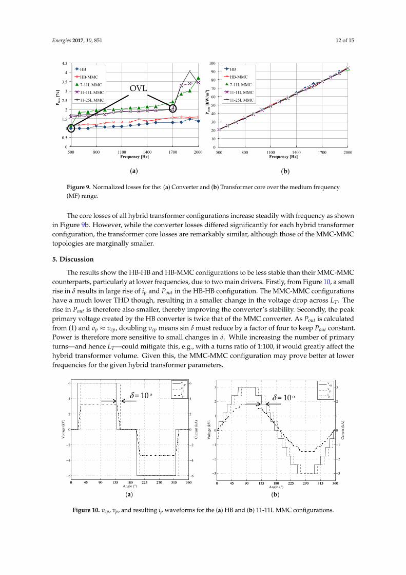
Figure 9. Normalized losses for the: (a) Converter and (b) Transformer core over the medium frequency(MF) range.

The core losses of all hybrid transformer configurations increase steadily with frequency as shownin Figure 9b. However, while the converter losses differed significantly for each hybrid transformerconfiguration, the transformer core losses are remarkably similar, although those of the MMC-MMCtopologies are marginally smaller.

5. Discussion

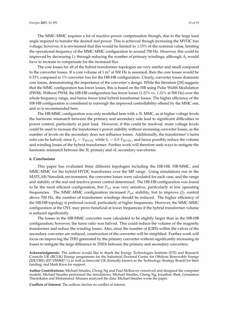
The results show the HB-HB and HB-MMC configurations to be less stable than their MMC-MMCcounterparts, particularly at lower frequencies, due to two main drivers. Firstly, from Figure 10, a smallrise in δ results in large rise of ip and Pout in the HB-HB configuration. The MMC-MMC configurationshave a much lower THD though, resulting in a smaller change in the voltage drop across LT. Therise in Pout is therefore also smaller, thereby improving the converter’s stability. Secondly, the peakprimary voltage created by the HB converter is twice that of the MMC converter. As Pout is calculatedfrom (1) and vp ≈ vcp, doubling vcp means sin δ must reduce by a factor of four to keep Pout constant.Power is therefore more sensitive to small changes in δ. While increasing the number of primaryturns—and hence LT—could mitigate this, e.g., with a turns ratio of 1:100, it would greatly affect thehybrid transformer volume. Given this, the MMC-MMC configuration may prove better at lowerfrequencies for the given hybrid transformer parameters.

Energies 2017, 10, 851 12 of 15

Figure 9. Normalized losses for the: (a) Converter and (b) Transformer core over the medium frequency (MF) range.

The core losses of all hybrid transformer configurations increase steadily with frequency as shown in Figure 9b. However, while the converter losses differed significantly for each hybrid transformer configuration, the transformer core losses are remarkably similar, although those of the MMC-MMC topologies are marginally smaller.

5. Discussion

The results show the HB-HB and HB-MMC configurations to be less stable than their MMC-MMC counterparts, particularly at lower frequencies, due to two main drivers. Firstly, from Figure 10, a small rise in δ results in large rise of ip and Pout in the HB-HB configuration. The MMC-MMC configurations have a much lower THD though, resulting in a smaller change in the voltage drop across LT. The rise in Pout is therefore also smaller, thereby improving the converter’s stability. Secondly, the peak primary voltage created by the HB converter is twice that of the MMC converter. As Pout is calculated from (1) and vp ≈ vcp, doubling vcp means sin δ must reduce by a factor of four to keep Pout constant. Power is therefore more sensitive to small changes in δ. While increasing the number of primary turns—and hence LT—could mitigate this, e.g., with a turns ratio of 1:100, it would greatly affect the hybrid transformer volume. Given this, the MMC-MMC configuration may prove better at lower frequencies for the given hybrid transformer parameters.

The MMC-MMC requires a lot of reactive power compensation though, due to the large load angle required to transfer the desired real power. This is achieved though increasing the MVDC bus voltage; however, it is envisioned that this would be limited to ±15% of the nominal value, limiting the operational frequency of the MMC-MMC configuration to around 700 Hz. However, this could be improved by decreasing LT through reducing the number of primary windings, although Ae would have to increase to compensate for the increased flux.

The core losses for all of the hybrid transformer topologies are very similar and small compared to the converter losses. If a core volume of 1 m3 at 500 Hz is assumed, then the core losses would be 0.33% compared to 1% converter loss for the HB-HB configuration. Clearly, converter losses dominate core losses, demonstrating the importance of the converter’s design. While the literature [28] suggests that the MMC configuration has lower losses, this is based on the HB using Pulse Width Modulation (PWM). Without PWM, the HB-HB configuration has fewer losses (1.21% vs. 1.31% at 500 Hz) over the whole frequency range, and hence lower total hybrid transformer losses. The higher efficiency of the HB-HB configuration is considered to outweigh the improved controllability offered by the MMC one, and so is recommended here.

Figure 10. vcp, vp, and resulting ip waveforms for the (a) HB and (b) 11-11L MMC configurations.

(a) (b)

δ = 10 o δ = 10 o

Figure 10. vcp, vp, and resulting ip waveforms for the (a) HB and (b) 11-11L MMC configurations.

Energies 2017, 10, 851 13 of 15

The MMC-MMC requires a lot of reactive power compensation though, due to the large loadangle required to transfer the desired real power. This is achieved though increasing the MVDC busvoltage; however, it is envisioned that this would be limited to ±15% of the nominal value, limitingthe operational frequency of the MMC-MMC configuration to around 700 Hz. However, this could beimproved by decreasing LT through reducing the number of primary windings, although Ae wouldhave to increase to compensate for the increased flux.

The core losses for all of the hybrid transformer topologies are very similar and small comparedto the converter losses. If a core volume of 1 m3 at 500 Hz is assumed, then the core losses would be0.33% compared to 1% converter loss for the HB-HB configuration. Clearly, converter losses dominatecore losses, demonstrating the importance of the converter’s design. While the literature [28] suggeststhat the MMC configuration has lower losses, this is based on the HB using Pulse Width Modulation(PWM). Without PWM, the HB-HB configuration has fewer losses (1.21% vs. 1.31% at 500 Hz) over thewhole frequency range, and hence lower total hybrid transformer losses. The higher efficiency of theHB-HB configuration is considered to outweigh the improved controllability offered by the MMC one,and so is recommended here.

The HB-MMC configuration was only modelled here with a 3L MMC, as at higher voltage levelsthe harmonic mismatch between the primary and secondary side lead to significant difficulties inpower control, particularly at part load. However, if this could be resolved, more voltage levelscould be used to increase the transformer’s power stability without increasing converter losses, as thenumber of levels on the secondary does not influence losses. Additionally, the transformer’s turnsratio can be halved, since v̂p = VMVDC while v̂s = 0.5·VHVDC, and hence possibly reduce the volumeand winding losses of the hybrid transformer. Further work will therefore seek ways to mitigate theharmonic mismatch between the 3L primary and nL secondary waveforms.

6. Conclusions

This paper has evaluated three different topologies including the HB-HB, HB-MMC, andMMC-MMC for the hybrid HVDC transformer over the MF range. Using simulations run in theMATLAB/Simulink environment, the converter losses were calculated for each case, and the rangeand stability of the real and reactive power control determined. The HB-HB configuration was foundto be the most efficient configuration, but Pout was very sensitive, particularly at low operatingfrequencies. The MMC-MMC configuration increased Pout stability, but to improve QT controlabove 700 Hz, the number of transformer windings should be reduced. The higher efficiency ofthe HB-HB topology is preferred overall, particularly at higher frequencies. However, the MMC-MMCconfiguration at the OVL may prove beneficial at lower frequencies if the hybrid transformer volumeis reduced significantly.

The losses in the HB-MMC converter were calculated to be slightly larger than in the HB-HBconfiguration; however, the turns ratio was halved. This could reduce the volume of the magnetictransformer and reduce the winding losses. Also, since the number of IGBTs within the valves of thesecondary converter are reduced, construction of the converter will be simplified. Further work willfocus on improving the THD generated by the primary converter without significantly increasing itslosses to mitigate the large difference in THDs between the primary and secondary converters.

Acknowledgments: The authors would like to thank the Energy Technologies Institute (ETI) and ResearchCouncils UK (RCUK) Energy programme for the Industrial Doctoral Center for Offshore Renewable Energy(IDCORE) (EP/J500847/1) as well as Innovate UK (formally known as the Technology Strategy Board) for theirfunding, and Mark Knos for support.

Author Contributions: Michael Smailes, Chong Ng and Paul McKeever conceived and designed the computermodels; Michael Smailes performed the simulations; Michael Smailes, Chong Ng, Jonathan Shek, GerasimosTheotokatos and Mohammad Abusara analyzed the data; Michael Smailes wrote the paper.

Conflicts of Interest: The authors declare no conflict of interest.

Energies 2017, 10, 851 14 of 15

References

1. Van Eeckhout, B.; Van Hertem, D.; Reza, M.; Srivastava, K.; Belmans, R. Economic comparison of VSC HVDCand HVAC as transmission system for a 300 MW offshore wind farm. Eur. Trans. Electr. Power 2010, 20,661–671. [CrossRef]

2. Arapogianni, A.; Moccia, J.; Wilkes, J. The European Offshore Wind Industry—Key Treds and Statistics 2012;European Wind Energy Association: Brussels, Belgium, 2013.

3. Northland Power Acquires Majority Equity Stake in North Sea Offshore Wind Farms From RWE Innogy.Available online: http://www.northlandpower.ca/Investor-Centre/News--Events/Recent_Press_Releases.aspx?MwID=1873377 (accessed on 2 February 2015).

4. Giller, P. Multi-Contracting for the First Project Financing in the German Offshore Wind Market: Projekt OffshoreWind Farm Meerwind Sud/Ost [288 MW Offshore Wind Farm]; WindMW GmbH: Bremerhaven, Germany, 2012.

5. Pulzer, M. Innovation for Offshore Substations. Real Power 2014, 35, 18–22.6. Ng, C.; McKeever, P. Next generation HVDC network for offshore renewable energy industry. In Proceedings

of the 10th IET International Conference on AC and DC Power Transmission (ACDC 2012), Birmingham, UK,4–5 December 2012; pp. 1–7.

7. Smailes, M.; Ng, C.; Shek, J.; Abusara, M.; Theotokatos, G.; McKeever, P. Hybrid, multi-megawatt HVDCtransformer for future offshore wind farms. In Proceedings of the 3rd Renewable Power GenerationConference RPG 2014, Naples, Italy, 24–25 September 2014; pp. 1–6.

8. Jovcic, D. Bidirectional, High-Power DC Transformer. IEEE Trans. Power Deliv. 2009, 24, 2276–2283.[CrossRef]

9. Denniston, N.; Massoud, A.M.; Ahmed, S.; Enjeti, P.N. Multiple-Module High-Gain High-Voltage DC-DCTransformers for Offshore Wind Energy Systems. IEEE Trans. Ind. Electron. 2011, 58, 1877–1886. [CrossRef]

10. Li, H.; Bai, X.; Wu, J. Study on modeling of high frequency power pulse transformer. In Proceedings of theWorld Automation Congress 2008 (WAC 2008), Hawaii, HI, USA, 28 September–2 October 2008; pp. 1–5.

11. Ortiz, G.; Biela, J.; Bortis, D.; Kolar, J.W. 1 Megawatt, 20 kHz, isolated, bidirectional 12 kV to 1.2 kV DC-DCconverter for renewable energy applications. In Proceedings of the 2010 International Power ElectronicsConference (IPEC), Sapporo, Japan, 21–24 June 2010; pp. 3212–3219.

12. Zhou, Y.; Macpherson, D.E.; Blewitt, W.; Jovcic, D. Comparison of DC-DC converter topologies for offshorewind-farm application. In Proceedings of the 6th IET International Conference on Power Electronics,Machines and Drives PEMD 2012, Bristol, UK, 27–29 March 2012; pp. 1–6.

13. De Doncker, R.W.; Divan, D.M.; Kheraluwala, M.H. A three-phase soft-switched high-power-density DC/DCconverter for high-power applications. IEEE Trans. Ind. Appl. 1991, 27, 63–73. [CrossRef]

14. Meier, S.; Kjellqvist, T.; Norrga, S.; Nee, H.-P. Design considerations for medium-frequency powertransformers in offshore wind farms. In Proceedings of the 13th European Conference on Power Electronicsand Applications, Barcelona, Spain, 8–10 September 2009; pp. 1–12.

15. Ortiz, G.; Biela, J.; Kolar, J.W. Optimized design of medium frequency transformers with high isolationrequirements. In Proceedings of the IECON 2010—36th Annual Conference on IEEE Industrial ElectronicsSociety, Glendale, AZ, USA, 7–10 November 2010; pp. 631–638.

16. Flourentzou, N.; Agelidis, V.G.; Demetriades, G.D. VSC-Based HVDC Power Transmission Systems:An Overview. IEEE Trans. Power Electron. 2009, 24, 592–602. [CrossRef]

17. Zhong, Y.; Finney, S.; Holliday, D. An investigation of high efficiency DC-AC converters for LVDC distributionnetworks. In Proceedings of the 7th IET International Conference on Power Electronics, Machines and Drives(PEMD 2014), Manchester, UK, 8–10 April 2014; pp. 1–6.

18. Marquardt, R. Modular Multilevel Converter: An universal concept for HVDC-Networks and extendedDC-Bus-applications. In Proceedings of the 2010 International Power Electronics Conference (IPEC),Sapporo, Japan, 21–24 June 2010; pp. 502–507.

19. Luth, T.; Merlin, M.M.C.; Green, T.C.; Hassan, F.; Barker, C.D. High-Frequency Operation of a DC/AC/DCSystem for HVDC Applications. IEEE Trans. Power Electron. 2014, 29, 4107–4115. [CrossRef]

20. Smailes, M.; Ng, C.; McKeever, P.; Fox, R.; Knos, M.; Shek, J. A modular, multi-megawatt, hybrid HVDCtransformer for offshore wind power collection and distribution. In Proceedings of the EWEA OffshoreWind Energy Conference, Paris, France, 17–20 November 2015.

Energies 2017, 10, 851 15 of 15

21. Rohner, S.; Bernet, S.; Hiller, M.; Sommer, R. Modulation, Losses, and Semiconductor Requirements ofModular Multilevel Converters. IEEE Trans. Ind. Electron. 2010, 57, 2633–2642. [CrossRef]

22. Mühlethaler, J.; Biela, J.; Kolar, J.W.; Ecklebe, A. Improved core-loss calculation for magnetic componentsemployed in power electronic systems. IEEE Trans. Power Electron. 2012, 27, 964–973. [CrossRef]

23. Bertotti, G. General properties of power losses in soft ferromagnetic materials. IEEE Trans. Magn. 1988, 24,621–630. [CrossRef]

24. Hargreaves, P.A.; Mecrow, B.C.; Hall, R. Calculation of iron loss in electrical generators using finite elementanalysis. In Proceedings of the 2011 IEEE International Electric Machines & Drives Conference IEMDC,Niagara Falls, ON, Canada, 15–18 May 2011; pp. 1368–1373.

25. Villar, I.; Viscarret, U.; Etxeberria-Otadui, I.; Rufer, A. Global Loss Evaluation Methods for NonsinusoidallyFed Medium-Frequency Power Transformers. IEEE Trans. Ind. Electron. 2009, 56, 4132–4140. [CrossRef]

26. Venkatachalam, K.; Sullivan, C.R.; Abdallah, T.; Tacca, H. Accurate prediction of ferrite core loss withnonsinusoidal waveforms using only Steinmetz parameters. In Proceedings of the 2002 IEEE Workshop onComputers in Power Electronics, Mayaguez, PR, USA, 3–4 June 2002; pp. 36–41.

27. Smailes, M.; Ng, C.; Fox, R.; Shek, J.; Abusara, M.; Theotokatos, G.; McKeever, P. Evaluation of coreloss calculation methods for highly non-sinusoidal inputs. In Proceedings of the 11th IET InternationalConference on AC and DC Power Transmission (ACDC), Birmingham, UK, 10–12 February 2015.

28. Tu, Q.; Xu, Z. Power losses evaluation for modular multilevel converter with junction temperaturefeedback. In Proceedings of the 2011 IEEE Power and Energy Society General Meeting, Detroit, MI, USA,24–29 July 2011; pp. 1–7.

© 2017 by the authors. Licensee MDPI, Basel, Switzerland. This article is an open accessarticle distributed under the terms and conditions of the Creative Commons Attribution(CC BY) license (http://creativecommons.org/licenses/by/4.0/).