A high-order method for weakly compressible flows

Klaus Kaiser*† and Jochen Schütz†

Institut für Geometrie und Praktische Mathematik Templergraben 55, 52062 Aachen, Germany

* IGPM, RWTH Aachen University, Templergraben 55, D-52062 Aachen† Faculty of Sciences, Hasselt University, Agoralaan Gebouw D, BE-3590 Diepenbeek

updated version of February 1, 2017

A U

G U

S T

2

0 1

6

P R

E P

R I N

T

4 5

6

A high-order method for weakly compressible flows

Klaus Kaiser∗,†, Jochen Schutz†

March 6, 2017

In this work, we introduce an IMEX discontinuous Galerkin solver for the weakly compressibleisentropic Euler equations. The splitting needed for the IMEX temporal integration is based onthe recently introduced reference solution splitting [1, 2], which makes use of the incompressiblesolution. We show that the overal method is asymptotic preserving.

*IGPM, RWTH Aachen University, Templergraben 55, 52062 Aachen

†Faculty of Sciences, Hasselt University, Agoralaan Gebouw D, BE-3590 Diepenbeek

1. Introduction

In this work, we consider the (weakly-)compressible isentropic Euler equations [3, 4] in dimensionless form,

ρt +∇ · (ρu) = 0

(ρu)t +∇ · (ρu⊗ u) +1

ε2∇p = 0.

(1)

The wave speeds in normal direction n of this (assumed two-dimensional) problem are

λ1 = u · n and λ2,3 = u · n± c

ε, (2)

which means that there is a convective and two acoustic waves. In what follows, we assume that the referenceMach number ε is small, i.e., ε 1, and all the other quantities are O(1), which physically means thatthe solution is a small disturbance of the incompressible solution. Indeed, it can be shown that undersuitable requirements on initial and boundary data (“well-preparedness”), there is convergence of densityand momentum (ρ, ρu) towards its incompressible counterpart as ε → 0, see [5, 6, 7] and the referencestherein. Furthermore, it is obvious that this problem constitutes a singularly perturbed equation in ε, as theequations change type in the limit.

Due to the change of type as ε→ 0, the equations get extremely stiff and therefore it is highly non-trivialto design efficient and stable algorithms. Explicit-in-time solving techniques have the drawback that theylead to a CFL condition in which the time step size ∆t must be proportional to ε∆x, where ∆x is a measurefor the spatial grid size. If it is not the goal to accurately resolve all the features, but only to resolve theconvective part of the flow, this condition is extremely restrictive, and a so called convective CFL condition

∆t .∆x

‖u‖ (3)

is preferable. Fully implicit-in-time methods, on the other hand, which are stable under such a CFLcondition, tend to add too much spurious diffusion [8].

1

In the past few years, so called IMEX (implicit-explicit) splitting schemes got more and more popularfor solving compressible flow problems, especially for low Mach numbers, see e.g. [9, 10, 11, 12, 13, 14,15, 16, 17, 18, 19] and the references therein. Optimally, such a scheme should be designed in a way thatslow waves are handled with an explicit (thus efficient) and fast waves are handled with an implicit (thusunconditionally stable) method. Of course such a strict splitting of waves is only possible in the linearone-dimensional case [20], and therefore, a suitable splitting for the nonlinear multidimensional case has tobe defined very carefully.

Over the past few years, many famous splittings for the Euler equations at low Mach number have beendesigned, beginning by the ground-breaking work of Klein [15]. For a non-exhaustive list, we refer to[10, 12, 14] and the references therein. However, many of those splittings have their shortcomings. It hasbeen reported [21] that Klein’s splitting seems to be unstable in some instances. (Which does not includeKlein’s original algorithm as it is based on a semi discrete decoupling of the pressure.) Furthermore, allof the mentioned splittings need a physical intuition and are not directly extendable to other singularlyperturbed differential equations.

To partly overcome these shortcomings, we have over the past few years developed a new type of splittingthat is based on the ε = 0 (“incompressible”) solution of the problem. The splitting, termed RS-IMEX(see Sec. 3), is generic in the sense that it can in principle be applied to any type of singularly perturbedequation, including singularly perturbed ODEs [1] and the isentropic Euler equations [2]. Related ideas havealready been published earlier, for the shallow water equations in [10, 22] and for kinetic equations in [23],a stability analysis of the splitting has been done in [21] and [24].

In [1], we have applied the splitting idea to singularly perturbed ordinary differential equations with high-order IMEX discretizations, namely IMEX linear multistep methods [25, 26, 27] and IMEX Runge-Kuttamethods [28, 29, 30, 31, 32, 33, 34]. In [2], we have applied the splitting idea to a low-order finite volumescheme for the isentropic Euler equations. In both publications, we have seen that the newly developedsplitting can be highly advantageous. This present work is a ’natural’ extension of those previous works: Wecombine a high-order-in-time IMEX Runge-Kutta scheme with a high-order-in-space discontinuous Galerkin(DG) method (see [35, 36, 37, 38, 39] for classical DG and [40, 41, 42] for IMEX DG) using the newlydeveloped splitting. The difficulty herein lies in the subtle interplay of the stiffness induced by the singularcharacter of the equation and the stiffness induced by the high-order approximation of both spatial andtemporal variables. We show how to choose the numerical viscosities in such a way that the resulting methodis asymptotically consistent, see e.g. [43], which means that its ε → 0 limit is a consistent discretizationof the corresponding incompressible equations. Numerical results show the convergence of the method. Itturns out that the overal scheme is indeed stable under a convective CFL condition (3), order degradationis not observed.

This paper is organized as follows: The governing equations are discussed in Sec. 2, the splitting andcorresponding IMEX time integration are presented in Sec. 3. The fully discrete method is introduced inSec. 4, with its asymptotic consistency property being discussed in Sec. 5. Numerical results are shown inSec. 6. As usual, the paper ultimately gives some conclusion and outlook in the last Sec. 7. To make thepaper more self-consistent, the Butcher tableaux for the used IMEX Runge-Kutta schemes are shown in theappendix in Sec. A.

2. Governing equations

Let Ω ⊂ R2 be a two-dimensional domain, and consider the isentropic Euler equations as in (1), with ρ ∈ Rdensity and u = (u, v)T ∈ R2 velocity in x− and y−direction, respectively. p denotes pressure given forpolytropic fluids as p(ρ) := κργ with a κ > 0 and a γ ≥ 1. Note that the (scaled) characteristic Mach

2

number ε is given by

ε :=u∗√

p(ρ∗)/ρ∗,

where u∗ and ρ∗ are the corresponding characteristic values for velocity and density, respectively, used tonondimensionalize the equation. The isentropic Euler equations can directly be rewritten as a conservationlaw in divergence form

wt +∇ · f(w) = 0, ∀x ∈ Ω, t ∈ (0, T ) (4)

w(x, t = 0) = w0(x), ∀x ∈ Ω (5)

with

w :=

(ρρu

)and f(w) :=

(ρu

ρu⊗ u+ 1ε2p · Id

),

where Id denotes the two dimensional identity matrix. w0 are given initial data. Computing the eigenvaluesof ∂wf(w) · n gives the characteristic wave speeds

λ1 = u · n and λ2,3 = u · n± c

ε, (2)

where c =√

γpρ denotes the speed of sound of the system. Obviously, these eigenvalues are on different

scales w.r.t. ε. Scales can be best understood by considering an asymptotic expansion of every quantity,namely

w = w(0) + εw(1) + ε2w(2) +O(ε3). (6)

Inserting this expansion into the isentropic Euler equations (1), collecting terms with equal power of ε andtaking the limit ε→ 0 leads to the incompressible Euler equations [5]

ρ(0) ≡ const > 0, ∇ · u(0) = 0,

(u(0))t +∇ · (u(0) ⊗ u(0)) +∇p(2)

ρ(0)= 0.

(7)

The existence of a limit necessitates the use of specially designed initial data, see e.g. [5, 6, 7] and thereferences therein, which we introduce in the sequel for the isentropic Euler equations:

Definition 1 (Well prepared initial conditions). We call initial data w0 = (ρ0, ρ0u0)T for the compressibleequation well prepared if they can be represented by an asymptotic expansion as in (6) and fulfill

ρ0 = const +O(ε2), ∇ · u0 = O(ε).

Well prepared initial data, together with sufficient smoothness, guarantee the convergence of the solution asε→ 0 [5].

3. RS-IMEX time integration

The core idea of IMEX schemes is to separate stiff and non-stiff parts, and then to treat the former onesimplicitly, and the latter ones explicitly. For the ease of presentation, we start by considering the simplestsetting of all IMEX frameworks, the IMEX-Euler semi discretization to define the splitting. Then, we extendthe proceeding to IMEX Runge-Kutta methods.

The temporal domain is given by [0, T ] with T ∈ R+. To define our methods, we have to split this domaininto N + 1 time instances tn := n∆t,

0 = t0 < . . . < tn < . . . < tN = T.

Uniform time slabs are not a necessity, but are used for notational convenience.

3

3.1. RS-IMEX splitting

We assume for the moment that a splitting of the convective flux into

f(w) = f(w) + f(w) (8)

is already given. Then, applied to (4), the time-discrete IMEX-Euler scheme is defined by

wn+1 −wn + ∆t∇ ·(f(wn+1) + f(wn)

)= 0. (9)

Note that f is the part that is treated implicitly, while f is the part that is treated explicitly. In thefollowing the upper index n of wn corresponds to the numerical solution - with respect to time - at timeinstance tn.

As already pointed out in the introduction, the choice of a splitting of the convective flux function f is acore ingredient to obtain a stable and efficient numerical method in the low-Mach range. This work relieson the recently introduced RS-IMEX splitting [1, 2, 21], where RS stands for reference solution and denotesthe limit-solution w(0) = (ρ(0), ρ(0)u(0))

T , see (7). The splitting relies on a linearization of the flux functionf around w(0) being used in the stiff part. For a more detailed derivation of the RS-IMEX splitting werefer to [1, 2], but also to [23, 10, 22] for earlier applications of a similar idea. More formally the RS-IMEXsplitting is given in the following definition.

Definition 2 (RS-IMEX). The RS-IMEX splitting is defined by

f(w) = f(w(0)) + ∂wf(w(0)) · (w −w(0)),

f(w) = f(w)− f(w),

where w(0) denotes the asymptotic solution solution w(0) = (ρ(0), ρ(0)u(0))T from (7), ∂wf denotes the

Jacobian of f .

Due to its definition, f is linear in w and, as this part is treated implicitly, the resulting system can besolved efficiently by a linear solution technique. Note that, although the idea stems from a linearization,there is no second-order linearization error of the flux, because remaining terms are collected in f . Applyingthe definition of f given in (4) to the RS-IMEX splitting, one can directly compute the flux functions f andf for the isentropic Euler equations:

Definition 3 (RS-IMEX splitting for the isentropic Euler equations). The RS-IMEX splitting for the is-tentropic Euler equations is given by

f(w) =

(ρu

−ρu(0) ⊗ u(0) + ρu⊗ u(0) + ρu(0) ⊗ u+ 1ε2

(p(ρ(0)) + p′(ρ(0))(ρ− ρ(0))

)· Id

),

f(w) =

(0

ρ(u− u(0))⊗ (u− u(0)) + 1ε2

(p(ρ)− p(ρ(0))− p′(ρ(0))(ρ− ρ(0))

)· Id

).

Remark 1. Note that the RS-IMEX splitting idea as given in Def. 2 can directly be extended to a widerange of different singularly perturbed equations.

Remark 2. In contrast to f , both f and f depend - through the use of the reference quantity w(0) -explicitly on t. We do not add t as an additional variable to the fluxes to keep the notation short. It willbecome important in the definition of the IMEX-Runge-Kutta scheme, because technically, we do not treatan autonomous differential equation any more.

That f is indeed ’non-stiff’ is indicated by the following lemma:

4

Lemma 1. 1. The eigenvalues of ∂wf(w) · n of are given by

λ =

0(u− u(0)) · n2(u− u(0)) · n

.

2. The in magnitude largest eigenvalues of the Jacobian of the implicit part are in O(

1ε

).

We can conclude two different things from La. 1. First, the stiffness of the equation is completely hiddenin the implicit part. Second, if we take the limit ε→ 0, the influence of the explicit part vanishes.

3.2. IMEX Runge-Kutta method

We have discussed the RS-IMEX splitting in the context of a straightforward IMEX-Euler discretization,see (9). The extension to higher-order methods is evident, methods of choice are, e.g., high-order IMEXRunge-Kutta methods [28, 29, 30, 31, 32, 33, 34] or high-order IMEX linear multistep methods [25, 26, 27].In this work, we consider IMEX Runge-Kutta methods, where we restrict ourselves to a (relatively large)subclass which we identified as important in our previous work [1]:

• We only consider IMEX Runge-Kutta methods which are globally stiffly accurate (GSA), see e.g. [29].In short this is fulfilled if the update step is equal to the last internal stage of the Runge-Kutta method.This corresponds to the first same as last property for an explicit and the stiffly accurate propertyfor an implicit Runge-Kutta method. The IMEX Runge-Kutta methods are fully defined by the twoButcher tableaux A and A and the corresponding temporal coefficients c and c.

• We only consider IMEX Runge-Kutta methods where the implicit matrix A is a lower triangular one,such that in every internal stage only one implicit variable occurs. This is mostly due to efficiencyreasons.

• We only consider IMEX Runge-Kutta methods of type A or type CK. This is given if the implicitmatrix A is invertible (type A) or the first entry of the implicit matrix equals 0 and the remainingsubmatrix is invertible (type CK). See Def. 4 for more details. For a more detailed classification ofIMEX Runge-Kutta methods we refer to [44].

In the following, we first introduce such a Runge-Kutta scheme for the semi-discrete-in-time discretizationof the Euler equations (4).

Definition 4 (GSA IMEX Runge-Kutta scheme for (4)). For every tn+1 = tn + ∆t do the following:

1. For i = 1, . . . , s solve

wn,i −wn + ∆t

i∑j=1

Ai,j∇ · f(wn,j) +

i−1∑j=1

Ai,j∇ · f(wn,j)

= 0, (10)

where wn,i denotes the solution of the ith internal stage. Note that f is evaluated at time tn,j, and fat tn,j, with

tn,j := tn + cj∆t, tn,j := tn + cj∆t,

see also Rem. 2.

2. Set wn+1 := wn,s.

5

The coefficients of the IMEX RK method are given by two Butcher tableaux, the one with overhats referringto the explicit, the other to the implicit part. Because of our restrictions on the Runge-Kutta method, theimplicit coefficient matrix has to fulfill Aii 6= 0 for i = 2 . . . s. For a type A method, there even holds A11 6= 0in addition.

Based on our work in [1], we use the IMEX Runge-Kutta methods presented in Tbl. 2, 3, 4 and 5; alsogiven in [28, 33, 34]. A classification of these methods can be seen in Tbl. 1.

4. IMEX DG method

High-order temporal integration has to be coupled to a high-order spatial discretization. The methodof choice of the latter in this work is a combination of a high-order IMEX Runge-Kutta method with ahigh-order discontinuous Galerkin (DG) discretization [35, 36, 37, 38, 39], yielding an IMEX DG method[40, 41, 42].

4.1. Preliminary definitions

We assume that the periodic domain Ω ⊂ R2 is divided into ne ∈ N non-overlapping cells Ωk as

ne⋃k=1

Ωk = Ω and Ωk ∩ Ωi = ∅ ∀k 6= i.

The boundary of the cell Ωk is denoted by ∂Ωk and nk denotes the corresponding outward normal vector.On this triangulation Ωk we define a broken polynomial space by

Vq := v ∈ L2(Ω) : v|Ωk∈ Pq(Ωk) ∀ k = 1, . . . ,ne,

where Pq(Ωk) denotes the space of all polynomial functions with maximum degree q on cell Ωk. For system-valued functions (there are three components in the Euler equations) we define the corresponding space

V 3q := Vq × Vq × Vq.

Of course an adaptive choice of q is possible. For a value x ∈ ∂Ωk, we define the interior (−) and exterior(+) value, respectively, of a function σ ∈ Vq by

σ∓(x) := lim0<δ→0

σ(x∓ δnk). (11)

If a boundary is considered independently of a specific cell, we can in a similar way define a value of σ∓

based on an arbitrary, but fixed direction of edge normal vectors.

4.2. IMEX Runge-Kutta Discontinuous Galerkin method

Following the common steps [39], we can define the DG residual of both ∇ · f(w) and ∇ · f(w) by thequantities

R(w∆x;ϕ) := −∫

Ωf(w∆x) · ∇ϕdx+

ne∑k=1

∫∂Ωk

h(w−∆x,w+∆x)ϕ · nkds, and

R(w∆x;ϕ) := −∫

Ωf(w∆x) · ∇ϕdx+

ne∑k=1

∫∂Ωk

h(w−∆x,w+∆x)ϕ · nkds,

6

respectively. Note that integration over Ω is to be understood in the cell-wise sense. h and h are stiff andnon-stiff numerical flux function, respectively, given by

h(w−,w+) :=1

2

(f(w−) + f(w+)

)+

1

2Diag

(1

ε2, 1, 1

)(w− −w+

)· n, (12)

h(w−,w+) :=1

2

(f(w−) + f(w+)

)+ ε

(w− −w+

)· n. (13)

Remark 3. The numerical flux is of Rusanov-type.

• Let us note that a somewhat similar choice of the stiff stabilization, for the equations in primitivevariables, has been made in [45], motivated by the fundamental work of Turkel [46], who introducedpreconditioning of the time derivative to enhance steady-state computations for low-Mach flows.

• The choice of the non-stiff stabilization is motivated by La. 1, as the eigenvalues of ∂wf(w) ·n are inO(ε) if one assumes that u = u(0) +O(ε).

• As observed in [10] and [2], the choice of the numerical flux function affects asymptotic consistency.The choice here guarantees the latter important property.

The extension of Def. 4 to the fully discrete DG scheme can be done in a straightforward way by replacingfluxes f by discrete fluxes R. To get the notation right, we shortly review this discretization here:

Definition 5 (High-order method for weakly compressible flows). For every tn+1 = tn+∆t do the following:

1. For i = 1, . . . , s solve∫Ω

(wn,i

∆x −wn∆x

)ϕdx+ ∆t

i∑j=1

Ai,jR(wn,j∆x;ϕ) +

i−1∑j=1

Ai,jR(wn,j∆x;ϕ)

= 0 ∀ϕ ∈ V 3q , (14)

where wn,i∆x denotes the solution of the ith internal stage. Also R and R depend on time t and are

evaluated at

tn,j := tn + cj∆t, and tn,j := tn + cj∆t,

respectively.

2. Set wn+1∆x := wn,s

∆x.

In Def. 5, we have summarized the final algorithm to be used in this work. With this, we are now readyto prove asymptotic consistency.

5. Asymptotic consistency

As mentioned in Sec. 1, our aim is to develop a method whose ε→ 0 limit is a consistent discretization ofthe limit equation (7), which means that it preserves the asymptotic behavior of the corresponding equation.We prove that our method is asymptotically consistent, for the ease of presentation in two steps:

1. First, we consider the semi discrete (discrete in time) setting (10).

2. Then, we consider the fully discrete setting (14).

Unfortunately, the methods we have introduced require a lot of notation. The following list gives anoverview of the terms we use.

7

Remark 4 (Notation). 1. An upper index n, e.g., un, indicates that the quantity is given at time levelt = tn.

2. An additional upper index i, e.g., un,i, denotes the ith internal stage of an IMEX Runge-Kutta method.

3. A lower index ∆x, e.g., u∆x, denotes a variable which belongs to a discontinuous Galerkin discretiza-tion.

4. An additional upper index − or +, e.g., u∓∆x, denotes the interior or exterior value corresponding toan edge, see (11).

5. A lower index in brackets (i), e.g., u(i), denotes a variable which belongs to the ith component of anasymptotic expansion, see (6)

5.1. Semi discrete setting

We start by considering the RS-IMEX splitting for the isentropic Euler equation (1) coupled to an IMEXRunge-Kutta temporal discretization as in (10).

Theorem 1. The RS-IMEX splitting, given in Def. 3, coupled to an IMEX Runge-Kutta temporal dis-cretization as given in Def. 4 is asymptotically consistent if well prepared initial data at time t = 0 andperiodic boundary conditions are used.

Proof. We first show that, given wn is well-prepared, also wn+1 is well-prepared. Because w0 is well-prepared, one can then inductively prove that all wn are well-prepared.

We assume that all the (discrete) quantities can be represented with an asymptotic expansion as in (6),e.g.,

(ρu)n,j = (ρu)n,j(0) + ε(ρu)n,j(1) + . . . .

If A1,1 = 0, which happens for type CK methods, then the first internal stage is equal to the previous timeinstance wn

∆x. It is therefore directly well prepared. Therefore, we consider the ith internal stage with

Aii 6= 0.Because the numerical density is constant up to O(ε2), we know that its zeroth-order expansion is equal

to the reference density ρ(0). Therefore, considering the O(ε−2) terms of the momentum equation, we obtain

0 =∇Ai,iε2

(p(ρ(0)) + p′(ρ(0))(ρ

n,i(0) − ρ(0))

)⇔ 0 =∇Ai,i

ε2

(p′(ρ(0))ρ

n,i(0)))

⇔ 0 =∇ρn,i(0).

Thus the limit density is constant in space. Next we consider the O(1) terms of the first equation andintegrate over the whole domain. Using the periodic boundary conditions we get∫

Ωρn,i(0) − ρ

n(0)dx = 0.

Since both values are constant in space, we can conclude that ρn,i(0) is constant in i, and therefore it is equal

to ρ(0). Considering again the O(1) terms of the mass equation we now obtain∑j

Aij∇ · (ρu)n,j(0) = 0.

8

Since wn is well-prepared, one can then inductively show that all stage values (ρu)n,i(0) are solenoidal, and one

can directly obtain ∇ · (ρu)n,i(0) = 0 if Aii 6= 0. This means that all stage values are well-prepared. Becausethe underlying IMEX RK method is globally stiffly accurate, the update step is equal to the last stage. Thisautomatically proves that the values wn+1 are well-prepared.

The proof is finalized by the remark that the discrete limit momentum equation is a consistent discretiza-tion of the limit momentum equation.

A question which arises from the use of the RS-IMEX splitting is how to compute the limit solution. Inan ideal case this solution is given, but generally we need a numerical method for its computation. It isuseful to compute the limit solution in such a way that it corresponds to the solution of the limit method.

Theorem 2. The limit of the semi discrete method (10) is a discretization that is fully implicit-in-time.

Proof. We consider the ith internal stage and add a zero as

ρ(0)un,j(0) ⊗ u

n,j(0) − ρ(0)u

n,j(0) ⊗ u

n,j(0) ,

then the limit numerical method reads (see also Def. 3)(0

ρ(0)un,i(0)

)=

(0

ρ(0)un(0)

)

−∆t∑j

Aij∇ ·(

un,j(0)

−ρ(0)(un,j(0) − u(0)(t

n,j))⊗ (un,j(0) − u(0)(tn,j)) + ρ(0)u

n,j(0) ⊗ u

n,j(0) + p′(ρ(0))ρ

n,j(2) · Id

)

−∆t∑j

Aij∇ ·(

0

ρ(0)(un,j(0) − u(0)(t

n,j))⊗ (un,j(0) − u(0)(tn,j)) +

(pn,j(2) − p′(ρ(0))ρ

n,j(2)

)· Id

).

We show that the limit method corresponds to a fully implicit method with the help of mathematicalinduction. Therefore we assume that the reference solution equals to the limit numerical solution for thei−1 previous stages (which should be given for the first instance due to the initial data). Additionally, fromthe asymptotic expansion one concludes

pn,i(2) = p′(ρ(0))ρn,i(2).

Finally, this all together simplifies to(0

ρ(0)un,i(0)

)=

(0

ρ(0)un(0)

)

+ ∆t∑j

Aij∇ ·(

un,i(0)

−ρ(0)(un,i(0) − u(0)(t

n,i))⊗ (un,i(0) − u(0)(tn,i)) + ρ(0)u

n,i(0) ⊗ u

n,i(0) + pn,i(2) · Id

),

which is a fully implicit discretization of the incompressible equation with additional terms in (un,i(0) −u(0)(t

n,i)). If u(0)(tn,i) has been computed by a fully implicit method (which takes only the implicit part

of the used IMEX Runge-Kutta method), the two solutions correspond to each other. This concludes theproof.

9

5.2. Fully discrete setting

Here, we consider the fully discrete setting, i.e., temporal discretization with an IMEX Runge-Kutta methodand spatial discretization with a DG method, see (14). To clarify the choice of the numerical diffusioncoefficients in (12), we start with the following lemma:

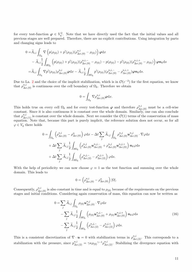
Lemma 2. Let the function σ∆x ∈ Vq be such that∫∂Ωk

(σ−dx − σ+∆x)ϕ−ds = 0, ∀ϕ ∈ Vq, ∀k = 1, . . . ,ne . (15)

Then, σ∆x is continuous.

Proof. We can choose ϕ = σ∆x in (15) and obtain∫∂Ωk

(σ−∆x − σ+∆x)σ−∆xds = 0

on every cell Ωk. Summing up over the whole domain and rearranging terms leads to

0 =∑k

∫∂Ωk

(σ−∆x − σ+∆x)σ−∆xds =

∑e

∫e(σ−∆x − σ+

∆x)2ds.

This means that σ−∆x = σ+∆x and therefore the quantity σ∆x is continuous over every cell boundary.

This lemma has a direct consequence for the numerical solution, namely, if we can show that the numericalstabilization of one quantity lives on a different scale (with respect to ε) than the rest of the correspondingequation, the ε = 0 limit of this quantity is continuous. We will apply this to the momentum equation andshow that the discrete approximation to ρ(0) is continuous, and one can then easily prove that it is constant.

Theorem 3. The RS-IMEX splitting, given in Def. 3, coupled to an IMEX Runge-Kutta temporal dis-cretization as given in Def. 5 is asymptotically consistent if periodic boundary conditions and discretely wellprepared initial data, see (16), at time t = 0 are used.

Proof. The proof is similar as before. We show inductively, starting from n = 0, that given well-preparedvalues wn

∆x, the algorithm preserves the well-preparedness. More precisely, we show that the internal stage

wn,i∆x of the RS-IMEX DG method fulfills ρn,i∆x = ρ(0) + O(ε2), and ∇ · u∆x,(0) = 0 in a discrete sense, see

(16) (i.e., it is well prepared in a discrete sense) if all the previous internal stages and the previous timeinstances are also discretely well prepared, and there holds that ρn∆x = ρ(0) + O(ε2). Together with thewell-preparedness at time t = 0 and the GSA property, this yields the well-preparedness of all discretequantities.

Note that if A1,1 = 0 then the first internal stage is equal to the previous time instance wn∆x, thus it

is directly well prepared. Therefore we now consider a given i such that Ai,i 6= 0. We assume that everyquantity can be expressed by an asymptotic expansion as in (6), e.g.,

ρn∆x = ρn∆x,(0) + ερn∆x,(1) + ε2ρn∆x,(2) +O(ε3).

Due to the numerical stabilization the only terms in O(ε−2) in the momentum equation are the pressureterms, thus

0 =Ai,i

∫Ωk

(p(ρ(0)) + p′(ρ(0))(ρ

n,i∆x,(0) − ρ(0))

)∇ϕdx

− Ai,i1

2

∫∂Ωk

(p(ρ(0)) + p′(ρ(0))(ρ

n,i,−∆x,(0) − ρ(0)) + p(ρ(0)) + p′(ρ(0))(ρ

n,i,+∆x,(0) − ρ(0))

)ϕnkdx

10

for every test-function ϕ ∈ V 2q . Note that we have directly used the fact that the initial values and all

previous stages are well prepared. Therefore, there are no explicit contributions. Using integration by partsand changing signs leads to

0 =Ai,i

∫Ωk

∇(p(ρ(0)) + p′(ρ(0))(ρ

n,i∆x,(0) − ρ(0))

)ϕdx

− Ai,i1

2

∫∂Ωk

(p(ρ(0)) + p′(ρ(0))(ρ

n,i,−∆x,(0) − ρ(0))− p(ρ(0))− p′(ρ(0))(ρ

n,i,+∆x,(0) − ρ(0))

)ϕnkds

=Ai,i

∫Ωk

∇p′(ρ(0))ρn,i∆x,(0)ϕdx− Ai,i

1

2

∫∂Ωk

p′(ρ(0))(ρn,i,−∆x,(0) − ρ

n,i,+∆x,(0))ϕnkds.

Due to La. 2 and the choice of the implicit stabilization, which is in O(ε−2) for the first equation, we knowthat ρn,i∆x,(0) is continuous over the cell boundary of Ωk. Therefore we obtain

0 =

∫Ωk

∇ρn,i∆x,(0)ϕdx.

This holds true on every cell Ωk and for every test-function ϕ and therefore ρn,i∆x,(0) must be a cell-wiseconstant. Since it is also continuous it is constant over the whole domain. Similarly, one can also concludethat ρn,i∆x,(1) is constant over the whole domain. Next we consider the O(1) terms of the conservation of massequation. Note that, because this part is purely implicit, the reference solution does not occur, so for allϕ ∈ Vq there holds

0 =

∫Ωk

(ρn,i∆x,(0) − ρ

n∆x,(0)

)ϕdx−∆t

∑j

Ai,j

∫Ωk

ρn,j∆x,(0)un,j∆x,(0) · ∇ϕdx

+ ∆t∑j

Ai,j1

2

∫∂Ωk

(ρn,j∆x,(0)u

n,j,−∆x,(0) + ρn,j∆x,(0)u

n,j,+∆x,(0)

)nkϕds

+ ∆t∑j

Ai,j1

2

∫∂Ωk

(ρn,j,−∆x,(2) − ρ

n,j,+∆x,(2)

)ϕds.

With the help of periodicity we can now choose ϕ ≡ 1 as the test function and summing over the wholedomain. This leads to

0 =(ρn,i∆x,(0) − ρ

n∆x,(0)

)|Ω|.

Consequently, ρn,i∆x,(0) is also constant in time and is equal to ρ(0) because of the requirements on the previousstages and initial conditions. Considering again conservation of mass, this equation can now be written as

0 =∑j

Ai,j

∫Ωk

ρ(0)un,j∆x,(0) · ∇ϕdx

−∑j

Ai,j1

2

∫∂Ωk

(ρ(0)u

n,j,−∆x,(0) + ρ(0)u

n,j,+∆x,(0)

)nkϕds (16)

−∑j

Ai,j1

2

∫∂Ωk

(ρn,j,−∆x,(2) − ρ

n,j,+∆x,(2)

)ϕds.

This is a consistent discretization of ∇ · u = 0 with stabilization terms in ρn,i∆x,(2). This corresponds to a

stabilization with the pressure, since pn,i∆x,(2) = γκρ(0)γ−1ρn,i∆x,(2). Stabilizing the divergence equation with

11

the pressure is also used in literature for discontinuous Galerkin methods for incompressible equations, seee.g. [47].

As for the semi discrete case, it is straightforward to see that the limit momentum equation is a consistentdiscretization of the corresponding equation. Thus the method is asymptotically consistent.

This section is finalized with some remarks:

Remark 5. • The choice of the numerical flux function is essential for the previous theorem. Takingimplicit stabilization coefficients in O(1), periodic boundary conditions and polynomial degree q = 0results in a method which is not guaranteed to be AC. In [2], this problem has been solved by using adifferent type of boundary condition, based on the work of [14]. In [48], this problem is solved by addingimplicit diffusion to the mass equation, which is similar to the choice of the numerical flux functionspresented in this work.

• The proof of the asymptotic consistency does not rely on the fact that the equations are two-dimensional.In fact, the three-dimensional case is also covered.

6. Numerical results

In this section we consider an example with exact solution to investigate the numerical method in terms ofstability and accuracy. The high-order vortex is given by a pressure function p(ρ) = 1

2ρ2 and periodic initial

conditions

ρ0(x, y) = 2 + 250, 000ε2

12e

2∆r ∆r − Ei

(2

∆r

)r < 1

2

0 otherwise

u0(x, y) =

(1/20

)+ 500

(12 − yx− 1

2

)·e

1∆r r < 1

2

0 otherwise,

where r :=√

(x− 12)2 + (y − 1

2)2 and ∆r := r2− 14 . The solution is a transport of the vortex in x-direction,

i.e.

ρ(x, y, t) = ρ0

(x− 1

2t, y

), u(x, y, t) = u0

(x− 1

2t, y

).

The high-order vortex can be seen as a high-order extension to a vortex defined by Bispen et al. [10]. Notethat the vortex is defined with the help of the exponential integral function

Ei(x) :=

∫ x

−∞

et

tdt.

This exponential integral function is, amongst others, implemented in the boost package [49, 50], which isused in this implementation. The finite element code is based on the software Netgen [51]; linear systemsare solved through PETSc [52, 53, 54].

Remark 6. In the following, if not stated otherwise, we use an ”exact” reference solution. This meansthat we project the exact reference solution onto¡ the given DG space and use this projection to compute thesplitting.

12

00.5

10

0.51

−10

0

00.5

10

0.51

0

1

00.5

10

0.51

−0.5

0

0.5

Figure 1: Initial values of the high order vortex for ε = 1. Left: initial density ρ0. Middle and right:components of u0.

6.1. Choice of the CFL number

The stable use of IMEX schemes should be possible under a convective CFL number, see (3). In this section,we try to numerically determine a proper ratio of ∆t

∆x that produces a stable method. The investigationhere will be purely numerically. For preliminary analytical work in this direction, we refer to the work ofZakerzadeh [24] and Zakerzadeh and Noelle [21].

We choose a fixed grid (ne = 64) and perform 500 steps with the numerical method for different polynomialdegrees, advective CFL numbers (more precisely for ∆t/∆x = CFL/max ‖u0‖∞) and values of ε. Wecompute the L2−error of the numerical approximation in every step and if this error raises over a threshold(1000) we can say that the combination of CFL number and ε is instable. Of course such a test can only bea rough indication of stability, and not replace a proof.

10−4 10−3 10−2 10−1 10010−2

10−1

100

101

ε

CFL/max‖u

0‖ ∞

q = 0

10−4 10−3 10−2 10−1 100

ε

q = 1

10−4 10−3 10−2 10−1 100

ε

q = 2

10−4 10−3 10−2 10−1 100

ε

q = 3

stable

unstable

Figure 2: Numerical stability analysis of the RS-IMEX DG method for q = 0 with the IMEX-Euler method(left), q = 1 with the IMEX-DPA-242 method (middle-left), q = 2 with the IMEX-ARS-443method (middle-right) and q = 3 with the IMEX-ARK-4A2 method (right). In all cases a fixedgrid was chosen (ne = 64), and 500 time-steps were performed. If the L2-error raises over a specificthreshold we call the method unstable (orange) if it keeps below a specific threshold we call themethod stable (white).

In Fig. 2 we summarized the results of this analysis. Note that in this example

‖u0‖∞ ≈ 1.43.

For the low order (q = 0) case, one can see that stability is very pronounced. This is a result of the relativelylarge numerical diffusion in the numerical flux. For the higher order case the influence of the numerical fluxfunction is much less pronounced. There is a threshold in the CFL number below which the method isstable. Fortunately, this threshold is independent of ε; it gets smaller with q increasing. (This is of coursefor standard DG known quite well [55].) Furthermore, we can observe that the method seems to be lessstable for larger ε, which is not surprising since with ε → 0, the influence of the implicit part gets morepronounced.

13

10−2 10−1

10−7

10−5

10−3

10−1

1√ne

L1-error

q = 0

10−2 10−1

1√ne

q = 1

10−2 10−1

1√ne

q = 2

10−2 10−1

1√ne

q = 3

ε = 100

ε = 10−1

ε = 10−2

ε = 10−3

ε = 10−4

Figure 3: Convergence of the RS-IMEX DG method for the high-order vortex with an exact reference so-lution: Different values of ε and for q = 0 with the IMEX-Euler method (left), q = 1 with theIMEX-DPA-242 method (middle-left), q = 2 with the IMEX-ARS-443 method (middle-right) andq = 3 with the IMEX-ARK-4A2 method (right). As an error measure, we chose the L1 errorbetween the numerical solution and the exact solution. The dashed lines give the different optimalconvergence order, from first order up to fourth order.

Overall these results give us an indication on how to choose the advective CFL number in the followingnumerical results. To be completely away from the unstable points we choose

∆t

∆x=

CFL

max ‖u0‖∞= 0.05.

Since ‖u0‖∞ ≈ 1.43 this corresponds to an advective CFL number of

CFL ≈ 0.05 · 1.43 ≈ 0.0715.

6.2. Convergence study

In this section we compute the convergence order for the previously defined example. Grids have beengenerated with quadratic cells and results, presented in the following, are compared using the L1-norm ofthe error at the time instance T = 0.125.

The computations are summarized in Fig. 3. In the following we discuss the results for the variouspolynomial degrees q.

q = 0 and q = 1 For both low order cases we obtain the desired convergence order. Just for the first ordercase (q = 0) the convergence order is not reached before some refinements are done. We believe that thisis due to the large numerical diffusion we add in the conservation of mass equation. Choosing a higherpolynomial degree reduces the influence of the numerical flux and therefore the second order method givesthe desired results.

q = 2 The convergence order of this formally third order method is only ≈ 2.7. Since all other methodsdeliver the desired results, we believe that this effect is not due to the low Mach number, but insufficientgrid resolution. To justify this assumption we also computed the convergence of a third order explicit DGmethod for ε = 1, see Fig. 4. Also this method starts with a convergence order of about 2.7; after severalrefinements the convergence order gets close to 3. Such a highly refined grid is unfortunately at this momentnot feasible for our solver and an implicit method.

q = 3 This is the most interesting case. For large values of ε the correct convergence order is given butfor ε = 10−3 the order reduces in the last given refinement and for ε = 10−4 the error gets even constant.

14

10−3 10−2 10−1

10−7

10−5

10−3

10−1

1√ne

L1-error

q = 2

ε = 100

x2.7

x3

Figure 4: Convergence of a third order explicit DG method for the high order vortex.

10−2 10−1

10−7

10−5

10−3

10−1

1√ne

L1-error

q = 0

10−2 10−1

1√ne

q = 1

10−2 10−1

1√ne

q = 2

10−2 10−1

1√ne

q = 3

ε = 100

ε = 10−1

ε = 10−2

ε = 10−3

ε = 10−4

Figure 5: Convergence of the RS-IMEX DG method for the high-order vortex with an implicit methodfor computing the reference solution: Different values of ε and for q = 0 with the IMEX-Eulermethod (left), q = 1 with the IMEX-DPA-242 method (middle-left), q = 2 with the IMEX-ARS-443 method (middle-right) and q = 3 with the IMEX-ARK-4A2 method (right). As an errormeasure, we chose the L1 error between the numerical solution and the exact solution. The dashedlines give the different optimal convergence order, from first order up to fourth order.

We do not believe that this effect is due to order reduction, as presented in [44] for IMEX RK methods,because this would happen for a time step ∆t depending on ε and therefore the effect of order reductionwould occur for ε = 10−3 first and then for ε = 10−4, not the other way around. Furthermore, it is alsonot a stability issue, as with decreasing ε, the method is stable for more values of ∆t. We believe that withthis example, we are hitting the machine accuracy: ε = 10−4, so the term in front of the pressure gradientis 1

ε2= 108. Furthermore, the error level is about 10−6. Multiplying already yields machine accuracy of

around 2 · 10−14. Similar issues and how to solve them are discussed in the works [56, 57].

6.3. Convergence study: discrete reference solution

Up to this point we only used a given reference solution. Of course in more complex examples an exactsolution is not given. Therefore we also computed the same numerical example with an approximate referencesolution. Due to Theorem 2 we use a fully implicit discontinuous Galerkin method to solve the incompressibleequation.

In Fig. 5 the results for the same setting as in the previous section are summarized, showing that theyare pretty similar to the ones from the previous section.

7. Conclusion and outlook

In the current paper we have coupled the RS-IMEX splitting with a high-order temporal and spatial dis-cretization. The resulting method has been shown to be asymptotically consistent. Furthermore, numericalresults give rise to the conjecture that the method is asymptotically stable and asymptotically accurate.

15

The next important steps in the development of the RS-IMEX splitting are inherent. First, a moredetailed stability analysis is desirable to prove analytically that the method is stable under a convective CFLrestriction. Second, the identification of more complex test-cases or equations is useful to test the method ina large range of settings. Furthermore, reducing the computational effort is extremely important, especiallycompared to other numerical methods given in literature. Therefore our aim is to figure out in which waythe reference solution can be computed most efficiently, especially if a less accurate reference solution canalso be employed. Another step is the use of more efficient numerical methods for the implicit part, e.g.,the hybridized discontinuous Galerkin method for spatial discretization (see e.g. [58, 59, 60, 61, 62]).

Up to now, we have only considered IMEX Runge-Kutta methods. Unfortunately, those methods aredifficult to construct when going to orders larger than four. A very interesting class of IMEX schemes arethe IMEX general linear methods (GLM), see, e.g., [63, 64] and the references therein. They can be moreeasily constructed to higher order while preserving properties such as A-stability. An investigation of anIMEX GLM is therefore of high interest.

8. Acknowledgment

The authors would like to thank Andrea Beck, Sebastian Noelle and Jonas Zeifang for fruitful discussions.

The first author has been partially supported by the German Research Foundation (DFG) through projectNO 361/6-1; his study was supported by the Special Research Fund (BOF) of Hasselt University.

A. IMEX Runge-Kutta methods

For the sake of completeness, we list the employed Runge-Kutta methods in this appendix section. They

are listed in the standard Butcher-tableau form

(c A c A

b b

).

IMEX-Euler IMEX-DPA-242 IMEX-ARS-443 IMEX-ARK-4A2

Order 1 2 3 4GSA Yes Yes Yes YesType CK A CK CK

Butcher Tbl. Tbl. 2 Tbl. 3 Tbl. 4 Tbl. 5

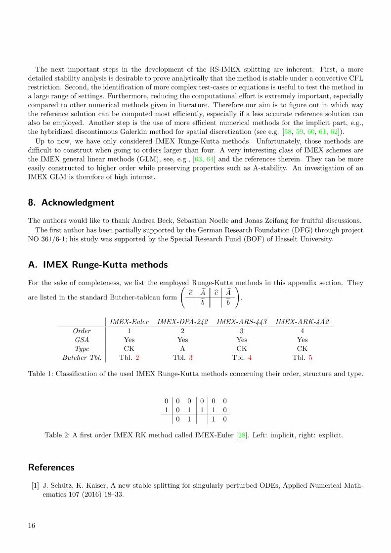
Table 1: Classification of the used IMEX Runge-Kutta methods concerning their order, structure and type.

0 0 0 0 0 01 0 1 1 1 0

0 1 1 0

Table 2: A first order IMEX RK method called IMEX-Euler [28]. Left: implicit, right: explicit.

References

[1] J. Schutz, K. Kaiser, A new stable splitting for singularly perturbed ODEs, Applied Numerical Math-ematics 107 (2016) 18–33.

16

1/2 1/2 0 0 0 0 0 0 0 02/3 1/6 1/2 0 0 1/3 1/3 0 0 01/2 -1/2 1/2 1/2 0 1 1 0 0 01 3/2 -3/2 1/2 1/2 1 1/2 0 1/2 0

3/2 -3/2 1/2 1/2 1/2 0 1/2 0

Table 3: A second order IMEX RK method called IMEX-DPA-242 [33]. Left: implicit, right: explicit.

0 0 0 0 0 0 0 0 0 0 0 01/2 0 1/2 0 0 0 1/2 1/2 0 0 0 02/3 0 1/6 1/2 0 0 2/3 11/18 1/18 0 0 01/2 0 -1/2 1/2 1/2 0 1/2 5/6 -5/6 1/2 0 01 0 3/2 -3/2 1/2 1/2 1 1/4 7/4 3/4 -7/4 0

0 3/2 -3/2 1/2 1/2 1/4 7/4 3/4 -7/4 0

Table 4: A third order IMEX RK method called IMEX-ARS-443[28]. Left: implicit, right: explicit.

[2] K. Kaiser, J. Schutz, R. Schobel, S. Noelle, A new stable splitting for the isentropic Euler equations,Journal of Scientific Computing (in press).URL https://www.igpm.rwth-aachen.de/forschung/preprints/442

[3] J. D. Anderson, Fundamentals of Aerodynamics, 3rd Edition, McGraw-Hill New York, 2001.

[4] P. Wesseling, Principles of Computational Fluid Dynamics, Vol. 29 of Springer Series in ComputationalMechanics, Springer Verlag, 2001.

[5] S. Klainerman, A. Majda, Singular limits of quasilinear hyperbolic systems with large parameters andthe incompressible limit of compressible fluids, Communications on Pure and Applied Mathematics 34(1981) 481–524.

[6] S. Schochet, Fast singular limits of hyperbolic PDEs, Journal of Differential Equations 114 (2) (1994)476–512.

[7] W.-A. Yong, A note on the zero Mach number limit of compressible Euler equations, Proceedings ofthe American Mathematical Society 133 (10) (2005) 3079–3085.

[8] D. Kroner, Numerical Schemes for Conservation Laws, Wiley Teubner, 1997.

[9] G. Bispen, M. Lukacova-Medvid’ova, L. Yelash, Asymptotic preserving IMEX finite volume schemesfor low mach number euler equations with gravitation, Journal of Computational Physics 335 (2017)222–248.

0 0 0 0 0 0 0 0 0 0 0 0 0 0 0 01/3 -1/6 1/2 0 0 0 0 0 1/3 1/3 0 0 0 0 0 01/3 1/6 -1/3 1/2 0 0 0 0 1/3 1/6 1/6 0 0 0 0 01/2 3/8 -3/8 0 1/2 0 0 0 1/2 1/8 0 3/8 0 0 0 01/2 1/8 0 3/8 -1/2 1/2 0 0 1/2 1/8 0 3/8 0 0 0 01 -1/2 0 3 -3 1 1/2 0 1 1/2 0 -3/2 0 2 0 01 1/6 0 0 0 2/3 -1/2 2/3 1 1/6 0 0 0 2/3 1/6 0

1/6 0 0 0 2/3 -1/2 2/3 1/6 0 0 0 2/3 1/6 0

Table 5: A fourth order IMEX RK method called IMEX-ARK-4A2[34]. Left: implicit, right: explicit.

17

[10] G. Bispen, K. Arun, M. Lukacova-Medvid’ova, S. Noelle, IMEX large time step finite volume methodsfor low Froude number shallow water flows, Communications in Computational Physics 16 (2014) 307–347.

[11] F. Cordier, P. Degond, A. Kumbaro, An asymptotic-preserving all-speed scheme for the Euler andNavier-Stokes equations, Journal of Computational Physics 231 (2012) 5685–5704.

[12] P. Degond, M. Tang, All speed scheme for the low Mach number limit of the isentropic Euler equation,Communications in Computational Physics 10 (2011) 1–31.

[13] F. Giraldo, M. Restelli, M. Lauter, Semi-implicit formulations of the Navier-Stokes equations: Appli-cation to nonhydrostatic atmospheric modeling, SIAM Journal on Scientific Computing 32 (6) (2010)3394–3425.

[14] J. Haack, S. Jin, J.-G. Liu, An all-speed asymptotic-preserving method for the isentropic Euler andNavier-Stokes equations, Communications in Computational Physics 12 (2012) 955–980.

[15] R. Klein, Semi-implicit extension of a Godunov-type scheme based on low Mach number asymptoticsI: One-dimensional flow, Journal of Computational Physics 121 (1995) 213–237.

[16] A. Muller, J. Behrens, F. Giraldo, V. Wirth, Comparison between adaptive and uniform discontinuousGalerkin simulations in dry 2d bubble experiments, Journal of Computational Physics 235 (2013) 371–393.

[17] S. Noelle, G. Bispen, K. Arun, M. Lukacova-Medvid’ova, C.-D. Munz, A weakly asymptotic preserv-ing low Mach number scheme for the Euler equations of gas dynamics, SIAM Journal on ScientificComputing 36 (2014) B989–B1024.

[18] M. Restelli, Semi-lagrangian and semi-implicit discontinuous Galerkin methods for atmospheric mod-eling applications, PhD thesis Politecnico di Milano.

[19] L. Yelash, A. Muller, M. Lukacova-Medvid’ova, F. X. Giraldo, V. Wirth, Adaptive discontinuousevolution Galerkin method for dry atmospheric flow, Journal of Computational Physics 268 (2014)106–133.

[20] J. Schutz, S. Noelle, Flux splitting for stiff equations: A notion on stability, Journal of ScientificComputing 64 (2) (2015) 522–540.

[21] H. Zakerzadeh, S. Noelle, A note on the stability of implicit-explicit flux splittings for stiff hyperbolicsystems, IGPM Preprint Nr. 449.

[22] F. X. Giraldo, M. Restelli, High-order semi-implicit time-integrators for a triangular discontinuousGalerkin oceanic shallow water model, International Journal for Numerical Methods in Fluids 63 (9)(2010) 1077–1102.

[23] F. Filbet, S. Jin, A class of asymptotic-preserving schemes for kinetic equations and related problemswith stiff sources, Journal of Computational Physics 229 (20) (2010) 7625–7648.

[24] H. Zakerzadeh, Asymptotic analysis of the RS-IMEX scheme for the shallow water equations in onespace dimension, IGPM Preprint Nr. 455.

[25] U. M. Ascher, S. Ruuth, B. Wetton, Implicit-Explicit methods for time-dependent partial differentialequations, SIAM Journal on Numerical Analysis 32 (1995) 797–823.

18

[26] W. Hundsdorfer, J. Jaffre, Implicit–explicit time stepping with spatial discontinuous finite elements,Applied Numerical Mathematics 45 (2) (2003) 231–254.

[27] W. Hundsdorfer, S.-J. Ruuth, IMEX extensions of linear multistep methods with general monotonicityand boundedness properties, Journal of Computational Physics 225 (2) (2007) 2016–2042.

[28] U. M. Ascher, S. Ruuth, R. Spiteri, Implicit-explicit Runge-Kutta methods for time-dependent partialdifferential equations, Applied Numerical Mathematics 25 (1997) 151–167.

[29] S. Boscarino, L. Pareschi, G. Russo, Implicit-explicit Runge–Kutta schemes for hyperbolic systems andkinetic equations in the diffusion limit, SIAM Journal on Scientific Computing 35 (1) (2013) A22–A51.

[30] C. A. Kennedy, M. H. Carpenter, Additive Runge-Kutta schemes for convection-diffusion-reaction equa-tions, Applied Numerical Mathematics 44 (2003) 139–181.

[31] L. Pareschi, G. Russo, Implicit-explicit Runge-Kutta schemes for stiff systems of differential equations,Recent Trends in Numerical Analysis 3 (2000) 269–289.

[32] G. Russo, S. Boscarino, IMEX Runge-Kutta schemes for hyperbolic systems with diffusive relaxation,European Congress on Computational Methods in Applied Sciences and Engineering (ECCOMAS2012).

[33] G. Dimarco, L. Pareschi, Asymptotic preserving implicit-explicit Runge–Kutta methods for nonlinearkinetic equations, SIAM Journal on Numerical Analysis 51 (2) (2013) 1064–1087.

[34] H. Liu, J. Zou, Some new additive Runge–Kutta methods and their applications, Journal of Computa-tional and Applied Mathematics 190 (1-2) (2006) 74–98.

[35] B. Cockburn, S. Hou, C.-W. Shu, The Runge–Kutta local projection discontinuous Galerkin finiteelement method for conservation laws IV: The multidimensional case, Mathematics of Computation 54(1990) 545–581.

[36] B. Cockburn, S. Y. Lin, C.-W. Shu, TVB Runge-Kutta local projection discontinuous Galerkin finiteelement method for conservation laws III: One dimensional systems, Journal of Computational Physics84 (1989) 90–113.

[37] B. Cockburn, C.-W. Shu, TVB Runge-Kutta local projection discontinuous Galerkin finite elementmethod for conservation laws II: General framework, Mathematics of Computation 52 (1988) 411–435.

[38] B. Cockburn, C.-W. Shu, The Runge-Kutta local projection p1-discontinuous Galerkin finite elementmethod for scalar conservation laws, RAIRO Mathematical modelling and numerical analysis 25 (1991)337–361.

[39] B. Cockburn, C.-W. Shu, The Runge-Kutta discontinuous Galerkin Method for conservation laws V:Multidimensional Systems, Mathematics of Computation 141 (1998) 199–224.

[40] A. Kanevsky, M. H. Carpenter, D. Gottlieb, J. S. Hesthaven, Application of implicit-explicit high orderRunge-Kutta methods to discontinuous-Galerkin schemes, Journal of Computational Physics 225 (2)(2007) 1753–1781.

[41] P.-O. Persson, High-order LES simulations using implicit-explicit Runge-Kutta schemes, AIAA Paper11-684 (2011).

19

[42] H. Wang, C.-W. Shu, Q. Zhang, Stability and error estimates of local discontinuous Galerkin meth-ods with implicit-explicit time-marching for advection-diffusion problems, SIAM Journal on NumericalAnalysis 53 (1) (2015) 206–227.

[43] S. Jin, Asymptotic preserving (AP) schemes for multiscale kinetic and hyperbolic equations: A review,Rivista di Matematica della Universita Parma 3 (2012) 177–216.

[44] S. Boscarino, Error analysis of IMEX Runge-Kutta methods derived from differential-algebraic systems,SIAM Journal on Numerical Analysis 45 (2007) 1600–1621.

[45] H. Guillard, C. Viozat, On the behavior of upwind schemes in the low Mach number limit, Computersand Fluids 28 (1) (1999) 63–86.

[46] E. Turkel, Preconditioned methods for solving the incompressible and low speed compressible equations,Journal of Computational Physics 72 (2) (1987) 277 – 298.

[47] D. D. Pietro, A. Ern, Mathematical aspects of discontinuous Galerkin Methods, Vol. 69, SpringerScience & Business Media, 2011.

[48] G. Bispen, IMEX finite volume methods for the shallow water equations, Ph.D. thesis, JohannesGutenberg-Universitat (2015).

[49] B. Schling, The Boost C++ Libraries, XML Press, 2011.

[50] BOOST C++ Libraries, http://www.boost.org.

[51] J. Schoberl, Netgen - an advancing front 2d/3d-mesh generator based on abstract rules, Computingand Visualization in Science 1 (1997) 41–52.

[52] S. Balay, W. D. Gropp, L. C. McInnes, B. F. Smith, Efficient management of parallelism in objectoriented numerical software libraries, in: E. Arge, A. M. Bruaset, H. P. Langtangen (Eds.), ModernSoftware Tools in Scientific Computing, Birkhauser Press Boston, 1997, pp. 163–202.

[53] S. Balay, J. Brown, K. Buschelman, W. D. Gropp, D. Kaushik, M. G. Knepley, L. C. McInnes, B. F.Smith, H. Zhang, PETSc Web page, http://www.mcs.anl.gov/petsc (2011).

[54] S. Balay, J. Brown, K. Buschelman, V. Eijkhout, W. D. Gropp, D. Kaushik, M. G. Knepley, L. C.McInnes, B. F. Smith, H. Zhang, PETSc users manual, Tech. Rep. ANL-95/11 - Revision 3.1, ArgonneNational Laboratory (2010).

[55] B. Cockburn, C. W. Shu, Runge-Kutta discontinuous Galerkin methods for convection-dominated prob-lems, Journal of Scientific Computing 16 (2001) 173–261.

[56] J. Sesterhenn, B. Muller, H. Thomann, On the cancellation problem in calculating compressible lowmach number flows, Journal of Computational Physics 151 (2) (1999) 597 – 615. doi:http://dx.doi.org/10.1006/jcph.1999.6211.URL http://www.sciencedirect.com/science/article/pii/S0021999199962113

[57] S.-H. Lee, Cancellation problem of preconditioning method at low mach numbers, Journal of Compu-tational Physics 225 (2) (2007) 1199 – 1210. doi:http://dx.doi.org/10.1016/j.jcp.2007.04.001.URL http://www.sciencedirect.com/science/article/pii/S0021999107001544

[58] N. Nguyen, J. Peraire, B. Cockburn, A hybridizable discontinuous Galerkin method for the incompress-ible navier-stokes equations, AIAA Paper 2010-362.

20

[59] J. Peraire, N. C. Nguyen, B. Cockburn, A hybridizable discontinuous Galerkin method for the com-pressible Euler and Navier-Stokes equations, AIAA Paper 10-363 (2010).

[60] A. Jaust, J. Schutz, M. Woopen, An HDG method for unsteady compressible flows, in: R. M. Kirby,M. Berzins, J. S. Hesthaven (Eds.), Spectral and High Order Methods for Partial Differential EquationsICOSAHOM 2014, Vol. 106 of Lecture Notes in Computational Science and Engineering, SpringerInternational Publishing, 2015, pp. 267–274.

[61] A. Jaust, J. Schutz, M. Woopen, A hybridized discontinuous Galerkin method for unsteady flows withshock-capturing, AIAA Paper 2014-2781.

[62] J. Schutz, M. Woopen, G. May, A hybridized DG/mixed scheme for nonlinear advection-diffusionsystems, including the compressible Navier-Stokes equations, AIAA Paper 2012-0729.

[63] P. E. Vos, C. Eskilsson, A. Bolis, S. Chun, R. M. Kirby, S. J. Sherwin, A generic framework for time-stepping partial differential equations (PDEs): general linear methods, object-oriented implementationand application to fluid problems, International Journal of Computational Fluid Dynamics 25 (3) (2011)107–125.

[64] H. Zhang, A. Sandu, S. Blaise, Partitioned and implicit–explicit general linear methods for ordi-nary differential equations, Journal of Scientific Computing 61 (1) (2014) 119–144. doi:10.1007/

s10915-014-9819-z.URL http://dx.doi.org/10.1007/s10915-014-9819-z

21