A Hardware Implementation of the SoftOutput Viterbi Algorithm for Serially

Concatenated Convolutional Codes

by

Brett W. Werling

Submitted to the graduate degree program in ElectricalEngineering and Computer Science and the Graduate Faculty

of the University of Kansas in partial fulfillment of therequirements for the degree of Master of Science.

Thesis Committee:

Dr. Erik Perrins: Chairperson

Dr. Andrew Gill

Dr. Perry Alexander

Date Defended

The Thesis Committee for Brett W. Werling certifiesthat this is the approved version of the following thesis:

A Hardware Implementation of the Soft Output Viterbi Algorithm for SeriallyConcatenated Convolutional Codes

Committee:

Chairperson

Date Approved

ii

Acknowledgements

I would like to thank Dr. Erik Perrins for giving me the opportunity to work onthis project and also for introducing me to the wonderful world of error control coding.Without his support, none of this would have been possible. I would also like to thankDr. Andrew Gill and Dr. Perry Alexander for taking time to serve on my committee,as well as everyone at KU who has helped me over the years. Finally, I would like tothank my family for all their love, support, and for always believing in me.

iii

Abstract

This thesis outlines the hardware design of a soft output Viterbi algorithm decoderfor use in a serially concatenated convolutional code system. Convolutional codes andtheir related structures are described, as well as the algorithms used to decode them. Adecoder design intended for a field-programmable gate array is presented. Simulationsof the proposed design are compared with simulations of a software reference decoderthat is known to be correct. Results of the simulations are shown and interpreted, andsuggestions for future improvements are given.

iv

Contents

Acceptance Page ii

Acknowledgements iii

Abstract iv

1 Introduction 11.1 Background . . . . . . . . . . . . . . . . . . . . . . . . . . . . . . . . 11.2 Objectives . . . . . . . . . . . . . . . . . . . . . . . . . . . . . . . . . 21.3 Organization . . . . . . . . . . . . . . . . . . . . . . . . . . . . . . . . 2

2 Convolutional Codes 42.1 Overview . . . . . . . . . . . . . . . . . . . . . . . . . . . . . . . . . 42.2 Convolutional Encoders . . . . . . . . . . . . . . . . . . . . . . . . . . 52.3 Trellis Structure . . . . . . . . . . . . . . . . . . . . . . . . . . . . . . 6

3 Channel Models 93.1 Binary Symmetric Channel . . . . . . . . . . . . . . . . . . . . . . . . 93.2 Additive White Gaussian Noise Channel . . . . . . . . . . . . . . . . . 11

4 Decoding Convolutional Codes 134.1 Viterbi Algorithm . . . . . . . . . . . . . . . . . . . . . . . . . . . . . 13

4.1.1 Forward Loop . . . . . . . . . . . . . . . . . . . . . . . . . . . 144.1.2 Backward Loop . . . . . . . . . . . . . . . . . . . . . . . . . . 18

4.2 Soft Output Viterbi Algorithm . . . . . . . . . . . . . . . . . . . . . . 19

5 Serially Concatenated Convolutional Codes 25

v

6 Hardware Implementation 286.1 Design . . . . . . . . . . . . . . . . . . . . . . . . . . . . . . . . . . . 28

6.1.1 Code and Trellis . . . . . . . . . . . . . . . . . . . . . . . . . 286.1.2 Inputs and Outputs . . . . . . . . . . . . . . . . . . . . . . . . 296.1.3 Decoder Structure . . . . . . . . . . . . . . . . . . . . . . . . 326.1.4 Overflow Handling . . . . . . . . . . . . . . . . . . . . . . . . 32

6.2 Metric Manager . . . . . . . . . . . . . . . . . . . . . . . . . . . . . . 346.2.1 Metric Calculator . . . . . . . . . . . . . . . . . . . . . . . . . 34

6.3 Hard-Decision Traceback Unit . . . . . . . . . . . . . . . . . . . . . . 366.4 Reliability Traceback Unit . . . . . . . . . . . . . . . . . . . . . . . . 396.5 Output Calculator . . . . . . . . . . . . . . . . . . . . . . . . . . . . . 41

7 Performance Results 447.1 Comparison with Software Reference . . . . . . . . . . . . . . . . . . 447.2 Hardware Performance . . . . . . . . . . . . . . . . . . . . . . . . . . 51

8 Conclusion 538.1 Interpretation of Results . . . . . . . . . . . . . . . . . . . . . . . . . 538.2 Suggested Improvements . . . . . . . . . . . . . . . . . . . . . . . . . 54

References 55

vi

List of Figures

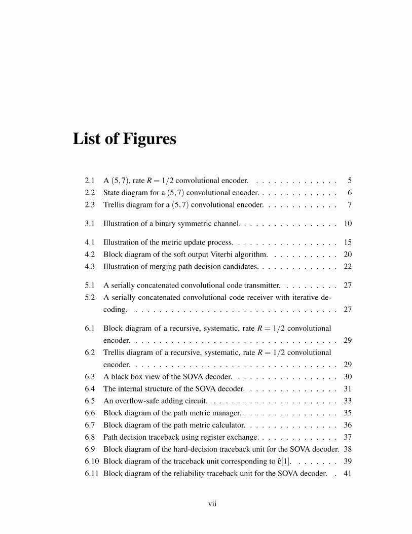
2.1 A (5,7), rate R = 1/2 convolutional encoder. . . . . . . . . . . . . . . 52.2 State diagram for a (5,7) convolutional encoder. . . . . . . . . . . . . . 62.3 Trellis diagram for a (5,7) convolutional encoder. . . . . . . . . . . . . 7

3.1 Illustration of a binary symmetric channel. . . . . . . . . . . . . . . . . 10

4.1 Illustration of the metric update process. . . . . . . . . . . . . . . . . . 154.2 Block diagram of the soft output Viterbi algorithm. . . . . . . . . . . . 204.3 Illustration of merging path decision candidates. . . . . . . . . . . . . . 22

5.1 A serially concatenated convolutional code transmitter. . . . . . . . . . 275.2 A serially concatenated convolutional code receiver with iterative de-

coding. . . . . . . . . . . . . . . . . . . . . . . . . . . . . . . . . . . 27

6.1 Block diagram of a recursive, systematic, rate R = 1/2 convolutionalencoder. . . . . . . . . . . . . . . . . . . . . . . . . . . . . . . . . . . 29

6.2 Trellis diagram of a recursive, systematic, rate R = 1/2 convolutionalencoder. . . . . . . . . . . . . . . . . . . . . . . . . . . . . . . . . . . 29

6.3 A black box view of the SOVA decoder. . . . . . . . . . . . . . . . . . 306.4 The internal structure of the SOVA decoder. . . . . . . . . . . . . . . . 316.5 An overflow-safe adding circuit. . . . . . . . . . . . . . . . . . . . . . 336.6 Block diagram of the path metric manager. . . . . . . . . . . . . . . . . 356.7 Block diagram of the path metric calculator. . . . . . . . . . . . . . . . 366.8 Path decision traceback using register exchange. . . . . . . . . . . . . . 376.9 Block diagram of the hard-decision traceback unit for the SOVA decoder. 386.10 Block diagram of the traceback unit corresponding to c[1]. . . . . . . . 396.11 Block diagram of the reliability traceback unit for the SOVA decoder. . 41

vii

6.12 Block diagram of the traceback unit corresponding to z[1]. . . . . . . . 426.13 Block diagram of a reliability update unit. . . . . . . . . . . . . . . . . 436.14 Block diagram of the output calculator. . . . . . . . . . . . . . . . . . . 43

7.1 Plot of simulated bit error rate for B = 6, T = 8. . . . . . . . . . . . . . 467.2 Plot of simulated bit error rate for B = 7, T = 8. . . . . . . . . . . . . . 467.3 Plot of simulated bit error rate for B = 8, T = 8. . . . . . . . . . . . . . 477.4 Plot of simulated bit error rate for B = 9, T = 8. . . . . . . . . . . . . . 477.5 Plot of simulated bit error rate for B = 6, T = 16. . . . . . . . . . . . . 487.6 Plot of simulated bit error rate for B = 7, T = 16. . . . . . . . . . . . . 487.7 Plot of simulated bit error rate for B = 8, T = 16. . . . . . . . . . . . . 497.8 Plot of simulated bit error rate for B = 9, T = 16. . . . . . . . . . . . . 49

viii

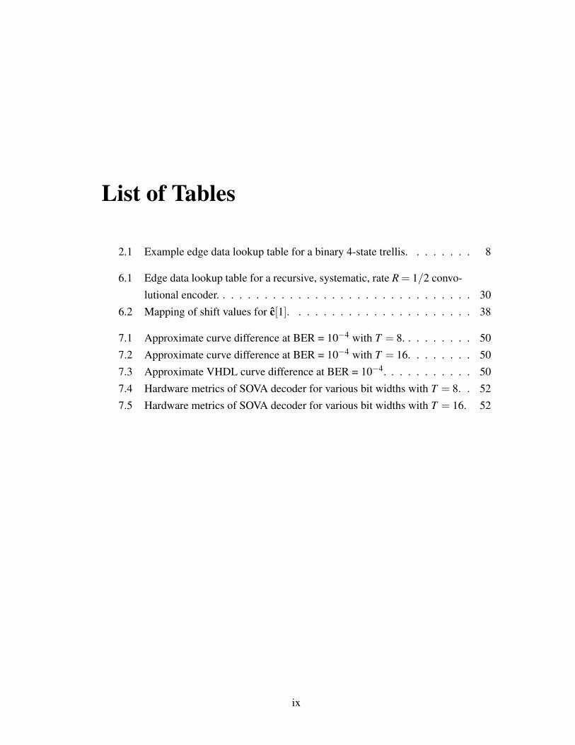
List of Tables

2.1 Example edge data lookup table for a binary 4-state trellis. . . . . . . . 8

6.1 Edge data lookup table for a recursive, systematic, rate R = 1/2 convo-lutional encoder. . . . . . . . . . . . . . . . . . . . . . . . . . . . . . . 30

6.2 Mapping of shift values for c[1]. . . . . . . . . . . . . . . . . . . . . . 38

7.1 Approximate curve difference at BER = 10−4 with T = 8. . . . . . . . . 507.2 Approximate curve difference at BER = 10−4 with T = 16. . . . . . . . 507.3 Approximate VHDL curve difference at BER = 10−4. . . . . . . . . . . 507.4 Hardware metrics of SOVA decoder for various bit widths with T = 8. . 527.5 Hardware metrics of SOVA decoder for various bit widths with T = 16. 52

ix

Chapter 1

Introduction

1.1 Background

Forward error correction (FEC) codes have long been a powerful tool in the ad-

vancement of information storage and transmission. By introducing meaningful redun-

dancy (FEC codes) into a stream of information, systems gain the ability to not only

detect data errors, but also correct them. With this ability, the systems can run on less

power, operate at longer distances, and decrease the need for costly retransmissions.

As the world of aeronautical telemetry looks to improve upon its current communi-

cation methods, its need for FEC codes becomes clear. The Information and Telecom-

munication Technology Center (ITTC) at the University of Kansas is involved with a

project to develop such codes and produce hardware prototypes for testing purposes.

The High-Rate High-Speed Forward Error Correction Architectures for Aeronautical

Telemetry (HFEC) project is currently investigating the benefits of two types of FEC

codes, as well as the methods with which they are built in hardware. One of these

codes, a serially concatenated convolutional code (SCCC), was developed at ITTC by

Dr. Erik Perrins, and its internal components are the focus of this thesis.

1

1.2 Objectives

Both of the decoding blocks contained in an SCCC decoder employ the soft output

Viterbi algorithm (SOVA). Though much testing of this algorithm has been performed

in software on general purpose processors, there is a need for a SOVA decoder circuit

design which can be used throughout the remainder of the HFEC project. The work

presented in this paper focuses on an initial design for a SOVA decoder that can be

run on a field-programmable gate array (FPGA), written in the widely-used hardware

description language known as VHDL.

1.3 Organization

This thesis is organized into 8 chapters. The information contained in these chapters

is listed below (chapters containing the novel contributions of this thesis are marked

with a *):

• Chapter 2 gives a description of convolutional codes and the structures associated

with them.

• Chapter 3 gives an overview of two of the important channel models used when

evaluating the performance of convolutional codes.

• Chapter 4 gives a detailed description of the algorithms used to decode convolu-

tional codes.

• Chapter 5 explains how the decoding algorithms of Chapter 4 fit into the SCCC

system.

• *Chapter 6 gives a highly-detailed look at a hardware design of a SOVA decoder

2

for use in the HFEC project. This chapter contains the majority of the work of

this thesis, and therefore is longer.

• *Chapter 7 reveals the results of the implementation of the SOVA decoder in

VHDL.

• Chapter 8 gives conclusions and suggestions for future improvements.

3

Chapter 2

Convolutional Codes

This chapter focuses on the structure and utility of convolutional codes. Much of

the information contained in this chapter is drawn from [1], which discusses these codes

in great detail. Additional references are cited as needed.

2.1 Overview

Convolutional codes are a class of linear codes whose encoding operation can be

viewed as a filtering process. The name convolutional codes comes from the mathe-

matical backbone of any digital filter: linear convolution. Convolutional encoders are

typically nothing more than a set of binary digital filters whose outputs are interleaved

into a single encoded stream. This allows convolutional encoders to have very low

complexity, while the structure of the code maintains the high performance desired in

most applications.

The coding rate R for any coded system is defined as R= k/n, where k is the number

of input symbols and n is the number of output symbols. Though some convolutional

codes may share the same value of R as a particular linear block code, they usually

4

D D

+

+

mK

mK-1 m

K-2

cK[1]

cK[0]

cK

[101]

[111]

5

7

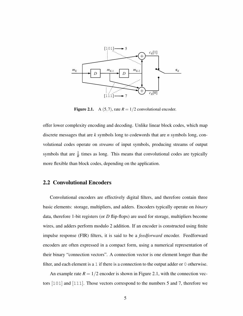
Figure 2.1. A (5,7), rate R = 1/2 convolutional encoder.

offer lower complexity encoding and decoding. Unlike linear block codes, which map

discrete messages that are k symbols long to codewords that are n symbols long, con-

volutional codes operate on streams of input symbols, producing streams of output

symbols that are 1R times as long. This means that convolutional codes are typically

more flexible than block codes, depending on the application.

2.2 Convolutional Encoders

Convolutional encoders are effectively digital filters, and therefore contain three

basic elements: storage, multipliers, and adders. Encoders typically operate on binary

data, therefore 1-bit registers (or D flip-flops) are used for storage, multipliers become

wires, and adders perform modulo 2 addition. If an encoder is constructed using finite

impulse response (FIR) filters, it is said to be a feedforward encoder. Feedforward

encoders are often expressed in a compact form, using a numerical representation of

their binary “connection vectors”. A connection vector is one element longer than the

filter, and each element is a 1 if there is a connection to the output adder or 0 otherwise.

An example rate R = 1/2 encoder is shown in Figure 2.1, with the connection vec-

tors [101] and [111]. Those vectors correspond to the numbers 5 and 7, therefore we

5

11

00

0110

0/00

1/01

0/01

1/00

mK−2, mK−1

mK

/ cK

Figure 2.2. State diagram for a (5,7) convolutional encoder.

call it a (5,7) convolutional encoder. The input stream m is filtered to produce the out-

put streams c[1] and c[0], which are then interleaved to produce the final output stream

c. Each mK contains one bit, therefore each cK has two bits. This results in a rate

R = 1/2 code. It is necessary to point out that cK[i] represents bit i in the vector cK ,

indexing in ascending order from right to left. For example, if cK = 10, then cK[1] = 1

and cK[0] = 0. This notation will be used for the remainder of the document.

2.3 Trellis Structure

Since convolutional encoders contain memory, they can be thought of as having a

state at any time throughout the encoding process. In other words, a convolutional en-

coder is a state machine and can be visualized with a state diagram, which shows how

all possible inputs affect both the output and next state of the encoder. The (5,7) en-

coder shown in Figure 2.1 contains two 1-bit registers, therefore the value representing

its state is 2-bits wide. We assume that the register storing mK−2 is the most significant

bit (MSB) of the state and the register storing mK−1 is the least significant bit (LSB)

6

0/00

1/01

qS qE

0

2

3

1

0

2

3

1

e

0

1

2

3

4

5

6

7

m(e) / c(e)

(00)

(01)

(10)

(11)

(00)

(01)

(10)

(11)

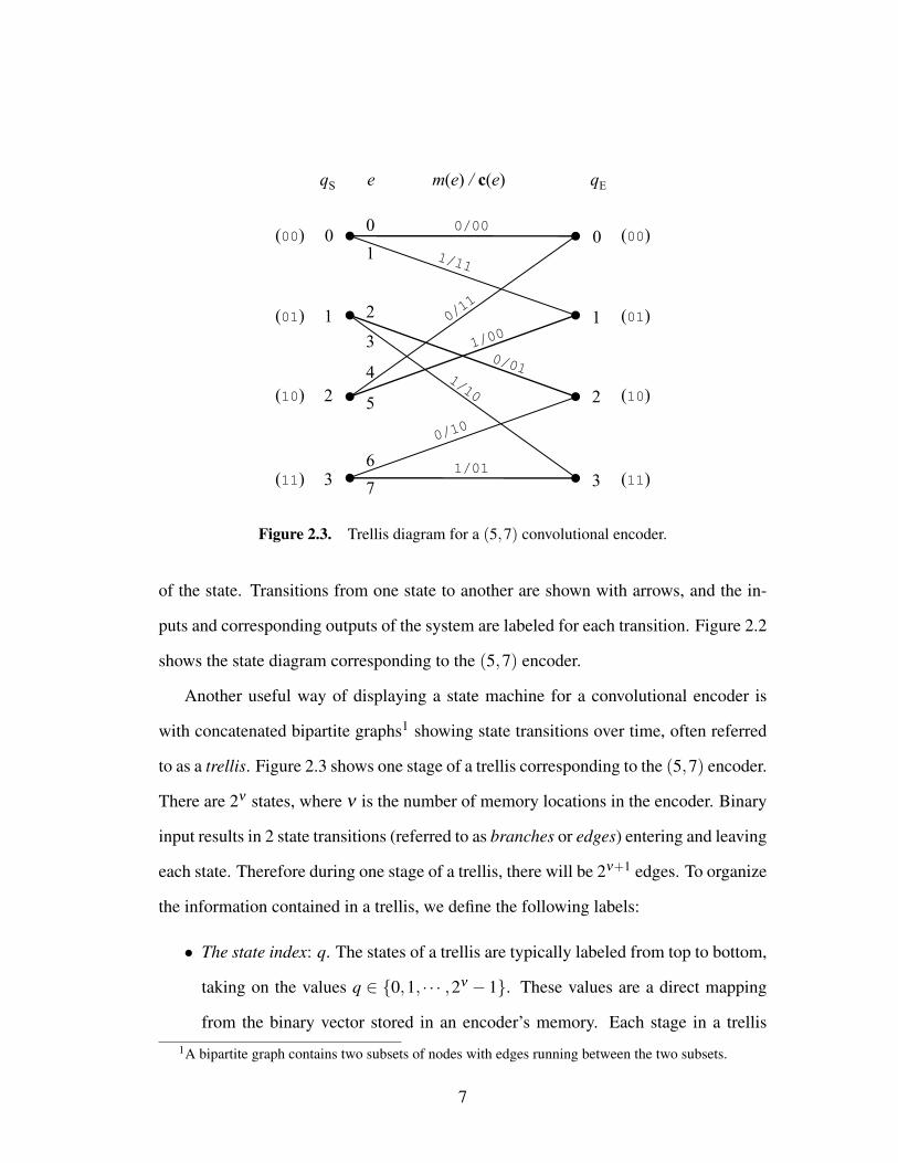
Figure 2.3. Trellis diagram for a (5,7) convolutional encoder.

of the state. Transitions from one state to another are shown with arrows, and the in-

puts and corresponding outputs of the system are labeled for each transition. Figure 2.2

shows the state diagram corresponding to the (5,7) encoder.

Another useful way of displaying a state machine for a convolutional encoder is

with concatenated bipartite graphs1 showing state transitions over time, often referred

to as a trellis. Figure 2.3 shows one stage of a trellis corresponding to the (5,7) encoder.

There are 2ν states, where ν is the number of memory locations in the encoder. Binary

input results in 2 state transitions (referred to as branches or edges) entering and leaving

each state. Therefore during one stage of a trellis, there will be 2ν+1 edges. To organize

the information contained in a trellis, we define the following labels:

• The state index: q. The states of a trellis are typically labeled from top to bottom,

taking on the values q ∈ {0,1, · · · ,2ν − 1}. These values are a direct mapping

from the binary vector stored in an encoder’s memory. Each stage in a trellis1A bipartite graph contains two subsets of nodes with edges running between the two subsets.

7

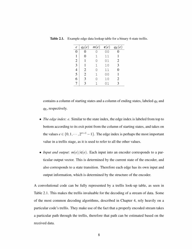
Table 2.1. Example edge data lookup table for a binary 4-state trellis.

e qS(e) m(e) c(e) qE(e)0 0 0 00 01 0 1 11 12 1 0 01 23 1 1 10 34 2 0 11 05 2 1 00 16 3 0 10 27 3 1 01 3

contains a column of starting states and a column of ending states, labeled qS and

qE, respectively.

• The edge index: e. Similar to the state index, the edge index is labeled from top to

bottom according to its exit point from the column of starting states, and takes on

the values e∈ {0,1, · · · ,2ν+1−1}. The edge index is perhaps the most important

value in a trellis stage, as it is used to refer to all the other values.

• Input and output: m(e)/c(e). Each input into an encoder corresponds to a par-

ticular output vector. This is determined by the current state of the encoder, and

also corresponds to a state transition. Therefore each edge has its own input and

output information, which is determined by the structure of the encoder.

A convolutional code can be fully represented by a trellis look-up table, as seen in

Table 2.1. This makes the trellis invaluable for the decoding of a stream of data. Some

of the most common decoding algorithms, described in Chapter 4, rely heavily on a

particular code’s trellis. They make use of the fact that a properly encoded stream takes

a particular path through the trellis, therefore that path can be estimated based on the

received data.

8

Chapter 3

Channel Models

In any communications system, it is important to understand how a signal is af-

fected by the transmission channel it encounters. This chapter focuses on two common

models for communcation channels that are used when evaluating the performance of

convolutional codes.

3.1 Binary Symmetric Channel

The binary symmetric channel (BSC) is a channel model that involves only the

transmission of bits, defining a hard line to determine between a 0 or 1. For each unit

of time, a bit is transmitted with probability of error p and probability of success 1− p.

The value p is know as the crossover probability, because it represents the probability

that a bit “crosses over” from 0 to 1 or 1 to 0, which can be seen in Figure 3.1. A BSC

transmission can be modeled as

r = s⊕n, (3.1)

where r contains received bits, s contains transmitted bits, and n contains possible bit

errors. The sequences r, s, and n have the same length and are indexed in discrete-time

9

p

1 − p

1 − p

p

0

1

0

1

transmit receive

Figure 3.1. Illustration of a binary symmetric channel.

by i. If there is a bit error at time i, ni will be 1, otherwise it is 0. The sequence n is an

independent and identically distributed Bernoulli random process. The⊕ operator, also

known as xor, applies any bit error at ni by toggling the value of si. In other words, ⊕

corresponds to modulo 2 addition.

When using a BSC model, the comparison between a transmitted sequence and a

received sequence is most often done using Hamming distance. The Hamming dis-

tance between the sequences s and r is defined as the number of positions in which the

corresponding elements are different. This is expressed mathematically as

dH(s,r) =n−1

∑i=0

[s[i] 6= r[i]], (3.2)

where

[si 6= ri] =

1 if si 6= ri

0 if si = ri.

When a sequence is received over a BSC, it is compared with a group of possible

transmitted sequences to determine which one it most closely resembles. Typically, the

winner is the one with the shortest Hamming distance to the received sequence.

10

3.2 Additive White Gaussian Noise Channel

The additive white Gaussian noise (AWGN) channel is one of the most common

mathematical models for a communication channel. As the name suggests, it assumes

that a communcation link is primarily affected by Gaussian noise [2]. The AWGN

model can be applied to many physical channels, which makes it very useful when

evaluating the performance of a system.

In order for a data sequence to be physically transmitted, it must encounter some

form of modulation. One simple modulation scheme is binary phase-shift keying (BPSK),

where bits are mapped to antipodal values (+A or−A), with 0→ (−A) and 1→ (+A).

Once a bit sequence has been modulated, it is sent over the channel, where it encounters

additive Gaussian noise. A mathematical representation of this is

r = s+n, (3.3)

where r contains noisy received values, s contains transmitted antipodal bit values, and

n contains noise values. This is similar to the BSC model in Equation 3.1, however each

sequence is real-valued and the + operator performs addition of reals. Each value in n

is an independent Gaussian random variable with mean µn = 0 and variance σ2n = N0

2 ,

where Es is the energy in a symbol (for BPSK, Es = A2) and N02 is the two-sided power

spectral density (PSD) of the noise [1]. It is typical to normalize the symbol energy to

Es = 1, therefore making A = 1.

The performance of a digital communication system is often quantified with the bit

error rate (BER) versus the signal-to-noise ratio (SNR). The SNR is typically defined

as Eb/N0, where Eb is the energy in an information bit. In an uncoded BPSK system,

each transmitted symbol corresponds to one information bit, or Es = Eb. In a coded

11

BPSK system, multiple transmitted symbols may correspond to a single information

bit, making the relationship dependent on the code rate R, or Es = REb. Substituting

this into the equation for the variance of the noise yields σ2n = 1

2REb/N0, assuming Es = 1.

Using the standard deviation σn to scale a standard normal (mean 0, variance 1) random

variable allows n to be generated with a desired value of Eb/N0.

When using the AWGN channel model, the optimal comparison between a transmit-

ted sequence and a received sequence is done using Euclidean distance. The squared

Euclidean distance between the sequences s and r is defined as

d2E(s,r) =

n−1

∑i=0

(s[i]− r[i])2 . (3.4)

When a sequence is received over an AWGN channel, it is compared with the set of

possible transmitted sequences to determine which one it most closely resembles. The

winner is the one that is closest in squared Euclidean distance to the received sequence.

12

Chapter 4

Decoding Convolutional Codes

This chapter describes in great detail two important algorithms for decoding convo-

lutional codes: the Viterbi algoritm and soft output Viterbi algorithm.

4.1 Viterbi Algorithm

The most common method for decoding a convolutionally-encoded sequence is the

Viterbi algorithm, which was first introduced in [3] and further analyzed in [4]. As men-

tioned in Chapter 2, the Viterbi algorithm makes use of the trellis structure to estimate

what a coded sequence might have been upon transmission. This is possible because

each coded sequence must have followed a particular path along the trellis during the

encoding process. The purpose of any convolutional decoder is to find that path so it

can decode the sequence.

An exhaustive decoding algorithm would compare the received data with every pos-

sible path along the trellis and output the one that is most likely, but that is not feasible

in most cases. The Viterbi algorithm keeps track of only the paths that occur with max-

imum likelihood (ML), which is why it is known as a maximum likelihood sequence

13

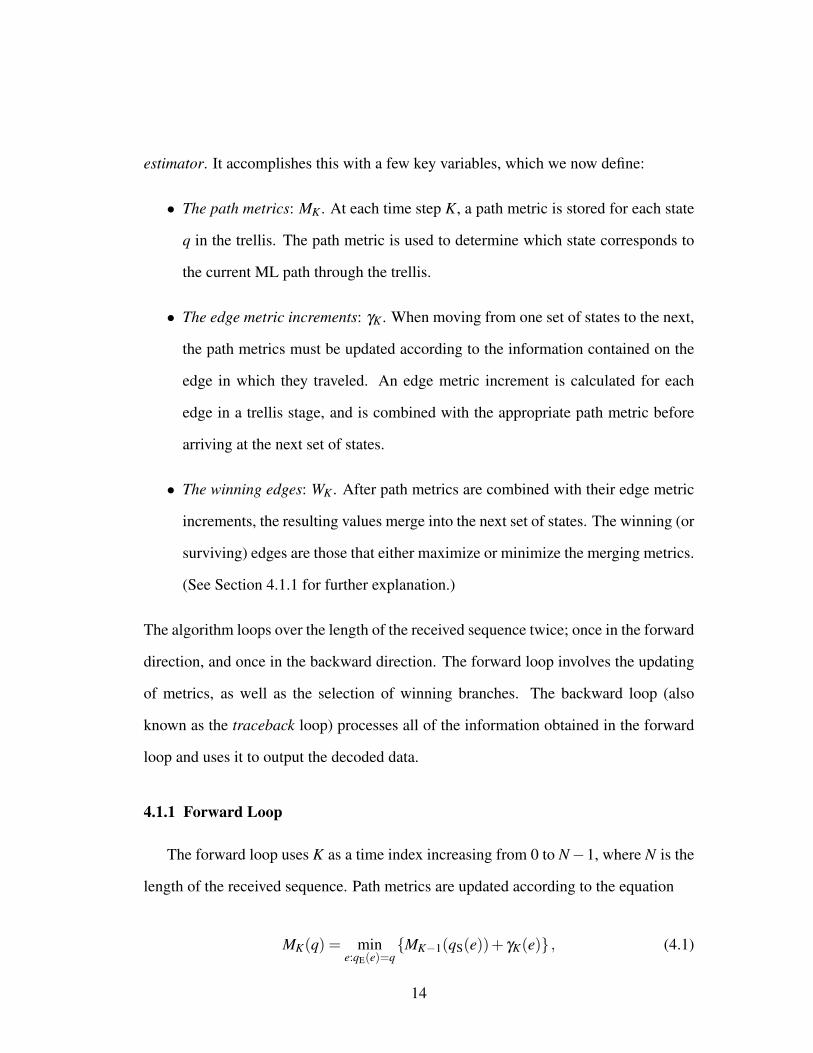
estimator. It accomplishes this with a few key variables, which we now define:

• The path metrics: MK . At each time step K, a path metric is stored for each state

q in the trellis. The path metric is used to determine which state corresponds to

the current ML path through the trellis.

• The edge metric increments: γK . When moving from one set of states to the next,

the path metrics must be updated according to the information contained on the

edge in which they traveled. An edge metric increment is calculated for each

edge in a trellis stage, and is combined with the appropriate path metric before

arriving at the next set of states.

• The winning edges: WK . After path metrics are combined with their edge metric

increments, the resulting values merge into the next set of states. The winning (or

surviving) edges are those that either maximize or minimize the merging metrics.

(See Section 4.1.1 for further explanation.)

The algorithm loops over the length of the received sequence twice; once in the forward

direction, and once in the backward direction. The forward loop involves the updating

of metrics, as well as the selection of winning branches. The backward loop (also

known as the traceback loop) processes all of the information obtained in the forward

loop and uses it to output the decoded data.

4.1.1 Forward Loop

The forward loop uses K as a time index increasing from 0 to N−1, where N is the

length of the received sequence. Path metrics are updated according to the equation

MK(q) = mine:qE(e)=q

{MK−1(qS(e))+ γK(e)} , (4.1)

14

MK

ex

ey

WK

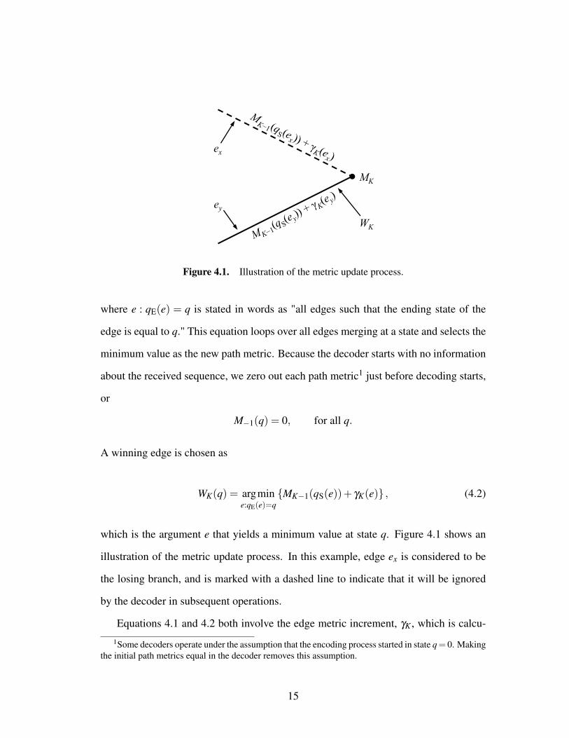
Figure 4.1. Illustration of the metric update process.

where e : qE(e) = q is stated in words as "all edges such that the ending state of the

edge is equal to q." This equation loops over all edges merging at a state and selects the

minimum value as the new path metric. Because the decoder starts with no information

about the received sequence, we zero out each path metric1 just before decoding starts,

or

M−1(q) = 0, for all q.

A winning edge is chosen as

WK(q) = argmine:qE(e)=q

{MK−1(qS(e))+ γK(e)} , (4.2)

which is the argument e that yields a minimum value at state q. Figure 4.1 shows an

illustration of the metric update process. In this example, edge ex is considered to be

the losing branch, and is marked with a dashed line to indicate that it will be ignored

by the decoder in subsequent operations.

Equations 4.1 and 4.2 both involve the edge metric increment, γK , which is calcu-

1Some decoders operate under the assumption that the encoding process started in state q= 0. Makingthe initial path metrics equal in the decoder removes this assumption.

15

lated differently according to the algorithm’s particular application. For convolutional

codes, the calculation of γK depends on the channel model being used. In a BSC, the

goal is to find a valid encoding sequence that minimizes Hamming distance with the

noisy received sequence. Therefore, the edge metric increment equation for a BSC is

γK,BSC(e) = dH(rK,c(e)), (4.3)

where rk contains noisy received bits and c(e) is the output bit vector of edge e in the

trellis.

The edge metric increment equation for an AWGN channel differs slightly from

that of a BSC in that it involves squared Euclidean distance. Equation 3.4 shows that

squared Euclidean distance is much more complex than Hamming distance, and there-

fore invites optimization. Our starting point is the equation for squared distance be-

tween rK and a(e), where rK contains noisy BPSK-mapped received symbols and a(e)

contains BPSK-mapped versions of c(e) for a particular edge (we assume BPSK for

simplicity). This is defined as

d2E(rK,a(e)) =

n−1

∑i=0

(rK[i]−a(e)[i])2

=n−1

∑i=0

rK[i]2−2rK[i]a(e)[i]+a(e)[i]2

=n−1

∑i=0

rK[i]2−2n−1

∑i=0

rK[i]a(e)[i]+n−1

∑i=0

a(e)[i]2.

Therefore the initial edge metric increment equation becomes

γ∗K,AWGN(e) =

n−1

∑i=0

rK[i]2︸ ︷︷ ︸(1)

−2n−1

∑i=0

rK[i]a(e)[i]︸ ︷︷ ︸(2)

+n−1

∑i=0

a(e)[i]2︸ ︷︷ ︸(3)

.

16

At the end of the forward loop, the ML path is found by comparing each of the final

path metrics to one another and selecting the state corresponding to the “best” one. This

means that the actual value of a path metric is not important, but rather its relation to

the other path metrics. This knowledge allows us to make the following changes to the

edge metric increment equation while keeping the desired functionality:

• Summation (1) remains constant for each possible a(e), and therefore can be

removed from the equation.

• Summation (2) is multiplied by a scalar, which can be ignored.

• Summation (3) remains constant for each possible a(e), and therefore can be

removed from the equation.

After applying all of the above, we are left with

γ∗K,AWGN(e) =−

n−1

∑i=0

rK[i]a(e)[i].

If we flip the negative sign and change “min” to “max” in Equations 4.1 and 4.2, we

end up maximizing the correlation between rK and a(e). Since we don’t care about the

actual path metric values, we are left with the same end result as if we had minimized

squared Euclidean distance. The final forward loop equations for an AWGN channel

become

MK,AWGN(q) = maxe:qE(e)=q

{MK−1(qS(e))+ γK(e)} (4.4)

WK,AWGN(q) = argmaxe:qE(e)=q

{MK−1(qS(e))+ γK(e)} (4.5)

γK,AWGN(e) =n−1

∑i=0

rK[i]a(e)[i]. (4.6)

17

4.1.2 Backward Loop

At the end of the received sequence, the decoder makes a backward loop through

the trellis information gathered in the forward loop. It is during this “traceback” (TB)

process that the actual output of the decoder is determined. We initialize the traceback

loop with the state corresponding to the ML path metric at time N−1, where N is the

length of the received sequence, or

qTB,N−1 = argminq∈{0,1,··· ,2ν−1}

{MN−1(q)}. (4.7)

(We use “argmin” for BSC, and “argmax” for AWGN.) We use the time index K again,

but this time in reverse order. It is initialized as

K = N−1. (4.8)

The steps of the traceback loop are as follows:

1. Find the winning edge whose ending state is qTB,K , or

eTB,K =WK(qTB,K), (4.9)

where WK(qTB,K) returns the winning edge with the ending state qTB,K .

2. Output the decoded symbols corresponding to eTB,K , or

mK = m(eTB,K) (4.10)

cK = c(eTB,K), (4.11)

where m(eTB,K) and c(eTB,K) return the input and output information contained

18

on the edge eTB,K .

3. Move to the starting state of the edge eTB,K , or

qTB,K−1 = qS(eTB,K). (4.12)

4. If K = 0, traceback is done. Otherwise, decrease K by 1 and go back to Step 1.

For long transmission sequences, the traceback loop can cause significant delay.

The decoder has to wait for the received sequence to be processed fully before proceed-

ing back through the trellis. This means that it takes 2N time steps to output the final

decoded stream. Fortunately, we are able to optimize with minimal loss in performance.

There is a high probability that the paths at the “current” stage of the trellis converge to

a single surviving path some number of stages back [1]. With this in mind, we can use

a windowing method in the traceback loop.

After a delay of T time steps in the foward loop, the traceback loop can begin to

process the path metrics and winning edges. For each succeeding time step, the decoder

traces back T trellis stages and outputs the resulting mK−T and cK−T . This reduces the

number of time steps required to N+T , with T <N. Traceback windows of five or more

memory constraint lengths, or T ≥ 5ν , have been found to lose very little performance

when compared to tracing back over the entire received sequence [5].

4.2 Soft Output Viterbi Algorithm

The Viterbi algorithm (VA) is a widely-used method for maximum likelihood de-

coding, and its simple implementation makes it an easy choice in most practical ap-

plications. One of its shortcomings, however, is its inability to provide soft-decision

19

SOVA

m

c

m

c

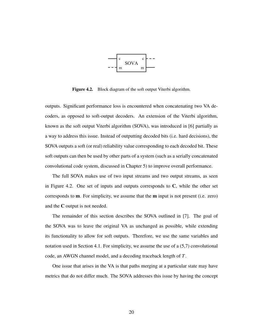
Figure 4.2. Block diagram of the soft output Viterbi algorithm.

outputs. Significant performance loss is encountered when concatenating two VA de-

coders, as opposed to soft-output decoders. An extension of the Viterbi algorithm,

known as the soft output Viterbi algorithm (SOVA), was introduced in [6] partially as

a way to address this issue. Instead of outputting decoded bits (i.e. hard decisions), the

SOVA outputs a soft (or real) reliability value corresponding to each decoded bit. These

soft outputs can then be used by other parts of a system (such as a serially concatenated

convolutional code system, discussed in Chapter 5) to improve overall performance.

The full SOVA makes use of two input streams and two output streams, as seen

in Figure 4.2. One set of inputs and outputs corresponds to C, while the other set

corresponds to m. For simplicity, we assume that the m input is not present (i.e. zero)

and the C output is not needed.

The remainder of this section describes the SOVA outlined in [7]. The goal of

the SOVA was to leave the original VA as unchanged as possible, while extending

its functionality to allow for soft outputs. Therefore, we use the same variables and

notation used in Section 4.1. For simplicity, we assume the use of a (5,7) convolutional

code, an AWGN channel model, and a decoding traceback length of T .

One issue that arises in the VA is that paths merging at a particular state may have

metrics that do not differ much. The SOVA addresses this issue by having the concept

20

of competing paths. We define a path metric candidate

M(i)K (q) = MK−1(qS(ei))+ γK(ei), (4.13)

where i ∈ {1,2}, qE(ei) = q, and γK(ei) is calculated according to Equation 4.6. There-

fore each state has two path metric candidates that are compared to select the updated

path metric

MK(q) = max{

M(1)K (q), M(2)

K (q)}, (4.14)

which ends up giving the same result as Equation 4.4. The value i = 1 is typically

assigned to the winning candidate, with i = 2 being assigned to the losing candidate.

Each time a path metric for state q is updated, the absolute difference between the

winning and losing candidates merging at state q is stored, or

∆K(q) =∣∣∣M(1)

K (q) − M(2)K (q)

∣∣∣ (4.15)

This provides information about the margin of victory enjoyed by the “best” path, which

is used to update other values within the SOVA.

In the same way as the VA, the SOVA can take advantage of a length T traceback

window. Instead of storing only the output decisions corresponding to the ML path, we

also consider output decisions for the 2ν − 1 other paths. This means we have a path

decision vector for each state q, or

mK(q) = {mK−T+1, · · · , mK} (4.16)

CK(q) = {cK−T+1, · · · , cK} . (4.17)

(The bold and capitalized C means that each element in the vector is also a vector.)

21

mK

(q) =(1)

ˆ

mK

(q) =(2)

ˆ

mK−1(qx) =

mK(q) =

{…,0,1,1}

{…,1,1,0}

{…,1,1}

mK−1(qy) = {…,0,1}

0

1

{…,0,1,1}

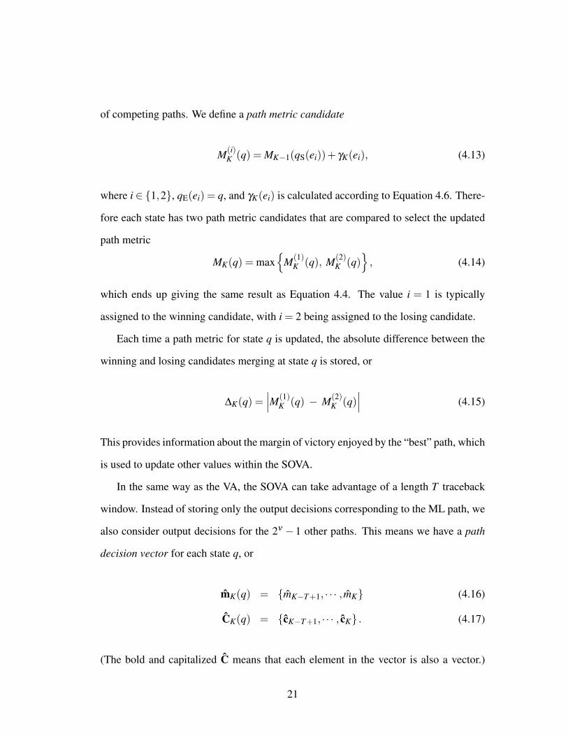
Figure 4.3. Illustration of merging path decision candidates.

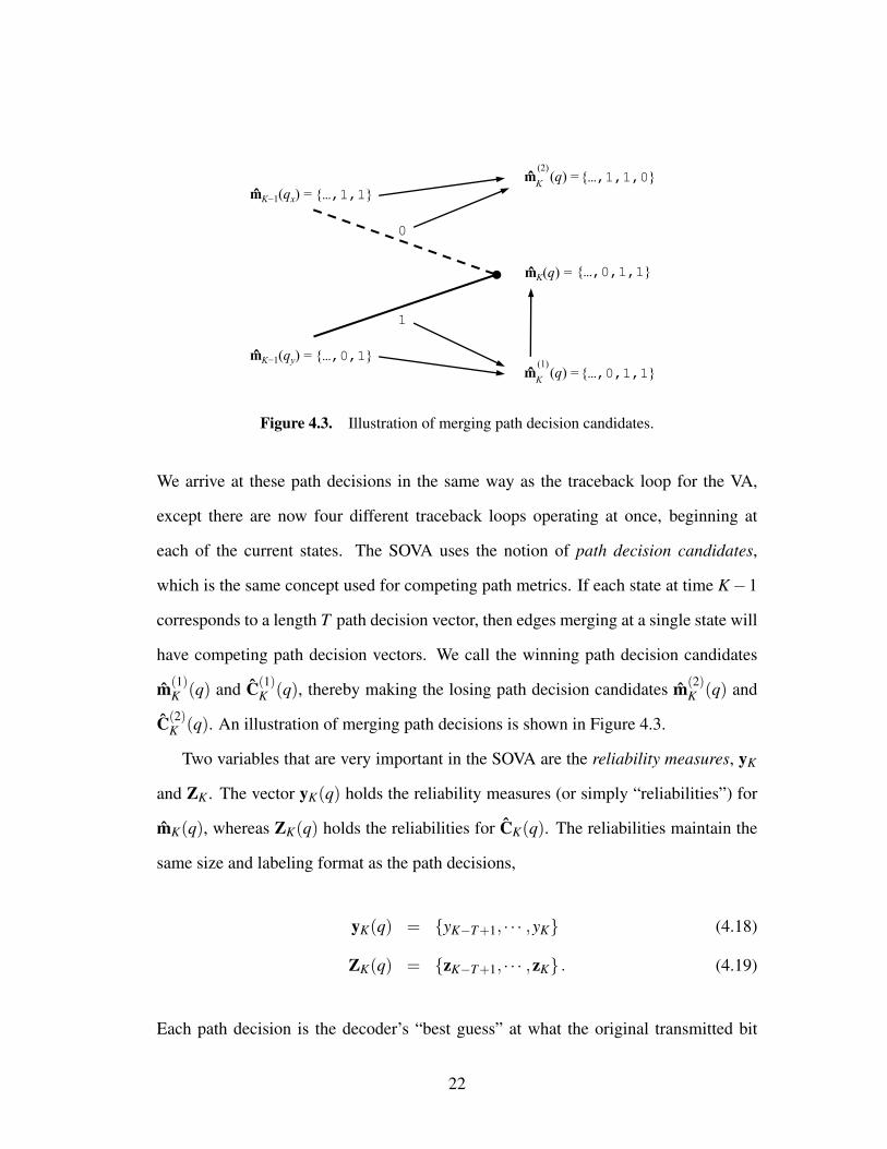
We arrive at these path decisions in the same way as the traceback loop for the VA,

except there are now four different traceback loops operating at once, beginning at

each of the current states. The SOVA uses the notion of path decision candidates,

which is the same concept used for competing path metrics. If each state at time K−1

corresponds to a length T path decision vector, then edges merging at a single state will

have competing path decision vectors. We call the winning path decision candidates

m(1)K (q) and C(1)

K (q), thereby making the losing path decision candidates m(2)K (q) and

C(2)K (q). An illustration of merging path decisions is shown in Figure 4.3.

Two variables that are very important in the SOVA are the reliability measures, yK

and ZK . The vector yK(q) holds the reliability measures (or simply “reliabilities”) for

mK(q), whereas ZK(q) holds the reliabilities for CK(q). The reliabilities maintain the

same size and labeling format as the path decisions,

yK(q) = {yK−T+1, · · · ,yK} (4.18)

ZK(q) = {zK−T+1, · · · ,zK} . (4.19)

Each path decision is the decoder’s “best guess” at what the original transmitted bit

22

was, and each reliability represents how confident we are that those path decisions

are correct. In the same way as the path decision candidates, we have the reliability

candidates y(1)K (q), y(2)K (q), Z(1)K (q), and Z(2)

K (q). The reliabilities are re-calculated for

every time step according to the path decision candidates and the current values of ∆.

We set the reliabilities at time K equal to ∆ for each state q, or

yK(q) = ∆K(q) (4.20)

zK(q) = {∆K(q),∆K(q)} (4.21)

This is because ∆ represents the reliability difference between the two most-likely code

sequences that terminate at state q. Next, we loop over the remaining reliabilities and

update them according to a comparison of the path decision candidates for each state

q. Each bit in path (1) is compared with the corresponding bit in path (2). This means

there are two cases for each comparison: equality and inequality. The update process

for yK(q) is as follows:

• Let J loop on the remaining reliabilities, or J ∈ {K−T +1, · · · ,K−1}.

• If m(1)J (q) 6= m(2)

J (q), then we update yJ(q) using the equation

yJ(q) = min{

∆K(q), y(1)J (q)}

(4.22)

• If m(1)J (q) = m(2)

J (q), then we update yJ(q) using the equation

yJ(q) = min{

∆K(q)+ y(2)J (q), y(1)J (q)}

(4.23)

We update ZK(q) in a similar fashion, however each element in ZK(q) is a vector of

23

two bits. Since we are comparing on a bit-by-bit basis, there will be two comparisons

for each element. Therefore the update process for ZK(q) is as follows:

• Let J be an outer loop index on the remaining reliabilities, or J ∈ {K − T +

1, · · · ,K− 1}. Let i be an inner loop index on the two values contained within

each element, or i ∈ {0,1}.

• If c(1)J (q)[i] 6= c(2)J (q)[i], then we update zJ(q)[i] using the equation

zJ(q)[i] = min{

∆K(q), z(1)J (q)[i]}

(4.24)

• If c(1)J (q)[i] = c(2)J (q)[i], then we update zJ(q)[i] using the equation

zJ(q)[i] = min{

∆K(q)+ z(2)J (q)[i], z(1)J (q)[i]}

(4.25)

The traceback loop of the SOVA is the same as that for the VA, with the addition of

reliability calculation. Before the reliabilities are output from the decoder, their signs

are changed according to the path decisions. In other words, each reliability becomes

negative if its corresponding path decision is a 0, and positive if the path decision is 1.

In addition, the input values are subtracted from the correspnding signed reliabilities.

This is due to the fact that what the decoder receives is extrinsic information, and must

be removed for the next round of processing.

24

Chapter 5

Serially Concatenated Convolutional

Codes

In the communication theory world, bit error rate (BER) performance is typically

improved by choosing longer and more complex codes. Unfortunately, they are not

always implementable in the hardware available today. Forney first introduced the idea

of concatenated codes in [8] as a way of dividing a long code into smaller, more man-

ageable pieces. His system consisted of inner and outer codes, with the outer usually

being longer and more complex than the inner. Typically, a convolutional code with

Viterbi decoding was concatenated with a Reed-Solomon code, with a resulting system

so powerful that NASA even adopted it as a standard for deep-space applications.

The idea of concatenating multiple convolutional codes was introduced in [9], and

was made possible in part by the the newly-developed soft output Viterbi algorithm

(SOVA). An inner SOVA decoder provides a 1–2 dB gain in BER performance over an

inner hard-decision Viterbi decoder [9]. The concatenation of convolutional codes was

then examined further in [10], in which the name "serially concatenated convolutional

code" (SCCC) came about.

25

An iterative decoding approach to SCCC’s was introduced in [11]. Instead of mak-

ing one pass over the concatenated decoders, the iterative method performs several. In-

formation from the outermost decoder is re-interleaved and fed back into the innermost

decoder. The iterative decoding method provides a significant increase in performance

over a single iteration, and in some cases approaches the theoretical limit.

Figures 5.1 and 5.2 show visualizations of the SCCC transmitter and receiver, re-

spectively. In the receiver, the updated probabilities from the inner decoder are de-

interleaved and provided as inputs to the outer decoder. Since there is never any up-

dated information about the m input to the outder decoder, it is assumed to be zero

(shown with a “ground” symbol). The updated probabilities of the outer decoder are

then re-interleaved and provided as additional information for the next pass in the it-

erative process. The use of interleavers (Π) helps the system manage bursts of errors,

which the Viterbi algorithm is very sensitive to.

Though several soft-input soft-output algorithms can be used for the inner and outer

decoders, we focus on the use of the SOVA for both. The hardware implementation

outlined in Chapter 6 provides the framework for a general purpose SOVA decoder that

can be used in multiple places in a SCCC system.

26

Outer

CC∏

Inner

CCm c m c

Map to

{−1,+1}sm

s AWGN r

Figure 5.1. A serially concatenated convolutional code transmitter.

Inner

Decoder∏−1

Outer

Decoder

∏

Map to

{0,1}

m

c

m

c

m

c

m

c

r

m

Figure 5.2. A serially concatenated convolutional code receiver with iter-ative decoding.

27

Chapter 6

Hardware Implementation

This chapter introduces a hardware implementation of the soft output Viterbi algo-

rithm (SOVA). The algorithm notations used throughout this chapter follow the same

format as found in Section 4.2.

6.1 Design

6.1.1 Code and Trellis

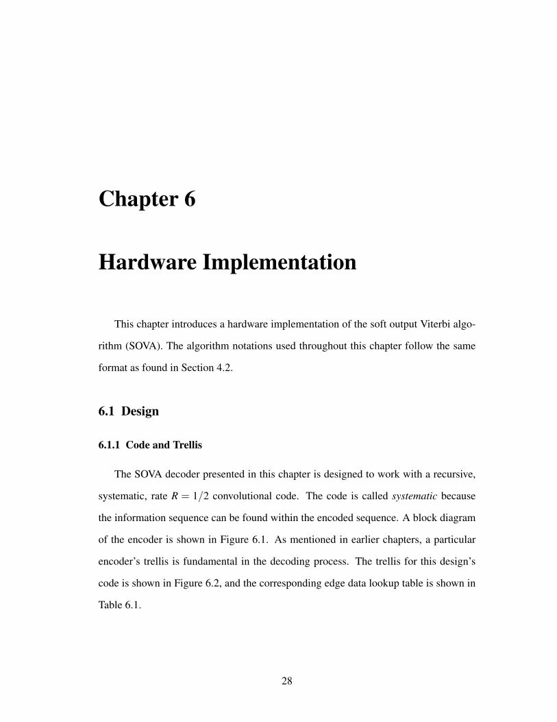
The SOVA decoder presented in this chapter is designed to work with a recursive,

systematic, rate R = 1/2 convolutional code. The code is called systematic because

the information sequence can be found within the encoded sequence. A block diagram

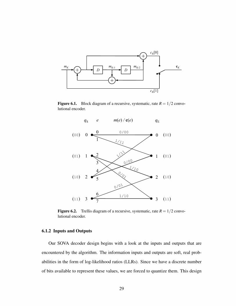
of the encoder is shown in Figure 6.1. As mentioned in earlier chapters, a particular

encoder’s trellis is fundamental in the decoding process. The trellis for this design’s

code is shown in Figure 6.2, and the corresponding edge data lookup table is shown in

Table 6.1.

28

D D

+

+

mK

mK-1 m

K-2

cK[0]

cK[1]

cK

+

Figure 6.1. Block diagram of a recursive, systematic, rate R = 1/2 convo-lutional encoder.

0/00

1/10

qS qE

0

2

3

1

0

2

3

1

e

0

1

2

3

4

5

6

7

m(e) / c(e)

(00)

(01)

(10)

(11)

(00)

(01)

(10)

(11)

Figure 6.2. Trellis diagram of a recursive, systematic, rate R = 1/2 convo-lutional encoder.

6.1.2 Inputs and Outputs

Our SOVA decoder design begins with a look at the inputs and outputs that are

encountered by the algorithm. The information inputs and outputs are soft, real prob-

abilities in the form of log-likelihood ratios (LLRs). Since we have a discrete number

of bits available to represent these values, we are forced to quantize them. This design

29

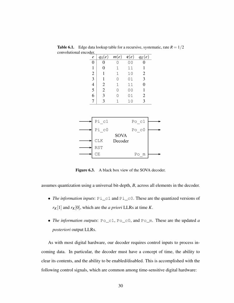
Table 6.1. Edge data lookup table for a recursive, systematic, rate R = 1/2convolutional encoder.

e qS(e) m(e) c(e) qE(e)0 0 0 00 01 0 1 11 12 1 1 10 23 1 0 01 34 2 1 11 05 2 0 00 16 3 0 01 27 3 1 10 3

CLK

RST

CE

Pi_c1

Pi_c0

SOVA

Decoder

Po_c1

Po_c0

Po_m

Figure 6.3. A black box view of the SOVA decoder.

assumes quantization using a universal bit-depth, B, across all elements in the decoder.

• The information inputs: Pi_c1 and Pi_c0. These are the quantized versions of

rK[1] and rK[0], which are the a priori LLRs at time K.

• The information outputs: Po_c1, Po_c0, and Po_m. These are the updated a

posteriori output LLRs.

As with most digital hardware, our decoder requires control inputs to process in-

coming data. In particular, the decoder must have a concept of time, the ability to

clear its contents, and the ability to be enabled/disabled. This is accomplished with the

following control signals, which are common among time-sensitive digital hardware:

30

Pi_c1

Pi_c0

CE

CLK

RST

Metric

Manager

(MM)

Hard-Decision

Traceback

Unit (HTU)

Reliability

Traceback

Unit (RTU)

Output

Calculator

(OC)Po_m

Po_c1

Po_c0

CTRL

Figure 6.4. The internal structure of the SOVA decoder.

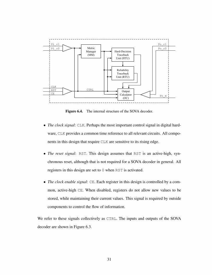
• The clock signal: CLK. Perhaps the most important control signal in digital hard-

ware, CLK provides a common time reference to all relevant circuits. All compo-

nents in this design that require CLK are sensitive to its rising edge.

• The reset signal: RST. This design assumes that RST is an active-high, syn-

chronous reset, although that is not required for a SOVA decoder in general. All

registers in this design are set to 0 when RST is activated.

• The clock enable signal: CE. Each register in this design is controlled by a com-

mon, active-high CE. When disabled, registers do not allow new values to be

stored, while maintaining their current values. This signal is required by outside

components to control the flow of information.

We refer to these signals collectively as CTRL. The inputs and outputs of the SOVA

decoder are shown in Figure 6.3.

31

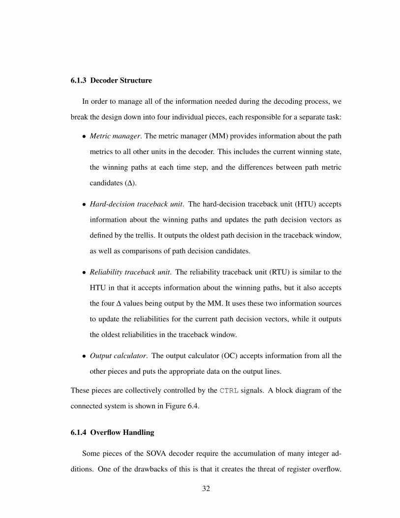
6.1.3 Decoder Structure

In order to manage all of the information needed during the decoding process, we

break the design down into four individual pieces, each responsible for a separate task:

• Metric manager. The metric manager (MM) provides information about the path

metrics to all other units in the decoder. This includes the current winning state,

the winning paths at each time step, and the differences between path metric

candidates (∆).

• Hard-decision traceback unit. The hard-decision traceback unit (HTU) accepts

information about the winning paths and updates the path decision vectors as

defined by the trellis. It outputs the oldest path decision in the traceback window,

as well as comparisons of path decision candidates.

• Reliability traceback unit. The reliability traceback unit (RTU) is similar to the

HTU in that it accepts information about the winning paths, but it also accepts

the four ∆ values being output by the MM. It uses these two information sources

to update the reliabilities for the current path decision vectors, while it outputs

the oldest reliabilities in the traceback window.

• Output calculator. The output calculator (OC) accepts information from all the

other pieces and puts the appropriate data on the output lines.

These pieces are collectively controlled by the CTRL signals. A block diagram of the

connected system is shown in Figure 6.4.

6.1.4 Overflow Handling

Some pieces of the SOVA decoder require the accumulation of many integer ad-

ditions. One of the drawbacks of this is that it creates the threat of register overflow.

32

max_val

+<

0

≥0

≥0

00

01

10

11

min_val

s1 s0

out

in0in1

Figure 6.5. An overflow-safe adding circuit.

Register overflow occurs when the combination of binary values results in a value out

of range. The resulting value “overflows,” either wrapping around from positive to

negative or negative to positive.

One way to handle overflow is to increase the bit widths of the addition operations.

This method is successful if the decoder is to be reset after a certain period of time,

but if the decoder runs long enough, it can still encounter overflow. We instead choose

to modify the additions to never wrap around in either direction. If two operands are

positive and their result is negative, then we set the result to be the maximum allowable

value. If two operands are negative and their result is positive, then we set the result to

be the minimum allowable value. The circuit for this overflow-safe adder is shown in

Figure 6.5.

This method of overflow handling is suboptimal, as we are restricting all integers to

fall into a certain range. Fortunately, the effect of removing this precision is negligible

for significant bit widths.

33

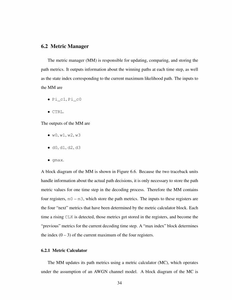
6.2 Metric Manager

The metric manager (MM) is responsible for updating, comparing, and storing the

path metrics. It outputs information about the winning paths at each time step, as well

as the state index corresponding to the current maximum likelihood path. The inputs to

the MM are

• Pi_c1, Pi_c0

• CTRL.

The outputs of the MM are

• w0, w1, w2, w3

• d0, d1, d2, d3

• gmax.

A block diagram of the MM is shown in Figure 6.6. Because the two traceback units

handle information about the actual path decisions, it is only necessary to store the path

metric values for one time step in the decoding process. Therefore the MM contains

four registers, m0 – m3, which store the path metrics. The inputs to these registers are

the four “next” metrics that have been determined by the metric calculator block. Each

time a rising CLK is detected, those metrics get stored in the registers, and become the

“previous” metrics for the current decoding time step. A “max index” block determines

the index (0 – 3) of the current maximum of the four registers.

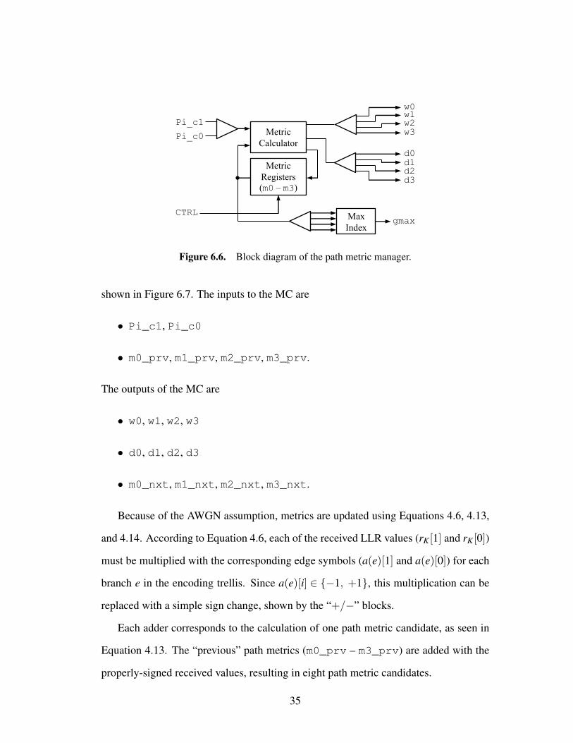
6.2.1 Metric Calculator

The MM updates its path metrics using a metric calculator (MC), which operates

under the assumption of an AWGN channel model. A block diagram of the MC is

34

Pi_c1

Pi_c0 Metric

Calculator

Metric

Registers

(m0 – m3)

CTRL

w0w1w2w3

d0d1d2d3

Max

Indexgmax

Figure 6.6. Block diagram of the path metric manager.

shown in Figure 6.7. The inputs to the MC are

• Pi_c1, Pi_c0

• m0_prv, m1_prv, m2_prv, m3_prv.

The outputs of the MC are

• w0, w1, w2, w3

• d0, d1, d2, d3

• m0_nxt, m1_nxt, m2_nxt, m3_nxt.

Because of the AWGN assumption, metrics are updated using Equations 4.6, 4.13,

and 4.14. According to Equation 4.6, each of the received LLR values (rK[1] and rK[0])

must be multiplied with the corresponding edge symbols (a(e)[1] and a(e)[0]) for each

branch e in the encoding trellis. Since a(e)[i] ∈ {−1, +1}, this multiplication can be

replaced with a simple sign change, shown by the “+/−” blocks.

Each adder corresponds to the calculation of one path metric candidate, as seen in

Equation 4.13. The “previous” path metrics (m0_prv – m3_prv) are added with the

properly-signed received values, resulting in eight path metric candidates.

35

m0_prv

m2_prv

m0_prv

m2_prv

m1_prv

m3_prv

m1_prv

m3_prv

adder≤

Δadder

adder

adder

adder

adder

adder

adder

≤

Δ

≤

Δ

≤

Δ

m0_nxt

m1_nxt

m2_nxt

m3_nxt

w0

d0

w1

d1

w2

d2

w3

d3

Pi_c1Pi_c0

+/−

+/−

m0_prv

m1_prv

m2_prv

m3_prv

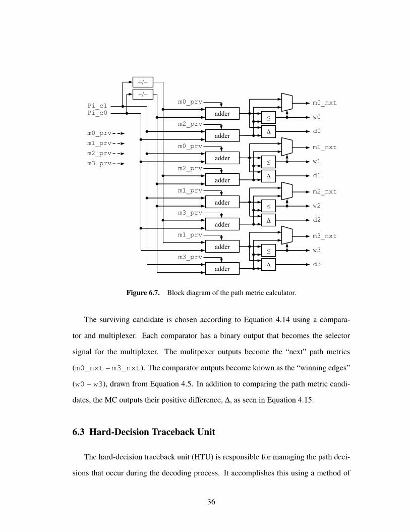
Figure 6.7. Block diagram of the path metric calculator.

The surviving candidate is chosen according to Equation 4.14 using a compara-

tor and multiplexer. Each comparator has a binary output that becomes the selector

signal for the multiplexer. The mulitpexer outputs become the “next” path metrics

(m0_nxt – m3_nxt). The comparator outputs become known as the “winning edges”

(w0 – w3), drawn from Equation 4.5. In addition to comparing the path metric candi-

dates, the MC outputs their positive difference, ∆, as seen in Equation 4.15.

6.3 Hard-Decision Traceback Unit

The hard-decision traceback unit (HTU) is responsible for managing the path deci-

sions that occur during the decoding process. It accomplishes this using a method of

36

reg1

reg0

0

1

reg1(T − 1 downto 1)1

decision

value

winning branch

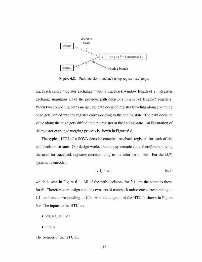
Figure 6.8. Path decision traceback using register exchange.

traceback called “register exchange,” with a traceback window length of T . Register

exchange maintains all of the previous path decisions in a set of length-T registers.

When two competing paths merge, the path decision register traveling along a winning

edge gets copied into the register corresponding to the ending state. The path decision

value along the edge gets shifted into the register at the ending state. An illustration of

the register exchange merging process is shown in Figure 6.8.

The typical HTU of a SOVA decoder contains traceback registers for each of the

path decision streams. Our design works around a systematic code, therefore removing

the need for traceback registers corresponding to the information bits. For the (5,7)

systematic encoder,

c[1] = m, (6.1)

which is seen in Figure 6.1. All of the path decisions for c[1] are the same as those

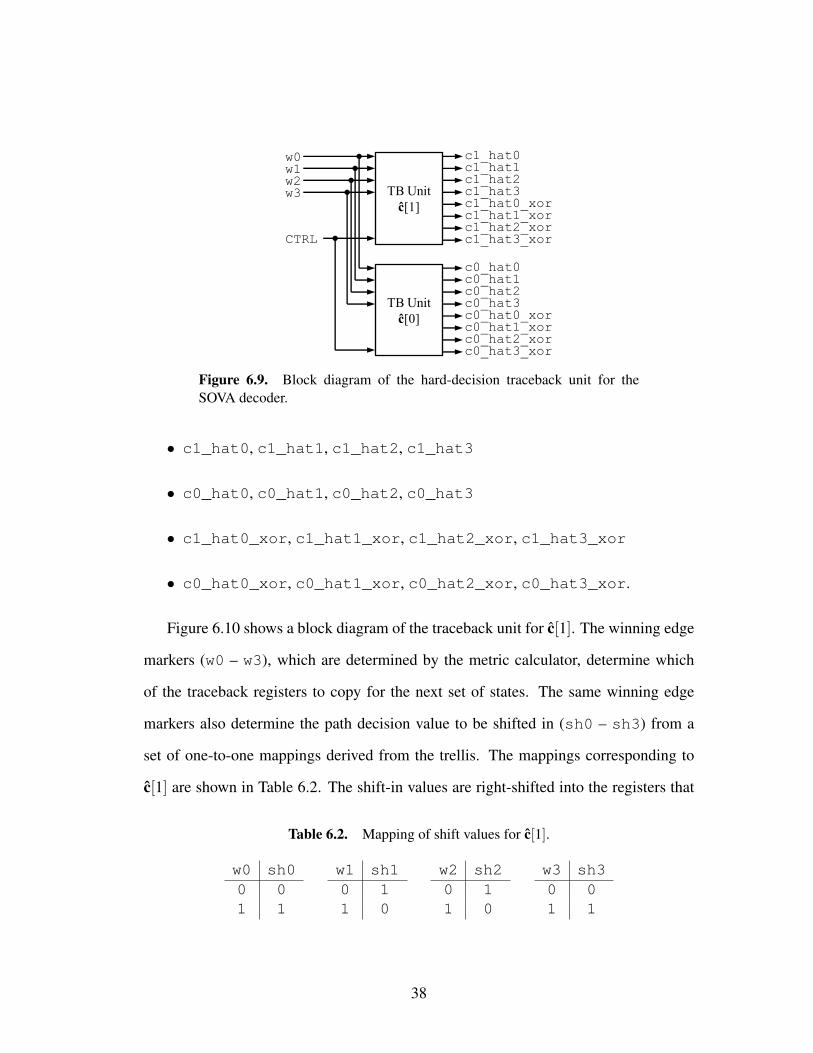
for m. Therefore our design contains two sets of traceback units: one corresponding to

c[1], and one corresponding to c[0]. A block diagram of the HTU is shown in Figure

6.9. The inputs to the HTU are

• w0, w1, w2, w3

• CTRL.

The outputs of the HTU are

37

w0w1w2w3

CTRL

TB Unit

ĉ[1]

c1_hat0c1_hat1c1_hat2c1_hat3c1_hat0_xorc1_hat1_xorc1_hat2_xorc1_hat3_xor

TB Unit

ĉ[0]

c0_hat0c0_hat1c0_hat2c0_hat3c0_hat0_xorc0_hat1_xorc0_hat2_xorc0_hat3_xor

Figure 6.9. Block diagram of the hard-decision traceback unit for theSOVA decoder.

• c1_hat0, c1_hat1, c1_hat2, c1_hat3

• c0_hat0, c0_hat1, c0_hat2, c0_hat3

• c1_hat0_xor, c1_hat1_xor, c1_hat2_xor, c1_hat3_xor

• c0_hat0_xor, c0_hat1_xor, c0_hat2_xor, c0_hat3_xor.

Figure 6.10 shows a block diagram of the traceback unit for c[1]. The winning edge

markers (w0 – w3), which are determined by the metric calculator, determine which

of the traceback registers to copy for the next set of states. The same winning edge

markers also determine the path decision value to be shifted in (sh0 – sh3) from a

set of one-to-one mappings derived from the trellis. The mappings corresponding to

c[1] are shown in Table 6.2. The shift-in values are right-shifted into the registers that

Table 6.2. Mapping of shift values for c[1].

w0 sh00 01 1

w1 sh10 11 0

w2 sh20 11 0

w3 sh30 01 1

38

Right

Shift

reg0

reg1

reg2

reg3

w0w1w2w3

CTRL

tb0

tb1

tb2

tb3

w0

w1

w2

w3

Right

Shift

Right

Shift

Right

Shift

Shift

Values

c[1](e)

sh0sh1sh2sh3

sh0

sh1

sh2

sh3

tb0

tb1

tb2

tb3

xor

xor

c1_hat0_xor

c1_hat1_xor

c1_hat2_xor

c1_hat3_xor

c1_hat0tb0[0]

c1_hat1tb1[0]

c1_hat2tb2[0]

c1_hat3tb3[0]

Figure 6.10. Block diagram of the traceback unit corresponding to c[1].

were selected by the winning edge markers. The results becomes the next states of the

traceback registers, and the oldest bit of each register goes to the output.

In addition to outputting the oldest path decisions, each TB unit outputs four vec-

tors of comparison bits, one for each set of merging path decision candidates. This is

necessary to update the reliabilities, as each path decision candidate is compared with

its competitor to choose Equation 4.24 or 4.25. Since the path decision candidates in

our traceback units are just bits, we can simply use the xor operation to determine if

they are equal or not equal. If they are equal, the value of the xor will be 0. If they are

not equal, the value of the xor will be 1.

6.4 Reliability Traceback Unit

The reliability traceback unit (RTU) is responsible for storing and updating the

reliabilities of the path decisions. The RTU uses the same traceback window length as

39

the HTU, although instead of maintaining four length-T registers, the RTU keeps track

of four length-T arrays of length-B registers. In other words, there are four arrays, each

with T locations. Each location in an array contains a register with B bits.

Since the HTU only keeps track of path decisions c[1] and c[0], the RTU only main-

tains the reliabilities z[1] and z[0]. The inputs to the RTU are:

• w0, w1, w2, w3

• d0, d1, d2, d3

• c1_hat0_xor, c1_hat1_xor, c1_hat2_xor, c1_hat3_xor

• c0_hat0_xor, c0_hat1_xor, c0_hat2_xor, c0_hat3_xor

• CTRL.

The outputs of the RTU are

• z1_0, z1_1, z1_2, z1_3

• z0_0, z0_1, z0_2, z0_3.

Figure 6.11 shows a block diagram of the RTU. It is made up of two individual

traceback units corresponding to z[1] and z[0]. Each unit outputs the oldest reliability

value from each traceback array.

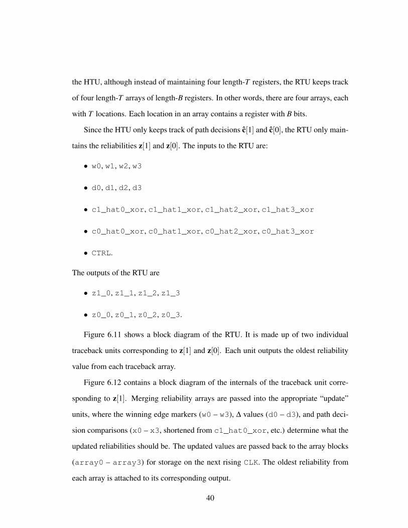
Figure 6.12 contains a block diagram of the internals of the traceback unit corre-

sponding to z[1]. Merging reliability arrays are passed into the appropriate “update”

units, where the winning edge markers (w0 – w3), ∆ values (d0 – d3), and path deci-

sion comparisons (x0 – x3, shortened from c1_hat0_xor, etc.) determine what the

updated reliabilities should be. The updated values are passed back to the array blocks

(array0 – array3) for storage on the next rising CLK. The oldest reliability from

each array is attached to its corresponding output.

40

w0w1w2w3

CTRL

TB Unit

z[1]

z1_0z1_1z1_2z1_3

c1_hat0_xorc1_hat1_xorc1_hat2_xorc1_hat3_xor

c0_hat0_xorc0_hat1_xorc0_hat2_xorc0_hat3_xor

z0_0z0_1z0_2z0_3

d0d1d2d3

TB Unit

z[0]

Figure 6.11. Block diagram of the reliability traceback unit for the SOVAdecoder.

6.5 Output Calculator

The output calculator (OC) is responsible for determining the final outputs of the

decoder, based on information received from all other units. The inputs to the OC are:

• z1_0, z1_1, z1_2, z1_3

• z0_0, z0_1, z0_2, z0_3

• c1_hat0, c1_hat1, c1_hat2, c1_hat3

• c0_hat0, c0_hat1, c0_hat2, c0_hat3

• Pi_c1, Pi_c0

• gmax

41

array0

array1

array2

array3

w0w1w2w3

CTRL

tb0

tb1

tb2

tb3

d0d1d2d3

c1_hat0_xorc1_hat1_xorc1_hat2_xorc1_hat3_xor

x0x1x2x3

w0

Update

d0

tb0

z1_0tb0[0]

x0

w1

Update

d1

tb1

z1_1tb1[0]

x1

w2

Update

d2

tb2

z1_2tb2[0]

x2

w3

Update

d3

tb3

z1_3tb3[0]

x3

Figure 6.12. Block diagram of the traceback unit corresponding to z[1].

• CTRL.

The outputs of the OC are

• z1_0, z1_1, z1_2, z1_3

• z0_0, z0_1, z0_2, z0_3.

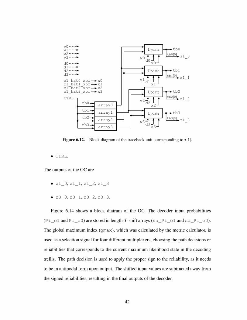
Figure 6.14 shows a block diatram of the OC. The decoder input probabilities

(Pi_c1 and Pi_c0) are stored in length-T shift arrays (sa_Pi_c1 and sa_Pi_c0).

The global maximum index (gmax), which was calculated by the metric calculator, is

used as a selection signal for four different multiplexers, choosing the path decisions or

reliabilities that corresponds to the current maximum likelihood state in the decoding

trellis. The path decision is used to apply the proper sign to the reliability, as it needs

to be in antipodal form upon output. The shifted input values are subtracted away from

the signed reliabilities, resulting in the final outputs of the decoder.

42

dxw

d

x

min

w

z_in0[0]

z_in1[0] min

adderd

z_out[0]0

1

0

1

w

1

0

d

x

min

w

z_in0[1]

z_in1[1] min

adderd

z_out[1]0

1

0

1

w

1

0

. . .d

x

min

w

z_in0[T−2]

z_in1[T−2] min

adderd

z_out[T−2]0

1

0

1

w

1

0

z_out[T−1]d

Figure 6.13. Block diagram of a reliability update unit.

Pi_c0

gmax

00

01

11

10

z1_0z1_1z1_2z1_3

gmax

00

01

11

10

c1_hat0c1_hat1c1_hat2c1_hat3

+ / − 0

1

Po_c1

Po_m

Po_c0

z1_0z1_1z1_2z1_3c1_hat0c1_hat1c1_hat2c1_hat3

z0_0z0_1z0_2z0_3c0_hat0c0_hat1c0_hat2c0_hat3

Pi_c1

CTRLgmax

sa_Pi_c1Pi_c1

CTRL

sa_Pi_c0Pi_c0

CTRL

subtract

subtract

z1

z0

gmax

00

01

11

10

z0_0z0_1z0_2z0_3

gmax

00

01

11

10

c0_hat0c0_hat1c0_hat2c0_hat3

+ / − 0

1

z1

z0

Figure 6.14. Block diagram of the output calculator.

43

Chapter 7

Performance Results

This chapter gives performance results of the VHDL implementation of the SOVA

decoder design outlined in Chapter 6. The VHDL version of the decoder was compared

with a given reference decoder written in MATLAB, which was known to be accurate.

Throughout this chapter we refer to them as the “VHDL decoder” and “MATLAB

decoder,” respectively.

7.1 Comparison with Software Reference

The VHDL and MATLAB decoders were compared by simulating over various bit

widths and traceback lengths. MATLAB was used to generate noisy, encoded streams

of data, and each decoder used a common traceback length of T . The VHDL decoder

was run in the ModelSim simulator, and its inputs were quantized with the bit width, B.

A bit error rate (BER) comparison was done using only the information bit decisions

(i.e. m or c[1]), meaning the reliability outputs of each decoder were mapped to 0’s and

1’s before being compared for equality. Simulations were done using four bit widths

and two traceback window lengths, with B ∈ {6, 7, 8, 9} and T ∈ {8, 16}.

44

Each simulation was run over a minimum of 1,000,000 transmitted bits, with a

requirement of at least 100 bit errors after decoding. While these values are on the low

end of what can be used to generate an “accurate” BER plot, they are sufficient for

determining whether the VHDL decoder is operating correctly or not.

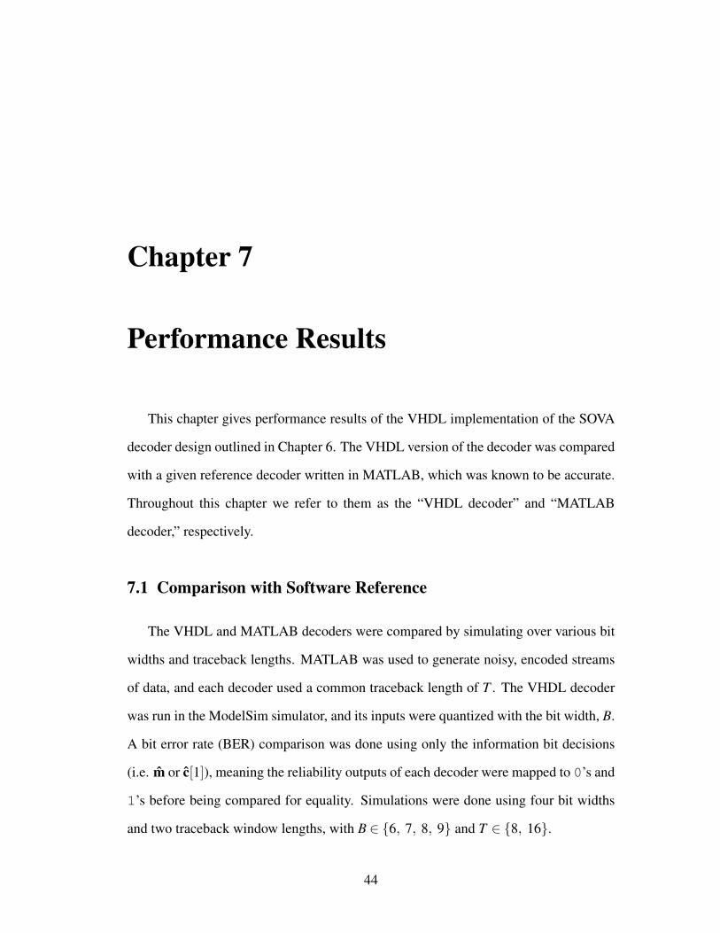
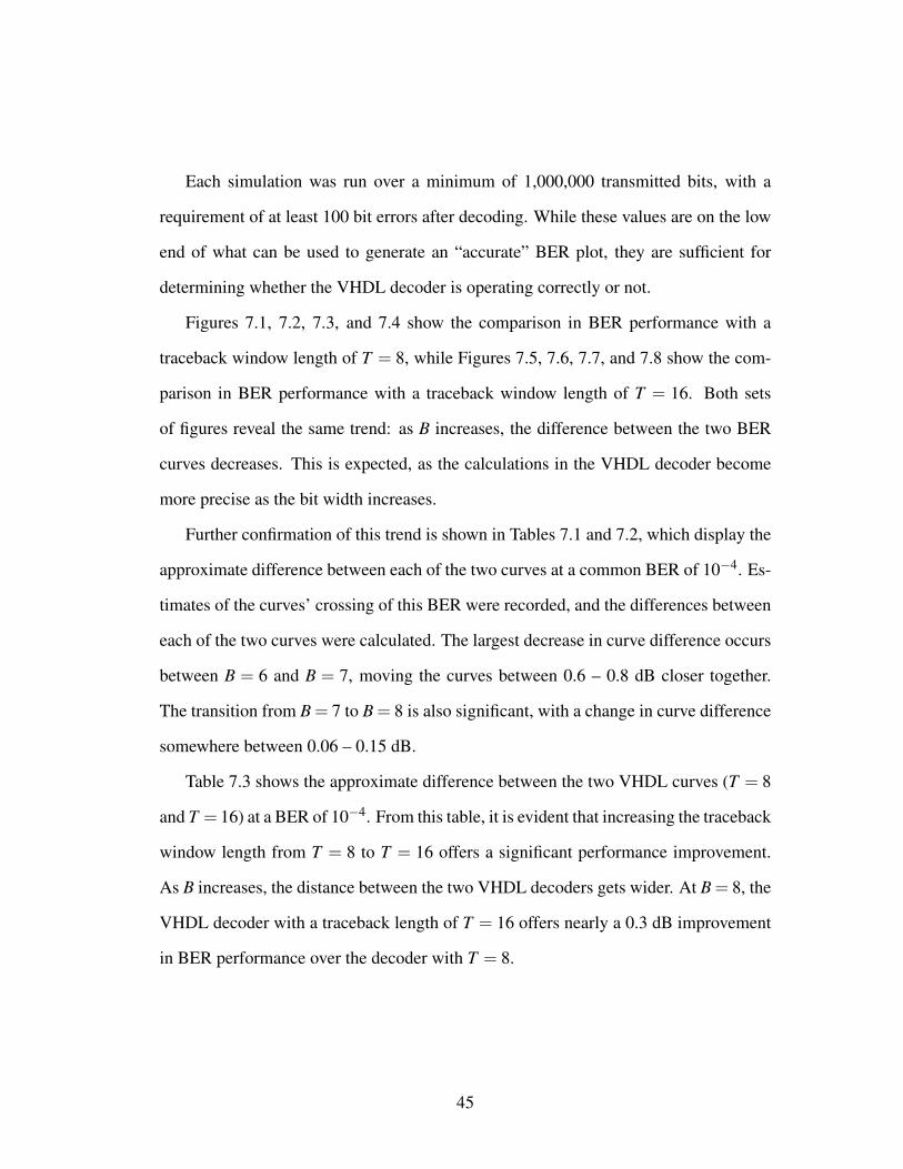
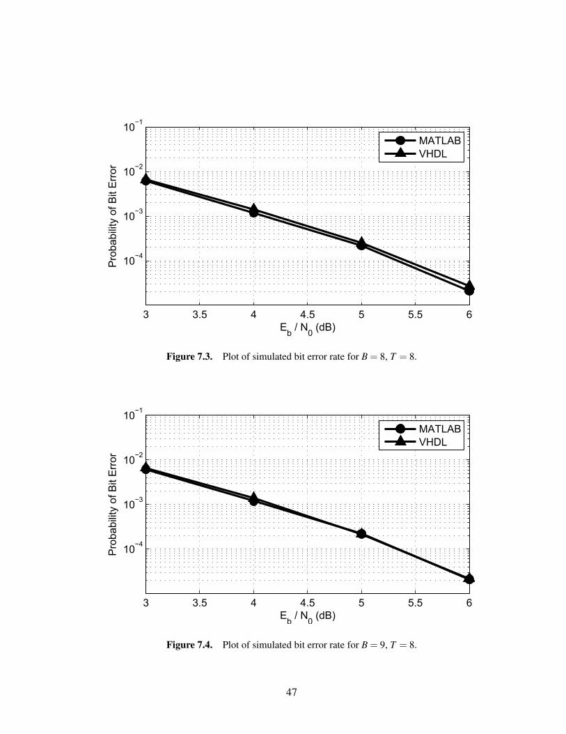
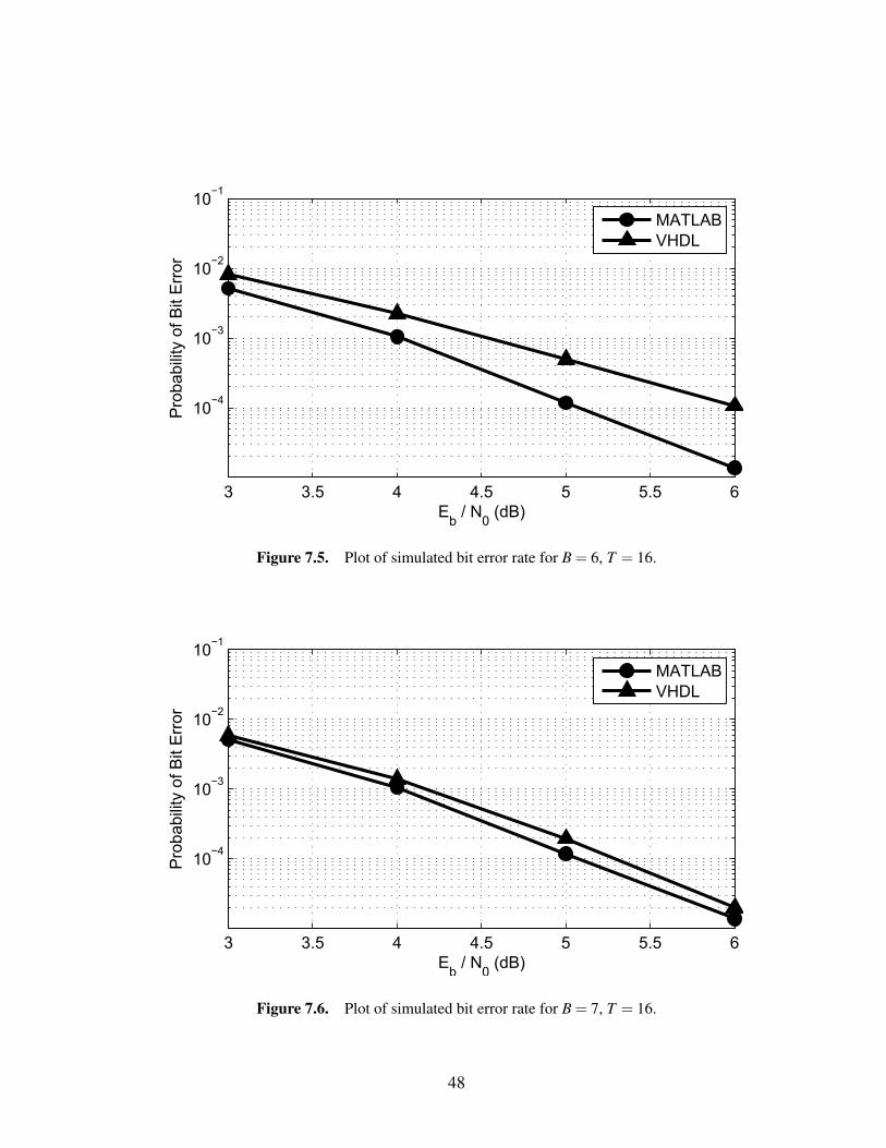
Figures 7.1, 7.2, 7.3, and 7.4 show the comparison in BER performance with a

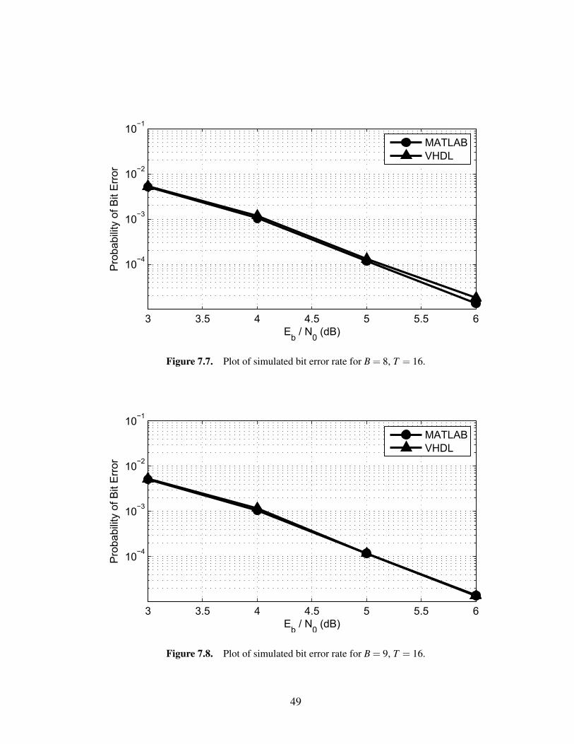
traceback window length of T = 8, while Figures 7.5, 7.6, 7.7, and 7.8 show the com-

parison in BER performance with a traceback window length of T = 16. Both sets

of figures reveal the same trend: as B increases, the difference between the two BER

curves decreases. This is expected, as the calculations in the VHDL decoder become

more precise as the bit width increases.

Further confirmation of this trend is shown in Tables 7.1 and 7.2, which display the

approximate difference between each of the two curves at a common BER of 10−4. Es-

timates of the curves’ crossing of this BER were recorded, and the differences between

each of the two curves were calculated. The largest decrease in curve difference occurs

between B = 6 and B = 7, moving the curves between 0.6 – 0.8 dB closer together.

The transition from B = 7 to B = 8 is also significant, with a change in curve difference

somewhere between 0.06 – 0.15 dB.

Table 7.3 shows the approximate difference between the two VHDL curves (T = 8

and T = 16) at a BER of 10−4. From this table, it is evident that increasing the traceback

window length from T = 8 to T = 16 offers a significant performance improvement.

As B increases, the distance between the two VHDL decoders gets wider. At B = 8, the

VHDL decoder with a traceback length of T = 16 offers nearly a 0.3 dB improvement

in BER performance over the decoder with T = 8.

45

3 3.5 4 4.5 5 5.5 6

10−4

10−3

10−2

10−1

Eb

/ N0

(dB)

Pro

ba

bili

ty o

f B

it E

rror

MATLAB

VHDL

Figure 7.1. Plot of simulated bit error rate for B = 6, T = 8.

3 3.5 4 4.5 5 5.5 6

10−4

10−3

10−2

10−1

Eb

/ N0

(dB)

Pro

ba

bili

ty o

f B

it E

rror

MATLAB

VHDL

Figure 7.2. Plot of simulated bit error rate for B = 7, T = 8.

46

3 3.5 4 4.5 5 5.5 6

10−4

10−3

10−2

10−1

Eb

/ N0

(dB)

Pro

ba

bili

ty o

f B

it E

rror

MATLAB

VHDL

Figure 7.3. Plot of simulated bit error rate for B = 8, T = 8.

3 3.5 4 4.5 5 5.5 6

10−4

10−3

10−2

10−1

Eb

/ N0

(dB)

Pro

ba

bili

ty o

f B

it E

rror

MATLAB

VHDL

Figure 7.4. Plot of simulated bit error rate for B = 9, T = 8.

47

3 3.5 4 4.5 5 5.5 6

10−4

10−3

10−2

10−1

Eb

/ N0

(dB)

Pro

ba

bili

ty o

f B

it E

rror

MATLAB

VHDL

Figure 7.5. Plot of simulated bit error rate for B = 6, T = 16.

3 3.5 4 4.5 5 5.5 6

10−4

10−3

10−2

10−1

Eb

/ N0

(dB)

Pro

ba

bili

ty o

f B

it E

rror

MATLAB

VHDL

Figure 7.6. Plot of simulated bit error rate for B = 7, T = 16.

48

3 3.5 4 4.5 5 5.5 6

10−4

10−3

10−2

10−1

Eb

/ N0

(dB)

Pro

ba

bili

ty o

f B

it E

rror

MATLAB

VHDL

Figure 7.7. Plot of simulated bit error rate for B = 8, T = 16.

3 3.5 4 4.5 5 5.5 6

10−4

10−3

10−2

10−1

Eb

/ N0

(dB)

Pro

ba

bili

ty o

f B

it E

rror

MATLAB

VHDL

Figure 7.8. Plot of simulated bit error rate for B = 9, T = 16.

49

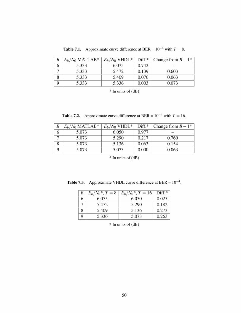
Table 7.1. Approximate curve difference at BER = 10−4 with T = 8.

B Eb/N0 MATLAB* Eb/N0 VHDL* Diff.* Change from B−1*6 5.333 6.075 0.742 –7 5.333 5.472 0.139 0.6038 5.333 5.409 0.076 0.0639 5.333 5.336 0.003 0.073

* In units of (dB)

Table 7.2. Approximate curve difference at BER = 10−4 with T = 16.

B Eb/N0 MATLAB* Eb/N0 VHDL* Diff.* Change from B−1*6 5.073 6.050 0.977 –7 5.073 5.290 0.217 0.7608 5.073 5.136 0.063 0.1549 5.073 5.073 0.000 0.063

* In units of (dB)

Table 7.3. Approximate VHDL curve difference at BER = 10−4.

B Eb/N0*, T = 8 Eb/N0*, T = 16 Diff.*6 6.075 6.050 0.0257 5.472 5.290 0.1828 5.409 5.136 0.2739 5.336 5.073 0.263

* In units of (dB)

50

7.2 Hardware Performance

The VHDL used to define the SOVA decoder was synthesized, mapped, and routed

for use on the XC5VLX110T FPGA, which is a member of Xilinx’s Virtex-5 family.

The processing was done using the Xilinx ISE design tools. A user constraint was

defined for the clock signal to have a period of 7ns with a 50% duty cycle. This forced

ISE to work harder in its attempts to find the maximum clock frequency, although

in some cases the constraint could not be met. As in the BER simulations, designs

were built using the traceback window lengths T ∈ {8, 16} and the bit widths B ∈

{6, 7, 8, 9}.

Tables 7.4 and 7.5 show the hardware results obtained in the building of the designs.

According to [12], the XC5VLX110T has 17,280 available Virtex-5 slices, with each

slice containing four lookup tables (LUTs) and four flip-flops (FFs). We see in each

table that the overall footprint of the SOVA decoder is relatively small, with all builds

using under 12% of the available slices. As expected, a larger bit width generally

yields a larger slice utilization, however this is not true when going from B = 8 to

B = 9 for T = 16. This can be attributed to the non-deterministic nature of the Xilinx

ISE processes. In other words, multiple builds of the same design can sometimes yield

different results. Therefore rebuilding the designs for B = 8 and B = 9 may result in

different slice utilizations and clock frequencies.

The more interesting result of the builds is the difference in maximum clock fre-

quencies. The odd-numbered bit widths appear to result in lower clock frequencies

than do the even-numbered bit widths. This can be explained in part by the makeup of

the Virtex-5 slices. Each slice contains four LUTs and FFs, and therefore can be used

more efficiently in designs with an even bit width. The maximum clock frequencies for

B = 6 and B = 8 are within 0.2% of each other for both traceback lengths, suggesting

51

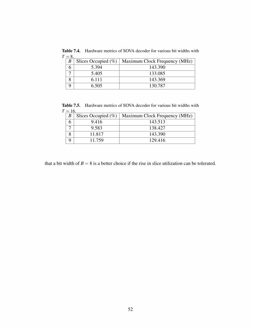
Table 7.4. Hardware metrics of SOVA decoder for various bit widths withT = 8.

B Slices Occupied (%) Maximum Clock Frequency (MHz)6 5.394 143.3907 5.405 133.0858 6.111 143.3699 6.505 130.787

Table 7.5. Hardware metrics of SOVA decoder for various bit widths withT = 16.

B Slices Occupied (%) Maximum Clock Frequency (MHz)6 9.416 143.5137 9.583 138.4278 11.817 143.3909 11.759 129.416

that a bit width of B = 8 is a better choice if the rise in slice utilization can be tolerated.

52

Chapter 8

Conclusion

8.1 Interpretation of Results

The results of the simulations in Chapter 7 indicate that the VHDL decoder success-

fully performs the soft output Viterbi algorithm. For each of the bit widths tested, the

difference between each pair of BER curves was less than 1.0 dB, with the commonly-

used bit width B = 8 yielding a curve difference of less than 0.08 dB. One must also

keep in mind that the BER curves in Chapter 7 correspond to only one iteration through

a SOVA decoder. In the final SCCC system, there may be as many as ten decoding

iterations, with information passing through two separate SOVA decoders per iteration.

The data also suggest that for each B> 8, the increase in BER performance becomes

smaller and smaller, until it aligns with the software reference decoder. Since B = 8 is

a very common bit width, it becomes a clear choice for use in most applications. It can

be assumed, however, that increasing the bit width to B = 16 will provide even more

accuracy, while at the same time following the standards of most hardware systems.

The comparison of results for different traceback lengths reveals that performance

is gained as the traceback length increases. This is an expected result, as performance

53

should increase with the traceback length, until a point is reached in which the per-

formance gain is insignificant. It is up to the designer to decide which value of T

yields BER performance that is “good enough,” however this value can also be deter-

mined through simulation. Increasing the traceback length also significantly increases

the amount of space used on an FPGA, so careful consideration must be taken when

choosing this value.

8.2 Suggested Improvements

The decoder design approach presented in this thesis is very much software-based.

In other words, focus was first placed on the simplicity of the VHDL code, rather

than potential optimizations provided by the hardware. Work can be done to improve

upon the speed and size of the structures contained in the design. One example is

the current method of overflow prevention. It may be possible to remove this in the

adder/subtractor circuits, while calculating the bit widths necessary to widen their in-

puts and outputs to accomodate all possible values. Such a change may allow for a

decrease in the error encountered by restricting the range of all integers that go through

an adder/subtractor, while providing a small boost in clock speed.

In its current state, the design is very much centered around a particular shape of

trellis. Though the information contained on each edge can quickly be changed, the

shape and size of the trellis are fixed. One major improvement would be the inclusion

of circuitry to make a general-purpose SOVA decoder that can operate on any type of

trellis. Such an improvement would provide the ability to change the structure of the

convolutional code without having to change the circuit.

54

References

[1] T. K. Moon, Error Correction Coding: Mathematical Methods and Algorithms.

Wiley, 2005.

[2] J. G. Proakis and M. Salehi, Digital Communications. McGraw-Hill, 2008.

[3] A. Viterbi, “Error Bounds for Convolutional Codes and an Asymptotically Opti-

mum Decoding Algorithm,” IEEE Transactions on Information Theory, vol. 13,

pp. 260 – 269, April 1967.

[4] G. D. Forney, Jr., “The Viterbi Algorithm,” Proceedings of the IEEE, vol. 61,

pp. 268 – 278, March 1973.

[5] F. Hemmati and D. Costello, Jr., “Truncation Error Probability in Viterbi Decod-

ing,” IEEE Transactions on Communications, vol. 25, pp. 530 – 532, May 1977.

[6] J. Hagenauer and P. Hoeher, “A Viterbi Algorithm with Soft-Decision Outputs

and its Applications,” in Global Telecommunications Conference, 1989, and Ex-

hibition. Communications Technology for the 1990s and Beyond. GLOBECOM

’89., IEEE, vol. 3, pp. 1680 – 1686, November 1989.

[7] M. P. C. Fossorier, F. Burkert, S. Lin, and J. Hagenauer, “On the Equivalence

Between SOVA and Max-Log-MAP Decodings,” IEEE Communications Letters,

vol. 2, pp. 137–139, May 1998.

55

[8] G. D. Forney, Concatenated Codes. Cambridge: M.I.T. Press, 1966.

[9] J. Hagenauer and P. Hoeher, “Concatenated Vitebi Decoding,” in Proceedings of

the International Workshop on Information Theory, 1989.

[10] S. Benedetto and G. Montorsi, “Serial concatenation of block and convolutional

codes,” Electronics Letters, vol. 32, pp. 887 – 888, September 1996.

[11] S. Benedetto and G. Montorsi, “Iterative decoding of serially concatenated con-

volutional codes,” Electronics Letters, vol. 32, pp. 1186 – 1188, June 1996.

[12] Xilinx, “Virtex-5 Family Overview: Product Specification,” February 2009.

DS100 (v5.0).

56