A Hardware Implementation of the Soft Output Viterbi Algorithm

A Hardware Implementation of the Soft Output Viterbi Algorithm for Serially Concatenated Convolutional Codes

Brett WerlingM.S. StudentInformation & Telecommunication Technology CenterThe University of Kansas

• Introduction• Background• Decoding Convolutional Codes• Hardware Implementation• Performance Results• Conclusions and Future Work

2

OverviewOverview

3

IntroductionIntroduction

• High-Rate High-Speed Forward Error Correction Architectures for Aeronautical Telemetry (HFEC)

»ITTC – University of Kansas»2-year project»Sponsored by the Test Resource Management Center

(TRMC) T&E/S&T Program»FEC decoder prototypes

•SOQPSK-TG modulation»LDPC»SCCC

•Other modulations

HFEC ProjectHFEC Project

4

• There is a need for a convolutional code SOVA decoder block written in a hardware description language

»Used multiple places within the HFEC decoder prototypes»VHDL code can be modified to fit various convolutional codes

with relative ease• Future students must be able to use the implementation for

the SCCC decoder integration»Black box

MotivationMotivation

5

• Convolutional Codes• Channel Models• Serially Concatenated Convolutional Codes

BackgroundBackground

6

• Class of linear forward error correction (FEC) codes• Use convolution to encode data sequences

»Encoders are usually binary digital filters»Coding rate R = k / n

•k input symbols•n output symbols

• Structure allows for much flexibility»Convolutional codes operate on streams of data

•Linear block codes assume fixed-length messages»Lower encoding and decoding complexity than linear block

codes for same coding rates

7

Convolutional CodesConvolutional Codes

• Convolutional encoders are binary digital filters»FIR filters are called feedforward encoders»IIR filters are called feedback encoders


8

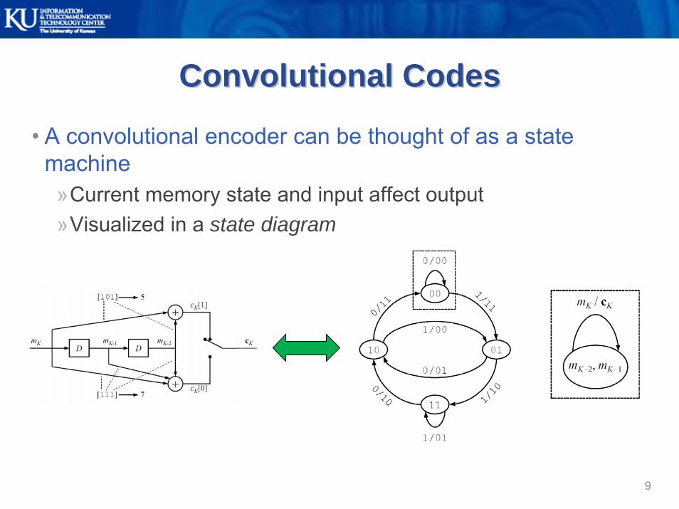
• A convolutional encoder can be thought of as a state machine

»Current memory state and input affect output»Visualized in a state diagram


9

• Another representation is the trellis diagram»State diagram shown over time»Heavily used in many decoding algorithms

•Viterbi algorithm•Soft output Viterbi algorithm•Others


10

K K + 1


• Each stage in the trellis corresponds to one unit of time

• Useful labels»State index: q

•Starting state: qS

•Ending state: qE

»Edge index: e»Input / output:

m(e) / c(e)

11

• All of the information in a trellis diagram can be contained in a simple lookup table

»Each edge index corresponds to one row in the table


12



13

• Communication links are affected by their environment»Thermal noise»Signal reflections»Similar communication links

• Two common channel models are used when evaluating the performance of a convolutional code

»Binary symmetric channel (BSC)»Additive white Gaussian noise channel (AWGN)

Channel ModelsChannel Models

14

Channel Models Channel Models -- BSCBSC

• Binary symmetric channel (BSC)»Bit is transmitted either correctly

or incorrectly (binary)•Error occurs with probability p•Success occurs with probability 1 − p

»Transmission modeled as a binary addition

•XOR operation

15

r = s n+

Channel Models Channel Models -- AWGNAWGN

• Additive white Gaussian noise channel (AWGN)»Bits are modulated before

transmission (e.g. BPSK)• s contains values in {−1, +1}

»Noise values are soft (real)•Gaussian random variables

»Transmission modeled as an addition of reals

16

r = s + n



17

• SCCC Encoder»Two differing convolutional codes are serially concatenated

before transmission•Separated by an interleaver•Most previous concatenation schemes involved a convolutional code and a Reed Solomon code

Serially Concatenated Convolutional CodesSerially Concatenated Convolutional Codes

18

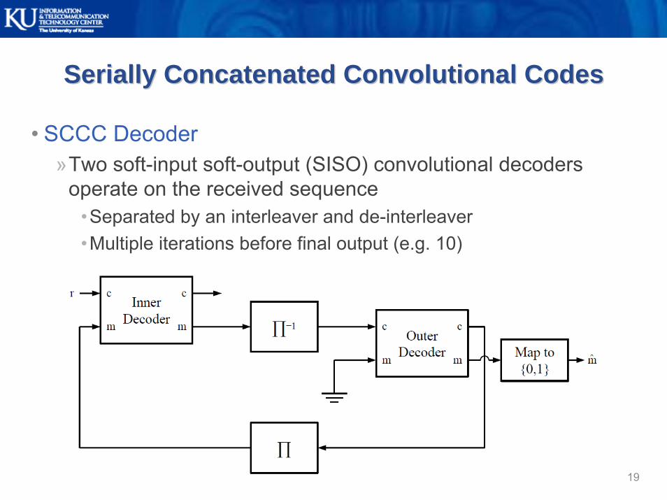
• SCCC Decoder»Two soft-input soft-output (SISO) convolutional decoders

operate on the received sequence•Separated by an interleaver and de-interleaver•Multiple iterations before final output (e.g. 10)


19

• SCCC Decoder»Two soft-input soft-output (SISO) convolutional decoders

operate on the received sequence•Separated by an interleaver and de-interleaver•Multiple iterations before final output (e.g. 10)


20

21

Decoding Convolutional CodesDecoding Convolutional Codes

• Most common algorithm for decoding a convolutionally-encoded sequence

• Uses maximum likelihood sequence estimation to decode a noisy sequence

»Uses trellis structure to compare possible encoding paths»Keeps track of only the paths that occur with maximum

likelihood• Needs only two* passes over a received sequence to

determine output»BCJR and Max-Log MAP algorithms need three»*Can use a windowing technique in the second pass

Viterbi AlgorithmViterbi Algorithm

22

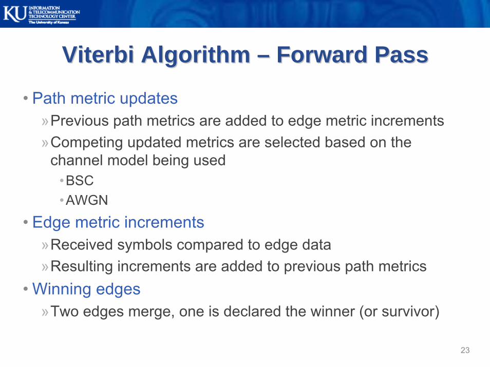
• Path metric updates»Previous path metrics are added to edge metric increments»Competing updated metrics are selected based on the

channel model being used•BSC•AWGN

• Edge metric increments»Received symbols compared to edge data»Resulting increments are added to previous path metrics

• Winning edges»Two edges merge, one is declared the winner (or survivor)

Viterbi Algorithm Viterbi Algorithm –– Forward PassForward Pass

23

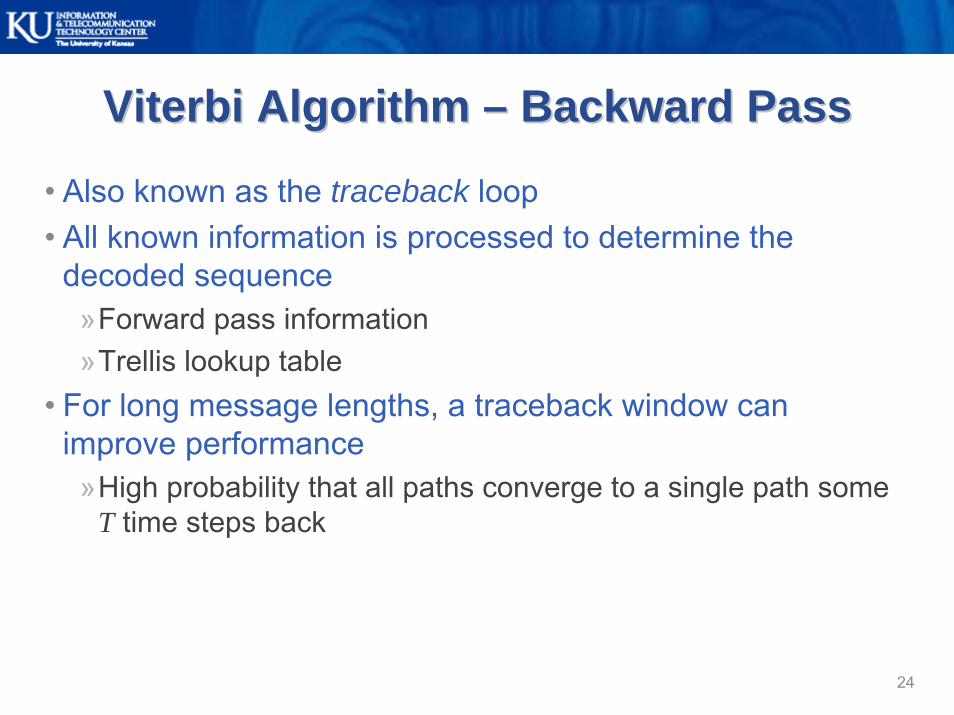
• Also known as the traceback loop• All known information is processed to determine the

decoded sequence»Forward pass information»Trellis lookup table

• For long message lengths, a traceback window can improve performance

»High probability that all paths converge to a single path some T time steps back

Viterbi Algorithm Viterbi Algorithm –– Backward PassBackward Pass

24

• Extension of the Viterbi algorithm• Addition of soft outputs allows it to be more useful in an

SCCC system»Significant performance gain over use of Viterbi algorithm in

an SCCC decoder

Soft Output Viterbi AlgorithmSoft Output Viterbi Algorithm

25

• Same basic calculations as the Viterbi algorithm• Additional calculations

»Competing path differences»Path decision reliabilities»Subtraction of prior probabilities

• Same traceback window applies to the traceback loop»Includes additional reliability output calculation

Soft Output Viterbi AlgorithmSoft Output Viterbi Algorithm

26

• Begin with an empty trellis and like-valued path metrics

Soft Output Viterbi Algorithm Soft Output Viterbi Algorithm –– ExampleExample

27

00

01

10

11

00

01

10

11

00

01

10

11

r0 = {-1, -1}0

0

0

0

• Calculate the edge metric increments for the current trellis stage (in this case AWGN calculations)


28

00

01

10

11

00

01

10

11

00

01

10

11

r0 = {-1, -1}0

0

0

0

1-1

0

0-1

1

0

0

• Add the edge metric increments to their corresponding path metrics


29

00

01

10

11

00

01

10

11

00

01

10

11

r0 = {-1, -1}0

0

0

0

1-1

0

0-1

1

0

0

1-1

-1

1

0

0

0

0

• Find the absolute difference between competing edges• Choose the winning metric as the new path metric


30

00

01

10

11

00

01

10

11

00

01

10

11

r0 = {-1, -1}0

0

0

0

1-1

0

0-1

1

0

0

1-1

-1

1

0

0

0

0

1

1

0

0

Δ0(0) = 2

Δ0(1) = 2

Δ0(2) = 0

Δ0(3) = 0

• Mark the winning edges


31

00

01

10

11

00

01

10

11

00

01

10

11

r0 = {-1, -1}0

0

0

0

1-1

0

0-1

1

0

0

1-1

-1

1

0

0

0

0

1

1

0

0

Δ0(0) = 2

Δ0(1) = 2

Δ0(2) = 0

Δ0(3) = 0

• The trellis after two time steps


32

00

01

10

11

00

01

10

11

00

01

10

11

r0 = {-1, -1}0

0

0

0

1-1

0

0-1

1

0

0

1-1

-1

1

0

0

0

0

1

1

0

0

Δ0(0) = 2

Δ0(1) = 2

Δ0(2) = 0

Δ0(3) = 0

1

2

1

1

-11

0

01

-1

0

0

01

2

-1

1

0

1

0

Δ1(0) = 1

Δ1(1) = 3

Δ1(2) = 1

Δ1(3) = 1

r1 = {1, 1}

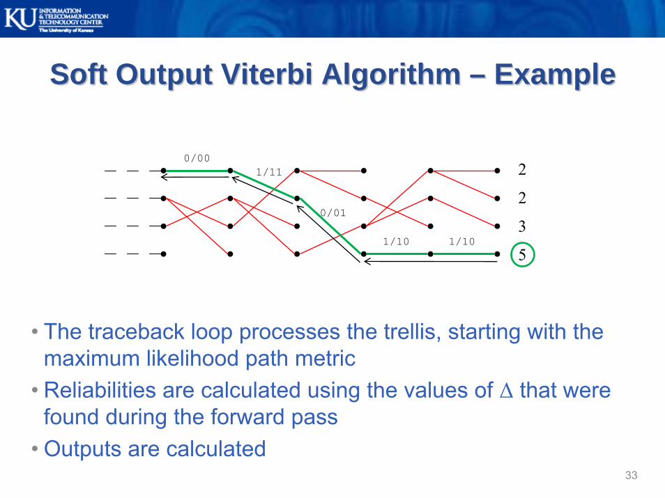
• The traceback loop processes the trellis, starting with the maximum likelihood path metric

• Reliabilities are calculated using the values of Δ that were found during the forward pass

• Outputs are calculated


33

2

2

3

51/101/10

0/01

1/110/00

34

Hardware ImplementationHardware Implementation

• Designed to work with a systematic rate R = ½ code»Systematic – message sequence appears within the encoded

sequence• Design decisions

»Traceback is done with register exchange»Overflow is prevented by clipping values at a maximum and

minimum»Path metrics are periodically reduced to prevent them from

becoming too large»Two global design variables

•Bit width: B•Traceback length: T


35

• Divided into four blocks»Metric Manager (MM)»Hard Decision Traceback Unit (HTU)»Reliability Traceback Unit (RTU)»Output Calculator (OC)


36

• Metric Manager»Handles storage and calculation of path metrics»Determines winning edges»Finds absolute path metric differences


37

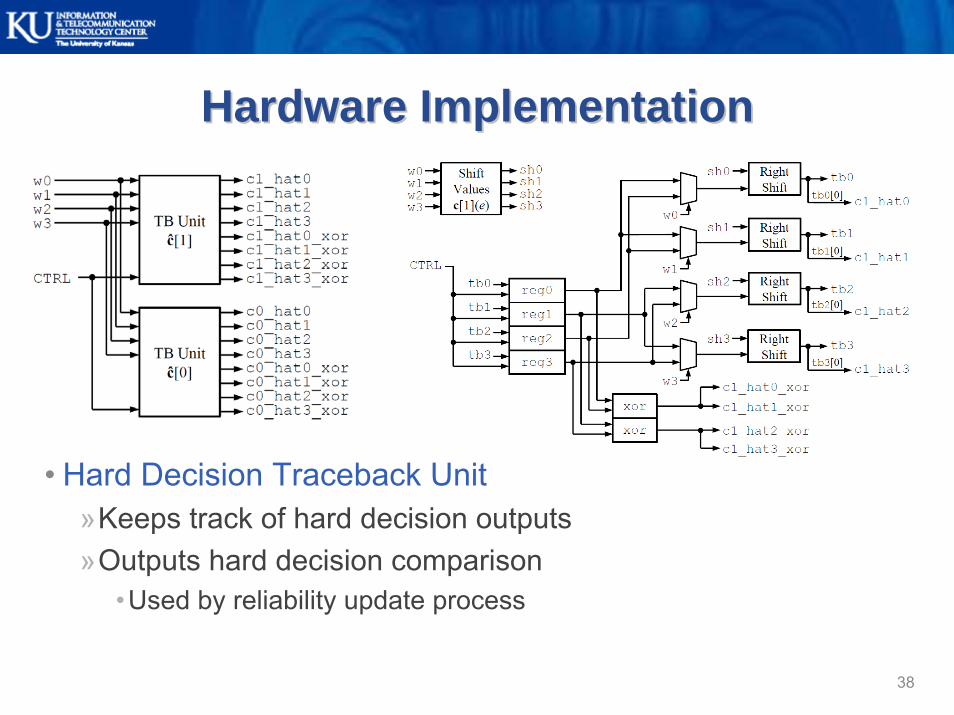
• Hard Decision Traceback Unit»Keeps track of hard decision outputs»Outputs hard decision comparison

•Used by reliability update process


38

• Reliability Traceback Unit»Keeps track of reliabilities»Updates each reliability for every clock cycle


39

• Output Calculator»Determines final output of the decoder


40

41

Performance ResultsPerformance Results

• The VHDL decoder was compared with a reference decoder written in Matlab

»Matlab version known to be correct• Simulations run for varying SNRs and traceback lengths

»Noise values generated in Matlab»VHDL decoder simulated in ModelSim using Matlab data

• Simulation requirements»Transmitted information bits ≥ 1,000,000»Information bit errors ≥ 100

Performance Results Performance Results –– Software ComparisonSoftware Comparison

42

• Traceback length T = 8


43

B = 6

B = 8

B = 7

B = 9

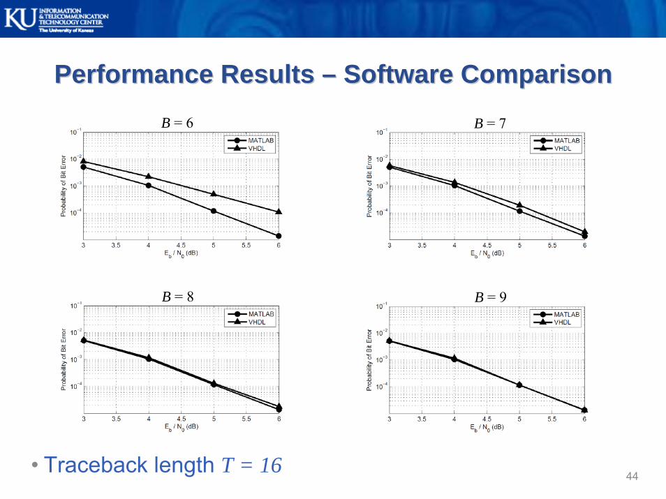
• Traceback length T = 16


44

B = 6 B = 7

B = 8 B = 9

• VHDL implementation approaches Matlab implementation as B increases

»Expected result – higher precision• Increase in BER performance as traceback length

increases»Also expected – designer must determine which traceback

length provides “good enough” performance


45

• VHDL synthesized using Xilinx ISE for the XC5VLX110T FPGA

»All builds use < 12% of the slices available»Maximum clock speeds are fast enough to be used in the

SCCC decoder

Performance Results Performance Results –– HardwareHardware

46

T = 8

T = 16

47

Conclusions and Future WorkConclusions and Future Work

• The hardware implementation successfully performs the soft output Viterbi algorithm

• For all bit widths tested, VHDL curve differs from Matlab curve by < 1 dB

»For B = 8, difference is < 0.08 dB• Performance increases as traceback length increases

»Tradeoff between hardware size and decoder precision• Post-synthesis results

»Small – all designs < 12% slice utilization»Fast – clock speeds all > 129 MHz

Summary of ResultsSummary of Results

48

• New method of overflow prevention»Current design “clips” values, restricting them to fall within a

certain range»Work can be done to maintain precision

• FPGA optimization»Current design approach is very much software-based»Future designs can take advantage of FPGA features

•Size and speed can be further improved

• Generalized trellis»Current design focuses on a particular trellis»Trellis-defining inputs could offer more flexibility

Future WorkFuture Work

49

50

Questions?Questions?

A Hardware Implementation of the Soft Output Viterbi Algorithm

Documents

Transcript of A Hardware Implementation of the Soft Output Viterbi Algorithm