A Handbook of Statistical Analyses Using R.pdf
207
A Handbook of Statistical Analyses Using R Brian S. Everitt and Torsten Hothorn
-
Upload
nguyenthuan -
Category
Documents
-
view
249 -
download
3
Transcript of A Handbook of Statistical Analyses Using R.pdf

A Handbook of Statistical AnalysesUsing R
Brian S. Everitt and Torsten Hothorn

Preface
This book is intended as a guide to data analysis with the R system for sta-tistical computing. R is an environment incorporating an implementation ofthe S programming language, which is powerful, flexible and has excellentgraphical facilities (R Development Core Team, 2005). In the Handbook weaim to give relatively brief and straightforward descriptions of how to conducta range of statistical analyses using R. Each chapter deals with the analysisappropriate for one or several data sets. A brief account of the relevant statisti-cal background is included in each chapter along with appropriate references,but our prime focus is on how to use R and how to interpret results. Wehope the book will provide students and researchers in many disciplines witha self-contained means of using R to analyse their data. R is an open-sourceproject developed by dozens of volunteers for more than ten years now and isavailable from the Internet under the General Public Licence. R has becomethe lingua franca of statistical computing. Increasingly, implementations ofnew statistical methodology first appear as R add-on packages. In some com-munities, such as in bioinformatics, R already is the primary workhorse forstatistical analyses. Because the sources of the R system are open and avail-able to everyone without restrictions and because of its powerful language andgraphical capabilities, R has started to become the main computing engine forreproducible statistical research (Leisch, 2002a,b, 2003, Leisch and Rossini,2003, Gentleman, 2005). For a reproducible piece of research, the originalobservations, all data preprocessing steps, the statistical analysis as well asthe scientific report form a unity and all need to be available for inspection,reproduction and modification by the readers. Reproducibility is a natural re-quirement for textbooks such as the ‘Handbook of Statistical Analyses UsingR’ and therefore this book is fully reproducible using an R version greater orequal to 2.4.0. All analyses and results, including figures and tables, can bereproduced by the reader without having to retype a single line of R code. Thedata sets presented in this book are collected in a dedicated add-on packagecalled HSAUR accompanying this book. The package can be installed fromthe Comprehensive R Archive Network (CRAN) via
R> install.packages("HSAUR")
and its functionality is attached by
R> library("HSAUR")
The relevant parts of each chapter are available as a vignette, basically adocument including both the R sources and the rendered output of every

analysis contained in the book. For example, the first chapter can be inspectedbyR> vignette("Ch_introduction_to_R", package = "HSAUR")
and the R sources are available for reproducing our analyses byR> edit(vignette("Ch_introduction_to_R", package = "HSAUR"))
An overview on all chapter vignettes included in the package can be obtainedfromR> vignette(package = "HSAUR")
We welcome comments on the R package HSAUR, and where we think theseadd to or improve our analysis of a data set we will incorporate them intothe package and, hopefully at a later stage, into a revised or second editionof the book. Plots and tables of results obtained from R are all labelled as‘Figures’ in the text. For the graphical material, the corresponding figure alsocontains the ‘essence’ of the R code used to produce the figure, although thiscode may differ a little from that given in the HSAUR package, since the lat-ter may include some features, for example thicker line widths, designed tomake a basic plot more suitable for publication. We would like to thank the RDevelopment Core Team for the R system, and authors of contributed add-onpackages, particularly Uwe Ligges and Vince Carey for helpful advice on scat-terplot3d and gee. Kurt Hornik, Ludwig A. Hothorn, Fritz Leisch and RafaelWeißbach provided good advice with some statistical and technical problems.We are also very grateful to Achim Zeileis for reading the entire manuscript,pointing out inconsistencies or even bugs and for making many suggestionswhich have led to improvements. Lastly we would like to thank the CRC Pressstaff, in particular Rob Calver, for their support during the preparation of thebook. Any errors in the book are, of course, the joint responsibility of the twoauthors.
Brian S. Everitt and Torsten HothornLondon and Erlangen, December 2005

Bibliography
Gentleman, R. (2005), “Reproducible research: A bioinformatics case study,”Statistical Applications in Genetics and Molecular Biology , 4, URL http://www.bepress.com/sagmb/vol4/iss1/art2, article 2.
Leisch, F. (2002a), “Sweave: Dynamic generation of statistical reports usingliterate data analysis,” in Compstat 2002 — Proceedings in ComputationalStatistics, eds. W. Hardle and B. Ronz, Physica Verlag, Heidelberg, pp.575–580, ISBN 3-7908-1517-9.
Leisch, F. (2002b), “Sweave, Part I: Mixing R and LATEX,” R News, 2, 28–31,URL http://CRAN.R-project.org/doc/Rnews/.
Leisch, F. (2003), “Sweave, Part II: Package vignettes,” R News, 3, 21–24,URL http://CRAN.R-project.org/doc/Rnews/.
Leisch, F. and Rossini, A. J. (2003), “Reproducible statistical research,”Chance, 16, 46–50.
R Development Core Team (2005), R: A Language and Environment for Sta-tistical Computing , R Foundation for Statistical Computing, Vienna, Aus-tria, URL http://www.R-project.org, ISBN 3-900051-07-0.

CHAPTER 1
An Introduction to R
1.1 What Is R?
The R system for statistical computing is an environment for data analysis andgraphics. The root of R is the S language, developed by John Chambers andcolleagues (Becker et al., 1988, Chambers and Hastie, 1992, Chambers, 1998)at Bell Laboratories (formerly AT&T, now owned by Lucent Technologies)starting in the 1960s. The S language was designed and developed as a pro-gramming language for data analysis tasks but in fact it is a full-featured pro-gramming language in its current implementations. The development of the Rsystem for statistical computing is heavily influenced by the open source idea:The base distribution of R and a large number of user contributed extensionsare available under the terms of the Free Software Foundation’s GNU GeneralPublic License in source code form. This licence has two major implicationsfor the data analyst working with R. The complete source code is availableand thus the practitioner can investigate the details of the implementation ofa special method, can make changes and can distribute modifications to col-leagues. As a side-effect, the R system for statistical computing is available toeveryone. All scientists, especially including those working in developing coun-tries, have access to state-of-the-art tools for statistical data analysis withoutadditional costs. With the help of the R system for statistical computing, re-search really becomes reproducible when both the data and the results of alldata analysis steps reported in a paper are available to the readers throughan R transcript file. R is most widely used for teaching undergraduate andgraduate statistics classes at universities all over the world because studentscan freely use the statistical computing tools. The base distribution of R ismaintained by a small group of statisticians, the R Development Core Team.A huge amount of additional functionality is implemented in add-on packagesauthored and maintained by a large group of volunteers. The main source ofinformation about the R system is the world wide web with the official homepage of the R project being
http://www.R-project.org
All resources are available from this page: the R system itself, a collectionof add-on packages, manuals, documentation and more. The intention of thischapter is to give a rather informal introduction to basic concepts and datamanipulation techniques for the R novice. Instead of a rigid treatment ofthe technical background, the most common tasks are illustrated by practical
1

2 AN INTRODUCTION TO R
examples and it is our hope that this will enable readers to get started withouttoo many problems.
1.2 Installing R
The R system for statistical computing consists of two major parts: the basesystem and a collection of user contributed add-on packages. The R language isimplemented in the base system. Implementations of statistical and graphicalprocedures are separated from the base system and are organised in the formof packages. A package is a collection of functions, examples and documen-tation. The functionality of a package is often focused on a special statisticalmethodology. Both the base system and packages are distributed via the Com-prehensive R Archive Network (CRAN) accessible under
http://CRAN.R-project.org
1.2.1 The Base System and the First Steps
The base system is available in source form and in precompiled form for variousUnix systems, Windows platforms and Mac OS X. For the data analyst, itis sufficient to download the precompiled binary distribution and install itlocally. Windows users follow the link
http://CRAN.R-project.org/bin/windows/base/release.htm
download the corresponding file (currently named rw2040.exe), execute itlocally and follow the instructions given by the installer.
Depending on the operating system, R can be started eitherby typing ‘R’ on the shell (Unix systems) or by clicking on theR symbol (as shown left) created by the installer (Windows).R comes without any frills and on start up shows simply ashort introductory message including the version number anda prompt ‘>’:
R : Copyright 2006 The R Foundation for Statistical ComputingVersion 2.4.0 (2006-10-03), ISBN 3-900051-07-0
R is free software and comes with ABSOLUTELY NO WARRANTY.You are welcome to redistribute it under certain conditions.Type 'license()' or 'licence()' for distribution details.
R is a collaborative project with many contributors.Type 'contributors()' for more information and'citation()' on how to cite R or R packages in publications.
Type 'demo()' for some demos, 'help()' for on-line help, or'help.start()' for an HTML browser interface to help.Type 'q()' to quit R.
>

INSTALLING R 3
One can change the appearance of the prompt by> options(prompt = "R> ")
and we will use the prompt R> for the display of the code examples through-out this book. Essentially, the R system evaluates commands typed on the Rprompt and returns the results of the computations. The end of a commandis indicated by the return key. Virtually all introductory texts on R start withan example using R as pocket calculator, and so do we:R> x <- sqrt(25) + 2
This simple statement asks the R interpreter to calculate√
25 and then to add2. The result of the operation is assigned to an R object with variable name x.The assignment operator <- binds the value of its right hand side to a variablename on the left hand side. The value of the object x can be inspected simplyby typingR> x
[1] 7
which, implicitly, calls the print method:R> print(x)
[1] 7
1.2.2 Packages
The base distribution already comes with some high-priority add-on packages,namely
KernSmooth MASS boot classcluster foreign lattice mgcvnlme nnet rpart spatialsurvival base datasets grDevicesgraphics grid methods splinesstats stats4 tcltk toolsutils
The packages listed here implement standard statistical functionality, for ex-ample linear models, classical tests, a huge collection of high-level plottingfunctions or tools for survival analysis; many of these will be described andused in later chapters. Packages not included in the base distribution can be in-stalled directly from the R prompt. At the time of writing this chapter, 858 usercontributed packages covering almost all fields of statistical methodology wereavailable. Given that an Internet connection is available, a package is installedby supplying the name of the package to the function install.packages. If,for example, add-on functionality for robust estimation of covariance matricesvia sandwich estimators is required (for example in Chapter 11), the sandwichpackage (Zeileis, 2004) can be downloaded and installed viaR> install.packages("sandwich")

4 AN INTRODUCTION TO R
The package functionality is available after attaching the package by
R> library("sandwich")
A comprehensive list of available packages can be obtained from
http://CRAN.R-project.org/src/contrib/PACKAGES.html
Note that on Windows operating systems, precompiled versions of packagesare downloaded and installed. In contrast, packages are compiled locally beforethey are installed on Unix systems.
1.3 Help and Documentation
Roughly, three different forms of documentation for the R system for statis-tical computing may be distinguished: online help that comes with the basedistribution or packages, electronic manuals and publications work in the formof books etc. The help system is a collection of manual pages describing eachuser-visible function and data set that comes with R. A manual page is shownin a pager or web browser when the name of the function we would like to gethelp for is supplied to the help function
R> help("mean")
or, for short,
R> ?mean
Each manual page consists of a general description, the argument list of thedocumented function with a description of each single argument, informationabout the return value of the function and, optionally, references, cross-linksand, in most cases, executable examples. The function help.search is helpfulfor searching within manual pages. An overview on documented topics in anadd-on package is given, for example for the sandwich package, by
R> help(package = "sandwich")
Often a package comes along with an additional document describing the pack-age functionality and giving examples. Such a document is called a vignette(Leisch, 2003, Gentleman, 2005). The sandwich package vignette is openedusing
R> vignette("sandwich")
More extensive documentation is available electronically from the collectionof manuals at
http://CRAN.R-project.org/manuals.html
For the beginner, at least the first and the second document of the followingfour manuals (R Development Core Team, 2005a,b,c,d) are mandatory:
An Introduction to R: A more formal introduction to data analysis withR than this chapter.
R Data Import/Export: A very useful description of how to read and writevarious external data formats.

DATA OBJECTS IN R 5
R Installation and Administration: Hints for installing R on special plat-forms.
Writing R Extensions: The authoritative source on how to write R pro-grams and packages.
Both printed and online publications are available, the most important onesare ‘Modern Applied Statistics with S’ (Venables and Ripley, 2002), ‘Intro-ductory Statistics with R’ (Dalgaard, 2002), ‘R Graphics’ (Murrell, 2005) andthe R Newsletter, freely available from
http://CRAN.R-project.org/doc/Rnews/
In case the electronically available documentation and the answers to fre-quently asked questions (FAQ), available from
http://CRAN.R-project.org/faqs.html
have been consulted but a problem or question remains unsolved, the r-helpemail list is the right place to get answers to well-thought-out questions. It ishelpful to read the posting guide
http://www.R-project.org/posting-guide.html
before starting to ask.
1.4 Data Objects in R
The data handling and manipulation techniques explained in this chapter willbe illustrated by means of a data set of 2000 world leading companies, theForbes 2000 list for the year 2004 collected by ‘Forbes Magazine’. This list isoriginally available from
http://www.forbes.com
and, as an R data object, it is part of the HSAUR package (Source: FromForbes.com, New York, New York, 2004. With permission.). In a first step, wemake the data available for computations within R. The data function searchesfor data objects of the specified name ("Forbes2000") in the package specifiedvia the package argument and, if the search was successful, attaches the dataobject to the global environment:
R> data("Forbes2000", package = "HSAUR")R> ls()
[1] "Forbes2000" "a" "x"
The output of the ls function lists the names of all objects currently stored inthe global environment, and, as the result of the previous command, a variablenamed Forbes2000 is available for further manipulation. The variable x arisesfrom the pocket calculator example in Subsection 1.2.1. As one can imagine,printing a list of 2000 companies via
R> print(Forbes2000)

6 AN INTRODUCTION TO R
rank name country category sales1 1 Citigroup United States Banking 94.712 2 General Electric United States Conglomerates 134.193 3 American Intl Group United States Insurance 76.66profits assets marketvalue
1 17.85 1264.03 255.302 15.59 626.93 328.543 6.46 647.66 194.87
...
will not be particularly helpful in gathering some initial information aboutthe data; it is more useful to look at a description of their structure found byusing the following command
R> str(Forbes2000)
'data.frame': 2000 obs. of 8 variables:$ rank : int 1 2 3 4 5 ...$ name : chr "Citigroup" "General Electric" ...$ country : Factor w/ 61 levels "Africa","Australia",..: 60 60 60 60 56 ...$ category : Factor w/ 27 levels "Aerospace & defense",..: 2 6 16 19 19 ...$ sales : num 94.7 134.2 ...$ profits : num 17.9 15.6 ...$ assets : num 1264 627 ...$ marketvalue: num 255 329 ...
The output of the str function tells us that Forbes2000 is an object of classdata.frame, the most important data structure for handling tabular statisticaldata in R. As expected, information about 2000 observations, i.e., companies,are stored in this object. For each observation, the following eight variablesare available:
rank: the ranking of the company,
name: the name of the company,
country: the country the company is situated in,
category: a category describing the products the company produces,
sales: the amount of sales of the company in billion US dollars,
profits: the profit of the company in billion US dollars,
assets: the assets of the company in billion US dollars,
marketvalue: the market value of the company in billion US dollars.
A similar but more detailed description is available from the help page for theForbes2000 object:
R> help("Forbes2000")
or
R> ?Forbes2000

DATA OBJECTS IN R 7
All information provided by str can be obtained by specialised functions aswell and we will now have a closer look at the most important of these. TheR language is an object-oriented programming language, so every object is aninstance of a class. The name of the class of an object can be determined byR> class(Forbes2000)
[1] "data.frame"
Objects of class data.frame represent data the traditional table oriented way.Each row is associated with one single observation and each column corre-sponds to one variable. The dimensions of such a table can be extracted usingthe dim functionR> dim(Forbes2000)
[1] 2000 8
Alternatively, the numbers of rows and columns can be found usingR> nrow(Forbes2000)
[1] 2000
R> ncol(Forbes2000)
[1] 8
The results of both statements show that Forbes2000 has 2000 rows, i.e.,observations, the companies in our case, with eight variables describing theobservations. The variable names are accessible fromR> names(Forbes2000)
[1] "rank" "name" "country" "category"[5] "sales" "profits" "assets" "marketvalue"
The values of single variables can be extracted from the Forbes2000 objectby their names, for example the ranking of the companiesR> class(Forbes2000[, "rank"])
[1] "integer"
is stored as an integer variable. Brackets [] always indicate a subset of a largerobject, in our case a single variable extracted from the whole table. Becausedata.frames have two dimensions, observations and variables, the comma isrequired in order to specify that we want a subset of the second dimension,i.e., the variables. The rankings for all 2000 companies are represented in avector structure the length of which is given byR> length(Forbes2000[, "rank"])
[1] 2000
A vector is the elementary structure for data handling in R and is a set ofsimple elements, all being objects of the same class. For example, a simplevector of the numbers one to three can be constructed by one of the followingcommands

8 AN INTRODUCTION TO R
R> 1:3
[1] 1 2 3
R> c(1, 2, 3)
[1] 1 2 3
R> seq(from = 1, to = 3, by = 1)
[1] 1 2 3
The unique names of all 2000 companies are stored in a character vectorR> class(Forbes2000[, "name"])
[1] "character"
R> length(Forbes2000[, "name"])
[1] 2000
and the first element of this vector isR> Forbes2000[, "name"][1]
[1] "Citigroup"
Because the companies are ranked, Citigroup is the world’s largest companyaccording to the Forbes 2000 list. Further details on vectors and subsettingare given in Section 1.6. Nominal measurements are represented by factorvariables in R, such as the category of the company’s business segmentR> class(Forbes2000[, "category"])
[1] "factor"
Objects of class factor and character basically differ in the way their valuesare stored internally. Each element of a vector of class character is stored as acharacter variable whereas an integer variable indicating the level of a factoris saved for factor objects. In our case, there areR> nlevels(Forbes2000[, "category"])
[1] 27
different levels, i.e., business categories, which can be extracted byR> levels(Forbes2000[, "category"])
[1] "Aerospace & defense"[2] "Banking"[3] "Business services & supplies"
...
As a simple summary statistic, the frequencies of the levels of such a factorvariable can be found fromR> table(Forbes2000[, "category"])
Aerospace & defense Banking19 313
Business services & supplies70

DATA IMPORT AND EXPORT 9
...
The sales, assets, profits and market value variables are of type numeric, thenatural data type for continuous or discrete measurements, for exampleR> class(Forbes2000[, "sales"])
[1] "numeric"
and simple summary statistics such as the mean, median and range can befound fromR> median(Forbes2000[, "sales"])
[1] 4.365
R> mean(Forbes2000[, "sales"])
[1] 9.69701
R> range(Forbes2000[, "sales"])
[1] 0.01 256.33
The summary method can be applied to a numeric vector to give a set of usefulsummary statistics namely the minimum, maximum, mean, median and the25% and 75% quartiles; for exampleR> summary(Forbes2000[, "sales"])
Min. 1st Qu. Median Mean 3rd Qu. Max.0.010 2.018 4.365 9.697 9.548 256.300
1.5 Data Import and Export
In the previous section, the data from the Forbes 2000 list of the world’s largestcompanies were loaded into R from the HSAUR package but we will now ex-plore practically more relevant ways to import data into the R system. Themost frequent data formats the data analyst is confronted with are comma sep-arated files, Excel spreadsheets, files in SPSS format and a variety of SQL database engines. Querying data bases is a non-trivial task and requires additionalknowledge about querying languages and we therefore refer to the ‘R Data Im-port/Export’ manual – see Section 1.3. We assume that a comma separatedfile containing the Forbes 2000 list is available as Forbes2000.csv (such afile is part of the HSAUR source package in directory HSAUR/inst/rawdata).When the fields are separated by commas and each row begins with a name(a text format typically created by Excel), we can read in the data as followsusing the read.table functionR> csvForbes2000 <- read.table("Forbes2000.csv", header = TRUE,+ sep = ",", row.names = 1)
The argument header = TRUE indicates that the entries in the first line of thetext file "Forbes2000.csv" should be interpreted as variable names. Columnsare separated by a comma (sep = ","), users of continental versions of Excelshould take care of the character symbol coding for decimal points (by default

10 AN INTRODUCTION TO R
dec = "."). Finally, the first column should be interpreted as row names butnot as a variable (row.names = 1). Alternatively, the function read.csv canbe used to read comma separated files. The function read.table by defaultguesses the class of each variable from the specified file. In our case, charactervariables are stored as factorsR> class(csvForbes2000[, "name"])
[1] "factor"
which is only suboptimal since the names of the companies are unique. How-ever, we can supply the types for each variable to the colClasses argumentR> csvForbes2000 <- read.table("Forbes2000.csv", header = TRUE,+ sep = ",", row.names = 1, colClasses = c("character",+ "integer", "character", "factor", "factor",+ "numeric", "numeric", "numeric", "numeric"))R> class(csvForbes2000[, "name"])
[1] "character"
and check if this object is identical with our previous Forbes 2000 list objectR> all.equal(csvForbes2000, Forbes2000)
[1] TRUE
The argument colClasses expects a character vector of length equal to thenumber of columns in the file. Such a vector can be supplied by the c functionthat combines the objects given in the parameter list into a vectorR> classes <- c("character", "integer", "character",+ "factor", "factor", "numeric", "numeric", "numeric",+ "numeric")R> length(classes)
[1] 9
R> class(classes)
[1] "character"
An R interface to the open data base connectivity standard (ODBC) is avail-able in package RODBC and its functionality can be used to assess Excel andAccess files directly:R> library("RODBC")R> cnct <- odbcConnectExcel("Forbes2000.xls")R> sqlQuery(cnct, "select * from \"Forbes2000$\"")
The function odbcConnectExcel opens a connection to the specified Excel orAccess file which can be used to send SQL queries to the data base engine andretrieve the results of the query. Files in SPSS format are read in a way similarto reading comma separated files, using the function read.spss from packageforeign (which comes with the base distribution). Exporting data from R isnow rather straightforward. A comma separated file readable by Excel can beconstructed from a data.frame object via

BASIC DATA MANIPULATION 11
R> write.table(Forbes2000, file = "Forbes2000.csv",+ sep = ",", col.names = NA)
The function write.csv is one alternative and the functionality implementedin the RODBC package can be used to write data directly into Excel spread-sheets as well. Alternatively, when data should be saved for later processingin R only, R objects of arbitrary kind can be stored into an external binaryfile viaR> save(Forbes2000, file = "Forbes2000.rda")
where the extension .rda is standard. We can get the file names of all fileswith extension .rda from the working directoryR> list.files(pattern = ".rda")
[1] "Forbes2000.rda"
and we can load the contents of the file into R byR> load("Forbes2000.rda")
1.6 Basic Data Manipulation
The examples shown in the previous section have illustrated the importance ofdata.frames for storing and handling tabular data in R. Internally, a data.frameis a list of vectors of a common length n, the number of rows of the table. Eachof those vectors represents the measurements of one variable and we have seenthat we can access such a variable by its name, for example the names of thecompaniesR> companies <- Forbes2000[, "name"]
Of course, the companies vector is of class character and of length 2000. Asubset of the elements of the vector companies can be extracted using the []subset operator. For example, the largest of the 2000 companies listed in theForbes 2000 list isR> companies[1]
[1] "Citigroup"
and the top three companies can be extracted utilising an integer vector ofthe numbers one to three:R> 1:3
[1] 1 2 3
R> companies[1:3]
[1] "Citigroup" "General Electric"[3] "American Intl Group"
In contrast to indexing with positive integers, negative indexing returns allelements which are not part of the index vector given in brackets. For example,all companies except those with numbers four to two-thousand, i.e., the topthree companies, are again

12 AN INTRODUCTION TO R
R> companies[-(4:2000)]
[1] "Citigroup" "General Electric"[3] "American Intl Group"
The complete information about the top three companies can be printed ina similar way. Because data.frames have a concept of rows and columns, weneed to separate the subsets corresponding to rows and columns by a comma.The statementR> Forbes2000[1:3, c("name", "sales", "profits", "assets")]
name sales profits assets1 Citigroup 94.71 17.85 1264.032 General Electric 134.19 15.59 626.933 American Intl Group 76.66 6.46 647.66
extracts the variables name, sales, profits and assets for the three largestcompanies. Alternatively, a single variable can be extracted from a data.framebyR> companies <- Forbes2000$name
which is equivalent to the previously shown statementR> companies <- Forbes2000[, "name"]
We might be interested in extracting the largest companies with respect to analternative ordering. The three top selling companies can be computed alongthe following lines. First, we need to compute the ordering of the companies’salesR> order_sales <- order(Forbes2000$sales)
which returns the indices of the ordered elements of the numeric vector sales.Consequently the three companies with the lowest sales areR> companies[order_sales[1:3]]
[1] "Custodia Holding" "Central European Media"[3] "Minara Resources"
The indices of the three top sellers are the elements 1998, 1999 and 2000 ofthe integer vector order_salesR> Forbes2000[order_sales[c(2000, 1999, 1998)], c("name",+ "sales", "profits", "assets")]
name sales profits assets10 Wal-Mart Stores 256.33 9.05 104.915 BP 232.57 10.27 177.574 ExxonMobil 222.88 20.96 166.99
Another way of selecting vector elements is the use of a logical vector beingTRUE when the corresponding element is to be selected and FALSE otherwise.The companies with assets of more than 1000 billion US dollars areR> Forbes2000[Forbes2000$assets > 1000, c("name", "sales",+ "profits", "assets")]

BASIC DATA MANIPULATION 13
name sales profits assets1 Citigroup 94.71 17.85 1264.039 Fannie Mae 53.13 6.48 1019.17403 Mizuho Financial 24.40 -20.11 1115.90
where the expression Forbes2000$assets > 1000 indicates a logical vectorof length 2000 withR> table(Forbes2000$assets > 1000)
FALSE TRUE1997 3
elements being either FALSE or TRUE. In fact, for some of the companies themeasurement of the profits variable are missing. In R, missing values aretreated by a special symbol, NA, indicating that this measurement is not avail-able. The observations with profit information missing can be obtained viaR> na_profits <- is.na(Forbes2000$profits)R> table(na_profits)
na_profitsFALSE TRUE1995 5
R> Forbes2000[na_profits, c("name", "sales", "profits",+ "assets")]
name sales profits assets772 AMP 5.40 NA 42.941085 HHG 5.68 NA 51.651091 NTL 3.50 NA 10.591425 US Airways Group 5.50 NA 8.581909 Laidlaw International 4.48 NA 3.98
where the function is.na returns a logical vector being TRUE when the corre-sponding element of the supplied vector is NA. A more comfortable approachis available when we want to remove all observations with at least one miss-ing value from a data.frame object. The function complete.cases takes adata.frame and returns a logical vector being TRUE when the correspondingobservation does not contain any missing value:R> table(complete.cases(Forbes2000))
FALSE TRUE5 1995
Subsetting data.frames driven by logical expressions may induce a lot of typ-ing which can be avoided. The subset function takes a data.frame as firstargument and a logical expression as second argument. For example, we canselect a subset of the Forbes 2000 list consisting of all companies situated inthe United Kingdom byR> UKcomp <- subset(Forbes2000, country == "United Kingdom")R> dim(UKcomp)

14 AN INTRODUCTION TO R
[1] 137 8
i.e., 137 of the 2000 companies are from the UK. Note that it is not neces-sary to extract the variable country from the data.frame Forbes2000 whenformulating the logical expression.
1.7 Simple Summary Statistics
Two functions are helpful for getting an overview about R objects: str andsummary, where str is more detailed about data types and summary gives acollection of sensible summary statistics. For example, applying the summarymethod to the Forbes2000 data set,R> summary(Forbes2000)
results in the following outputrank name country
Min. : 1.0 Length:2000 United States :7511st Qu.: 500.8 Class :character Japan :316Median :1000.5 Mode :character United Kingdom:137Mean :1000.5 Germany : 653rd Qu.:1500.2 France : 63Max. :2000.0 Canada : 56
(Other) :612category sales
Banking : 313 Min. : 0.010Diversified financials: 158 1st Qu.: 2.018Insurance : 112 Median : 4.365Utilities : 110 Mean : 9.697Materials : 97 3rd Qu.: 9.547Oil & gas operations : 90 Max. :256.330(Other) :1120
profits assets marketvalueMin. :-25.8300 Min. : 0.270 Min. : 0.021st Qu.: 0.0800 1st Qu.: 4.025 1st Qu.: 2.72Median : 0.2000 Median : 9.345 Median : 5.15Mean : 0.3811 Mean : 34.042 Mean : 11.883rd Qu.: 0.4400 3rd Qu.: 22.793 3rd Qu.: 10.60Max. : 20.9600 Max. :1264.030 Max. :328.54NA's : 5.0000
From this output we can immediately see that most of the companies aresituated in the US and that most of the companies are working in the bankingsector as well as that negative profits, or losses, up to 26 billion US dollarsoccur. Internally, summary is a so-called generic function with methods fora multitude of classes, i.e., summary can be applied to objects of differentclasses and will report sensible results. Here, we supply a data.frame object tosummary where it is natural to apply summary to each of the variables in thisdata.frame. Because a data.frame is a list with each variable being an elementof that list, the same effect can be achieved by

SIMPLE SUMMARY STATISTICS 15
R> lapply(Forbes2000, summary)
The members of the apply family help to solve recurring tasks for each elementof a data.frame, matrix, list or for each level of a factor. It might be interestingto compare the profits in each of the 27 categories. To do so, we first computethe median profit for each category fromR> mprofits <- tapply(Forbes2000$profits, Forbes2000$category,+ median, na.rm = TRUE)
a command that should be read as follows. For each level of the factor cat-egory, determine the corresponding elements of the numeric vector profitsand supply them to the median function with additional argument na.rm =TRUE. The latter one is necessary because profits contains missing valueswhich would lead to a non-sensible result of the median functionR> median(Forbes2000$profits)
[1] NA
The three categories with highest median profit are computed from the vectorof sorted median profitsR> rev(sort(mprofits))[1:3]
Oil & gas operations Drugs & biotechnology0.35 0.35
Household & personal products0.31
where rev rearranges the vector of median profits sorted from smallest tolargest. Of course, we can replace the median function with mean or what-ever is appropriate in the call to tapply. In our situation, mean is not a goodchoice, because the distributions of profits or sales are naturally skewed. Sim-ple graphical tools for the inspection of distributions are introduced in thenext section.
1.7.1 Simple Graphics
The degree of skewness of a distribution can be investigated by constructinghistograms using the hist function. (More sophisticated alternatives such assmooth density estimates will be considered in Chapter 7.) For example, thecode for producing Figure 1.1 first divides the plot region into two equallyspaced rows (the layout function) and then plots the histograms of the rawmarket values in the upper part using the hist function. The lower partof the figure depicts the histogram for the log transformed market valueswhich appear to be more symmetric. Bivariate relationships of two continuousvariables are usually depicted as scatterplots. In R, regression relationships arespecified by so-called model formulae which, in a simple bivariate case, maylook likeR> fm <- marketvalue ~ salesR> class(fm)

16 AN INTRODUCTION TO R
R> layout(matrix(1:2, nrow = 2))R> hist(Forbes2000$marketvalue)R> hist(log(Forbes2000$marketvalue))
Histogram of Forbes2000$marketvalue
Forbes2000$marketvalue
Fre
quen
cy
0 50 100 150 200 250 300 350
010
00
Histogram of log(Forbes2000$marketvalue)
log(Forbes2000$marketvalue)
Fre
quen
cy
−4 −2 0 2 4 6
040
080
0
Figure 1.1 Histograms of the market value and the logarithm of the market valuefor the companies contained in the Forbes 2000 list.
[1] "formula"
with the dependent variable on the left hand side and the independent vari-able on the right hand side. The tilde separates left and right hand side. Sucha model formula can be passed to a model function (for example to the linearmodel function as explained in Chapter 5). The plot generic function imple-ments a formula method as well. Because the distributions of both marketvalue and sales are skewed we choose to depict their logarithms. A raw scat-terplot of 2000 data points (Figure 1.2) is rather uninformative due to areaswith very high density. This problem can be avoided by choosing a transparentcolor for the dots (currently only possible with the PDF graphics device) as

ORGANISING AN ANALYSIS 17R> plot(log(marketvalue) ~ log(sales), data = Forbes2000,+ pch = ".")
−4 −2 0 2 4
−4
−2
02
46
log(sales)
log(
mar
ketv
alue
)
Figure 1.2 Raw scatterplot of the logarithms of market value and sales.
shown in Figure 1.3. If the independent variable is a factor, a boxplot repre-sentation is a natural choice. For four selected countries, the distributions ofthe logarithms of the market value may be visually compared in Figure 1.4.Here, the width of the boxes are proportional to the square root of the numberof companies for each country and extremely large or small market values aredepicted by single points.
1.8 Organising an Analysis
Although it is possible to perform an analysis typing all commands directlyon the R prompt it is much more comfortable to maintain a separate text filecollecting all steps necessary to perform a certain data analysis task. Such

18 AN INTRODUCTION TO R
−4 −2 0 2 4
−4
−2
02
46
log(sales)
log(
mar
ketv
alue
)
Figure 1.3 Scatterplot with transparent shading of points of the logarithms ofmarket value and sales.
an R transcript file, for example analysis.R created with your favourite texteditor, can be sourced into R using the source commandR> source("analysis.R", echo = TRUE)
When all steps of a data analysis, i.e., data preprocessing, transformations,simple summary statistics and plots, model building and inference as wellas reporting, are collected in such an R transcript file, the analysis can bereproduced at any time, maybe with modified data as it frequently happensin our consulting practice.
1.9 Summary
Reading data into R is possible in many different ways, including direct con-nections to data base engines. Tabular data are handled by data.frames in R,and the usual data manipulation techniques such as sorting, ordering or sub-

SUMMARY 19R> boxplot(log(marketvalue) ~ country, data = subset(Forbes2000,+ country %in% c("United Kingdom", "Germany",+ "India", "Turkey")), ylab = "log(marketvalue)",+ varwidth = TRUE)
●●
●
●
●
●
●
Germany India Turkey United Kingdom
−2
02
4
log(
mar
ketv
alue
)
Figure 1.4 Boxplots of the logarithms of the market value for four selected coun-tries, the width of the boxes is proportional to the square-roots of thenumber of companies.
setting can be performed by simple R statements. An overview on data storedin a data.frame is given mainly by two functions: summary and str. Simplegraphics such as histograms and scatterplots can be constructed by applyingthe appropriate R functions (hist and plot) and we shall give many moreexamples of these functions and those that produce more interesting graphicsin later chapters.

20 AN INTRODUCTION TO R
Exercises
Ex. 1.1 Calculate the median profit for the companies in the United Statesand the median profit for the companies in the UK, France and Germany.
Ex. 1.2 Find all German companies with negative profit.Ex. 1.3 Which business category are most of the companies situated at the
Bermuda island working in?Ex. 1.4 For the 50 companies in the Forbes data set with the highest profits,
plot sales against assets (or some suitable transformation of each variable),labelling each point with the appropriate country name which may needto be abbreviated (using abbreviate) to avoid making the plot look too‘messy’.
Ex. 1.5 Find the average value of sales for the companies in each countryin the Forbes data set, and find the number of companies in each countrywith profits above 5 billion US dollars.

Bibliography
Becker, R. A., Chambers, J. M., and Wilks, A. R. (1988), The New S Lan-guage, London, UK: Chapman & Hall.
Chambers, J. M. (1998), Programming with Data, New York, USA: Springer.Chambers, J. M. and Hastie, T. J. (1992), Statistical Models in S , London,
UK: Chapman & Hall.Dalgaard, P. (2002), Introductory Statistics with R, New York: Springer.Gentleman, R. (2005), “Reproducible research: A bioinformatics case study,”
Statistical Applications in Genetics and Molecular Biology , 4, URL http://www.bepress.com/sagmb/vol4/iss1/art2, article 2.
Leisch, F. (2003), “Sweave, Part II: Package vignettes,” R News, 3, 21–24,URL http://CRAN.R-project.org/doc/Rnews/.
Murrell, P. (2005), R Graphics, Boca Raton, Florida, USA: Chapman &Hall/CRC.
R Development Core Team (2005a), An Introduction to R, R Foundation forStatistical Computing, Vienna, Austria, URL http://www.R-project.org,ISBN 3-900051-12-7.
R Development Core Team (2005b), R Data Import/Export , R Foundation forStatistical Computing, Vienna, Austria, URL http://www.R-project.org,ISBN 3-900051-10-0.
R Development Core Team (2005c), R Installation and Administration, RFoundation for Statistical Computing, Vienna, Austria, URL http://www.R-project.org, ISBN 3-900051-09-7.
R Development Core Team (2005d), Writing R Extensions, R Foundation forStatistical Computing, Vienna, Austria, URL http://www.R-project.org,ISBN 3-900051-11-9.
Venables, W. N. and Ripley, B. D. (2002), Modern Applied Statistics withS , Springer, 4th edition, URL http://www.stats.ox.ac.uk/pub/MASS4/,ISBN 0-387-95457-0.
Zeileis, A. (2004), “Econometric computing with HC and HAC covariancematrix estimators,” Journal of Statistical Software, 11, 1–17, URL http://jstatsoft.org/v11/i10/.

CHAPTER 2
Simple Inference: Guessing Lengths,Wave Energy, Water Hardness, Piston
Rings, and Rearrests of Juveniles
2.1 Introduction
2.2 Statistical Tests
2.3 Analysis Using R
2.3.1 Estimating the Width of a Room
The data shown in Table ?? are available as roomwidth data.frame from theHSAUR package and can be attached by using
R> data("roomwidth", package = "HSAUR")
If we convert the estimates of the room width in metres into feet by multiplyingeach by 3.28 then we would like to test the hypothesis that the mean of thepopulation of ‘metre’ estimates is equal to the mean of the population of‘feet’ estimates. We shall do this first by using an independent samples t-test,but first it is good practice to, informally at least, check the normality andequal variance assumptions. Here we can use a combination of numerical andgraphical approaches. The first step should be to convert the metre estimatesinto feet, i.e., by a factor
R> convert <- ifelse(roomwidth$unit == "feet", 1, 3.28)
which equals one for all feet measurements and 3.28 for the measurements inmetres. Now, we get the usual summary statistics and standard deviations ofeach set of estimates using
R> tapply(roomwidth$width * convert, roomwidth$unit,+ summary)
$feetMin. 1st Qu. Median Mean 3rd Qu. Max.24.0 36.0 42.0 43.7 48.0 94.0
$metresMin. 1st Qu. Median Mean 3rd Qu. Max.26.24 36.08 49.20 52.55 55.76 131.20
R> tapply(roomwidth$width * convert, roomwidth$unit,+ sd)
3

4 SIMPLE INFERENCE
feet metres12.49742 23.43444
where tapply applies summary, or sd, to the converted widths for both groupsof measurements given by roomwidth$unit. A boxplot of each set of estimatesmight be useful and is depicted in Figure 2.1. The layout function (line 1 inFigure 2.1) divides the plotting area in three parts. The boxplot functionproduces a boxplot in the upper part and the two qqnorm statements in lines8 and 11 set up the normal probability plots that can be used to assess thenormality assumption of the t-test. The boxplots indicate that both setsof estimates contain a number of outliers and also that the estimates madein metres are skewed and more variable than those made in feet, a point un-derlined by the numerical summary statistics above. Both normal probabilityplots depart from linearity, suggesting that the distributions of both sets ofestimates are not normal. The presence of outliers, the apparently differentvariances and the evidence of non-normality all suggest caution in applyingthe t-test, but for the moment we shall apply the usual version of the testusing the t.test function in R. The two-sample test problem is specified bya formula, here byI(width * convert) ~ unit
where the response, width, on the left hand side needs to be converted firstand, because the star has a special meaning in formulae as will be explainedin Chapter 4, the conversion needs to be embedded by I. The factor unit onthe right hand side specifies the two groups to be compared.
2.3.2 Wave Energy Device Mooring
The data from Table ?? are available as data.frame waves
R> data("waves", package = "HSAUR")
and requires the use of a matched pairs t-test to answer the question of inter-est. This test assumes that the differences between the matched observationshave a normal distribution so we can begin by checking this assumption byconstructing a boxplot and a normal probability plot – see Figure 2.5.
2.3.3 Mortality and Water Hardness
There is a wide range of analyses we could apply to the data in Table ??available fromR> data("water", package = "HSAUR")
But to begin we will construct a scatterplot of the data enhanced somewhat bythe addition of information about the marginal distributions of water hardness(calcium concentration) and mortality, and by adding the estimated linearregression fit (see Chapter 5) for mortality on hardness. The plot and the

ANALYSIS USING R 51 R> layout(matrix(c(1, 2, 1, 3), nrow = 2, ncol = 2,2 + byrow = FALSE))3 R> boxplot(I(width * convert) ~ unit, data = roomwidth,4 + ylab = "Estimated width (feet)", varwidth = TRUE,5 + names = c("Estimates in feet", "Estimates in metres (converted to feet)"))6 R> feet <- roomwidth$unit == "feet"7 R> qqnorm(roomwidth$width[feet], ylab = "Estimated width (feet)")8 R> qqline(roomwidth$width[feet])9 R> qqnorm(roomwidth$width[!feet], ylab = "Estimated width (metres)")
10 R> qqline(roomwidth$width[!feet])
●●●
●
●
●
●
●
Estimates in feet Estimates in metres (converted to feet)
2040
6080
100
Est
imat
ed w
idth
(fe
et)
● ●●
●●●●●●●●●
●●●●●●●●●●
●●●●●●●●●●●●●●●●●
●●●●●●●●●●●●
●●●●●●
●●●●●
●●●
●
●
●
●
−2 −1 0 1 2
3050
7090
Normal Q−Q Plot
Theoretical Quantiles
Est
imat
ed w
idth
(fe
et)
●●
●●●●●●●●●●
●●●●●
●●●●●●●●●●●
●●●●●●●
●●
●
●
●
●
●
●
●
−2 −1 0 1 2
1015
2025
3035
40
Normal Q−Q Plot
Theoretical Quantiles
Est
imat
ed w
idth
(m
etre
s)
Figure 2.1 Boxplots of estimates of width of room in feet and metres (after con-version to feet) and normal probability plots of estimates of roomwidth made in feet and in metres.

6 SIMPLE INFERENCE
R> t.test(I(width * convert) ~ unit, data = roomwidth,+ var.equal = TRUE)
Two Sample t-test
data: I(width * convert) by unitt = -2.6147, df = 111, p-value = 0.01017alternative hypothesis: true difference in means is not equal to 095 percent confidence interval:-15.572734 -2.145052sample estimates:mean in group feet mean in group metres
43.69565 52.55455
Figure 2.2 R output of the independent samples t-test for the roomwidth data.
R> t.test(I(width * convert) ~ unit, data = roomwidth,+ var.equal = FALSE)
Welch Two Sample t-test
data: I(width * convert) by unitt = -2.3071, df = 58.788, p-value = 0.02459alternative hypothesis: true difference in means is not equal to 095 percent confidence interval:-16.54308 -1.17471sample estimates:mean in group feet mean in group metres
43.69565 52.55455
Figure 2.3 R output of the independent samples Welch test for the roomwidth
data.
required R code is given along with Figure 2.8. In line 1 of Figure 2.8, wedivide the plotting region into four areas of different size. The scatterplot(line 3) uses a plotting symbol depending on the location of the city (by thepch argument), a legend for the location is added in line 6. We add a leastsquares fit (see Chapter 5) to the scatterplot and, finally, depict the marginaldistributions by means of a boxplot and a histogram. The scatterplot showsthat as hardness increases mortality decreases, and the histogram for the waterhardness shows it has a rather skewed distribution.
2.3.4 Piston-ring Failures
Rather than looking at the simple differences of observed and expectedvalues for each cell which would be unsatisfactory since a difference of fixedsize is clearly more important for smaller samples, it is preferable to consider a

ANALYSIS USING R 7
R> wilcox.test(I(width * convert) ~ unit, data = roomwidth,+ conf.int = TRUE)
Wilcoxon rank sum test with continuity correction
data: I(width * convert) by unitW = 1145, p-value = 0.02815alternative hypothesis: true location shift is not equal to 095 percent confidence interval:-9.3599953 -0.8000423sample estimates:difference in location
-5.279955
Figure 2.4 R output of the Wilcoxon rank sum test for the roomwidth data.
standardised residual given by dividing the observed minus expected differenceby the square root of the appropriate expected value. The X2 statistic forassessing independence is simply the sum, over all the cells in the table, ofthe squares of these terms. We can find these values extracting the residualselement of the object returned by the chisq.test functionR> chisq.test(pistonrings)$residuals
legcompressor North Centre South
C1 0.6036154 1.6728267 -1.7802243C2 0.1429031 0.2975200 -0.3471197C3 -0.3251427 -0.4522620 0.6202463C4 -0.4157886 -1.4666936 1.4635235
A graphical representation of these residuals is called association plot and isavailable via the assoc function from package vcd (Meyer et al., 2006) appliedto the contingency table of the two categorical variables. Figure 2.11 depictsthe residuals for the piston ring data. The deviations from independence arelargest for C1 and C4 compressors in the centre and south leg.
2.3.5 Rearrests of Juveniles
The data in Table ?? are available as table object viaR> data("rearrests", package = "HSAUR")R> rearrests
Juvenile courtAdult court Rearrest No rearrestRearrest 158 515No rearrest 290 1134
and in rearrests the counts in the four cells refer to the matched pairs ofsubjects; for example, in 158 pairs both members of the pair were rearrested.

8 SIMPLE INFERENCER> mooringdiff <- waves$method1 - waves$method2R> layout(matrix(1:2, ncol = 2))R> boxplot(mooringdiff, ylab = "Differences (Newton metres)",+ main = "Boxplot")R> abline(h = 0, lty = 2)R> qqnorm(mooringdiff, ylab = "Differences (Newton metres)")R> qqline(mooringdiff)
●
−0.
40.
00.
4
Boxplot
Diff
eren
ces
(New
ton
met
res)
●
●
●
●
●
●
●
●
●
●
●
●
●
●
●●
●
●
−2 −1 0 1 2
−0.
40.
00.
4
Normal Q−Q Plot
Theoretical Quantiles
Diff
eren
ces
(New
ton
met
res)
Figure 2.5 Boxplot and normal probability plot for differences between the twomooring methods.
Here we need to use McNemar’s test to assess whether rearrest is associatedwith type of court where the juvenile was tried. We can use the R functionmcnemar.test. The test statistic shown in Figure 2.12 is 62.888 with a singledegree of freedom – the associated p-value is extremely small and there isstrong evidence that type of court and the probability of rearrest are related.It appears that trial at a juvenile court is less likely to result in rearrest (seeExercise 2.4). An exact version of McNemar’s test can be obtained by testingwhether b and c are equal using a binomial test (see Figure 2.13).

ANALYSIS USING R 9
R> t.test(mooringdiff)
One Sample t-test
data: mooringdifft = 0.9019, df = 17, p-value = 0.3797alternative hypothesis: true mean is not equal to 095 percent confidence interval:-0.08258476 0.20591810sample estimates:mean of x0.06166667
Figure 2.6 R output of the paired t-test for the waves data.
R> wilcox.test(mooringdiff)
Wilcoxon signed rank test with continuity correction
data: mooringdiffV = 109, p-value = 0.3165alternative hypothesis: true location is not equal to 0
Figure 2.7 R output of the Wilcoxon signed rank test for the waves data.

10 SIMPLE INFERENCE1 R> nf <- layout(matrix(c(2, 0, 1, 3), 2, 2, byrow = TRUE),2 + c(2, 1), c(1, 2), TRUE)3 R> psymb <- as.numeric(water$location)4 R> plot(mortality ~ hardness, data = water, pch = psymb)5 R> abline(lm(mortality ~ hardness, data = water))6 R> legend("topright", legend = levels(water$location),7 + pch = c(1, 2), bty = "n")8 R> hist(water$hardness)9 R> boxplot(water$mortality)
●
●
●
●
●
●
●
●
●
●
●
●
●
● ●●
●
●
● ●
●
●● ●
●
●
●
●
●
●
●
●
●
●
●
0 20 40 60 80 100 120 140
1200
1400
1600
1800
2000
hardness
mor
talit
y
● NorthSouth
Histogram of water$hardness
water$hardness
Fre
quen
cy
0 20 40 60 80 100 120 140
015
1200
1400
1600
1800
2000
Figure 2.8 Enhanced scatterplot of water hardness and mortality, showing boththe joint and the marginal distributions and, in addition, the locationof the city by different plotting symbols.

ANALYSIS USING R 11
R> cor.test(~mortality + hardness, data = water)
Pearson's product-moment correlation
data: mortality and hardnesst = -6.6555, df = 59, p-value = 1.033e-08alternative hypothesis: true correlation is not equal to 095 percent confidence interval:-0.7783208 -0.4826129sample estimates:
cor-0.6548486
Figure 2.9 R output of Pearsons’ correlation coefficient for the water data.
R> data("pistonrings", package = "HSAUR")R> chisq.test(pistonrings)
Pearson's Chi-squared test
data: pistonringsX-squared = 11.7223, df = 6, p-value = 0.06846
Figure 2.10 R output of the chi-squared test for the pistonrings data.

12 SIMPLE INFERENCER> library("vcd")R> assoc(pistonrings)
leg
com
pres
sor
C4
C3
C2
C1
North Centre South
Figure 2.11 Association plot of the residuals for the pistonrings data.
R> mcnemar.test(rearrests, correct = FALSE)
McNemar's Chi-squared test
data: rearrestsMcNemar's chi-squared = 62.8882, df = 1, p-value =2.188e-15
Figure 2.12 R output of McNemar’s test for the rearrests data.

ANALYSIS USING R 13
R> binom.test(rearrests[2], n = sum(rearrests[c(2,+ 3)]))
Exact binomial test
data: rearrests[2] and sum(rearrests[c(2, 3)])number of successes = 290, number of trials = 805,p-value = 1.918e-15alternative hypothesis: true probability of success is not equal to 0.595 percent confidence interval:0.3270278 0.3944969sample estimates:probability of success
0.3602484
Figure 2.13 R output of an exact version of McNemar’s test for the rearrests
data computed via a binomal test.


Bibliography
Meyer, D., Zeileis, A., Karatzoglou, A., and Hornik, K. (2006), vcd: VisualizingCategorical Data, URL http://CRAN.R-project.org, R package version0.9-91.

CHAPTER 3
Conditional Inference: GuessingLengths, Suicides, Gastrointestinal
Damage, and Newborn Infants
3.1 Introduction
3.2 Conditional Test Procedures
3.3 Analysis Using R
3.3.1 Estimating the Width of a Room Revised
The unconditional analysis of the room width estimated by two groups ofstudents in Chapter ?? lead to the conclusion that the estimates in metres areslightly larger than the estimates in feet. Here, we reanalyse these data in aconditional framework. First, we convert metres into feet and store the vectorof observations in a variable y:
R> data("roomwidth", package = "HSAUR")R> convert <- ifelse(roomwidth$unit == "feet", 1, 3.28)R> feet <- roomwidth$unit == "feet"R> metre <- !feetR> y <- roomwidth$width * convert
The test statistic is simply the difference in means
R> T <- mean(y[feet]) - mean(y[metre])R> T
[1] -8.858893
In order to approximate the conditional distribution of the test statistic Twe compute 9999 test statistics for shuffled y values. A permutation of the yvector can be obtained from the sample function.
R> meandiffs <- double(9999)R> for (i in 1:length(meandiffs)) {+ sy <- sample(y)+ meandiffs[i] <- mean(sy[feet]) - mean(sy[metre])+ }
The distribution of the test statistic T under the null hypothesis of indepen-dence of room width estimates and groups is depicted in Figure 3.1. Now, thevalue of the test statistic T for the original unshuffled data can be compared
3
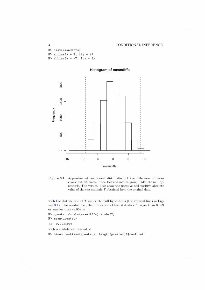
4 CONDITIONAL INFERENCER> hist(meandiffs)R> abline(v = T, lty = 2)R> abline(v = -T, lty = 2)
Histogram of meandiffs
meandiffs
Fre
quen
cy
−15 −10 −5 0 5 10
050
010
0015
0020
00
Figure 3.1 Approximated conditional distribution of the difference of meanroomwidth estimates in the feet and metres group under the null hy-pothesis. The vertical lines show the negative and positive absolutevalue of the test statistic T obtained from the original data.
with the distribution of T under the null hypothesis (the vertical lines in Fig-ure 3.1). The p-value, i.e., the proportion of test statistics T larger than 8.859or smaller than -8.859 isR> greater <- abs(meandiffs) > abs(T)R> mean(greater)
[1] 0.0080008
with a confidence interval ofR> binom.test(sum(greater), length(greater))$conf.int

ANALYSIS USING R 5
[1] 0.006349087 0.009947933attr(,"conf.level")[1] 0.95
Note that the approximated conditional p-value is roughly the same as thep-value reported by the t-test in Chapter 2.
R> library("coin")R> independence_test(y ~ unit, data = roomwidth, distribution = "exact")
Exact General Independence Test
data: y by groups feet, metresZ = -2.5491, p-value = 0.008492alternative hypothesis: two.sided
Figure 3.2 R output of the exact permutation test applied to the roomwidth data.
R> wilcox_test(y ~ unit, data = roomwidth, distribution = "exact")
Exact Wilcoxon Mann-Whitney Rank Sum Test
data: y by groups feet, metresZ = -2.1981, p-value = 0.02763alternative hypothesis: true mu is not equal to 0
Figure 3.3 R output of the exact conditional Wilcoxon rank sum test applied tothe roomwidth data.
3.3.2 Crowds and Threatened Suicide
3.3.3 Gastrointestinal Damages
Here we are interested in the comparison of two groups of patients, where onegroup received a placebo and the other one Misoprostol. In the trials shownhere, the response variable is measured on an ordered scale – see Table ??.Data from four clinical studies are available and thus the observations arenaturally grouped together. From the data.frame Lanza we can construct athree-way table as follows:R> data("Lanza", package = "HSAUR")R> xtabs(~treatment + classification + study, data = Lanza)
, , study = I

6 CONDITIONAL INFERENCE
R> data("suicides", package = "HSAUR")R> fisher.test(suicides)
Fisher's Exact Test for Count Data
data: suicidesp-value = 0.0805alternative hypothesis: true odds ratio is not equal to 195 percent confidence interval:0.7306872 91.0288231
sample estimates:odds ratio6.302622
Figure 3.4 R output of Fisher’s exact test for the suicides data.
classificationtreatment 1 2 3 4 5Misoprostol 21 2 4 2 0Placebo 2 2 4 9 13
, , study = II
classificationtreatment 1 2 3 4 5Misoprostol 20 4 6 0 0Placebo 8 4 9 4 5
, , study = III
classificationtreatment 1 2 3 4 5Misoprostol 20 4 3 1 2Placebo 0 2 5 5 17
, , study = IV
classificationtreatment 1 2 3 4 5Misoprostol 1 4 5 0 0Placebo 0 0 0 4 6
For the first study, the null hypothesis of independence of treatment andgastrointestinal damage, i.e., of no treatment effect of Misoprostol, is testedby
R> library("coin")R> cmh_test(classification ~ treatment, data = Lanza,

ANALYSIS USING R 7
+ scores = list(classification = c(0, 1, 6, 17,+ 30)), subset = Lanza$study == "I")
Asymptotic Linear-by-Linear Association Test
data: classification (ordered) by groups Misoprostol, Placebochi-squared = 28.8478, df = 1, p-value = 7.83e-08
and, by default, the conditional distribution is approximated by the corre-sponding limiting distribution. The p-value indicates a strong treatment effect.For the second study, the asymptotic p-value is a little bit largerR> cmh_test(classification ~ treatment, data = Lanza,+ scores = list(classification = c(0, 1, 6, 17,+ 30)), subset = Lanza$study == "II")
Asymptotic Linear-by-Linear Association Test
data: classification (ordered) by groups Misoprostol, Placebochi-squared = 12.0641, df = 1, p-value = 0.000514
and we make sure that the implied decision is correct by calculating a confi-dence interval for the exact p-valueR> p <- cmh_test(classification ~ treatment, data = Lanza,+ scores = list(classification = c(0, 1, 6, 17,+ 30)), subset = Lanza$study == "II", distribution = approximate(B = 19999))R> pvalue(p)
[1] 5.00025e-0599 percent confidence interval:2.506396e-07 3.714653e-04
The third and fourth study indicate a strong treatment effect as wellR> cmh_test(classification ~ treatment, data = Lanza,+ scores = list(classification = c(0, 1, 6, 17,+ 30)), subset = Lanza$study == "III")
Asymptotic Linear-by-Linear Association Test
data: classification (ordered) by groups Misoprostol, Placebochi-squared = 28.1587, df = 1, p-value = 1.118e-07
R> cmh_test(classification ~ treatment, data = Lanza,+ scores = list(classification = c(0, 1, 6, 17,+ 30)), subset = Lanza$study == "IV")
Asymptotic Linear-by-Linear Association Test
data: classification (ordered) by groups Misoprostol, Placebochi-squared = 15.7414, df = 1, p-value = 7.262e-05
At the end, a separate analysis for each study is unsatisfactory. Because thedesign of the four studies is the same, we can use study as a block variable

8 CONDITIONAL INFERENCE
and perform a global linear-association test investigating the treatment effectof Misoprostol in all four studies. The block variable can be incorporated intothe formula by the | symbol.R> cmh_test(classification ~ treatment | study, data = Lanza,+ scores = list(classification = c(0, 1, 6, 17,+ 30)))
Asymptotic Linear-by-Linear Association Test
data: classification (ordered) bygroups Misoprostol, Placebostratified by study
chi-squared = 83.6188, df = 1, p-value < 2.2e-16
Based on this result, a strong treatment effect can be established.
3.3.4 Teratogenesis
In this example, the medical doctor (MD) and the research assistant (RA)assessed the number of anomalies (0, 1, 2 or 3) for each of 395 babies:R> anomalies <- as.table(matrix(c(235, 23, 3, 0, 41,+ 35, 8, 0, 20, 11, 11, 1, 2, 1, 3, 1), ncol = 4,+ dimnames = list(MD = 0:3, RA = 0:3)))R> anomalies
RAMD 0 1 2 30 235 41 20 21 23 35 11 12 3 8 11 33 0 0 1 1
We are interested in testing whether the number of anomalies assessed by themedical doctor differs structurally from the number reported by the researchassistant. Because we compare paired observations, i.e., one pair of measure-ments for each newborn, a test of marginal homogeneity (a generalisation ofMcNemar’s test, see Chapter 2) needs to be applied:

ANALYSIS USING R 9
R> mh_test(anomalies)
Asymptotic Marginal-Homogeneity Test
data: response bygroups MD, RAstratified by block
chi-squared = 21.2266, df = 3, p-value = 9.446e-05
The p-value indicates a deviation from the null hypothesis. However, the levelsof the response are not treated as ordered. Similar to the analysis of thegastrointestinal damage data above, we can take this information into accountby the definition of an appropriate score. Here, the number of anomalies is anatural choice:R> mh_test(anomalies, scores = list(c(0, 1, 2, 3)))
Asymptotic Marginal-Homogeneity Test for Ordered Data
data: response (ordered) bygroups MD, RAstratified by block
chi-squared = 21.0199, df = 1, p-value = 4.545e-06
In our case, both versions coincide and one can conclude that the assessment ofthe number of anomalies differs between the medical doctor and the researchassistant.

CHAPTER 4
Analysis of Variance: Weight Gain,Foster Feeding in Rats, Water
Hardness and Male Egyptian Skulls
4.1 Introduction
4.2 Analysis of Variance
4.3 Analysis Using R
4.3.1 Weight Gain in Rats
Before applying analysis of variance to the data in Table ?? we should try tosummarise the main features of the data by calculating means and standarddeviations and by producing some hopefully informative graphs. The data isavailable in the data.frame weightgain. The following R code produces therequired summary statisticsR> data("weightgain", package = "HSAUR")R> tapply(weightgain$weightgain, list(weightgain$source,+ weightgain$type), mean)
High LowBeef 100.0 79.2Cereal 85.9 83.9
R> tapply(weightgain$weightgain, list(weightgain$source,+ weightgain$type), sd)
High LowBeef 15.13642 13.88684Cereal 15.02184 15.70881
To apply analysis of variance to the data we can use the aov function in Rand then the summary method to give us the usual analysis of variance table.The model formula specifies a two-way layout with interaction terms, wherethe first factor is source, and the second factor is type.R> wg_aov <- aov(weightgain ~ source * type, data = weightgain)
The estimates of the intercept and the main and interaction effects can beextracted from the model fit byR> coef(wg_aov)
(Intercept) sourceCereal typeLow100.0 -14.1 -20.8
3
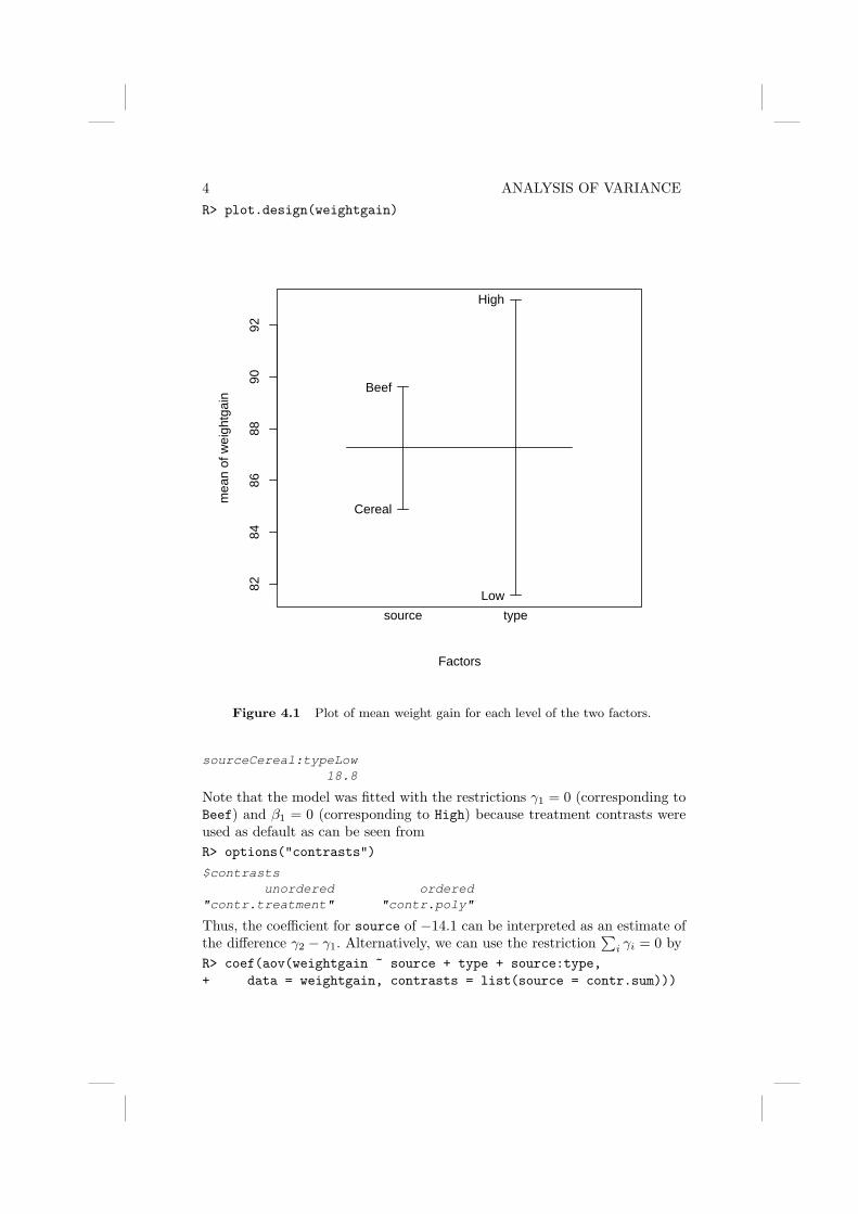
4 ANALYSIS OF VARIANCER> plot.design(weightgain)
8284
8688
9092
Factors
mea
n of
wei
ghtg
ain
Beef
Cereal
High
Low
source type
Figure 4.1 Plot of mean weight gain for each level of the two factors.
sourceCereal:typeLow18.8
Note that the model was fitted with the restrictions γ1 = 0 (corresponding toBeef) and β1 = 0 (corresponding to High) because treatment contrasts wereused as default as can be seen fromR> options("contrasts")
$contrastsunordered ordered
"contr.treatment" "contr.poly"
Thus, the coefficient for source of −14.1 can be interpreted as an estimate ofthe difference γ2 − γ1. Alternatively, we can use the restriction
∑i γi = 0 by
R> coef(aov(weightgain ~ source + type + source:type,+ data = weightgain, contrasts = list(source = contr.sum)))

ANALYSIS USING R 5
R> summary(wg_aov)
Df Sum Sq Mean Sq F value Pr(>F)source 1 220.9 220.9 0.9879 0.32688type 1 1299.6 1299.6 5.8123 0.02114 *source:type 1 883.6 883.6 3.9518 0.05447 .Residuals 36 8049.4 223.6---Signif. codes: 0 '***' 0.001 '**' 0.01 '*' 0.05 '.' 0.1 ' ' 1
Figure 4.2 R output of the ANOVA fit for the weightgain data.
(Intercept) source1 typeLow92.95 7.05 -11.40
source1:typeLow-9.40
4.3.2 Foster Feeding of Rats of Different Genotype
As in the previous subsection we will begin the analysis of the foster feedingdata in Table ?? with a plot of the mean litter weight for the different geno-types of mother and litter (see Figure 4.4). The data are in the data.framefoster
R> data("foster", package = "HSAUR")
We can derive the two analyses of variance tables for the foster feeding exampleby applying the R codeR> summary(aov(weight ~ litgen * motgen, data = foster))
to giveDf Sum Sq Mean Sq F value Pr(>F)
litgen 3 60.16 20.05 0.3697 0.775221motgen 3 775.08 258.36 4.7632 0.005736 **litgen:motgen 9 824.07 91.56 1.6881 0.120053Residuals 45 2440.82 54.24---Signif. codes: 0 '***' 0.001 '**' 0.01 '*' 0.05 '.' 0.1 ' ' 1
and then the codeR> summary(aov(weight ~ motgen * litgen, data = foster))
to giveDf Sum Sq Mean Sq F value Pr(>F)
motgen 3 771.61 257.20 4.7419 0.005869 **litgen 3 63.63 21.21 0.3911 0.760004motgen:litgen 9 824.07 91.56 1.6881 0.120053Residuals 45 2440.82 54.24---Signif. codes: 0 '***' 0.001 '**' 0.01 '*' 0.05 '.' 0.1 ' ' 1

6 ANALYSIS OF VARIANCER> interaction.plot(weightgain$type, weightgain$source,+ weightgain$weightgain)
8085
9095
100
weightgain$type
mea
n of
wei
ghtg
ain$
wei
ghtg
ain
High Low
weightgain$source
BeefCereal
Figure 4.3 Interaction plot of type × source.
There are (small) differences in the sum of squares for the two main effectsand, consequently, in the associated F -tests and p-values. This would not betrue if in the previous example in Subsection 4.3.1 we had used the code
R> summary(aov(weightgain ~ type * source, data = weightgain))
instead of the code which produced Figure 4.2 (readers should confirm thatthis is the case). We can investigate the effect of genotype B on litter weight inmore detail by the use of multiple comparison procedures (see Everitt, 1996).Such procedures allow a comparison of all pairs of levels of a factor whilstmaintaining the nominal significance level at its selected value and producingadjusted confidence intervals for mean differences. One such procedure is calledTukey honest significant differences suggested by Tukey (1953), see Hochbergand Tamhane (1987) also. Here, we are interested in simultaneous confidence

ANALYSIS USING R 7R> plot.design(foster)
5052
5456
58
Factors
mea
n of
wei
ght A
B
IJ
A
B
I
J
litgen motgen
Figure 4.4 Plot of mean litter weight for each level of the two factors for thefoster data.
intervals for the weight differences between all four genotypes of the mother.First, an ANOVA model is fitted
R> foster_aov <- aov(weight ~ litgen * motgen, data = foster)
which serves as the basis of the multiple comparisons, here with allpair differ-ences by
R> foster_hsd <- TukeyHSD(foster_aov, "motgen")R> foster_hsd
Tukey multiple comparisons of means95% family-wise confidence level
Fit: aov(formula = weight ~ litgen * motgen, data = foster)

8 ANALYSIS OF VARIANCER> plot(foster_hsd)
−15 −10 −5 0 5 10
J−I
J−B
I−B
J−A
I−A
B−
A95% family−wise confidence level
Differences in mean levels of motgen
Figure 4.5 Graphical presentation of multiple comparison results for the foster
feeding data.
$motgendiff lwr upr p adj
B-A 3.330369 -3.859729 10.5204672 0.6078581I-A -1.895574 -8.841869 5.0507207 0.8853702J-A -6.566168 -13.627285 0.4949498 0.0767540I-B -5.225943 -12.416041 1.9641552 0.2266493J-B -9.896537 -17.197624 -2.5954489 0.0040509J-I -4.670593 -11.731711 2.3905240 0.3035490
A convenient plot method exists for this object and we can get a graphicalrepresentation of the multiple confidence intervals as shown in Figure 4.5. Itappears that there is only evidence for a difference in the B and J genotypes.

ANALYSIS USING R 9
4.3.3 Water Hardness and Mortality
The water hardness and mortality data for 61 large towns in England andWales (see Table 2.3) was analysed in Chapter 2 and here we will extend theanalysis by an assessment of the differences of both hardness and mortalityin the North or South. The hypothesis that the two-dimensional mean-vectorof water hardness and mortality is the same for cities in the North and theSouth can be tested by Hotelling-Lawley test in a multivariate analysis ofvariance framework. The R function manova can be used to fit such a modeland the corresponding summary method performs the test specified by thetest argumentR> data("water", package = "HSAUR")R> summary(manova(cbind(hardness, mortality) ~ location,+ data = water), test = "Hotelling-Lawley")
Df Hotelling-Lawley approx F num Df den Df Pr(>F)location 1 0.9002 26.1062 2 58 8.217e-09Residuals 59
location ***Residuals---Signif. codes: 0 '***' 0.001 '**' 0.01 '*' 0.05 '.' 0.1 ' ' 1
The cbind statement in the left hand side of the formula indicates that amultivariate response variable is to be modelled. The p-value associated withthe Hotelling-Lawley statistic is very small and there is strong evidence thatthe mean vectors of the two variables are not the same in the two regions.Looking at the sample meansR> tapply(water$hardness, water$location, mean)
North South30.40000 69.76923
R> tapply(water$mortality, water$location, mean)
North South1633.600 1376.808
we see large differences in the two regions both in water hardness and mortal-ity, where low mortality is associated with hard water in the South and highmortality with soft water in the North (see Figure ?? also).
4.3.4 Male Egyptian Skulls
We can begin by looking at a table of mean values for the four measure-ments within each of the five epochs. The measurements are available in thedata.frame skulls and we can compute the means over all epochs byR> data("skulls", package = "HSAUR")R> means <- aggregate(skulls[, c("mb", "bh", "bl",

10 ANALYSIS OF VARIANCER> pairs(means[, -1], panel = function(x, y) {+ text(x, y, abbreviate(levels(skulls$epoch)))+ })
mb
130.5 132.0 133.5
c400
c330
c185
c200cAD1
c400
c330
c185
c200cAD1
50.5 51.5
132
134
136
c400
c330
c185
c200cAD1
130.
513
2.0
133.
5
c400
c330
c185
c200
cAD1
bh
c400
c330
c185
c200
cAD1
c400
c330
c185
c200
cAD1
c400c330
c185
c200
cAD1
c400c330
c185
c200
cAD1
bl
9496
98
c400c330
c185
c200
cAD1
132 134 136
50.5
51.5
c400
c330
c185
c200
cAD1
c400
c330
c185
c200
cAD1
94 96 98
c400
c330
c185
c200
cAD1
nh
Figure 4.6 Scatterplot matrix of epoch means for Egyptian skulls data.
+ "nh")], list(epoch = skulls$epoch), mean)R> means
epoch mb bh bl nh1 c4000BC 131.3667 133.6000 99.16667 50.533332 c3300BC 132.3667 132.7000 99.06667 50.233333 c1850BC 134.4667 133.8000 96.03333 50.566674 c200BC 135.5000 132.3000 94.53333 51.966675 cAD150 136.1667 130.3333 93.50000 51.36667
It may also be useful to look at these means graphically and this could be donein a variety of ways. Here we construct a scatterplot matrix of the means usingthe code attached to Figure 4.6. There appear to be quite large differences

ANALYSIS USING R 11
between the epoch means, at least on some of the four measurements. We cannow test for a difference more formally by using MANOVA with the followingR code to apply each of the four possible test criteria mentioned earlier;R> skulls_manova <- manova(cbind(mb, bh, bl, nh) ~+ epoch, data = skulls)R> summary(skulls_manova, test = "Pillai")
Df Pillai approx F num Df den Df Pr(>F)epoch 4 0.3533 3.5120 16 580 4.675e-06 ***Residuals 145---Signif. codes: 0 '***' 0.001 '**' 0.01 '*' 0.05 '.' 0.1 ' ' 1
R> summary(skulls_manova, test = "Wilks")
Df Wilks approx F num Df den Df Pr(>F)epoch 4.00 0.6636 3.9009 16.00 434.45 7.01e-07 ***Residuals 145.00---Signif. codes: 0 '***' 0.001 '**' 0.01 '*' 0.05 '.' 0.1 ' ' 1
R> summary(skulls_manova, test = "Hotelling-Lawley")
Df Hotelling-Lawley approx F num Df den Dfepoch 4 0.4818 4.2310 16 562Residuals 145
Pr(>F)epoch 8.278e-08 ***Residuals---Signif. codes: 0 '***' 0.001 '**' 0.01 '*' 0.05 '.' 0.1 ' ' 1
R> summary(skulls_manova, test = "Roy")
Df Roy approx F num Df den Df Pr(>F)epoch 4 0.4251 15.4097 4 145 1.588e-10 ***Residuals 145---Signif. codes: 0 '***' 0.001 '**' 0.01 '*' 0.05 '.' 0.1 ' ' 1
The p-value associated with each four test criteria is very small and there isstrong evidence that the skull measurements differ between the five epochs. Wemight now move on to investigate which epochs differ and on which variables.We can look at the univariate F -tests for each of the four variables by usingthe codeR> summary.aov(manova(cbind(mb, bh, bl, nh) ~ epoch,+ data = skulls))
Response mb :Df Sum Sq Mean Sq F value Pr(>F)
epoch 4 502.83 125.71 5.9546 0.0001826 ***Residuals 145 3061.07 21.11---

12 ANALYSIS OF VARIANCE
Signif. codes: 0 '***' 0.001 '**' 0.01 '*' 0.05 '.' 0.1 ' ' 1
Response bh :Df Sum Sq Mean Sq F value Pr(>F)
epoch 4 229.9 57.5 2.4474 0.04897 *Residuals 145 3405.3 23.5---Signif. codes: 0 '***' 0.001 '**' 0.01 '*' 0.05 '.' 0.1 ' ' 1
Response bl :Df Sum Sq Mean Sq F value Pr(>F)
epoch 4 803.3 200.8 8.3057 4.636e-06 ***Residuals 145 3506.0 24.2---Signif. codes: 0 '***' 0.001 '**' 0.01 '*' 0.05 '.' 0.1 ' ' 1
Response nh :Df Sum Sq Mean Sq F value Pr(>F)
epoch 4 61.20 15.30 1.507 0.2032Residuals 145 1472.13 10.15
We see that the results for the maximum breadths (mb) and basialiveolar length(bl) are highly significant, with those for the other two variables, in particularfor nasal heights (nh), suggesting little evidence of a difference. To look at thepairwise multivariate tests (any of the four test criteria are equivalent in thecase of a one-way layout with two levels only) we can use the summary methodand manova function as follows:R> summary(manova(cbind(mb, bh, bl, nh) ~ epoch, data = skulls,+ subset = epoch %in% c("c4000BC", "c3300BC")))
Df Pillai approx F num Df den Df Pr(>F)epoch 1 0.02767 0.39135 4 55 0.814Residuals 58
R> summary(manova(cbind(mb, bh, bl, nh) ~ epoch, data = skulls,+ subset = epoch %in% c("c4000BC", "c1850BC")))
Df Pillai approx F num Df den Df Pr(>F)epoch 1 0.1876 3.1744 4 55 0.02035 *Residuals 58---Signif. codes: 0 '***' 0.001 '**' 0.01 '*' 0.05 '.' 0.1 ' ' 1
R> summary(manova(cbind(mb, bh, bl, nh) ~ epoch, data = skulls,+ subset = epoch %in% c("c4000BC", "c200BC")))
Df Pillai approx F num Df den Df Pr(>F)epoch 1 0.3030 5.9766 4 55 0.0004564 ***Residuals 58---Signif. codes: 0 '***' 0.001 '**' 0.01 '*' 0.05 '.' 0.1 ' ' 1

ANALYSIS USING R 13
R> summary(manova(cbind(mb, bh, bl, nh) ~ epoch, data = skulls,+ subset = epoch %in% c("c4000BC", "cAD150")))
Df Pillai approx F num Df den Df Pr(>F)epoch 1 0.3618 7.7956 4 55 4.736e-05 ***Residuals 58---Signif. codes: 0 '***' 0.001 '**' 0.01 '*' 0.05 '.' 0.1 ' ' 1
To keep the overall significance level for the set of all pairwise multivariatetests under some control (and still maintain a reasonable power), Stevens(2001) recommends setting the nominal level α = 0.15 and carrying out eachtest at the α/m level where m s the number of tests performed. The resultsof the four pairwise tests suggest that as the epochs become further separatedin time the four skull measurements become increasingly distinct.


Bibliography
Everitt, B. S. (1996), Making Sense of Statistics in Psychology: A Second-LevelCourse, Oxford, UK: Oxford University Press.
Hochberg, Y. and Tamhane, A. C. (1987), Multiple Comparison Procedures,New York, USA: John Wiley & Sons.
Stevens, J. (2001), Applied Multivariate Statistics for the Social Sciences,Mahwah, New Jersey, USA: Lawrence Erlbaum, 4th edition.
Tukey, J. W. (1953), “The problem of multiple comparisons (unpublishedmanuscript),” in The Collected Works of John W. Tukey VIII. MultipleComparisons: 1948-1983 , New York, USA: Chapman & Hall.

CHAPTER 5
Multiple Linear Regression: CloudSeeding
5.1 Introduction
5.2 Multiple Linear Regression
5.3 Analysis Using R
Both the boxplots (Figure 5.1) and the scatterplots (Figure 5.2) show someevidence of outliers. The row names of the extreme observations in the cloudsdata.frame can be identified viaR> rownames(clouds)[clouds$rainfall %in% c(bxpseeding$out,+ bxpecho$out)]
[1] "1" "15"
where bxpseeding and bxpecho are variables created by boxplot in Fig-ure 5.1. For the time being we shall not remove these observations but bearin mind during the modelling process that they may cause problems.
5.3.1 Fitting a Linear Model
In this example it is sensible to assume that the effect that some of the otherexplanatory variables is modified by seeding and therefore consider a modelthat allows interaction terms for seeding with each of the covariates excepttime. This model can be described by the formulaR> clouds_formula <- rainfall ~ seeding * (sne + cloudcover ++ prewetness + echomotion) + time
and the design matrix X? can be computed viaR> Xstar <- model.matrix(clouds_formula, data = clouds)
By default, treatment contrasts have been applied to the dummy codings ofthe factors seeding and echomotion as can be seen from the inspection ofthe contrasts attribute of the model matrixR> attr(Xstar, "contrasts")
$seeding[1] "contr.treatment"
$echomotion[1] "contr.treatment"
3
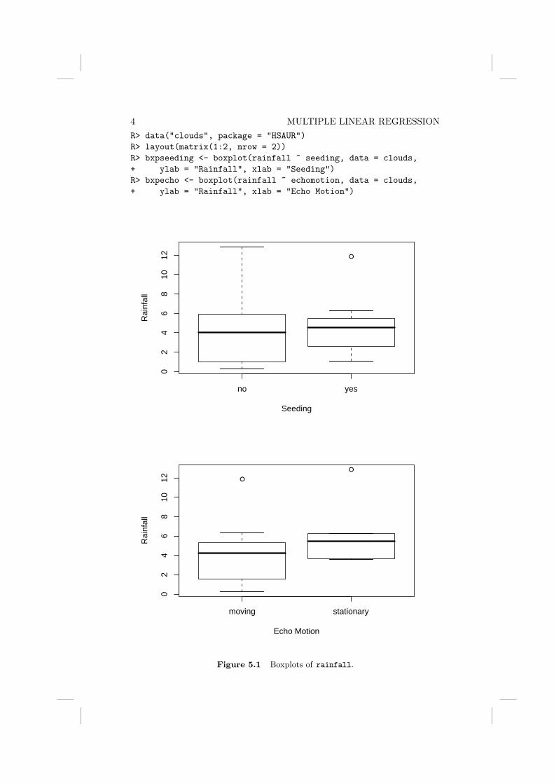
4 MULTIPLE LINEAR REGRESSIONR> data("clouds", package = "HSAUR")R> layout(matrix(1:2, nrow = 2))R> bxpseeding <- boxplot(rainfall ~ seeding, data = clouds,+ ylab = "Rainfall", xlab = "Seeding")R> bxpecho <- boxplot(rainfall ~ echomotion, data = clouds,+ ylab = "Rainfall", xlab = "Echo Motion")
●
no yes
02
46
810
12
Seeding
Rai
nfal
l
●
●
moving stationary
02
46
810
12
Echo Motion
Rai
nfal
l
Figure 5.1 Boxplots of rainfall.

ANALYSIS USING R 5R> layout(matrix(1:4, nrow = 2))R> plot(rainfall ~ time, data = clouds)R> plot(rainfall ~ sne, data = clouds, xlab = "S-NE criterion")R> plot(rainfall ~ cloudcover, data = clouds)R> plot(rainfall ~ prewetness, data = clouds)
●
●
●●
●
●
●
●
●
●
●
●
●
●
●
●
●●
●
●
●
● ●
●
0 20 40 60 80
02
46
810
12
time
rain
fall
●
●
● ●
●
●
●
●
●
●
●
●
●
●
●
●
●●
●
●
●
● ●
●
5 10 15 20 25 30 35
02
46
810
12
S−NE criterion
rain
fall
●
●
●●
●
●
●
●
●
●
●
●
●
●
●
●
●●
●
●
●
● ●
●
1.5 2.0 2.5 3.0 3.5 4.0 4.50
24
68
1012
cloudcover
rain
fall
●
●
● ●
●
●
●
●
●
●
●
●
●
●
●
●
●●
●
●
●
●●
●
0.0 0.2 0.4 0.6 0.8 1.0 1.2
02
46
810
12
prewetness
rain
fall
Figure 5.2 Scatterplots of rainfall against the continuous covariables.
The default contrasts can be changed via the contrasts.arg argument tomodel.matrix or the contrasts argument to the fitting function, for examplelm or aov as shown in Chapter 4. However, such internals are hidden andperformed by high-level model fitting functions such as lm which will be usedto fit the linear model defined by the formula clouds_formula:
R> clouds_lm <- lm(clouds_formula, data = clouds)R> class(clouds_lm)
[1] "lm"

6 MULTIPLE LINEAR REGRESSION
The results of the model fitting is an object of class lm for which a summarymethod showing the conventional regression analysis output is available. Theoutput in Figure 5.3 shows the estimates β? with corresponding standarderrors and t-statistics as well as the F -statistic with associated p-value.
R> summary(clouds_lm)
Call:lm(formula = clouds_formula, data = clouds)
Residuals:Min 1Q Median 3Q Max
-2.5259 -1.1486 -0.2704 1.0401 4.3913
Coefficients:Estimate Std. Error t value
(Intercept) -0.34624 2.78773 -0.124seedingyes 15.68293 4.44627 3.527sne 0.38786 0.21786 1.780cloudcover 0.41981 0.84453 0.497prewetness 4.10834 3.60101 1.141echomotionstationary 3.15281 1.93253 1.631time -0.04497 0.02505 -1.795seedingyes:sne -0.48625 0.24106 -2.017seedingyes:cloudcover -3.19719 1.26707 -2.523seedingyes:prewetness -2.55707 4.48090 -0.571seedingyes:echomotionstationary -0.56222 2.64430 -0.213
Pr(>|t|)(Intercept) 0.90306seedingyes 0.00372 **sne 0.09839 .cloudcover 0.62742prewetness 0.27450echomotionstationary 0.12677time 0.09590 .seedingyes:sne 0.06482 .seedingyes:cloudcover 0.02545 *seedingyes:prewetness 0.57796seedingyes:echomotionstationary 0.83492---Signif. codes: 0 '***' 0.001 '**' 0.01 '*' 0.05 '.' 0.1 ' ' 1
Residual standard error: 2.205 on 13 degrees of freedomMultiple R-Squared: 0.7158, Adjusted R-squared: 0.4972F-statistic: 3.274 on 10 and 13 DF, p-value: 0.02431
Figure 5.3 R output of the linear model fit for the clouds data.

ANALYSIS USING R 7
Many methods are available for extracting components of the fitted model.The estimates β? can be assessed viaR> betastar <- coef(clouds_lm)R> betastar
(Intercept)-0.34624093seedingyes15.68293481
sne0.38786207cloudcover0.41981393prewetness4.10834188
echomotionstationary3.15281358
time-0.04497427
seedingyes:sne-0.48625492
seedingyes:cloudcover-3.19719006
seedingyes:prewetness-2.55706696
seedingyes:echomotionstationary-0.56221845
and the corresponding covariance matrix Cov(β?) is available from the vcovmethodR> Vbetastar <- vcov(clouds_lm)
where the square roots of the diagonal elements are the standard errors asshown in Figure 5.3R> sqrt(diag(Vbetastar))
(Intercept)2.78773403seedingyes4.44626606
sne0.21785501cloudcover0.84452994prewetness3.60100694
echomotionstationary1.93252592
time0.02505286

8 MULTIPLE LINEAR REGRESSION
seedingyes:sne0.24106012
seedingyes:cloudcover1.26707204
seedingyes:prewetness4.48089584
seedingyes:echomotionstationary2.64429975
5.3.2 Regression Diagnostics
In order to investigate the quality of the model fit, we need access to theresiduals and the fitted values. The residuals can be found by the residualsmethod and the fitted values of the response from the fitted (or predict)methodR> clouds_resid <- residuals(clouds_lm)R> clouds_fitted <- fitted(clouds_lm)
Now the residuals and the fitted values can be used to construct diagnosticplots; for example the residual plot in Figure 5.5 where each observation islabelled by its number. Observations 1 and 15 give rather large residual valuesand the data should perhaps be reanalysed after these two observations areremoved. The normal probability plot of the residuals shown in Figure 5.6shows a reasonable agreement between theoretical and sample quantiles, how-ever, observations 1 and 15 are extreme again. An index plot of the Cook’sdistances for each observation (and many other plots including those con-structed above from using the basic functions) can be found from applyingthe plot method to the object that results from the application of the lmfunction. Figure 5.7 suggests that observations 2 and 18 have undue influenceon the estimated regression coefficients, but the two outliers identified previ-ously do not. Again it may be useful to look at the results after these twoobservations have been removed (see Exercise 5.2).
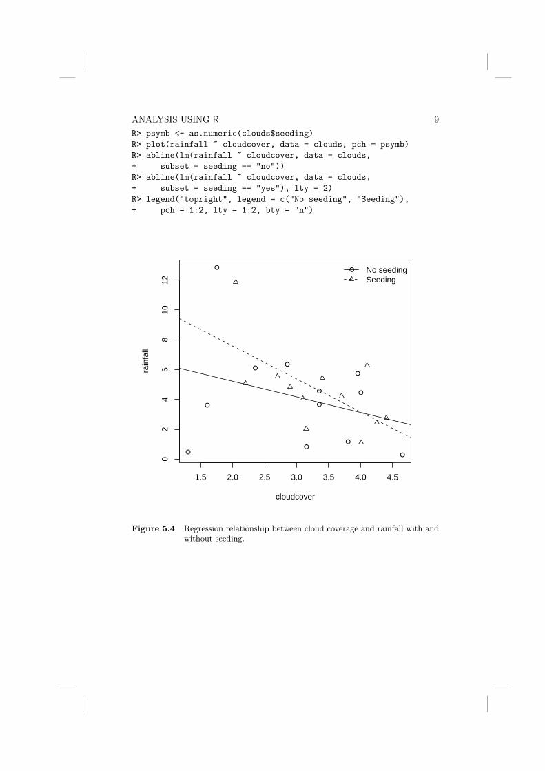
ANALYSIS USING R 9R> psymb <- as.numeric(clouds$seeding)R> plot(rainfall ~ cloudcover, data = clouds, pch = psymb)R> abline(lm(rainfall ~ cloudcover, data = clouds,+ subset = seeding == "no"))R> abline(lm(rainfall ~ cloudcover, data = clouds,+ subset = seeding == "yes"), lty = 2)R> legend("topright", legend = c("No seeding", "Seeding"),+ pch = 1:2, lty = 1:2, bty = "n")
●
●
●
●
●
●
●
●
●
●●
●
1.5 2.0 2.5 3.0 3.5 4.0 4.5
02
46
810
12
cloudcover
rain
fall
● No seedingSeeding
Figure 5.4 Regression relationship between cloud coverage and rainfall with andwithout seeding.

10 MULTIPLE LINEAR REGRESSIONR> plot(clouds_fitted, clouds_resid, xlab = "Fitted values",+ ylab = "Residuals", ylim = max(abs(clouds_resid)) *+ c(-1, 1), type = "n")R> abline(h = 0, lty = 2)R> text(clouds_fitted, clouds_resid, labels = rownames(clouds))
0 2 4 6 8 10
−4
−2
02
4
Fitted values
Res
idua
ls
1
23
4
5
67
8
9
10
11
12
13
14
15
1617
1819
20
21
2223
24
Figure 5.5 Plot of residuals against fitted values for clouds seeding data.

ANALYSIS USING R 11R> qqnorm(clouds_resid, ylab = "Residuals")R> qqline(clouds_resid)
●
●
●
●
●
●
●
●
●
●
●
●
●
●
●
●
●
●●
●
●
●●
●
−2 −1 0 1 2
−2
−1
01
23
4Normal Q−Q Plot
Theoretical Quantiles
Res
idua
ls
Figure 5.6 Normal probability plot of residuals from cloud seeding modelclouds_lm.

12 MULTIPLE LINEAR REGRESSIONR> plot(clouds_lm)
5 10 15 20
02
46
8
Obs. number
Coo
k's
dist
ance
lm(clouds_formula)
Cook's distance
2
18
1
Figure 5.7 Index plot of Cook’s distances for cloud seeding data.
CHAPTER 6
Logistic Regression and GeneralisedLinear Models: Blood Screening,
Women’s Role in Society,and Colonic Polyps
6.1 Introduction
6.2 Logistic Regression and Generalised Linear Models
6.3 Analysis Using R
6.3.1 ESR and Plasma Proteins
We can now fit a logistic regression model to the data using the glm func-tion. We start with a model that includes only a single explanatory variable,fibrinogen. The code to fit the model is
R> plasma_glm_1 <- glm(ESR ~ fibrinogen, data = plasma,+ family = binomial())
The formula implicitly defines a parameter for the global mean (the interceptterm) as discussed in Chapters ?? and ??. The distribution of the responseis defined by the family argument, a binomial distribution in our case. (Thedefault link function when the binomial family is requested is the logisticfunction.) From the results in Figure 6.2 we see that the regressioncoefficient for fibrinogen is significant at the 5% level. An increase of one unitin this variable increases the log-odds in favour of an ESR value greater than20 by an estimated 1.83 with 95% confidence interval
R> confint(plasma_glm_1, parm = "fibrinogen")
2.5 % 97.5 %0.3389465 3.9988602
These values are more helpful if converted to the corresponding values for theodds themselves by exponentiating the estimate
R> exp(coef(plasma_glm_1)["fibrinogen"])
fibrinogen6.215715
and the confidence interval
R> exp(confint(plasma_glm_1, parm = "fibrinogen"))
3

4 LOGISTIC REGRESSION AND GENERALISED LINEAR MODELSR> data("plasma", package = "HSAUR")R> layout(matrix(1:2, ncol = 2))R> cdplot(ESR ~ fibrinogen, data = plasma)R> cdplot(ESR ~ globulin, data = plasma)
fibrinogen
ES
R
2.5 3.5 4.5
ES
R <
20
ES
R >
20
0.0
0.2
0.4
0.6
0.8
1.0
globulin
ES
R
30 35 40 45
ES
R <
20
ES
R >
20
0.0
0.2
0.4
0.6
0.8
1.0
Figure 6.1 Conditional density plots of the erythrocyte sedimentation rate (ESR)given fibrinogen and globulin.
2.5 % 97.5 %1.403468 54.535954
The confidence interval is very wide because there are few observations overalland very few where the ESR value is greater than 20. Nevertheless it seemslikely that increased values of fibrinogen lead to a greater probability of anESR value greater than 20. We can now fit a logistic regression model thatincludes both explanatory variables using the codeR> plasma_glm_2 <- glm(ESR ~ fibrinogen + globulin,+ data = plasma, family = binomial())
and the output of the summary method is shown in Figure 6.3. Thecoefficient for gamma globulin is not significantly different from zero. Sub-tracting the residual deviance of the second model from the correspondingvalue for the first model we get a value of 1.87. Tested using a χ2-distributionwith a single degree of freedom this is not significant at the 5% level and sowe conclude that gamma globulin is not associated with ESR level. In R, thetask of comparing the two nested models can be performed using the anovafunctionR> anova(plasma_glm_1, plasma_glm_2, test = "Chisq")

ANALYSIS USING R 5
R> summary(plasma_glm_1)
Call:glm(formula = ESR ~ fibrinogen, family = binomial(), data = plasma)
Deviance Residuals:Min 1Q Median 3Q Max
-0.9298 -0.5399 -0.4382 -0.3356 2.4794
Coefficients:Estimate Std. Error z value Pr(>|z|)
(Intercept) -6.8451 2.7703 -2.471 0.0135 *fibrinogen 1.8271 0.9009 2.028 0.0425 *---Signif. codes: 0 '***' 0.001 '**' 0.01 '*' 0.05 '.' 0.1 ' ' 1
(Dispersion parameter for binomial family taken to be 1)
Null deviance: 30.885 on 31 degrees of freedomResidual deviance: 24.840 on 30 degrees of freedomAIC: 28.840
Number of Fisher Scoring iterations: 5
Figure 6.2 R output of the summary method for the logistic regression model fittedto the plasma data.
Analysis of Deviance Table
Model 1: ESR ~ fibrinogenModel 2: ESR ~ fibrinogen + globulinResid. Df Resid. Dev Df Deviance P(>|Chi|)
1 30 24.84042 29 22.9711 1 1.8692 0.1716
Nevertheless we shall use the predicted values from the second model and plotthem against the values of both explanatory variables using a bubble plot toillustrate the use of the symbols function. The estimated conditional proba-bility of a ESR value larger 20 for all observations can be computed, followingformula (??), by
R> prob <- predict(plasma_glm_1, type = "response")
and now we can assign a larger circle to observations with larger probabilityas shown in Figure 6.4. The plot clearly shows the increasing probability ofan ESR value above 20 (larger circles) as the values of fibrinogen, and to alesser extent, gamma globulin, increase.
6 LOGISTIC REGRESSION AND GENERALISED LINEAR MODELS
R> summary(plasma_glm_2)
Call:glm(formula = ESR ~ fibrinogen + globulin, family = binomial(),
data = plasma)
Deviance Residuals:Min 1Q Median 3Q Max
-0.9683 -0.6122 -0.3458 -0.2116 2.2636
Coefficients:Estimate Std. Error z value Pr(>|z|)
(Intercept) -12.7921 5.7963 -2.207 0.0273 *fibrinogen 1.9104 0.9710 1.967 0.0491 *globulin 0.1558 0.1195 1.303 0.1925---Signif. codes: 0 '***' 0.001 '**' 0.01 '*' 0.05 '.' 0.1 ' ' 1
(Dispersion parameter for binomial family taken to be 1)
Null deviance: 30.885 on 31 degrees of freedomResidual deviance: 22.971 on 29 degrees of freedomAIC: 28.971
Number of Fisher Scoring iterations: 5
Figure 6.3 R output of the summary method for the logistic regression model fittedto the plasma data.
6.3.2 Women’s Role in Society
Originally the data in Table ?? would have been in a completely equivalentform to the data in Table ?? data, but here the individual observations havebeen grouped into counts of numbers of agreements and disagreements forthe two explanatory variables, sex and education. To fit a logistic regressionmodel to such grouped data using the glm function we need to specify thenumber of agreements and disagreements as a two-column matrix on the lefthand side of the model formula. We first fit a model that includes the twoexplanatory variables using the codeR> data("womensrole", package = "HSAUR")R> womensrole_glm_1 <- glm(cbind(agree, disagree) ~+ sex + education, data = womensrole, family = binomial())
From the summary output in Figure 6.5 it appears that education has a highlysignificant part to play in predicting whether a respondent will agree with thestatement read to them, but the respondent’s sex is apparently unimportant.As years of education increase the probability of agreeing with the statementdeclines. We now are going to construct a plot comparing the observed pro-

ANALYSIS USING R 7R> plot(globulin ~ fibrinogen, data = plasma, xlim = c(2,+ 6), ylim = c(25, 50), pch = ".")R> symbols(plasma$fibrinogen, plasma$globulin, circles = prob,+ add = TRUE)
2 3 4 5 6
2530
3540
4550
fibrinogen
glob
ulin
●
●●
●
●●
●
●
●
●
●●
●
●
●
●●
●
●
●
Figure 6.4 Bubble plot of fitted values for a logistic regression model fitted to theESR data.
portions of agreeing with those fitted by our fitted model. Because we willreuse this plot for another fitted object later on, we define a function whichplots years of education against some fitted probabilities, e.g.,
R> role.fitted1 <- predict(womensrole_glm_1, type = "response")
and labels each observation with the person’s sex:
R> myplot <- function(role.fitted) {+ f <- womensrole$sex == "Female"+ plot(womensrole$education, role.fitted, type = "n",+ ylab = "Probability of agreeing", xlab = "Education",

8 LOGISTIC REGRESSION AND GENERALISED LINEAR MODELS
R> summary(womensrole_glm_1)
Call:glm(formula = cbind(agree, disagree) ~ sex + education, family = binomial(),
data = womensrole)
Deviance Residuals:Min 1Q Median 3Q Max
-2.72544 -0.86302 -0.06525 0.84340 3.13315
Coefficients:Estimate Std. Error z value Pr(>|z|)
(Intercept) 2.50937 0.18389 13.646 <2e-16 ***sexFemale -0.01145 0.08415 -0.136 0.892education -0.27062 0.01541 -17.560 <2e-16 ***---Signif. codes: 0 '***' 0.001 '**' 0.01 '*' 0.05 '.' 0.1 ' ' 1
(Dispersion parameter for binomial family taken to be 1)
Null deviance: 451.722 on 40 degrees of freedomResidual deviance: 64.007 on 38 degrees of freedomAIC: 208.07
Number of Fisher Scoring iterations: 4
Figure 6.5 R output of the summary method for the logistic regression model fittedto the womensrole data.
+ ylim = c(0, 1))+ lines(womensrole$education[!f], role.fitted[!f],+ lty = 1)+ lines(womensrole$education[f], role.fitted[f],+ lty = 2)+ lgtxt <- c("Fitted (Males)", "Fitted (Females)")+ legend("topright", lgtxt, lty = 1:2, bty = "n")+ y <- womensrole$agree/(womensrole$agree + womensrole$disagree)+ text(womensrole$education, y, ifelse(f, "\\VE",+ "\\MA"), family = "HersheySerif", cex = 1.25)+ }
The two curves for males and females in Figure 6.6 are almost the samereflecting the non-significant value of the regression coefficient for sex in wom-ensrole_glm_1. But the observed values plotted on Figure 6.6 suggest thatthere might be an interaction of education and sex, a possibility that can beinvestigated by applying a further logistic regression model using

ANALYSIS USING R 9R> myplot(role.fitted1)
0 5 10 15 20
0.0
0.2
0.4
0.6
0.8
1.0
Education
Pro
babi
lity
of a
gree
ing
Fitted (Males)Fitted (Females)
Figure 6.6 Fitted (from womensrole_glm_1) and observed probabilities of agree-ing for the womensrole data.
R> womensrole_glm_2 <- glm(cbind(agree, disagree) ~+ sex * education, data = womensrole, family = binomial())
The sex and education interaction term is seen to be highly significant, ascan be seen from the summary output in Figure 6.7. We can obtaina plot of deviance residuals plotted against fitted values using the followingcode above Figure 6.9. The residuals fall into a horizontal band between −2and 2. This pattern does not suggest a poor fit for any particular observationor subset of observations.

10 LOGISTIC REGRESSION AND GENERALISED LINEAR MODELS
R> summary(womensrole_glm_2)
Call:glm(formula = cbind(agree, disagree) ~ sex * education, family = binomial(),
data = womensrole)
Deviance Residuals:Min 1Q Median 3Q Max
-2.39097 -0.88062 0.01532 0.72783 2.45262
Coefficients:Estimate Std. Error z value Pr(>|z|)
(Intercept) 2.09820 0.23550 8.910 < 2e-16 ***sexFemale 0.90474 0.36007 2.513 0.01198 *education -0.23403 0.02019 -11.592 < 2e-16 ***sexFemale:education -0.08138 0.03109 -2.617 0.00886 **---Signif. codes: 0 '***' 0.001 '**' 0.01 '*' 0.05 '.' 0.1 ' ' 1
(Dispersion parameter for binomial family taken to be 1)
Null deviance: 451.722 on 40 degrees of freedomResidual deviance: 57.103 on 37 degrees of freedomAIC: 203.16
Number of Fisher Scoring iterations: 4
Figure 6.7 R output of the summary method for the logistic regression model fittedto the womensrole data.
6.3.3 Colonic Polyps
The data on colonic polyps in Table ?? involves count data. We could try tomodel this using multiple regression but there are two problems. The first isthat a response that is a count can only take positive values, and secondlysuch a variable is unlikely to have a normal distribution. Instead we will applya GLM with a log link function, ensuring that fitted values are positive, anda Poisson error distribution, i.e.,
P(y) =e−λλy
y!.
This type of GLM is often known as Poisson regression. We can apply themodel using
R> data("polyps", package = "HSAUR")R> polyps_glm_1 <- glm(number ~ treat + age, data = polyps,+ family = poisson())

ANALYSIS USING R 11R> role.fitted2 <- predict(womensrole_glm_2, type = "response")R> myplot(role.fitted2)
0 5 10 15 20
0.0
0.2
0.4
0.6
0.8
1.0
Education
Pro
babi
lity
of a
gree
ing
Fitted (Males)Fitted (Females)
Figure 6.8 Fitted (from womensrole_glm_2) and observed probabilities of agree-ing for the womensrole data.
(The default link function when the Poisson family is requested is the logfunction.) We can deal with overdispersion by using a procedure known asquasi-likelihood, which allows the estimation of model parameters without fullyknowing the error distribution of the response variable. McCullagh and Nelder(1989) give full details of the quasi-likelihood approach. In many respects itsimply allows for the estimation of φ from the data rather than defining itto be unity for the binomial and Poisson distributions. We can apply quasi-likelihood estimation to the colonic polyps data using the following R code
R> polyps_glm_2 <- glm(number ~ treat + age, data = polyps,+ family = quasipoisson())R> summary(polyps_glm_2)

12 LOGISTIC REGRESSION AND GENERALISED LINEAR MODELSR> res <- residuals(womensrole_glm_2, type = "deviance")R> plot(predict(womensrole_glm_2), res, xlab = "Fitted values",+ ylab = "Residuals", ylim = max(abs(res)) * c(-1,+ 1))R> abline(h = 0, lty = 2)
●
●
●
●
●
●
●
●
●
●
●
●
●
●●
●
●
●
●
●
●
●
●
●
●
●
●
●
●
●
●
●
●
●
●
●
●
●
●
●
●
●
−3 −2 −1 0 1 2 3
−2
−1
01
2
Fitted values
Res
idua
ls
Figure 6.9 Plot of deviance residuals from logistic regression model fitted to thewomensrole data.
Call:glm(formula = number ~ treat + age, family = quasipoisson(),
data = polyps)
Deviance Residuals:Min 1Q Median 3Q Max
-4.2212 -3.0536 -0.1802 1.4459 5.8301
Coefficients:

ANALYSIS USING R 13
R> summary(polyps_glm_1)
Call:glm(formula = number ~ treat + age, family = poisson(), data = polyps)
Deviance Residuals:Min 1Q Median 3Q Max
-4.2212 -3.0536 -0.1802 1.4459 5.8301
Coefficients:Estimate Std. Error z value Pr(>|z|)
(Intercept) 4.529024 0.146872 30.84 < 2e-16 ***treatdrug -1.359083 0.117643 -11.55 < 2e-16 ***age -0.038830 0.005955 -6.52 7.02e-11 ***---Signif. codes: 0 '***' 0.001 '**' 0.01 '*' 0.05 '.' 0.1 ' ' 1
(Dispersion parameter for poisson family taken to be 1)
Null deviance: 378.66 on 19 degrees of freedomResidual deviance: 179.54 on 17 degrees of freedomAIC: 273.88
Number of Fisher Scoring iterations: 5
Figure 6.10 R output of the summary method for the Poisson regression modelfitted to the polyps data.
Estimate Std. Error t value Pr(>|t|)(Intercept) 4.52902 0.48106 9.415 3.72e-08 ***treatdrug -1.35908 0.38533 -3.527 0.00259 **age -0.03883 0.01951 -1.991 0.06284 .---Signif. codes: 0 '***' 0.001 '**' 0.01 '*' 0.05 '.' 0.1 ' ' 1
(Dispersion parameter for quasipoisson family taken to be 10.72805)
Null deviance: 378.66 on 19 degrees of freedomResidual deviance: 179.54 on 17 degrees of freedomAIC: NA
Number of Fisher Scoring iterations: 5
The regression coefficients for both explanatory variables remain significantbut their estimated standard errors are now much greater than the valuesgiven in Figure 6.10. A possible reason for overdispersion in these data is thatpolyps do not occur independently of one another, but instead may ‘cluster’together.


Bibliography
McCullagh, P. and Nelder, J. A. (1989), Generalized Linear Models, London,UK: Chapman & Hall/CRC.

CHAPTER 7
Density Estimation: Erupting Geysersand Star Clusters
7.1 Introduction
7.2 Density Estimation
7.3 Analysis Using R
7.3.1 A Parametric Density Estimate for the Old Faithful Data
R> logL <- function(param, x) {+ d1 <- dnorm(x, mean = param[2], sd = param[3])+ d2 <- dnorm(x, mean = param[4], sd = param[5])+ -sum(log(param[1] * d1 + (1 - param[1]) * d2))+ }R> startparam <- c(p = 0.5, mu1 = 50, sd1 = 3, mu2 = 80,+ sd2 = 3)R> opp <- optim(startparam, logL, x = faithful$waiting,+ method = "L-BFGS-B", lower = c(0.01, rep(1,+ 4)), upper = c(0.99, rep(200, 4)))R> opp
$parp mu1 sd1 mu2 sd2
0.360891 54.612122 5.872379 80.093415 5.867289
$value[1] 1034.002
$countsfunction gradient
55 55
$convergence[1] 0
Of course, optimising the appropriate likelihood ‘by hand’ is not very conve-nient. In fact, (at least) two packages offer high-level functionality for esti-mating mixture models. The first one is package mclust (Fraley et al., 2006)implementing the methodology described in Fraley and Raftery (2002). Here,
3

4 DENSITY ESTIMATION1 R> data("faithful", package = "datasets")2 R> x <- faithful$waiting3 R> layout(matrix(1:3, ncol = 3))4 R> hist(x, xlab = "Waiting times (in min.)", ylab = "Frequency",5 + probability = TRUE, main = "Gaussian kernel",6 + border = "gray")7 R> lines(density(x, width = 12), lwd = 2)8 R> rug(x)9 R> hist(x, xlab = "Waiting times (in min.)", ylab = "Frequency",
10 + probability = TRUE, main = "Rectangular kernel",11 + border = "gray")12 R> lines(density(x, width = 12, window = "rectangular"),13 + lwd = 2)14 R> rug(x)15 R> hist(x, xlab = "Waiting times (in min.)", ylab = "Frequency",16 + probability = TRUE, main = "Triangular kernel",17 + border = "gray")18 R> lines(density(x, width = 12, window = "triangular"),19 + lwd = 2)20 R> rug(x)
Gaussian kernel
Waiting times (in min.)
Fre
quen
cy
40 60 80 100
0.00
0.01
0.02
0.03
0.04
Rectangular kernel
Waiting times (in min.)
Fre
quen
cy
40 60 80 100
0.00
0.01
0.02
0.03
0.04
Triangular kernel
Waiting times (in min.)
Fre
quen
cy
40 60 80 100
0.00
0.01
0.02
0.03
0.04
Figure 7.1 Density estimates of the geyser eruption data imposed on a histogramof the data.

ANALYSIS USING R 5R> library("KernSmooth")R> data("CYGOB1", package = "HSAUR")R> CYGOB1d <- bkde2D(CYGOB1, bandwidth = sapply(CYGOB1,+ dpik))R> contour(x = CYGOB1d$x1, y = CYGOB1d$x2, z = CYGOB1d$fhat,+ xlab = "log surface temperature", ylab = "log light intensity")
log surface temperature
log
light
inte
nsity
3.4 3.6 3.8 4.0 4.2 4.4 4.6
3.5
4.0
4.5
5.0
5.5
6.0
6.5
Figure 7.2 A contour plot of the bivariate density estimate of the CYGOB1 data,i.e., a two-dimensional graphical display for a three-dimensionalproblem.

6 DENSITY ESTIMATIONR> persp(x = CYGOB1d$x1, y = CYGOB1d$x2, z = CYGOB1d$fhat,+ xlab = "log surface temperature", ylab = "log light intensity",+ zlab = "estimated density", theta = -35, axes = TRUE,+ box = TRUE)
log surface temperature
log light intensity
estimated density
Figure 7.3 The bivariate density estimate of the CYGOB1 data, here shown in athree-dimensional fashion using the persp function.
a Bayesian information criterion (BIC) is applied to choose the form of themixture model:
R> library("mclust")R> mc <- Mclust(faithful$waiting)R> mc
best model: E with 2 components
and the estimated means are
R> mc$parameters$mean

ANALYSIS USING R 7
1 254.61911 80.09384
with estimated standard deviation (found to be equal within both groups)R> sqrt(mc$parameters$variance$sigmasq)
[1] 5.86848
The proportion is p = 0.36. The second package is called flexmix whose func-tionality is described by Leisch (2004). A mixture of two normals can be fittedusingR> library("flexmix")R> fl <- flexmix(waiting ~ 1, data = faithful, k = 2)
with p = 0.36 and estimated parametersR> parameters(fl, component = 1)
$coef(Intercept)
54.6287
$sigma[1] 5.895234
R> parameters(fl, component = 2)
$coef(Intercept)
80.09858
$sigma[1] 5.871749
We can get standard errors for the five parameter estimates by using a boot-strap approach (see Efron and Tibshirani, 1993). The original data are slightlyperturbed by drawing n out of n observations with replacement and those ar-tificial replications of the original data are called bootstrap samples. Now, wecan fit the mixture for each bootstrap sample and assess the variability ofthe estimates, for example using confidence intervals. Some suitable R codebased on the Mclust function follows. First, we define a function that, for abootstrap sample indx, fits a two-component mixture model and returns pand the estimated means (note that we need to make sure that we always getan estimate of p, not 1− p):R> library("boot")R> fit <- function(x, indx) {+ a <- Mclust(x[indx], minG = 2, maxG = 2)$parameters+ if (a$pro[1] < 0.5)+ return(c(p = a$pro[1], mu1 = a$mean[1],+ mu2 = a$mean[2]))+ return(c(p = 1 - a$pro[1], mu1 = a$mean[2],+ mu2 = a$mean[1]))+ }

8 DENSITY ESTIMATIONR> opar <- as.list(opp$par)R> rx <- seq(from = 40, to = 110, by = 0.1)R> d1 <- dnorm(rx, mean = opar$mu1, sd = opar$sd1)R> d2 <- dnorm(rx, mean = opar$mu2, sd = opar$sd2)R> f <- opar$p * d1 + (1 - opar$p) * d2R> hist(x, probability = TRUE, xlab = "Waiting times (in min.)",+ border = "gray", xlim = range(rx), ylim = c(0,+ 0.06), main = "")R> lines(rx, f, lwd = 2)R> lines(rx, dnorm(rx, mean = mean(x), sd = sd(x)),+ lty = 2, lwd = 2)R> legend(50, 0.06, legend = c("Fitted two-component mixture density",+ "Fitted single normal density"), lty = 1:2,+ bty = "n")
Waiting times (in min.)
Den
sity
40 50 60 70 80 90 100 110
0.00
0.01
0.02
0.03
0.04
0.05
0.06
Fitted two−component mixture densityFitted single normal density
Figure 7.4 Fitted normal density and two-component normal mixture for geysereruption data.

ANALYSIS USING R 9
The function fit can now be fed into the boot function (Canty and Ripley,2006) for bootstrapping (here 1000 bootstrap samples are drawn)R> bootpara <- boot(faithful$waiting, fit, R = 1000)
We assess the variability of our estimates p by means of adjusted bootstrappercentile (BCa) confidence intervals, which for p can be obtained fromR> boot.ci(bootpara, type = "bca", index = 1)
BOOTSTRAP CONFIDENCE INTERVAL CALCULATIONSBased on 1000 bootstrap replicates
CALL :boot.ci(boot.out = bootpara, type = "bca", index = 1)
Intervals :Level BCa95% ( 0.3041, 0.4233 )Calculations and Intervals on Original Scale
We see that there is a reasonable variability in the mixture model, however,the means in the two components are rather stable, as can be seen fromR> boot.ci(bootpara, type = "bca", index = 2)
BOOTSTRAP CONFIDENCE INTERVAL CALCULATIONSBased on 1000 bootstrap replicates
CALL :boot.ci(boot.out = bootpara, type = "bca", index = 2)
Intervals :Level BCa95% (53.42, 56.07 )Calculations and Intervals on Original Scale
for µ1 and for µ2 fromR> boot.ci(bootpara, type = "bca", index = 3)
BOOTSTRAP CONFIDENCE INTERVAL CALCULATIONSBased on 1000 bootstrap replicates
CALL :boot.ci(boot.out = bootpara, type = "bca", index = 3)
Intervals :Level BCa95% (79.05, 81.01 )Calculations and Intervals on Original Scale
Finally, we show a graphical representation of both the bootstrap distribu-tion of the mean estimates and the corresponding confidence intervals. Forconvenience, we define a function for plotting, namely
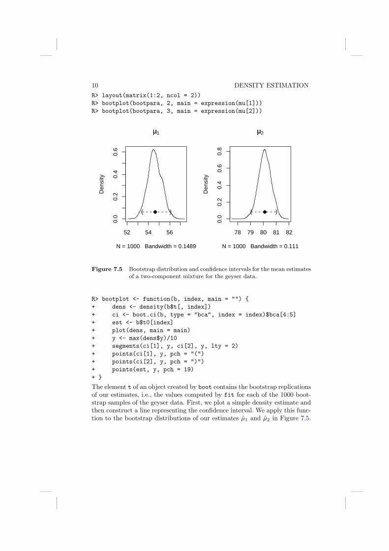
10 DENSITY ESTIMATIONR> layout(matrix(1:2, ncol = 2))R> bootplot(bootpara, 2, main = expression(mu[1]))R> bootplot(bootpara, 3, main = expression(mu[2]))
52 54 56
0.0
0.2
0.4
0.6
µµ1
N = 1000 Bandwidth = 0.1489
Den
sity
( )●
78 79 80 81 82
0.0
0.2
0.4
0.6
0.8
µµ2
N = 1000 Bandwidth = 0.111
Den
sity
( )●
Figure 7.5 Bootstrap distribution and confidence intervals for the mean estimatesof a two-component mixture for the geyser data.
R> bootplot <- function(b, index, main = "") {+ dens <- density(b$t[, index])+ ci <- boot.ci(b, type = "bca", index = index)$bca[4:5]+ est <- b$t0[index]+ plot(dens, main = main)+ y <- max(dens$y)/10+ segments(ci[1], y, ci[2], y, lty = 2)+ points(ci[1], y, pch = "(")+ points(ci[2], y, pch = ")")+ points(est, y, pch = 19)+ }
The element t of an object created by boot contains the bootstrap replicationsof our estimates, i.e., the values computed by fit for each of the 1000 boot-strap samples of the geyser data. First, we plot a simple density estimate andthen construct a line representing the confidence interval. We apply this func-tion to the bootstrap distributions of our estimates µ1 and µ2 in Figure 7.5.

Bibliography
Canty, A. and Ripley, B. D. (2006), boot: Bootstrap R (S-PLUS) Functions(Canty), URL http://CRAN.R-project.org, R package version 1.2-26.
Efron, B. and Tibshirani, R. J. (1993), An Introduction to the Bootstrap,London, UK: Chapman & Hall/CRC.
Fraley, C. and Raftery, A. E. (2002), “Model-based clustering, discriminantanalysis, and density estimation,” Journal of the American Statistical As-sociation, 97, 611–631.
Fraley, C., Raftery, A. E., and Wehrens, R. (2006), mclust: Model-based Clus-ter Analysis, URL http://www.stat.washington.edu/mclust, R packageversion 3.0-0.
Leisch, F. (2004), “FlexMix: A general framework for finite mixture modelsand latent class regression in R,” Journal of Statistical Software, 11, URLhttp://www.jstatsoft.org/v11/i08/.
CHAPTER 8
Recursive Partitioning: LargeCompanies and Glaucoma Diagnosis
8.1 Introduction
8.2 Recursive Partitioning
8.3 Analysis Using R
8.3.1 Forbes 2000 Data
For some observations the profit is missing and we first remove those compa-nies from the list
R> data("Forbes2000", package = "HSAUR")R> Forbes2000 <- subset(Forbes2000, !is.na(profits))
The rpart function from rpart can be used to grow a regression tree. Theresponse variable and the covariates are defined by a model formula in thesame way as for lm, say. By default, a large initial tree is grown.
R> library("rpart")R> forbes_rpart <- rpart(profits ~ assets + marketvalue ++ sales, data = Forbes2000)
A print method for rpart objects is available, however, a graphical represen-tation shown in Figure 8.1 is more convenient. Observations which satisfy thecondition shown for each node go to the left and observations which don’t areelement of the right branch in each node. The numbers plotted in the leavesare the mean profit for those observations satisfying the conditions statedabove. For example, the highest profit is observed for companies with a mar-ket value greater than 89.33 billion US dollars and with more than 91.92 USdollars sales. To determine if the tree is appropriate or if some of the branchesneed to be subjected to pruning we can use the cptable element of the rpartobject:
R> print(forbes_rpart$cptable)
CP nsplit rel error xerror xstd1 0.23748446 0 1.0000000 1.0010339 0.19463312 0.04600397 1 0.7625155 0.8397144 0.21742453 0.04258786 2 0.7165116 0.8066685 0.21663394 0.02030891 3 0.6739237 0.7625940 0.20896845 0.01854336 4 0.6536148 0.7842574 0.20936836 0.01102304 5 0.6350714 0.7925891 0.2106088
3
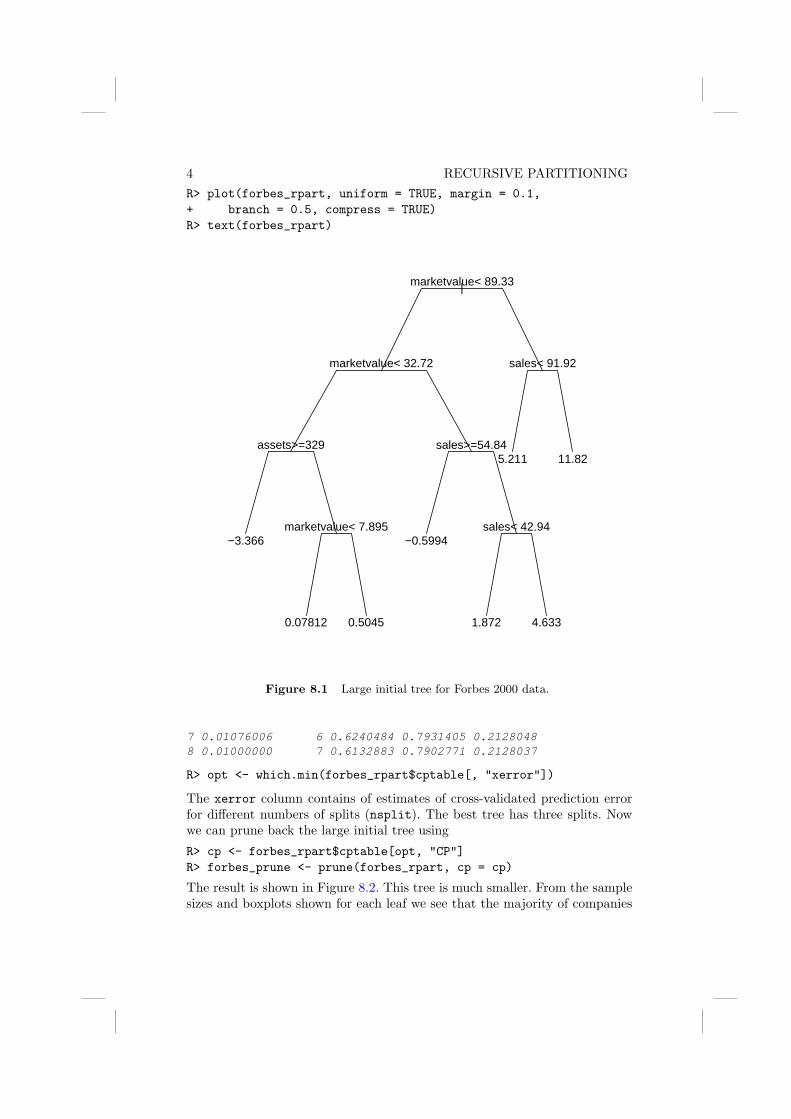
4 RECURSIVE PARTITIONINGR> plot(forbes_rpart, uniform = TRUE, margin = 0.1,+ branch = 0.5, compress = TRUE)R> text(forbes_rpart)
|marketvalue< 89.33
marketvalue< 32.72
assets>=329
marketvalue< 7.895
sales>=54.84
sales< 42.94
sales< 91.92
−3.366
0.07812 0.5045
−0.5994
1.872 4.633
5.211 11.82
Figure 8.1 Large initial tree for Forbes 2000 data.
7 0.01076006 6 0.6240484 0.7931405 0.21280488 0.01000000 7 0.6132883 0.7902771 0.2128037
R> opt <- which.min(forbes_rpart$cptable[, "xerror"])
The xerror column contains of estimates of cross-validated prediction errorfor different numbers of splits (nsplit). The best tree has three splits. Nowwe can prune back the large initial tree using
R> cp <- forbes_rpart$cptable[opt, "CP"]R> forbes_prune <- prune(forbes_rpart, cp = cp)
The result is shown in Figure 8.2. This tree is much smaller. From the samplesizes and boxplots shown for each leaf we see that the majority of companies

ANALYSIS USING R 5
is grouped together. However, a large market value, more that 32.72 billionUS dollars, seems to be a good indicator of large profits.
8.3.2 Glaucoma Diagnosis
R> data("GlaucomaM", package = "ipred")R> glaucoma_rpart <- rpart(Class ~ ., data = GlaucomaM,+ control = rpart.control(xval = 100))R> glaucoma_rpart$cptable
CP nsplit rel error xerror xstd1 0.65306122 0 1.0000000 1.5306122 0.060543912 0.07142857 1 0.3469388 0.3877551 0.056476303 0.01360544 2 0.2755102 0.3775510 0.055904314 0.01000000 5 0.2346939 0.4489796 0.05960655
R> opt <- which.min(glaucoma_rpart$cptable[, "xerror"])R> cp <- glaucoma_rpart$cptable[opt, "CP"]R> glaucoma_prune <- prune(glaucoma_rpart, cp = cp)
As we discussed earlier, the choice of the appropriate sized tree is not a triv-ial problem. For the glaucoma data, the above choice of three leaves is veryunstable across multiple runs of cross-validation. As an illustration of thisproblem we repeat the very same analysis as shown above and record theoptimal number of splits as suggested by the cross-validation runs.R> nsplitopt <- vector(mode = "integer", length = 25)R> for (i in 1:length(nsplitopt)) {+ cp <- rpart(Class ~ ., data = GlaucomaM)$cptable+ nsplitopt[i] <- cp[which.min(cp[, "xerror"]),+ "nsplit"]+ }R> table(nsplitopt)
nsplitopt1 2 514 7 4
Although for 14 runs of cross-validation a simple tree with one split only issuggested, larger trees would have been favored in 11 of the cases. This shortanalysis shows that we should not trust the tree in Figure 8.3 too much. Oneway out of this dilemma is the aggregation of multiple trees via bagging. In R,the bagging idea can be implemented by three or four lines of code. Case countor weight vectors representing the bootstrap samples can be drawn from themultinominal distribution with parameters n and p1 = 1/n, . . . , pn = 1/n viathe rmultinom function. For each weight vector, one large tree is constructedwithout pruning and the rpart objects are stored in a list, here called trees:R> trees <- vector(mode = "list", length = 25)R> n <- nrow(GlaucomaM)R> bootsamples <- rmultinom(length(trees), n, rep(1,

6 RECURSIVE PARTITIONINGR> layout(matrix(1:2, nc = 1))R> plot(forbes_prune, uniform = TRUE, margin = 0.1,+ branch = 0.5, compress = TRUE)R> text(forbes_prune)R> rn <- rownames(forbes_prune$frame)R> lev <- rn[sort(unique(forbes_prune$where))]R> where <- factor(rn[forbes_prune$where], levels = lev)R> n <- tapply(Forbes2000$profits, where, length)R> boxplot(Forbes2000$profits ~ where, varwidth = TRUE,+ ylim = range(Forbes2000$profit) * 1.3, pars = list(axes = FALSE),+ ylab = "Profits in US dollars")R> abline(h = 0, lty = 3)R> axis(2)R> text(1:length(n), max(Forbes2000$profit) * 1.2,+ paste("n = ", n))
|marketvalue< 89.33
marketvalue< 32.72
assets>=329
sales< 91.92
−3.366 0.1964
1.728 5.211 11.82
●
●●●●●●●●
●●●●●●●●●●●●●●●●●●●●●●●●●●●●●●●●●●●●●●●●●●●●●●●●●●●●●●●●●●●●●●●●●●●●
●
●●●●●●●●●●●●●●●●●●●●●●●●●●●●●●●●●●●●●●●●●●●●●●●●●●●●
●
●●●
●
●●●●●●●●●●●●●
●
●●
●
●●
●
●●●●●●●●●●●
●
●
●●●●●●
●
●●●●●●●●●●
●
●●●●●●●●
●●●
●
●●
●●●
●●●●●●●●●
●●●●●●●●●●●●●
●●●●●●●●●●●●●●●●●●●●●●●●●●●●●●●●
●
●
●
●
●
●●●
●
●
−30
−20
−10
010
20
n = 10 n = 1835 n = 117 n = 24 n = 9
Figure 8.2 Pruned regression tree for Forbes 2000 data with the distribution ofthe profit in each leaf depicted by a boxplot.

ANALYSIS USING R 7R> layout(matrix(1:2, nc = 1))R> plot(glaucoma_prune, uniform = TRUE, margin = 0.1,+ branch = 0.5, compress = TRUE)R> text(glaucoma_prune, use.n = TRUE)R> rn <- rownames(glaucoma_prune$frame)R> lev <- rn[sort(unique(glaucoma_prune$where))]R> where <- factor(rn[glaucoma_prune$where], levels = lev)R> mosaicplot(table(where, GlaucomaM$Class), main = "",+ xlab = "", las = 1)
|varg< 0.209
mhcg>=0.1695glaucoma
70/6
glaucoma7/0
normal 21/92
2 6 7
glaucoma
normal
Figure 8.3 Pruned classification tree of the glaucoma data with class distributionin the leaves depicted by a mosaicplot.

8 RECURSIVE PARTITIONING
+ n)/n)R> mod <- rpart(Class ~ ., data = GlaucomaM, control = rpart.control(xval = 0))R> for (i in 1:length(trees)) trees[[i]] <- update(mod,+ weights = bootsamples[, i])
The update function re-evaluates the call of mod, however, with the weightsbeing altered, i.e., fits a tree to a bootstrap sample specified by the weights.It is interesting to have a look at the structures of the multiple trees. Forexample, the variable selected for splitting in the root of the tree is not uniqueas can be seen byR> table(sapply(trees, function(x) as.character(x$frame$var[1])))
phcg varg vari vars1 14 9 1
Although varg is selected most of the time, other variables such as vari oc-cur as well – a further indication that the tree in Figure 8.3 is questionableand that hard decisions are not appropriate for the glaucoma data. In orderto make use of the ensemble of trees in the list trees we estimate the con-ditional probability of suffering from glaucoma given the covariates for eachobservation in the original data set byR> classprob <- matrix(0, nrow = n, ncol = length(trees))R> for (i in 1:length(trees)) {+ classprob[, i] <- predict(trees[[i]], newdata = GlaucomaM)[,+ 2]+ classprob[bootsamples[, i] > 0, i] <- NA+ }
Thus, for each observation we get 25 estimates. However, each observation hasbeen used for growing one of the trees with probability 0.632 and thus was notused with probability 0.368. Consequently, the estimate from a tree where anobservation was not used for growing is better for judging the quality of thepredictions and we label the other estimates with NA. Now, we can average theestimates and we vote for glaucoma when the average of the estimates of theconditional glaucoma probability exceeds 0.5. The comparison between theobserved and the predicted classes does not suffer from overfitting since thepredictions are computed from those trees for which each single observationwas not used for growing.R> avg <- rowMeans(classprob, na.rm = TRUE)R> predictions <- factor(avg > 0.5, labels = levels(GlaucomaM$Class))R> predtab <- table(predictions, GlaucomaM$Class)R> predtab
predictions glaucoma normalglaucoma 78 15normal 20 83
Thus, an honest estimate of the probability of a glaucoma prediction whenthe patient is actually suffering from glaucoma is

ANALYSIS USING R 9
R> round(predtab[1, 1]/colSums(predtab)[1] * 100)
glaucoma80
per cent. ForR> round(predtab[2, 2]/colSums(predtab)[2] * 100)
normal85
per cent of normal eyes, the ensemble does not predict a glaucomateous dam-age. The bagging procedure is a special case of a more general approach calledrandom forest (Breiman, 2001). The package randomForest (Breiman et al.,2006) can be used to compute such ensembles viaR> library("randomForest")R> rf <- randomForest(Class ~ ., data = GlaucomaM)
and we obtain out-of-bag estimates for the prediction error viaR> table(predict(rf), GlaucomaM$Class)
glaucoma normalglaucoma 81 11normal 17 87
For the glaucoma data, such a conditional inference tree can be computedusing the ctree functionR> library("party")R> glaucoma_ctree <- ctree(Class ~ ., data = GlaucomaM)
and a graphical representation is depicted in Figure 8.5 showing both thecutpoints and the p-values of the associated independence tests for each node.The first split is performed using a cutpoint defined with respect to the volumeof the optic nerve above some reference plane, but in the inferior part of theeye only (vari).

10 RECURSIVE PARTITIONINGR> library("lattice")R> gdata <- data.frame(avg = rep(avg, 2), class = rep(as.numeric(GlaucomaM$Class),+ 2), obs = c(GlaucomaM[["varg"]], GlaucomaM[["vari"]]),+ var = factor(c(rep("varg", nrow(GlaucomaM)),+ rep("vari", nrow(GlaucomaM)))))R> panelf <- function(x, y) {+ panel.xyplot(x, y, pch = gdata$class)+ panel.abline(h = 0.5, lty = 2)+ }R> print(xyplot(avg ~ obs | var, data = gdata, panel = panelf,+ scales = "free", xlab = "", ylab = "Estimated Class Probability Glaucoma"))
Est
imat
ed C
lass
Pro
babi
lity
Gla
ucom
a0.
00.
20.
40.
60.
81.
0
0.0 0.5 1.0
●
●
●●
●
●
●
●
●
●
●
●
●
●
●●●
●●
●
●
●
●
●●
●
●●
●
●
●
●
●
●
●
●
●
●●
●
● ●
● ●●●
●
●
●
●●
●
●
●
●
●
●●
●
●
●
●
●●
●
●
●
●
●
●●●● ●
●
● ●●
●
●
●
●
● ●
●
●
●●
●
●
●
●
●
●
●
●
●
●
varg
0.0
0.2
0.4
0.6
0.8
1.0
0.00 0.05 0.10 0.15 0.20 0.25
●
●
●●
●
●
●
●
●
●
●
●
●
●
●●●
●●
●
●
●
●
●●
●
●●
●
●
●
●
●
●
●
●
●
●●
●
● ●
● ●●●
●
●
●
●●
●
●
●
●
●
●●
●
●
●
●
●●
●
●
●
●
●
●● ●● ●
●
●● ●
●
●
●
●
● ●
●
●
●●
●
●
●
●
●
●
●
●
●
●
vari
Figure 8.4 Glaucoma data: Estimated class probabilities depending on two im-portant variables. The 0.5 cut-off for the estimated glaucoma proba-bility is depicted as horizontal line. Glaucomateous eyes are plottedas circles and normal eyes are triangles.
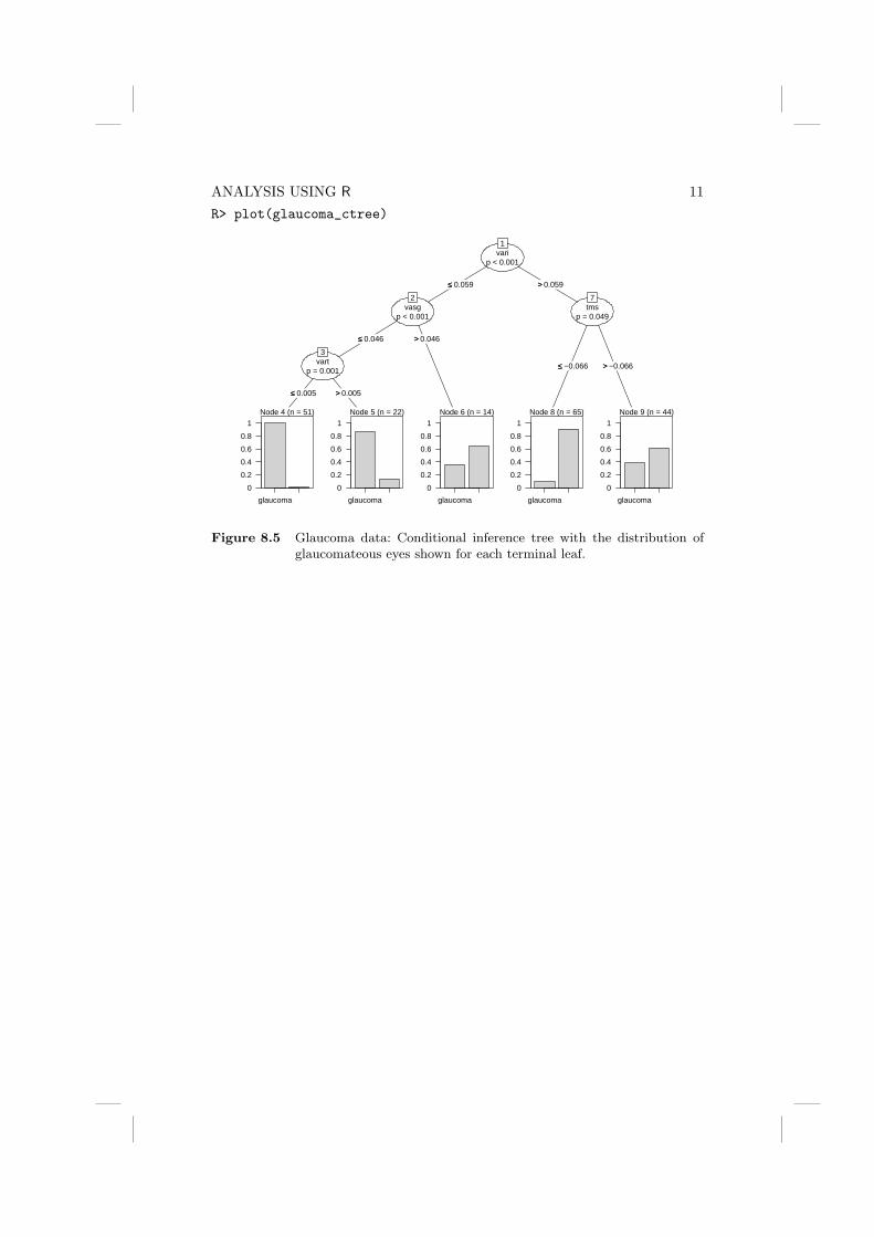
ANALYSIS USING R 11R> plot(glaucoma_ctree)
varip < 0.001
1
≤≤ 0.059 >> 0.059
vasgp < 0.001
2
≤≤ 0.046 >> 0.046
vartp = 0.001
3
≤≤ 0.005 >> 0.005
Node 4 (n = 51)
glaucoma
0
0.2
0.4
0.6
0.8
1Node 5 (n = 22)
glaucoma
0
0.2
0.4
0.6
0.8
1Node 6 (n = 14)
glaucoma
0
0.2
0.4
0.6
0.8
1
tmsp = 0.049
7
≤≤ −0.066 >> −0.066
Node 8 (n = 65)
glaucoma
0
0.2
0.4
0.6
0.8
1Node 9 (n = 44)
glaucoma
0
0.2
0.4
0.6
0.8
1
Figure 8.5 Glaucoma data: Conditional inference tree with the distribution ofglaucomateous eyes shown for each terminal leaf.


Bibliography
Breiman, L. (2001), “Random forests,” Machine Learning , 45, 5–32.Breiman, L., Cutler, A., Liaw, A., and Wiener, M. (2006), randomForest:
Breiman and Cutler’s Random Forests for Classification and Regression,URL http://stat-www.berkeley.edu/users/breiman/RandomForests,R package version 4.5-16.

CHAPTER 9
Survival Analysis:Glioma Treatment and Breast Cancer
Survival
9.1 Introduction
9.2 Survival Analysis
9.3 Analysis Using R
9.3.1 Glioma Radioimmunotherapy
Figure 9.1 leads to the impression that patients treated with the novel ra-dioimmunotherapy survive longer, regardless of the tumor type. In order toassess if this informal finding is reliable, we may perform a log-rank test via
R> survdiff(Surv(time, event) ~ group, data = g3)
Call:survdiff(formula = Surv(time, event) ~ group, data = g3)
N Observed Expected (O-E)^2/E (O-E)^2/Vgroup=Control 6 4 1.49 4.23 6.06group=RIT 11 2 4.51 1.40 6.06
Chisq= 6.1 on 1 degrees of freedom, p= 0.0138
which indicates that the survival times are indeed different in both groups.However, the number of patients is rather limited and so it might be danger-ous to rely on asymptotic tests. As shown in Chapter 3, conditioning on thedata and computing the distribution of the test statistics without additionalassumptions is one alternative. The function surv_test from package coin(Hothorn et al., 2006b,a) can be used to compute an exact conditional testanswering the question whether the survival times differ for grade III patients:
R> library("coin")R> surv_test(Surv(time, event) ~ group, data = g3,+ distribution = "exact")
Exact Logrank Test
data: Surv(time, event) by groups Control, RITZ = 2.1711, p-value = 0.02877alternative hypothesis: two.sided
3
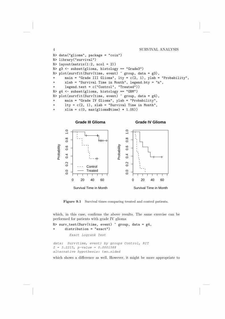
4 SURVIVAL ANALYSISR> data("glioma", package = "coin")R> library("survival")R> layout(matrix(1:2, ncol = 2))R> g3 <- subset(glioma, histology == "Grade3")R> plot(survfit(Surv(time, event) ~ group, data = g3),+ main = "Grade III Glioma", lty = c(2, 1), ylab = "Probability",+ xlab = "Survival Time in Month", legend.bty = "n",+ legend.text = c("Control", "Treated"))R> g4 <- subset(glioma, histology == "GBM")R> plot(survfit(Surv(time, event) ~ group, data = g4),+ main = "Grade IV Glioma", ylab = "Probability",+ lty = c(2, 1), xlab = "Survival Time in Month",+ xlim = c(0, max(glioma$time) * 1.05))
0 20 40 60
0.0
0.2
0.4
0.6
0.8
1.0
Grade III Glioma
Survival Time in Month
Pro
babi
lity
ControlTreated
0 20 40 60
0.0
0.2
0.4
0.6
0.8
1.0
Grade IV Glioma
Survival Time in Month
Pro
babi
lity
Figure 9.1 Survival times comparing treated and control patients.
which, in this case, confirms the above results. The same exercise can beperformed for patients with grade IV gliomaR> surv_test(Surv(time, event) ~ group, data = g4,+ distribution = "exact")
Exact Logrank Test
data: Surv(time, event) by groups Control, RITZ = 3.2215, p-value = 0.0001588alternative hypothesis: two.sided
which shows a difference as well. However, it might be more appropriate to

ANALYSIS USING R 5
answer the question whether the novel therapy is superior for both groups oftumors simultaneously. This can be implemented by stratifying, or blocking,with respect tumor grading:
R> surv_test(Surv(time, event) ~ group | histology,+ data = glioma, distribution = approximate(B = 10000))
Approximative Logrank Test
data: Surv(time, event) bygroups Control, RITstratified by histology
Z = 3.6704, p-value = 1e-04alternative hypothesis: two.sided
Here, we need to approximate the exact conditional distribution since the exactdistribution is hard to compute. The result supports the initial impressionimplied by Figure 9.1
9.3.2 Breast Cancer Survival
Before fitting a Cox model to the GBSG2 data, we again derive a Kaplan-Meierestimate of the survival function of the data, here stratified with respect towhether a patient received a hormonal therapy or not (see Figure 9.2). Fittinga Cox model follows roughly the same rules are shown for linear models inChapters 4, 5 or 6 with the exception that the response variable is again codedas a Surv object. For the GBSG2 data, the model is fitted via
R> GBSG2_coxph <- coxph(Surv(time, cens) ~ ., data = GBSG2)
and the results as given by the summary method are given in Figure 9.3. Sincewe are especially interested in the relative risk for patients who underwenta hormonal therapy, we can compute an estimate of the relative risk and acorresponding confidence interval via
R> ci <- confint(GBSG2_coxph)R> exp(cbind(coef(GBSG2_coxph), ci))["horThyes", ]
2.5 % 97.5 %0.7073155 0.5492178 0.9109233
This result implies that patients treated with a hormonal therapy had a lowerrisk and thus survived longer compared to women who were not treated thisway. Model checking and model selection for proportional hazardsmodels are complicated by the fact that easy to use residuals, such as thosediscussed in Chapter 5 for linear regression model are not available, but severalpossibilities do exist. A check of the proportional hazards assumption can bedone by looking at the parameter estimates β1, . . . , βq over time. We can safelyassume proportional hazards when the estimates don’t vary much over time.The null hypothesis of constant regression coefficients can be tested, bothglobally as well as for each covariate, by using the cox.zph function

6 SURVIVAL ANALYSISR> data("GBSG2", package = "ipred")R> plot(survfit(Surv(time, cens) ~ horTh, data = GBSG2),+ lty = 1:2, mark.time = FALSE, ylab = "Probability",+ xlab = "Survival Time in Days")R> legend(250, 0.2, legend = c("yes", "no"), lty = c(2,+ 1), title = "Hormonal Therapy", bty = "n")
0 500 1000 1500 2000 2500
0.0
0.2
0.4
0.6
0.8
1.0
Survival Time in Days
Pro
babi
lity
Hormonal Therapy
yesno
Figure 9.2 Kaplan-Meier estimates for breast cancer patients who either receiveda hormonal therapy or not.
R> GBSG2_zph <- cox.zph(GBSG2_coxph)R> GBSG2_zph
rho chisq phorThyes -2.54e-02 1.96e-01 0.65778age 9.40e-02 2.96e+00 0.08552menostatPost -1.19e-05 3.75e-08 0.99985tsize -2.50e-02 1.88e-01 0.66436tgrade.L -1.30e-01 4.85e+00 0.02772

ANALYSIS USING R 7
R> summary(GBSG2_coxph)
Call:coxph(formula = Surv(time, cens) ~ ., data = GBSG2)
n= 686coef exp(coef) se(coef) z p
horThyes -0.346278 0.707 0.129075 -2.683 7.3e-03age -0.009459 0.991 0.009301 -1.017 3.1e-01menostatPost 0.258445 1.295 0.183476 1.409 1.6e-01tsize 0.007796 1.008 0.003939 1.979 4.8e-02tgrade.L 0.551299 1.736 0.189844 2.904 3.7e-03tgrade.Q -0.201091 0.818 0.121965 -1.649 9.9e-02pnodes 0.048789 1.050 0.007447 6.551 5.7e-11progrec -0.002217 0.998 0.000574 -3.866 1.1e-04estrec 0.000197 1.000 0.000450 0.438 6.6e-01
exp(coef) exp(-coef) lower .95 upper .95horThyes 0.707 1.414 0.549 0.911age 0.991 1.010 0.973 1.009menostatPost 1.295 0.772 0.904 1.855tsize 1.008 0.992 1.000 1.016tgrade.L 1.736 0.576 1.196 2.518tgrade.Q 0.818 1.223 0.644 1.039pnodes 1.050 0.952 1.035 1.065progrec 0.998 1.002 0.997 0.999estrec 1.000 1.000 0.999 1.001
Rsquare= 0.142 (max possible= 0.995 )Likelihood ratio test= 105 on 9 df, p=0Wald test = 115 on 9 df, p=0Score (logrank) test = 121 on 9 df, p=0
Figure 9.3 R output of the summary method for GBSG2_coxph.
tgrade.Q 3.22e-03 3.14e-03 0.95530pnodes 5.84e-02 5.98e-01 0.43941progrec 5.65e-02 1.20e+00 0.27351estrec 5.46e-02 1.03e+00 0.30967GLOBAL NA 2.27e+01 0.00695
There seems to be some evidence of time-varying effects, especially for ageand tumor grading. A graphical representation of the estimated regression co-efficient over time is shown in Figure 9.4. We refer to Therneau and Gramb-sch (2000) for a detailed theoretical description of these topics. The tree-structured regression models applied to continuous and binary responses inChapter 8 are applicable to censored responses in survival analysis as well.Such a simple prognostic model with only a few terminal nodes might be
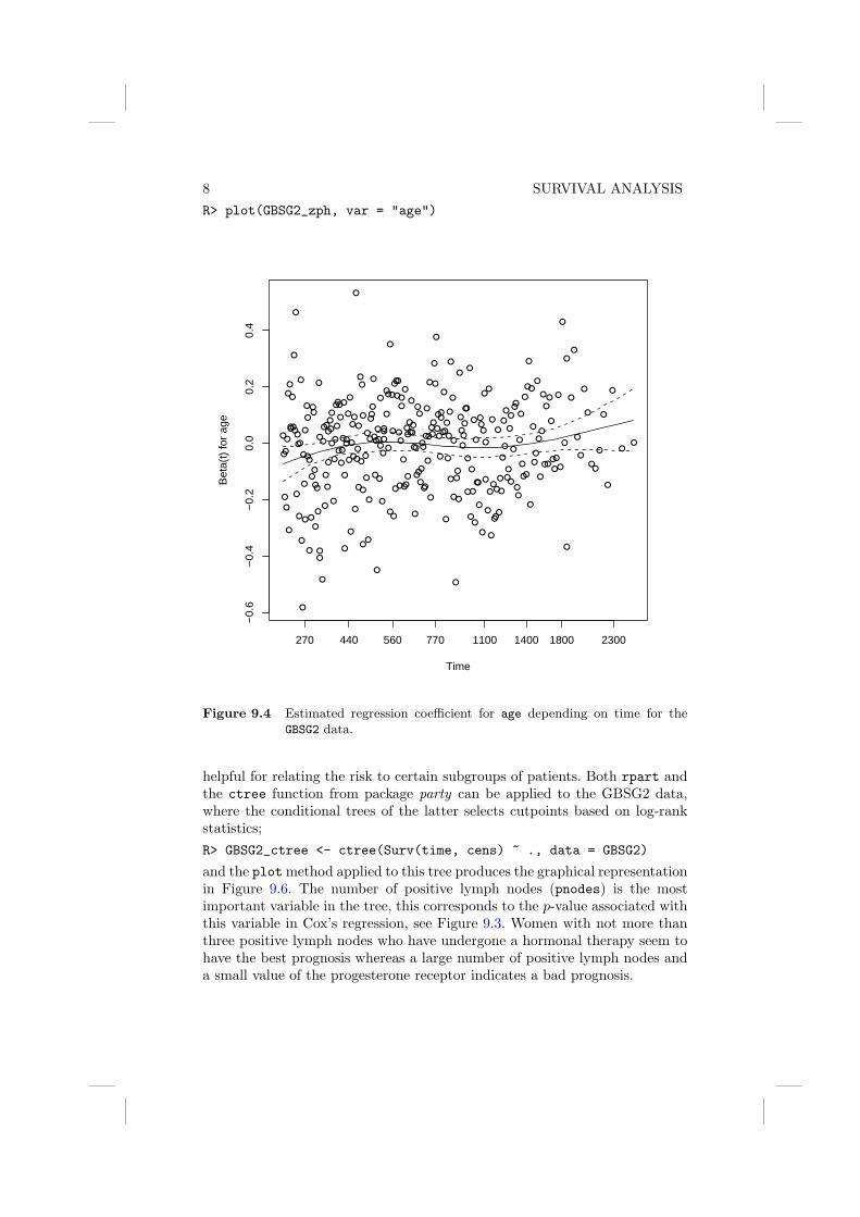
8 SURVIVAL ANALYSISR> plot(GBSG2_zph, var = "age")
Time
Bet
a(t)
for
age
270 440 560 770 1100 1400 1800 2300
−0.
6−
0.4
−0.
20.
00.
20.
4
●
●
●
●
●
●
●
●
●
●●
●
●
●
●
●
●
●
●
●
●
●
●
●
●
●
●
●
●
●
●
●
●
●
●
●●
●
●
●
●
●
●
●
●●
●
●
●
●
●
●
●
●
●
●
●
●
●
●
●
●
●
●
●
●
●
●
●
●
●
●
●
●
●●
●
●
●
●
●
●
●
●
●
●
●
●
●
●
●
●
●
●
●
●
●
●
●
●
●
●
●●●
●
●
●
●
●
●
●
●
●
●
●
●
●●●
●
●●
●
●
●
●
●
●
●
●
●
●
●
●
●
●
●
●
●
●
●
●
●●
●
●
●
●
●●
●
●
●
●
●
●
●
●
●
●●
●●
●
●
●
●
●
●
●●
●
●
●
●
●
●
●
●
●●
●
●
●
●
●
●
●
●
●
●
●
●
●
●
●●
●
●
●
●
●
●
●
●●
●
●
●
●
●
●
●
●
●
●●
●
●●
●
●
●
●
●
●
●
●
●
●
●
●●
●
●
●
●
●
●
●
●
●
●●
●
●
●
●
●●
●●
●
●
●
●
●
●
●
●
●
●
●
●
●
●
●
●
●
●
●
●
●
●
●
●
●
●
●
●
●
●
●
●
●
●
●
●
●
●
●●
●
●
●
●
●●
Figure 9.4 Estimated regression coefficient for age depending on time for theGBSG2 data.
helpful for relating the risk to certain subgroups of patients. Both rpart andthe ctree function from package party can be applied to the GBSG2 data,where the conditional trees of the latter selects cutpoints based on log-rankstatistics;R> GBSG2_ctree <- ctree(Surv(time, cens) ~ ., data = GBSG2)
and the plot method applied to this tree produces the graphical representationin Figure 9.6. The number of positive lymph nodes (pnodes) is the mostimportant variable in the tree, this corresponds to the p-value associated withthis variable in Cox’s regression, see Figure 9.3. Women with not more thanthree positive lymph nodes who have undergone a hormonal therapy seem tohave the best prognosis whereas a large number of positive lymph nodes anda small value of the progesterone receptor indicates a bad prognosis.
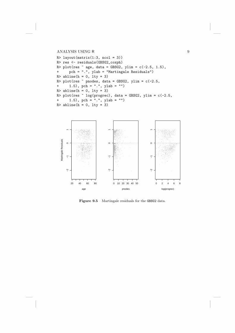
ANALYSIS USING R 9R> layout(matrix(1:3, ncol = 3))R> res <- residuals(GBSG2_coxph)R> plot(res ~ age, data = GBSG2, ylim = c(-2.5, 1.5),+ pch = ".", ylab = "Martingale Residuals")R> abline(h = 0, lty = 3)R> plot(res ~ pnodes, data = GBSG2, ylim = c(-2.5,+ 1.5), pch = ".", ylab = "")R> abline(h = 0, lty = 3)R> plot(res ~ log(progrec), data = GBSG2, ylim = c(-2.5,+ 1.5), pch = ".", ylab = "")R> abline(h = 0, lty = 3)
20 40 60 80
−2
−1
01
age
Mar
tinga
le R
esid
uals
0 10 20 30 40 50
−2
−1
01
pnodes
0 2 4 6 8
−2
−1
01
log(progrec)
Figure 9.5 Martingale residuals for the GBSG2 data.

10 SURVIVAL ANALYSISR> plot(GBSG2_ctree)
pnodesp < 0.001
1
≤≤ 3 >> 3
horThp = 0.035
2
no yes
Node 3 (n = 248)
0 500 1500 2500
0
0.2
0.4
0.6
0.8
1Node 4 (n = 128)
0 500 1500 2500
0
0.2
0.4
0.6
0.8
1
progrecp < 0.001
5
≤≤ 20 >> 20
Node 6 (n = 144)
0 500 1500 2500
0
0.2
0.4
0.6
0.8
1Node 7 (n = 166)
0 500 1500 2500
0
0.2
0.4
0.6
0.8
1
Figure 9.6 GBSG2 data: Conditonal inference tree with the survival function, es-timated by Kaplan-Meier, shown for every subgroup of patients iden-tified by the tree.

Bibliography
Hothorn, T., Hornik, K., van de Wiel, M., and Zeileis, A. (2006a), coin:Conditional Inference Procedures in a Permutation Test Framework , URLhttp://CRAN.R-project.org, R package version 0.4-14.
Hothorn, T., Hornik, K., van de Wiel, M. A., and Zeileis, A. (2006b),“A Lego system for conditional inference,” The American Statistician,60, 257–263, URL http://statmath.wu-wien.ac.at/~zeileis/papers/Hothorn+Hornik+VanDeWiel-2006.pdf.
Therneau, T. M. and Grambsch, P. M. (2000), Modeling Survival Data: Ex-tending the Cox Model , New York, USA: Springer.

CHAPTER 10
Analysing Longitudinal Data I:Computerised Delivery of Cognitive
Behavioural Therapy–Beat the Blues
10.1 Introduction
10.2 Analysing Longitudinal Data
10.3 Analysis Using R
We shall fit both random intercept and random intercept and slope modelsto the data including the baseline BDI values (pre.bdi), treatment group,drug and length as fixed effect covariates. Linear mixed effects models arefitted in R by using the lmer function contained in the lme4 package (Batesand Sarkar, 2006, Pinheiro and Bates, 2000, Bates, 2005), but an essentialfirst step is to rearrange the data from the ‘wide form’ in which they appearin the BtheB data frame into the ‘long form’ in which each separate repeatedmeasurement and associated covariate values appear as a separate row in adata.frame. This rearrangement can be made using the following code:R> data("BtheB", package = "HSAUR")R> BtheB$subject <- factor(rownames(BtheB))R> nobs <- nrow(BtheB)R> BtheB_long <- reshape(BtheB, idvar = "subject",+ varying = c("bdi.2m", "bdi.4m", "bdi.6m", "bdi.8m"),+ direction = "long")R> BtheB_long$time <- rep(c(2, 4, 6, 8), rep(nobs,+ 4))
such that the data are now in the form (here shown for the first three subjects)R> subset(BtheB_long, subject %in% c("1", "2", "3"))
drug length treatment bdi.pre subject time bdi1.2m No >6m TAU 29 1 2 22.2m Yes >6m BtheB 32 2 2 163.2m Yes <6m TAU 25 3 2 201.4m No >6m TAU 29 1 4 22.4m Yes >6m BtheB 32 2 4 243.4m Yes <6m TAU 25 3 4 NA1.6m No >6m TAU 29 1 6 NA2.6m Yes >6m BtheB 32 2 6 173.6m Yes <6m TAU 25 3 6 NA
3

4 ANALYSING LONGITUDINAL DATA IR> data("BtheB", package = "HSAUR")R> layout(matrix(1:2, nrow = 1))R> ylim <- range(BtheB[, grep("bdi", names(BtheB))],+ na.rm = TRUE)R> boxplot(subset(BtheB, treatment == "TAU")[, grep("bdi",+ names(BtheB))], main = "Treated as usual", ylab = "BDI",+ xlab = "Time (in months)", names = c(0, 2, 4,+ 6, 8), ylim = ylim)R> boxplot(subset(BtheB, treatment == "BtheB")[, grep("bdi",+ names(BtheB))], main = "Beat the Blues", ylab = "BDI",+ xlab = "Time (in months)", names = c(0, 2, 4,+ 6, 8), ylim = ylim)
0 2 4 6 8
010
2030
4050
Treated as usual
Time (in months)
BD
I
●
●●
0 2 4 6 8
010
2030
4050
Beat the Blues
Time (in months)
BD
I
Figure 10.1 Boxplots for the repeated measures by treatment group for the BtheBdata.
1.8m No >6m TAU 29 1 8 NA2.8m Yes >6m BtheB 32 2 8 203.8m Yes <6m TAU 25 3 8 NA
The resulting data.frame BtheB_long contains a number of missing valuesand in applying the lmer function these will be dropped. But notice it is onlythe missing values that are removed, not participants that have at least onemissing value. All the available data is used in the model fitting process. Thelmer function is used in a similar way to the lm function met in Chapter ??with the addition of a random term to identify the source of the repeated

ANALYSIS USING R 5
measurements, here subject. We can fit the two models (??) and (??) andtest which is most appropriate usingR> library("lme4")R> BtheB_lmer1 <- lmer(bdi ~ bdi.pre + time + treatment ++ drug + length + (1 | subject), data = BtheB_long,+ method = "ML", na.action = na.omit)R> BtheB_lmer2 <- lmer(bdi ~ bdi.pre + time + treatment ++ drug + length + (time | subject), data = BtheB_long,+ method = "ML", na.action = na.omit)R> anova(BtheB_lmer1, BtheB_lmer2)
Data: BtheB_longModels:BtheB_lmer1: bdi ~ bdi.pre + time + treatment + drug + length + (1 | subject)BtheB_lmer2: bdi ~ bdi.pre + time + treatment + drug + length + (time | subject)
Df AIC BIC logLik Chisq Chi DfBtheB_lmer1 7 1884.62 1910.07 -935.31BtheB_lmer2 9 1887.81 1920.52 -934.90 0.8161 2
Pr(>Chisq)BtheB_lmer1BtheB_lmer2 0.665
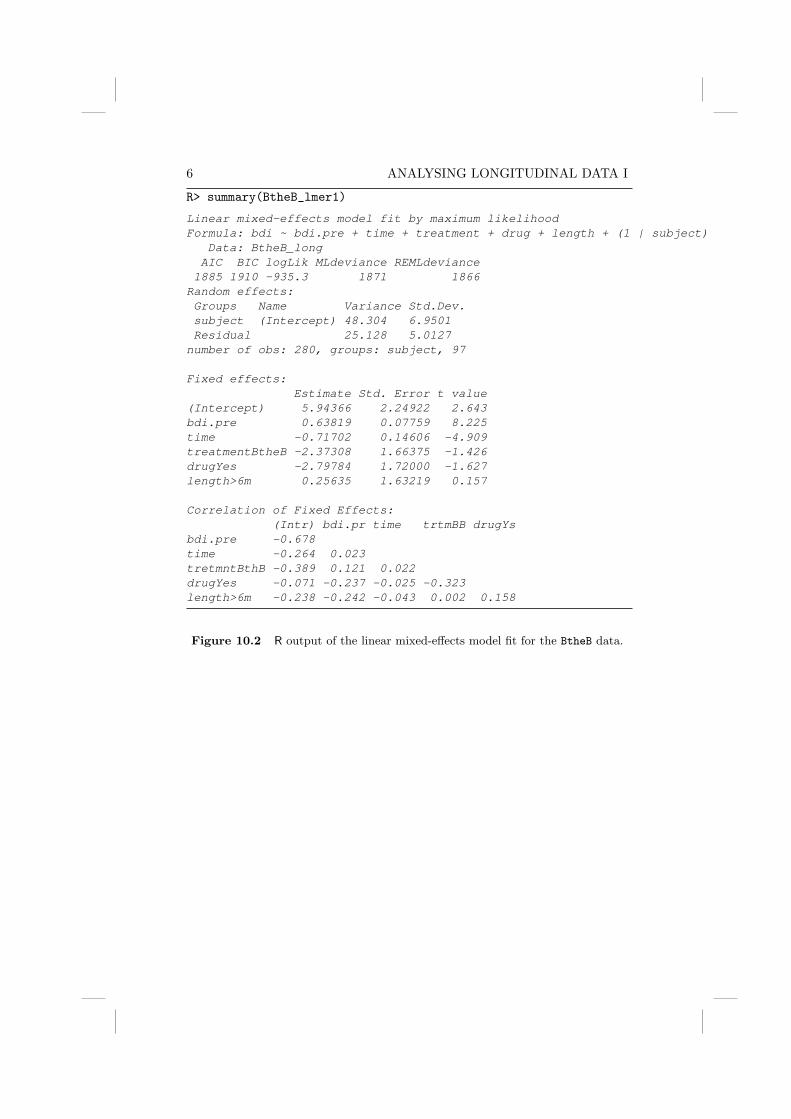
6 ANALYSING LONGITUDINAL DATA I
R> summary(BtheB_lmer1)
Linear mixed-effects model fit by maximum likelihoodFormula: bdi ~ bdi.pre + time + treatment + drug + length + (1 | subject)
Data: BtheB_longAIC BIC logLik MLdeviance REMLdeviance1885 1910 -935.3 1871 1866
Random effects:Groups Name Variance Std.Dev.subject (Intercept) 48.304 6.9501Residual 25.128 5.0127number of obs: 280, groups: subject, 97
Fixed effects:Estimate Std. Error t value
(Intercept) 5.94366 2.24922 2.643bdi.pre 0.63819 0.07759 8.225time -0.71702 0.14606 -4.909treatmentBtheB -2.37308 1.66375 -1.426drugYes -2.79784 1.72000 -1.627length>6m 0.25635 1.63219 0.157
Correlation of Fixed Effects:(Intr) bdi.pr time trtmBB drugYs
bdi.pre -0.678time -0.264 0.023tretmntBthB -0.389 0.121 0.022drugYes -0.071 -0.237 -0.025 -0.323length>6m -0.238 -0.242 -0.043 0.002 0.158
Figure 10.2 R output of the linear mixed-effects model fit for the BtheB data.

Bibliography
Bates, D. (2005), “Fitting linear mixed models in R,” R News, 5, 27–30, URLhttp://CRAN.R-project.org/doc/Rnews/.
Bates, D. and Sarkar, D. (2006), lme4: Linear Mixed-Effects Models Using S4Classes, URL http://CRAN.R-project.org, R package version 0.9975-1.
Pinheiro, J. C. and Bates, D. M. (2000), Mixed-Effects Models in S and S-PLUS , New York, USA: Springer.

CHAPTER 11
Analysing Longitudinal Data II –Generalised Estimation Equations:Treating Respiratory Illness and
Epileptic Seizures
11.1 Introduction
11.2 Generalised Estimating Equations
11.3 Analysis Using R
11.3.1 Beat the Blues Revisited
To use the gee function, package gee (Carey et al., 2006) has to be installedand attached:
R> library("gee")
The gee function is used in a similar way to the lme function met in Chapter10, with the addition of the features of the glm function that specify theappropriate error distribution for the response and the implied link function,and an argument to specify the structure of the working correlation matrix.Here we will fit an independence structure and then an exchangeable structure.The R code for fitting generalised estimation equations to the BtheB_longdata (as constructed in Chapter 10, with idenity working correlation matrixis as follows (note that the gee function assumes the rows of the data.frameBtheB_long to be ordered with respect to subjects)
R> osub <- order(as.integer(BtheB_long$subject))R> BtheB_long <- BtheB_long[osub, ]R> btb_gee <- gee(bdi ~ bdi.pre + treatment + length ++ drug, data = BtheB_long, id = subject, family = gaussian,+ corstr = "independence")
and with exchangeable correlation matrix
R> btb_gee1 <- gee(bdi ~ bdi.pre + treatment + length ++ drug, data = BtheB_long, id = subject, family = gaussian,+ corstr = "exchangeable")
The summary method can be used to inspect the fitted models; the results areshown in Figures 11.1 and 11.2
3

4 ANALYSING LONGITUDINAL DATA II
11.3.2 Respiratory Illness
The baseline status, i.e., the status for month == 0, will enter the models asan explanatory variable and thus we have to rearrange the data.frame res-piratory in order to create a new variable baseline:R> data("respiratory", package = "HSAUR")R> resp <- subset(respiratory, month > "0")R> resp$baseline <- rep(subset(respiratory, month ==+ "0")$status, rep(4, 111))R> resp$nstat <- as.numeric(resp$status == "good")
The new variable nstat is simply a dummy coding for a poor respiratorystatus. Now we can use the data resp to fit a logistic regression model andGEE models with an independent and an exchangeable correlation structureas follows;R> resp_glm <- glm(status ~ centre + treatment + sex ++ baseline + age, data = resp, family = "binomial")R> resp_gee1 <- gee(nstat ~ centre + treatment + sex ++ baseline + age, data = resp, family = "binomial",+ id = subject, corstr = "independence", scale.fix = TRUE,+ scale.value = 1)R> resp_gee2 <- gee(nstat ~ centre + treatment + sex ++ baseline + age, data = resp, family = "binomial",+ id = subject, corstr = "exchangeable", scale.fix = TRUE,+ scale.value = 1)

ANALYSIS USING R 5
R> summary(btb_gee)
GEE: GENERALIZED LINEAR MODELS FOR DEPENDENT DATAgee S-function, version 4.13 modified 98/01/27 (1998)
Model:Link: IdentityVariance to Mean Relation: GaussianCorrelation Structure: Independent
Call:gee(formula = bdi ~ bdi.pre + treatment + length + drug, id = subject,
data = BtheB_long, family = gaussian, corstr = "independence")
Summary of Residuals:Min 1Q Median 3Q Max
-21.6497810 -5.8485100 0.1131663 5.5838383 28.1871039
Coefficients:Estimate Naive S.E. Naive z Robust S.E.
(Intercept) 3.5686314 1.4833349 2.405816 2.26947617bdi.pre 0.5818494 0.0563904 10.318235 0.09156455treatmentBtheB -3.2372285 1.1295569 -2.865928 1.77459534length>6m 1.4577182 1.1380277 1.280916 1.48255866drugYes -3.7412982 1.1766321 -3.179667 1.78271179
Robust z(Intercept) 1.5724472bdi.pre 6.3545274treatmentBtheB -1.8242066length>6m 0.9832449drugYes -2.0986557
Estimated Scale Parameter: 79.25813Number of Iterations: 1
Working Correlation[,1] [,2] [,3] [,4]
[1,] 1 0 0 0[2,] 0 1 0 0[3,] 0 0 1 0[4,] 0 0 0 1
Figure 11.1 R output of the summary method for the btb_gee model.

6 ANALYSING LONGITUDINAL DATA II
R> summary(btb_gee1)
GEE: GENERALIZED LINEAR MODELS FOR DEPENDENT DATAgee S-function, version 4.13 modified 98/01/27 (1998)
Model:Link: IdentityVariance to Mean Relation: GaussianCorrelation Structure: Exchangeable
Call:gee(formula = bdi ~ bdi.pre + treatment + length + drug, id = subject,
data = BtheB_long, family = gaussian, corstr = "exchangeable")
Summary of Residuals:Min 1Q Median 3Q Max
-23.955980 -6.643864 -1.109741 4.257688 25.452310
Coefficients:Estimate Naive S.E. Naive z Robust S.E.
(Intercept) 3.0231602 2.30390185 1.31219140 2.23204410bdi.pre 0.6479276 0.08228567 7.87412417 0.08351405treatmentBtheB -2.1692863 1.76642861 -1.22806339 1.73614385length>6m -0.1112910 1.73091679 -0.06429596 1.55092705drugYes -2.9995608 1.82569913 -1.64296559 1.73155411
Robust z(Intercept) 1.3544357bdi.pre 7.7583066treatmentBtheB -1.2494854length>6m -0.0717577drugYes -1.7322940
Estimated Scale Parameter: 81.7349Number of Iterations: 5
Working Correlation[,1] [,2] [,3] [,4]
[1,] 1.0000000 0.6757951 0.6757951 0.6757951[2,] 0.6757951 1.0000000 0.6757951 0.6757951[3,] 0.6757951 0.6757951 1.0000000 0.6757951[4,] 0.6757951 0.6757951 0.6757951 1.0000000
Figure 11.2 R output of the summary method for the btb_gee1 model.

ANALYSIS USING R 7
R> summary(resp_glm)
Call:glm(formula = status ~ centre + treatment + sex + baseline +
age, family = "binomial", data = resp)
Deviance Residuals:Min 1Q Median 3Q Max
-2.3146 -0.8551 0.4336 0.8953 1.9246
Coefficients:Estimate Std. Error z value Pr(>|z|)
(Intercept) -0.900171 0.337653 -2.666 0.00768 **centre2 0.671601 0.239567 2.803 0.00506 **treatmenttreatment 1.299216 0.236841 5.486 4.12e-08 ***sexmale 0.119244 0.294671 0.405 0.68572baselinegood 1.882029 0.241290 7.800 6.20e-15 ***age -0.018166 0.008864 -2.049 0.04043 *---Signif. codes: 0 '***' 0.001 '**' 0.01 '*' 0.05 '.' 0.1 ' ' 1
(Dispersion parameter for binomial family taken to be 1)
Null deviance: 608.93 on 443 degrees of freedomResidual deviance: 483.22 on 438 degrees of freedomAIC: 495.22
Number of Fisher Scoring iterations: 4
Figure 11.3 R output of the summary method for the resp_glm model.
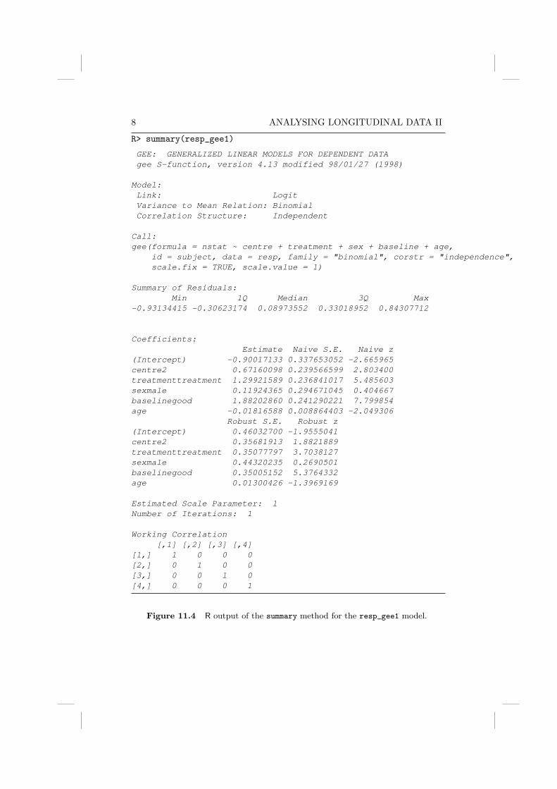
8 ANALYSING LONGITUDINAL DATA II
R> summary(resp_gee1)
GEE: GENERALIZED LINEAR MODELS FOR DEPENDENT DATAgee S-function, version 4.13 modified 98/01/27 (1998)
Model:Link: LogitVariance to Mean Relation: BinomialCorrelation Structure: Independent
Call:gee(formula = nstat ~ centre + treatment + sex + baseline + age,
id = subject, data = resp, family = "binomial", corstr = "independence",scale.fix = TRUE, scale.value = 1)
Summary of Residuals:Min 1Q Median 3Q Max
-0.93134415 -0.30623174 0.08973552 0.33018952 0.84307712
Coefficients:Estimate Naive S.E. Naive z
(Intercept) -0.90017133 0.337653052 -2.665965centre2 0.67160098 0.239566599 2.803400treatmenttreatment 1.29921589 0.236841017 5.485603sexmale 0.11924365 0.294671045 0.404667baselinegood 1.88202860 0.241290221 7.799854age -0.01816588 0.008864403 -2.049306
Robust S.E. Robust z(Intercept) 0.46032700 -1.9555041centre2 0.35681913 1.8821889treatmenttreatment 0.35077797 3.7038127sexmale 0.44320235 0.2690501baselinegood 0.35005152 5.3764332age 0.01300426 -1.3969169
Estimated Scale Parameter: 1Number of Iterations: 1
Working Correlation[,1] [,2] [,3] [,4]
[1,] 1 0 0 0[2,] 0 1 0 0[3,] 0 0 1 0[4,] 0 0 0 1
Figure 11.4 R output of the summary method for the resp_gee1 model.

ANALYSIS USING R 9
R> summary(resp_gee2)
GEE: GENERALIZED LINEAR MODELS FOR DEPENDENT DATAgee S-function, version 4.13 modified 98/01/27 (1998)
Model:Link: LogitVariance to Mean Relation: BinomialCorrelation Structure: Exchangeable
Call:gee(formula = nstat ~ centre + treatment + sex + baseline + age,
id = subject, data = resp, family = "binomial", corstr = "exchangeable",scale.fix = TRUE, scale.value = 1)
Summary of Residuals:Min 1Q Median 3Q Max
-0.93134415 -0.30623174 0.08973552 0.33018952 0.84307712
Coefficients:Estimate Naive S.E. Naive z
(Intercept) -0.90017133 0.47846344 -1.8813796centre2 0.67160098 0.33947230 1.9783676treatmenttreatment 1.29921589 0.33561008 3.8712064sexmale 0.11924365 0.41755678 0.2855747baselinegood 1.88202860 0.34191472 5.5043802age -0.01816588 0.01256110 -1.4462014
Robust S.E. Robust z(Intercept) 0.46032700 -1.9555041centre2 0.35681913 1.8821889treatmenttreatment 0.35077797 3.7038127sexmale 0.44320235 0.2690501baselinegood 0.35005152 5.3764332age 0.01300426 -1.3969169
Estimated Scale Parameter: 1Number of Iterations: 1
Working Correlation[,1] [,2] [,3] [,4]
[1,] 1.0000000 0.3359883 0.3359883 0.3359883[2,] 0.3359883 1.0000000 0.3359883 0.3359883[3,] 0.3359883 0.3359883 1.0000000 0.3359883[4,] 0.3359883 0.3359883 0.3359883 1.0000000
Figure 11.5 R output of the summary method for the resp_gee2 model.

10 ANALYSING LONGITUDINAL DATA II
The estimated treatment effect taken from the exchangeable structure GEEmodel is 1.299 which, using the robust standard errors, has an associated 95%confidence intervalR> se <- summary(resp_gee2)$coefficients["treatmenttreatment",+ "Robust S.E."]R> coef(resp_gee2)["treatmenttreatment"] + c(-1, 1) *+ se * qnorm(0.975)
[1] 0.6117037 1.9867281
These values reflect effects on the log-odds scale. Interpretation becomes sim-pler if we exponentiate the values to get the effects in terms of odds. Thisgives a treatment effect of 3.666 and a 95% confidence interval ofR> exp(coef(resp_gee2)["treatmenttreatment"] + c(-1,+ 1) * se * qnorm(0.975))
[1] 1.843570 7.291637
The odds of achieving a ‘good’ respiratory status with the active treatment isbetween about twice and seven times the corresponding odds for the placebo.
11.3.3 Epilepsy
Moving on to the count data in epilepsy from Table ??, we begin by calcu-lating the means and variances of the number of seizures for all treatment /period interactionsR> data("epilepsy", package = "HSAUR")R> itp <- interaction(epilepsy$treatment, epilepsy$period)R> tapply(epilepsy$seizure.rate, itp, mean)
placebo.1 Progabide.1 placebo.2 Progabide.2 placebo.39.357143 8.580645 8.285714 8.419355 8.785714
Progabide.3 placebo.4 Progabide.48.129032 7.964286 6.709677
R> tapply(epilepsy$seizure.rate, itp, var)
placebo.1 Progabide.1 placebo.2 Progabide.2 placebo.3102.75661 332.71828 66.65608 140.65161 215.28571
Progabide.3 placebo.4 Progabide.4193.04946 58.18386 126.87957
Some of the variances are considerably larger than the corresponding means,which for a Poisson variable may suggest that overdispersion may be a prob-lem, see Chapter ??. We can now fit a Poisson regression model to the dataassuming independence using the glm function. We also use the GEE approachto fit an independence structure, followed by an exchangeable structure usingthe following R code:R> per <- rep(log(2), nrow(epilepsy))R> epilepsy$period <- as.numeric(epilepsy$period)

ANALYSIS USING R 11R> layout(matrix(1:2, nrow = 1))R> ylim <- range(epilepsy$seizure.rate)R> placebo <- subset(epilepsy, treatment == "placebo")R> progabide <- subset(epilepsy, treatment == "Progabide")R> boxplot(seizure.rate ~ period, data = placebo, ylab = "Number of seizures",+ xlab = "Period", ylim = ylim, main = "Placebo")R> boxplot(seizure.rate ~ period, data = progabide,+ main = "Progabide", ylab = "Number of seizures",+ xlab = "Period", ylim = ylim)
●●
●●●
●
●
●●
1 2 3 4
020
4060
8010
0
Placebo
Period
Num
ber
of s
eizu
res
●●
●
● ●●
●
●●●
●
●
●●
●
1 2 3 4
020
4060
8010
0
Progabide
Period
Num
ber
of s
eizu
res
Figure 11.6 Boxplots of numbers of seizures in each two-week period post ran-domisation for placebo and active treatments.
R> epilepsy_glm <- glm(seizure.rate ~ base + age ++ treatment + offset(per), data = epilepsy, family = "poisson")R> epilepsy_gee1 <- gee(seizure.rate ~ base + age ++ treatment + offset(per), data = epilepsy, family = "poisson",+ id = subject, corstr = "independence", scale.fix = TRUE,+ scale.value = 1)R> epilepsy_gee2 <- gee(seizure.rate ~ base + age ++ treatment + offset(per), data = epilepsy, family = "poisson",+ id = subject, corstr = "exchangeable", scale.fix = TRUE,+ scale.value = 1)R> epilepsy_gee3 <- gee(seizure.rate ~ base + age ++ treatment + offset(per), data = epilepsy, family = "poisson",

12 ANALYSING LONGITUDINAL DATA IIR> layout(matrix(1:2, nrow = 1))R> ylim <- range(log(epilepsy$seizure.rate + 1))R> boxplot(log(seizure.rate + 1) ~ period, data = placebo,+ main = "Placebo", ylab = "Log number of seizures",+ xlab = "Period", ylim = ylim)R> boxplot(log(seizure.rate + 1) ~ period, data = progabide,+ main = "Progabide", ylab = "Log number of seizures",+ xlab = "Period", ylim = ylim)
●
1 2 3 4
01
23
4
Placebo
Period
Log
num
ber
of s
eizu
res
●
●
●
●
1 2 3 4
01
23
4
Progabide
Period
Log
num
ber
of s
eizu
res
Figure 11.7 Boxplots of log of numbers of seizures in each two-week period postrandomisation for placebo and active treatments.
+ id = subject, corstr = "exchangeable", scale.fix = FALSE,+ scale.value = 1)
As usual we inspect the fitted models using the summary method, the resultsare given in Figures 11.8, 11.9, 11.10, and 11.11.
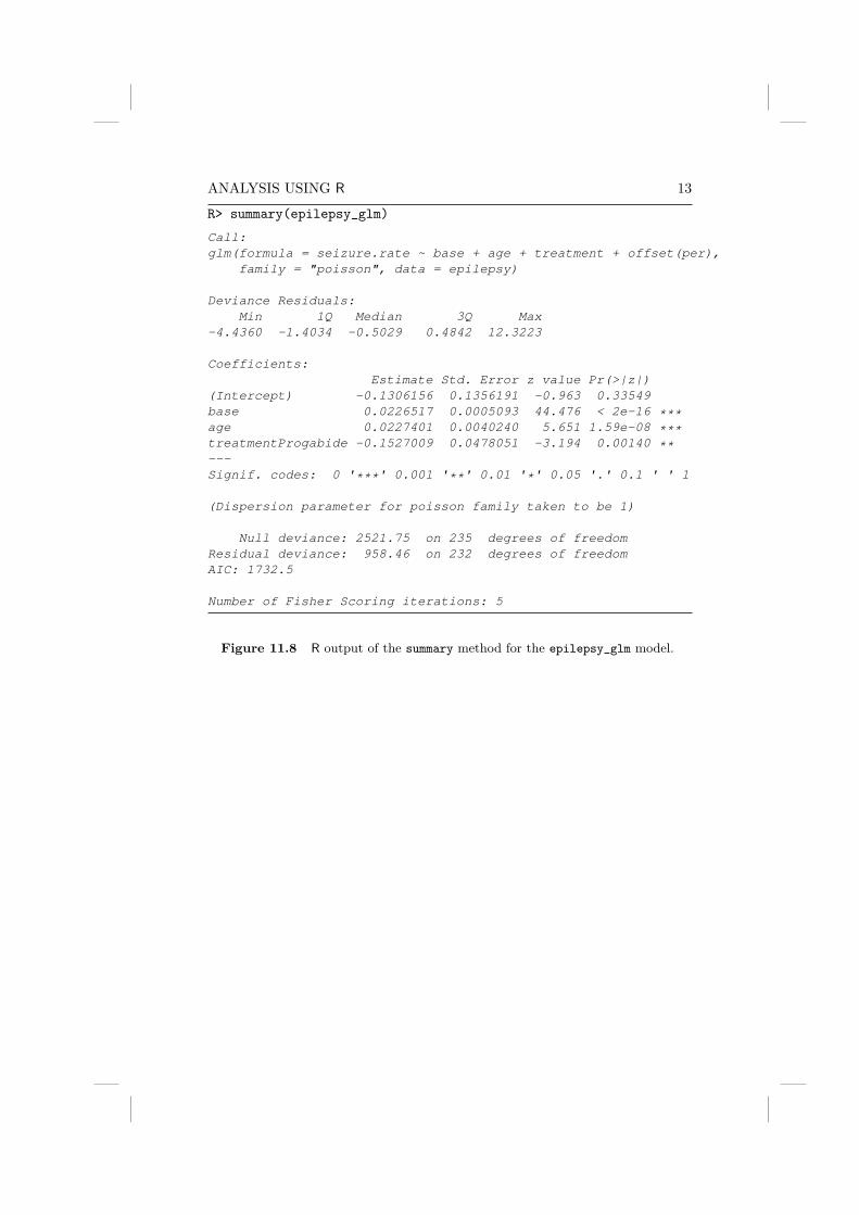
ANALYSIS USING R 13
R> summary(epilepsy_glm)
Call:glm(formula = seizure.rate ~ base + age + treatment + offset(per),
family = "poisson", data = epilepsy)
Deviance Residuals:Min 1Q Median 3Q Max
-4.4360 -1.4034 -0.5029 0.4842 12.3223
Coefficients:Estimate Std. Error z value Pr(>|z|)
(Intercept) -0.1306156 0.1356191 -0.963 0.33549base 0.0226517 0.0005093 44.476 < 2e-16 ***age 0.0227401 0.0040240 5.651 1.59e-08 ***treatmentProgabide -0.1527009 0.0478051 -3.194 0.00140 **---Signif. codes: 0 '***' 0.001 '**' 0.01 '*' 0.05 '.' 0.1 ' ' 1
(Dispersion parameter for poisson family taken to be 1)
Null deviance: 2521.75 on 235 degrees of freedomResidual deviance: 958.46 on 232 degrees of freedomAIC: 1732.5
Number of Fisher Scoring iterations: 5
Figure 11.8 R output of the summary method for the epilepsy_glm model.

14 ANALYSING LONGITUDINAL DATA II
R> summary(epilepsy_gee1)
GEE: GENERALIZED LINEAR MODELS FOR DEPENDENT DATAgee S-function, version 4.13 modified 98/01/27 (1998)
Model:Link: LogarithmVariance to Mean Relation: PoissonCorrelation Structure: Independent
Call:gee(formula = seizure.rate ~ base + age + treatment + offset(per),
id = subject, data = epilepsy, family = "poisson", corstr = "independence",scale.fix = TRUE, scale.value = 1)
Summary of Residuals:Min 1Q Median 3Q Max
-4.9195387 0.1808059 1.7073405 4.8850644 69.9658560
Coefficients:Estimate Naive S.E. Naive z
(Intercept) -0.13061561 0.1356191185 -0.9631062base 0.02265174 0.0005093011 44.4761250age 0.02274013 0.0040239970 5.6511312treatmentProgabide -0.15270095 0.0478051054 -3.1942393
Robust S.E. Robust z(Intercept) 0.365148155 -0.3577058base 0.001235664 18.3316325age 0.011580405 1.9636736treatmentProgabide 0.171108915 -0.8924196
Estimated Scale Parameter: 1Number of Iterations: 1
Working Correlation[,1] [,2] [,3] [,4]
[1,] 1 0 0 0[2,] 0 1 0 0[3,] 0 0 1 0[4,] 0 0 0 1
Figure 11.9 R output of the summary method for the epilepsy_gee1 model.

ANALYSIS USING R 15
R> summary(epilepsy_gee2)
GEE: GENERALIZED LINEAR MODELS FOR DEPENDENT DATAgee S-function, version 4.13 modified 98/01/27 (1998)
Model:Link: LogarithmVariance to Mean Relation: PoissonCorrelation Structure: Exchangeable
Call:gee(formula = seizure.rate ~ base + age + treatment + offset(per),
id = subject, data = epilepsy, family = "poisson", corstr = "exchangeable",scale.fix = TRUE, scale.value = 1)
Summary of Residuals:Min 1Q Median 3Q Max
-4.9195387 0.1808059 1.7073405 4.8850644 69.9658560
Coefficients:Estimate Naive S.E. Naive z
(Intercept) -0.13061561 0.2004416507 -0.651639base 0.02265174 0.0007527342 30.092612age 0.02274013 0.0059473665 3.823564treatmentProgabide -0.15270095 0.0706547450 -2.161227
Robust S.E. Robust z(Intercept) 0.365148155 -0.3577058base 0.001235664 18.3316325age 0.011580405 1.9636736treatmentProgabide 0.171108915 -0.8924196
Estimated Scale Parameter: 1Number of Iterations: 1
Working Correlation[,1] [,2] [,3] [,4]
[1,] 1.0000000 0.3948033 0.3948033 0.3948033[2,] 0.3948033 1.0000000 0.3948033 0.3948033[3,] 0.3948033 0.3948033 1.0000000 0.3948033[4,] 0.3948033 0.3948033 0.3948033 1.0000000
Figure 11.10 R output of the summary method for the epilepsy_gee2 model.

16 ANALYSING LONGITUDINAL DATA II
R> summary(epilepsy_gee3)
GEE: GENERALIZED LINEAR MODELS FOR DEPENDENT DATAgee S-function, version 4.13 modified 98/01/27 (1998)
Model:Link: LogarithmVariance to Mean Relation: PoissonCorrelation Structure: Exchangeable
Call:gee(formula = seizure.rate ~ base + age + treatment + offset(per),
id = subject, data = epilepsy, family = "poisson", corstr = "exchangeable",scale.fix = FALSE, scale.value = 1)
Summary of Residuals:Min 1Q Median 3Q Max
-4.9195387 0.1808059 1.7073405 4.8850644 69.9658560
Coefficients:Estimate Naive S.E. Naive z
(Intercept) -0.13061561 0.452199543 -0.2888451base 0.02265174 0.001698180 13.3388301age 0.02274013 0.013417353 1.6948302treatmentProgabide -0.15270095 0.159398225 -0.9579840
Robust S.E. Robust z(Intercept) 0.365148155 -0.3577058base 0.001235664 18.3316325age 0.011580405 1.9636736treatmentProgabide 0.171108915 -0.8924196
Estimated Scale Parameter: 5.089608Number of Iterations: 1
Working Correlation[,1] [,2] [,3] [,4]
[1,] 1.0000000 0.3948033 0.3948033 0.3948033[2,] 0.3948033 1.0000000 0.3948033 0.3948033[3,] 0.3948033 0.3948033 1.0000000 0.3948033[4,] 0.3948033 0.3948033 0.3948033 1.0000000
Figure 11.11 R output of the summary method for the epilepsy_gee3 model.

Bibliography
Carey, V. J., Lumley, T., and Ripley, B. D. (2006), gee: Generalized EstimationEquation Solver , URL http://CRAN.R-project.org, R package version4.13-11.

CHAPTER 12
Meta-Analysis: Nicotine Gum andSmoking Cessation and the Efficacy of
BCG Vaccine in the Treatment ofTuberculosis
12.1 Introduction
12.2 Systematic Reviews and Meta-Analysis
12.3 Analysis Using R
The aim in collecting the results from the randomised trials of using nicotinegum to help smokers quit was to estimate the overall odds ratio, the odds ofquitting smoking for those given the gum, divided by the odds of quitting forthose not receiving the gum. The odds ratios and corresponding confidenceintervals are computed by means of the meta.MH function for fixed effectsmeta-analysis as shown hereR> library("rmeta")R> data("smoking", package = "HSAUR")R> smokingOR <- meta.MH(smoking[["tt"]], smoking[["tc"]],+ smoking[["qt"]], smoking[["qc"]], names = rownames(smoking))
and the results can be inspected via a summary method – see Figure 12.1.We shall use both the fixed effects and random effects approaches here so
that we can compare results. For the fixed effects model (see Figure 12.1) theestimated overall log-odds ratio is 0.513 with a standard error of 0.066. Thisleads to an estimate of the overall odds ratio of 1.67, with a 95% confidenceinterval as given above. For the random effects modelR> smokingDSL <- meta.DSL(smoking[["tt"]], smoking[["tc"]],+ smoking[["qt"]], smoking[["qc"]], names = rownames(smoking))R> print(smokingDSL)
Random effects ( DerSimonian-Laird ) meta-analysisCall: meta.DSL(ntrt = smoking[["tt"]], nctrl = smoking[["tc"]], ptrt = smoking[["qt"]],
pctrl = smoking[["qc"]], names = rownames(smoking))Summary OR= 1.75 95% CI ( 1.48, 2.07 )Estimated random effects variance: 0.05
the corresponding estimate is 1.751. Both models suggest that there is clearevidence that nicotine gum increases the odds of quitting. The random effectsconfidence interval is considerably wider than that from the fixed effects model;
3

4 META-ANALYSIS
R> summary(smokingOR)
Fixed effects ( Mantel-Haenszel ) meta-analysisCall: meta.MH(ntrt = smoking[["tt"]], nctrl = smoking[["tc"]], ptrt = smoking[["qt"]],
pctrl = smoking[["qc"]], names = rownames(smoking))------------------------------------
OR (lower 95% upper)Blondal89 1.85 0.99 3.46Campbell91 0.98 0.50 1.92Fagerstrom82 1.76 0.80 3.89Fee82 1.53 0.77 3.05Garcia89 2.95 1.01 8.62Garvey00 2.49 1.43 4.34Gross95 2.62 1.03 6.71Hall85 2.03 0.78 5.29Hall87 2.82 1.33 5.99Hall96 0.87 0.46 1.64Hjalmarson84 2.17 1.10 4.28Huber88 6.00 2.57 14.01Jarvis82 3.33 1.37 8.08Jensen91 1.43 0.84 2.44Killen84 1.33 0.43 4.15Killen90 1.23 0.93 1.64Malcolm80 3.52 0.85 14.54McGovern92 1.17 0.70 1.94Nakamura90 3.82 1.15 12.71Niaura94 1.34 0.35 5.19Pirie92 1.84 1.20 2.82Puska79 1.46 0.78 2.75Schneider85 1.71 0.52 5.62Tonnesen88 2.12 0.93 4.86Villa99 1.76 0.55 5.64Zelman92 1.46 0.68 3.14------------------------------------Mantel-Haenszel OR =1.67 95% CI ( 1.47,1.9 )Test for heterogeneity: X^2( 25 ) = 34.9 ( p-value 0.09 )
Figure 12.1 R output of the summary method for smokingOR.
here the test of homogeneity of the studies is not significant implying that wemight use the fixed effects results. But the test is not particularly powerfuland it is more sensible to assume a priori that heterogeneity is present and sowe use the results from the random effects model.

ANALYSIS USING R 5R> plot(smokingOR, ylab = "")
Odds Ratio
0.40 1.00 2.51 6.31 15.85
Blondal89Campbell91Fagerstrom82Fee82Garcia89Garvey00Gross95Hall85Hall87Hall96Hjalmarson84Huber88Jarvis82Jensen91Killen84Killen90Malcolm80McGovern92Nakamura90Niaura94Pirie92Puska79Schneider85Tonnesen88Villa99Zelman92
Summary
Figure 12.2 Forest plot of observed effect sizes and 95% confidence intervals forthe nicotine gum studies.
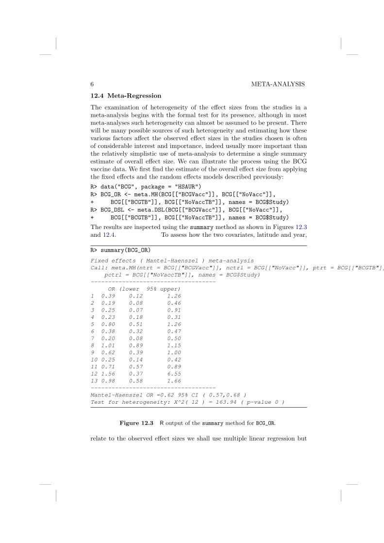
6 META-ANALYSIS
12.4 Meta-Regression
The examination of heterogeneity of the effect sizes from the studies in ameta-analysis begins with the formal test for its presence, although in mostmeta-analyses such heterogeneity can almost be assumed to be present. Therewill be many possible sources of such heterogeneity and estimating how thesevarious factors affect the observed effect sizes in the studies chosen is oftenof considerable interest and importance, indeed usually more important thanthe relatively simplistic use of meta-analysis to determine a single summaryestimate of overall effect size. We can illustrate the process using the BCGvaccine data. We first find the estimate of the overall effect size from applyingthe fixed effects and the random effects models described previously:R> data("BCG", package = "HSAUR")R> BCG_OR <- meta.MH(BCG[["BCGVacc"]], BCG[["NoVacc"]],+ BCG[["BCGTB"]], BCG[["NoVaccTB"]], names = BCG$Study)R> BCG_DSL <- meta.DSL(BCG[["BCGVacc"]], BCG[["NoVacc"]],+ BCG[["BCGTB"]], BCG[["NoVaccTB"]], names = BCG$Study)
The results are inspected using the summary method as shown in Figures 12.3and 12.4. To assess how the two covariates, latitude and year,
R> summary(BCG_OR)
Fixed effects ( Mantel-Haenszel ) meta-analysisCall: meta.MH(ntrt = BCG[["BCGVacc"]], nctrl = BCG[["NoVacc"]], ptrt = BCG[["BCGTB"]],
pctrl = BCG[["NoVaccTB"]], names = BCG$Study)------------------------------------
OR (lower 95% upper)1 0.39 0.12 1.262 0.19 0.08 0.463 0.25 0.07 0.914 0.23 0.18 0.315 0.80 0.51 1.266 0.38 0.32 0.477 0.20 0.08 0.508 1.01 0.89 1.159 0.62 0.39 1.0010 0.25 0.14 0.4211 0.71 0.57 0.8912 1.56 0.37 6.5513 0.98 0.58 1.66------------------------------------Mantel-Haenszel OR =0.62 95% CI ( 0.57,0.68 )Test for heterogeneity: X^2( 12 ) = 163.94 ( p-value 0 )
Figure 12.3 R output of the summary method for BCG_OR.
relate to the observed effect sizes we shall use multiple linear regression but

PUBLICATION BIAS 7
R> summary(BCG_DSL)
Random effects ( DerSimonian-Laird ) meta-analysisCall: meta.DSL(ntrt = BCG[["BCGVacc"]], nctrl = BCG[["NoVacc"]], ptrt = BCG[["BCGTB"]],
pctrl = BCG[["NoVaccTB"]], names = BCG$Study)------------------------------------
OR (lower 95% upper)1 0.39 0.12 1.262 0.19 0.08 0.463 0.25 0.07 0.914 0.23 0.18 0.315 0.80 0.51 1.266 0.38 0.32 0.477 0.20 0.08 0.508 1.01 0.89 1.159 0.62 0.39 1.0010 0.25 0.14 0.4211 0.71 0.57 0.8912 1.56 0.37 6.5513 0.98 0.58 1.66------------------------------------SummaryOR= 0.47 95% CI ( 0.32,0.69 )Test for heterogeneity: X^2( 12 ) = 163.16 ( p-value 0 )Estimated random effects variance: 0.37
Figure 12.4 R output of the summary method for BCG_DSL.
will weight each observation by Wi = (σ2 + V 2i )−1, i = 1, . . . , 13, where σ2 is
the estimated between-study variance and V 2i is the estimated variance from
the ith study. The required R code to fit the linear model via weighted leastsquares is:R> studyweights <- 1/(BCG_DSL$tau2 + BCG_DSL$selogs)R> y <- BCG_DSL$logsR> BCG_mod <- lm(y ~ Latitude + Year, data = BCG, weights = studyweights)
and the results of the summary method are shown in Figure 12.5. There issome evidence that latitude is associated with observed effect size, the log-odds ratio becoming increasingly negative as latitude increases, as we can seefrom a scatterplot of the two variables with the added weighted regression fitseen in Figure 12.6.
12.5 Publication Bias
We can construct a funnel plot for the nicotine gum data using the R codedepicted with Figure 12.8. There does not appear to be any strong evidenceof publication bias here.

8 META-ANALYSIS
R> summary(BCG_mod)
Call:lm(formula = y ~ Latitude + Year, data = BCG, weights = studyweights)
Residuals:Min 1Q Median 3Q Max
-1.40868 -0.33622 -0.04847 0.25412 1.13362
Coefficients:Estimate Std. Error t value Pr(>|t|)
(Intercept) -14.521025 37.178382 -0.391 0.7043Latitude -0.026463 0.013553 -1.953 0.0794 .Year 0.007442 0.018755 0.397 0.6998---Signif. codes: 0 '***' 0.001 '**' 0.01 '*' 0.05 '.' 0.1 ' ' 1
Residual standard error: 0.6862 on 10 degrees of freedomMultiple R-Squared: 0.45, Adjusted R-squared: 0.34F-statistic: 4.091 on 2 and 10 DF, p-value: 0.05033
Figure 12.5 R output of the summary method for BCG_mod.

PUBLICATION BIAS 9R> plot(y ~ Latitude, data = BCG, ylab = "Estimated log-OR")R> abline(lm(y ~ Latitude, data = BCG, weights = studyweights))
●
●
●
●
●
●
●
●
●
●
●
●
●
20 30 40 50
−1.
5−
1.0
−0.
50.
00.
5
Latitude
Est
imat
ed lo
g−O
R
Figure 12.6 Plot of observed effect size for the BCG vaccine data against latitude,with a weighted least squares regression fit shown in addition.
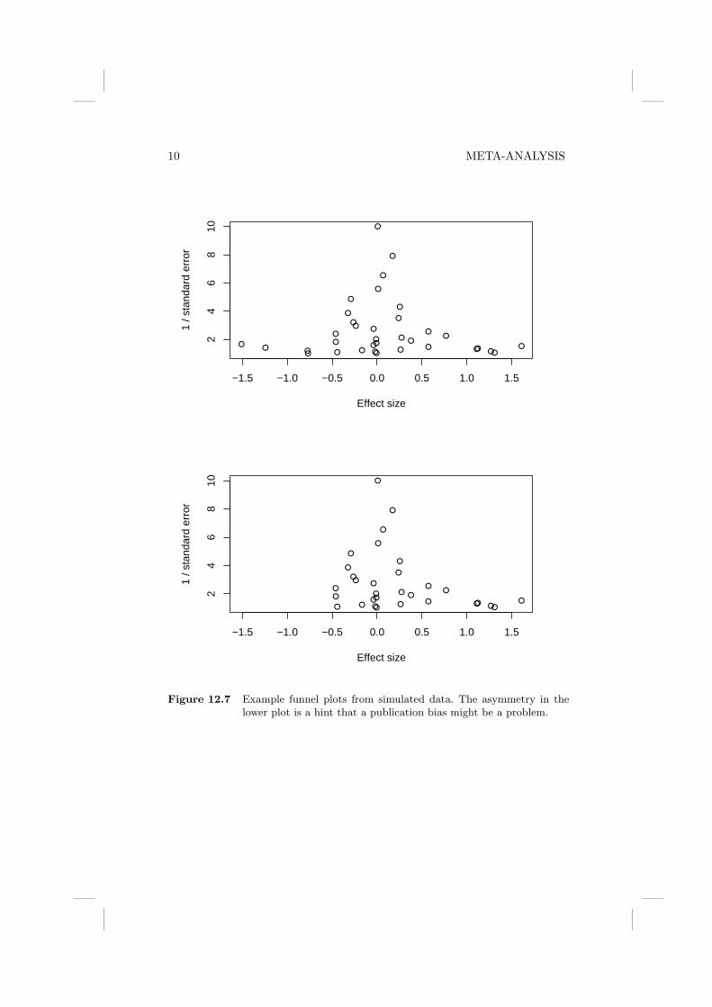
10 META-ANALYSIS
●
●
●
●
●●
●●
●● ● ●● ●●● ●● ●● ● ●●● ●●●●● ●●● ●●●
−1.5 −1.0 −0.5 0.0 0.5 1.0 1.5
24
68
10
Effect size
1 / s
tand
ard
erro
r
●
●
●
●
●●
●●
●● ● ●● ●●● ●● ●● ●● ●●●● ●●● ●●
−1.5 −1.0 −0.5 0.0 0.5 1.0 1.5
24
68
10
Effect size
1 / s
tand
ard
erro
r
Figure 12.7 Example funnel plots from simulated data. The asymmetry in thelower plot is a hint that a publication bias might be a problem.

PUBLICATION BIAS 11R> funnelplot(smokingDSL$logs, smokingDSL$selogs, summ = smokingDSL$logDSL,+ xlim = c(-1.7, 1.7))R> abline(v = 0, lty = 2)
●●
●
●
●
●
●●
●
●●
●●
●
●
●
●
●
●●
●
●
●
●
●
●
0.0 0.5 1.0 1.5
02
46
Effect
Siz
e
Figure 12.8 Funnel plot for nicotine gum data.

CHAPTER 13
Principal Component Analysis: TheOlympic Heptathlon
13.1 Introduction
13.2 Principal Component Analysis
13.3 Analysis Using R
To begin it will help to score all the seven events in the same direction, so that‘large’ values are ‘good’. We will recode the running events to achieve this;R> data("heptathlon", package = "HSAUR")R> heptathlon$hurdles <- max(heptathlon$hurdles) -+ heptathlon$hurdlesR> heptathlon$run200m <- max(heptathlon$run200m) -+ heptathlon$run200mR> heptathlon$run800m <- max(heptathlon$run800m) -+ heptathlon$run800m
Figure 13.1 shows a scatterplot matrix of the results from the 25 competitorson the seven events. We see that most pairs of events are positively correlatedto a greater or lesser degree. The exceptions all involve the javelin event –this is the only really ‘technical’ event and it is clear that training to becomesuccessful in the other six ‘power’-based events makes this event difficult forthe majority of the competitors. We can examine the numerical values of thecorrelations by applying the cor functionR> round(cor(heptathlon[, -score]), 2)
hurdles highjump shot run200m longjump javelin run800mhurdles 1.00 0.81 0.65 0.77 0.91 0.01 0.78highjump 0.81 1.00 0.44 0.49 0.78 0.00 0.59shot 0.65 0.44 1.00 0.68 0.74 0.27 0.42run200m 0.77 0.49 0.68 1.00 0.82 0.33 0.62longjump 0.91 0.78 0.74 0.82 1.00 0.07 0.70javelin 0.01 0.00 0.27 0.33 0.07 1.00 -0.02run800m 0.78 0.59 0.42 0.62 0.70 -0.02 1.00
This correlation matrix demonstrates again the points made earlier. A prin-cipal component analysis of the data can be applied using the prcomp func-tion. The result is a list containing the coefficients defining each component(sometimes referred to as loadings), the principal component scores, etc. Therequired code is (omitting the score variable)
3

4 PRINCIPAL COMPONENT ANALYSISR> score <- which(colnames(heptathlon) == "score")R> plot(heptathlon[, -score])
hurdles
1.50 1.75
●●●
●●●
●●●●
●●
●●● ●●
●●
●●●
●●
●
●●●
●●●
● ●●●●●
● ●● ●●
●●
●● ●
●●
●
0 2 4
●●●
●●●●●●●
●●
●●●●●
●●
●●●
●●
●
●●●
●●●●●●
●●●
●●● ●●
●●
●●●
●●
●
36 42
●●●
● ●●
●● ●●
●●
●●●●●
●●
●●●
●●
● 02
●●●
●●●
●●●●
●●
●● ●●●
●●
●●●
●●
●
1.50
1.75
●
●●
●
●
●●●
●
●
●
●
●●●
●
●●
●
●●
●●
●
●
highjump
●
●●
●
●
●● ●
●
●
●
●
●●
●
●
●●
●
●●
●●
●
●
●
●●
●
●
●●●
●
●
●
●
●●●
●
●●
●
●●
●●
●
●
●
●●
●
●
●●●
●
●
●
●
●●●
●
●●
●
●●
●●●
●
●
●●
●
●
●●●
●
●
●
●
●●
●
●
●●
●
● ●
●●●
●
●
●●
●
●
●●●
●
●
●
●
●●
●
●
●●
●
●●
●●
●
●
●●
●
●●
●●
●●
●● ●
●
●●
●
●●●●●
●
●●
●
●●
●
●●
●●
●●
●●●
●
●●
●
●●●●●
●
●●
●
shot
●●
●
●●
●●
●●
●● ●
●
●●
●
● ●●●●
●
●●
●
●●
●
●●
●●
●●
●●●
●
●●
●
●●●●●
●
●●
●
●●
●
●●
●●
● ●
●● ●
●
●●
●
● ●●● ●
●
●●
●
1013
16●●
●
●●
●●
●●
●●●
●
●●
●
●● ●●●
●
●●
●
02
4 ●
●●
●●
●
●
●●
●
●
●
●●●
●●
●●
●●●●
●●
●
●●
●●
●
●
●●
●
●
●
●●●●
●
●●
●●●●
●●
●
●●
●●
●
●
●●
●
●
●
● ●●●
●
●●
●● ●●
●●
run200m
●
●●
●●
●
●
●●
●
●
●
●●●
●●
●●
●●●●
●●
●
●●
● ●
●
●
●●
●
●
●
●●●●
●
●●
● ●●●
●●
●
●●
●●
●
●
●●
●
●
●
●● ●●
●
● ●
●●●●
●●
●
●●
●●●●●●
●● ●●●●● ●
●●●●●●●
●
●
●●
●● ●●●●
● ●●●●●●●
●● ●●
●●●
●
●
●●
●●●● ●●
●●●● ●●
●●●●●
●●● ●
●
●
● ●
●●● ●●●
●● ●●●●●●●●●
●●●●
●
longjump
●
● ●
● ●●●●●
●● ●●●●
●●●●●
●●●●
● 5.0
6.5
●
●●
●●●●●●●●●●● ●
● ●● ●●
●● ●●
●
3642
●
●
●●
●
●
●
●
●
●●
●
●
●●
●
●
●
●
●
●●●●
● ●
●
●●
●
●
●
●
●
●●
●
●
●●
●
●
●
●
●
●●●●
● ●
●
●●
●
●
●
●
●
●●
●
●
●●
●
●
●
●
●
● ●● ●
● ●
●
●●
●
●
●
●
●
●●
●
●
●●
●
●
●
●
●
●●●●
● ●
●
●●
●
●
●
●
●
●●
●
●
●●
●
●
●
●
●
●●●●
●
javelin
●
●
●●
●
●
●
●
●
●●
●
●
●●
●
●
●
●
●
●● ●●
●
0 2
●●●
●●●
●●●●● ●●
●●
●
●
●
●●●
●
●●
●
●●●
●● ●
●●●●●● ●
●●
●
●
●
●●●
●
●●
●
10 13 16
●●●
●●●
● ●●●●●●
●●
●
●
●
●●●
●
● ●
●
●● ●
●●●
●●● ●● ●●
●●
●
●
●
●●●
●
●●
●
5.0 6.5
●●●
●●●
●●●●●●●
●●
●
●
●
●●●
●
●●
●
●● ●
●●●
●● ●●● ● ●
●●
●
●
●
●● ●
●
●●
●
0 20 40
020
40run800m
Figure 13.1 Scatterplot matrix for the heptathlon data.
R> heptathlon_pca <- prcomp(heptathlon[, -score], scale = TRUE)R> print(heptathlon_pca)
Standard deviations:[1] 2.1119364 1.0928497 0.7218131 0.6761411 0.4952441 0.2701029[7] 0.2213617
Rotation:PC1 PC2 PC3 PC4
hurdles -0.4528710 0.15792058 -0.04514996 0.02653873highjump -0.3771992 0.24807386 -0.36777902 0.67999172shot -0.3630725 -0.28940743 0.67618919 0.12431725run200m -0.4078950 -0.26038545 0.08359211 -0.36106580longjump -0.4562318 0.05587394 0.13931653 0.11129249

ANALYSIS USING R 5
javelin -0.0754090 -0.84169212 -0.47156016 0.12079924run800m -0.3749594 0.22448984 -0.39585671 -0.60341130
PC5 PC6 PC7hurdles -0.09494792 -0.78334101 0.38024707highjump 0.01879888 0.09939981 -0.43393114shot 0.51165201 -0.05085983 -0.21762491run200m -0.64983404 0.02495639 -0.45338483longjump -0.18429810 0.59020972 0.61206388javelin 0.13510669 -0.02724076 0.17294667run800m 0.50432116 0.15555520 -0.09830963
The summary method can be used for further inspection of the details:R> summary(heptathlon_pca)
Importance of components:PC1 PC2 PC3 PC4 PC5 PC6
Standard deviation 2.112 1.093 0.7218 0.6761 0.4952 0.2701Proportion of Variance 0.637 0.171 0.0744 0.0653 0.0350 0.0104Cumulative Proportion 0.637 0.808 0.8822 0.9475 0.9826 0.9930
PC7Standard deviation 0.221Proportion of Variance 0.007Cumulative Proportion 1.000
The linear combination for the first principal component isR> a1 <- heptathlon_pca$rotation[, 1]R> a1
hurdles highjump shot run200m longjump-0.4528710 -0.3771992 -0.3630725 -0.4078950 -0.4562318
javelin run800m-0.0754090 -0.3749594
We see that the 200m and long jump competitions receive the highest weightbut the javelin result is less important. For computing the first principal com-ponent, the data need to be rescaled appropriately. The center and the scalingused by prcomp internally can be extracted from the heptathlon_pca viaR> center <- heptathlon_pca$centerR> scale <- heptathlon_pca$scale
Now, we can apply the scale function to the data and multiply with theloadings matrix in order to compute the first principal component score foreach competitorR> hm <- as.matrix(heptathlon[, -score])R> drop(scale(hm, center = center, scale = scale) %*%+ heptathlon_pca$rotation[, 1])
Joyner-Kersee (USA) John (GDR) Behmer (GDR)-4.121447626 -2.882185935 -2.649633766
Sablovskaite (URS) Choubenkova (URS) Schulz (GDR)-1.343351210 -1.359025696 -1.043847471

6 PRINCIPAL COMPONENT ANALYSIS
Fleming (AUS) Greiner (USA) Lajbnerova (CZE)-1.100385639 -0.923173639 -0.530250689Bouraga (URS) Wijnsma (HOL) Dimitrova (BUL)-0.759819024 -0.556268302 -1.186453832
Scheider (SWI) Braun (FRG) Ruotsalainen (FIN)0.015461226 0.003774223 0.090747709Yuping (CHN) Hagger (GB) Brown (USA)-0.137225440 0.171128651 0.519252646
Mulliner (GB) Hautenauve (BEL) Kytola (FIN)1.125481833 1.085697646 1.447055499
Geremias (BRA) Hui-Ing (TAI) Jeong-Mi (KOR)2.014029620 2.880298635 2.970118607Launa (PNG)6.270021972
or, more conveniently, by extracting the first from all precomputed principalcomponentsR> predict(heptathlon_pca)[, 1]
Joyner-Kersee (USA) John (GDR) Behmer (GDR)-4.121447626 -2.882185935 -2.649633766
Sablovskaite (URS) Choubenkova (URS) Schulz (GDR)-1.343351210 -1.359025696 -1.043847471Fleming (AUS) Greiner (USA) Lajbnerova (CZE)-1.100385639 -0.923173639 -0.530250689Bouraga (URS) Wijnsma (HOL) Dimitrova (BUL)-0.759819024 -0.556268302 -1.186453832
Scheider (SWI) Braun (FRG) Ruotsalainen (FIN)0.015461226 0.003774223 0.090747709Yuping (CHN) Hagger (GB) Brown (USA)-0.137225440 0.171128651 0.519252646Mulliner (GB) Hautenauve (BEL) Kytola (FIN)1.125481833 1.085697646 1.447055499
Geremias (BRA) Hui-Ing (TAI) Jeong-Mi (KOR)2.014029620 2.880298635 2.970118607Launa (PNG)6.270021972
The first two components account for 81% of the variance. A barplot of eachcomponent’s variance (see Figure 13.2) shows how the first two componentsdominate. A plot of the data in the space of the first two principal components,with the points labelled by the name of the corresponding competitor can beproduced as shown with Figure 13.3. In addition, the first two loadings for theevents are given in a second coordinate system, also illustrating the special roleof the javelin event. This graphical representation is known as biplot (?). Thecorrelation between the score given to each athlete by the standard scoringsystem used for the heptathlon and the first principal component score canbe found fromR> cor(heptathlon$score, heptathlon_pca$x[, 1])

ANALYSIS USING R 7R> plot(heptathlon_pca)
heptathlon_pca
Var
ianc
es
01
23
4
Figure 13.2 Barplot of the variances explained by the principal components.
[1] -0.9910978
This implies that the first principal component is in good agreement with thescore assigned to the athletes by official Olympic rules; a scatterplot of theofficial score and the first principal component is given in Figure 13.4.

8 PRINCIPAL COMPONENT ANALYSISR> biplot(heptathlon_pca, col = c("gray", "black"))
−0.4 −0.2 0.0 0.2 0.4 0.6
−0.
4−
0.2
0.0
0.2
PC1
PC
2
Jy−K
JohnBhmr Sblv
Chbn
SchlFlmn
Grnr
Ljbn
Borg
Wjns
Dmtr
SchdBranRtsl
Ypng
Hggr
Brwn
Mlln
Htnv
Kytl
Grms
H−In
Jn−M
Laun
−5 0 5
−6
−4
−2
02
4
hurdleshighjump
shotrun200m
longjump
javelin
run800m
Figure 13.3 Biplot of the (scaled) first two principal components.

ANALYSIS USING R 9R> plot(heptathlon$score, heptathlon_pca$x[, 1])
●
●●
●●●●
●
●●
●
●
●●●●
●
●
●●
●
●
●●
●
4500 5000 5500 6000 6500 7000
−4
−2
02
46
heptathlon$score
hept
athl
on_p
ca$x
[, 1]
Figure 13.4 Scatterplot of the score assigned to each athlete in 1988 and the firstprincipal component.

CHAPTER 14
Multidimensional Scaling: BritishWater Voles and Voting in US
Congress
14.1 Introduction
14.2 Multidimensional Scaling
14.3 Analysis Using R
We can apply classical scaling to the distance matrix for populations of watervoles using the R function cmdscale. The following code finds the classicalscaling solution and computes the two criteria for assessing the required num-ber of dimensions as described above.
R> data("watervoles", package = "HSAUR")R> voles_mds <- cmdscale(watervoles, k = 13, eig = TRUE)R> voles_mds$eig
[1] 7.359910e-01 2.626003e-01 1.492622e-01 6.990457e-02[5] 2.956972e-02 1.931184e-02 2.775558e-17 -1.139451e-02[9] -1.279569e-02 -2.849924e-02 -4.251502e-02 -5.255450e-02[13] -7.406143e-02
Note that some of the eigenvalues are negative. The criterion P2 can be com-puted by
R> sum(abs(voles_mds$eig[1:2]))/sum(abs(voles_mds$eig))
[1] 0.6708889
and the criterion suggested by Mardia et al. (1979) is
R> sum((voles_mds$eig[1:2])^2)/sum((voles_mds$eig)^2)
[1] 0.9391378
The two criteria for judging number of dimensions differ considerably, but bothvalues are reasonably large, suggesting that the original distances between thewater vole populations can be represented adequately in two dimensions. Thetwo-dimensional solution can be plotted by extracting the coordinates fromthe points element of the voles_mds object; the plot is shown in Figure 14.1.We shall now apply non-metric scaling to the voting behaviour shown in
Table ??. Non-metric scaling is available with function isoMDS from packageMASS (Venables and Ripley, 2002):
3
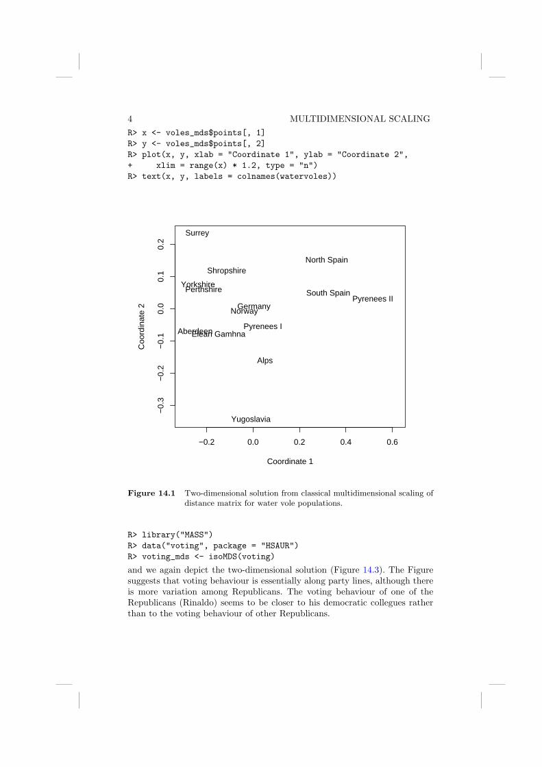
4 MULTIDIMENSIONAL SCALINGR> x <- voles_mds$points[, 1]R> y <- voles_mds$points[, 2]R> plot(x, y, xlab = "Coordinate 1", ylab = "Coordinate 2",+ xlim = range(x) * 1.2, type = "n")R> text(x, y, labels = colnames(watervoles))
−0.2 0.0 0.2 0.4 0.6
−0.
3−
0.2
−0.
10.
00.
10.
2
Coordinate 1
Coo
rdin
ate
2
Surrey
Shropshire
YorkshirePerthshire
AberdeenElean Gamhna
Alps
Yugoslavia
GermanyNorway
Pyrenees I
Pyrenees II
North Spain
South Spain
Figure 14.1 Two-dimensional solution from classical multidimensional scaling ofdistance matrix for water vole populations.
R> library("MASS")R> data("voting", package = "HSAUR")R> voting_mds <- isoMDS(voting)
and we again depict the two-dimensional solution (Figure 14.3). The Figuresuggests that voting behaviour is essentially along party lines, although thereis more variation among Republicans. The voting behaviour of one of theRepublicans (Rinaldo) seems to be closer to his democratic collegues ratherthan to the voting behaviour of other Republicans.

ANALYSIS USING R 5R> library("ape")R> st <- mst(watervoles)R> plot(x, y, xlab = "Coordinate 1", ylab = "Coordinate 2",+ xlim = range(x) * 1.2, type = "n")R> for (i in 1:nrow(watervoles)) {+ w1 <- which(st[i, ] == 1)+ segments(x[i], y[i], x[w1], y[w1])+ }R> text(x, y, labels = colnames(watervoles))
−0.2 0.0 0.2 0.4 0.6
−0.
3−
0.2
−0.
10.
00.
10.
2
Coordinate 1
Coo
rdin
ate
2
Surrey
Shropshire
YorkshirePerthshire
AberdeenElean Gamhna
Alps
Yugoslavia
GermanyNorway
Pyrenees I
Pyrenees II
North Spain
South Spain
Figure 14.2 Minimum spanning tree for the watervoles data.

6 MULTIDIMENSIONAL SCALINGR> x <- voting_mds$points[, 1]R> y <- voting_mds$points[, 2]R> plot(x, y, xlab = "Coordinate 1", ylab = "Coordinate 2",+ xlim = range(voting_mds$points[, 1]) * 1.2,+ type = "n")R> text(x, y, labels = colnames(voting))R> voting_sh <- Shepard(voting[lower.tri(voting)],+ voting_mds$points)
−5 0 5 10
−6
−4
−2
02
46
8
Coordinate 1
Coo
rdin
ate
2
Hunt(R)
Sandman(R)
Howard(D)
Thompson(D)
Freylinghuysen(R)
Forsythe(R)
Widnall(R)
Roe(D)Heltoski(D)
Rodino(D)Minish(D)
Rinaldo(R)
Maraziti(R)
Daniels(D)
Patten(D)
Figure 14.3 Two-dimensional solution from non-metric multidimensional scalingof distance matrix for voting matrix.

ANALYSIS USING R 7R> library("MASS")R> voting_sh <- Shepard(voting[lower.tri(voting)],+ voting_mds$points)R> plot(voting_sh, pch = ".", xlab = "Dissimilarity",+ ylab = "Distance", xlim = range(voting_sh$x),+ ylim = range(voting_sh$x))R> lines(voting_sh$x, voting_sh$yf, type = "S")
5 10 15
510
15
Dissimilarity
Dis
tanc
e
Figure 14.4 The Shepard diagram for the voting data shows some discrepanciesbetween the original dissimilarities and the multidimensional scalingsolution.


Bibliography
Mardia, K. V., Kent, J. T., and Bibby, J. M. (1979), Multivariate Analysis,London, UK: Academic Press.
Venables, W. N. and Ripley, B. D. (2002), Modern Applied Statistics withS , Springer, 4th edition, URL http://www.stats.ox.ac.uk/pub/MASS4/,ISBN 0-387-95457-0.

CHAPTER 15
Cluster Analysis: Classifying theExoplanets
15.1 Introduction
15.2 Cluster Analysis
15.3 Analysis Using R
Sadly Figure 15.2 gives no completely convincing verdict on the number ofgroups we should consider, but using a little imagination ‘little elbows’ canbe spotted at the three and five group solutions. We can find the number ofplanets in each group usingR> planet_kmeans3 <- kmeans(planet.dat, centers = 3)R> table(planet_kmeans3$cluster)
1 2 328 10 63
The centers of the clusters for the untransformed data can be computed usinga small convenience functionR> ccent <- function(cl) {+ f <- function(i) colMeans(planets[cl == i, ])+ x <- sapply(sort(unique(cl)), f)+ colnames(x) <- sort(unique(cl))+ return(x)+ }
which, applied to the three cluster solution obtained by k-means getsR> ccent(planet_kmeans3$cluster)
1 2 3mass 7.0532143 3.4360 1.6540635period 839.1644356 2420.5500 311.3897179eccen 0.5184643 0.2718 0.1777984
for the three cluster solution and, for the five cluster solution usingR> planet_kmeans5 <- kmeans(planet.dat, centers = 5)R> table(planet_kmeans5$cluster)
1 2 3 4 528 5 7 49 12
R> ccent(planet_kmeans5$cluster)
3

4 CLUSTER ANALYSISR> data("planets", package = "HSAUR")R> library("scatterplot3d")R> scatterplot3d(log(planets$mass), log(planets$period),+ log(planets$eccen), type = "h", angle = 55,+ scale.y = 0.7, pch = 16, y.ticklabs = seq(0,+ 10, by = 2), y.margin.add = 0.1)
−3 −2 −1 0 1 2 3
−5
−4
−3
−2
−1
0
0
2
4
6
8
10
log(planets$mass)
log(
plan
ets$
perio
d)
log(
plan
ets$
ecce
n)
●
●
●
●
●●
●
●
●●
●●
●
●
●
●
●
●●
●●
●
●
●
●
●
●
●
●
●
●●
●
●
● ●
●
●
●●
●●
●
●
●
●●
●
●●
● ●
●
●
●
●
●●
●●
●
●
●
●
●●
●
●●
●●
●
●●
●
●
●●
●
●
●
●
●
●
●
●
●
●
●
●
●
●
●
●
Figure 15.1 3D scatterplot of the logarithms of the three variables available foreach of the exoplanets.
1 2 3 4 5mass 2.2617857 14.3480 2.185714 1.6846122 8.595period 580.6828929 659.3976 2557.642857 282.2685965 1335.740eccen 0.4910714 0.3268 0.199000 0.1221082 0.473

ANALYSIS USING R 5R> rge <- apply(planets, 2, max) - apply(planets, 2,+ min)R> planet.dat <- sweep(planets, 2, rge, FUN = "/")R> n <- nrow(planet.dat)R> wss <- rep(0, 10)R> wss[1] <- (n - 1) * sum(apply(planet.dat, 2, var))R> for (i in 2:10) wss[i] <- sum(kmeans(planet.dat,+ centers = i)$withinss)R> plot(1:10, wss, type = "b", xlab = "Number of groups",+ ylab = "Within groups sum of squares")
●
●
●
●
●
●
●●
●●
2 4 6 8 10
24
68
1012
Number of groups
With
in g
roup
s su
m o
f squ
ares
Figure 15.2 Within-cluster sum of squares for different numbers of clusters forthe exoplanet data.
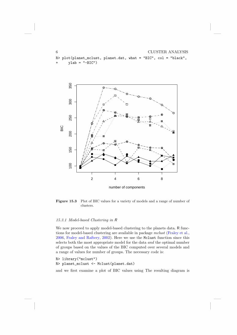
6 CLUSTER ANALYSISR> plot(planet_mclust, planet.dat, what = "BIC", col = "black",+ ylab = "-BIC")
2 4 6 8
100
150
200
250
300
350
number of components
BIC
●
● ●
●
●
●
●
●
●
●
●
●●
● ● ●●
●
●
●●
●
●
● ●
●
●
●
●●
●
●●
●
●
Figure 15.3 Plot of BIC values for a variety of models and a range of number ofclusters.
15.3.1 Model-based Clustering in R
We now proceed to apply model-based clustering to the planets data. R func-tions for model-based clustering are available in package mclust (Fraley et al.,2006, Fraley and Raftery, 2002). Here we use the Mclust function since thisselects both the most appropriate model for the data and the optimal numberof groups based on the values of the BIC computed over several models anda range of values for number of groups. The necessary code is:
R> library("mclust")R> planet_mclust <- Mclust(planet.dat)
and we first examine a plot of BIC values using The resulting diagram is

ANALYSIS USING R 7
shown in Figure 15.3. In this diagram the numbers refer to different modelassumptions about the shape of clusters:1. Spherical, equal volume,2. Spherical, unequal volume,3. Diagonal equal volume, equal shape,4. Diagonal varying volume, varying shape,5. Ellipsoidal, equal volume, shape and orientation,6. Ellipsoidal, varying volume, shape and orientation.The BIC selects model 4 (diagonal varying volume and varying shape) withthree clusters as the best solution as can be seen from the print output:R> print(planet_mclust)
best model: VVI with 3 components
This solution can be shown graphically as a scatterplot matrix The plot isshown in Figure 15.4. Figure 15.5 depicts the clustering solution in the three-dimensional space. The number of planets in each cluster and the meanvectors of the three clusters for the untransformed data can now be inspectedby usingR> table(planet_mclust$classification)
1 2 319 41 41
R> ccent(planet_mclust$classification)
1 2 3mass 1.16652632 1.5797561 6.0761463period 6.47180158 313.4127073 1325.5310048eccen 0.03652632 0.3061463 0.3704951
Cluster 1 consists of planets about the same size as Jupiter with very shortperiods and eccentricities (similar to the first cluster of the k-means solu-tion). Cluster 2 consists of slightly larger planets with moderate periods andlarge eccentricities, and cluster 3 contains the very large planets with verylarge periods. These two clusters do not match those found by the k-meansapproach.

8 CLUSTER ANALYSISR> x <- clPairs(planet.dat, classification = planet_mclust$classification,+ symbols = 1:3, col = "black")
mass
0.0 0.2 0.4 0.6 0.8 1.0
●●●●●●●●●●●●●●●●
●●●
0.0
0.2
0.4
0.6
0.8
1.0
●● ●● ●●● ●●●●●●● ●●
●●●
0.0
0.2
0.4
0.6
0.8
1.0
●●●●●●●●●●●●●●●● ●●●
period
●● ●● ●●● ●●●●●●● ●●●●●
0.0 0.2 0.4 0.6 0.8 1.0
●●
●
●
●
●●●●●●●●●
●●
●●● ●●
●
●
●
●●●●●●●●●
●●
●●●
0.0 0.2 0.4 0.6 0.8 1.0
0.0
0.2
0.4
0.6
0.8
1.0
eccen
Figure 15.4 Scatterplot matrix of planets data showing a three cluster solutionfrom Mclust.

ANALYSIS USING R 9R> scatterplot3d(log(planets$mass), log(planets$period),+ log(planets$eccen), type = "h", angle = 55,+ scale.y = 0.7, pch = planet_mclust$classification,+ y.ticklabs = seq(0, 10, by = 2), y.margin.add = 0.1)
−3 −2 −1 0 1 2 3
−5
−4
−3
−2
−1
0
0
2
4
6
8
10
log(planets$mass)
log(
plan
ets$
perio
d)
log(
plan
ets$
ecce
n)
●
●
●
●
●
●
●
●
●
●
●
●
●
Figure 15.5 3D scatterplot of planets data showing a three cluster solution fromMclust.


Bibliography
Fraley, C. and Raftery, A. E. (2002), “Model-based clustering, discriminantanalysis, and density estimation,” Journal of the American Statistical As-sociation, 97, 611–631.
Fraley, C., Raftery, A. E., and Wehrens, R. (2006), mclust: Model-based Clus-ter Analysis, URL http://www.stat.washington.edu/mclust, R packageversion 3.0-0.

CHAPTER 16
Errata
The document gives a list of typos, errors, inconsistencies etc. which have beenspotted. Moreover, small numeric output differences which are due to updatedpackages are reported here. To get a full list of differences run R CMD checkHSAUR on the source package.
Preface
Typo in name of vignette for Chapter 1, should readR> vignette("Ch_introduction_to_R", package = "HSAUR")
andR> edit(vignette("Ch_introduction_to_R", package = "HSAUR"))
As of version 1.0-3, only the correctly named vignette is available.
16.1 Introduction to R
Typo at page 20 (Ex. 1.5): number of companies, not number of countries.
16.2 Simple Inference
Typo at page 31, code line 4: use argument varwidth = TRUE, not var.width= TRUE.
16.3 Conditional Inference
• The names of the test statistics in the output have been changed from T toZ or chi-squared throughout the chapter.
• Reference Hothorn et al. (2006a) updated
16.4 Analysis of Variance
–nothing known–
16.5 Multiple Linear Regression
Page 83: both fitted and predict can be used to compute fitted values, thelater on can be applied to new unseen data as well.
3

4 ERRATA
16.6 Logistic Regression and Generalised Linear Models
Function myplot (page 100): the vfont argument in text has been changedto family = "HersheySerif" (the resulting plots remain the same).
16.7 Density Estimation
• Page 121: small numeric differences for the output of optim• update to mclust version 3.0-0 (new names of parameters in mclust objects)
16.8 Recursive Partitioning
• Page 139: small differences in predtab
• Page 140: small differences in table at bottom of this page• Reference Hothorn et al. (2006b) updated
16.9 Survival Analysis
The name of the test statistic in the output of surv_test has been changedto chi-squared.
16.10 Analysing Longitudinal Data I
Page 168, Figure 10.2: summary does not provide degrees of freedom and p-values in newer versions of lme4.
16.11 Analysing Longitudinal Data II
–nothing known–
16.12 Meta-Analysis
–nothing known–
16.13 Principal Component Analysis
–nothing known–
16.14 Multidimensional Scaling
–nothing known–
16.15 Cluster Analysis
update to mclust version 3.0-0 (new plot method)

CLUSTER ANALYSIS 5
Thanks
We would like to thank the following people for pointing out errors, typos etcand for making suggestions for improvements:• Tobias Verbeke• Brian D. Ripley


Bibliography
Hothorn, T., Hornik, K., van de Wiel, M. A., and Zeileis, A. (2006a),“A Lego system for conditional inference,” The American Statistician,60, 257–263, URL http://statmath.wu-wien.ac.at/~zeileis/papers/Hothorn+Hornik+VanDeWiel-2006.pdf.
Hothorn, T., Hornik, K., and Zeileis, A. (2006b), “Unbiased recursive parti-tioning: A conditional inference framework,” Journal of Computational andGraphical Statistics, 15, 651–674, URL http://statmath.wu-wien.ac.at/~zeileis/papers/Hothorn+Hornik+Zeileis-2006.pdf.

The HSAUR PackageNovember 2, 2006
Title A Handbook of Statistical Analyses Using R
Date $Date: 2006/10/21 16:18:55 $
Version 1.0-6
Author Brian S. Everitt and Torsten Hothorn
Maintainer Torsten Hothorn <[email protected]>
Description Functions, data sets, analyses and examples from the book ‘A Handbook of StatisticalAnalyses Using R’ (Brian S. Everitt and Torsten Hothorn, Chapman & Hall/CRC, 2006). Thefirst chapter of the book, which is entitled ‘An Introduction to R’, is completely included in thispackage, for all other chapters, a vignette containing all data analyses is available.
URL The publishers web page ishttp://www.crcpress.com/shopping_cart/products/product_detail.asp?sku=C5394
Depends R (>= 2.2.0), lattice, MASS, scatterplot3d (>= 0.3-23)
Suggests ape (>= 1.6), coin (>= 0.3-3), flexmix (>= 1.1-0), gee (>= 4.13-10), ipred (>= 0.8-3), lme4(>= 0.98-1), mclust (>= 3.0-0), party (>= 0.2-8), randomForest (>= 4.5-12), rmeta (>= 2.12), vcd(>= 0.9-3), survival
LazyData yes
License GPL
R topics documented:BCG . . . . . . . . . . . . . . . . . . . . . . . . . . . . . . . . . . . . . . . . . . . . . 2BtheB . . . . . . . . . . . . . . . . . . . . . . . . . . . . . . . . . . . . . . . . . . . . 3CYGOB1 . . . . . . . . . . . . . . . . . . . . . . . . . . . . . . . . . . . . . . . . . . 5Forbes2000 . . . . . . . . . . . . . . . . . . . . . . . . . . . . . . . . . . . . . . . . . 6HSAURtable . . . . . . . . . . . . . . . . . . . . . . . . . . . . . . . . . . . . . . . . 7Lanza . . . . . . . . . . . . . . . . . . . . . . . . . . . . . . . . . . . . . . . . . . . . 8aspirin . . . . . . . . . . . . . . . . . . . . . . . . . . . . . . . . . . . . . . . . . . . . 9birthdeathrates . . . . . . . . . . . . . . . . . . . . . . . . . . . . . . . . . . . . . . . . 10bladdercancer . . . . . . . . . . . . . . . . . . . . . . . . . . . . . . . . . . . . . . . . 10
1

2 BCG
clouds . . . . . . . . . . . . . . . . . . . . . . . . . . . . . . . . . . . . . . . . . . . . 11epilepsy . . . . . . . . . . . . . . . . . . . . . . . . . . . . . . . . . . . . . . . . . . . 12foster . . . . . . . . . . . . . . . . . . . . . . . . . . . . . . . . . . . . . . . . . . . . 13gardenflowers . . . . . . . . . . . . . . . . . . . . . . . . . . . . . . . . . . . . . . . . 14heptathlon . . . . . . . . . . . . . . . . . . . . . . . . . . . . . . . . . . . . . . . . . . 15mastectomy . . . . . . . . . . . . . . . . . . . . . . . . . . . . . . . . . . . . . . . . . 16meteo . . . . . . . . . . . . . . . . . . . . . . . . . . . . . . . . . . . . . . . . . . . . 17orallesions . . . . . . . . . . . . . . . . . . . . . . . . . . . . . . . . . . . . . . . . . . 18phosphate . . . . . . . . . . . . . . . . . . . . . . . . . . . . . . . . . . . . . . . . . . 18pistonrings . . . . . . . . . . . . . . . . . . . . . . . . . . . . . . . . . . . . . . . . . . 19planets . . . . . . . . . . . . . . . . . . . . . . . . . . . . . . . . . . . . . . . . . . . . 20plasma . . . . . . . . . . . . . . . . . . . . . . . . . . . . . . . . . . . . . . . . . . . . 21polyps . . . . . . . . . . . . . . . . . . . . . . . . . . . . . . . . . . . . . . . . . . . . 22pottery . . . . . . . . . . . . . . . . . . . . . . . . . . . . . . . . . . . . . . . . . . . . 23rearrests . . . . . . . . . . . . . . . . . . . . . . . . . . . . . . . . . . . . . . . . . . . 24respiratory . . . . . . . . . . . . . . . . . . . . . . . . . . . . . . . . . . . . . . . . . . 24roomwidth . . . . . . . . . . . . . . . . . . . . . . . . . . . . . . . . . . . . . . . . . . 25schizophrenia . . . . . . . . . . . . . . . . . . . . . . . . . . . . . . . . . . . . . . . . 26schizophrenia2 . . . . . . . . . . . . . . . . . . . . . . . . . . . . . . . . . . . . . . . 27schooldays . . . . . . . . . . . . . . . . . . . . . . . . . . . . . . . . . . . . . . . . . . 28skulls . . . . . . . . . . . . . . . . . . . . . . . . . . . . . . . . . . . . . . . . . . . . 29smoking . . . . . . . . . . . . . . . . . . . . . . . . . . . . . . . . . . . . . . . . . . . 30students . . . . . . . . . . . . . . . . . . . . . . . . . . . . . . . . . . . . . . . . . . . 31suicides . . . . . . . . . . . . . . . . . . . . . . . . . . . . . . . . . . . . . . . . . . . 32toothpaste . . . . . . . . . . . . . . . . . . . . . . . . . . . . . . . . . . . . . . . . . . 32voting . . . . . . . . . . . . . . . . . . . . . . . . . . . . . . . . . . . . . . . . . . . . 33water . . . . . . . . . . . . . . . . . . . . . . . . . . . . . . . . . . . . . . . . . . . . 34watervoles . . . . . . . . . . . . . . . . . . . . . . . . . . . . . . . . . . . . . . . . . . 35waves . . . . . . . . . . . . . . . . . . . . . . . . . . . . . . . . . . . . . . . . . . . . 36weightgain . . . . . . . . . . . . . . . . . . . . . . . . . . . . . . . . . . . . . . . . . . 37womensrole . . . . . . . . . . . . . . . . . . . . . . . . . . . . . . . . . . . . . . . . . 38
Index 39
BCG BCG Vaccine Data
Description
A meta-analysis on the efficacy of BCG vaccination against tuberculosis (TB).
Usage
data("BCG")
BtheB 3
Format
A data frame with 13 observations on the following 7 variables.
Study an identifier of the study.
BCGTB the number of subjects suffering from TB after a BCG vaccination.
BCGVacc the number of subjects with BCG vaccination.
NoVaccTB the number of subjects suffering from TB without BCG vaccination.
NoVacc the total number of subjects without BCG vaccination.
Latitude geographic position of the place the study was undertaken.
Year the year the study was undertaken.
Details
Bacille Calmette Guerin (BCG) is the most widely used vaccination in the world. Developed in the1930s and made of a live, weakened strain of Mycobacterium bovis, the BCG is the only vaccinationavailable against tuberculosis today. Colditz et al. (1994) report data from 13 clinical trials of BCGvaccine each investigating its efficacy in the treatment of tuberculosis. The number of subjectssuffering from TB with or without BCG vaccination are given here. In addition, the data containsthe values of two other variables for each study, namely, the geographic latitude of the place wherethe study was undertaken and the year of publication. These two variables will be used to investigateand perhaps explain any heterogeneity among the studies.
Source
G. A. Colditz, T. F. Brewer, C. S. Berkey, M. E. Wilson, E. Burdick, H. V. Fineberg and F. Mosteller(1994), Efficacy of BCG vaccine in the prevention of tuberculosis. Meta-analysis of the publishedliterature. Journal of the American Medical Association, 271(2), 698–702.
Examples
data("BCG", package = "HSAUR")boxplot(BCG$BCGTB/BCG$BCGVacc, BCG$NoVaccTB/BCG$NoVacc,
names = c("BCG Vaccination", "No Vaccination"),ylab = "Percent BCG cases")
BtheB Beat the Blues Data
Description
Data from a clinical trial of an interactive multimedia program called ‘Beat the Blues’.
Usage
data("BtheB")

4 BtheB
Format
A data frame with 100 observations of 100 patients on the following 8 variables.
drug did the patient take anti-depressant drugs (No or Yes).
length the length of the current episode of depression, a factor with levels <6m (less than sixmonths) and >6m (more than six months).
treatment treatment group, a factor with levels TAU (treatment as usual) and BtheB (Beat theBlues)
bdi.pre Beck Depression Inventory II before treatment.
bdi.2m Beck Depression Inventory II after two months.
bdi.4m Beck Depression Inventory II after four months.
bdi.6m Beck Depression Inventory II after six months.
bdi.8m Beck Depression Inventory II after eight months.
Details
Longitudinal data from a clinical trial of an interactive, multimedia program known as "Beat theBlues" designed to deliver cognitive behavioural therapy to depressed patients via a computer ter-minal. Patients with depression recruited in primary care were randomised to either the Beating theBlues program, or to "Treatment as Usual (TAU)".
Note that the data are stored in the wide form, i.e., repeated measurments are represented by addi-tional columns in the data frame.
Source
J. Proudfoot, D. Goldberg and A. Mann (2003). Computerised, interactive, multimedia CBT re-duced anxiety and depression in general practice: A RCT. Psychological Medicine, 33, 217–227.
Examples
data("BtheB", package = "HSAUR")layout(matrix(1:2, nrow = 1))ylim <- range(BtheB[,grep("bdi", names(BtheB))], na.rm = TRUE)boxplot(subset(BtheB, treatment == "TAU")[,grep("bdi", names(BtheB))],
main = "Treated as usual", ylab = "BDI",xlab = "Time (in months)", names = c(0, 2, 4, 6, 8), ylim = ylim)
boxplot(subset(BtheB, treatment == "BtheB")[,grep("bdi", names(BtheB))],main = "Beat the Blues", ylab = "BDI", xlab = "Time (in months)",names = c(0, 2, 4, 6, 8), ylim = ylim)

CYGOB1 5
CYGOB1 CYG OB1 Star Cluster Data
Description
Energy output and surface termperature for Star Cluster CYG OB1.
Usage
data("CYGOB1")
Format
A data frame with 47 observations on the following 2 variables.
logst log survface termperature of the star.
logli log light intensity of the star.
Details
The Hertzsprung-Russell (H-R) diagram forms the basis of the theory of stellar evolution. Thediagram is essentially a plot of the energy output of stars plotted against their surface temperature.Data from the H-R diagram of Star Cluster CYG OB1, calibrated according to VanismaGreve1972are given here.
Source
F. Vanisma and J. P. De Greve (1972), Close binary systems before and after mass transfer. Astro-physics and Space Science, 87, 377–401.
D. J. Hand, F. Daly, A. D. Lunn, K. J. McConway and E. Ostrowski (1994). A Handbook of SmallDatasets, Chapman and Hall/CRC, London.
Examples
data("CYGOB1", package = "HSAUR")plot(logst ~ logli, data = CYGOB1)

6 Forbes2000
Forbes2000 The Forbes 2000 Ranking of the World’s Biggest Companies (Year2004)
Description
The Forbes 2000 list is a ranking of the world’s biggest companies, measured by sales, profits,assets and market value.
Usage
data("Forbes2000")
Format
A data frame with 2000 observations on the following 8 variables.
rank the ranking of the company.
name the name of the company.
country a factor giving the country the company is situated in.
category a factor describing the products the company produces.
sales the amount of sales of the company in billion USD.
profits the profit of the company in billion USD.
assets the assets of the company in billion USD.
marketvalue the market value of the company in billion USD.
Source
http://www.forbes.com, assessed on November 26th, 2004.
Examples
data("Forbes2000", package = "HSAUR")summary(Forbes2000)### number of countrieslength(levels(Forbes2000$country))### number of industrieslength(levels(Forbes2000$category))

HSAURtable 7
HSAURtable Produce LaTeX Tables
Description
Generate longtable LaTeX environments.
Usage
HSAURtable(object, ...)## S3 method for class 'table':HSAURtable(object, xname = deparse(substitute(object)), pkg = NULL,
...)## S3 method for class 'data.frame':HSAURtable(object, xname = deparse(substitute(object)), pkg = NULL,
nrows = NULL, ...)## S3 method for class 'tabtab':toLatex(object, caption = NULL, label = NULL,
topcaption = TRUE, index = TRUE, ...)## S3 method for class 'dftab':toLatex(object, pcol = 1, caption = NULL,
label = NULL, rownames = FALSE, topcaption = TRUE, index = TRUE,...)
Arguments
object an object of table or data.frame.
xname the name of the object.
pkg the package object comes from, optionally.
nrows the number of rows actually printed for a data.frame.
caption the (optional) caption of the table without label.
label the (optional) label to be defined for this table.
pcol the number of parallel columns.
rownames logical, should the rownames be printed in the first row without column name?
topcaption logical, should the captions be placed on top (default) of the table?
index logical, should an index entry be generated?
... additional arguments, currently ignored.
Details
Based on the data in object, an object from which a Latex table (in a longtable environment)may be constructed (via toLatex) is generated.

8 Lanza
Value
An object of class tabtab or dftab for which toLatex methods are available.
toLatex produces objects of class Latex, a character vector, essentially.
Examples
data("rearrests", package = "HSAUR")toLatex(HSAURtable(rearrests),
caption = "Rearrests of juvenile felons.",label = "rearrests_tab")
Lanza Prevention of Gastointestinal Damages
Description
Data from four randomised clinical trials on the prevention of gastointestinal damages by Miso-prostol reported by Lanza et al. (1987, 1988a,b, 1989).
Usage
data("Lanza")
Format
A data frame with 198 observations on the following 3 variables.
study a factor with levels I, II, III, and IV describing the study number.
treatment a factor with levels Misoprostol Placebo
classification an ordered factor with levels 1 < 2 < 3 < 4 < 5 describing an ordered responsevariable.
Details
The response variable is defined by the number of haemorrhages or erosions.
Source
F. L. Lanza (1987), A double-blind study of prophylactic effect of misoprostol on lesions of gastricand duodenal mucosa induced by oral administration of tolmetin in healthy subjects. British Journalof Clinical Practice, May suppl, 91–101.
F. L. Lanza, R. L. Aspinall, E. A. Swabb, R. E. Davis, M. F. Rack, A. Rubin (1988a), Double-blind,placebo-controlled endoscopic comparison of the mucosal protective effects of misoprostol versuscimetidine on tolmetin-induced mucosal injury to the stomach and duodenum. Gastroenterology,95(2), 289–294.

aspirin 9
F. L. Lanza, K. Peace, L. Gustitus, M. F. Rack, B. Dickson (1988b), A blinded endoscopic compar-ative study of misoprostol versus sucralfate and placebo in the prevention of aspirin-induced gastricand duodenal ulceration. American Journal of Gastroenterology, 83(2), 143–146.
F. L. Lanza, D. Fakouhi, A. Rubin, R. E. Davis, M. F. Rack, C. Nissen, S. Geis (1989), A double-blind placebo-controlled comparison of the efficacy and safety of 50, 100, and 200 micrograms ofmisoprostol QID in the prevention of ibuprofen-induced gastric and duodenal mucosal lesions andsymptoms. American Journal of Gastroenterology, 84(6), 633–636.
Examples
data("Lanza", package = "HSAUR")layout(matrix(1:4, nrow = 2))pl <- tapply(1:nrow(Lanza), Lanza$study, function(indx)
mosaicplot(table(Lanza[indx,"treatment"],Lanza[indx,"classification"]),
main = "", shade = TRUE))
aspirin Aspirin Data
Description
Efficacy of Aspirin in preventing death after a myocardial infarct.
Usage
data("aspirin")
Format
A data frame with 7 observations on the following 4 variables.
dp number of deaths after placebo.
tp total number subjects treated with placebo.
da number of deaths after Aspirin.
ta total number of subjects treated with Aspirin.
Details
The data were collected for a meta-analysis of the effectiveness of Aspirin (versus placebo) inpreventing death after a myocardial infarction.
Source
J. L. Fleiss (1993), The statistical basis of meta-analysis. Statistical Methods in Medical Research2, 121–145.
10 bladdercancer
Examples
data("aspirin", package = "HSAUR")aspirin
birthdeathrates Birth and Death Rates Data
Description
Birth and death rates for 69 countries.
Usage
data("birthdeathrates")
Format
A data frame with 69 observations on the following 2 variables.
birth birth rate.
death death rate.
Source
J. A. Hartigan (1975), Clustering Algorithms. John Wiley & Sons, New York.
Examples
data("birthdeathrates", package = "HSAUR")plot(birthdeathrates)
bladdercancer Bladder Cancer Data
Description
Data arise from 31 male patients who have been treated for superficial bladder cancer, and give thenumber of recurrent tumours during a particular time after the removal of the primary tumour, alongwith the size of the original tumour.
Usage
data("bladdercancer")

clouds 11
Format
A data frame with 31 observations on the following 3 variables.
time the duration.
tumorsize a factor with levels <=3cm and >3cm.
number number of recurrent tumours.
Details
The aim is the estimate the effect of size of tumour on the number of recurrent tumours.
Source
G. U. H. Seeber (1998), Poisson Regression. In: Encyclopedia of Biostatistics (P. Armitage and T.Colton, eds), John Wiley & Sons, Chichester.
Examples
data("bladdercancer", package = "HSAUR")mosaicplot(xtabs(~ number + tumorsize, data = bladdercancer))
clouds Cloud Seeding Data
Description
Data from an experiment investigating the use of massive amounts of silver iodide (100 to 1000grams per cloud) in cloud seeding to increase rainfall.
Usage
data("clouds")
Format
A data frame with 24 observations on the following 7 variables.
seeding a factor indicating whether seeding action occured (no or yes).
time number of days after the first day of the experiment.
cloudcover the percentage cloud cover in the experimental area, measured using radar.
sne suitability criterion.
prewetness the total rainfall in the target area one hour before seeding (in cubic metres times1e+8).
echomotion a factor showing whether the radar echo was moving or stationary.
rainfall the amount of rain in cubic metres times 1e+8.

12 epilepsy
Details
Weather modification, or cloud seeding, is the treatment of individual clouds or storm systems withvarious inorganic and organic materials in the hope of achieving an increase in rainfall. Introductionof such material into a cloud that contains supercooled water, that is, liquid water colder than zeroCelsius, has the aim of inducing freezing, with the consequent ice particles growing at the expenseof liquid droplets and becoming heavy enough to fall as rain from clouds that otherwise wouldproduce none.
The data available in cloud were collected in the summer of 1975 from an experiment to inves-tigate the use of massive amounts of silver iodide 100 to 1000 grams per cloud) in cloud seedingto increase rainfall. In the experiment, which was conducted in an area of Florida, 24 days werejudged suitable for seeding on the basis that a measured suitability criterion (SNE).
Source
W. L. Woodley, J. Simpson, R. Biondini and J. Berkeley (1977), Rainfall results 1970-75: Floridaarea cumulus experiment. Science 195, 735–742.
Examples
data("clouds", package = "HSAUR")layout(matrix(1:2, nrow = 2))boxplot(rainfall ~ seeding, data = clouds, ylab = "Rainfall")boxplot(rainfall ~ echomotion, data = clouds, ylab = "Rainfall")
epilepsy Epilepsy Data
Description
A randomised clinical trial investigating the effect of an anti-epileptic drug.
Usage
data("epilepsy")
Format
A data frame with 236 observations on the following 6 variables.
treatment the treatment group, a factor with levels placebo and Progabide.
base the number of seizures before the trial.
age the age of the patient.
seizure.rate the number of seizures (response variable).
period treatment period, an ordered factor with levels 1 to 4.
subject the patient ID, a factor with levels 1 to 59.

foster 13
Details
In this clinical trial, 59 patients suffering from epilepsy were randomized to groups receiving eitherthe anti-epileptic drug Progabide or a placebo in addition to standard chemotherapy. The numbersof seizures suffered in each of four, two-week periods were recorded for each patient along with abaseline seizure count for the 8 weeks prior to being randomized to treatment and age. The mainquestion of interest is whether taking progabide reduced the number of epileptic seizures comparedwith placebo.
Source
P. F. Thall and S. C. Vail (1990), Some covariance models for longitudinal count data with overdis-persion. Biometrics, 46, 657–671.
Examples
data("epilepsy", package = "HSAUR")library(lattice)dotplot(I(seizure.rate / base) ~ period | subject, data = epilepsy,
subset = treatment == "Progabide")dotplot(I(seizure.rate / base) ~ period | subject, data = epilepsy,
subset = treatment == "Progabide")
foster Foster Feeding Experiment
Description
The data are from a foster feeding experiment with rat mothers and litters of four different geno-types. The measurement is the litter weight after a trial feeding period.
Usage
data("foster")
Format
A data frame with 61 observations on the following 3 variables.
litgen genotype of the litter, a factor with levels A, B, I, and J.
motgen genotype of the mother, a factor with levels A, B, I, and J.
weight the weight of the litter after a feeding period.
Details
Here the interest lies in uncovering the effect of genotype of mother and litter on litter weight.

14 gardenflowers
Source
D. J. Hand, F. Daly, A. D. Lunn, K. J. McConway and E. Ostrowski (1994). A Handbook of SmallDatasets, Chapman and Hall/CRC, London.
Examples
data("foster", package = "HSAUR")plot.design(foster)
gardenflowers Garden Flowers
Description
The dissimilarity matrix of 18 species of garden flowers.
Usage
data("gardenflowers")
Format
An object of class dist.
Details
The dissimilarity was computed based on certain characteristics of the flowers.
Source
L. Kaufman and P. J. Rousseeuw (1990), Finding groups in data: an introduction to cluster analysis,John Wiley & Sons, New York.
Examples
data("gardenflowers", package = "HSAUR")gardenflowers

heptathlon 15
heptathlon Olympic Heptathlon Seoul 1988
Description
Results of the olympic heptathlon competition, Seoul, 1988.
Usage
data("heptathlon")
Format
A data frame with 25 observations on the following 8 variables.
hurdles results 100m hurdles.
highjump results high jump.
shot results shot.
run200m results 200m race.
longjump results long jump.
javelin results javelin.
run800m results 800m race.
score total score.
Details
The first combined Olympic event for women was the pentathlon, first held in Germany in 1928.Initially this consisted of the shot putt, long jump, 100m, high jump and javelin events held overtwo days. The pentathlon was first introduced into the Olympic Games in 1964, when it consistedof the 80m hurdles, shot, high jump, long jump and 200m. In 1977 the 200m was replaced by the800m and from 1981 the IAAF brought in the seven-event heptathlon in place of the pentathlon,with day one containing the events-100m hurdles, shot, high jump, 200m and day two, the longjump, javelin and 800m. A scoring system is used to assign points to the results from each eventand the winner is the woman who accumulates the most points over the two days. The event madeits first Olympic appearance in 1984.
In the 1988 Olympics held in Seoul, the heptathlon was won by one of the stars of women’s athleticsin the USA, Jackie Joyner-Kersee. The results for all 25 competitors are given here.
Source
D. J. Hand, F. Daly, A. D. Lunn, K. J. McConway and E. Ostrowski (1994). A Handbook of SmallDatasets, Chapman and Hall/CRC, London.

16 mastectomy
Examples
data("heptathlon", package = "HSAUR")plot(heptathlon)
mastectomy Survival Times after Mastectomy of Breast Cancer Patients
Description
Survival times in months after mastectomy of women with breast cancer. The cancers are classifiedas having metastized or not based on a histochemical marker.
Usage
data("matectomy")
Format
A data frame with 42 observations on the following 3 variables.
time survival times in months.
event a logical indicating if the event was observed (TRUE) or if the survival time was censored(FALSE).
metastized a factor at levels yes and no.
Source
B. S. Everitt and S. Rabe-Hesketh (2001), Analysing Medical Data using S-PLUS, Springer, NewYork, USA.
Examples
data("mastectomy", package = "HSAUR")table(mastectomy$metastized)

meteo 17
meteo Meteorological Measurements for 11 Years
Description
Several meteorological measurements for a period between 1920 and 1931.
Usage
data("meteo")
Format
A data frame with 11 observations on the following 6 variables.
year the years.
rainNovDec rainfall in November and December (mm).
temp average July temperature.
rainJuly rainfall in July (mm).
radiation radiation in July (millilitres of alcohol).
yield average harvest yield (quintals per hectare).
Details
Carry out a principal components analysis of both the covariance matrix and the correlation ma-trix of the data and compare the results. Which set of components leads to the most meaningfulinterpretation?
Source
B. S. Everitt and G. Dunn (2001), Applied Multivariate Data Analysis, 2nd edition, Arnold, London.
Examples
data("meteo", package = "HSAUR")meteo

18 phosphate
orallesions Oral Lesions in Rural India
Description
The distribution of the oral lesion site found in house-to-house surveys in three geographic regionsof rural India.
Usage
data("orallesions")
Format
A two-way classification, see table.
Source
Cyrus R. Mehta and Nitin R. Patel (2003), StatXact-6: Statistical Software for Exact NonparametricInference, Cytel Software Cooperation, Cambridge, USA.
Examples
data("orallesions", package = "HSAUR")mosaicplot(orallesions)
phosphate Phosphate Level Data
Description
Plasma inorganic phosphate levels from 33 subjects.
Usage
data("phosphate")

pistonrings 19
Format
A data frame with 33 observations on the following 9 variables.
group a factor with levels control and obese.
t0 baseline phosphate level,
t0.5 phosphate level after 1/2 an hour.
t1 phosphate level after one an hour.
t1.5 phosphate level after 1 1/2 hours.
t2 phosphate level after two hours.
t3 phosphate level after three hours.
t4 phosphate level after four hours.
t5 phosphate level after five hours.
Source
C. S. Davis (2002), Statistical Methods for the Analysis of Repeated Measurements, Springer, NewYork.
Examples
data("phosphate", package = "HSAUR")plot(t0 ~ group, data = phosphate)
pistonrings Piston Rings Failures
Description
Number of failures of piston rings in three legs of four steam-driven compressors.
Usage
data("pistonrings")
Format
A two-way classification, see table.
Details
The data are given in form of a table. The table gives the number of piston-ring failures in eachof three legs of four steam-driven compressors located in the same building. The compressors haveidentical design and are oriented in the same way. The question of interest is whether the twoclassification variables (compressor and leg) are independent.

20 planets
Source
S. J. Haberman (1973), The analysis of residuals in cross-classificed tables. Biometrics 29, 205–220.
Examples
data("pistonrings", package = "HSAUR")mosaicplot(pistonrings)
planets Exoplanets Data
Description
Data on planets outside the Solar System.
Usage
data("planets")
Format
A data frame with 101 observations from 101 exoplanets on the following 3 variables.
mass Jupiter mass of the planet.
period period in earth days.
eccen the radial eccentricity of the planet.
Details
From the properties of the exoplanets found up to now it appears that the theory of planetary de-velopment constructed for the planets of the Solar System may need to be reformulated. The exo-planets are not at all like the nine local planets that we know so well. A first step in the process ofunderstanding the exoplanets might be to try to classify them with respect to their known properties.
Source
M. Mayor and P. Frei (2003). New Worlds in the Cosmos: The Discovery of Exoplanets. CambridgeUniversity Press, Cambridge, UK.

plasma 21
Examples
data("planets", package = "HSAUR")require("scatterplot3d")scatterplot3d(log(planets$mass), log(planets$period), log(planets$eccen),
type = "h", highlight.3d = TRUE, angle = 55,scale.y = 0.7, pch = 16)
plasma Blood Screening Data
Description
The erythrocyte sedimentation rate and measurements of two plasma proteins (fibrinogen and glob-ulin).
Usage
data("plasma")
Format
A data frame with 32 observations on the following 3 variables.
fibrinogen the fibrinogen level in the blood.
globulin the globulin level in the blood.
ESR the erythrocyte sedimentation rate, either less or greater 20 mm / hour.
Details
The erythrocyte sedimentation rate (ESR) is the rate at which red blood cells (erythrocytes) settleout of suspension in blood plasma, when measured under standard conditions. If the ESR increaseswhen the level of certain proteins in the blood plasma rise in association with conditions such asrheumatic diseases, chronic infections and malignant diseases, its determination might be useful inscreening blood samples taken form people suspected to being suffering from one of the conditionsmentioned. The absolute value of the ESR is not of great importance rather it is whether it is lessthan 20mm/hr since lower values indicate a healthy individual.
The question of interest is whether there is any association between the probability of an ESRreading greater than 20mm/hr and the levels of the two plasma proteins. If there is not then thedetermination of ESR would not be useful for diagnostic purposes.
Source
D. Collett and A. A. Jemain (1985), Residuals, outliers and influential observations in regressionanalysis. Sains Malaysiana, 4, 493–511.

22 polyps
Examples
data("plasma", package = "HSAUR")layout(matrix(1:2, ncol = 2))boxplot(fibrinogen ~ ESR, data = plasma, varwidth = TRUE)boxplot(globulin ~ ESR, data = plasma, varwidth = TRUE)
polyps Familial Andenomatous Polyposis
Description
Data from a placebo-controlled trial of a non-steroidal anti-inflammatory drug in the treatment offamilial andenomatous polyposis (FAP).
Usage
data("polyps")
Format
A data frame with 20 observations on the following 3 variables.
number number of colonic polyps at 12 months.
treat treatment arms of the trail, a factor with levels placebo and drug.
age the age of the patient.
Details
Giardiello et al. (1993) and Piantadosi (1997) describe the results of a placebo-controlled trial ofa non-steroidal anti-inflammatory drug in the treatment of familial andenomatous polyposis (FAP).The trial was halted after a planned interim analysis had suggested compelling evidence in favourof the treatment. Here we are interested in assessing whether the number of colonic polyps at 12months is related to treatment and age of patient.
Source
F. M. Giardiello, S. R. Hamilton, A. J. Krush, S. Piantadosi, L. M. Hylind, P. Celano, S. V. Booker,C. R. Robinson and G. J. A. Offerhaus (1993), Treatment of colonic and rectal adenomas withsulindac in familial adenomatous polyposis. New England Journal of Medicine, 328(18), 1313–1316.
S. Piantadosi (1997), Clinical Trials: A Methodologic Perspective. John Wiley & Sons, New York.

pottery 23
Examples
data("polyps", package = "HSAUR")plot(number ~ age, data = polyps, pch = as.numeric(polyps$treat))legend(40, 40, legend = levels(polyps$treat), pch = 1:2, bty = "n")
pottery Romano-British Pottery Data
Description
Chemical composition of Romano-British pottery.
Usage
data("pottery")
Format
A data frame with 45 observations on the following 9 chemicals.
Al2O3 aluminium trioxide.Fe2O3 iron trioxide.MgO magnesium oxide.CaO calcium oxide.Na2O natrium oxide.K2O calium oxide.TiO2 titanium oxide.MnO mangan oxide.BaO barium oxide.
Details
The data gives the chemical composition of specimens of Romano-British pottery, determined byatomic absorption spectrophotometry, for nine oxides.
Source
A. Tubb and N. J. Parker and G. Nickless (1980), The analysis of Romano-British pottery by atomicabsorption spectrophotometry. Archaeometry, 22, 153–171.
Examples
data("pottery", package = "HSAUR")plot(pottery)

24 respiratory
rearrests Rearrests of Juvenile Felons
Description
Rearrests of juventile felons by type of court in which they were tried.
Usage
data("rearrests")
Format
A two-way classification, see table.
Details
The data (taken from Agresti, 1996) arise from a sample of juveniles convicted of felony in Floridain 1987. Matched pairs were formed using criteria such as age and the number of previous offences.For each pair, one subject was handled in the juvenile court and the other was transferred to theadult court. Whether or not the juvenile was rearrested by the end of 1988 was then noted. Herethe question of interest is whether the true proportions rearrested were identical for the adult andjuvenile court assignments?
Source
A. Agresti (1996). An Introduction to Categorical Data Analysis. Wiley, New York.
Examples
data("rearrests", package = "HSAUR")rearrests
respiratory Respiratory Illness Data
Description
The respiratory status of patients recruited for a randomised clinical multicenter trial.
Usage
data("respiratory")

roomwidth 25
Format
A data frame with 555 observations on the following 7 variables.
centre the study center, a factor with levels 1 and 2.
treatment the treatment arm, a factor with levels placebo and treatment.
sex a factor with levels female and male.
age the age of the patient.
status the respiratory status (response variable), a factor with levels poor and good.
month the month, each patient was examined at months 0, 1, 2, 3 and 4.
subject the patient ID, a factor with levels 1 to 111.
Details
In each of two centres, eligible patients were randomly assigned to active treatment or placebo.During the treatment, the respiratory status (categorised poor or good) was determined at each offour, monthly visits. The trial recruited 111 participants (54 in the active group, 57 in the placebogroup) and there were no missing data for either the responses or the covariates. The question ofinterest is to assess whether the treatment is effective and to estimate its effect.
Note that the data are in long form, i.e, repeated measurments are stored as additional rows in thedata frame.
Source
C. S. Davis (1991), Semi-parametric and non-parametric methods for the analysis of repeated mea-surements with applications to clinical trials. Statistics in Medicine, 10, 1959–1980.
Examples
data("respiratory", package = "HSAUR")mosaicplot(xtabs( ~ treatment + month + status, data = respiratory))
roomwidth Students Estimates of Lecture Room Width
Description
Lecture room width estimated by students in two different units.
Usage
data("roomwidth")

26 schizophrenia
Format
A data frame with 113 observations on the following 2 variables.
unit a factor with levels feet and metres.
width the estimated width of the lecture room.
Details
Shortly after metric units of length were officially introduced in Australia, each of a group of 44students was asked to guess, to the nearest metre, the width of the lecture hall in which they weresitting. Another group of 69 students in the same room was asked to guess the width in feet, to thenearest foot. The data were collected by Professor T. Lewis and are taken from Hand et al (1994).The main question is whether estimation in feet and in metres gives different results.
Source
D. J. Hand, F. Daly, A. D. Lunn, K. J. McConway and E. Ostrowski (1994). A Handbook of SmallDatasets, Chapman and Hall/CRC, London.
Examples
data("roomwidth", package = "HSAUR")convert <- ifelse(roomwidth$unit == "feet", 1, 3.28)boxplot(I(width * convert) ~ unit, data = roomwidth)
schizophrenia Age of Onset of Schizophrenia Data
Description
Data on sex differences in the age of onset of schizophrenia.
Usage
data("schizophrenia")
Format
A data frame with 251 observations on the following 2 variables.
age age at the time of diagnosis.
gender a factor with levels female and male
schizophrenia2 27
Details
A sex difference in the age of onset of schizophrenia was noted by Kraepelin (1919). Subsequentlyepidemiological studies of the disorder have consistently shown an earlier onset in men than inwomen. One model that has been suggested to explain this observed difference is know as thesubtype model which postulates two type of schizophrenia, one characterised by early onset, typicalsymptoms and poor premorbid competence, and the other by late onset, atypical symptoms, andgood premorbid competence. The early onset type is assumed to be largely a disorder of men andthe late onset largely a disorder of women.
Source
E. Kraepelin (1919), Dementia Praecox and Paraphrenia. Livingstone, Edinburgh.
Examples
data("schizophrenia", package = "HSAUR")boxplot(age ~ gender, data = schizophrenia)
schizophrenia2 Schizophrenia Data
Description
Though disorder and early onset of schizophrenia.
Usage
data("schizophrenia2")
Format
A data frame with 220 observations on the following 4 variables.
subject the patient ID, a factor with levels 1 to 44.
onset the time of onset of the disease, a factor with levels < 20 yrs and > 20 yrs.
disorder whether thought disorder was absent or present, the response variable.
month month after hospitalisation.
Details
The data were collected in a follow-up study of women patients with schizophrenia. The binaryresponse recorded at 0, 2, 6, 8 and 10 months after hospitalisation was thought disorder (absent orpresent). The single covariate is the factor indicating whether a patient had suffered early or lateonset of her condition (age of onset less than 20 years or age of onset 20 years or above). Thequestion of interest is whether the course of the illness differs between patients with early and lateonset?

28 schooldays
Source
Davis (2002), Statistical Methods for the Analysis of Repeated Measurements, Springer, New York.
Examples
data("schizophrenia2", package = "HSAUR")mosaicplot(xtabs( ~ onset + month + disorder, data = schizophrenia2))
schooldays Days not Spent at School
Description
Data from a sociological study, the number of days absent from school is the response variable.
Usage
data("schooldays")
Format
A data frame with 154 observations on the following 5 variables.
race race of the child, a factor with levels aboriginal and non-aboriginal.
sex the sex of the child, a factor with levels female and male.
school the school type, a factor with levels F0 (primary), F1 (first), F2 (second) and F3 (thirdform).
learner how good is the child in learning things, a factor with levels average and slow.
absent number of days absent from school.
Details
The data arise from a sociological study of Australian Aboriginal and white children reported byQuine (1975).
In this study, children of both sexes from four age groups (final grade in primary schools and first,second and third form in secondary school) and from two cultural groups were used. The childrenin age group were classified as slow or average learners. The response variable was the number ofdays absent from school during the school year. (Children who had suffered a serious illness duringthe years were excluded.)
Source
S. Quine (1975), Achievement Orientation of Aboriginal and White Adolescents. Doctoral Disser-tation, Australian National University, Canberra.

skulls 29
Examples
data("schooldays", package = "HSAUR")plot.design(schooldays)
skulls Egyptian Skulls
Description
Measurements made on Egyptian skulls from five epochs.
Usage
data("skulls")
Format
A data frame with 150 observations on the following 5 variables.
epoch the epoch the skull as assigned to, a factor with levels c4000BC c3300BC, c1850BC,c200BC, and cAD150, where the years are only given approximately, of course.
mb maximum breaths of the skull.
bh basibregmatic heights of the skull.
bl basialiveolar length of the skull.
nh nasal heights of the skull.
Details
The question is whether the measurements change over time. Non-constant measurements of theskulls over time would indicate interbreeding with immigrant populations.
Source
D. J. Hand, F. Daly, A. D. Lunn, K. J. McConway and E. Ostrowski (1994). A Handbook of SmallDatasets, Chapman and Hall/CRC, London.
Examples
data("skulls", package = "HSAUR")means <- tapply(1:nrow(skulls), skulls$epoch, function(i)
apply(skulls[i,colnames(skulls)[-1]], 2, mean))means <- matrix(unlist(means), nrow = length(means), byrow = TRUE)colnames(means) <- colnames(skulls)[-1]rownames(means) <- levels(skulls$epoch)

30 smoking
pairs(means,panel = function(x, y) {
text(x, y, levels(skulls$epoch))})
smoking Nicotine Gum and Smoking Cessation
Description
Data from a meta-analysis on nicotine gum and smoking cessation
Usage
data("smoking")
Format
A data frame with 26 observations (studies) on the following 4 variables.
qt the number of treated subjetcs who stopped smoking.
tt the totla number of treated subjects.
qc the number of subjetcs who stopped smoking without being treated.
tc the total number of subject not being treated.
Details
Cigarette smoking is the leading cause of preventable death in the United States and kills moreAmericans than AIDS, alcohol, illegal drug use, car accidents, fires, murders and suicides com-bined. It has been estimated that 430,000 Americans die from smoking every year. Fighting to-bacco use is, consequently, one of the major public health goals of our time and there are now manyprograms available designed to help smokers quit. One of the major aids used in these programs isnicotine chewing gum, which acts as a substitute oral activity and provides a source of nicotine thatreduces the withdrawal symptoms experienced when smoking is stopped. But separate randomizedclinical trials of nicotine gum have been largely inconclusive, leading Silagy (2003) to considercombining the results studies found from an extensive literature search. The results of these trialsin terms of numbers of people in the treatment arm and the control arm who stopped smoking for atleast 6 months after treatment are given here.
Source
C. Silagy (2003), Nicotine replacement therapy for smoking cessation (Cochrane Review). TheCochrane Library, 4, John Wiley & Sons, Chichester.

students 31
Examples
data("smoking", package = "HSAUR")boxplot(smoking$qt/smoking$tt,
smoking$qc/smoking$tc,names = c("Treated", "Control"), ylab = "Percent Quitters")
students Student Risk Taking
Description
Students were administered two parallel forms of a test after a random assignment to three differenttreatments.
Usage
data("students")
Format
A data frame with 35 observations on the following 3 variables.
treatment a factor with levels AA, C, and NC.
low the result of the first test.
high the result of the second test.
Details
The data arise from a large study of risk taking (Timm, 2002). Students were randomly assigned tothree different treatments labelled AA, C and NC. Students were administered two parallel formsof a test called low and high. The aim is to carry out a test of the equality of the bivariate meansof each treatment population.
Source
N. H. Timm (2002), Applied Multivariate Analysis. Springer, New York.
Examples
data("students", package = "HSAUR")layout(matrix(1:2, ncol = 2))boxplot(low ~ treatment, data = students, ylab = "low")boxplot(high ~ treatment, data = students, ylab = "high")
32 toothpaste
suicides Crowd Baiting Behaviour and Suicides
Description
Data from a study carried out to investigate the causes of jeering or baiting behaviour by a crowdwhen a person is threatening to commit suicide by jumping from a high building.
Usage
data("suicides")
Format
A two-way classification, see table.
Source
L. Mann (1981), The baiting crowd in episodes of threatened suicide. Journal of Personality andSocial Psychology, 41, 703–709.
Examples
data("suicides", package = "HSAUR")mosaicplot(suicides)
toothpaste Toothpaste Data
Description
Meta-analysis of studies comparing two different toothpastes.
Usage
data("toothpaste")

voting 33
Format
A data frame with 9 observations on the following 7 variables.
Study the identifier of the study.
nA number of subjects using toothpaste A.
meanA mean DMFS index of subjects using toothpaste A.
sdA standard deviation of DMFS index of subjects using toothpaste A.
nB number of subjects using toothpaste B.
meanB mean DMFS index of subjects using toothpaste B.
sdB standard deviation of DMFS index of subjects using toothpaste B.
Details
The data are the results of nine randomised trials comparing two different toothpastes for the pre-vention of caries development. The outcomes in each trial was the change, from baseline, in thedecayed, missing (due to caries) and filled surface dental index (DMFS).
Source
B. S. Everitt and A. Pickles (2000), Statistical Aspects of the Design and Analysis of Clinical Trials,Imperial College Press, London.
Examples
data("toothpaste", package = "HSAUR")toothpaste
voting House of Representatives Voting Data
Description
Voting results for 15 congressmen from New Jersey.
Usage
data("voting")
Format
A 15 times 15 matrix.
34 water
Details
Romesburg (1984) gives a set of data that shows the number of times 15 congressmen from NewJersey voted differently in the House of Representatives on 19 environmental bills. Abstentions arenot recorded.
Source
H. C. Romesburg (1984), Cluster Analysis for Researchers. Lifetime Learning Publications, Bel-mont, Canada.
Examples
data("voting", package = "HSAUR")require("MASS")voting_mds <- isoMDS(voting)plot(voting_mds$points[,1], voting_mds$points[,2],
type = "n", xlab = "Coordinate 1", ylab = "Coordinate 2",xlim = range(voting_mds$points[,1])*1.2)
text(voting_mds$points[,1], voting_mds$points[,2],labels = colnames(voting))
voting_sh <- Shepard(voting[lower.tri(voting)], voting_mds$points)
water Mortality and Water Hardness
Description
The mortality and drinking water hardness for 61 cities in England and Wales.
Usage
data("water")
Format
A data frame with 61 observations on the following 4 variables.
location a factor with levels North and South indicating whether the town is as north as Derby.
town the name of the town.
mortality averaged annual mortality per 100.000 male inhabitants.
hardness calcium concentration (in parts per million).

watervoles 35
Details
The data were collected in an investigation of environmental causes of disease. They show theannual mortality per 100,000 for males, averaged over the years 1958-1964, and the calcium con-centration (in parts per million) in the drinking water for 61 large towns in England and Wales.The higher the calcium concentration, the harder the water. Towns at least as far north as Derbyare identified in the table. Here there are several questions that might be of interest including, aremortality and water hardness related, and do either or both variables differ between northern andsouthern towns?
Source
D. J. Hand, F. Daly, A. D. Lunn, K. J. McConway and E. Ostrowski (1994). A Handbook of SmallDatasets, Chapman and Hall/CRC, London.
Examples
data("water", package = "HSAUR")plot(mortality ~ hardness, data = water,
col = as.numeric(water$location))
watervoles Water Voles Data
Description
Percentage incidence of the 13 characteristics of water voles in 14 areas.
Usage
data("watervoles")
Format
A dissimilarity matrix for the following 14 variables, i.e, areas: Surrey, Shropshire,Yorkshire, Perthshire, Aberdeen, Elean Gamhna, Alps, Yugoslavia, Germany,Norway, Pyrenees I, Pyrenees II, North Spain, and South Spain.
Details
Corbet et al. (1970) report a study of water voles (genus Arvicola) in which the aim was to compareBritish populations of these animals with those in Europe, to investigate whether more than onespecies might be present in Britain. The original data consisted of observations of the presence orabsence of 13 characteristics in about 300 water vole skulls arising from six British populationsand eight populations from the rest of Europe. The data are the percentage incidence of the 13characteristics in each of the 14 samples of water vole skulls.

36 waves
Source
G. B. Corbet, J. Cummins, S. R. Hedges, W. J. Krzanowski (1970), The taxonomic structure ofBritish water voles, genus Arvicola. Journal of Zoology, 61, 301–316.
Examples
data("watervoles", package = "HSAUR")watervoles
waves Electricity from Wave Power at Sea
Description
Measurements of root mean square bending moment by two different mooring methods.
Usage
data("waves")
Format
A data frame with 18 observations on the following 2 variables.
method1 Root mean square bending moment in Newton metres, mooring method 1method2 Root mean square bending moment in Newton metres, mooring method 2
Details
In a design study for a device to generate electricity from wave power at sea, experiments werecarried out on scale models in a wave tank to establish how the choice of mooring method for thesystem affected the bending stress produced in part of the device. The wave tank could simulate awide range of sea states and the model system was subjected to the same sample of sea states witheach of two mooring methods, one of which was considerably cheaper than the other. The questionof interest is whether bending stress differs for the two mooring methods.
Source
D. J. Hand, F. Daly, A. D. Lunn, K. J. McConway and E. Ostrowski (1994). A Handbook of SmallDatasets, Chapman and Hall/CRC, London.
Examples
data("waves", package = "HSAUR")plot(method1 ~ method2, data = waves)

weightgain 37
weightgain Gain in Weight of Rats
Description
The data arise from an experiment to study the gain in weight of rats fed on four different diets,distinguished by amount of protein (low and high) and by source of protein (beef and cereal).
Usage
data("weightgain")
Format
A data frame with 40 observations on the following 3 variables.
source source of protein given, a factor with levels Beef and Cereal.
type amount of protein given, a factor with levels High and Low.
weightgain weigt gain in grams.
Details
Ten rats are randomized to each of the four treatments. The question of interest is how diet affectsweight gain.
Source
D. J. Hand, F. Daly, A. D. Lunn, K. J. McConway and E. Ostrowski (1994). A Handbook of SmallDatasets, Chapman and Hall/CRC, London.
Examples
data("weightgain", package = "HSAUR")interaction.plot(weightgain$type, weightgain$source,
weightgain$weightgain)

38 womensrole
womensrole Womens Role in Society
Description
Data from a survey from 1974 / 1975 asking both female and male responders about their opinionon the statement: Women should take care of running their homes and leave running the country upto men.
Usage
data("womensrole")
Format
A data frame with 42 observations on the following 4 variables.
education years of education.
sex a factor with levels Male and Female.
agree number of subjects in agreement with the statement.
disagree number of subjects in disagreement with the statement.
Details
The data are from Haberman (1973) and also given in Collett (2003). The questions here are whetherthe response of men and women differ.
Source
S. J. Haberman (1973), The analysis of residuals in cross-classificed tables. Biometrics, 29, 205–220.
D. Collett (2003), Modelling Binary Data. Chapman and Hall / CRC, London. 2nd edition.
Examples
data("womensrole", package = "HSAUR")summary(subset(womensrole, sex == "Female"))summary(subset(womensrole, sex == "Male"))

Index
∗Topic datasetsaspirin, 8BCG, 2birthdeathrates, 9bladdercancer, 9BtheB, 3clouds, 10CYGOB1, 4epilepsy, 11Forbes2000, 5foster, 12gardenflowers, 13heptathlon, 14Lanza, 7mastectomy, 15meteo, 16orallesions, 17phosphate, 17pistonrings, 18planets, 19plasma, 20polyps, 21pottery, 22rearrests, 23respiratory, 23roomwidth, 24schizophrenia, 25schizophrenia2, 26schooldays, 27skulls, 28smoking, 29students, 30suicides, 31toothpaste, 31voting, 32water, 33watervoles, 34waves, 35weightgain, 36
womensrole, 37∗Topic misc
HSAURtable, 6
aspirin, 8
BCG, 2birthdeathrates, 9bladdercancer, 9BtheB, 3
clouds, 10CYGOB1, 4
dist, 13
epilepsy, 11
Forbes2000, 5foster, 12
gardenflowers, 13
heptathlon, 14HSAURtable, 6
Lanza, 7
mastectomy, 15meteo, 16
orallesions, 17
phosphate, 17pistonrings, 18planets, 19plasma, 20polyps, 21pottery, 22
rearrests, 23respiratory, 23
39

40 INDEX
roomwidth, 24
schizophrenia, 25schizophrenia2, 26schooldays, 27skulls, 28smoking, 29students, 30suicides, 31
table, 17, 18, 23, 31toLatex, 6, 7toLatex.dftab (HSAURtable), 6toLatex.tabtab (HSAURtable), 6toothpaste, 31
voting, 32
water, 33watervoles, 34waves, 35weightgain, 36womensrole, 37