A Greedy Method for Solving Classes of PDE...

1

A Greedy Method for Solving Classes of PDE Problems

Robert Schaback1

Abstract: Motivated by the successful use of greedy algorithms for Reduced Ba-

sis Methods, a greedy method is proposed that selects N input data in an asymptot-

ically optimal way to solve well-posed operator equations using these N data. The

operator equations are defined as infinitely many equations given via a compact

set of functionals in the dual of an underlying Hilbert space, and then the greedy

algorithm, defined directly in the dual Hilbert space, selects N functionals step by

step. When N functionals are selected, the operator equation is numerically solved

by projection onto the span of the Riesz representers of the functionals. Orthonor-

malizing these yields useful Reduced Basis functions. By recent results on greedy

methods in Hilbert spaces, the convergence rate is asymptotically given by Kol-

mogoroff N-widths and therefore optimal in that sense. However, these N-widths

seem to be unknown in PDE applications. Numerical experiments show that for

solving elliptic second-order Dirichlet problems, the greedy method of this pa-

per behaves like the known P-greedy method for interpolation, applied to second

derivatives. Since the latter technique is known to realize Kolmogoroff N-widths

for interpolation, it is hypothesized that the Kolmogoroff N-widths for solving

second-order PDEs behave like the Kolmogoroff N-widths for second derivatives,

but this is an open theoretical problem.

Keywords: Operator equations, Greedy methods, Reduced Basis Methods, Kol-

mogoroff N-widths, Partial Differential Equations, meshless methods, colloca-

tion, discretization, error bounds, well-posedness, stability, convergence

Mathematics Subject Classification (2000): 65M12, 65M70, 65N12, 65N35,

65M15, 65J10, 41A25, 41A63

1Institut für Numerische und Angewandte Mathematik

Georg-August-Universität Göttingen, Lotzestraße 16–18, D-37083 Göttingen

[email protected], http://num.math.uni-goettingen.de/schaback/

1 INTRODUCTION 2

1 Introduction

For illustration of the application scope of this paper, consider the class of all

second-order elliptic boundary value problems

Lu = f on Ω ⊂ Rd

u = g on Γ := ∂Ω(1)

with arbitrary Dirichlet data and a fixed second-order strongly elliptic operator

L on a fixed bounded Lipschitz domain Ω ⊂ Rd . We keep this problem class in

strong form and pose it in Sobolev space W m2 (Rd) with m > 2+ d/2 and spaces

of data functions f and g of corresponding smoothness. Similar to Reduced Basis

(e.g. [14, 1, 3, 6]) or Proper Orthogonal Decomposition methods (e.g. [15, 13,

10]), we focus on a class of PDE problems, not on single problems. The output

of this paper will be connected to both areas, since a “reduced” orthonormal basis

is produced that is adapted to the given class of PDE problems.

The next section will generalize such problems to operator equations defined by

sets Λ of infinitely many functionals on an underlying Hilbert space of functions,

e.g. a Sobolev space. In this context, well-posedness can be formulated, and

for N selected functionals in a set ΛN ⊂ Λ, numerical solutions can be obtained

by Hilbert space projection on the Riesz representers of these functionals. This

is the well-known Rayleigh-Ritz idea. For kernel-based spaces, it coincides with

Symmetric Collocation and yields the optimal recovery technique in Hilbert space

for the given data functionals.

Section 3 analyzes the error in terms of the Generalized Power Function

PΛN(λ ) := dist(λ , span (ΛN))

on the dual of the Hilbert space and introduces

σΛN:= max

λ∈ΛPΛN

(λ )

that controls the error of the numerical solution in Hilbert space.

The greedy method of Section 4 now selects

λN+1 := arg maxPΛN(λ )

2 HILBERT SPACE THEORY 3

and follows the results of the literature on Reduced Basis Methods, linking the

decay of σΛNto Kolmogoroff N-widths.

For operator equations defined on Hilbert spaces of functions on a bounded do-

main Ω, the additional quantity

ρΛN:= max

x∈ΩPΛN

(δx)

directly controls the pointwise and uniform error in the domain, but is not useful

for greedy methods. For well-posed problems, Section 3.2 will show that ρΛN

is bounded form above by σΛNup to a factor, and numerical results in the final

Section 6 suggest that this bound is asymptotically sharp.

Before that, Section 5 gives a partial analysis of expectable Kolmogoroff N-widths

for second-order Dirichlet problems in Sobolev spaces W m2 . It is hypothesized

that both σΛNand the N-width behave like O(N−m−2−d/2

d ) for N → ∞, which is

the Kolmogoroff N-width for interpolation problems in W m−22 with respect to the

supremum norm. Section 6 shows supporting examples and concludes the paper.

2 Hilbert Space Theory

Following [11, 21] the problem class is written in terms of infinitely many con-

straints, each defined by a linear functional. The functional sets then are

Λ1 := δx L : x ∈ ΩΛ2 := δx : x ∈ Γ := ∂Ω

(2)

combined into Λ :=Λ1∪Λ2. Since all single functionals are continuous on W m2 (Rd),

the above sets are images of compact sets by continuous maps, thus compact. This

brings us into line with the literature on reduced basis methods.

The above problems are well-posed in the sense that there is a standard well-

posedness inequality of the form [2, 1.5, p. 30]

‖u‖∞,Ω ≤ ‖u‖∞,∂Ω +C‖Lu‖∞,Ω ≤ (C+1) supλ∈Λ

|λ (u)| for all u ∈C2(Ω)∪C(Γ).

(3)

3 ERROR ANALYSIS OF PROJECTION METHODS 4

2.1 Abstract Problem

Generalizing this case, and following [11, 21], we assume a Hilbert space H and

a subset Λ of its dual H ∗ that is total in the sense that

λ (u) = 0 for all λ ∈ Λ implies u = 0.

If we formally introduce the linear data map DΛ : H → RΛ with

DΛ(u) := λ (u)λ∈Λ for all u ∈ H ,

this means that elements u ∈ H are uniquely identifiable from their data DΛ(u).The central background problem in this paper is to recover elements u from their

data DΛ(u) in practice, i.e. the approximate numerical inversion of the data map.

In view of the preceding example we assume that the set Λ is compact.

The invertibility of the data map is quantified by assuming a well-posedness in-

equality

‖u‖WP ≤CW P‖DΛ(u)‖∞ =CWP supλ∈Λ

|λ (u)| for all u ∈ H (4)

in some well-posedness norm ‖.‖WP on H that usually is weaker than the norm

on H . Recall that [21] allows also to handle weakly formulated problems as

well this way. Furthermore, the framework applies to general operator equations,

including the case of interpolation if the operator is the identity.

3 Error Analysis of Projection Methods

For a finite subset ΛN := λ1, . . . ,λN of Λ we can define the subspace

LN := span ΛN ⊆ H∗

and use the Riesz representers vλ1, . . . ,vλN

of λ1, . . . ,λN as trial functions. They

span a space VΛNthat will lead later to reduced bases.

The standard optimal recovery of an element u∈H from finite data λ1(u), . . . ,λN(u)then proceeds by Hilbert space projection, i.e. by solving the linear system

λk(u) =N

∑j=1

α jλk(vλ j) =

N

∑j=1

α j(vλk,vλ j

)H =N

∑j=1

α j(λk,λ j)H ∗ , 1 ≤ k ≤ N


to get the numerical approximation

uN :=N

∑j=1

α jvλ j.

This satisfies the orthogonality relation

‖u‖2H = ‖u− uN‖

2H +‖uN‖

2H (5)

that implies uniform stability in Hilbert space. In case of the example in the be-

ginning, the method is known as Symmetric Collocation. This is a numerical

technique [7] based on [23] with certain optimality properties [20] and a conver-

gence theory [9, 8]. Within the Hilbert space framework, it produces pointwise

optimal approximations to the true solution under all possible methods that use

the same data [20].

3.1 Power Function

The standard error analysis in Hilbert Spaces uses the generalized Power Function

defined as

PΛN(µ) := min

λ∈LN

‖µ −λ‖H ∗ =: dist(µ,LN)H ∗ for all µ ∈ H∗. (6)

This is continuous and attains its maximum on the compact set Λ. In particular,

we are interested in

σΛN:= sup

λ∈Λ

PΛN(λ ) = sup

λ∈Λ

dist(λ ,LN)H ∗. (7)

3.2 Error Analysis

This quantity leads to error bounds for the discretized recovery problem that we

described in the beginning of this section.

Lemma 1. Let u ∈ H supply the finite data λ1(u), . . . ,λN(u) that is used to con-

struct uN by projection, and assume well-posedness in the sense of (4). Then

‖u− uN‖WP ≤ CWPσΛN‖u‖H .


Proof. Since u and uN share the same data, the assertion follows from

‖u− uN‖W P ≤ CW P supλ∈Λ |λ (u)−λ (uN)|= CW P supλ∈Λ |(λ −µ)(u− uN)| for all µ ∈ LN

(8)

using orthogonality (5) and well-posedness (4).

Therefore we are interested to find sets ΛN that minimize σΛNunder all sets of N

functionals from Λ.

By the same argument, for all continuous test functionals µ the inequality

|µ(u)−µ(uN)| ≤ PΛN(µ)‖u‖H , (9)

holds and we can check derivative errors once we evaluate the Generalized Power

Function on derivative functionals. Taking all functionals of Λ here, we get

‖DΛ(u− uN)‖∞ = supλ∈Λ

|λ (u− uN)| ≤ σΛN‖u‖H ,

i.e. σΛNbounds the error in the data norm.

In case of a Hilbert space H containing continuous functions on some compact

set Ω, there is a special case of (9) in the pointwise form

|u(x)− uN(x)| ≤ PΛN(δx)‖u‖H (10)

that may be checked by evaluation of the Generalized Power Function over all

delta functionals for all points of the domain. If we define

ρΛN:= max

x∈ΩPΛN

(δx) (11)

we get a uniform bound

‖u− uN‖∞,Ω ≤ ρΛN‖u‖H (12)

that is numerically available, and similar to the well-posedness inequality (3).

By definition, the Generalized Power Function decreases at all functionals when

we extend the set ΛN . All of these error bounds will then improve. For fixed ΛN

and H , they are optimal, but here we are interested in finding good finite subsets

ΛN of Λ.


Note that both Lemma 1 and (12) furnish similar error bounds with associated

convergence rates, and they might have the same behavior if the well-posedness

norm ‖.‖WP coincides with ‖.‖L∞(Ω). We shall have a closer look at this now,

delaying experiments to Section 6.

To find a connection between ρΛNand σΛN

in well-posed situations, we assume

that the well-posedness norm ‖.‖WP of (4) can be written as

‖u‖WP = supµ∈M

|µ(u)|, u ∈ H (13)

with a compact set M ⊂ H ∗, i.e. M is norming for ‖.‖WP. This yields (3) when

taking M as the set of delta functionals on Ω. The generalization of (11) then is

ρM,ΛN:= max

µ∈MPΛN

(µ). (14)

Lemma 2. Assuming (4) and (13), we have

ρM,ΛN≤CWPσΛN

.

Proof. The maximum in (14) is attained at some µN ∈ M and then

ρM,ΛN= PΛN

(µN)= dist(µN , span ΛN)

=

∥

∥

∥

∥

∥

µN −N

∑j=1

(µN ,µ j)µ j

∥

∥

∥

∥

∥

H ∗

.

Applied to an arbitrary u ∈ H this yields

∣

∣

∣µN(u)−∑N

j=1(µN ,µ j)µ j(u)∣

∣

∣= |µN(u)− µN(uN)|

≤ supµ∈M |µ(u)−µ(uN)|

= ‖u− uN‖W P

≤ CW P supλ∈Λ |λ (u)−λ (uN)|≤ CW PσΛN

‖u‖H

where the last line follows like (9) using a generalization of the argument within

(10).

4 GREEDY METHOD 8

4 Greedy Method

Given a set ΛN := λ1, . . . ,λN, the P-greedy algorithm [5, 18] in its abstract form

defines λN+1 recursively via

PΛN(λN+1) = sup

λ∈Λ

PΛN(λ ). (15)

In the context of Reduced Basis Methods in Hilbert spaces, this algorithm coin-

cides with the one in [14, 1, 3, 6]. The main difference is that we work in the dual

here, focusing on a single class of PDEs in applications instead of a parametrized

family. A first application of Reduced Basis Methods within a Reproducing Ker-

nel Hilbert Space setting is in [4], implementing a greedy method based on dis-

crete least-squares, not on the dual of the basic Hilbert space of functions.

The cited papers provide a useful error analysis of the method that we state here

for completeness. The main ingredient is the Kolmogorov N-width

dN(Λ) := infall HN

supµ∈Λ

infλ∈HN

‖λ −µ‖H ∗ = infall HN

supµ∈Λ

dist(µ,HN)H ∗

where the first infimum is taken over all N-dimensional subspaces HN ⊆ H ∗, not

only those spanned by N functionals from Λ. Then [6] proves

σ 22N(Λ)≤ 2dN(Λ),

while [1] has

σΛN≤C(α)N−α for n ∈ N, if dN(Λ)≤C′(α)N−α for n ∈ N

with suitable constants. This links the behaviour of the P-greedy algorithm to Kol-

mogoroff N-widths. The paper [18] exploits this connection for function recovery

by interpolation, while this paper extends [18] to classes of operator equations,

including PDE solving.

Consequently, the greedy method converges roughly like the Kolmogoroff N-

widths. Asymptotically, there are no better choices for selecting N functionals

out of Λ. Note that this works for all well-posed problems stated in abstract form

in Hilbert space via infinitely many constraints. The differential and boundary

operators can be easily generalized.

4 GREEDY METHOD 9

On the downside, the literature does not provide much information about the Kol-

mogoroff N-widths in such situations. This is why on has to look at special cases.

We postpone this to Section 5.

If we run the greedy algorithm numerically, we should get very good candidates

for reduced bases. Choosing them with additional orthogonality properties will

then bring us close to Proper Orthogonal Decomposition methods. The next sec-

tion will explain how to do that.

4.1 Implementation

Throughout, we assume that the Hilbert space H has a kernel K such that inner

products in H ∗ can be numerically calculated via

(λ ,µ)H ∗ = λ xµyK(x,y) for all λ , µ ∈ H∗

where the upper index stands for the variable the functional acts on. In case of

Sobolev spaces W m2 (Rd) with m> d/2, we use the standard Whittle-Matérn kernel

Km,d(x,y) = ‖x− y‖m−d/2

2 Km−d/2(‖x− y‖2), x,y ∈ Rd

with the modified Bessel function Kν of second kind. In what follows, we treat Λas being very large and finite, but extensions to infinite compact Λ will be possible

if functions on Λ are discretized somehow.

A direct way to assess the generalized Power Function at λ for given ΛN :=λ1, . . . ,λN is to use its definition via the approximation problem

infα∈RN

∥

∥

∥

∥

∥

λ −N

∑j=1

α jλ j

∥

∥

∥

∥

∥

2

H ∗

= P2ΛN

(λ ).

We assume that we have turned λ1, . . . ,λN into an H∗-orthonormal basis µ1, . . . ,µN

already, and then the solution is

P2ΛN

(λ ) =

∥

∥

∥

∥

∥

λ −N

∑j=1

(λ ,µ j)H ∗µ j

∥

∥

∥

∥

∥

2

H ∗

= (λ ,λ )H ∗ −N

∑j=1

(λ ,µ j)2H ∗. (16)

Furthermore, we store the orthonormalization system for getting the µ j from the

λ j as

µk =k−1

∑j=1

ck jµ j + ck,kλk, 1 ≤ k ≤ N. (17)

4 GREEDY METHOD 10

Besides the N ×N triangular matrix C, we store the values (λ ,λ )H ∗λ∈Λ and

(λ ,µk)H ∗λ∈Λ for k = 1, . . . ,N. These make up the method’s bulk storage of or-

der (N +1)|Λ|. Note that (λ ,λ )H ∗λ∈Λ simplifies considerably for translation-

invariant kernels.

After maximizing (16) over all λ ∈ Λ, we assume to have some λN+1 at which

a nonzero maximum is attained. This can then not be one of the old λ j, and we

retrieve the values (λN+1,µk)H ∗ from what we have. We now orthonormalize

µN+1 =N

∑j=1

cN+1, jµ j + cN+1,N+1λN+1

via cN+1, j =−(λN+1,µk)H ∗cN+1,N+1, 1 ≤ k ≤ N and

1 = (µN+1,µN+1)H ∗ = c2N+1,N+1

(

(λN+1,λN+1)H ∗ −N

∑k=1

(λN+1,µk)2H ∗

)

= c2N+1,N+1P2

ΛN(λN+1)

to update the C matrix. Finally

(λ ,µN+1)H ∗ =N

∑j=1

cN+1, j(λ ,µ j)H ∗ + cN+1,N+1(λ ,λN+1)H ∗

can be calculated from what we have, if we first calculate all (λ ,λN+1)H ∗λ∈Λ

and overwrite them with (λ ,µN+1)H ∗λ∈Λ after use. This extends the Newton

basis technique in [16] to general functionals.

4.2 Bases and Postprocessing

Useful reduced bases for PDE solving are the Riesz representers vµkof the µk,

being orthonormal in Hilbert space. From Riesz representers vλ j(·) = λ x

j K(x, ·) of

the λ j, we can calculate them recursively via

vµk(x) =

k−1

∑j=1

ck jvµ j(x)+ ck,k vλk

(x), 1 ≤ k ≤ n (18)

on whatever point sets we like, using our triangular matrix C. Via (16) in the form

P2ΛN

(δx) = K(x,x)−N

∑j=1

v2µ j(x), (19)

4 GREEDY METHOD 11

this allows to calculate the pointwise error bounds (10) described in Section 3.2

explicitly, up to the term ‖u‖H .

In view of Proper Orthogonal Decomposition, one can also apply a Singular Value

Decomposition to the partial Gramian matrix with entries (λ j,λk)H ∗, 1≤ j,k ≤N

and construct a different H -orthonormal basis. This possibility is not pursued

here, because we want to keep the recursive structure of the algorithm. In view of

[17], this basis may be closer to what happens for Kolmogoroff N-widths, because

the spaces for the latter will not necessarily have a recursive structure.

Like in reduced basis techniques, the orthonormal bases are a simple tool to solve

a variety of similar problems, namely all problems of the form (1). If data λ j(u)are known for an unknown function u, we go over to µ j(u) via the triangular

system (17) and then form the optimal projection

uN :=N

∑j=1

µ j(u)vµ j(20)

using the H -orthonormal basis we have constructed.

Note that this algorithm neither stores nor solves a large |Λ|×|Λ| system. It works

“on–the–fly”. For N steps, storage is of order O(N · |Λ|+N2) and calculations

are of order O(N2 · |Λ|). For a given accuracy requirement, the number N of steps

will depend on the Kolmogoroff N-width for the set Λ and the Hilbert space H ∗.

There are no square systems to be solved. Instead, there are N orthonormalization

steps on vectors of length |Λ| that may require standard stabilization precautions

for the basic Gram-Schmidt technique. The resulting triangular N ×N matrix C

is not explicitly inverted, but used via (17) to transform input data in terms of the

λ j functionals into data in terms of the orthonormalized functionals µ j. The error

behavior of this is comparable to backsubstitution after an LR or QR factorization,

but it will pay the price when some of the λ j are strongly correlated. This will be

unavoidable for large N, but (6) and (15) show that λN+1 will be kept away from

the zeros λ1, . . . ,λN of PΛNand the space they span, by construction.

4.3 Extended Greedy Method

One can get somewhat closer to the error analysis in Section 3.2 and in particu-

lar to (9) by a modification of the selection strategy of functionals. Given a set

5 SOBOLEV CASE 12

ΛN := λ1, . . . ,λN, and a set M = µ1, . . . ,µM with nonempty intersection, we

calculate two maxima

λ := argsupλ∈Λ PΛN(λ ) = σΛN

µ := argsupµ∈M PΛN(µ) =: ρΛN

and set

λN+1 :=

µ if µ ∈ Λ∩M

λ else.

This can be called an extended P-greedy algorithm. It tries to keep some additional

control of ρM,ΛNfrom (14) by selecting functionals from Λ∩M whenever ρM,ΛN

is attained on them.

For solving Dirichlet problems, the set M will consist of delta functionals in Ω,

the intersection of M and Λ being Λ2, the set of functionals for Dirichlet boundary

values. The new technique will make sure that if PΛN(M) attains its maximum on

the boundary, the corresponding functional is preferred over the functional where

PλN(Λ) attains its maximum.

Now for some inplementation details for the Dirichlet case. Define the set Z of

boundary points via

δz : z ∈ Z= Λ2

and add some other point set Y ⊂ Ω to get

M := δy : y ∈ Y∪Λ2 = δx : x ∈ Y ∪Z.

We need the additional value ‖PΛN‖∞,Y , while the usual Greedy method provides

‖PΛN‖∞,Z as part of the calculation of ρΛN

. If we use (19) on Y , we have the

necessary data, but for that we have to evaluate (18) on Y as well, and have to

store the values of the orthonormal basis on Y . This requires an additional storage

of size |Y | ·N for N steps, and additional calculations of order |Y | ·N2. On can

choose |Y | smaller than |Λ1| to keep the complexity at bay.

5 Sobolev case

We now go back to the example at the beginning. We need information on the

Kolmogoroff N-width

dN(Λ) = infall HN

supµ∈Λ

dist(µ,HN)W m2 (Ω)∗

5 SOBOLEV CASE 13

where the infimum is taken over all N-dimensional subspaces HN of H ∗=W m2 (Ω)∗,

and the set Λ = Λ1 ∪Λ2 ⊂ H ∗ is formed by (2). There should be an m- and d-

dependent decay rate κ(m,d) in the sense

dN(Λ)≤CN−κ(m,d) for N → ∞

but no explicit results on this were found yet.

If we restrict attention to spaces HN being generated by N functionals from Λ =Λ1 ∪Λ2 ⊂ H ∗, we only get an upper bound for dN(Λ), and we do not know

the splitting N = N1 +N2 if an optimal choice of N functionals from Λ takes N1

functionals out of Λ1 and N2 functionals out of Λ2. The rest of the chapter will

give some arguments supporting the hypothesis

κ(m,d)≥m−2−d/2

d(21)

that will be observed in the numerical behavior of the P-greedy method in Section

6.

If Λ is the union of two disjoint compact sets Λ1 and Λ2, then

dN(Λ) = infall HN

supµ∈Λ

dist(µ,HN)H ∗

= infall HN

max

(

supµ∈Λ1

dist(µ,HN)H ∗, supµ∈Λ2

dist(µ,HN)H ∗

)

≤ infHN1

,HN2,N1+N2≤N,HN=HN1

+HN2

max(dN1(Λ1),dN2

(Λ2))

where HNiis used for approximation of Λi, and the sum of spaces is direct. This

splitting argument is similar to the technique in [8]. However, we do not know a

priori how the greedy algorithm selects functionals from either set, and how the

dimension splits into N1 +N2 ≤ N.

We first aim at dN(Λ1) in the space W m2 (Ω)∗. We have

dN(Λ1) = infall HN

supx∈Ω

infλ∈HN

‖λ −δx L‖W m2 (Ω)∗

and can majorise it by choosing N asymptotically uniformly placed points x1, . . .xN

in Ω at fill distance hΩ and taking HN to be the span of the corresponding func-

tionals δx jL. Then

dN(Λ1) ≤ supx∈Ω

infα∈RN

‖δx L−N

∑j=1

α jδx jL‖W m

2 (Ω)∗

5 SOBOLEV CASE 14

holds and we can expect

dN(Λ1) ≤ C supx∈Ω

infα∈RN

‖δx −N

∑j=1

α jδx j‖

W m−22 (Ω)

∗

≤ C hm−2−d/2

Ω ≤C N−(m−2−d/2)/d

due to standard results on error bounds for interpolation [22], and with generic

constants depending on m, d and the domain.

On the boundary Γ, we can argue similarly to expect

dN(Λ2)≤C hm−d/2Γ ≤C N−m−d/2

d−1

for a fill distance hΓ on the boundary, either by working in W m2 (Ω)∗ directly, or

via trace theorems, which would give the same rate due to m−1/2− (d−1)/2 =m−d/2.

If we now consider splittings N = N1 +N2, we roughly have the upper bound

dN(Λ)≤C max

(

N−(m−2−d/2)/d

1 ,N−

m−d/2d−1

2

)

and the crude split N1 ≈ N/2 ≈ N2 will already support (21).

For purposes of asymptotics, we can minimize the sum of the above quantities

instead of the maximum. Using standard optimization arguments under the con-

straint N1 +N2 ≤ N, the result after some calculations is that one should expect

c1m−2−d/2

dN−

m−2+d/2d

1 = c2m−d/2

d−1N−

m−1+d/2d−1

2

with constants depending on the domain and the space dimension, but not on N

and m. For the typical case m = 4, d = 2 this implies N2 ≈ N3/8

1 . For large m

and d we get N1 ≈ N2, i.e. the domain and the boundary require roughly the same

degrees of freedom. This is no miracle, because the volumes of balls of high

dimension are increasingly accounted for by the boundary layer. In general, the

above argument implies N2 ≤ cN1 for N large enough, and then (21) will hold.

Section 6 will reveal that the greedy algorithm selects unexpectedly small values

of N2, and that the hypothesis (21) is supported.

6 NUMERICAL RESULTS 15

6 Numerical Results

No matter which PDE examples are selected, the most interesting question is the

behavior of the greedy method as a function of the N steps it takes. If Λ is chosen

large enough but still finite, the crucial quantities are σΛNand ρΛN

as defined in

(7) and (11). By Section 4 we can expect that σΛNdecays at an optimal rate

comparable to the Kolmogoroff N-width with respect to Λ, but since the latter

is still unknown, we can not yet assess how close we come to it. Since ρΛNis

controlling the error in the sup norm, without being usable for greedy refinement,

and in view of Lemma 2, we would like to confirm that ρΛNdecays as fast as

σΛN. And, the decay rates should improve with smoothness of the functions in

the basic Hilbert space, i.e. with m if we work in W m2 (Rd), our hypothesis being

(21). Another interesting question is how the greedy method chooses between

boundary functionals from Λ2 and domain functionals from Λ1, and whether the

corresponding points are roughly uniformly distributed in both cases. Finally,

the shape and the behaviour of the basis functions vµ jshould be demonstrated.

MATLAB code for all examples can be requested from the author.

6.1 Observations for varying N

We start on the 2D unit disk, with L being the Laplace operator, carrying the

greedy method out for up to 500 steps, offering 17570 functionals for Λ1 and 150

functionals for Λ2. The Hilbert space will be W m2 (R2), but we fix m > 2+ d/2

first, to study the behaviour of the greedy method for varying the number N of

steps. Classical results on kernel-based interpolation lets us expect rates for σΛN

and ρΛNthat are determined by fill distances. If hΓ and hΩ are fill distances for

points on the boundary Γ and in the domain Ω, we can compare σΛNwith plain

interpolation of ∆u = f with smoothness m−2 and behavior

hm−2−d/2

Ω = hm−3Ω ≈ N

−m−2−d/2

d

Ω = N−m−3

2

Ω (22)

on the domain. The error on the boundary in L∞ should, if it were a plain interpo-

lation, behave like

hm−1/2−(d−1)/2

Γ = hm−d/2

Γ = hm−1Γ ≈ N

−m−d/2d−1

Γ = N−(m−1)Γ , (23)

if NΓ points are asymptotically equally spaced on the boundary. But we do not

know a priori how the greedy algorithm chooses between boundary and domain

functionals.


The first experiments are for m = 4 > 2+ d/2 = 3, and we ignore the split N =NΩ +NΓ in the beginning. The scale of the Whittle-Matérn kernel is chosen to

be 1, and then both types of functionals happen to have the same norm. Scal-

ing changes the relation between function value evaluation and Laplace operator

evaluation and must be used with care. We wanted to eliminate scaling effects for

what follows, in order to let the choice between boundary and domain functionals

be unbiased by possibly different norms.

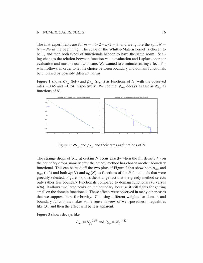
Figure 1 shows σΛN(left) and ρΛN

(right) as functions of N, with the observed

rates −0.45 and −0.54, respectively. We see that ρΛNdecays as fast as σΛN

as

functions of N.

0 1 2 3 4 5 6 7−2

−1.5

−1

−0.5

0

0.5

1

1.5

2Loglog plot of PF maximum, Rate = −0.54329, factor= 6.3439

0 1 2 3 4 5 6 7−2

−1.5

−1

−0.5

0

0.5

1

1.5Loglog plot of PF on deltas, Rate = −0.449676, factor= 2.84393

Figure 1: σΛNand ρΛN

and their rates as functions of N

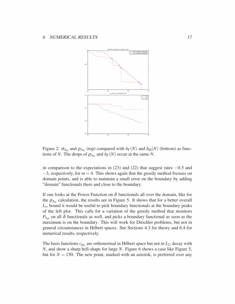
The strange drops of ρΛNat certain N occur exactly when the fill density hΓ on

the boundary drops, namely after the greedy method has chosen another boundary

functional. This can be read off the two plots of Figure 2 that show both σΛNand

ρΛN(left) and both hΓ(N) and hΩ(N) as functions of the N functionals that were

greedily selected. Figure 4 shows the strange fact that the greedy method selects

only rather few boundary functionals compared to domain functionals (6 versus

494). It allows two large peaks on the boundary, because it still fights for getting

small on the domain functionals. These effects were observed in many other cases

that we suppress here for brevity. Choosing different weights for domain and

boundary functionals makes some sense in view of well-posedness inequalities

like (3), and then the effect will be less apparent.

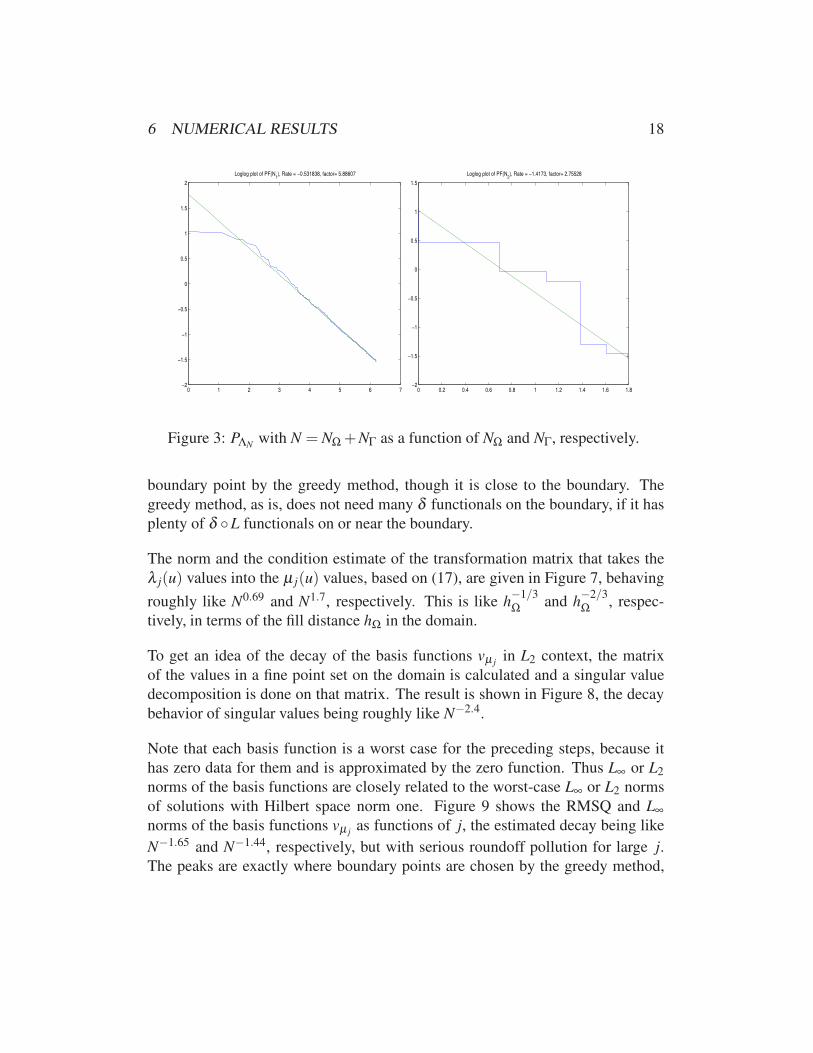
Figure 3 shows decays like

PΛN≈ N−0.53

Ω and PΛN≈ N−1.42

Γ


100

101

102

103

100

Both PF maxima as functions of N

PF on PDE functionalsPF on delta functionals

100

101

102

103

10−2

10−1

100

101

hB and h

D as functions of N

hB

hD


(top) compared with hΓ(N) and hΩ(N) (bottom) as func-

tions of N. The drops of ρΛNand hΓ(N) occur at the same N.

in comparison to the expectations in (23) and (22) that suggest rates −0.5 and

−3, respectively, for m = 4. This shows again that the greedy method focuses on

domain points, and is able to maintain a small error on the boundary by adding

“domain” functionals there and close to the boundary.

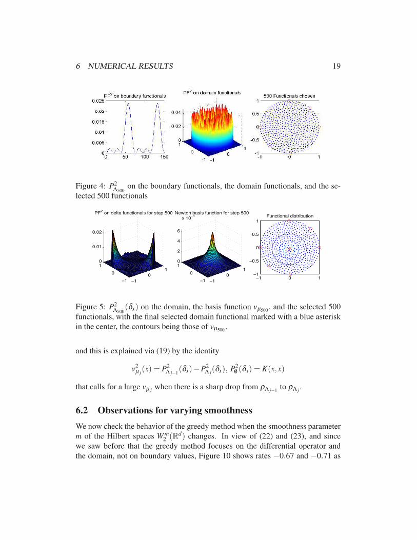
If one looks at the Power Function on δ functionals all over the domain, like for

the ρΛNcalculation, the results are in Figure 5. It shows that for a better overall

L∞ bound it would be useful to pick boundary functionals at the boundary peaks

of the left plot. This calls for a variation of the greedy method that monitors

PΛNon all δ functionals as well, and picks a boundary functional as soon as the

maximum is on the boundary. This will work for Dirichlet problems, but not in

general circumstances in Hilbert spaces. See Sections 4.3 for theory and 6.4 for

numerical results, respectively.

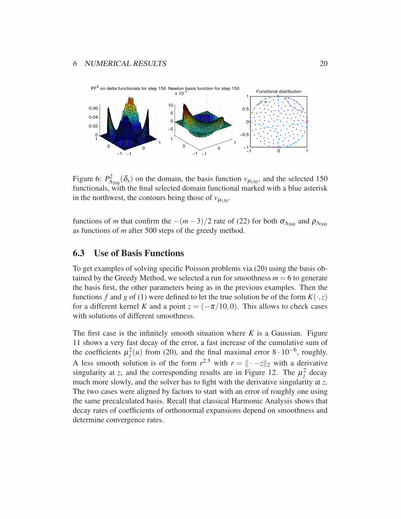
The basis functions vµNare orthonormal in Hilbert space but not in L2, decay with

N, and show a sharp bell-shape for large N. Figure 6 shows a case like Figure 5,

but for N = 150. The new point, marked with an asterisk, is preferred over any


0 1 2 3 4 5 6 7−2

−1.5

−1

−0.5

0

0.5

1

1.5

2

Loglog plot of PF(N1), Rate = −0.531838, factor= 5.88607

0 0.2 0.4 0.6 0.8 1 1.2 1.4 1.6 1.8−2

−1.5

−1

−0.5

0

0.5

1

1.5

Loglog plot of PF(N2), Rate = −1.4173, factor= 2.75528

Figure 3: PΛNwith N = NΩ +NΓ as a function of NΩ and NΓ, respectively.

boundary point by the greedy method, though it is close to the boundary. The

greedy method, as is, does not need many δ functionals on the boundary, if it has

plenty of δ L functionals on or near the boundary.

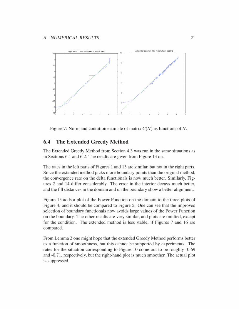
The norm and the condition estimate of the transformation matrix that takes the

λ j(u) values into the µ j(u) values, based on (17), are given in Figure 7, behaving

roughly like N0.69 and N1.7, respectively. This is like h−1/3

Ω and h−2/3

Ω , respec-

tively, in terms of the fill distance hΩ in the domain.

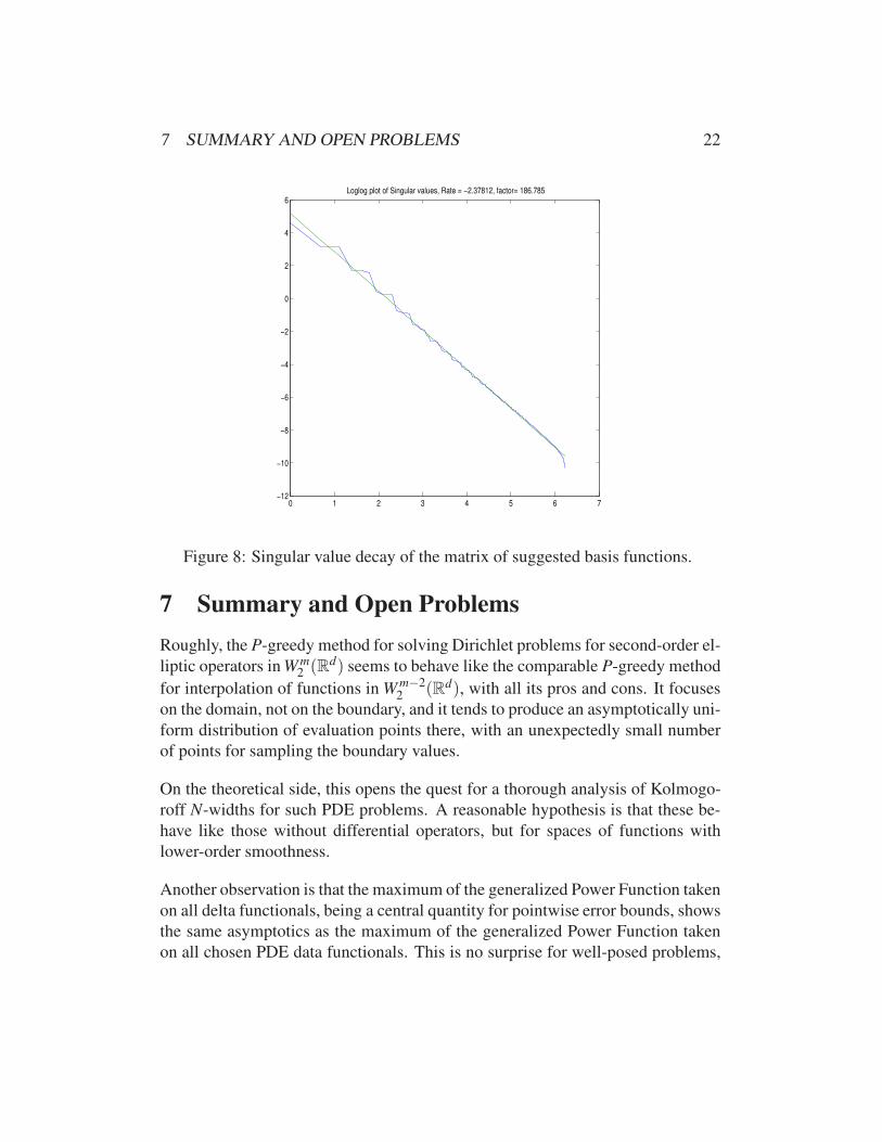
To get an idea of the decay of the basis functions vµ jin L2 context, the matrix

of the values in a fine point set on the domain is calculated and a singular value

decomposition is done on that matrix. The result is shown in Figure 8, the decay

behavior of singular values being roughly like N−2.4.

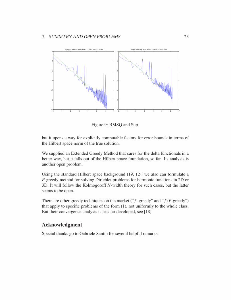
Note that each basis function is a worst case for the preceding steps, because it

has zero data for them and is approximated by the zero function. Thus L∞ or L2

norms of the basis functions are closely related to the worst-case L∞ or L2 norms

of solutions with Hilbert space norm one. Figure 9 shows the RMSQ and L∞

norms of the basis functions vµ jas functions of j, the estimated decay being like

N−1.65 and N−1.44, respectively, but with serious roundoff pollution for large j.

The peaks are exactly where boundary points are chosen by the greedy method,


Figure 4: P2Λ500

on the boundary functionals, the domain functionals, and the se-

lected 500 functionals

−1

0

1

−1

0

10

0.01

0.02

PF2 on delta functionals for step 500

−1

0

1

−1

0

10

2

4

6

x 10−4

Newton basis function for step 500

−1 0 1−1

−0.5

0

0.5

1Functional distribution

Figure 5: P2Λ500

(δx) on the domain, the basis function vµ500, and the selected 500

functionals, with the final selected domain functional marked with a blue asterisk

in the center, the contours being those of vµ500.

and this is explained via (19) by the identity

v2µ j(x) = P2

Λ j−1(δx)−P2

Λ j(δx), P2

/0 (δx) = K(x,x)

that calls for a large vµ jwhen there is a sharp drop from ρΛ j−1

to ρΛ j.

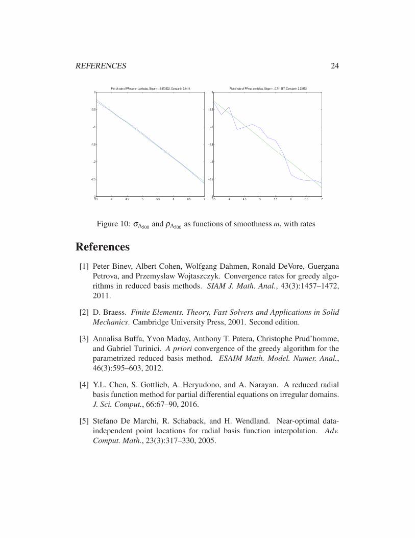
6.2 Observations for varying smoothness

We now check the behavior of the greedy method when the smoothness parameter

m of the Hilbert spaces W m2 (Rd) changes. In view of (22) and (23), and since

we saw before that the greedy method focuses on the differential operator and

the domain, not on boundary values, Figure 10 shows rates −0.67 and −0.71 as


−1

0

1

−1

0

10

0.02

0.04

0.06

PF2 on delta functionals for step 150

−1

0

1

−1

0

1

−5

0

5

10

x 10−3

Newton basis function for step 150

−1 0 1−1

−0.5

0

0.5

1Functional distribution

Figure 6: P2Λ500

(δx) on the domain, the basis function vµ150, and the selected 150

functionals, with the final selected domain functional marked with a blue asterisk

in the northwest, the contours being those of vµ150.

functions of m that confirm the −(m−3)/2 rate of (22) for both σΛ500and ρΛ500

as functions of m after 500 steps of the greedy method.

6.3 Use of Basis Functions

To get examples of solving specific Poisson problems via (20) using the basis ob-

tained by the Greedy Method, we selected a run for smoothness m = 6 to generate

the basis first, the other parameters being as in the previous examples. Then the

functions f and g of (1) were defined to let the true solution be of the form K(·,z)for a different kernel K and a point z = (−π/10,0). This allows to check cases

with solutions of different smoothness.

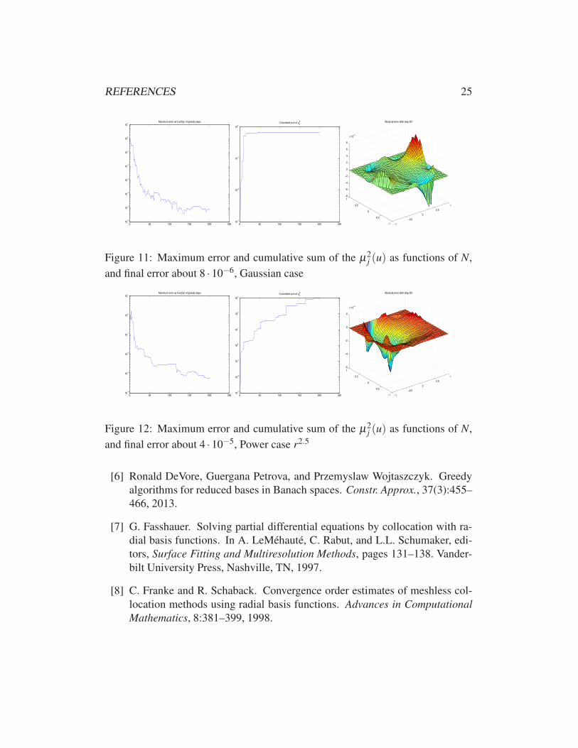
The first case is the infinitely smooth situation where K is a Gaussian. Figure

11 shows a very fast decay of the error, a fast increase of the cumulative sum of

the coefficients µ2j (u) from (20), and the final maximal error 8 · 10−6, roughly.

A less smooth solution is of the form r2.5 with r = ‖ · −z‖2 with a derivative

singularity at z, and the corresponding results are in Figure 12. The µ2j decay

much more slowly, and the solver has to fight with the derivative singularity at z.

The two cases were aligned by factors to start with an error of roughly one using

the same precalculated basis. Recall that classical Harmonic Analysis shows that

decay rates of coefficients of orthonormal expansions depend on smoothness and

determine convergence rates.


0 1 2 3 4 5 6 7−1.5

−1

−0.5

0

0.5

1

1.5

2

2.5

3

3.5Loglog plot of C

−1 norm, Rate = 0.688177, factor= 0.248363

0 1 2 3 4 5 6 7−2

0

2

4

6

8

10Loglog plot of C condition, Rate = 1.70018, factor= 0.229213

Figure 7: Norm and condition estimate of matrix C(N) as functions of N.

6.4 The Extended Greedy Method

The Extended Greedy Method from Section 4.3 was run in the same situations as

in Sections 6.1 and 6.2. The results are given from Figure 13 on.

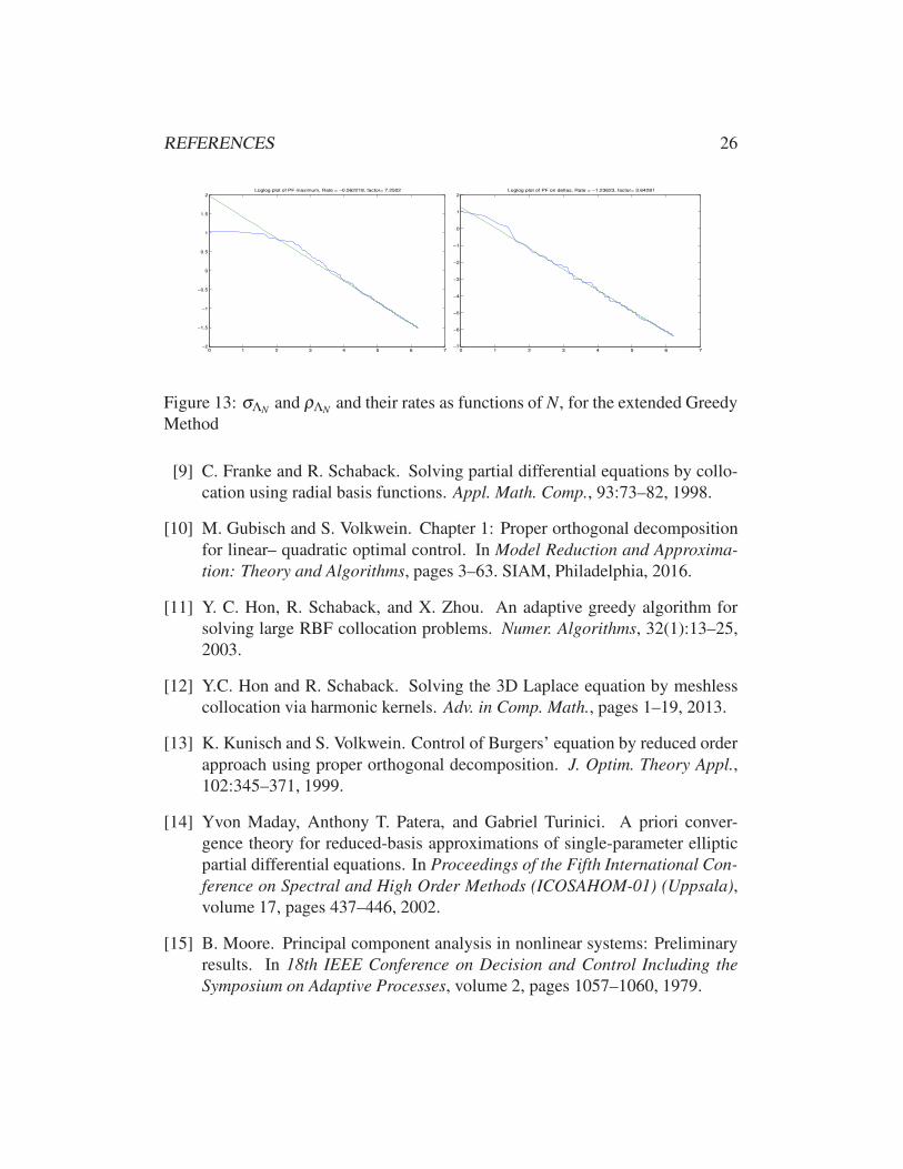
The rates in the left parts of Figures 1 and 13 are similar, but not in the right parts.

Since the extended method picks more boundary points than the original method,

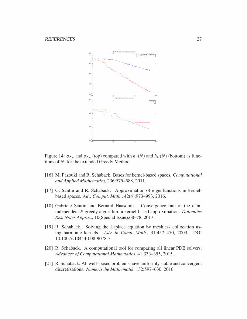
the convergence rate on the delta functionals is now much better. Similarly, Fig-

ures 2 and 14 differ considerably. The error in the interior decays much better,

and the fill distances in the domain and on the boundary show a better alignment.

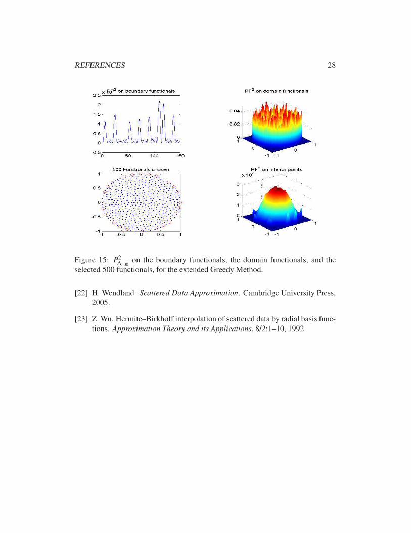
Figure 15 adds a plot of the Power Function on the domain to the three plots of

Figure 4, and it should be compared to Figure 5. One can see that the improved

selection of boundary functionals now avoids large values of the Power Function

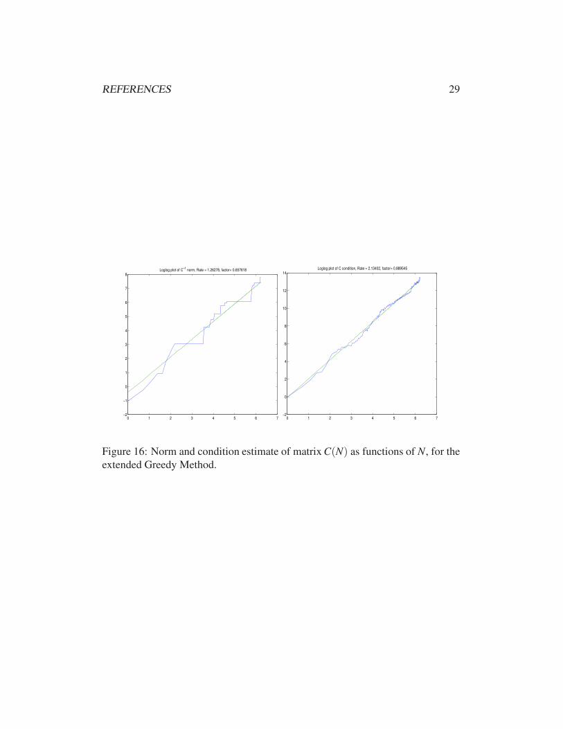
on the boundary. The other results are very similar, and plots are omitted, except

for the condition. The extended method is less stable, if Figures 7 and 16 are

compared.

From Lemma 2 one might hope that the extended Greedy Method performs better

as a function of smoothness, but this cannot be supported by experiments. The

rates for the situation corresponding to Figure 10 come out to be roughly -0.69

and -0.71, respectively, but the right-hand plot is much smoother. The actual plot

is suppressed.

7 SUMMARY AND OPEN PROBLEMS 22

0 1 2 3 4 5 6 7−12

−10

−8

−6

−4

−2

0

2

4

6Loglog plot of Singular values, Rate = −2.37812, factor= 186.785

Figure 8: Singular value decay of the matrix of suggested basis functions.

7 Summary and Open Problems

Roughly, the P-greedy method for solving Dirichlet problems for second-order el-

liptic operators in W m2 (Rd) seems to behave like the comparable P-greedy method

for interpolation of functions in W m−22 (Rd), with all its pros and cons. It focuses

on the domain, not on the boundary, and it tends to produce an asymptotically uni-

form distribution of evaluation points there, with an unexpectedly small number

of points for sampling the boundary values.

On the theoretical side, this opens the quest for a thorough analysis of Kolmogo-

roff N-widths for such PDE problems. A reasonable hypothesis is that these be-

have like those without differential operators, but for spaces of functions with

lower-order smoothness.

Another observation is that the maximum of the generalized Power Function taken

on all delta functionals, being a central quantity for pointwise error bounds, shows

the same asymptotics as the maximum of the generalized Power Function taken

on all chosen PDE data functionals. This is no surprise for well-posed problems,

7 SUMMARY AND OPEN PROBLEMS 23

0 1 2 3 4 5 6 7−10

−8

−6

−4

−2

0

2Loglog plot of RMSQ norms, Rate = −1.65707, factor= 4.28255

0 1 2 3 4 5 6 7−10

−8

−6

−4

−2

0

2Loglog plot of Sup norms, Rate = −1.44145, factor= 6.3255

Figure 9: RMSQ and Sup

but it opens a way for explicitly computable factors for error bounds in terms of

the Hilbert space norm of the true solution.

We supplied an Extended Greedy Method that cares for the delta functionals in a

better way, but it falls out of the Hilbert space foundation, so far. Its analysis is

another open problem.

Using the standard Hilbert space background [19, 12], we also can formulate a

P-greedy method for solving Dirichlet problems for harmonic functions in 2D or

3D. It will follow the Kolmogoroff N-width theory for such cases, but the latter

seems to be open.

There are other greedy techniques on the market (“ f –greedy” and “ f/P-greedy”)

that apply to specific problems of the form (1), not uniformly to the whole class.

But their convergence analysis is less far developed, see [18].

Acknowledgment

Special thanks go to Gabriele Santin for several helpful remarks.

REFERENCES 24

3.5 4 4.5 5 5.5 6 6.5 7−3

−2.5

−2

−1.5

−1

−0.5

0Plot of rate of PFmax on Lambdas, Slope = −0.673522, Constant= 2.1414

3.5 4 4.5 5 5.5 6 6.5 7−3

−2.5

−2

−1.5

−1

−0.5

0Plot of rate of PFmax on deltas, Slope = −0.711287, Constant= 2.23952

Figure 10: σΛ500and ρΛ500

as functions of smoothness m, with rates

References

[1] Peter Binev, Albert Cohen, Wolfgang Dahmen, Ronald DeVore, Guergana

Petrova, and Przemyslaw Wojtaszczyk. Convergence rates for greedy algo-

rithms in reduced basis methods. SIAM J. Math. Anal., 43(3):1457–1472,

2011.

[2] D. Braess. Finite Elements. Theory, Fast Solvers and Applications in Solid

Mechanics. Cambridge University Press, 2001. Second edition.

[3] Annalisa Buffa, Yvon Maday, Anthony T. Patera, Christophe Prud’homme,

and Gabriel Turinici. A priori convergence of the greedy algorithm for the

parametrized reduced basis method. ESAIM Math. Model. Numer. Anal.,

46(3):595–603, 2012.

[4] Y.L. Chen, S. Gottlieb, A. Heryudono, and A. Narayan. A reduced radial

basis function method for partial differential equations on irregular domains.

J. Sci. Comput., 66:67–90, 2016.

[5] Stefano De Marchi, R. Schaback, and H. Wendland. Near-optimal data-

independent point locations for radial basis function interpolation. Adv.

Comput. Math., 23(3):317–330, 2005.

REFERENCES 25

0 50 100 150 200 25010

−6

10−5

10−4

10−3

10−2

10−1

100

101

Maximum error as function of greedy steps

0 50 100 150 200 25010

−3

10−2

10−1

100

Cumulated sum of µk

2

−1

−0.5

0

0.5

1

−1

−0.5

0

0.5

1

−8

−6

−4

−2

0

2

4

6

8

x 10−6

Absolute error after step 201

Figure 11: Maximum error and cumulative sum of the µ2j (u) as functions of N,

and final error about 8 ·10−6, Gaussian case

0 50 100 150 200 25010

−4

10−3

10−2

10−1

100

101

Maximum error as function of greedy steps

0 50 100 150 200 25010

−3

10−2

10−1

100

101

102

103

Cumulated sum of µk

2

−1

−0.5

0

0.5

1

−1

−0.5

0

0.5

1

−6

−4

−2

0

2

x 10−4

Absolute error after step 201

Figure 12: Maximum error and cumulative sum of the µ2j (u) as functions of N,

and final error about 4 ·10−5, Power case r2.5

[6] Ronald DeVore, Guergana Petrova, and Przemyslaw Wojtaszczyk. Greedy

algorithms for reduced bases in Banach spaces. Constr. Approx., 37(3):455–

466, 2013.

[7] G. Fasshauer. Solving partial differential equations by collocation with ra-

dial basis functions. In A. LeMéhauté, C. Rabut, and L.L. Schumaker, edi-

tors, Surface Fitting and Multiresolution Methods, pages 131–138. Vander-

bilt University Press, Nashville, TN, 1997.

[8] C. Franke and R. Schaback. Convergence order estimates of meshless col-

location methods using radial basis functions. Advances in Computational

Mathematics, 8:381–399, 1998.

REFERENCES 26

0 1 2 3 4 5 6 7−2

−1.5

−1

−0.5

0

0.5

1

1.5

2Loglog plot of PF maximum, Rate = −0.562218, factor= 7.2502

0 1 2 3 4 5 6 7−7

−6

−5

−4

−3

−2

−1

0

1

2Loglog plot of PF on deltas, Rate = −1.23623, factor= 3.64281


and their rates as functions of N, for the extended Greedy

Method

[9] C. Franke and R. Schaback. Solving partial differential equations by collo-

cation using radial basis functions. Appl. Math. Comp., 93:73–82, 1998.

[10] M. Gubisch and S. Volkwein. Chapter 1: Proper orthogonal decomposition

for linear– quadratic optimal control. In Model Reduction and Approxima-

tion: Theory and Algorithms, pages 3–63. SIAM, Philadelphia, 2016.

[11] Y. C. Hon, R. Schaback, and X. Zhou. An adaptive greedy algorithm for

solving large RBF collocation problems. Numer. Algorithms, 32(1):13–25,

2003.

[12] Y.C. Hon and R. Schaback. Solving the 3D Laplace equation by meshless

collocation via harmonic kernels. Adv. in Comp. Math., pages 1–19, 2013.

[13] K. Kunisch and S. Volkwein. Control of Burgers’ equation by reduced order

approach using proper orthogonal decomposition. J. Optim. Theory Appl.,

102:345–371, 1999.

[14] Yvon Maday, Anthony T. Patera, and Gabriel Turinici. A priori conver-

gence theory for reduced-basis approximations of single-parameter elliptic

partial differential equations. In Proceedings of the Fifth International Con-

ference on Spectral and High Order Methods (ICOSAHOM-01) (Uppsala),

volume 17, pages 437–446, 2002.

[15] B. Moore. Principal component analysis in nonlinear systems: Preliminary

results. In 18th IEEE Conference on Decision and Control Including the

Symposium on Adaptive Processes, volume 2, pages 1057–1060, 1979.

REFERENCES 27

100

101

102

103

10−3

10−2

10−1

100

101

Both PF maxima as functions of N

PF on PDE functionalsPF on delta functionals

100

101

102

103

10−2

10−1

100

101

hB and h

D as functions of N

hB

hD


(top) compared with hΓ(N) and hΩ(N) (bottom) as func-

tions of N, for the extended Greedy Method.

[16] M. Pazouki and R. Schaback. Bases for kernel-based spaces. Computational

and Applied Mathematics, 236:575–588, 2011.

[17] G. Santin and R. Schaback. Approximation of eigenfunctions in kernel-

based spaces. Adv. Comput. Math., 42(4):973–993, 2016.

[18] Gabriele Santin and Bernard Haasdonk. Convergence rate of the data-

independent P-greedy algorithm in kernel-based approximation. Dolomites

Res. Notes Approx., 10(Special Issue):68–78, 2017.

[19] R. Schaback. Solving the Laplace equation by meshless collocation us-

ing harmonic kernels. Adv. in Comp. Math., 31:457–470, 2009. DOI

10.1007/s10444-008-9078-3.

[20] R. Schaback. A computational tool for comparing all linear PDE solvers.

Advances of Computational Mathematics, 41:333–355, 2015.

[21] R. Schaback. All well–posed problems have uniformly stable and convergent

discretizations. Numerische Mathematik, 132:597–630, 2016.

REFERENCES 28

Figure 15: P2Λ500

on the boundary functionals, the domain functionals, and the

selected 500 functionals, for the extended Greedy Method.

[22] H. Wendland. Scattered Data Approximation. Cambridge University Press,

2005.

[23] Z. Wu. Hermite–Birkhoff interpolation of scattered data by radial basis func-

tions. Approximation Theory and its Applications, 8/2:1–10, 1992.

REFERENCES 29

0 1 2 3 4 5 6 7−2

−1

0

1

2

3

4

5

6

7

8Loglog plot of C

−1 norm, Rate = 1.26278, factor= 0.657618

0 1 2 3 4 5 6 7−2

0

2

4

6

8

10

12

14Loglog plot of C condition, Rate = 2.13402, factor= 0.889545

Figure 16: Norm and condition estimate of matrix C(N) as functions of N, for the

extended Greedy Method.

A Greedy Method for Solving Classes of PDE...

Documents

Transcript of A Greedy Method for Solving Classes of PDE...