A Fixed-Point Operator for Inference inVariational Bayesian Latent Gaussian Models

Rishit Shethrishit.sheth@tufts.edu

Roni Khardonroni@cs.tufts.edu

Department of Computer Science, Tufts University, Medford, MA, USA

Abstract

Latent Gaussian Models (LGM) provide arich modeling framework with general infer-ence procedures. The variational approxima-tion offers an effective solution for such mod-els and has attracted a significant amountof interest. Recent work proposed a fixed-point (FP) update procedure to optimize thecovariance matrix in the variational solutionand demonstrated its efficacy in specific mod-els. The paper makes three contributions.First, it shows that the same approach canbe used more generally in extensions of LGM.Second, it provides an analysis identifyingconditions for the convergence of the FPmethod. Third, it provides an extensive ex-perimental evaluation in Gaussian processes,sparse Gaussian processes, and generalizedlinear models, with several non-conjugate ob-servation likelihoods, showing wide applica-bility of the FP method and a significant ad-vantage over gradient-based optimization.

1 INTRODUCTION

Latent Gaussian Models (LGM) provide a rich model-ing framework with general inference procedures andhave attracted a significant amount of interest. As ar-gued in previous work (Challis & Barber, 2013; Khanet al., 2013), LGM capture many existing models asspecial cases including Gaussian Processes (GP), gen-eralized linear models, probabilistic PCA, and more.With a small extension, LGM also capture the sparseGP model which enables efficient inference reducingthe cubic complexity of standard GP.

Appearing in Proceedings of the 19th International Con-ference on Artificial Intelligence and Statistics (AISTATS)2016, Cadiz, Spain. JMLR: W&CP volume 51. Copyright2016 by the authors.

The extended LGM model is specified by (1) belowwhere w ∈ Rd, f ∈ Rn, and the site potentials φi(fi)implicitly capture the non-Gaussian data likelihood.The distribution p(f |w) varies according to the model.

w ∼ N (µ,Σ), f |w ∼ p(f |w), p(data|f) =∏i

φi(fi),

(1)For example, in logistic regression w is the weight vec-tor, p(f |w) = δ(f−HTw) (where H = (h1, h2, . . . , hn)and hi is the ith example), and φi(fi) = σ(yifi) wherethe label yi is in {−1, 1}. Other linear models can bespecified by replacing the site potentials φi(fi) yieldingthe generalized linear model (GLM). For Gaussian pro-cesses with mean function m(·) and covariance K(·, ·),we have d = n, and w is the latent function at sam-ple points x yielding w ∼ N (m(x),K(x, xT )). Here wehave f = w, which for uniformity we write as p(f |w) =δ(f − HTw) with H = I, and φi(fi) = p(yi|fi) isthe likelihood of observations. In the sparse model, wrepresents the latent function at the pseudo inputs uand f is the latent function at x (Titsias, 2009). Inthis case p(f |w) is a linear conditional Gaussian andφi(fi) = p(yi|fi) (Sheth et al., 2015).

Since all these models include non-conjugate priors,computation of the posterior and marginal likelihoodare challenging and various approaches and approxi-mations have been developed. Among these, the vari-ational approach has been extensively investigated re-cently, as it provides a well justified criterion – max-imizing a lower bound on the marginal likelihood,known as the variational lower bound (VLB). In addi-tion, the variational approximation is computationallystable and yields good results in practice (Opper & Ar-chambeau, 2009; Titsias, 2009; Lazaro-gredilla & Tit-sias, 2011; Khan et al., 2012; Challis & Barber, 2013;Khan et al., 2013; Hensman et al., 2013; Khan, 2014;Titsias & Lazaro-gredilla, 2014; Gal et al., 2014; Hens-man et al., 2015; Sheth et al., 2015; Hoang et al., 2015).In this approach, a variational distribution

q(w, f) = q(w)p(f |w), where q(w) ∼ N (m, V ) (2)

A Fixed-Point Operator for Variational Inference in LGM

is used to approximate the posterior and (m, V ) arechosen to minimize the KL divergence to the true pos-terior. Thus the variational distribution is not in gen-eral form. It assumes a Gaussian distribution over wand uses an explicit form equating q(f |w) = p(f |w).

This optimization, especially optimizing V , is non triv-ial and several approaches have been proposed. In thecontext of GP with non-conjugate likelihoods, Opper& Archambeau (2009) observed that V has a specialstructure and proposed a re-parametrization that re-duces the number of parameters from O(n2) to O(n).The work of Khan et al. (2012) showed that this pa-rameterization is not concave and proposed a concaveimprovement for that algorithm. For LGM, Challis& Barber (2013) showed that for log-concave site po-tentials the variational lower bound is concave in mand the Cholesky factor of V and proposed gradientbased optimization. The work of (Khan et al., 2013;Khan, 2014) uses dual decomposition to obtain fasterinference. The sparse GP model was recently exploredby several groups. Here the objective was optimizedwith gradient search and the dual method of Khanet al. (2013) and was further developed for big datawith stochastic gradients and parallelization (Hens-man et al., 2013; Titsias & Lazaro-gredilla, 2014; Hens-man et al., 2015; Gal et al., 2014; Sheth et al., 2015).

This paper is motivated by recent proposals to use afixed point (FP) update, of the form V ← T (V ), forinference of the covariance function V in some spe-cial cases of LGM. In particular, Honkela et al. (2010)proposed FP as a heuristic to simplify the update fora Gaussian covariance within their adaptation of theconjugate gradient algorithm to use natural gradients,and Sheth et al. (2015) proposed a similar update inthe context of sparse GP. The work of Sheth et al.(2015) provided some empirical evidence that T (V )acts as a contraction in many cases and that it oftenleads to fast convergence of the sparse model. Butneither work provides an analysis of whether and un-der what conditions such an update is guaranteed toconverge. Similarly we are not aware of any system-atic investigation of the convergence of FP in practiceacross different models and site potentials.

This paper makes three contributions. The first is inobserving that the FP algorithm is more widely appli-cable and that it can be used in the extended LGMmodel. The second contribution is an analysis provid-ing sufficient conditions for convergence of the updateoperator T (V ) and showing that the convergence con-ditions hold for many instances of that model. Theconditions for convergence rely only on properties ofthe site potential functions and can be tested in ad-vance for any concrete model. The third contributionis an experimental evaluation in GP, sparse GP, and

GLM for several likelihood functions showing that theFP method is widely applicable and that it offers sig-nificant advantages in convergence time over gradientbased methods across all these models.

2 FIXED POINT UPDATES

In this section we review the variational approach tothe extended LGM and the resulting FP update. Mostof the development in this section is either directlystated or is implicit in previous work (Challis & Bar-ber, 2013; Sheth et al., 2015). But the characterizationof the marginal variances in (4) and corresponding im-plication of applicability in LGM did not previouslyappear in this form.

Starting with the model in (1) we can apply the varia-tional distribution (2) to yield the following standardVLB:

log p(data)

= log

∫N (w|µ,Σ)p(f |w)

∏i

φi(fi)dfdw

≥∫q(w, f) log

(N (w|µ,Σ)p(f |w)

q(w, f)

∏i

φi(fi)

)dfdw

=∑i

Eq(w,f)[log φi(fi)]− dKL(q(w)‖N (w|µ,Σ))

=∑i

Eq(fi)[log φi(fi)]− dKL(q(w)‖N (w|µ,Σ)) (3)

where dKL is the Kullback-Leibler divergence. Below,we refer to the bound given in (3) as the VLB. Notethat p(f |w) does not affect the dKL term and it affectsthe first term only through the marginal distributionq(fi). In this paper we focus on cases where q(fi) isGaussian, which holds for the models mentioned in theintroduction. However, FP for the extended LGM canbe used with other forms of p(f |w) as long as expecta-tions and derivatives w.r.t. q(fi), as identified below,are available or can be estimated.

Optimizing the VLB w.r.t. m is stable and can be doneeffectively with Newton’s method or BFGS and thederivatives are given in previous work. In the followingwe focus on the optimization w.r.t. V .

To proceed, we need explicit expressions for q(fi).In the cases where f = HTw, we have fi = hTi wand as a result mqi = hTi m, and vqi = hTi V hi.For sparse GP, we recall that w represents the la-tent function at the pseudo inputs u and f is thelatent function at x. We therefore have that f |w ∼N (mx+KxuK

−1uu (w−mu),Kxx−KxuK

−1uuKux) where

we follow standard notation representing the argu-ments of m(·) and K(·, ·) using subscripts. Now, us-ing q(w) = N (m, V ) and marginalizing we obtain

Sheth, Khardon

mqi = mxi + KiuK−1uu (m − mu) and vqi = Kii +

KiuK−1uu (V −Kuu)K−1uuKui. The important point for

our analysis is that in all these cases vqi is a sum of ascalar and a quadratic form in V and can be capturedabstractly using

vqi(V ) = ci + dTi V di (4)

where we emphasize the dependence on V . For the

derivative of the VLB note that∂Eq(fi)

[log φi(fi)]

∂V =∂Eq(fi)

[log φi(fi)]

∂vqi

∂vqi∂V and that

∂vqi∂V = did

Ti = Di is a

rank 1 positive semi-definite (PSD) matrix. Combin-ing this with derivatives for dKL, we can get two al-ternative expressions for the derivatives, showing that

∂VLB

∂V=

1

2V −1 − 1

2Σ−1 − 1

2

∑i

γi(vqi)Di (5)

where γi(mqi , vqi) = −2∂Eq(fi)

[log φi(fi)]

∂vqi=

EN (fi|mqi,vqi )

[− ∂2

∂f2i

log φi(fi)] = (6)

EN (fi|mqi,vqi )

[−((f−mqi

)2

vqi− 1) 1

vqilog φi(fi)] (7)

and where (6) derived by Sheth et al. (2015) shows thatγi > 0 for log concave site potentials and (7) derivedby Challis & Barber (2013) can be used in cases wherelog φi(fi) is not differentiable but the expectation isdifferentiable.

The derivative (5) immediately suggests the FP up-date

T (V ) = (Σ−1 +∑i

γi(vqi)Di)−1 (8)

The expression for γi is a function of the marginal vari-ational distribution q(mqi , vqi) and the generic site po-tentials used, and can be calculated and viewed as afunction of the parameters mqi , vqi . Below we refer tothis function abstractly as γ(m, v) and study the con-vergence of the proposed method based on propertiesof this function.

3 ANALYSIS

We start by noting basic properties of the FP update.For any fixed m, let V ∗ be the optimizer of the VLBw.r.t m.

Proposition 1 (1) V ∗ = T (V ∗), (2) V = T (V ) im-

plies that ∂VLB∂V |V = 0, (3) ∂VLB

∂V |V = 0 and V is full

rank implies V = V ∗.

Proof: From (5), (8) we obviously have:

∂VLB

∂V=

1

2(V −1 − T (V )−1) (9)

This shows that the optimal covariance V ∗, where thederivative is zero, is a fixed-point of T (V ). In addi-tion, the equation implies that if the FP method con-

verges and T (V ) = V then ∂VLB∂V = 0 and we have

reached a stationary point. Finally, it can be shown

that ∂VLB∂L L−1 = 2∂VLB

∂V where L is the Choleskyfactor of V = LLT . Now, since for log-concave sitepotentials the VLB is concave in L (Challis & Barber,2013) we see that if the FP method converges to Vand V is full rank then V = V ∗.

The proposition shows that the fixed point of T () iden-tifies V ∗. We note that a unique optimum does notimply that the VLB is concave in V . Next, we de-fine sufficient conditions that guarantee that repeatedapplication of T () does converge:

Condition 1: for all m, v, γ(m, v) ≥ 0.Condition 2a: for all fixed values of m, γ(m, v) ismonotonically non-decreasing in v.Condition 2b: for all fixed values of m, γ(m, v) ismonotonically non-inccreasing in v.

Theorem 1 (1) If conditions 1 and 2a hold then theFP update converges to V ∗ or to a limit cycle of sizetwo. (2) If conditions 1 and 2b hold then the FP updateconverges to V ∗.

Proof: For matrices A,B we denote A � 0 when Ais PSD and say that B � A if B −A � 0. Now, usingCondition 1 and (8) we see that for any V , we haveT (V )−1 � Σ−1 implying that

∀V, T (V ) � Σ (10)

and in particular T (V ∗) � Σ.

Next observe from (4) that for any A � B, we havevqi(A) ≥ vqi(B), and from Condition 2a this impliesγi(vqi(A)) ≥ γi(vqi(B)). Therefore, from (8), we have

∀A,B s.t. A � B, T (A) � T (B) (11)

Applying (11) to V ∗ � Σ, and using (10) to add Σ asan upper bound we get

T (Σ) � V ∗ � Σ (12)

Now, repeatedly applying (11) to the sequence andusing (10) to add Σ as an upper bound gives

T (Σ)�T 3(Σ)� . . .�V ∗� . . .�T 4(Σ)�T 2(Σ)�Σ(13)

Denote γ`i = γ(vqi(T`(Σ))) and γ∗i = γi(vqi(V

∗)).Then Condition 2a and (13) imply

γ1i ≤ γ3i ≤ . . . ≤ γ∗i ≤ . . . ≤ γ4i ≤ γ2i ≤ γ0i (14)

A Fixed-Point Operator for Variational Inference in LGM

vi

mi

sign[ −∂λi / ∂v

i ] for Logistic likelihood

0 20 40 60 80 100−20

−15

−10

−5

0

5

10

15

20

−1

1

(a)

vi

mi

sign[ −∂λi / ∂v

i ] for Logistic likelihood

0 1 2 3 4 5−2

−1.5

−1

−0.5

0

0.5

1

1.5

2

−1

1

(b)

vi

mi

sign[ −∂λi / ∂v

i ] for Logistic likelihood

0 1 2 3 4 5−2

−1.5

−1

−0.5

0

0.5

1

1.5

2

−1

1

(c)

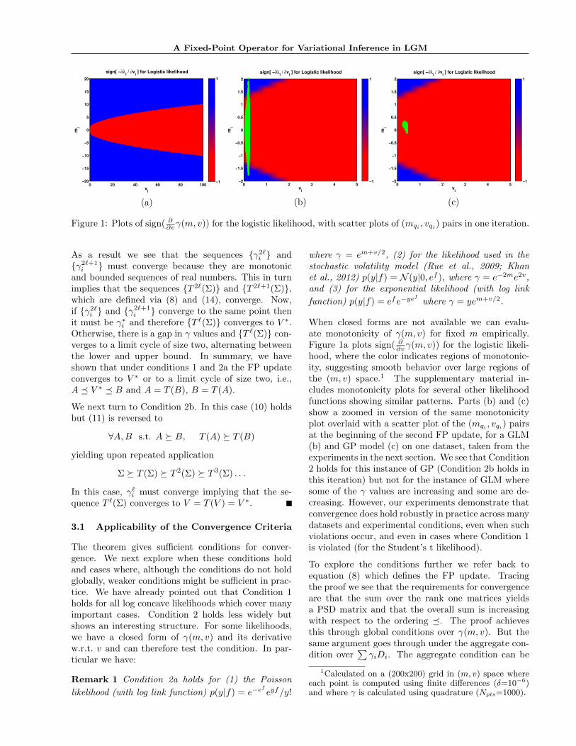
Figure 1: Plots of sign( ∂∂vγ(m, v)) for the logistic likelihood, with scatter plots of (mqi , vqi) pairs in one iteration.

As a result we see that the sequences {γ2`i } and{γ2`+1i } must converge because they are monotonic

and bounded sequences of real numbers. This in turnimplies that the sequences {T 2`(Σ)} and {T 2`+1(Σ)},which are defined via (8) and (14), converge. Now,if {γ2`i } and {γ2`+1

i } converge to the same point thenit must be γ∗i and therefore {T `(Σ)} converges to V ∗.Otherwise, there is a gap in γ values and {T `(Σ)} con-verges to a limit cycle of size two, alternating betweenthe lower and upper bound. In summary, we haveshown that under conditions 1 and 2a the FP updateconverges to V ∗ or to a limit cycle of size two, i.e.,A � V ∗ � B and A = T (B), B = T (A).

We next turn to Condition 2b. In this case (10) holdsbut (11) is reversed to

∀A,B s.t. A � B, T (A) � T (B)

yielding upon repeated application

Σ � T (Σ) � T 2(Σ) � T 3(Σ) . . .

In this case, γ`i must converge implying that the se-quence T `(Σ) converges to V = T (V ) = V ∗.

3.1 Applicability of the Convergence Criteria

The theorem gives sufficient conditions for conver-gence. We next explore when these conditions holdand cases where, although the conditions do not holdglobally, weaker conditions might be sufficient in prac-tice. We have already pointed out that Condition 1holds for all log concave likelihoods which cover manyimportant cases. Condition 2 holds less widely butshows an interesting structure. For some likelihoods,we have a closed form of γ(m, v) and its derivativew.r.t. v and can therefore test the condition. In par-ticular we have:

Remark 1 Condition 2a holds for (1) the Poisson

likelihood (with log link function) p(y|f) = e−ef

eyf/y!

where γ = em+v/2, (2) for the likelihood used in thestochastic volatility model (Rue et al., 2009; Khanet al., 2012) p(y|f) = N (y|0, ef ), where γ = e−2me2v,and (3) for the exponential likelihood (with log link

function) p(y|f) = efe−yef

where γ = yem+v/2.

When closed forms are not available we can evalu-ate monotonicity of γ(m, v) for fixed m empirically.Figure 1a plots sign( ∂∂vγ(m, v)) for the logistic likeli-hood, where the color indicates regions of monotonic-ity, suggesting smooth behavior over large regions ofthe (m, v) space.1 The supplementary material in-cludes monotonicity plots for several other likelihoodfunctions showing similar patterns. Parts (b) and (c)show a zoomed in version of the same monotonicityplot overlaid with a scatter plot of the (mqi , vqi) pairsat the beginning of the second FP update, for a GLM(b) and GP model (c) on one dataset, taken from theexperiments in the next section. We see that Condition2 holds for this instance of GP (Condition 2b holds inthis iteration) but not for the instance of GLM wheresome of the γ values are increasing and some are de-creasing. However, our experiments demonstrate thatconvergence does hold robustly in practice across manydatasets and experimental conditions, even when suchviolations occur, and even in cases where Condition 1is violated (for the Student’s t likelihood).

To explore the conditions further we refer back toequation (8) which defines the FP update. Tracingthe proof we see that the requirements for convergenceare that the sum over the rank one matrices yieldsa PSD matrix and that the overall sum is increasingwith respect to the ordering �. The proof achievesthis through global conditions over γ(m, v). But thesame argument goes through under the aggregate con-dition over

∑γiDi. The aggregate condition can be

1Calculated on a (200x200) grid in (m, v) space whereeach point is computed using finite differences (δ=10−6)and where γ is calculated using quadrature (Npts=1000).

Sheth, Khardon

abstracted as a less stringent sufficient condition forconvergence, but it is difficult to formalize it in a com-pact and crisp manner, and we have therefore optedfor the global conditions above.

One can easily adjust the FP algorithm to detect vio-lations of these conditions and use a modified update.For condition 1, our implementation replaces γi with0 whenever it is negative thus maintaining the PSDcondition. For violations of condition 2, one could re-sort to standard gradient update whenever this occurs,for example in the case illustrated for GLM. However,our experimental comparison suggests that FP is sig-nificantly faster than standard gradients and thereforethis will likely yield an inferior performance.

3.2 Discussion: FP and Gradient Search

We next show that the FP method is closely relatedto gradient search with a fixed step size, giving twosuch interpretations. For the first, recall the relationbetween the gradient and T () expressed in (9) andrewrite T () and (9) in terms of the precision matrixQ = V −1 so that Q is updated to T (Q). We have

∂VLB

∂Q−1=

1

2(Q− T (Q)) (15)

T (Q) = Q− 2∂VLB

∂Q−1(16)

As (16) shows, T (Q) takes a descent step w.r.t. thegradient of the inverse instead of an ascent step w.r.t.standard gradient. Thus the FP method can be seen asan unusual gradient method with a specific step size.

The second observation (first pointed out by an anony-mous reviewer) is that the FP update is a naturalgradient update with step size 1. Natural gradients(Amari & Nagaoka, 2000) adapt to the geometry ofthe optimized function and have been demonstrated toconverge faster than standard gradients in some cases.The natural gradient is a result of pre-multiplying thestandard gradient by the inverse of the Fisher infor-mation matrix I. Recall that exponential family dis-tributions can be alternatively described using theirnatural parameter θ or mean parameter η. As shownby (Sato, 2001; Hensman et al., 2012; Hoffman et al.,2013) the natural gradient with respect to θ can bederived using standard gradients with respect to η. Inparticular, using ∂N to denote the natural gradient, wehave ∂Nf

∂θ = I−1 ∂f∂θ = ∂f∂η . The corresponding natural

gradient update with step size 1 is θnew ← θold + ∂f∂η .

In our case, θ = (r, S) = (V −1m, 12V−1) and η =

(h,H) = (m,−(V + mmT )) and the update for Syields 1

2V−1 = 1

2 (Σ−1 +∑i γi(vqi)Di) which is iden-

tical to the FP update. The supplementary material

reviews these facts, and shows in addition that theanalysis applies whenever q(w) and p(w) are in thesame exponential family and a “FP-like” update canbe derived as a natural gradient with step size 1. Thisalso holds for the natural gradient of r which yields acorresponding FP update for m.

It is known (Hoffman et al., 2013; Sato, 2001) that insome cases (exponential family likelihoods with conju-gate priors and conjugate complete conditionals) size 1natural gradients are equivalent to coordinate ascentoptimization and they therefore converge. However,to our knowledge no existing prior analysis implies theconvergence of the FP update as proved above. Specif-ically, the conditions required by (Hoffman et al., 2013;Sato, 2001) do not hold for the extended LGM. More-over, exploratory experiments (provided in the supple-mentary material) show that applying the same typeof “FP-like” update to m is not generally stable andcan converge to an inferior local maximum, illustrat-ing that no such general conditions hold. Therefore,our analysis can be seen to identify specific conditionsunder which size 1 natural gradients lead to conver-gence. It would be interesting to explore more generalconditions under which convergence holds.

4 EXPERIMENTS

To show wide applicability, we evaluate the FP methodacross several probabilistic models and likelihood func-tions. In particular, we evaluate FP on GLM, GP,and sparse GP. We compare the performance of FP tothe gradient based optimization of Challis & Barber(2013) which we denote below by GRAD. Since we aremainly concerned with the optimization and its speed,the criterion in our comparison is the value of the VLBobtained by the methods as a function of time.

Our experiments include the Poisson likelihood whichsatisfies Conditions 1 and 2a, the Laplace and logisticlikelihoods which satisfy Condition 1 but not 2, andthe Student’s t likelihood which violates both condi-tions. In the latter case, we modify the implemen-tation so that whenever Condition 1 is violated, i.e.,γi < 0, it is set to zero. This heuristic ensures thepositive-definiteness of the variational covariance forall fixed point iterations. Thus we test if convergenceholds even when the conditions are not satisfied.

For all experiments we used the vgai package (Challis& Barber, 2011) that implements the GRAD method(Challis & Barber, 2013). GRAD optimizes the meanand Cholesky decomposition of the covariance jointlywith L-BFGS. To facilitate as close a comparison aspossible, the implementation of the fixed point meth-ods uses vgai as well but replaces the optimizationfunction call with the corresponding updates. The op-

A Fixed-Point Operator for Variational Inference in LGM

0 10 20 30 40 50 60 70 80 90 1001

1.5

2

2.5

3

3.5

4

4.5

5

5.5

6x 10

4

CPU Time (sec)

Ob

jecti

ve F

un

cti

on

Valu

eGLM−Logistic on a9a (32561, 123)

0 2000 4000 6000 8000 10000 120000.9

1

1.1

1.2

1.3

1.4

1.5

1.6

1.7x 10

4

CPU Time (sec)

Ob

jec

tiv

e F

un

cti

on

Va

lue

glm−logistic on epsilon (15000, 1000)

0 5 10 15 20 25 30 35 40 45 500

0.5

1

1.5

2

2.5

3x 10

4

CPU Time (sec)

Ob

jecti

ve F

un

cti

on

Valu

e

glm−logistic on madelon (2600, 500)

0 0.1 0.2 0.3 0.4 0.5 0.6 0.7 0.8 0.9 1−8

−7

−6

−5

−4

−3

−2

−1

0

1x 10

4

CPU Time (sec)

Ob

jec

tiv

e F

un

cti

on

Va

lue

GLM−Poisson on ucsdpeds (4000, 30)

0 100 200 300 400 500 600 700 800 900 10000.4

0.6

0.8

1

1.2

1.4

1.6x 10

4

CPU Time (sec)

Ob

jec

tiv

e F

un

cti

on

Va

lue

GLM−Poisson on epsilon−count (15000,500)

0 0.05 0.1 0.15 0.2 0.25 0.3 0.35 0.4−6

−5

−4

−3

−2

−1

0

1x 10

4

CPU Time (sec)

Ob

jecti

ve F

un

cti

on

Valu

e

GLM−Poisson on abalone (4177, 9)

0 5 10 15 20 252

2.5

3

3.5

4

4.5

5

5.5

6

6.5x 10

4

CPU Time (sec)

Ob

jecti

ve F

un

cti

on

Valu

e

glm−laplace on cahousing (20640, 8)

0 50 100 150 200 250 300 350 400 450 5000.5

1

1.5

2

2.5

3

3.5

4x 10

5

CPU Time (sec)

Ob

jecti

ve F

un

cti

on

Valu

e

glm−laplace on yearpred (51609, 90)

0 500 1000 15000

0.5

1

1.5

2

2.5

3x 10

5

CPU Time (sec)

Ob

jec

tiv

e F

un

cti

on

Va

lue

glm−laplace on wlan−long (19085, 466)

Figure 2: Evaluation for GLM showing objective function values with respect to training time. Numbers inparentheses in title refer to number of samples and dimensions of dataset. Legend for plots: GRAD (—), FPb(—). FPi (- -),

timization parameters for all algorithms were set tothe same values where applicable (see supplementarymaterial). Our experiments include two variants ofthe FP method. The first, as in the analysis, alter-nates between optimizing m and V where m is op-timized using Newton’s method and V is optimizedwith FP updates. This was the method recommendedby Sheth et al. (2015). We have found, however, thatcomplete optimization of m during the early iterationscan be expensive, and have therefore implemented asecond variant, closer to the simultaneous optimiza-tion of (m, V ) performed in GRAD. In particular, thealgorithm alternates between taking one gradient stepfor m using Newton’s method, and one fixed-point up-date T (V ). When m has converged we get fixed pointiterations on V and similarly if V has converged we

get second-order optimization on m. To distinguishthe methods we refer to them below as FPbatch (FPb)and FPincremental (FPi).

In our experiments we have observed the cycling be-havior suggested by the analysis in intermediate it-erations of FPb (see supplementary material). Note,however, that even if this occurs, once m is updated inthe next iteration the fixed point update for V is ableto exit this condition. Empirically, in all our experi-ments FPb and FPi do approach the optimal VLB.

The supplementary material includes a list of alldatasets used in the experiments. Briefly, we selectedmedium size datasets to start with and added largeones to demonstrate performance in GLM. We usedZ-score normalization for all features in all datasets.

Sheth, Khardon

0 10 20 30 40 50 60 70 80 90 1004

6

8

10

12

14

16

18

20

22

CPU Time (sec)

log

(O

bje

cti

ve F

un

cti

on

Valu

e)

GP−Logistic on a9a (500, 123)

0 10 20 30 40 50 60 70 80 90 1004

5

6

7

8

9

10

11

12

CPU Time (sec)

log

(O

bje

cti

ve F

un

cti

on

Valu

e)

GP−Logistic on musk (500, 166)

0 5 10 15 20 25 30 35 40 454

6

8

10

12

14

16

18

CPU Time (sec)

log

(O

bje

cti

ve F

un

cti

on

Valu

e)

GP−Logistic on usps (500, 256)

0 10 20 30 40 50 60 70 80 90 1008

10

12

14

16

18

20

22

24

CPU Time (sec)

log

(O

bje

cti

ve F

un

cti

on

Valu

e)

GP−Poisson on ucsdpeds (500, 30)

0 20 40 60 80 100 120 140 160 180 2005

10

15

20

25

30

CPU Time (sec)

log

(O

bje

cti

ve F

un

cti

on

Valu

e)

GP−Poisson on flares (500, 24)

0 5 10 15 20 25 30 35 40 45 508

10

12

14

16

18

20

22

24

26

CPU Time (sec)

log

(O

bje

cti

ve

Fu

nc

tio

n V

alu

e)

GP−Poisson on abalone (500, 9)

0 5 10 15 20 25 306

8

10

12

14

16

18

20

CPU Time (sec)

log

(O

bje

cti

ve

Fu

nc

tio

n V

alu

e)

GP−Laplace on cpusmall (500, 12)

0 10 20 30 40 50 60 70 80 90 1006

7

8

9

10

11

12

13

14

15

16

CPU Time (sec)

log

(O

bje

cti

ve F

un

cti

on

Valu

e)

GP−Laplace on spacega (500, 6)

0 5 10 15 20 25 30 35 40 45 5018.4253

18.4254

18.4254

18.4255

18.4255

18.4256

18.4256

18.4257

18.4257

CPU Time (sec)

log

(Obj

ectiv

e F

unct

ion

Val

ue)

GP−Laplace on cahousing (500, 8)

Figure 3: Evaluation for GP. See Figure 2 for description and legend.

The experimental setting is as follows. For GLM,Σ = 0.1I in all cases except flares where Σ = 0.001I.For GP and sparse GP, we use a zero mean prior andΣ is the corresponding kernel matrix, where we usethe Gaussian RBF kernel with length scale and scalefactor estimated from 200 randomly chosen samples(using the GPML toolbox (Rasmussen & Nickisch,2013)). The variance of the Laplace likelihood wasalso estimated in this way. The logistic and Poissonlikelihoods do not have parameters. The parametersof the Student’s t likelihood were fixed to ν = 3 andσ2 = 1

3 . Since our focus is on the optimization pro-cedure, hyperparameters remain fixed during the ex-periments and equal across the algorithms. Datasetsfor the GP experiment were sub-sampled to 500 sam-ples. The inducing set for the sparse GP experimentwas 100 samples randomly chosen and fixed across al-gorithms. The initial conditions for the optimization

were set to m = 0 and V = I, except in the caseof count data (where the log link function is sensitivew.r.t. numerical stability) where V = 0.1I.

Note that we test several probabilistic models andseveral likelihoods under the same algorithmic setupfor FP. This provides a robust evaluation of the FPmethod showing that it works well across all thesecases without specific adjustment for each case.

Figure 2 shows results of experiments with GLM acrossclassification, count regression and robust regression.The plots show a significant advantage of FPi in allcases, with GRAD reducing VLB well initially butslowing considerably thereafter in many cases. Pre-liminary experiments with smaller datasets (see sup-plementary material) showed the FP was competitivewith GRAD on the GLM model but did not show a sig-nificant difference. This shows that the advantage of

A Fixed-Point Operator for Variational Inference in LGM

0 500 1000 15002

3

4

5

6

7

8

9

10

11x 10

4

CPU Time (sec)

Ob

jec

tiv

e F

un

cti

on

Va

lue

Sparse GP−Laplace on cpusmall (100, 8192, 12)

0 50 100 150 200 250 300 350 400 450 500−2

0

2

4

6

8

10x 10

4

CPU Time (sec)

Ob

jecti

ve F

un

cti

on

Valu

e

Sparse GP−Laplace on spacega (100, 3106, 6)

0 1000 2000 3000 4000 5000 6000 7000 8000 9000 100002.35

2.4

2.45

2.5x 10

5

CPU Time (sec)

Obj

ectiv

e F

unct

ion

Val

ue

Sparse GP−Laplace on cahousing (100, 20640, 8)

Figure 4: Evaluation for sparse GP with Laplace likelihood. See Figure 2 for legend.

0 5 10 15 20 258

9

10

11

12

13

14

15

CPU Time (sec)

log

(O

bje

cti

ve

Fu

nc

tio

n V

alu

e)

GP−Student−T on cpusmall (500, 12)

0 10 20 30 40 50 60 70 80 90 1004

6

8

10

12

14

16

CPU Time (sec)

log

(O

bje

cti

ve F

un

cti

on

Valu

e)

GP−Student−T on spacega (500, 6)

0 20 40 60 80 100 120 140 160 180 20010

10.1

10.2

10.3

10.4

10.5

10.6

10.7

10.8

10.9

11

CPU Time (sec)

log

(O

bje

cti

ve F

un

cti

on

Valu

e)

GP−Student−T on cahousing (500, 8)

Figure 5: Evaluation for GP with (non-log-concave) Student’s t likelihood. See Figure 2 for legend.

the FP method is more pronounced for larger datasets.

Figure 3 shows results of experiments with GP on thesame likelihoods where both FP methods have a signif-icant advantage over GRAD and where the differencesare more dramatic than in GLM.

The FP method for the sparse GP model has alreadybeen evaluated with Poisson, logistic, and ordinal like-lihoods (Sheth et al., 2015). Figure 4 complements thisand shows the results of experiments with sparse GPfor the Laplace likelihood. We observe the same gen-eral behavior as in the full GP model with FPi beingthe fastest and GRAD and FPb being slower.

Figure 5 shows results of experiments with GP withthe Student’s t likelihood. In this case both conditions1 and 2 from our analysis do not hold. Nonetheless,the methods behave quite similarly in this case as well.

5 CONCLUSIONS

The paper shows that the FP method is applicable inthe extended LGM model, provides an analysis thatestablishes the convergences of the FP method andprovides an extensive experimental evaluation demon-strating that the FP method is applicable across GP,sparse GP, and GLM, that it converges for various like-lihood functions, and that it significantly outperforms

gradient based optimization in all these models.

We conclude with two directions for future work. Asmentioned above, this paper focused on the case wherep(f |w) is linear Gaussian but the same approach is ap-plicable as long as q(fi) and quantities relative to thisdistribution are efficiently computable. Probabilisticmatrix factorization (Salakhutdinov & Mnih, 2008) isa LGM where p(f |w) is more complex and where vari-ational solutions have been investigated (Lim & Teh,2007; Seeger & Bouchard, 2012). It would be inter-esting to develop efficient FP updates for this model.Along a different dimension, recent work on variationalinference has demonstrated the utility of stochasticgradient optimization (SG), with or without naturalgradients, for scalability to very large datasets. SGtypically requires careful control of decreasing learn-ing rates, whereas the FP method was shown to be re-lated to gradient step with a fixed step size. It wouldbe interesting to develop algorithms that combine thebenefits of both methods, by incorporating FP updateswithin SG.

Acknowledgments

Some of the experiments in this paper were performedon the Tufts Linux Research Cluster supported byTufts Technology Services.

Sheth, Khardon

References

Amari, S. and Nagaoka, H. Methods of InformationGeometry, volume 191 of Translations of Mathemat-ical monographs. Oxford University Press, 2000.

Challis, Edward and Barber, David. vgai softwarepackage, 2011. mloss.org/software/view/308/.

Challis, Edward and Barber, David. GaussianKullback-Leibler Approximate Inference. Journal ofMachine Learning Research, 14:2239–2286, 2013.

Gal, Yarin, van der Wilk, Mark, and Rasmussen, Carl.Distributed Variational Inference in Sparse Gaus-sian Process Regression and Latent Variable Mod-els. In Advances in Neural Information ProcessingSystems 27, pp. 3257–3265. 2014.

Hensman, James, Rattray, Magnus, and Lawrence,Neil D. Fast Variational Inference in the ConjugateExponential Family. In Advances in Neural Infor-mation Processing Systems 25, pp. 2888–2896. 2012.

Hensman, James, Fusi, Nicolo, and Lawrence, Neil D.Gaussian Processes for Big Data. In Proceedingsof the 29th Conference on Uncertainty in ArtificialIntelligence, pp. 282–290, 2013.

Hensman, James, Matthews, Alexander, and Ghahra-mani, Zoubin. Scalable Variational Gaussian Pro-cess Classification. In Proceedings of the 18th In-ternational Conference on Artificial Intelligence andStatistics, pp. 351–360, 2015.

Hoang, Trong Nghia, Hoang, Quang Minh, and Low,Bryan Kian Hsiang. A Unifying Framework of Any-time Sparse Gaussian Process Regression Modelswith Stochastic Variational Inference for Big Data.In Proceedings of the 32nd International Conferenceon Machine Learning, pp. 569–578, 2015.

Hoffman, Matthew D., Blei, David M., Wang, Chong,and Paisley, John William. Stochastic VariationalInference. Journal of Machine Learning Research,14(1):1303–1347, 2013.

Honkela, Antti, Raiko, Tapani, Kuusela, Mikael,Tornio, Matti, and Karhunen, Juha. Approxi-mate Riemannian Conjugate Gradient Learning forFixed-Form Variational Bayes. Journal of MachineLearning Research, 11:3235–3268, 2010.

Khan, Mohammad E. Decoupled Variational Gaus-sian Inference. In Advances in Neural InformationProcessing Systems 27, pp. 1547–1555, 2014.

Khan, Mohammad E., Mohamed, Shakir, and Murphy,Kevin P. Fast Bayesian Inference for Non-ConjugateGaussian Process Regression. In Advances in NeuralInformation Processing Systems 25, pp. 3149–3157.2012.

Khan, Mohammad E., Aravkin, Aleksandr Y., Fried-lander, Michael P., and Seeger, Matthias. Fast DualVariational Inference for Non-Conjugate LGMs. InProceedings of the 30th International Conference onMachine Learning, pp. 951–959, 2013.

Lazaro-gredilla, Miguel and Titsias, Michalis K. Varia-tional Heteroscedastic Gaussian Process Regression.In Proceedings of the 28th International Conferenceon Machine Learning, pp. 841–848, 2011.

Lim, Y. J. and Teh, Y. W. Variational Bayesian Ap-proach to Movie Rating Prediction. In Proceedingsof KDD Cup and Workshop, 2007.

Opper, Manfred and Archambeau, Cedric. The Vari-ational Gaussian Approximation Revisited. NeuralComputation, 21(3):786–792, 2009.

Rasmussen, Carl Edward and Nickisch, Hannes.GPML software package, 2013. http://www.

gaussianprocess.org/gpml/code/matlab/doc/.

Rue, Havard, Martino, Sara, and Chopin, Nicolas. Ap-proximate Bayesian Inference for Latent GaussianModels by using Integrated Nested Laplace Approx-imations. Journal of the Royal Statistical Society:Series B (Statistical Methodology), 71(2):319–392,2009.

Salakhutdinov, Ruslan and Mnih, Andriy. BayesianProbabilistic Matrix Factorization using MarkovChain Monte Carlo. In Proceedings of the 25th Inter-national Conference on Machine Learning, pp. 880–887, 2008.

Sato, Masa-aki. Online Model Selection Based on theVariational Bayes. Neural Computation, 13(7):1649–1681, 2001.

Seeger, Matthias W. and Bouchard, Guillaume. FastVariational Bayesian Inference for Non-ConjugateMatrix Factorization Models. In Proceedings of the15th International Conference on Artificial Intelli-gence and Statistics, pp. 1012–1018, 2012.

Sheth, Rishit, Wang, Yuyang, and Khardon, Roni.Sparse Variational Inference for Generalized Gaus-sian Process Models. In Proceedings of the 32ndInternational Conference on Machine Learning, pp.1301–1311, 2015.

Titsias, Michalis. Variational Learning of InducingVariables in Sparse Gaussian Processes. In the 12thInternational Conference on Artificial Intelligenceand Statistics, pp. 567–574, 2009.

Titsias, Michalis and Lazaro-gredilla, Miguel. Dou-bly Stochastic Variational Bayes for non-ConjugateInference. In Proceedings of the 31st InternationalConference on Machine Learning, pp. 1971–1979,2014.

A Fixed-Point Operator for Inference in Variational Bayesian LatentGaussian Models: Supplementary Material

Rishit Shethrishit.sheth@tufts.edu

Roni Khardonroni@cs.tufts.edu

Department of Computer Science, Tufts University, Medford, MA, USA

1 Datasets

The datasets used in the experiments are described inTable 1. We selected some medium size datasets fromthe literature to start with and added large ones todemonstrate performance in GLM. The samples andnumber of features columns specified in the table referto the maximum sizes used in the experiments. Cate-gorical features were converted using dummy coding.All features in all datasets were normalized using Z-scores. For regression, the target values were also Z-score normalized.

When both training and test sets were available, onlydata in the training sets were used except wherenoted in the following. The epsilon dataset usedin these experiments was constructed from the first15,000 samples and 1000 features of the original ep-silon test set. The ucsdpeds dataset refers to theucsdpeds1l dataset in the nomenclature of Chan &Vasconcelos (2012). We generated artificial count la-bels for the epsilon-count dataset as follows. We usedthe training data of epsilon and a GLM with Pois-son likelihood and log link function. The parameterwas sampled from the prior described in the experi-mental section. The dataset cahousing is referred toas cadata on http://www.csie.ntu.edu.tw/~cjlin/

libsvmtools/datasets/. The yearpred dataset con-sisted of the unique rows of the original test set. Thewlan-long dataset was derived from the UJIIndoorLocdataset from the UCI Machine Learning Repository byselecting unique rows and using longitude as the targetvariable. The wlan-inout dataset was derived similarlybut by selecting inside vs. outside as the binary targetvariable.

2 Natural Gradients for LGM

This section shows that “FP-like” updates arise fromnatural gradients whenever the KL term is taken overdistributions in the same exponential family. Similarderivations exist in the literature, so the analysis is not

new. But here we emphasize the fixed point aspectof the update. We then derive the concrete naturalgradient updates for LGM showing that the update forV is identical to the FP update in the main paper (aspointed out by an anonymous reviewer) and showingthe corresponding “FP-like” update for m. Please seediscussion in the main paper for context and furtherdetails.

2.1 The General Form

The VLB for the LGM model is given by

VLB =∑i

Eqi(fi)(log φi(fi))−KL(q(w)‖p(w)) (1)

where in our main derivation qi(fi) = N (fi|mi, vi),mi = ai + dTi m and vi = ci + dTi V di, q(w) =N (w|m,V ), and p(w) = N (w|µ,Σ).

More generally, for distributions p(w) and q(w) of thesame exponential family type,

p(w) = exp(t(w)T θp − F (θp)

)h(w) (2)

q(w) = exp(t(w)T θq − F (θq)

)h(w) (3)

the Kullback-Liebler divergence between q(w) andp(w) is given by

KL(q‖p) = ηTq (θq − θp)− (F (θq)− F (θp)) (4)

where ηq denotes the expectation (mean) parametersof q, i.e., Eq(t(w)).

The natural gradient update of the canonical (natural)parameters for q(w) is given by

θq ← θq + I(θq)−1 ∂VLB

∂θq(5)

= θq + I(θq)−1 ∂ηq∂θq

∂VLB

∂ηq(6)

= θq +∂VLB

∂ηq(7)

A Fixed-Point Operator for Variational Inference in LGM: Supplementary Material

Table 1: Summary of data sets

Name Samples Features Model Type Source

a9a 32561 123 Binary Lichman (2013)epsilon 15000 1000 Binary Sonnenburg et al. (2008)madelon 2600 500 Binary Guyon et al. (2004)musk 6598 166 Binary Lichman (2013)usps (3s v. 5s) 1540 256 Binary Rasmussen & Nickisch (2013)wlan-inout 19085 466 Binary Lichman (2013)abalone 4177 8 Count Lichman (2013)flares 1065 24 Count Lichman (2013)ucsdpeds 4000 30 Count Chan & Vasconcelos (2012)cahousing 20640 8 Regression Statlib (2015)cpusmall 8192 12 Regression Statlib (2015)spacega 3107 6 Regression Statlib (2015)wlan-long 19085 466 Regression Lichman (2013)yearpred 51609 90 Regression Lichman (2013)

since ∂η∂θ = I(θ) for dual coordinate systems, θ and η

(Amari & Nagaoka, 2000).

The derivative of the KL divergence with respect tothe expectation parameters is given by

∂KL(q‖p)∂ηq

= θq − θp +

(∂θq∂ηq

)Tηq −

(∂θq∂ηq

)T∂F (θq)

∂θq(8)

= θq − θp (9)

since∂F (θq)∂θq

= ηq in the exponential family.

Now, denoting A(ηq) = ∂∂ηq

[∑iEqi(fi)(log φi(fi))]

where we have emphasized the dependence on ηq, andapplying this notation to (7) we get the “FP-like” up-date

θq ← θq − [θq − θp] +A(ηq) = θp +A(ηq) (10)

2.2 Natural Gradients for LGM

Recall that for the Gaussian distribution we haveθ = (r, S) = (V −1m, 12V

−1) and η = (h,H) =(m,−(V +mmT )). To take the derivative of the sumof expectations term in Eq. 1, we rewrite mi and viwith respect to the expectation parameters ηq

mi = ai + dTi h (11)

vi = ci − dTi (H + hhT )di (12)

Note that vi now depends on both expectation param-eters whereas in the original (source) parameterizationvi only depended on one parameter, V .

The derivatives of the sum of expectations term are

now given by

∂

∂h

[∑i

EN (fi|mi,vi)(log φi(fi))

](13)

=

(∂mi

∂h

∂

∂mi+∂vi∂h

∂

∂vi

)[∑i

EN (fi|mi,vi)(log φi(fi))

]=

∑i

(ρi + (hT di)γi)di

and

∂

∂H

[∑i

EN (fi|mi,vi)(log φi(fi))

](14)

=∂vi∂H

∂

∂vi

[∑i

EN (fi|mi,vi)(log φi(fi))

]

=∑i

1

2γidid

Ti

with

ρi =∂

∂miEN (fi|mi,vi)(log φi(fi)) (15)

γi = −2∂

∂viEN (fi|mi,vi)(log φi(fi)) (16)

Finally, the updates described by Eq. 7 are

V −1m←Σ−1µ+∑i

(ρi + (mT di)γi)di (17)

1

2V −1 ←1

2Σ−1 +

∑i

1

2γidid

Ti (18)

Now (18) is identical to the FP update in the mainpaper, whereas (17) is a size 1 natural gradient stepfor m. As discussed in the main paper, while (18) isanalyzed and shown to work well empirically, our ex-ploratory experiments with (17) showed that it does

Sheth, Khardon

not always converge to the optimal point. Experimen-tal evidence illustrating this point is shown in the nextsection. Hence, in contrast with our analysis of FP forV , size 1 natural gradient updates do not provide afull explanation to the success of FP.

3 Additional Experimental Results

This section includes additional experimental resultsthat were omitted from the main paper due to spaceconstraints.

For all experiments in the main paper and sup-plementary material, the stopping conditions are‖∇f(xk)‖∞ ≤ 10−5, f(xk−1) − f(xk) ≤ 10−9, ork > 500 where f is the objective function being op-timized, k represents the iteration number, and x isthe current optimization variable.

Figure 1 shows monotonicity maps for additional likeli-hood functions demonstrating the same pattern: largecontinuous regions of the (m, v) space with the samedirection of change. This shows that small changes to(m, v) are likely to be stable with respect to condi-tion 2.

Figure 2 shows evidence of FP cycling in a GLM withthe logistic likelihood trained on wlan-inout. Here, mwas fixed to the optimal m? and V was initialized toI. Plots for other randomly selected γs are similar.

Figure 3 shows results for an incremental optimizationwith FP for both the covariance and the mean. Wesee that this method sometimes converges to the op-timum, sometimes converges to an inferior point, andsometimes diverges (in the left-most plot, the VLBfor this method increases out of the y-axis range). Incontrast, FPb and FPi appear to be stable across therange of experimental conditions, and the same holdsfor GRAD although it is generally slower.

Figure 4 shows results for GLM on datasets which aresmaller than the ones in the main paper. In this case,the performance of FP and GRAD is is not dramati-cally different. However, for the larger dataset in themain paper, FPi converges much faster.

To further explore performance on larger datasets,we have run multiple experiments with the epsilondataset, where a subset of the features was randomlyselected. The results for several such settings areshown in Figure 5. As can be seen, the difference be-tween the algorithms becomes more pronounced whenthe number of features increases in this manner.

References

Amari, S. and Nagaoka, H. Methods of InformationGeometry, volume 191 of Translations of Mathemat-ical monographs. Oxford University Press, 2000.

Chan, A. B. and Vasconcelos, N. Counting Peo-ple With Low-Level Features and Bayesian Regres-sion. IEEE Transactions on Image Processing, 21(4):2160–2177, April 2012.

Guyon, Isabelle, Gunn, Steve, Ben-Hur, Asa, andDror, Gideon. Result analysis of the NIPS 2003feature selection challenge. In Advances in neuralinformation processing systems, pp. 545–552, 2004.

Lichman, M. UCI machine learning repository, 2013.http://archive.ics.uci.edu/ml.

Rasmussen, Carl Edward and Nickisch, Hannes.GPML software package, 2013. http://www.

gaussianprocess.org/gpml/code/matlab/doc/.

Sonnenburg, Soeren, Franc, Vojtech, Yom-Tov, Elad,and Sebag, Michele. Pascal large scale learning chal-lenge, ICML Workshop, 2008. http://largescale.first.fraunhofer.de.

Statlib. Statlib datasets, 2015. Downloadedfrom http://www.csie.ntu.edu.tw/~cjlin/

libsvmtools/datasets/.

A Fixed-Point Operator for Variational Inference in LGM: Supplementary Material

vi

mi

sign[ −∂λi / ∂v

i ] for CumLog / 3 likelihood

0 20 40 60 80 100−20

−15

−10

−5

0

5

10

15

20

−1

1

(a)

v

m

sign[ ∂γ / ∂v ] for Student’s t likelihood

0 20 40 60 80 100−20

−15

−10

−5

0

5

10

15

20

−1

+1

(b)

v

m

sign[ ∂γ / ∂v ] for Laplace likelihood

0 20 40 60 80 100−20

−15

−10

−5

0

5

10

15

20

−1

+1

(c)

Figure 1: Plots of sign( ∂∂vγ(v)) for several observation likelihoods.

0 5 10 15 20 25 30 35 40 45FP Update Number

0.055

0.06

0.065

0.07

0.075

0.08

γ35

91

0 5 10 15 20 25 30 35 40 45FP Update Number

0

0.005

0.01

0.015

0.02

0.025

0.03

γ63

11

0 5 10 15 20 25 30 35 40 45FP Update Number

0

0.001

0.002

0.003

0.004

0.005

0.006

0.007

0.008

0.009

0.01

γ10

301

Figure 2: Plot of γi for i = 3591, 6311, and 10301 (out of 19085) vs. FP update number.

0 2 4 6 8 10 12 14 16 18 200

200

400

600

800

1000

1200

1400

1600

1800

2000

CPU Time (sec)

Obj

ectiv

e F

unct

ion

Val

ue

GLM−Logistic on usps (1540, 256)

GRADFPbFPiFPi with FP for mean

0 0.05 0.1 0.15 0.2 0.25 0.3 0.35 0.4−6

−5

−4

−3

−2

−1

0

1x 10

4

CPU Time (sec)

Obj

ectiv

e F

unct

ion

Val

ue

GLM−Poisson on abalone (4177, 9)

GRADFPbFPiFPi with FP for mean

0 5 10 150

1

2

3

4

5

6

7

8

9

10x 10

8

CPU Time (sec)

Obj

ectiv

e F

unct

ion

Val

ue

GP−Laplace on cpusmall (500, 12)

GRADFPbFPiFPi with FP for mean

Figure 3: Comparison of using FP for the mean against other methods for three datasets.

Sheth, Khardon

0 10 20 30 40 50 60 70 80 90 1001000

1500

2000

2500

3000

3500

4000

4500

5000

CPU Time (sec)

Ob

jec

tiv

e F

un

cti

on

Va

lue

GLM−Logistic on musk (6598, 166)

0 0.5 1 1.5 2 2.5 3 3.5 43000

4000

5000

6000

7000

8000

9000

CPU Time (sec)

Ob

jecti

ve F

un

cti

on

Valu

e

glm−laplace on spacega (3107, 6)

0 1 2 3 4 5 6900

950

1000

1050

1100

1150

CPU Time (sec)

Ob

jecti

ve F

un

cti

on

Valu

e

GLM−Poisson on flares (1065, 24)

Figure 4: Evaluation for GLM showing objective function values with respect to training time. Numbers inparentheses in title refer to number of samples and dimensions of dataset. Legend for plots: GRAD (—), FPb(—). FPi (- -),

0 50 100 1501

1.05

1.1

1.15

1.2

1.25

1.3

1.35

1.4x 10

4

CPU Time (sec)

Obj

ectiv

e F

unct

ion

Val

ue

glm−logistic on epsilon (15000, 250)

0 100 200 300 400 500 600 7000.9

1

1.1

1.2

1.3

1.4

1.5x 10

4

CPU Time (sec)

Obj

ectiv

e F

unct

ion

Val

ue

glm−logistic on epsilon (15000, 500)

0 1000 2000 3000 4000 5000 60000.9

1

1.1

1.2

1.3

1.4

1.5

1.6x 10

4

CPU Time (sec)

Obj

ectiv

e F

unct

ion

Val

ue

glm−logistic on epsilon (15000, 750)

Figure 5: Evaluation for GLM showing objective function values with respect to training time for epsilon. Thetraining size is fixed, but the number of features is varied. Legend for plots: GRAD (—), FPb (—). FPi (- -),