A First Course in Optimization - Faculty Server Contactfaculty.uml.edu/cbyrne/optfirst0.pdf ·...
301
Charles L. Byrne Department of Mathematical Sciences University of Massachusetts Lowell A First Course in Optimization
Transcript of A First Course in Optimization - Faculty Server Contactfaculty.uml.edu/cbyrne/optfirst0.pdf ·...

Charles L. ByrneDepartment of Mathematical SciencesUniversity of Massachusetts Lowell
A First Course inOptimization


To Eileen,for forty-three wonderful years of marriage.


Contents
Preface xv
1 Overview 1
1.1 Optimization Without Calculus . . . . . . . . . . . . . . . 11.2 Geometric Programming . . . . . . . . . . . . . . . . . . . 21.3 Basic Analysis . . . . . . . . . . . . . . . . . . . . . . . . . 21.4 Differentiation . . . . . . . . . . . . . . . . . . . . . . . . . 21.5 Convex Sets . . . . . . . . . . . . . . . . . . . . . . . . . . 21.6 Matrices . . . . . . . . . . . . . . . . . . . . . . . . . . . . 31.7 Linear Programming . . . . . . . . . . . . . . . . . . . . . 31.8 Matrix Games and Optimization . . . . . . . . . . . . . . . 31.9 Convex Functions . . . . . . . . . . . . . . . . . . . . . . . 31.10 Convex Programming . . . . . . . . . . . . . . . . . . . . . 41.11 Iterative Optimization . . . . . . . . . . . . . . . . . . . . . 41.12 Solving Systems of Linear Equations . . . . . . . . . . . . . 41.13 Conjugate-Direction Methods . . . . . . . . . . . . . . . . . 41.14 Operators . . . . . . . . . . . . . . . . . . . . . . . . . . . . 5
2 Optimization Without Calculus 7
2.1 Chapter Summary . . . . . . . . . . . . . . . . . . . . . . . 72.2 The Arithmetic Mean-Geometric Mean Inequality . . . . . 82.3 An Application of the AGM Inequality: the Number e . . . 82.4 Extending the AGM Inequality . . . . . . . . . . . . . . . . 92.5 Optimization Using the AGM Inequality . . . . . . . . . . 10
2.5.1 Example 1: Minimize This Sum . . . . . . . . . . . . 102.5.2 Example 2: Maximize This Product . . . . . . . . . 102.5.3 Example 3: A Harder Problem? . . . . . . . . . . . . 10
2.6 The Holder and Minkowski Inequalities . . . . . . . . . . . 112.6.1 Holder’s Inequality . . . . . . . . . . . . . . . . . . . 112.6.2 Minkowski’s Inequality . . . . . . . . . . . . . . . . . 12
2.7 Cauchy’s Inequality . . . . . . . . . . . . . . . . . . . . . . 122.8 Optimizing using Cauchy’s Inequality . . . . . . . . . . . . 14
2.8.1 Example 4: A Constrained Optimization . . . . . . . 14
v
vi Contents
2.8.2 Example 5: A Basic Estimation Problem . . . . . . . 142.8.3 Example 6: A Filtering Problem . . . . . . . . . . . 16
2.9 An Inner Product for Square Matrices . . . . . . . . . . . . 172.10 Discrete Allocation Problems . . . . . . . . . . . . . . . . . 182.11 Exercises . . . . . . . . . . . . . . . . . . . . . . . . . . . . 21
3 Geometric Programming 25
3.1 Chapter Summary . . . . . . . . . . . . . . . . . . . . . . . 253.2 An Example of a GP Problem . . . . . . . . . . . . . . . . 253.3 Posynomials and the GP Problem . . . . . . . . . . . . . . 263.4 The Dual GP Problem . . . . . . . . . . . . . . . . . . . . 283.5 Solving the GP Problem . . . . . . . . . . . . . . . . . . . 303.6 Solving the DGP Problem . . . . . . . . . . . . . . . . . . 31
3.6.1 The MART . . . . . . . . . . . . . . . . . . . . . . . 313.6.1.1 MART I . . . . . . . . . . . . . . . . . . . 313.6.1.2 MART II . . . . . . . . . . . . . . . . . . . 32
3.6.2 Using the MART to Solve the DGP Problem . . . . 323.7 Constrained Geometric Programming . . . . . . . . . . . . 343.8 Exercises . . . . . . . . . . . . . . . . . . . . . . . . . . . . 36
4 Basic Analysis 37
4.1 Chapter Summary . . . . . . . . . . . . . . . . . . . . . . . 374.2 Minima and Infima . . . . . . . . . . . . . . . . . . . . . . 374.3 Limits . . . . . . . . . . . . . . . . . . . . . . . . . . . . . . 384.4 Completeness . . . . . . . . . . . . . . . . . . . . . . . . . . 394.5 Continuity . . . . . . . . . . . . . . . . . . . . . . . . . . . 414.6 Limsup and Liminf . . . . . . . . . . . . . . . . . . . . . . 424.7 Another View . . . . . . . . . . . . . . . . . . . . . . . . . 434.8 Semi-Continuity . . . . . . . . . . . . . . . . . . . . . . . . 444.9 Exercises . . . . . . . . . . . . . . . . . . . . . . . . . . . . 45
5 Differentiation 47
5.1 Chapter Summary . . . . . . . . . . . . . . . . . . . . . . . 475.2 Directional Derivative . . . . . . . . . . . . . . . . . . . . . 47
5.2.1 Definitions . . . . . . . . . . . . . . . . . . . . . . . 485.3 Partial Derivatives . . . . . . . . . . . . . . . . . . . . . . . 495.4 Some Examples . . . . . . . . . . . . . . . . . . . . . . . . 49
5.4.1 Example 1. . . . . . . . . . . . . . . . . . . . . . . . 495.4.2 Example 2. . . . . . . . . . . . . . . . . . . . . . . . 49
5.5 Gateaux Derivative . . . . . . . . . . . . . . . . . . . . . . 505.6 Frechet Derivative . . . . . . . . . . . . . . . . . . . . . . . 51

Contents vii
5.6.1 The Definition . . . . . . . . . . . . . . . . . . . . . 515.6.2 Properties of the Frechet Derivative . . . . . . . . . 51
5.7 The Chain Rule . . . . . . . . . . . . . . . . . . . . . . . . 515.8 A Useful Proposition . . . . . . . . . . . . . . . . . . . . . 525.9 Exercises . . . . . . . . . . . . . . . . . . . . . . . . . . . . 53
6 Convex Sets 55
6.1 Chapter Summary . . . . . . . . . . . . . . . . . . . . . . . 556.2 The Geometry of Real Euclidean Space . . . . . . . . . . . 55
6.2.1 Inner Products . . . . . . . . . . . . . . . . . . . . . 566.2.2 Cauchy’s Inequality . . . . . . . . . . . . . . . . . . 576.2.3 Other Norms . . . . . . . . . . . . . . . . . . . . . . 57
6.3 A Bit of Topology . . . . . . . . . . . . . . . . . . . . . . . 576.4 Convex Sets in RJ . . . . . . . . . . . . . . . . . . . . . . . 59
6.4.1 Basic Definitions . . . . . . . . . . . . . . . . . . . . 596.4.2 Orthogonal Projection onto Convex Sets . . . . . . . 63
6.5 Some Results on Projections . . . . . . . . . . . . . . . . . 666.6 Linear and Affine Operators on RJ . . . . . . . . . . . . . 676.7 The Fundamental Theorems . . . . . . . . . . . . . . . . . 68
6.7.1 Basic Definitions . . . . . . . . . . . . . . . . . . . . 686.7.2 The Separation Theorem . . . . . . . . . . . . . . . 696.7.3 The Support Theorem . . . . . . . . . . . . . . . . . 69
6.8 Theorems of the Alternative . . . . . . . . . . . . . . . . . 716.9 Another Proof of Farkas’ Lemma . . . . . . . . . . . . . . . 756.10 Gordan’s Theorem Revisited . . . . . . . . . . . . . . . . . 776.11 Exercises . . . . . . . . . . . . . . . . . . . . . . . . . . . . 78
7 Matrices 83
7.1 Chapter Summary . . . . . . . . . . . . . . . . . . . . . . . 837.2 Vector Spaces . . . . . . . . . . . . . . . . . . . . . . . . . 837.3 Basic Linear Algebra . . . . . . . . . . . . . . . . . . . . . 85
7.3.1 Bases and Dimension . . . . . . . . . . . . . . . . . . 867.3.2 The Rank of a Matrix . . . . . . . . . . . . . . . . . 877.3.3 The “Matrix Inversion Theorem” . . . . . . . . . . . 887.3.4 Systems of Linear Equations . . . . . . . . . . . . . 897.3.5 Real and Complex Systems of Linear Equations . . . 90
7.4 LU and QR Factorization . . . . . . . . . . . . . . . . . . . 927.5 The LU Factorization . . . . . . . . . . . . . . . . . . . . . 92
7.5.1 A Shortcut . . . . . . . . . . . . . . . . . . . . . . . 937.5.2 A Warning! . . . . . . . . . . . . . . . . . . . . . . . 937.5.3 The QR Factorization and Least Squares . . . . . . 96
7.6 Exercises . . . . . . . . . . . . . . . . . . . . . . . . . . . . 97

viii Contents
8 Linear Programming 99
8.1 Chapter Summary . . . . . . . . . . . . . . . . . . . . . . . 998.2 Primal and Dual Problems . . . . . . . . . . . . . . . . . . 100
8.2.1 An Example . . . . . . . . . . . . . . . . . . . . . . 1008.2.2 Canonical and Standard Forms . . . . . . . . . . . . 1018.2.3 From Canonical to Standard and Back . . . . . . . . 1018.2.4 Weak Duality . . . . . . . . . . . . . . . . . . . . . . 1028.2.5 Primal-Dual Methods . . . . . . . . . . . . . . . . . 1028.2.6 Strong Duality . . . . . . . . . . . . . . . . . . . . . 103
8.3 The Basic Strong Duality Theorem . . . . . . . . . . . . . 1038.4 Another Proof . . . . . . . . . . . . . . . . . . . . . . . . . 1058.5 Proof of Gale’s Strong Duality Theorem . . . . . . . . . . . 1088.6 Some Examples . . . . . . . . . . . . . . . . . . . . . . . . 110
8.6.1 The Diet Problem . . . . . . . . . . . . . . . . . . . 1108.6.2 The Transport Problem . . . . . . . . . . . . . . . . 110
8.7 The Simplex Method . . . . . . . . . . . . . . . . . . . . . 1118.8 The Sherman-Morrison-Woodbury Identity . . . . . . . . . 1138.9 An Example of the Simplex Method . . . . . . . . . . . . . 1148.10 Another Example . . . . . . . . . . . . . . . . . . . . . . . 1158.11 Some Possible Difficulties . . . . . . . . . . . . . . . . . . . 117
8.11.1 A Third Example: . . . . . . . . . . . . . . . . . . . 1188.12 Topics for Projects . . . . . . . . . . . . . . . . . . . . . . . 1188.13 Exercises . . . . . . . . . . . . . . . . . . . . . . . . . . . . 119
9 Matrix Games and Optimization 121
9.1 Chapter Summary . . . . . . . . . . . . . . . . . . . . . . . 1219.2 Two-Person Zero-Sum Games . . . . . . . . . . . . . . . . 1229.3 Deterministic Solutions . . . . . . . . . . . . . . . . . . . . 122
9.3.1 Optimal Pure Strategies . . . . . . . . . . . . . . . . 1229.3.2 An Exercise . . . . . . . . . . . . . . . . . . . . . . . 123
9.4 Randomized Solutions . . . . . . . . . . . . . . . . . . . . . 1239.4.1 Optimal Randomized Strategies . . . . . . . . . . . . 1239.4.2 An Exercise . . . . . . . . . . . . . . . . . . . . . . . 1259.4.3 The Min-Max Theorem . . . . . . . . . . . . . . . . 125
9.5 Symmetric Games . . . . . . . . . . . . . . . . . . . . . . . 1279.5.1 An Example of a Symmetric Game . . . . . . . . . . 1279.5.2 Comments on the Proof of the Min-Max Theorem . 128
9.6 Positive Games . . . . . . . . . . . . . . . . . . . . . . . . . 1289.6.1 Some Exercises . . . . . . . . . . . . . . . . . . . . . 1299.6.2 Comments . . . . . . . . . . . . . . . . . . . . . . . . 129
9.7 Example: The “Bluffing” Game . . . . . . . . . . . . . . . 1299.8 Learning the Game . . . . . . . . . . . . . . . . . . . . . . 131
Contents ix
9.8.1 An Iterative Approach . . . . . . . . . . . . . . . . . 1319.8.2 An Exercise . . . . . . . . . . . . . . . . . . . . . . . 132
9.9 Non-Constant-Sum Games . . . . . . . . . . . . . . . . . . 1329.9.1 The Prisoners’ Dilemma . . . . . . . . . . . . . . . . 1339.9.2 Two Pay-Off Matrices Needed . . . . . . . . . . . . . 1339.9.3 An Example: Illegal Drugs in Sports . . . . . . . . . 134
10 Convex Functions 135
10.1 Chapter Summary . . . . . . . . . . . . . . . . . . . . . . . 13510.2 Functions of a Single Real Variable . . . . . . . . . . . . . 136
10.2.1 Fundamental Theorems . . . . . . . . . . . . . . . . 13610.2.2 Proof of Rolle’s Theorem . . . . . . . . . . . . . . . 13710.2.3 Proof of the Mean Value Theorem . . . . . . . . . . 13710.2.4 A Proof of the MVT for Integrals . . . . . . . . . . . 13710.2.5 Two Proofs of the EMVT . . . . . . . . . . . . . . . 13710.2.6 Lipschitz Continuity . . . . . . . . . . . . . . . . . . 13810.2.7 The Convex Case . . . . . . . . . . . . . . . . . . . . 139
10.3 Functions of Several Real Variables . . . . . . . . . . . . . 14210.3.1 Continuity . . . . . . . . . . . . . . . . . . . . . . . 14310.3.2 Differentiability . . . . . . . . . . . . . . . . . . . . . 14310.3.3 Second Differentiability . . . . . . . . . . . . . . . . 14510.3.4 Finding Maxima and Minima . . . . . . . . . . . . . 14510.3.5 Solving F (x) = 0 through Optimization . . . . . . . 14610.3.6 When is F (x) a Gradient? . . . . . . . . . . . . . . . 14610.3.7 Lower Semi-Continuity . . . . . . . . . . . . . . . . . 14710.3.8 The Convex Case . . . . . . . . . . . . . . . . . . . . 148
10.4 Sub-Differentials and Sub-Gradients . . . . . . . . . . . . . 15010.5 Sub-Differentials and Directional Derivatives . . . . . . . . 152
10.5.1 Some Definitions . . . . . . . . . . . . . . . . . . . . 15210.5.2 Sub-Linearity . . . . . . . . . . . . . . . . . . . . . . 15310.5.3 Sub-Gradients and Directional Derivatives . . . . . . 155
10.5.3.1 An Example . . . . . . . . . . . . . . . . . 15710.6 Functions and Operators . . . . . . . . . . . . . . . . . . . 15810.7 Convex Sets and Convex Functions . . . . . . . . . . . . . 16010.8 Exercises . . . . . . . . . . . . . . . . . . . . . . . . . . . . 161
11 Convex Programming 165
11.1 Chapter Summary . . . . . . . . . . . . . . . . . . . . . . . 16611.2 The Primal Problem . . . . . . . . . . . . . . . . . . . . . . 166
11.2.1 The Perturbed Problem . . . . . . . . . . . . . . . . 16611.2.2 The Sensitivity Vector . . . . . . . . . . . . . . . . . 16711.2.3 The Lagrangian Function . . . . . . . . . . . . . . . 168

x Contents
11.3 From Constrained to Unconstrained . . . . . . . . . . . . . 16811.4 Saddle Points . . . . . . . . . . . . . . . . . . . . . . . . . . 169
11.4.1 The Primal and Dual Problems . . . . . . . . . . . . 16911.4.2 The Main Theorem . . . . . . . . . . . . . . . . . . . 17011.4.3 A Duality Approach to Optimization . . . . . . . . . 170
11.5 The Karush-Kuhn-Tucker Theorem . . . . . . . . . . . . . 17111.5.1 Sufficient Conditions . . . . . . . . . . . . . . . . . . 17111.5.2 The KKT Theorem: Saddle-Point Form . . . . . . . 17111.5.3 The KKT Theorem- The Gradient Form . . . . . . . 172
11.6 On Existence of Lagrange Multipliers . . . . . . . . . . . . 17311.7 The Problem of Equality Constraints . . . . . . . . . . . . 174
11.7.1 The Problem . . . . . . . . . . . . . . . . . . . . . . 17411.7.2 The KKT Theorem for Mixed Constraints . . . . . . 17411.7.3 The KKT Theorem for LP . . . . . . . . . . . . . . 17511.7.4 The Lagrangian Fallacy . . . . . . . . . . . . . . . . 176
11.8 Two Examples . . . . . . . . . . . . . . . . . . . . . . . . . 17611.8.1 A Linear Programming Problem . . . . . . . . . . . 17611.8.2 A Nonlinear Convex Programming Problem . . . . . 177
11.9 The Dual Problem . . . . . . . . . . . . . . . . . . . . . . . 17911.9.1 When is MP = MD? . . . . . . . . . . . . . . . . . 17911.9.2 The Primal-Dual Method . . . . . . . . . . . . . . . 18011.9.3 Using the KKT Theorem . . . . . . . . . . . . . . . 180
11.10Non-Negative Least-Squares . . . . . . . . . . . . . . . . . 18011.11An Example in Image Reconstruction . . . . . . . . . . . . 18211.12Solving the Dual Problem . . . . . . . . . . . . . . . . . . . 184
11.12.1 The Primal and Dual Problems . . . . . . . . . . . . 18411.12.2 Hildreth’s Dual Algorithm . . . . . . . . . . . . . . . 184
11.13Minimum One-Norm Solutions . . . . . . . . . . . . . . . . 18511.13.1 Reformulation as an LP Problem . . . . . . . . . . . 18611.13.2 Image Reconstruction . . . . . . . . . . . . . . . . . 187
11.14Exercises . . . . . . . . . . . . . . . . . . . . . . . . . . . . 188
12 Iterative Optimization 191
12.1 Chapter Summary . . . . . . . . . . . . . . . . . . . . . . . 19212.2 The Need for Iterative Methods . . . . . . . . . . . . . . . 19212.3 Optimizing Functions of a Single Real Variable . . . . . . . 193
12.3.1 Iteration and Operators . . . . . . . . . . . . . . . . 19312.4 Descent Methods . . . . . . . . . . . . . . . . . . . . . . . . 19412.5 Optimizing Functions of Several Real Variables . . . . . . . 19512.6 Projected Gradient-Descent Methods . . . . . . . . . . . . 196
12.6.1 Using Auxiliary-Function Methods . . . . . . . . . . 19812.6.2 Proving Convergence . . . . . . . . . . . . . . . . . . 199
12.7 The Newton-Raphson Approach . . . . . . . . . . . . . . . 200
Contents xi
12.7.1 Functions of a Single Variable . . . . . . . . . . . . . 20012.7.2 Functions of Several Variables . . . . . . . . . . . . . 201
12.8 Approximate Newton-Raphson Methods . . . . . . . . . . . 20212.8.1 Avoiding the Hessian Matrix . . . . . . . . . . . . . 202
12.8.1.1 The BFGS Method . . . . . . . . . . . . . 20212.8.1.2 The Broyden Class . . . . . . . . . . . . . . 203
12.8.2 Avoiding the Gradient . . . . . . . . . . . . . . . . . 20312.9 Derivative-Free Methods . . . . . . . . . . . . . . . . . . . 203
12.9.1 Multi-directional Search Algorithms . . . . . . . . . 20412.9.2 The Nelder-Mead Algorithm . . . . . . . . . . . . . 20412.9.3 Comments on the Nelder-Mead Algorithm . . . . . . 205
12.10Rates of Convergence . . . . . . . . . . . . . . . . . . . . . 20512.10.1 Basic Definitions . . . . . . . . . . . . . . . . . . . . 20512.10.2 Illustrating Quadratic Convergence . . . . . . . . . . 20512.10.3 Motivating the Newton-Raphson Method . . . . . . 206
12.11Feasible-Point Methods . . . . . . . . . . . . . . . . . . . . 20612.11.1 The Projected Gradient Algorithm . . . . . . . . . . 20712.11.2 Reduced Gradient Methods . . . . . . . . . . . . . . 20712.11.3 The Reduced Newton-Raphson Method . . . . . . . 208
12.11.3.1 An Example . . . . . . . . . . . . . . . . . 20812.11.4 A Primal-Dual Approach . . . . . . . . . . . . . . . 209
12.12Simulated Annealing . . . . . . . . . . . . . . . . . . . . . 21012.13Exercises . . . . . . . . . . . . . . . . . . . . . . . . . . . . 211
13 Solving Systems of Linear Equations 213
13.1 Chapter Summary . . . . . . . . . . . . . . . . . . . . . . . 21413.2 Arbitrary Systems of Linear Equations . . . . . . . . . . . 214
13.2.1 Under-determined Systems of Linear Equations . . . 21413.2.2 Over-determined Systems of Linear Equations . . . . 21513.2.3 Landweber’s Method . . . . . . . . . . . . . . . . . . 21613.2.4 The Projected Landweber Algorithm . . . . . . . . . 21613.2.5 The Split-Feasibility Problem . . . . . . . . . . . . . 21713.2.6 An Extension of the CQ Algorithm . . . . . . . . . . 21913.2.7 The Algebraic Reconstruction Technique . . . . . . . 21913.2.8 Double ART . . . . . . . . . . . . . . . . . . . . . . 220
13.3 Regularization . . . . . . . . . . . . . . . . . . . . . . . . . 22113.3.1 Norm-Constrained Least-Squares . . . . . . . . . . . 22113.3.2 Regularizing Landweber’s Algorithm . . . . . . . . . 22113.3.3 Regularizing the ART . . . . . . . . . . . . . . . . . 222
13.4 Non-Negative Systems of Linear Equations . . . . . . . . . 22213.4.1 The Multiplicative ART . . . . . . . . . . . . . . . . 223
13.4.1.1 MART I . . . . . . . . . . . . . . . . . . . 22313.4.1.2 MART II . . . . . . . . . . . . . . . . . . . 224

xii Contents
13.4.2 The Simultaneous MART . . . . . . . . . . . . . . . 22413.4.3 The EMML Iteration . . . . . . . . . . . . . . . . . 22413.4.4 Alternating Minimization . . . . . . . . . . . . . . . 22513.4.5 The Row-Action Variant of EMML . . . . . . . . . . 225
13.4.5.1 MART I . . . . . . . . . . . . . . . . . . . 22613.4.5.2 MART II . . . . . . . . . . . . . . . . . . . 22613.4.5.3 EM-MART I . . . . . . . . . . . . . . . . . 22613.4.5.4 EM-MART II . . . . . . . . . . . . . . . . 226
13.5 Regularized SMART and EMML . . . . . . . . . . . . . . . 22713.5.1 Regularized SMART . . . . . . . . . . . . . . . . . . 22713.5.2 Regularized EMML . . . . . . . . . . . . . . . . . . 227
13.6 Block-Iterative Methods . . . . . . . . . . . . . . . . . . . . 22813.7 Exercises . . . . . . . . . . . . . . . . . . . . . . . . . . . . 228
14 Conjugate-Direction Methods 229
14.1 Chapter Summary . . . . . . . . . . . . . . . . . . . . . . . 22914.2 Iterative Minimization . . . . . . . . . . . . . . . . . . . . . 22914.3 Quadratic Optimization . . . . . . . . . . . . . . . . . . . . 23014.4 Conjugate Bases for RJ . . . . . . . . . . . . . . . . . . . . 233
14.4.1 Conjugate Directions . . . . . . . . . . . . . . . . . . 23314.4.2 The Gram-Schmidt Method . . . . . . . . . . . . . . 234
14.5 The Conjugate Gradient Method . . . . . . . . . . . . . . . 23514.5.1 The Main Idea . . . . . . . . . . . . . . . . . . . . . 23514.5.2 A Recursive Formula . . . . . . . . . . . . . . . . . . 236
14.6 Krylov Subspaces . . . . . . . . . . . . . . . . . . . . . . . 23714.7 Extensions of the CGM . . . . . . . . . . . . . . . . . . . . 23714.8 Exercises . . . . . . . . . . . . . . . . . . . . . . . . . . . . 237
15 Operators 239
15.1 Chapter Summary . . . . . . . . . . . . . . . . . . . . . . . 24015.2 Operators . . . . . . . . . . . . . . . . . . . . . . . . . . . . 24015.3 Contraction Operators . . . . . . . . . . . . . . . . . . . . 241
15.3.1 Lipschitz Continuous Operators . . . . . . . . . . . . 24115.3.2 Non-Expansive Operators . . . . . . . . . . . . . . . 24115.3.3 Strict Contractions . . . . . . . . . . . . . . . . . . . 242
15.3.3.1 The Banach-Picard Theorem: . . . . . . . . 24315.3.4 Eventual Strict Contractions . . . . . . . . . . . . . 24315.3.5 Instability . . . . . . . . . . . . . . . . . . . . . . . . 244
15.4 Orthogonal Projection Operators . . . . . . . . . . . . . . . 24415.4.1 Properties of the Operator PC . . . . . . . . . . . . 245
15.4.1.1 PC is Non-expansive . . . . . . . . . . . . . 24515.4.1.2 PC is Firmly Non-expansive . . . . . . . . 245

Contents xiii
15.4.1.3 The Search for Other Properties of PC . . 24615.5 Two Useful Identities . . . . . . . . . . . . . . . . . . . . . 24615.6 Averaged Operators . . . . . . . . . . . . . . . . . . . . . . 24715.7 Gradient Operators . . . . . . . . . . . . . . . . . . . . . . 249
15.7.1 The Krasnosel’skii-Mann-Opial Theorem . . . . . . . 25015.8 Affine Linear Operators . . . . . . . . . . . . . . . . . . . . 251
15.8.1 The Hermitian Case . . . . . . . . . . . . . . . . . . 25115.9 Paracontractive Operators . . . . . . . . . . . . . . . . . . 252
15.9.1 Linear and Affine Paracontractions . . . . . . . . . . 25215.9.2 The Elsner-Koltracht-Neumann Theorem . . . . . . 254
15.10Matrix Norms . . . . . . . . . . . . . . . . . . . . . . . . . 25515.10.1 Induced Matrix Norms . . . . . . . . . . . . . . . . . 25515.10.2 Condition Number of a Square Matrix . . . . . . . . 25615.10.3 Some Examples of Induced Matrix Norms . . . . . . 25715.10.4 The Euclidean Norm of a Square Matrix . . . . . . . 258
15.11Exercises . . . . . . . . . . . . . . . . . . . . . . . . . . . . 260
Bibliography 263
Index 279


Preface
This book originated as a set of notes I used for a one-semester coursein optimization taken by advanced undergraduate and beginning graduatestudents in the mathematical sciences and engineering. For the past sev-eral years I have used versions of this book as the text for that course. Inthis course, the focus is on generality, with emphasis on the fundamentalproblems of constrained and unconstrained optimization, linear and convexprogramming, on the fundamental iterative solution algorithms, gradientmethods, the Newton-Raphson algorithm and its variants, more generaliterative optimization methods, and on the necessary mathematical toolsand results that provide the proper foundation for our discussions. I includesome applications, such as game theory, but the emphasis is on generalproblems and the underlying theory. As with most introductory mathe-matics courses, this course has both an explicit and an implicit objective.Explicitly, I want the student to learn the basics of continuous optimiza-tion. Implicitly, I want the student to understand better the mathematicsthat he or she has already been exposed to in previous classes.
One reason for the usefulness of optimization in applied mathematics isthat Nature herself often optimizes, or perhaps a better way to say it is thatNature economizes. The patterns and various sizes of tree branches formefficient communication networks; the hexagonal structures in honeycombsare an efficient way to fill the space; the shape of a soap bubble minimizesthe potential energy in the surface tension; and so on. Optimization meansmaximizing or minimizing some function of one or, more often, several vari-ables. The function to be optimized is called the objective function. Thereare two distinct types of applications that lead to optimization problems,which, to give them a name, we shall call problems of optimization andproblems of inference.
On the one hand, there are problems of optimization, which we mightalso call natural optimization problems, in which optimizing the given func-tion is, more or less, the sole and natural objective. The main goal, max-imum profits, shortest commute, is not open to question, although theprecise function involved will depend on the simplifications adopted as thereal-world problem is turned into mathematics. Examples of such prob-lems are a manufacturer seeking to maximize profits, subject to whateverrestrictions the situation imposes, or a commuter trying to minimize the
xv

xvi Preface
time it takes to get to work, subject, of course, to speed limits. In convert-ing the real-world problem to a mathematical problem, the manufacturermay or may not ignore non-linearities such as economies of scale, and thecommuter may or may not employ probabilistic models of traffic density.The resulting mathematical optimization problem to be solved will dependon such choices, but the original real-world problem is one of optimization,nevertheless.
Operations Research (OR) is a broad field involving a variety of appliedoptimization problems. Wars and organized violence have always given im-petus to technological advances, most significantly during the twentiethcentury. An important step was taken when scientists employed by themilitary realized that studying and improving the use of existing tech-nology could be as important as discovering new technology. Conductingresearch into on-going operations, that is, doing operations research, ledto the search for better, indeed, optimal, ways to schedule ships enteringport, to design convoys, to paint the under-sides of aircraft, to hunt sub-marines, and many other seemingly mundane tasks [137]. Problems havingto do with the allocation of limited resources arise in a wide variety ofapplications, all of which fall under the broad umbrella of OR.
Sometimes we may want to optimize more than one thing; that is, wemay have more than one objective function that we wish to optimize. Inimage processing, we may want to find an image as close as possible tomeasured data, but one that also has sharp edges. In general, such multiple-objective optimization is not possible; what is best in one respect need notbe best in other respects. In such cases, it is common to create a singleobjective function that is a combination, a sum perhaps, of the originalobjective functions, and then to optimize this combined objective function.In this way, the optimizer of the combined objective function provides asort of compromise.
The goal of simultaneously optimizing more than one objective func-tion, the so-called multiple-objective function problem, is a common fea-ture of many economics problems, such as bargaining situations, in whichthe various parties all wish to steer the outcome to their own advantage.Typically, of course, no single solution will optimize everyone’s objectivefunction. Bargaining is then a method for finding a solution that, in somesense, makes everyone equally happy or unhappy. A Nash equilibrium issuch a solution.
In 1994, the mathematician John Nash was awarded the Nobel Prize inEconomics for his work in optimization and mathematical economics. Histheory of equilibria is fundamental in the study of bargaining and gametheory. In her book A Beautiful Mind [162], later made into a movie ofthe same name starring Russell Crowe, Sylvia Nasar tells the touchingstory of Nash’s struggle with schizophrenia, said to have been made moreacute by his obsession with the mysteries of quantum mechanics. Strictly

Preface xvii
speaking, there is no Nobel Prize in Economics; what he received is “TheCentral Bank of Sweden Prize in Economic Science in Memory of AlfredNobel” , which was instituted seventy years after Nobel created his prizes.Nevertheless, it is commonly spoken of as a Nobel Prize.
In addition to natural optimization problems, there are artificial op-timization problems, often problems of inference, for which optimizationprovides useful tools, but is not the primary objective. These are oftenproblems in which estimates are to be made from observations. Such prob-lems arise in many remote sensing applications, radio astronomy, or medicalimaging, for example, in which, for practical reasons, the data obtained areinsufficient or too noisy to specify a unique source, and one turns to op-timization methods, such as likelihood maximization or least-squares, toprovide usable approximations. In such cases, it is not the optimization ofa function that concerns us, but the optimization of technique. We cannotknow which reconstructed image is the best, in the sense of most closelydescribing the true situation, but we do know which techniques of recon-struction are “best” in some specific sense. We choose techniques such aslikelihood or entropy maximization, or least-mean-squares minimization,because these methods are “optimal” in some sense, not because any sin-gle result obtained using these methods is guaranteed to be the best. Gen-erally, these methods are “best”in some average sense; indeed, this is thebasic idea in statistical estimation.
As we shall see, in both types of problems, the optimization usuallycannot be performed by algebraic means alone and iterative algorithms arerequired.
The mathematical tools required do not usually depend on which type ofproblem we are trying to solve. A manufacturer may use the theory of linearprogramming to maximize profits, while an oncologist may use likelihoodmaximization to image a tumor and linear programming to determine asuitable spatial distribution of radiation intensities for the therapy. Theonly difference, perhaps, is that the doctor may have some choice in how,or even whether or not, to involve optimization in solving the medicalproblems, while the manufacturer’s problem is an optimization problemfrom the start, and a linear programming problem once the mathematicalmodel is selected.
The optimization problems we shall discuss differ, one from another, inthe nature of the functions being optimized and the constraints that may ormay not be imposed. The constraints may, themselves, involve other func-tions; we may wish to minimize f(x), subject to the constraint g(x) ≤ 0.The functions may be differentiable, or not, they may be linear, or not. Ifthey are not linear, they may be convex. They may become linear or convexonce we change variables. The various problem types have names, such asLinear Programming, Quadratic Programming, Geometric Programming,

xviii Preface
and Convex Programming; the use of the term ‘programming’ is an histor-ical accident and has no connection with computer programming.
Many of the problems we shall consider involve solving, as least approx-imately, systems of linear equations. When an exact solution is sought andthe number of equations and the number of unknowns are small, meth-ods such as Gauss elimination can be used. It is common, in applicationssuch as medical imaging, to encounter problems involving hundreds or eventhousands of equations and unknowns. It is also common to prefer inexactsolutions to exact ones, when the equations involve noisy, measured data.Even when the number of equations and unknowns is large, there may notbe enough data to specify a unique solution, and we need to incorporateprior knowledge about the desired answer. Such is the case with medicaltomographic imaging, in which the images are artificially discretized ap-proximations of parts of the interior of the body.
For problems involving many variables, it is important to use algorithmsthat provide an acceptable approximation of the solution in a reasonableamount of time. For medical tomography image reconstruction in a clinicalsetting, the algorithm must reconstruct a useful image from scanning datain the time it takes for the next patient to be scanned, which is roughlyfifteen minutes. Some of the algorithms we shall encounter work fine onsmall problems, but require far too much time when the problem is large.Figuring out ways to speed up convergence is an important part of iterativeoptimization.
As we noted earlier, optimization is often used when the data pertainingto a desired mathematical object (a function, a vectorized image, etc.) isnot sufficient to specify uniquely one solution to the problem. It is commonin remote sensing problems for there to be more than one mathematicalsolution that fits the measured data. In such cases, it is helpful to turn tooptimization, and seek the solution consistent with the data that is closestto what we expect the correct answer to look like. This means that wemust somehow incorporate prior knowledge about the desired answer intothe algorithm for finding it.

Chapter 1
Overview
1.1 Optimization Without Calculus . . . . . . . . . . . . . . . . . . . . . . . . . . . . . . . . . 11.2 Geometric Programming . . . . . . . . . . . . . . . . . . . . . . . . . . . . . . . . . . . . . . . . . 11.3 Basic Analysis . . . . . . . . . . . . . . . . . . . . . . . . . . . . . . . . . . . . . . . . . . . . . . . . . . . . 21.4 Differentiation . . . . . . . . . . . . . . . . . . . . . . . . . . . . . . . . . . . . . . . . . . . . . . . . . . . . 21.5 Convex Sets . . . . . . . . . . . . . . . . . . . . . . . . . . . . . . . . . . . . . . . . . . . . . . . . . . . . . . 21.6 Matrices . . . . . . . . . . . . . . . . . . . . . . . . . . . . . . . . . . . . . . . . . . . . . . . . . . . . . . . . . . 31.7 Linear Programming . . . . . . . . . . . . . . . . . . . . . . . . . . . . . . . . . . . . . . . . . . . . . 31.8 Matrix Games and Optimization . . . . . . . . . . . . . . . . . . . . . . . . . . . . . . . . 31.9 Convex Functions . . . . . . . . . . . . . . . . . . . . . . . . . . . . . . . . . . . . . . . . . . . . . . . . 31.10 Convex Programming . . . . . . . . . . . . . . . . . . . . . . . . . . . . . . . . . . . . . . . . . . . . 31.11 Iterative Optimization . . . . . . . . . . . . . . . . . . . . . . . . . . . . . . . . . . . . . . . . . . . 41.12 Solving Systems of Linear Equations . . . . . . . . . . . . . . . . . . . . . . . . . . . . 41.13 Conjugate-Direction Methods . . . . . . . . . . . . . . . . . . . . . . . . . . . . . . . . . . . . 41.14 Operators . . . . . . . . . . . . . . . . . . . . . . . . . . . . . . . . . . . . . . . . . . . . . . . . . . . . . . . . . 5
The ordering of the chapters is not random. In this chapter I give a briefoverview of the content of each of the subsequent chapters and explain thereasoning behind the ordering.
1.1 Optimization Without Calculus
Although optimization is a central topic in applied mathematics, mostof us first encountered this subject in our first calculus course, as an illus-tration of differentiation. I was surprised to learn how much could be donewithout calculus, relying only on a handful of inequalities. The purpose ofthis chapter is to present optimization in a way we all could have learnedit in elementary and high school, but didn’t. The key topics in this chapterare the Arithmetic-Geometric Mean Inequality and Cauchy’s Inequality.
1

2 A First Course in Optimization
1.2 Geometric Programming
Although Geometric Programming (GP) is a fairly specialized topic, adiscussion of the GP problem is a quite appropriate place to begin. Thischapter on the GP problem depends heavily on the Arithmetic-GeometricMean Inequality discussed in the previous chapter, while introducing newthemes, such as duality, primal and dual problems, and iterative computa-tion, that will be revisited several times throughout the course.
1.3 Basic Analysis
Here we review basic notions from analysis, such as limits of sequences inRN , continuous functions, and completeness. Less familiar topics that playimportant roles in optimization, such as semi-continuity, are also discussed.
1.4 Differentiation
While the concepts of directional derivatives and gradients are familiarenough, they are not the whole story of differentiation. This chapter canbe skipped without harm to the reader.
1.5 Convex Sets
One of the fundamental problems in optimization, perhaps the fun-damental problem, is to minimize a real-valued function of several realvariables over a subset of RJ . In order to obtain a satisfactory theory weneed to impose certain restrictions on the functions and on the subsets;convexity is perhaps the most general condition that still permits the de-velopment of an adequate theory. In this chapter we discuss convex sets,leaving the subject of convex functions to a subsequent chapter. Theoremsof the Alternative, which we discuss here, play a major role in the dualitytheory of linear programming.

Overview 3
1.6 Matrices
Convex sets defined by linear equations and inequalities play a majorrole in optimization, particularly in linear programming, and matrix alge-bra is therefore an important tool in these cases. In this chapter we presenta short summary of the basic notions of matrix theory and linear algebra.
1.7 Linear Programming
Linear Programming (LP) problems are the most important of all theoptimization problems, and the most tractable. These problems arise in awide variety of applications and efficient algorithms for solving LP prob-lems, such as Dantzig’s Simplex Method, are among the most frequentlyused routines in computational mathematics. In this chapter we see onceagain the notion of duality that we first encountered in the chapter on theGP problems.
1.8 Matrix Games and Optimization
Two-person zero-sum matrix games provide a nice illustration of thetechniques of linear programming.
1.9 Convex Functions
In this chapter we review the basic calculus of real-valued functions ofseveral real variables, with emphasis on convex functions.

4 A First Course in Optimization
1.10 Convex Programming
Convex programming involves the minimization of convex functions,subject to convex constraints. This is perhaps the most general class of op-timization problems for which a fairly complete theory exists. Once again,duality plays an important role. Some of the discussion here concerningLagrange multipliers should be familiar to students.
1.11 Iterative Optimization
In iterative methods, we begin with a chosen vector and perform someoperation to get the next vector. The same operation is then performedagain to get the third vector, and so on. The goal is to generate a sequenceof vectors that converges to the solution of the problem. Such iterativemethods are needed when the original problem has no algebraic solution,such as finding the square root of three, and also when the problem involvestoo many variables to make an algebraic approach feasible, such as solving alarge system of linear equations. In this chapter we consider the applicationof iterative methods to the problem of minimizing a function of severalvariables.
1.12 Solving Systems of Linear Equations
This chapter is a sequel to the previous one, in the sense that herewe focus on the use of iterative methods to solve large systems of linearequations. Specialized algorithms for incorporating positivity constraintsare also considered.
1.13 Conjugate-Direction Methods
The problem here is to find a least squares solution of a large system oflinear equations. The conjugate-gradient method (CGM) is tailored to this

Overview 5
specific problem, although extensions of this method have been used formore general optimization. In theory, the CGM converges to a solution ina finite number of steps, but in practice, the CGM is viewed as an iterativemethod.
1.14 Operators
In this chapter we consider several classes of linear and non-linear op-erators that play important roles in optimization.


Chapter 2
Optimization Without Calculus
2.1 Chapter Summary . . . . . . . . . . . . . . . . . . . . . . . . . . . . . . . . . . . . . . . . . . . . . . . 72.2 The Arithmetic Mean-Geometric Mean Inequality . . . . . . . . . . . . . . 82.3 An Application of the AGM Inequality: the Number e . . . . . . . . . 82.4 Extending the AGM Inequality . . . . . . . . . . . . . . . . . . . . . . . . . . . . . . . . . . 92.5 Optimization Using the AGM Inequality . . . . . . . . . . . . . . . . . . . . . . . . 10
2.5.1 Example 1: Minimize This Sum . . . . . . . . . . . . . . . . . . . . . . . . . 102.5.2 Example 2: Maximize This Product . . . . . . . . . . . . . . . . . . . . . 102.5.3 Example 3: A Harder Problem? . . . . . . . . . . . . . . . . . . . . . . . . . 10
2.6 The Holder and Minkowski Inequalities . . . . . . . . . . . . . . . . . . . . . . . . . 112.6.1 Holder’s Inequality . . . . . . . . . . . . . . . . . . . . . . . . . . . . . . . . . . . . . . 112.6.2 Minkowski’s Inequality . . . . . . . . . . . . . . . . . . . . . . . . . . . . . . . . . . 12
2.7 Cauchy’s Inequality . . . . . . . . . . . . . . . . . . . . . . . . . . . . . . . . . . . . . . . . . . . . . . 122.8 Optimizing using Cauchy’s Inequality . . . . . . . . . . . . . . . . . . . . . . . . . . . 14
2.8.1 Example 4: A Constrained Optimization . . . . . . . . . . . . . . . 142.8.2 Example 5: A Basic Estimation Problem . . . . . . . . . . . . . . . 142.8.3 Example 6: A Filtering Problem . . . . . . . . . . . . . . . . . . . . . . . . 16
2.9 An Inner Product for Square Matrices . . . . . . . . . . . . . . . . . . . . . . . . . . 172.10 Discrete Allocation Problems . . . . . . . . . . . . . . . . . . . . . . . . . . . . . . . . . . . . 182.11 Exercises . . . . . . . . . . . . . . . . . . . . . . . . . . . . . . . . . . . . . . . . . . . . . . . . . . . . . . . . . 21
2.1 Chapter Summary
In our study of optimization, we shall encounter a number of sophis-ticated techniques, involving first and second partial derivatives, systemsof linear equations, nonlinear operators, specialized distance measures, andso on. It is good to begin by looking at what can be accomplished withoutsophisticated techniques, even without calculus. It is possible to achievemuch with powerful, yet simple, inequalities. As someone once remarked,exaggerating slightly, in the right hands, the Cauchy Inequality and inte-gration by parts are all that are really needed. Some of the discussion inthis chapter follows that in Niven [167].
Students typically encounter optimization problems as applications ofdifferentiation, while the possibility of optimizing without calculus is left
7

8 A First Course in Optimization
unexplored. In this chapter we develop the Arithmetic Mean-GeometricMean Inequality, abbreviated the AGM Inequality, from the convexity ofthe logarithm function, use the AGM to derive several important inequali-ties, including Cauchy’s Inequality, and then discuss optimization methodsbased on the Arithmetic Mean-Geometric Mean Inequality and Cauchy’sInequality.
2.2 The Arithmetic Mean-Geometric Mean Inequality
Let x1, ..., xN be positive numbers. According to the famous ArithmeticMean-Geometric Mean Inequality, abbreviated AGM Inequality,
G = (x1 · x2 · · · xN )1/N ≤ A =1
N(x1 + x2 + ...+ xN ), (2.1)
with equality if and only if x1 = x2 = ... = xN . To prove this, considerthe following modification of the product x1 · · · xN . Replace the smallestof the xn, call it x, with A and the largest, call it y, with x+ y − A. Thismodification does not change the arithmetic mean of the N numbers, butthe product increases, unless x = y = A already, since xy ≤ A(x+ y − A)(Why?). We repeat this modification, until all the xn approach A, at whichpoint the product reaches its maximum.
For example, 2 ·3 ·4 ·6 ·20 becomes 3 ·4 ·6 ·7 ·15, and then 4 ·6 ·7 ·7 ·11,6 · 7 · 7 · 7 · 8, and finally 7 · 7 · 7 · 7 · 7.
2.3 An Application of the AGM Inequality: the Num-ber e
We can use the AGM Inequality to show that
limn→∞
(1 +1
n)n = e. (2.2)
Let f(n) = (1 + 1n )n, the product of the n+ 1 numbers 1, 1 + 1
n , ..., 1 + 1n .
Applying the AGM Inequality, we obtain the inequality
f(n) ≤(n+ 2
n+ 1
)n+1
= f(n+ 1),
so we know that the sequence {f(n)} is increasing. Now define g(n) =(1 + 1
n )n+1; we show that g(n) ≤ g(n− 1) and f(n) ≤ g(m), for all positive

Optimization Without Calculus 9
integers m and n. Consider (1 − 1n )n, the product of the n + 1 numbers
1, 1− 1n , ..., 1−
1n . Applying the AGM Inequality, we find that(
1− 1
n+ 1
)n+1
≥(
1− 1
n
)n,
or ( n
n+ 1
)n+1
≥(n− 1
n
)n.
Taking reciprocals, we get g(n) ≤ g(n−1). Since f(n) < g(n) and {f(n)} isincreasing, while {g(n)} is decreasing, we can conclude that f(n) ≤ g(m),for all positive integers m and n. Both sequences therefore have limits.Because the difference
g(n)− f(n) =1
n(1 +
1
n)n → 0,
as n → ∞, we conclude that the limits are the same. This common limitwe can define as the number e.
2.4 Extending the AGM Inequality
Suppose, once again, that x1, ..., xN are positive numbers. Let a1, ..., aNbe positive numbers that sum to one. Then the Generalized AGM Inequality(GAGM Inequality) is
xa11 xa22 · · · x
aNN ≤ a1x1 + a2x2 + ...+ aNxN , (2.3)
with equality if and only if x1 = x2 = ... = xN . We can prove this usingthe convexity of the function − log x.
Definition 2.1 A function f(x) is said to be convex over an interval (a, b)if
f(a1t1 + a2t2 + ...+ aN tN ) ≤ a1f(t1) + a2f(t2) + ...+ aNf(tN ),
for all positive integers N , all an as above, and all real numbers tn in (a, b).
If the function f(x) is twice differentiable on (a, b), then f(x) is convexover (a, b) if and only if the second derivative of f(x) is non-negative on(a, b). For example, the function f(x) = − log x is convex on the positivex-axis. The GAGM Inequality follows immediately.

10 A First Course in Optimization
2.5 Optimization Using the AGM Inequality
We illustrate the use of the AGM Inequality for optimization throughseveral examples.
2.5.1 Example 1: Minimize This Sum
Find the minimum of the function
f(x, y) =12
x+
18
y+ xy,
over positive x and y.We note that the three terms in the sum have a fixed product of 216,
so, by the AGM Inequality, the smallest value of 13f(x, y) is (216)1/3 = 6
and occurs when the three terms are equal and each equal to 6, so whenx = 2 and y = 3. The smallest value of f(x, y) is therefore 18.
2.5.2 Example 2: Maximize This Product
Find the maximum value of the product
f(x, y) = xy(72− 3x− 4y),
over positive x and y.The terms x, y and 72− 3x− 4y do not have a constant sum, but the
terms 3x, 4y and 72 − 3x − 4y do have a constant sum, namely 72, so werewrite f(x, y) as
f(x, y) =1
12(3x)(4y)(72− 3x− 4y).
By the AGM Inequality, the product (3x)(4y)(72− 3x− 4y) is maximizedwhen the factors 3x, 4y and 72 − 3x − 4y are each equal to 24, so whenx = 8 and y = 6. The maximum value of the product is then 1152.
2.5.3 Example 3: A Harder Problem?
Both of the previous two problems can be solved using the standardcalculus technique of setting the two first partial derivatives to zero. Hereis an example that may not be so easily solved in that way: minimize thefunction
f(x, y) = 4x+x
y2+
4y
x,

Optimization Without Calculus 11
over positive values of x and y. Try taking the first partial derivatives andsetting them both to zero. Even if we manage to solve this system of couplednonlinear equations, deciding if we actually have found the minimum maynot be easy; take a look at the second derivative matrix, the Hessian matrix.We can employ the AGM Inequality by rewriting f(x, y) as
f(x, y) = 4(4x+ x
y2 + 2yx + 2y
x
4
).
The product of the four terms in the arithmetic mean expression is 16, sothe GM is 2. Therefore, 1
4f(x, y) ≥ 2, with equality when all four terms are
equal to 2; that is, 4x = 2, so that x = 12 and 2y
x = 2, so y = 12 also. The
minimum value of f(x, y) is then 8.
2.6 The Holder and Minkowski Inequalities
Let c = (c1, ..., cN ) and d = (d1, ..., dN ) be vectors with complex entriesand let p and q be positive real numbers such that
1
p+
1
q= 1.
The p-norm of c is defined to be
‖c‖p =( N∑n=1
|cn|p)1/p
,
with the q-norm of d, denoted ‖d‖q, defined similarly.
2.6.1 Holder’s Inequality
Holder’s Inequality is the following:
N∑n=1
|cndn| ≤ ‖c‖p‖d‖q,
with equality if and only if( |cn|‖c‖p
)p=( |dn|‖d‖q
)q,
for each n.

12 A First Course in Optimization
Holder’s Inequality follows from the GAGM Inequality. To see this, wefix n and apply Inequality (2.3), with
x1 =( |cn|‖c‖p
)p,
a1 =1
p,
x2 =( |dn|‖d‖q
)q,
and
a2 =1
q.
From (2.3) we then have( |cn|‖c‖p
)( |dn|‖d‖q
)≤ 1
p
( |cn|‖c‖p
)p+
1
q
( |dn|‖d‖q
)q.
Now sum both sides over the index n.
2.6.2 Minkowski’s Inequality
Minkowski’s Inequality, which is a consequence of Holder’s Inequality,states that
‖c+ d‖p ≤ ‖c‖p + ‖d‖p ;
it is the triangle inequality for the metric induced by the p-norm.To prove Minkowski’s Inequality, we write
N∑n=1
|cn + dn|p ≤N∑n=1
|cn|(|cn + dn|)p−1 +
N∑n=1
|dn|(|cn + dn|)p−1.
Then we apply Holder’s Inequality to both of the sums on the right side ofthe equation.
2.7 Cauchy’s Inequality
For the choices p = q = 2, Holder’s Inequality becomes the famousCauchy Inequality, which we rederive in a different way in this section.For simplicity, we assume now that the vectors have real entries and fornotational convenience later we use xn and yn in place of cn and dn.
Optimization Without Calculus 13
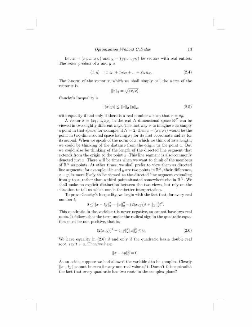
Let x = (x1, ..., xN ) and y = (y1, ..., yN ) be vectors with real entries.The inner product of x and y is
〈x, y〉 = x1y1 + x2y2 + ...+ xNyN . (2.4)
The 2-norm of the vector x, which we shall simply call the norm of thevector x is
‖x‖2 =√〈x, x〉.
Cauchy’s Inequality is
|〈x, y〉| ≤ ‖x‖2 ‖y‖2, (2.5)
with equality if and only if there is a real number a such that x = ay.A vector x = (x1, ..., xN ) in the real N -dimensional space RN can be
viewed in two slightly different ways. The first way is to imagine x as simplya point in that space; for example, if N = 2, then x = (x1, x2) would be thepoint in two-dimensional space having x1 for its first coordinate and x2 forits second. When we speak of the norm of x, which we think of as a length,we could be thinking of the distance from the origin to the point x. Butwe could also be thinking of the length of the directed line segment thatextends from the origin to the point x. This line segment is also commonlydenoted just x. There will be times when we want to think of the membersof RN as points. At other times, we shall prefer to view them as directedline segments; for example, if x and y are two points in RN , their difference,x − y, is more likely to be viewed as the directed line segment extendingfrom y to x, rather than a third point situated somewhere else in RN . Weshall make no explicit distinction between the two views, but rely on thesituation to tell us which one is the better interpretation.
To prove Cauchy’s Inequality, we begin with the fact that, for every realnumber t,
0 ≤ ‖x− ty‖22 = ‖x‖22 − (2〈x, y〉)t+ ‖y‖22t2.
This quadratic in the variable t is never negative, so cannot have two realroots. It follows that the term under the radical sign in the quadratic equa-tion must be non-positive, that is,
(2〈x, y〉)2 − 4‖y‖22‖x‖22 ≤ 0. (2.6)
We have equality in (2.6) if and only if the quadratic has a double realroot, say t = a. Then we have
‖x− ay‖22 = 0.
As an aside, suppose we had allowed the variable t to be complex. Clearly‖x− ty‖ cannot be zero for any non-real value of t. Doesn’t this contradictthe fact that every quadratic has two roots in the complex plane?

14 A First Course in Optimization
The Polya-Szego InequalityWe can interpret Cauchy’s Inequality as providing an upper bound for
the quantity ( N∑n=1
xnyn
)2.
The Polya-Szego Inequality provides a lower bound for the same quantity.Let 0 < m1 ≤ xn ≤M1 and 0 < m2 ≤ yn ≤M2, for all n. Then
N∑n=1
x2n
N∑n=1
y2n ≤M1M2 +m1m2√
4m1m2M1M2
( N∑n=1
xnyn
)2. (2.7)
2.8 Optimizing using Cauchy’s Inequality
We present three examples to illustrate the use of Cauchy’s Inequalityin optimization.
2.8.1 Example 4: A Constrained Optimization
Find the largest and smallest values of the function
f(x, y, z) = 2x+ 3y + 6z, (2.8)
among the points (x, y, z) with x2 + y2 + z2 = 1.From Cauchy’s Inequality we know that
49 = (22 + 32 + 62)(x2 + y2 + z2) ≥ (2x+ 3y + 6z)2,
so that f(x, y, z) lies in the interval [−7, 7]. We have equality in Cauchy’sInequality if and only if the vector (2, 3, 6) is parallel to the vector (x, y, z),that is
x
2=y
3=z
6.
It follows that x = t, y = 32 t, and z = 3t, with t2 = 4
49 . The smallest valueof f(x, y, z) is −7, when x = − 2
7 , and the largest value is +7, when x = 27 .
2.8.2 Example 5: A Basic Estimation Problem
The simplest problem in estimation theory is to estimate the value of aconstant c, given J data values zj = c + vj , j = 1, ..., J , where the vj arerandom variables representing additive noise or measurement error. Assume

Optimization Without Calculus 15
that the expected values of the vj are E(vj) = 0, the vj are uncorrelated,so E(vjvk) = 0 for j different from k, and the variances of the vj areE(v2j ) = σ2
j > 0. A linear estimate of c has the form
c =
J∑j=1
bjzj . (2.9)
The estimate c is unbiased if E(c) = c, which forces∑Jj=1 bj = 1. The best
linear unbiased estimator, the BLUE, is the one for which E((c − c)2) isminimized. This means that the bj must minimize
E( J∑j=1
J∑k=1
bjbkvjvk
)=
J∑j=1
b2jσ2j , (2.10)
subject to
J∑j=1
bj = 1. (2.11)
To solve this minimization problem, we turn to Cauchy’s Inequality.We can write
1 =
J∑j=1
bj =
J∑j=1
(bjσj)1
σj.
Cauchy’s Inequality then tells us that
1 ≤
√√√√ J∑j=1
b2jσ2j
√√√√ J∑j=1
1
σ2j
,
with equality if and only if there is a constant, say λ, such that
bjσj = λ1
σj,
for each j. So we have
bj = λ1
σ2j
,
for each j. Summing on both sides and using Equation (2.11), we find that
λ = 1/
J∑j=1
1
σ2j
.

16 A First Course in Optimization
The BLUE is therefore
c = λ
J∑j=1
zjσ2j
. (2.12)
When the variances σ2j are all the same, the BLUE is simply the arithmetic
mean of the data values zj .
2.8.3 Example 6: A Filtering Problem
One of the fundamental operations in signal processing is filtering thedata vector x = γs + n, to remove the noise component n, while leavingthe signal component s relatively unaltered [53]. This can be done eitherto estimate γ, the amount of the signal vector s present, or to detect ifthe signal is present at all, that is, to decide if γ = 0 or not. The noise istypically known only through its covariance matrix Q, which is the positive-definite, symmetric matrix having for its entries Qjk = E(njnk). The filterusually is linear and takes the form of an estimate of γ:
γ = bTx.
We want |bT s|2 large, and, on average, |bTn|2 small; that is, we wantE(|bTn|2) = bTE(nnT )b = bTQb small. The best choice is the vector bthat maximizes the gain of the filter, that is, the ratio
|bT s|2/bTQb.
We can solve this problem using the Cauchy Inequality.
Definition 2.2 Let S be a square matrix. A non-zero vector u is an eigen-vector of S if there is a scalar λ such that Su = λu. Then the scalar λ issaid to be an eigenvalue of S associated with the eigenvector u.
Definition 2.3 The transpose, B = AT , of an M by N matrix A is theN by M matrix having the entries Bn,m = Am,n.
Definition 2.4 A square matrix S is symmetric if ST = S.
A basic theorem in linear algebra is that, for any symmetric N by Nmatrix S, RN has an orthonormal basis consisting of mutually orthogonal,norm-one eigenvectors of S. We then define U to be the matrix whosecolumns are these orthonormal eigenvectors un and L the diagonal matrixwith the associated eigenvalues λn on the diagonal, we can easily see thatU is an orthogonal matrix, that is, UTU = I. We can then write
S = ULUT ; (2.13)

Optimization Without Calculus 17
this is the eigenvalue/eigenvector decomposition of S. The eigenvalues of asymmetric S are always real numbers.
Definition 2.5 A J by J symmetric matrix Q is non-negative definite if,for every x in RJ , we have xTQx ≥ 0. If xTQx > 0 whenever x is not thezero vector, then Q is said to be positive definite.
We leave it to the reader to show, in Exercise 2.13, that the eigenval-ues of a non-negative (positive) definite matrix are always non-negative(positive).
A covariance matrix Q is always non-negative definite, since
xTQx = E(|J∑j=1
xjnj |2). (2.14)
Therefore, its eigenvalues are non-negative; typically, they are actually pos-itive, as we shall assume now. We then let C = U
√LUT , which is called the
symmetric square root of Q since Q = C2 = CTC. The Cauchy Inequalitythen tells us that
|bT s|2 = |bTCC−1s|2 ≤ [bTCCT b][sT (C−1)TC−1s],
with equality if and only if the vectors CT b and C−1s are parallel. It followsthat
b = α(CCT )−1s = αQ−1s,
for any constant α. It is standard practice to select α so that bT s = 1,therefore α = 1/sTQ−1s and the optimal filter b is
b =1
sTQ−1sQ−1s.
2.9 An Inner Product for Square Matrices
The trace of a square matrix M , denoted trM , is the sum of the entriesdown the main diagonal. Given square matrices A and B with real entries,the trace of the product BTA defines an inner product, that is
〈A,B〉 = tr(BTA),
where the superscript T denotes the transpose of a matrix. This innerproduct can then be used to define a norm of A, called the Frobenius norm,by
‖A‖F =√〈A,A〉 =
√tr(ATA). (2.15)

18 A First Course in Optimization
From the eigenvector/eigenvalue decomposition, we know that, for everysymmetric matrix S, there is an orthogonal matrix U such that
S = UD(λ(S))UT ,
where λ(S) = (λ1, ..., λN ) is a vector whose entries are eigenvalues of thesymmetric matrix S, and D(λ(S)) is the diagonal matrix whose entries arethe entries of λ(S). Then we can easily see that
‖S‖F = ‖λ(S)‖2.
Denote by [λ(S)] the vector of eigenvalues of S, ordered in non-increasingorder. We have the following result.
Theorem 2.1 (Fan’s Theorem) Any real symmetric matrices S and Rsatisfy the inequality
tr(SR) ≤ 〈[λ(S)], [λ(R)]〉,
with equality if and only if there is an orthogonal matrix U such that
S = UD([λ(S)])UT ,
andR = UD([λ(R)])UT .
From linear algebra, we know that S and R can be simultaneously diag-onalized if and only if they commute; this is a stronger condition thansimultaneous diagonalization.
If S and R are diagonal matrices already, then Fan’s Theorem tells usthat
〈λ(S), λ(R)〉 ≤ 〈[λ(S)], [λ(R)]〉.Since any real vectors x and y are λ(S) and λ(R), for some symmetric Sand R, respectively, we have the followingHardy-Littlewood-Polya Inequality:
〈x, y〉 ≤ 〈[x], [y]〉.
Most of the optimization problems discussed in this chapter fall underthe heading of Geometric Programming, which we shall present in a moreformal way in a subsequent chapter.
2.10 Discrete Allocation Problems
Most of the optimization problems we consider in this book are con-tinuous problems, in the sense that the variables involved are free to take

Optimization Without Calculus 19
on values within a continuum. A large branch of optimization deals withdiscrete problems. Typically, these discrete problems can be solved, in prin-ciple, by an exhaustive checking of a large, but finite, number of possibili-ties; what is needed is a faster method. The optimal allocation problem isa good example of a discrete optimization problem.
We have n different jobs to assign to n different people. For i = 1, ..., nand j = 1, ..., n the quantity Cij is the cost of having person i do job j.The n by n matrix C with these entries is the cost matrix. An assignmentis a selection of n entries of C so that no two are in the same column or thesame row; that is, everybody gets one job. Our goal is to find an assignmentthat minimizes the total cost.
We know that there are n! ways to make assignments, so one solutionmethod would be to determine the cost of each of these assignments andselect the cheapest. But for large n this is impractical. We want an algo-rithm that will solve the problem with less calculation. The algorithm wepresent here, discovered in the 1930’s by two Hungarian mathematicians,is called, unimaginatively, the Hungarian Method.
To illustrate, suppose there are three people and three jobs, and thecost matrix is
C =
53 96 3747 87 4160 92 36
. (2.16)
The number 41 in the second row, third column indicates that it costs 41dollars to have the second person perform the third job.
The algorithm is as follows:
• Step 1: Subtract the minimum of each row from all the entries ofthat row. This is equivalent to saying that each person charges a min-imum amount just to be considered, which must be paid regardlessof the allocation made. All we can hope to do now is to reduce theremaining costs. Subtracting these fixed costs, which do not dependon the allocations, does not change the optimal solution.
The new matrix is then 16 59 06 46 024 56 0
. (2.17)
• Step 2: Subtract each column minimum from the entries of its col-umn. This is equivalent to saying that each job has a minimum cost,regardless of who performs it, perhaps for materials, say, or a permit.Subtracting those costs does not change the optimal solution. The
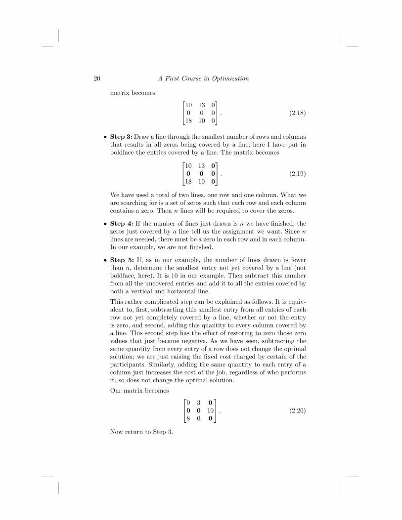
20 A First Course in Optimization
matrix becomes 10 13 00 0 018 10 0
. (2.18)
• Step 3: Draw a line through the smallest number of rows and columnsthat results in all zeros being covered by a line; here I have put inboldface the entries covered by a line. The matrix becomes10 13 0
0 0 018 10 0
. (2.19)
We have used a total of two lines, one row and one column. What weare searching for is a set of zeros such that each row and each columncontains a zero. Then n lines will be required to cover the zeros.
• Step 4: If the number of lines just drawn is n we have finished; thezeros just covered by a line tell us the assignment we want. Since nlines are needed, there must be a zero in each row and in each column.In our example, we are not finished.
• Step 5: If, as in our example, the number of lines drawn is fewerthan n, determine the smallest entry not yet covered by a line (notboldface, here). It is 10 in our example. Then subtract this numberfrom all the uncovered entries and add it to all the entries covered byboth a vertical and horizontal line.
This rather complicated step can be explained as follows. It is equiv-alent to, first, subtracting this smallest entry from all entries of eachrow not yet completely covered by a line, whether or not the entryis zero, and second, adding this quantity to every column covered bya line. This second step has the effect of restoring to zero those zerovalues that just became negative. As we have seen, subtracting thesame quantity from every entry of a row does not change the optimalsolution; we are just raising the fixed cost charged by certain of theparticipants. Similarly, adding the same quantity to each entry of acolumn just increases the cost of the job, regardless of who performsit, so does not change the optimal solution.
Our matrix becomes 0 3 00 0 108 0 0
. (2.20)
Now return to Step 3.

Optimization Without Calculus 21
In our example, when we return to Step 3 we find that we need threelines now and so we are finished. There are two optimal allocations: oneis to assign the first job to the first person, the second job to the secondperson, and the third job to the third person, for a total cost of 176 dollars;the other optimal allocation is to assign the second person to the first job,the third person to the second job, and the first person to the third job,again with a total cost of 176 dollars.
2.11 Exercises
Ex. 2.1 [176] Suppose that, in order to reduce automobile gasoline con-sumption, the government sets a fuel-efficiency target of T km/liter, andthen decrees that, if an auto maker produces a make of car with fuel effi-ciency of b < T , then it must also produce a make of car with fuel efficiencyrT , for some r > 1, such that the average of rT and b is T . Assume thatthe car maker sells the same number of each make of car. The question is:Is this a good plan? Why or why not? Be specific and quantitative in youranswer. Hint: The correct answer is No!.
Ex. 2.2 Let A be the arithmetic mean of a finite set of positive numbers,with x the smallest of these numbers, and y the largest. Show that
xy ≤ A(x+ y −A),
with equality if and only if x = y = A.
Ex. 2.3 Some texts call a function f(x) convex if
f(αx+ (1− α)y) ≤ αf(x) + (1− α)f(y)
for all x and y in the domain of the function and for all α in the interval[0, 1]. For this exercise, let us call this two-convex. Show that this definitionis equivalent to the one given in Definition 2.1. Hints: first, give the appro-priate definition of three-convex. Then show that three-convex is equivalentto two-convex; it will help to write
α1x1 + α2x2 = (1− α3)[α1
(1− α3)x1 +
α2
(1− α3)x2].
Finally, use induction on the number N .
Ex. 2.4 Minimize the function
f(x) = x2 +1
x2+ 4x+
4
x,

22 A First Course in Optimization
over positive x. Note that the minimum value of f(x, y) cannot be foundby a straight-forward application of the AGM Inequality to the four termstaken together. Try to find a way of rewriting f(x), perhaps using more thanfour terms, so that the AGM Inequality can be applied to all the terms.
Ex. 2.5 Find the maximum value of f(x, y) = x2y, if x and y are restrictedto positive real numbers for which 6x+ 5y = 45.
Ex. 2.6 Find the smallest value of
f(x) = 5x+16
x+ 21,
over positive x.
Ex. 2.7 Find the smallest value of the function
f(x, y) =√x2 + y2,
among those values of x and y satisfying 3x− y = 20.
Ex. 2.8 Find the maximum and minimum values of the function
f(x) =√
100 + x2 − x
over non-negative x.
Ex. 2.9 Multiply out the product
(x+ y + z)(1
x+
1
y+
1
z)
and deduce that the least value of this product, over non-negative x, y, andz, is 9. Use this to find the least value of the function
f(x, y, z) =1
x+
1
y+
1
z,
over non-negative x, y, and z having a constant sum c.
Ex. 2.10 The harmonic mean of positive numbers a1, ..., aN is
H = [(1
a1+ ...+
1
aN)/N ]−1.
Prove that the geometric mean G is not less than H.
Ex. 2.11 Prove that
(1
a1+ ...+
1
aN)(a1 + ...+ aN ) ≥ N2,
with equality if and only if a1 = ... = aN .

Optimization Without Calculus 23
Ex. 2.12 Show that the Equation (2.13), S = ULUT , can be written as
S = λ1u1(u1)T + λ2u
2(u2)T + ...+ λNuN (uN )T , (2.21)
and
S−1 =1
λ1u1(u1)T +
1
λ2u2(u2)T + ...+
1
λNuN (uN )T . (2.22)
Ex. 2.13 Show that a real symmetric matrix Q is non-negative (positive)definite if and only if all its eigenvalues are non-negative (positive).
Ex. 2.14 Let Q be positive-definite, with positive eigenvalues
λ1 ≥ ... ≥ λN > 0
and associated mutually orthogonal norm-one eigenvectors un. Show that
xTQx ≤ λ1,
for all vectors x with ‖x‖2 = 1, with equality if x = u1. Hints: use
1 = ‖x‖2 = xTx = xT Ix,
I = u1(u1)T + ...+ uN (uN )T ,
and Equation (2.21).
Ex. 2.15 Relate Example 4 to eigenvectors and eigenvalues.
Ex. 2.16 Young’s Inequality Suppose that p and q are positive numbersgreater than one such that 1
p + 1q = 1. If x and y are positive numbers, then
xy ≤ xp
p+yq
q,
with equality if and only if xp = yq. Hint: use the GAGM Inequality.
Ex. 2.17 ([167]) For given constants c and d, find the largest and smallestvalues of cx+ dy taken over all points (x, y) of the ellipse
x2
a2+y2
b2= 1.
Ex. 2.18 ([167]) Find the largest and smallest values of 2x + y on thecircle x2 + y2 = 1. Where do these values occur? What does this have to dowith eigenvectors and eigenvalues?

24 A First Course in Optimization
Ex. 2.19 When a real M by N matrix A is stored in the computer it isusually vectorized; that is, the matrix
A =
A11 A12 . . . A1N
A21 A22 . . . A2N
.
.
.AM1 AM2 . . . AMN
becomes
vec(A) = (A11, A21, ..., AM1, A12, A22, ..., AM2, ..., AMN )T .
Show that the dot product vec(A)·vec(B) = vec(B)Tvec(A) can be ob-tained by
vec(A)·vec(B) = trace (ABT ) = trace (BTA).
Ex. 2.20 Apply the Hungarian Method to solve the allocation problem withthe cost matrix
C =
90 75 75 8035 85 55 65125 95 90 10545 110 95 115
. (2.23)
You should find that the minimum cost is 275 dollars.

Chapter 3
Geometric Programming
3.1 Chapter Summary . . . . . . . . . . . . . . . . . . . . . . . . . . . . . . . . . . . . . . . . . . . . . . . 253.2 An Example of a GP Problem . . . . . . . . . . . . . . . . . . . . . . . . . . . . . . . . . . . 253.3 Posynomials and the GP Problem . . . . . . . . . . . . . . . . . . . . . . . . . . . . . . . 263.4 The Dual GP Problem . . . . . . . . . . . . . . . . . . . . . . . . . . . . . . . . . . . . . . . . . . . 283.5 Solving the GP Problem . . . . . . . . . . . . . . . . . . . . . . . . . . . . . . . . . . . . . . . . . 303.6 Solving the DGP Problem . . . . . . . . . . . . . . . . . . . . . . . . . . . . . . . . . . . . . . . 31
3.6.1 The MART . . . . . . . . . . . . . . . . . . . . . . . . . . . . . . . . . . . . . . . . . . . . . . 313.6.1.1 MART I . . . . . . . . . . . . . . . . . . . . . . . . . . . . . . . . . . . . 313.6.1.2 MART II . . . . . . . . . . . . . . . . . . . . . . . . . . . . . . . . . . . 32
3.6.2 Using the MART to Solve the DGP Problem . . . . . . . . . . . 323.7 Constrained Geometric Programming . . . . . . . . . . . . . . . . . . . . . . . . . . . 343.8 Exercises . . . . . . . . . . . . . . . . . . . . . . . . . . . . . . . . . . . . . . . . . . . . . . . . . . . . . . . . . 36
3.1 Chapter Summary
Geometric Programming (GP) involves the minimization of functionsof a special type, known as posynomials. The first systematic treatment ofgeometric programming appeared in the book [101], by Duffin, Petersonand Zener, the founders of geometric programming. As we shall see, theGeneralized Arithmetic-Geometric Mean Inequality plays an important rolein the theoretical treatment of geometric programming. In this chapter weintroduce the notions of duality and cross-entropy distance, and begin ourstudy of iterative algorithms. Some of this discussion of the GP problemfollows that in Peressini et al. [175].
3.2 An Example of a GP Problem
The following optimization problem was presented originally by Duffin,et al. [101] and discussed by Peressini et al. in [175]. It illustrates well the
25

26 A First Course in Optimization
type of problem considered in geometric programming. Suppose that 400cubic yards of gravel must be ferried across a river in an open box of lengtht1, width t2 and height t3. Each round-trip cost ten cents. The sides andthe bottom of the box cost 10 dollars per square yard to build, while theends of the box cost twenty dollars per square yard. The box will have nosalvage value after it has been used. Determine the dimensions of the boxthat minimize the total cost.
Although we know that the number of trips across the river must bea positive integer, we shall ignore that limitation in what follows, and use400/t1t2t3 as the number of trips. In this particular example, it will turnout that this quantity is a positive integer.
With t = (t1, t2, t3), the cost function is
g(t) =40
t1t2t3+ 20t1t3 + 10t1t2 + 40t2t3, (3.1)
which is to be minimized over ti > 0, for i = 1, 2, 3. The function g(t) is anexample of a posynomial.
3.3 Posynomials and the GP Problem
Functions g(t) of the form
g(t) =
n∑j=1
cj
( m∏i=1
taiji
), (3.2)
with t = (t1, ..., tm), the ti > 0, cj > 0 and aij real, are called posynomials.The geometric programming problem, denoted GP, is to minimize a givenposynomial over positive t. In order for the minimum to be greater thanzero, we need some of the aij to be negative.
We denote by uj(t) the function
uj(t) = cj
m∏i=1
taiji , (3.3)
so that
g(t) =
n∑j=1
uj(t). (3.4)
For any choice of δj > 0, j = 1, ..., n, with
n∑j=1
δj = 1,
Geometric Programming 27
we have
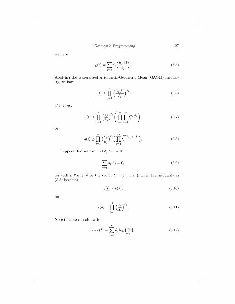
g(t) =
n∑j=1
δj
(uj(t)δj
). (3.5)
Applying the Generalized Arithmetic-Geometric Mean (GAGM) Inequal-ity, we have
g(t) ≥n∏j=1
(uj(t)δj
)δj. (3.6)
Therefore,
g(t) ≥n∏j=1
(cjδj
)δj( n∏j=1
m∏i=1
taijδji
), (3.7)
or
g(t) ≥n∏j=1
(cjδj
)δj( m∏i=1
t∑n
j=1 aijδji
), (3.8)
Suppose that we can find δj > 0 with
n∑j=1
aijδj = 0, (3.9)
for each i. We let δ be the vector δ = (δ1, ..., δn). Then the inequality in(3.8) becomes
g(t) ≥ v(δ), (3.10)
for
v(δ) =
n∏j=1
(cjδj
)δj. (3.11)
Note that we can also write
log v(δ) =
n∑j=1
δj log(cjδj
). (3.12)

28 A First Course in Optimization
3.4 The Dual GP Problem
The dual geometric programming problem, denoted DGP, is to maximizethe function v(δ), over all feasible δ = (δ1, ..., δn), that is, all positive δ forwhich
n∑j=1
δj = 1, (3.13)
and
n∑j=1
aijδj = 0, (3.14)
for each i = 1, ...,m.Denote by A the m+1 by n matrix with entries Aij = aij , and Am+1,j =
1, for j = 1, ..., n and i = 1, ...,m. Then we can write Equations (3.13) and(3.14) as
Aδ = u =
00···01
.
Clearly, we have
g(t) ≥ v(δ), (3.15)
for any positive t and feasible δ. Of course, there may be no feasible δ, inwhich case DGP is said to be inconsistent.
As we have seen, the inequality in (3.15) is based on the GAGM In-equality. We have equality in the GAGM Inequality if and only if the termsin the arithmetic mean are all equal. In this case, this says that there is aconstant λ such that
uj(t)
δj= λ, (3.16)
for each j = 1, ..., n. Using the fact that the δj sum to one, it follows that
λ =
n∑j=1
uj(t) = g(t), (3.17)

Geometric Programming 29
and
δj =uj(t)
g(t), (3.18)
for each j = 1, ..., n.As the theorem below asserts, if t∗ is positive and minimizes g(t), then
δ∗, the associated δ from Equation (3.18), is feasible and solves DGP. Sincewe have equality in the GAGM Inequality now, we have
g(t∗) = v(δ∗).
The main theorem in geometric programming is the following.
Theorem 3.1 If t∗ > 0 minimizes g(t), then DGP is consistent. In addi-tion, the choice
δ∗j =uj(t
∗)
g(t∗)(3.19)
is feasible and solves DGP. Finally,
g(t∗) = v(δ∗); (3.20)
that is, there is no duality gap.
Proof: We have
∂uj∂ti
(t∗) =aijuj(t
∗)
t∗i, (3.21)
so that
t∗i∂uj∂ti
(t∗) = aijuj(t∗), (3.22)
for each i = 1, ...,m. Since t∗ minimizes g(t), we have
0 =∂g
∂ti(t∗) =
n∑j=1
∂uj∂ti
(t∗), (3.23)
so that, from Equation (3.22), we have
0 =
n∑j=1
aijuj(t∗), (3.24)
for each i = 1, ...,m. It follows that δ∗ is feasible. Since
uj(t∗)/δ∗j = g(t∗) = λ,

30 A First Course in Optimization
for all j, we have equality in the GAGM Inequality, and we know
g(t∗) = v(δ∗). (3.25)
Therefore, δ∗ solves DGP. This completes the proof.
In Exercise 3.1 you are asked to show that the function
g(t1, t2) =2
t1t2+ t1t2 + t1
has no minimum over the region t1 > 0, and t2 > 0. As you will discover,the DGP is inconsistent in this case. We can still ask if there is a positivegreatest lower bound to the values that g can take on. Without too muchdifficulty, we can determine that if t1 ≥ 1 then g(t1, t2) ≥ 3, while if t2 ≤ 1then g(t1, t2) ≥ 4. Therefore, our hunt for the greatest lower bound isconcentrated in the region described by 0 < t1 < 1, and t2 > 1. Since thereis no minimum, we must consider values of t2 going to infinity, but suchthat t1t2 does not go to infinity and t1t2 does not go to zero; therefore,
t1 must go to zero. Suppose we let t2 = f(t1)t1
, for some function f(t) such
that f(0) > 0. Then, as t1 goes to zero, g(t1, t2) goes to 2f(0) + f(0). The
exercise asks you to determine how small this limiting quantity can be.
3.5 Solving the GP Problem
The theorem suggests how we might go about solving GP. First, we tryto find a feasible δ∗ that maximizes v(δ). This means we have to find apositive solution to the system of m + 1 linear equations in n unknowns,given by
n∑j=1
δj = 1, (3.26)
andn∑j=1
aijδj = 0, (3.27)
for i = 1, ...,m, such that v(δ) is maximized. As we shall see, the multiplica-tive algebraic reconstruction technique (MART) is an iterative procedurethat we can use to find such δ. If there is no such vector, then GP has nominimizer. Once the desired δ∗ has been found, we set
δ∗j =uj(t
∗)
v(δ∗), (3.28)

Geometric Programming 31
for each j = 1, ..., n, and then solve for the entries of t∗. This last step canbe simplified by taking logs; then we have a system of linear equations tosolve for the values log t∗i .
3.6 Solving the DGP Problem
The iterative multiplicative algebraic reconstruction technique MARTcan be used to maximize the function v(δ), subject to linear equality con-straints, provided that the matrix involved has nonnegative entries. Wecannot apply the MART yet, because the matrix A does not satisfy theseconditions.
3.6.1 The MART
The Kullback-Leibler, or KL distance [141] between positive numbers aand b is
KL(a, b) = a loga
b+ b− a. (3.29)
We also define KL(a, 0) = +∞ and KL(0, b) = b. Extending to non-negative vectors a = (a1, ..., aJ)T and b = (b1, ..., bJ)T , we have
KL(a, b) =
J∑j=1
KL(aj , bj) =
J∑j=1
(aj log
ajbj
+ bj − aj).
The MART is an iterative algorithm for finding a non-negative solution ofthe system Px = y, for an I by J matrix P with non-negative entries andvector y with positive entries. We also assume that
sj =
I∑i=1
Pij > 0,
for all j = 1, ..., J . When discussing the MART, we say that the systemPx = y is consistent when it has non-negative solutions. We consider twodifferent versions of the MART.
3.6.1.1 MART I
The iterative step of the first version of MART, which we shall callMART I, is the following: for k = 0, 1, ..., and i = k(mod I) + 1, let
xk+1j = xkj
( yi(Pxk)i
)Pij/mi
,

32 A First Course in Optimization
for j = 1, ..., J , where the parameter mi is defined to be
mi = max{Pij |j = 1, ..., J}.
The MART I algorithm converges, in the consistent case, to the non-negative solution for which the KL distance KL(x, x0) is minimized.
3.6.1.2 MART II
The iterative step of the second version of MART, which we shall callMART II, is the following: for k = 0, 1, ..., and i = k(mod I) + 1, let
xk+1j = xkj
( yi(Pxk)i
)Pij/sjni
,
for j = 1, ..., J , where the parameter ni is defined to be
ni = max{Pijs−1j |j = 1, ..., J}.
The MART II algorithm converges, in the consistent case, to the non-negative solution for which the KL distance
J∑j=1
sjKL(xj , x0j )
is minimized.
3.6.2 Using the MART to Solve the DGP Problem
The entries on the bottom row of A are all one, as is the bottom en-try of the column vector u, since these entries correspond to the equation∑nj=1 δj = 1. By adding suitably large positive multiples of this last equa-
tion to the other equations in the system, we obtain an equivalent system,Bδ = r, for which the new matrix B and the new vector r have only positiveentries. Now we can apply the MART I algorithm to the system Bδ = r,letting I = m + 1, J = n, P = B, sj =
∑m+1i=1 Bij , for j = 1, ..., n, δ = x,
x0 = c and y = r. In the consistent case, the MART I algorithm will findthe non-negative solution that minimizes KL(x, x0), so we select x0 = c.Then the MART I algorithm finds the non-negative δ∗ satisfying Bδ∗ = r,or, equivalently, Aδ∗ = u, for which the KL distance
KL(δ, c) =
n∑j=1
(δj log
δjcj
+ cj − δj)
is minimized. Since we know thatn∑j=1
δj = 1,

Geometric Programming 33
it follows that minimizing KL(δ, c) is equivalent to maximizing v(δ). Usingδ∗, we find the optimal t∗ solving the GP problem.
For example, the linear system of equations Aδ = u corresponding tothe posynomial in Equation (3.1) is
Aδ = u =
−1 1 1 0−1 0 1 1−1 1 0 11 1 1 1
δ1δ2δ3δ4
=
0001
.Adding two times the last row to the other rows, the system becomes
Bδ = r =
1 3 3 21 2 3 31 3 2 31 1 1 1
δ1δ2δ3δ4
=
2221
.The matrix B and the vector r are now positive. We are ready to applythe MART.
The MART iteration is as follows. With i = k(mod (m+ 1)) + 1, mi =max {Bij |j = 1, 2, ..., n} and k = 0, 1, ..., let
δk+1j = δkj
( ri(Bδk)i
)m−1i Bij
.
Using the MART, beginning with δ0 = c, we find that the optimal δ∗ isδ∗ = (.4, .2, .2, .2)T . Now we find v(δ∗), which, by Theorem 3.1, equalsg(t∗).
We have
v(δ∗) =( 40
0.4
)0.4( 20
0.2
)0.2( 10
0.2
)0.2( 40
0.2
)0.2,
so that, after a little arithmetic, we discover that v(δ∗) = g(t∗) = 100; thelowest cost is one hundred dollars.
Using Equation (3.19) for i = 1, ..., 4, we have
u1(t∗) =40
t∗1t∗2t∗3
= 100δ∗1 = 40,
u2(t∗) = 20t∗1t∗3 = 100δ∗2 = 20,
u3(t∗) = 10t∗1t∗2 = 100δ∗3 = 20,
andu4(t∗) = 40t∗2t
∗3 = 100δ∗4 = 20.
Again, a little arithmetic reveals that t∗1 = 2, t∗2 = 1, and t∗3 = 0.5. Here wewere able to solve the system of nonlinear equations fairly easily. Generally,however, we will need to take logarithms of both sides of each equation,and then solve the resulting system of linear equations for the unknownsx∗i = log t∗i .

34 A First Course in Optimization
3.7 Constrained Geometric Programming
Consider now the following variant of the problem of transporting thegravel across the river. Suppose that the bottom and the two sides willbe constructed for free from scrap metal, but only four square yards areavailable. The cost function to be minimized becomes
g0(t) =40
t1t2t3+ 40t2t3, (3.30)
and the constraint is
g1(t) =t1t3
2+t1t2
4≤ 1. (3.31)
With δ1 > 0, δ2 > 0, and δ1 + δ2 = 1, we write
g0(t) = δ140
δ1t1t2t3+ δ2
40t2t3δ2
. (3.32)
Since 0 ≤ g1(t) ≤ 1, we have
g0(t) ≥(δ1
40
δ1t1t2t3+ δ2
40t2t3δ2
)(g1(t)
)λ, (3.33)
for any positive λ. The GAGM Inequality then tells us that
g0(t) ≥
(( 40
δ1t1t2t3
)δ1(40t2t3δ2
)δ2)(g1(t)
)λ, (3.34)
so that
g0(t) ≥
((40
δ1
)δ1(40
δ2
)δ2)t−δ11 tδ2−δ12 tδ2−δ13
(g1(t)
)λ. (3.35)
From the GAGM Inequality, we also know that, for δ3 > 0, δ4 > 0 andλ = δ3 + δ4,(
g1(t))λ≥ (λ)λ
(( 1
2δ3
)δ3( 1
4δ4
)δ4)tδ3+δ41 tδ42 t
δ33 . (3.36)
Combining the inequalities in (3.35) and (3.36), we obtain
g0(t) ≥ v(δ)t−δ1+δ3+δ41 t−δ1+δ2+δ42 t−δ1+δ2+δ33 , (3.37)
with
v(δ) =(40
δ1
)δ1(40
δ2
)δ2( 1
2δ3
)δ3( 1
4δ4
)δ4(δ3 + δ4
)δ3+δ4, (3.38)

Geometric Programming 35
and δ = (δ1, δ2, δ3, δ4).If we can find a positive vector δ with
δ1 + δ2 = 1,
−δ1 + δ3 + δ4 = 0,
−δ1 + δ2 + δ4 = 0
−δ1 + δ2 + δ3 = 0, (3.39)
then
g0(t) ≥ v(δ). (3.40)
In this particular case, there is a unique positive δ satisfying the equations(3.39), namely
δ∗1 =2
3, δ∗2 =
1
3, δ∗3 =
1
3, and δ∗4 =
1
3, (3.41)
and
v(δ∗) = 60. (3.42)
Therefore, g0(t) is bounded below by 60. If there is t∗ such that
g0(t∗) = 60, (3.43)
then we must have
g1(t∗) = 1, (3.44)
and equality in the GAGM Inequality. Consequently,
3
2
40
t∗1t∗2t∗3
= 3(40t∗2t∗3) = 60, (3.45)
and
3
2t∗1t∗3 =
3
4t∗1t∗2 = K. (3.46)
Since g1(t∗) = 1, we must have K = 32 . We solve these equations by taking
logarithms, to obtain the solution
t∗1 = 2, t∗2 = 1, and t∗3 =1
2. (3.47)
The change of variables ti = exi converts the constrained GP probleminto a constrained convex programming problem. The theory of the con-strained GP problem can then be obtained as a consequence of the theoryfor the convex problem, which we shall consider in a later chapter.

36 A First Course in Optimization
3.8 Exercises
Ex. 3.1 Show that there is no solution to the problem of minimizing thefunction
g(t1, t2) =2
t1t2+ t1t2 + t1, (3.48)
over t1 > 0, t2 > 0. Can g(t1, t2) ever be smaller than 2√
2?
Ex. 3.2 Minimize the function
g(t1, t2) =1
t1t2+ t1t2 + t1 + t2, (3.49)
over t1 > 0, t2 > 0. This will require some iterative numerical method forsolving equations.
Ex. 3.3 Program the MART algorithm and use it to verify the assertionsmade previously concerning the solutions of the two numerical examples.

Chapter 4
Basic Analysis
4.1 Chapter Summary . . . . . . . . . . . . . . . . . . . . . . . . . . . . . . . . . . . . . . . . . . . . . . . 374.2 Minima and Infima . . . . . . . . . . . . . . . . . . . . . . . . . . . . . . . . . . . . . . . . . . . . . . . 374.3 Limits . . . . . . . . . . . . . . . . . . . . . . . . . . . . . . . . . . . . . . . . . . . . . . . . . . . . . . . . . . . . 384.4 Completeness . . . . . . . . . . . . . . . . . . . . . . . . . . . . . . . . . . . . . . . . . . . . . . . . . . . . . 394.5 Continuity . . . . . . . . . . . . . . . . . . . . . . . . . . . . . . . . . . . . . . . . . . . . . . . . . . . . . . . . 414.6 Limsup and Liminf . . . . . . . . . . . . . . . . . . . . . . . . . . . . . . . . . . . . . . . . . . . . . . . 424.7 Another View . . . . . . . . . . . . . . . . . . . . . . . . . . . . . . . . . . . . . . . . . . . . . . . . . . . . 434.8 Semi-Continuity . . . . . . . . . . . . . . . . . . . . . . . . . . . . . . . . . . . . . . . . . . . . . . . . . . 444.9 Exercises . . . . . . . . . . . . . . . . . . . . . . . . . . . . . . . . . . . . . . . . . . . . . . . . . . . . . . . . . 45
4.1 Chapter Summary
In this chapter we present a review of some of the basic notions fromanalysis.
4.2 Minima and Infima
When we say that we seek the minimum value of a function f(x) overx within some set C we imply that there is a point z in C such thatf(z) ≤ f(x) for all x in C. Of course, this need not be the case. Forexample, take the function f(x) = x defined on the real numbers and Cthe set of positive real numbers. In such cases, instead of looking for theminimum of f(x) over x in C, we may seek the infimum or greatest lowerbound of the values f(x), over x in C.
Definition 4.1 We say that a number α is the infimum of a subset S ofR, abbreviated α = inf (S), or the greatest lower bound of S, abbreviatedα = glb (S), if two conditions hold:
• 1. α ≤ s, for all s in S; and
37
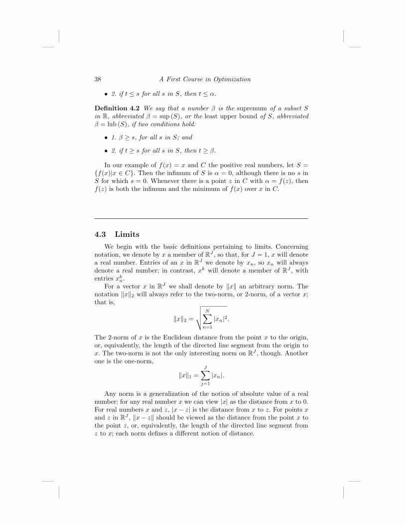
38 A First Course in Optimization
• 2. if t ≤ s for all s in S, then t ≤ α.
Definition 4.2 We say that a number β is the supremum of a subset Sin R, abbreviated β = sup (S), or the least upper bound of S, abbreviatedβ = lub (S), if two conditions hold:
• 1. β ≥ s, for all s in S; and
• 2. if t ≥ s for all s in S, then t ≥ β.
In our example of f(x) = x and C the positive real numbers, let S ={f(x)|x ∈ C}. Then the infimum of S is α = 0, although there is no s inS for which s = 0. Whenever there is a point z in C with α = f(z), thenf(z) is both the infimum and the minimum of f(x) over x in C.
4.3 Limits
We begin with the basic definitions pertaining to limits. Concerningnotation, we denote by x a member of RJ , so that, for J = 1, x will denotea real number. Entries of an x in RJ we denote by xn, so xn will alwaysdenote a real number; in contrast, xk will denote a member of RJ , withentries xkn.
For a vector x in RJ we shall denote by ‖x‖ an arbitrary norm. Thenotation ‖x‖2 will always refer to the two-norm, or 2-norm, of a vector x;that is,
‖x‖2 =
√√√√ N∑n=1
|xn|2.
The 2-norm of x is the Euclidean distance from the point x to the origin,or, equivalently, the length of the directed line segment from the origin tox. The two-norm is not the only interesting norm on RJ , though. Anotherone is the one-norm,
‖x‖1 =
J∑j=1
|xn|.
Any norm is a generalization of the notion of absolute value of a realnumber; for any real number x we can view |x| as the distance from x to 0.For real numbers x and z, |x− z| is the distance from x to z. For points xand z in RJ , ‖x− z‖ should be viewed as the distance from the point x tothe point z, or, equivalently, the length of the directed line segment fromz to x; each norm defines a different notion of distance.

Basic Analysis 39
In the definitions that follow we use an arbitrary norm on RJ . Thereason for this is that these definitions are independent of the particularnorm used. A sequence is bounded, Cauchy, or convergent with respect toone norm if and only if it is the same with respect to any norm. Similarly, afunction is continuous with respect to one norm if and only if it is continuouswith respect to any other norm.
Definition 4.3 A sequence {xn|n = 1, 2, ...}, xn ∈ RJ , is said to convergeto z ∈ RJ , or have limit z if, given any ε > 0, there is N = N(ε), usuallydepending on ε, such that
‖xn − z‖ ≤ ε,
whenever n ≥ N(ε).
Definition 4.4 A sequence {xn} in RJ is bounded if there is a constantB such that ‖xn‖ ≤ B, for all n.
It is convenient to extend the notion of limit of a sequence of realnumbers to include the infinities.
Definition 4.5 A sequence of real numbers {xn|n = 1, 2, ...} is said toconverge to +∞ if, given any b > 0, there is N = N(b), usually dependingon b, such that xn ≥ b, whenever n ≥ N(b). A sequence of real numbers{xn|n = 1, 2, ...} is said to converge to −∞ if the sequence {−xn} convergesto +∞.
Definition 4.6 Let f : RJ → RM . We say that z ∈ RM is the limit off(x), as x → a in RJ , if, for every sequence {xn} converging to a, withxn 6= a for all n, the sequence {f(xn)} in RM converges to z. We thenwrite
z = limx→a
f(x).
For M = 1, we allow z to be infinite.
4.4 Completeness
One version of the axiom of completeness for the set of real numbers Ris that every non-empty subset of R that is bounded above has a least up-per bound, or, equivalently, every non-empty subset of R that is boundedbelow has a greatest lower bound. The notion of completeness is usuallynot emphasized in beginning calculus courses and encountered for the first

40 A First Course in Optimization
time in a real analysis course. But without completeness, many of the fun-damental theorems in calculus would not hold. If we tried to do calculus byconsidering only rational numbers, the intermediate value theorem wouldnot hold, and it would be possible for a differentiable function to have apositive derivative without being increasing.
To further illustrate the importance of completeness, consider the proofof the following proposition.
Proposition 4.1 The sequence { 1n} converges to zero.
Suppose we attempt to prove this proposition simply by applying the def-inition of the limit of a sequence. Let ε > 0 be given. Select a positiveinteger N with N > 1
ε . Then, whenever n ≥ N , we have
| 1n− 0| = 1
n≤ 1
N< ε.
This would seem to complete the proof of the proposition. But it is incor-rect. The flaw in the argument is in the choice of N . We do not yet knowthat we can select N with N > 1
ε , since this is equivalent to 1N < ε. Until
we know that the proposition is true, we do not know that we can make 1N
as small as desired by the choice of N . The proof requires completeness.Let S be the set {1, 12 ,
13 ,
14 , ...}. This set is non-empty and bounded
below by any negative real number. Therefore, by completeness, S has agreatest lower bound; call it L. It is not difficult to prove that the decreasingsequence { 1n} must then converge to L, and the subsequence { 1
2n} mustalso converge to L. But since the limit of a product is the product of thelimits, whenever all the limits exist, we also know that the sequence { 1
2n}converges to L
2 . Therefore, L = L2 , and L = 0 must follow. Now the proof
is complete.The rational number line has “holes” in it that the irrational numbers
fill; in this sense, the completeness of the real numbers is sometimes char-acterized by saying that it has no holes in it. But the completeness of thereals actually tells us other things about the structure of the real numbers.We know, for example, that there are no rational numbers that are largerthan all the positive integers. But can there be irrational numbers that arelarger than all the positive integers? Completeness tells us that the answeris no.
Corollary 4.1 There is no real number larger than all the positive integers.
Proof: Suppose, to the contrary, that there is a real number b such thatb > n, for all positive integers n. Then 0 < 1
b <1n , for all positive integers n.
But this cannot happen, since, by the previous proposition, { 1n} convergesto zero.
Notice that, if we restrict ourselves to the world of rational numbers
Basic Analysis 41
when we define the concept of limit of a sequence, then we must also restrictthe ε to the rationals; suppose we call this the “rational limit”. When wedo this, we can show that the sequence { 1n} converges to zero. What wehave really shown with the proposition and corollary above is that, if asequence of rational numbers converges to a rational number, in the senseof the “rational limit”, then it converges to that rational number in theusual sense as well.
For the more general spaces RJ completeness is expressed, for example,by postulating that every Cauchy sequence is a convergent sequence.
Definition 4.7 A sequence {xn} of vectors in RJ is called a Cauchy se-quence if, for every ε > 0 there is a positive integer N = N(ε), usu-ally depending on ε, such that, for all m and n greater than N , we have‖xn − xm‖ < ε.
Every convergent sequence in RJ is bounded and is a Cauchy sequence.The Bolzano-Weierstrass Theorem tells us that every bounded sequence inRJ has a convergent subsequence; this is equivalent to the completeness ofthe metric space RJ .
Theorem 4.1 (The Bolzano-Weierstrass Theorem) Let {xn} be abounded sequence of vectors in RJ . Then {xn} has a convergent subse-quence.
4.5 Continuity
A basic notion in analysis is that of a continuous function. Although weshall be concerned primarily with functions whose values are real numbers,we can define continuity for functions whose values lie in RM .
Definition 4.8 We say the function f : RJ → RM is continuous at x = aif
f(a) = limx→a
f(x).
A basic theorem in real analysis is the following:
Theorem 4.2 Let f : RJ → R be continuous and let C be non-empty,closed, and bounded. Then there are a and b in C with f(a) ≤ f(x) andf(b) ≥ f(x), for all x in C.
We give some examples:

42 A First Course in Optimization
• 1. The function f(x) = x is continuous and the set C = [0, 1] is non-empty, closed and bounded. The minimum occurs at x = 0 and themaximum occurs at x = 1.
• 2. The set C = (0, 1] is not closed. The function f(x) = x has nominimum value on C, but does have a maximum value f(1) = 1.
• 3. The set C = (−∞, 0] is not bounded and f(x) = x has no minimumvalue on C. Note also that f(x) = x has no finite infimum with respectto C.
Definition 4.9 Let f : D ⊆ RJ → R. For any real α, the level set of fcorresponding to α is the set {x|f(x) ≤ α}.
Proposition 4.2 (Weierstrass) Suppose that f : D ⊆ RJ → R is con-tinuous, where D is non-empty and closed, and that every level set of f isbounded. Then f has a global minimizer.
Proof: This is a standard application of the Bolzano-Weierstrass Theorem.
4.6 Limsup and Liminf
Some of the functions we shall be interested in may be discontinuousat some points. For that reason, it is common in optimization to considersemi-continuity, which is weaker than continuity. While continuity involveslimits, semi-continuity involves superior and inferior limits.
We know that a real-valued function f(x) : RJ → R is continuous atx = a if, given any ε > 0, there is a δ > 0 such that ‖x − a‖ < δ impliesthat |f(x)− f(a)| < ε. We then write
f(a) = limx→a
f(x).
We can generalize this notion as follows.
Definition 4.10 We say that a finite real number β is the superior limitor lim sup of f(x), as x approaches a, written β = lim supx→a f(x) if,
• 1. for every ε > 0, there is δ > 0 such that, for every x satisfying‖x− a‖ < δ, we have f(x) < β + ε, and
• 2. for every ε > 0 and δ > 0 there is x with ‖x − a‖ < δ andf(x) > β − ε.
Basic Analysis 43
Definition 4.11 We say that a finite real number α is the inferior limitor lim inf of f(x), as x approaches a, written α = lim infx→a f(x) if,
• 1. for every ε > 0, there is δ > 0 such that, for every x satisfying‖x− a‖ < δ, we have f(x) > α− ε, and
• 2. for every ε > 0 and δ > 0 there is x with ‖x − a‖ < δ andf(x) < α+ ε.
We leave it as Exercise 4.4 for the reader to show that α =lim infx→a f(x) is the largest real number γ with the following property:for every ε > 0, there is δ > 0 such that, if ‖x− a‖ < δ, then f(x) > γ − ε.
Definition 4.12 We say that β = +∞ is the superior limit or lim sup off(x), as x approaches a, written +∞ = lim supx→a f(x) if, for every B > 0and δ > 0 there is x with ‖x− a‖ < δ and f(x) > B.
Definition 4.13 We say that α = −∞ is the inferior limit or lim inf off(x), as x approaches a, written −∞ = lim infx→a f(x) if, for every B > 0and δ > 0, there is x with ‖x− a‖ < δ and f(x) < −B.
It follows from the definitions that α ≤ f(a) ≤ β.For example, suppose that a = 0, f(x) = 0, for x 6= 0, and f(0) = 1.
Then β = 1 and α = 0. If a = 0, f(x) = −1/x for x < 0 and f(x) = 1/xfor x > 0, then α = −∞ and β = +∞.
It is not immediately obvious that β and α always exist. The nextsection provides another view of these notions, from which it becomes clearthat the existence of β and α is a consequence of the completeness of thespace R.
4.7 Another View
We can define the superior and inferior limits in terms of sequences. Weleave it to the reader to show that these definitions are equivalent to theones just given.
Let f : RJ → R and a be fixed in RJ . Let L be the set consisting ofall γ, possibly including the infinities, having the property that there is asequence {xn} in RJ converging to a such that {f(xn)} converges to γ. It isconvenient, now, to permit the sequence xn = a for all n, so that γ = f(a)is in L and L is never empty. Therefore, we always have
−∞ ≤ inf(L) ≤ f(a) ≤ sup(L) ≤ +∞.

44 A First Course in Optimization
For example, let f(x) = 1/x for x 6= 0, f(0) = 0, and a = 0. ThenL = {−∞, 0,+∞}, inf(L) = −∞, and sup(L) = +∞.
Definition 4.14 The (possibly infinite) number inf(L) is called the inferiorlimit or lim inf of f(x), as x → a in RJ . The (possibly infinite) numbersup(L) is called the superior limit or lim sup of f(x), as x→ a in RJ .
It follows from these definitions and our previous discussion that
lim infx→a
f(x) ≤ f(a) ≤ lim supx→a
f(x).
For example, let f(x) = x for x < 0 and f(x) = x+ 1 for x > 0. Thenwe have
lim supx→0
f(x) = 1,
andlim infx→0
f(x) = 0.
Proposition 4.3 The inferior limit and the superior limit are in the setL.
Proof: We leave the proof as Exercise 4.6.The function doesn’t have to be defined at a point in order for the
lim sup and lim inf to be defined there. If f : (0, δ) → R, for some δ > 0,we have the following definitions:
lim supt↓0
f(t) = limt↓0
(sup{f(x)|0 < x < t}
),
andlim inft↓0
f(t) = limt↓0
(inf{f(x)|0 < x < t}
).
4.8 Semi-Continuity
We know that α ≤ f(a) ≤ β. We can generalize the notion of continuityby replacing the limit with the inferior or superior limit. When M = 1, f(x)is continuous at x = a if and only if
lim infx→a
f(x) = lim supx→a
f(x) = f(a).
Definition 4.15 We say that f : RJ → R is lower semi-continuous (LSC)at x = a if
f(a) = α = lim infx→a
f(x).

Basic Analysis 45
Definition 4.16 We say that f : RJ → R is upper semi-continuous (USC)at x = a if
f(a) = β = lim supx→a
f(x).
Note that, if f(x) is LSC (USC) at x = a, then f(x) remains LSC (USC)when f(a) is replaced by any lower (higher) value. See Exercise 4.3 for anequivalent definition of lower semi-continuity.
The following theorem of Weierstrass extends Theorem 4.2 and showsthe importance of lower semi-continuity for minimization problems.
Theorem 4.3 Let f : RJ → R be LSC and let C be non-empty, closed,and bounded. Then there is a in C with f(a) ≤ f(x), for all x in C.
4.9 Exercises
Ex. 4.1 Let S and T be non-empty subsets of the real line, with s ≤ t forevery s in S and t in T . Prove that lub(S) ≤ glb(T ).
Ex. 4.2 Let f(x, y) : R2 → R, and, for each fixed y, let infx f(x, y) denotethe greatest lower bound of the set of numbers {f(x, y)|x ∈ R}. Show that
infx
(infyf(x, y)
)= inf
y
(infxf(x, y)
). (4.1)
Hint: note thatinfyf(x, y) ≤ f(x, y),
for all x and y.
Ex. 4.3 Prove that f : RJ → R is lower semi-continuous at x = a if andonly if, for every ε > 0, there is δ > 0 such that ‖x − a‖ < δ implies thatf(x) > f(a)− ε.
Ex. 4.4 Show that I = lim infx→a f(x) is the largest real number γ with thefollowing property: for every ε > 0, there is δ > 0 such that, if ‖x−a‖ < δ,then f(x) > γ − ε.
Ex. 4.5 Consider the function f(x) defined by f(x) = e−x, for x > 0 andby f(x) = −ex, for x < 0. Show that
−1 = lim infx→0
f(x)
and1 = lim sup
x→0f(x).

46 A First Course in Optimization
Ex. 4.6 For n = 1, 2, ..., let
An = {x| ‖x− a‖ ≤ 1
n},
and let αn and βn be defined by
αn = inf{f(x)|x ∈ An},
andβn = sup{f(x)|x ∈ An}.
• a) Show that the sequence {αn} is increasing, bounded above byf(a) and converges to some α, while the sequence {βn} is decreas-ing, bounded below by f(a) and converges to some β. Hint: use thefact that, if A ⊆ B, where A and B are sets of real numbers, theninf(A) ≥ inf(B).
• b) Show that α and β are in L. Hint: prove that there is a sequence{xn} with xn in An and f(xn) ≤ αn + 1
n .
• c) Show that, if {xm} is any sequence converging to a, then there isa subsequence, denoted {xmn}, such that xmn is in An, for each n.
• d) Show that, if {f(xm)} converges to γ, then
αn ≤ f(xmn) ≤ βn,
so thatα ≤ γ ≤ β.
• e) Show thatα = lim inf
x→af(x)
andβ = lim sup
x→af(x).

Chapter 5
Differentiation
5.1 Chapter Summary . . . . . . . . . . . . . . . . . . . . . . . . . . . . . . . . . . . . . . . . . . . . . . . 475.2 Directional Derivative . . . . . . . . . . . . . . . . . . . . . . . . . . . . . . . . . . . . . . . . . . . . 47
5.2.1 Definitions . . . . . . . . . . . . . . . . . . . . . . . . . . . . . . . . . . . . . . . . . . . . . . . 475.3 Partial Derivatives . . . . . . . . . . . . . . . . . . . . . . . . . . . . . . . . . . . . . . . . . . . . . . . 495.4 Some Examples . . . . . . . . . . . . . . . . . . . . . . . . . . . . . . . . . . . . . . . . . . . . . . . . . . 49
5.4.1 Example 1. . . . . . . . . . . . . . . . . . . . . . . . . . . . . . . . . . . . . . . . . . . . . . . . 495.4.2 Example 2. . . . . . . . . . . . . . . . . . . . . . . . . . . . . . . . . . . . . . . . . . . . . . . . 49
5.5 Gateaux Derivative . . . . . . . . . . . . . . . . . . . . . . . . . . . . . . . . . . . . . . . . . . . . . . 505.6 Frechet Derivative . . . . . . . . . . . . . . . . . . . . . . . . . . . . . . . . . . . . . . . . . . . . . . . . 51
5.6.1 The Definition . . . . . . . . . . . . . . . . . . . . . . . . . . . . . . . . . . . . . . . . . . . 515.6.2 Properties of the Frechet Derivative . . . . . . . . . . . . . . . . . . . . 51
5.7 The Chain Rule . . . . . . . . . . . . . . . . . . . . . . . . . . . . . . . . . . . . . . . . . . . . . . . . . . 515.8 A Useful Proposition . . . . . . . . . . . . . . . . . . . . . . . . . . . . . . . . . . . . . . . . . . . . . 525.9 Exercises . . . . . . . . . . . . . . . . . . . . . . . . . . . . . . . . . . . . . . . . . . . . . . . . . . . . . . . . . 53
5.1 Chapter Summary
The definition of the derivative of a function g : D ⊆ R→ R is a familiarone. In this chapter we examine various ways in which this definition canbe extended to functions f : D ⊆ RJ → R of several variables. Here D isthe domain of the function f and we assume that int(D), the interior ofthe set D, is not empty.
5.2 Directional Derivative
We begin with one- and two-sided directional derivatives.
47

48 A First Course in Optimization
5.2.1 Definitions
The function g(x) = |x| does not have a derivative at x = 0, but it hasone-sided directional derivatives there. The one-sided directional derivativeof g(x) at x = 0, in the direction of x = 1, is
g′+(0; 1) = limt↓0
1
t[g(0 + t)− g(0)] = 1, (5.1)
and in the direction of x = −1, it is
g′+(0;−1) = limt↓0
1
t[g(0− t)− g(0)] = 1. (5.2)
However, the two-sided derivative of g(x) = |x| does not exist at x = 0.We can extend the concept of one-sided directional derivatives to func-
tions of several variables.
Definition 5.1 Let f : D ⊆ RJ → R be a real-valued function of severalvariables, let a be in int(D), and let d be a unit vector in RJ . The one-sideddirectional derivative of f(x), at x = a, in the direction of d, is
f ′+(a; d) = limt↓0
1
t[f(a+ td)− f(a)]. (5.3)
Definition 5.2 The two-sided directional derivative of f(x) at x = a, inthe direction of d, is
f ′(a; d) = limt→0
1
t(f(a+ td)− f(a)). (5.4)
If the two-sided directional derivative exists then we have
f ′(a; d) = f ′+(a; d) = −f ′+(a;−d).
Given x = a and d, we define the function φ(t) = f(a+ td), for t such thata+ td is in D. The derivative of φ(t) at t = 0 is then
φ′(0) = limt→0
1
t[φ(t)− φ(0)] = f ′(a; d). (5.5)
In the definition of f ′(a; d) we restricted d to unit vectors because thedirectional derivative f ′(a; d) is intended to measure the rate of change off(x) as x moves away from x = a in the direction d. Later, in our discussionof convex functions, it will be convenient to view f ′(a; d) as a function ofd and to extend this function to the more general function of arbitrary zdefined by
f ′(a; z) = limt→0
1
t(f(a+ tz)− f(a)). (5.6)
It is easy to see that
f ′(a; z) = ‖z‖2f ′(a; z/‖z‖2).

Differentiation 49
5.3 Partial Derivatives
For j = 1, ..., J , denote by ej the vector whose entries are all zero,except for a one in the jth position.
Definition 5.3 If f ′(a; ej) exists, then it is ∂f∂xj
(a), the partial derivative
of f(x), at x = a, with respect to xj, the jth entry of the variable vector x.
Definition 5.4 If the partial derivative, at x = a, with respect to xj, existsfor each j, then the gradient of f(x), at x = a, is the vector ∇f(a) whoseentries are ∂f
∂xj(a).
5.4 Some Examples
We consider some examples of directional derivatives.
5.4.1 Example 1.
For (x, y) 6= (0, 0), let
f(x, y) =2xy
x2 + y2,
and define f(0, 0) = 1. Let d = (cos θ, sin θ). Then it is easy to show thatφ(t) = sin 2θ, for t 6= 0, and φ(0) = 1. If θ is such that sin 2θ = 1, then φ(t)is constant, and φ′(0) = 0. But, if sin 2θ 6= 1, then φ(t) is discontinuousat t = 0, so φ(t) is not differentiable at t = 0. Therefore, f(x, y) has atwo-sided directional derivative at (x, y) = (0, 0) only in certain directions.
5.4.2 Example 2.
[114] For (x, y) 6= (0, 0), let
f(x, y) =2xy2
x2 + y4,
and f(0, 0) = 0. Again, let d = (cos θ, sin θ). Then we have
φ′(0) =2 sin2 θ
cos θ,
50 A First Course in Optimization
for cos θ 6= 0. If cos θ = 0, then f(x) is the constant zero in that direction,so φ′(0) = 0. Therefore, the function f(x, y) has a two-sided directionalderivative at (x, y) = (0, 0), for every vector d. Note that the two partialderivatives are both zero at (x, y) = (0, 0), so ∇f(0, 0) = 0. Note also that,since f(y2, y) = 1 for all y 6= 0, the function f(x, y) is not continuous at(0, 0).
5.5 Gateaux Derivative
Just having a two-sided directional derivative for every d is not suffi-cient, in most cases; we need something stronger.
Definition 5.5 If f(x) has a two-sided directional derivative at x = a, forevery vector d, and, in addition,
f ′(a; d) = 〈∇f(a), d〉,
for each d, then f(x) is Gateaux-differentiable at x = a, and ∇f(a) is theGateaux derivative of f(x) at x = a, also denoted f ′(a).
Example 2 above showed that it is possible for f(x) to have a two-sideddirectional derivative at x = a, for every d, and yet fail to be Gateaux-differentiable.
From Cauchy’s Inequality, we know that
|f ′(a; d)| = |〈∇f(a), d〉| ≤ ||∇f(a)||2 ||d||2,
and that f ′(a; d) attains its most positive value when the direction d isa positive multiple of ∇f(a). This is the motivation for steepest descentoptimization.
For ordinary functions g : D ⊆ R → R, we know that differentiabilityimplies continuity. It is possible for f(x) to be Gateaux-differentiable atx = a and yet not be continuous at x = a; see Ortega and Rheinboldt[173]. This means that the notion of Gateaux-differentiability is too weak.In order to have a nice theory of multivariate differentiation, the notion ofderivative must be strengthened. The stronger notion we seek is Frechetdifferentiability.
Differentiation 51
5.6 Frechet Derivative
The notion of Frechet differentiability is the one appropriate for ourpurposes.
5.6.1 The Definition
Definition 5.6 We say that f(x) is Frechet-differentiable at x = a and∇f(a) is its Frechet derivative if
lim||h||→0
1
||h|||f(a+ h)− f(a)− 〈∇f(a), h〉| = 0.
Notice that the limit in the definition of the Frechet derivative involves thenorm of the incremental vector h, which is where the power of the Frechetderivative arises. Also, since the norm and the associated inner product canbe changed, so can the Frechet derivative; see Exercise 5.1 for an example.The corresponding limit in the definition of the Gateaux derivative involvesonly the scalar t, and therefore requires no norm and makes sense in anyvector space.
5.6.2 Properties of the Frechet Derivative
It can be shown that if f(x) is Frechet-differentiable at x = a, then f(x)is continuous at x = a. If f(x) is Gateaux-differentiable at each point in anopen set containing x = a, and ∇f(x) is continuous at x = a, then ∇f(a) isalso the Frechet derivative of f(x) at x = a. Since the continuity of ∇f(x)is equivalent to the continuity of each of the partial derivatives, we learnthat f(x) is Frechet-differentiable at x = a if it is Gateaux-differentiablein a neighborhood of x = a and the partial derivatives are continuous atx = a. If ∇f(x) is continuous in a neighborhood of x = a, the function f(x)is said to be continuously differentiable. Unless we write otherwise, when wesay that a function is differentiable, we shall mean Gateaux-differentiable,since this is usually sufficient for our purposes and the two types of differ-entiability typically coincide anyway.
5.7 The Chain Rule
For fixed a and d in RJ , the function φ(t) = f(a + td), defined for thereal variable t, is a composition of the function f : RJ → R itself and the

52 A First Course in Optimization
function g : R → RJ defined by g(t) = a + td; that is, φ(t) = f(g(t)).Writing
f(a+ td) = f(a1 + td1, a2 + td2, ..., aJ + tdJ),
and applying the Chain Rule, we find that
f ′(a; d) = φ′(0) =∂f
∂x1(a)d1 + ...+
∂f
∂xJ(a)dJ ;
that is,f ′(a; d) = φ′(0) = 〈∇f(a), d〉.
But we know that f ′(a; d) is not always equal to 〈∇f(a), d〉. This meansthat the Chain Rule is not universally true and must involve conditions onthe function f . Clearly, unless the function f is Gateaux-differentiable, thechain rule cannot hold. For an in-depth treatment of this matter, consultOrtega and Rheinboldt [173].
5.8 A Useful Proposition
The following proposition will be useful later in proving Gordan’s The-orem of the Alternative, Theorem 6.8.
Proposition 5.1 If the function f : RJ → R is differentiable and boundedbelow, that is, there is a constant α such that α ≤ f(x) for all x, then forevery ε > 0 there is a point xε with ‖∇f(xε)‖2 ≤ ε.
Proof: Fix ε > 0. The function f(x) + ε‖x‖2 has bounded level sets, so,by Proposition 4.2, it has a global minimizer, which we denote by xε. Weshow that d = ∇f(xε) has ‖d‖2 ≤ ε.
If not, then ‖d‖2 > ε. From the inequality
limt↓0
f(xε − td)− f(xε)
t= −〈∇f(xε), d〉 = −‖d‖22 < −ε‖d‖2
we would have, for small positive t,
−tε‖d‖2 > f(xε − td)− f(xε)
= (f(xε − td) + ε‖xε − td‖2)− (f(xε) + ε‖xε‖2)
+ε(‖xε‖2 − ‖xε − td‖2) ≥ −tε‖d‖2,
which is impossible.

Differentiation 53
5.9 Exercises
Ex. 5.1 Let Q be a real, positive-definite symmetric matrix. Define theQ-inner product on RJ to be
〈x, y〉Q = xTQy = 〈x,Qy〉,
and the Q-norm to be
||x||Q =√〈x, x〉Q.
Show that, if ∇f(a) is the Frechet derivative of f(x) at x = a, for the usualEuclidean norm, then Q−1∇f(a) is the Frechet derivative of f(x) at x = a,for the Q-norm. Hint: use the inequality√
λJ ||h||2 ≤ ||h||Q ≤√λ1||h||2,
where λ1 and λJ denote the greatest and smallest eigenvalues of Q, respec-tively.
Ex. 5.2 ([23], Ex. 10, p. 134) For (x, y) not equal to (0, 0), let
f(x, y) =xayb
xp + yq,
with f(0, 0) = 0. In each of the five cases below, determine if the functionis continuous, Gateaux, Frechet or continuously differentiable at (0, 0).
• 1) a = 2, b = 3, p = 2, and q = 4;
• 2) a = 1, b = 3, p = 2, and q = 4;
• 3) a = 2, b = 4, p = 4, and q = 8;
• 4) a = 1, b = 2, p = 2, and q = 2;
• 5) a = 1, b = 2, p = 2, and q = 4.


Chapter 6
Convex Sets
6.1 Chapter Summary . . . . . . . . . . . . . . . . . . . . . . . . . . . . . . . . . . . . . . . . . . . . . . . 556.2 The Geometry of Real Euclidean Space . . . . . . . . . . . . . . . . . . . . . . . . . 55
6.2.1 Inner Products . . . . . . . . . . . . . . . . . . . . . . . . . . . . . . . . . . . . . . . . . . . 566.2.2 Cauchy’s Inequality . . . . . . . . . . . . . . . . . . . . . . . . . . . . . . . . . . . . . . 576.2.3 Other Norms . . . . . . . . . . . . . . . . . . . . . . . . . . . . . . . . . . . . . . . . . . . . . 57
6.3 A Bit of Topology . . . . . . . . . . . . . . . . . . . . . . . . . . . . . . . . . . . . . . . . . . . . . . . . 576.4 Convex Sets in RJ . . . . . . . . . . . . . . . . . . . . . . . . . . . . . . . . . . . . . . . . . . . . . . . 59
6.4.1 Basic Definitions . . . . . . . . . . . . . . . . . . . . . . . . . . . . . . . . . . . . . . . . . 596.4.2 Orthogonal Projection onto Convex Sets . . . . . . . . . . . . . . . 63
6.5 Some Results on Projections . . . . . . . . . . . . . . . . . . . . . . . . . . . . . . . . . . . . . 666.6 Linear and Affine Operators on RJ . . . . . . . . . . . . . . . . . . . . . . . . . . . . . . 676.7 The Fundamental Theorems . . . . . . . . . . . . . . . . . . . . . . . . . . . . . . . . . . . . . 68
6.7.1 Basic Definitions . . . . . . . . . . . . . . . . . . . . . . . . . . . . . . . . . . . . . . . . . 686.7.2 The Separation Theorem . . . . . . . . . . . . . . . . . . . . . . . . . . . . . . . . 696.7.3 The Support Theorem . . . . . . . . . . . . . . . . . . . . . . . . . . . . . . . . . . . 69
6.8 Theorems of the Alternative . . . . . . . . . . . . . . . . . . . . . . . . . . . . . . . . . . . . . 716.9 Another Proof of Farkas’ Lemma . . . . . . . . . . . . . . . . . . . . . . . . . . . . . . . . 756.10 Gordan’s Theorem Revisited . . . . . . . . . . . . . . . . . . . . . . . . . . . . . . . . . . . . . 776.11 Exercises . . . . . . . . . . . . . . . . . . . . . . . . . . . . . . . . . . . . . . . . . . . . . . . . . . . . . . . . . 78
6.1 Chapter Summary
Convex sets and convex functions play important roles in optimization.In this chapter we survey the basic facts concerning the geometry of convexsets. We begin with the geometry of RJ .
6.2 The Geometry of Real Euclidean Space
We denote by RJ the real Euclidean space consisting of all J-dimensional column vectors x = (x1, ..., xJ)T with real entries xj ; here the
55

56 A First Course in Optimization
superscript T denotes the transpose of the 1 by J matrix (or, row vector)(x1, ..., xJ).
6.2.1 Inner Products
For x = (x1, ..., xJ)T and y = (y1, ..., yJ)T in RJ , the dot product x · yis defined to be
x · y =
J∑j=1
xjyj . (6.1)
Note that we can write
x · y = yTx = xT y, (6.2)
where juxtaposition indicates matrix multiplication. The 2-norm, or Eu-clidean norm, or Euclidean length, of x is
||x||2 =√x · x =
√xTx. (6.3)
The Euclidean distance between two vectors x and y in RJ is ||x− y||2.The space RJ , along with its dot product, is an example of a finite-
dimensional Hilbert space.
Definition 6.1 Let V be a real vector space. The scalar-valued function〈u, v〉 is called an inner product on V if the following four properties hold,for all u, w, and v in V , and all real c:
〈u+ w, v〉 = 〈u, v〉+ 〈w, v〉; (6.4)
〈cu, v〉 = c〈u, v〉; (6.5)
〈v, u〉 = 〈u, v〉; (6.6)
and
〈u, u〉 ≥ 0, (6.7)
with equality in Inequality (6.7) if and only if u = 0.
The dot product of vectors is an example of an inner product. The prop-erties of an inner product are precisely the ones needed to prove Cauchy’sInequality, which then holds for any inner product. We shall favor the dotproduct notation u · v for the inner product of vectors, although we shalloccasionally use the matrix multiplication form, vTu or the inner productnotation 〈u, v〉.

Convex Sets 57
6.2.2 Cauchy’s Inequality
Cauchy’s Inequality, also called the Cauchy-Schwarz Inequality, tells usthat
|〈x, y〉| ≤ ||x||2||y||2, (6.8)
with equality if and only if y = αx, for some scalar α. The Cauchy-SchwarzInequality holds for any inner product. We say that the vectors x and yare mutually orthogonal if 〈x, y〉 = 0.
A simple application of Cauchy’s inequality gives us
||x+ y||2 ≤ ||x||2 + ||y||2, (6.9)
with equality if and only if one of the vectors is a non-negative multiple ofthe other one; this is called the Triangle Inequality.
The Parallelogram Law is an easy consequence of the definition of the2-norm:
||x+ y||22 + ||x− y||22 = 2||x||22 + 2||y||22. (6.10)
It is important to remember that Cauchy’s Inequality and the Parallelo-gram Law hold only for the 2-norm. One consequence of the ParallelogramLaw that we shall need later is the following: if x 6= y and ‖x‖2 = ‖y‖2 = d,then ‖ 12 (x+ y)‖2 < d (Draw a picture!).
6.2.3 Other Norms
The two-norm is not the only norm we study on the space RJ . We willalso be interested in the one-norm (see Exercise 6.4). The purely topologicalresults we discuss in the next section are independent of the choice of normon RJ , and we shall remind the reader of this by using the notation ‖x‖ todenote an arbitrary norm. Theorems concerning orthogonal projection holdonly for the two-norm, which we shall denote by ‖x‖2. In fact, whenever weuse the word “orthogonal” , we shall imply that we are speaking about thetwo-norm. There have been attempts to define orthogonality in the absenceof an inner product, and so for other norms, but the theory here is not assuccessful.
6.3 A Bit of Topology
Having a norm allows us to define the distance between two points xand y in RJ as ||x − y||. Being able to talk about how close points are

58 A First Course in Optimization
to each other enables us to define continuity of functions on RJ and toconsider topological notions of closed set, open set, interior of a set andboundary of a set. None of these notions depend on the particular normwe are using.
Definition 6.2 A subset B of RJ is closed if, whenever xk is in B foreach non-negative integer k and ||x − xk|| → 0, as k → +∞, then x is inB.
For example, B = [0, 1] is closed as a subset of R, but B = (0, 1) is not.
Definition 6.3 We say that d ≥ 0 is the distance from the point x to theset B if, for every ε > 0, there is bε in B, with ||x− bε|| < d+ ε, and no bin B with ||x− b|| < d.
The Euclidean distance from the point 0 in R to the set (0, 1) is zero, whileits distance to the set (1, 2) is one. It follows easily from the definitionsthat, if B is closed and d = 0, then x is in B.
Definition 6.4 The closure of a set B is the set of all points x whosedistance from B is zero.
The closure of the interval B = (0, 1) is [0, 1].
Definition 6.5 A subset U of RJ is open if its complement, the set of allpoints not in U , is closed.
Definition 6.6 Let C be a subset of RJ . A point x in C is said to bean interior point of set C if there is ε > 0 such that every point z with||x− z|| < ε is in C. The interior of the set C, written int(C), is the set ofall interior points of C. It is also the largest open set contained within C.
For example, the open interval (0, 1) is the interior of the intervals (0, 1]and [0, 1]. A set C is open if and only if C = int(C).
Definition 6.7 A point x in RJ is said to be a boundary point of set Cif, for every ε > 0, there are points yε in C and zε not in C, both dependingon the choice of ε, with ||x − yε|| < ε and ||x − zε|| < ε. The boundary ofC is the set of all boundary points of C. It is also the intersection of theclosure of C with the closure of its complement.
For example, the points x = 0 and x = 1 are boundary points of the set(0, 1].
Definition 6.8 For k = 0, 1, 2, ..., let xk be a vector in RJ . The sequenceof vectors {xk} is said to converge to the vector z if, given any ε > 0, thereis positive integer n, usually depending on ε, such that, for every k > n,we have ||z − xk|| ≤ ε. Then we say that z is the limit of the sequence.

Convex Sets 59
For example, the sequence {xk = 1k+1} in R converges to z = 0. The
sequence {(−1)k} alternates between 1 and −1, so does not converge. How-ever, the subsequence associated with odd k converges to z = −1, while thesubsequence associated with even k converges to z = 1. The values z = −1and z = 1 are called subsequential limit points, or, sometimes, cluster pointsof the sequence.
Definition 6.9 A sequence {xk} of vectors in RJ is said to be bounded ifthere is a constant b > 0, such that ||xk|| ≤ b, for all k.
A fundamental result in analysis is the following.
Proposition 6.1 Every convergent sequence of vectors in RJ is bounded.Every bounded sequence of vectors in RJ has at least one convergent sub-sequence, therefore, has at least one cluster point.
6.4 Convex Sets in RJ
In preparation for our discussion of linear and nonlinear programming,we consider some of the basic concepts from the geometry of convex sets.
6.4.1 Basic Definitions
We begin with the basic definitions.
Definition 6.10 A vector z is said to be a convex combination of thevectors x and y if there is α in the interval [0, 1] such that z = (1−α)x+αy.More generally, a vector z is a convex combination of the vectors xn, n =1, ..., N , if there are numbers αn ≥ 0 with
α1 + ...+ αN = 1
andz = α1x
1 + ...+ αNxN .
Definition 6.11 A nonempty set C in RJ is said to be convex if, for anydistinct points x and y in C, and for any real number α in the interval(0, 1), the point (1 − α)x + αy is also in C; that is, C is closed to convexcombinations of any two members of C.

60 A First Course in Optimization
In Exercise 6.1 you are asked to show that if C is convex then the convexcombination of any number of members of C is again in C. We say thenthat C is closed to convex combinations.
For example, the two-norm unit ball B in RJ , consisting of all x with||x||2 ≤ 1, is convex, while the surface of the ball, the set of all x with||x||2 = 1, is not convex. More generally, the unit ball of RJ in any normis a convex set, as a consequence of the triangle inequality for norms.
Definition 6.12 The convex hull of a set S, denoted conv(S), is the small-est convex set containing S, by which we mean that if K is any convex setcontaining S, then K must also contain conv(S).
One weakness of this definition is that it does not tell us explicitly what themembers of conv(S) look like, nor precisely how the individual membersof conv(S) are related to the members of S itself. In fact, it is not obviousthat a smallest such set exists at all. The following proposition remediesthis; the reader is asked to supply a proof in Exercise 6.2 later.
Proposition 6.2 The convex hull of a set S is the set C of all convexcombinations of members of S.
Definition 6.13 A subset S of RJ is a subspace if, for every x and y inS and scalars α and β, the linear combination αx+ βy is again in S.
A subspace is necessarily a convex set.
Definition 6.14 The orthogonal complement of a subspace S of RJ , en-dowed with the two-norm, is the set
S⊥ = {u|〈u, s〉 = u · s = uT s = 0, for every s ∈ S}, (6.11)
the set of all vectors u in RJ that are orthogonal to every member of S.
For example, in R3, the x, y-plane is a subspace and has for its orthog-onal complement the z-axis.
Definition 6.15 A subset M of RJ is a linear manifold if there is a sub-space S and a vector b such that
M = S + b = {x|x = s+ b, for some s inS}.
Any linear manifold is convex.
Definition 6.16 For a fixed column vector a with Euclidean length oneand a fixed scalar γ the hyperplane determined by a and γ is the set
H(a, γ) = {z|〈a, z〉 = γ}.

Convex Sets 61
The hyperplanes H(a, γ) are linear manifolds, and the hyperplanesH(a, 0) are subspaces. Hyperplanes in RJ are naturally associated with lin-ear equations in J variables; with a = (a1, ..., aJ)T , the hyperplane H(a, γ)is the set of all z = (z1, ..., zJ)T for which
a1z1 + a2z2 + ...+ aJzJ = γ.
Earlier, we mentioned that there are two related, but distinct, ways toview members of the set RJ . The first is to see x in RJ as a point in J-dimensional space, so that, for example, if J = 2, then a member x of R2
can be thought of as a point in a plane, the plane of the blackboard, say.The second way is to think of x is as the directed line segment from theorigin to the point also denoted x. We purposely avoided making a choicebetween one interpretation and the other because there are cases in whichwe want to employ both interpretations; the definition of the hyperplaneH(a, γ) provides just such a case. We want to think of the members of thehyperplane as points in RJ that lie within the set H(a, γ), but we wantto think of a as a directed line segment perpendicular, or normal, to thehyperplane. When x, viewed as a point, is in H(a, γ), the directed linesegment from the origin to x will not lie in the hyperplane, unless γ = 0.
Lemma 6.1 The distance from the hyperplane H(a, γ) to the hyperplaneH(a, γ + 1) is one.
The proof is left as Exercise 6.8.
Definition 6.17 For each vector a and each scalar γ, the sets
H+(a, γ) = {z|〈a, z〉 ≥ γ}
H−(a, γ) = {z|〈a, z〉 ≤ γ}
are half-spaces.
Half-spaces in RJ are naturally associated with linear inequalities in Jvariables; with a = (a1, ..., aJ)T , the half-space H+(a, γ) is the set of allz = (z1, ..., zJ)T for which
a1z1 + a2z2 + ...+ aJzJ ≥ γ.
Perhaps the most important convex sets in optimization are the poly-hedrons:
Definition 6.18 A subset P of RJ is a polyhedron if P is the intersectionof a finite number of half-spaces.

62 A First Course in Optimization
A polyhedron is the set of all vectors that satisfy a finite number oflinear inequalities: the set P in R2 consisting of all vectors (x1, x2) withx1 ≥ 0, x2 ≥ 0 is an unbounded polyhedron, while the set B in R2 consistingof all vectors (x1, x2) with x1 ≥ 0, x2 ≥ 0 and x1 + x2 ≤ 1 is a boundedpolyhedron. The set B is also the convex hull of a finite set of points, namelythe three points (0, 0), (1, 0) and (0, 1), and therefore is also a polytope.
Definition 6.19 Given a subset C of RJ , the affine hull of C, denotedaff(C), is the smallest linear manifold containing C.
For example, let C be the line segment connecting the two points (0, 1)and (1, 2) in R2. The affine hull of C is the straight line whose equation isy = x+ 1.
Definition 6.20 The dimension of a subset of RJ is the dimension of itsaffine hull, which is the dimension of the subspace of which it is a translate.
The set C above has dimension one. A set containing only one point is itsown affine hull, since it is a translate of the subspace {0}.
In R2, the line segment connecting the points (0, 1) and (1, 2) has nointerior; it is a one-dimensional subset of a two-dimensional space and cancontain no two-dimensional ball. But, the part of this set without its twoend points is a sort of interior, called the relative interior.
Definition 6.21 The relative interior of a subset C of RJ , denoted ri(C),is the interior of C, as defined by considering C as a subset of its affinehull.
Since a set consisting of a single point is its own affine hull, it is its ownrelative interior.
Definition 6.22 A point x in a convex set C is said to be an extremepoint of C if the set obtained by removing x from C remains convex.
Said another way, x ∈ C is an extreme point of C if x is not a convexcombination of two other points in C; that is, x cannot be written as
x = (1− α)y + αz, (6.12)
for y and z in C, y, z 6= x and α ∈ (0, 1). For example, the point x = 1 isan extreme point of the convex set C = [0, 1]. Every point on the boundaryof a sphere in RJ is an extreme point of the sphere. The set of all extremepoints of a convex set is denoted Ext(C).
Definition 6.23 A non-zero vector d is said to be a direction of unbound-edness of a convex set C if, for all x in C and all γ ≥ 0, the vector x+ γdis in C.

Convex Sets 63
For example, if C is the non-negative orthant in RJ , then any non-negativevector d is a direction of unboundedness.
Definition 6.24 A vector a is normal to a convex set C at the point s inC if
〈a, c− s〉 ≤ 0, (6.13)
for all c in C.
Definition 6.25 Let C be convex and s in C. The normal cone to C at s,denoted NC(s), is the set of all vectors a that are normal to C at s.
Normality and the normal cone are notions that make sense only in aspace with an inner product, so are implicitly connected to the two-norm.
6.4.2 Orthogonal Projection onto Convex Sets
The following proposition is fundamental in the study of convexity andcan be found in most books on the subject; see, for example, the text byGoebel and Reich [118].
Proposition 6.3 Given any nonempty closed convex set C and an arbi-trary vector x in RJ , there is a unique member PCx of C closest, in thesense of the two-norm, to x. The vector PCx is called the orthogonal (ormetric) projection of x onto C and the operator PC the orthogonal projec-tion onto C.
Proof: If x is in C, then PCx = x, so assume that x is not in C. Thend > 0, where d is the distance from x to C. For each positive integer n,select cn in C with ||x− cn||2 < d+ 1
n . Then, since for all n we have
‖cn‖2 = ‖cn − x+ x‖2 ≤ ‖cn − x‖2 + ‖x‖2 ≤ d+1
n+ ‖x‖2 < d+ 1 + ‖x‖2,
the sequence {cn} is bounded; let c∗ be any cluster point. It follows easilythat ||x − c∗||2 = d and that c∗ is in C. If there is any other member cof C with ||x − c||2 = d, then, by the Parallelogram Law, we would have||x− (c∗ + c)/2||2 < d, which is a contradiction. Therefore, c∗ is PCx.
The proof just given relies on the Bolzano-Weierstrass Theorem 4.1.There is another proof, which avoids this theorem and so is valid for infinite-dimensional Hilbert space. The idea is to use the Parallelogram Law to showthat the sequence {cn} is Cauchy and then to use completeness to get c∗.We leave the details to the reader.
Here are some examples of orthogonal projection. If C = U , the unitball, then PCx = x/||x||2, for all x such that ||x||2 > 1, and PCx = x

64 A First Course in Optimization
otherwise. If C is RJ+, the nonnegative cone of RJ , consisting of all vectorsx with xj ≥ 0, for each j, then PCx = x+, the vector whose entries aremax (xj , 0). For any closed, convex set C, the distance from x to C is||x− PCx||2.
If a nonempty closed set S is not convex, then the orthogonal projectionof a vector x onto S need not be well defined; there may be more than onevector in S closest to x. In fact, it is known that a closed set S is convex ifand only if, for every x not in S, there is a unique point in S closest to x;this is Motzkin’s Theorem (see [24], p. 447). Note that there may well besome x for which there is a unique closest point in S, but if S is closed, butnot convex, then there must be at least one point without a unique closestpoint in S.
The main reason for not speaking about orthogonal projection in thecontext of other norms is that there need not be a unique closest point inC to x; remember that the Parallelogram Law need not hold. For example,consider the closed convex set C in R2 consisting of all vectors (a, b)T witha ≥ 0, b ≥ 0, and a + b = 1. Let x = (1, 1)T . Then each point in C is adistance one from x, in the sense of the one-norm.
Lemma 6.2 For H = H(a, γ), z = PHx is the vector
z = PHx = x+ (γ − 〈a, x〉)a. (6.14)
We shall use this fact in our discussion of the ART algorithm.For an arbitrary nonempty closed convex set C in RJ , the orthogonal
projection T = PC is a nonlinear operator, unless, of course, C is a sub-space. We may not be able to describe PCx explicitly, but we do know auseful property of PCx.
Proposition 6.4 For a given x, a vector z in C is PCx if and only if
〈c− z, z − x〉 ≥ 0, (6.15)
for all c in the set C.
Proof: Let c be arbitrary in C and α in (0, 1). Then
||x− PCx||22 ≤ ||x− (1− α)PCx− αc||22 = ||x− PCx+ α(PCx− c)||22
= ||x− PCx||22 − 2α〈x− PCx, c− PCx〉+ α2||PCx− c||22. (6.16)
Therefore,
−2α〈x− PCx, c− PCx〉+ α2||PCx− c||22 ≥ 0, (6.17)
so that
2〈x− PCx, c− PCx〉 ≤ α||PCx− c||22. (6.18)

Convex Sets 65
Taking the limit, as α→ 0, we conclude that
〈c− PCx, PCx− x〉 ≥ 0. (6.19)
If z is a member of C that also has the property
〈c− z, z − x〉 ≥ 0, (6.20)
for all c in C, then we have both
〈z − PCx, PCx− x〉 ≥ 0, (6.21)
and
〈z − PCx, x− z〉 ≥ 0. (6.22)
Adding on both sides of these two inequalities lead to
〈z − PCx, PCx− z〉 ≥ 0. (6.23)
But,
〈z − PCx, PCx− z〉 = −||z − PCx||22, (6.24)
so it must be the case that z = PCx. This completes the proof.
Corollary 6.1 For any x and y in RJ we have
〈PCx− PCy, x− y〉 ≥ ‖PCx− PCy‖22. (6.25)
Proof: Use Inequality (6.4) to get
〈PCy − PCx, PCx− x〉 ≥ 0, (6.26)
and
〈PCx− PCy, PCy − y〉 ≥ 0. (6.27)
Add the two inequalities to obtain
〈PCx− PCy, x− y〉 ≥ ||PCx− PCy||22. (6.28)
66 A First Course in Optimization
6.5 Some Results on Projections
The characterization of the orthogonal projection operator PC given byProposition 6.4 has a number of important consequences.
Corollary 6.2 Let S be any subspace of RJ . Then, for any x in RJ and sin S, we have
〈PSx− x, s〉 = 0. (6.29)
Proof: Since S is a subspace, s+ PSx is again in S, for all s, as is γs, forevery scalar γ.
This corollary enables us to prove the Decomposition Theorem.
Theorem 6.1 Let S be any subspace of RJ and x any member of RJ . Thenthere are unique vectors s in S and u in S⊥ such that x = s+u. The vectors is PSx and the vector u is PS⊥x.
Proof: For the given x we take s = PSx and u = x − PSx. Corollary 6.2assures us that u is in S⊥. Now we need to show that this decomposition isunique. To that end, suppose that we can write x = s1 + u1, with s1 in Sand u1 in S⊥. Then Proposition 6.4 tells us that, since s1−x is orthogonalto every member of S, s1 must be PSx.
This theorem is often presented in a slightly different manner.
Theorem 6.2 Let A be a real I by J matrix. Then every vector b in RIcan be written uniquely as b = Ax+ w, where ATw = 0.
To derive Theorem 6.2 from Theorem 6.1, we simply let S = {Ax|x ∈ RJ}.Then S⊥ is the set of all w such that ATw = 0. It follows that w is themember of the null space of AT closest to b.
Here are additional consequences of Proposition 6.4.
Corollary 6.3 Let S be any subspace of RJ , d a fixed vector, and V thelinear manifold V = S+ d = {v = s+ d|s ∈ S}, obtained by translating themembers of S by the vector d. Then, for every x in RJ and every v in V ,we have
〈PV x− x, v − PV x〉 = 0. (6.30)
Proof: Since v and PV x are in V , they have the form v = s + d, andPV x = s+ d, for some s and s in S. Then v − PV x = s− s.

Convex Sets 67
Corollary 6.4 Let H be the hyperplane H(a, γ). Then, for every x, andevery h in H, we have
〈PHx− x, h− PHx〉 = 0. (6.31)
Corollary 6.5 Let S be a subspace of RJ . Then (S⊥)⊥ = S.
Proof: Every x in RJ has the form x = s + u, with s in S and u in S⊥.Suppose x is in (S⊥)⊥. Then u = 0.
6.6 Linear and Affine Operators on RJ
If A is a J by J real matrix, then we can define an operator T bysetting Tx = Ax, for each x in RJ ; here Ax denotes the multiplication ofthe matrix A and the column vector x.
Definition 6.26 An operator T is said to be a linear operator if
T (αx+ βy) = αTx+ βTy, (6.32)
for each pair of vectors x and y and each pair of scalars α and β.
Any operator T that comes from matrix multiplication, that is, for whichTx = Ax, is linear.
Lemma 6.3 For H = H(a, γ), H0 = H(a, 0), and any x and y in RJ , wehave
PH(x+ y) = PHx+ PHy − PH0, (6.33)
so that
PH0(x+ y) = PH0
x+ PH0y, (6.34)
that is, the operator PH0is an additive operator. In addition,
PH0(αx) = αPH0
x, (6.35)
so that PH0 is a linear operator.
Definition 6.27 If A is a J by J real matrix and d is a fixed nonzero vectorin RJ , the operator defined by Tx = Ax+ d is an affine linear operator.
68 A First Course in Optimization
Lemma 6.4 For any hyperplane H = H(a, γ) and H0 = H(a, 0),
PHx = PH0x+ PH0, (6.36)
so PH is an affine linear operator.
Lemma 6.5 For i = 1, ..., I let Hi be the hyperplane Hi = H(ai, γi),Hi0 = H(ai, 0), and Pi and Pi0 the orthogonal projections onto Hi and Hi0,respectively. Let T be the operator T = PIPI−1 · · ·P2P1. Then Tx = Bx+d,for some square matrix B and vector d; that is, T is an affine linear oper-ator.
6.7 The Fundamental Theorems
The Separation Theorem and the Support Theorem provide the foun-dation for the geometric approach to the calculus of functions of severalvariables.
A real-valued function f(x) defined for real x has a derivative at x = x0if and only if there is a unique line through the point (x0, f(x0)) tangentto the graph of f(x) at that point. If f(x) is not differentiable at x0, theremay be more than one such tangent line, as happens with the functionf(x) = |x| at x0 = 0. For functions of several variables the geometric viewof differentiation involves tangent hyperplanes.
6.7.1 Basic Definitions
It is convenient for us to consider functions on RJ whose values may beinfinite. For example, we define the indicator function of a set C ⊆ RJ tohave the value zero for x in C, and the value +∞ for x outside the set C.
Definition 6.28 A function f : RJ → [−∞,∞] is proper if there is no xfor which f(x) = −∞ and some x for which f(x) < +∞.
All the functions we shall consider in this text will be proper.
Definition 6.29 Let f be a proper function defined on RJ . The subset ofRJ+1 defined by
epi(f) = {(x, γ)|f(x) ≤ γ}
is the epi-graph of f . Then we say that f is convex if its epi-graph is aconvex set.

Convex Sets 69
Alternative definitions of convex function are presented in the exercises.
Definition 6.30 The effective domain of a proper function f : RJ →(−∞,∞] is the set
domf = {x| f(x) < +∞}.
It is also the projection onto RJ of its epi-graph.
It is easily shown that he effective domain of a convex function is a convexset.
The important role played by hyperplanes tangent to the epigraph off motivates our study of the relationship between hyperplanes and convexsets.
6.7.2 The Separation Theorem
The Separation Theorem, sometimes called the Geometric Hahn-Banach Theorem, is an easy consequence of the existence of orthogonalprojections onto closed convex sets.
Theorem 6.3 (The Separation Theorem) Let C be a closed nonemptyconvex set in RJ and x a point not in C. Then there is non-zero vector ain RJ and real number α such that
〈a, c〉 ≤ α < 〈a, x〉,
for every c in C.
Proof: Let z = PCx, a = x − z, and α = 〈a, z〉. Then using Proposition6.4, we have
〈−a, c− z〉 ≥ 0,
or, equivalently,〈a, c〉 ≤ 〈a, z〉 = α ,
for all c in C. But, we also have
〈a, x〉 = 〈a, x− z〉+ 〈a, z〉 = ||x− z||22 + α > α.
This completes the proof.
6.7.3 The Support Theorem
The Separation Theorem concerns a closed convex set C and a point xoutside the set C, and asserts the existence of a hyperplane separating thetwo. Now we concerned with a point z on the boundary of a convex set C,such as a point (b, f(b)) on the boundary of the epigraph of f .

70 A First Course in Optimization
The Support Theorem asserts the existence of a hyperplane throughsuch a point z, having the convex set entirely contained in one of its half-spaces. If we knew a priori that the point z is PCx for some x outsideC, then we could simply take the vector a = x − z as the normal to thedesired hyperplane. The essence of the Support Theorem is to provide sucha normal vector without assuming that z = PCx.
For the proofs that follow we shall need the following definitions.
Definition 6.31 For subsets A and B of RJ , and scalar γ, let the setA + B consist of all vectors v of the form v = a + b, and γA consist ofall vectors w of the form w = γa, for some a in A and b in B. Let x be afixed member of RJ . Then the set x+A is the set of all vectors y such thaty = x+ a, for some a in A.
Lemma 6.6 Let B be the unit ball in RJ , that is, B is the set of all vectorsu with ||u||2 ≤ 1. Let S be an arbitrary subset of RJ . Then x is in theinterior of S if and only if there is some ε > 0 such that x+ εB ⊆ S, andy is in the closure of S if and only if, for every ε > 0, the set y + εB hasnonempty intersection with S.
We begin with the Accessibility Lemma. Note that the relative interiorof any non-empty convex set is always non-empty (see [181], Theorem 6.2).
Lemma 6.7 (The Accessibility Lemma) Let C be a convex set. Let xbe in the relative interior of C and y in the closure of C. Then, for allscalars α in the interval [0, 1), the point (1 − α)x + αy is in the relativeinterior of C.
Proof: If the dimension of C is less than J , we can transform the probleminto a space of smaller dimension. Therefore, without loss of generality, wecan assume that the dimension of C is J , its affine hull is all of RJ , and itsrelative interior is its interior. Let α be fixed, and B = {z| ||z||2 ≤ 1}. Wehave to show that there is some ε > 0 such that the set (1−α)x+αy+ εBis a subset of the set C. We know that y is in the set C + εB for everyε > 0, since y is in the closure of C. Therefore, for all ε > 0 we have
(1− α)x+ αy + εB ⊆ (1− α)x+ α(C + εB) + εB
= (1− α)x+ (1 + α)εB + αC
= (1− α)[x+ ε(1 + α)(1− α)−1B] + αC.
Since x is in the interior of the set C, we know that
[x+ ε(1 + α)(1− α)−1B] ⊆ C,
for ε small enough. This completes the proof.
Now we come to the Support Theorem.

Convex Sets 71
Theorem 6.4 (Support Theorem) Let C be convex, and let z be on theboundary of C. Then there is a non-zero vector a in RJ with 〈a, z〉 ≥ 〈a, c〉,for all c in C.
Proof: If the dimension of C is less than J , then every point of C is onthe boundary of C. Let the affine hull of C be M = S + b. Then the setC − b is contained in the subspace S, which, in turn, can be contained ina hyperplane through the origin, H(a, 0). Then
〈a, c〉 = 〈a, b〉,
for all c in C. So we focus on the case in which the dimension of C is J , inwhich case the interior of C must be non-empty.
Let y be in the interior of C, and, for each t > 1, let zt = y + t(z − y).Note that zt is not in the closure of C, for any t > 1, by the AccessibilityLemma, since z is not in the interior of C. By the Separation Theorem,there are vectors bt such that
〈bt, c〉 < 〈bt, zt〉,
for all c in C. For convenience, we assume that ||bt||2 = 1, and that {tk} isa sequence with tk > 1 and {tk} → 1, as k →∞. Let ak = btk . Then thereis a subsequence of the {ak} converging to some a, with ||a||2 = 1, and
〈a, c〉 ≤ 〈a, z〉,
for all c in C. This completes the proof.
If we knew that there was a vector x not in C, such that z = PCx, thenwe could choose a = x− z, as in the proof of the Separation Theorem. Thepoint of the Support Theorem is that we cannot assume, a priori, that thereis such an x. Once we have the vector a, however, any point x = z + λa,for λ ≥ 0, has the property that z = PCx.
6.8 Theorems of the Alternative
In linear algebra the emphasis is on systems of linear equations; littletime, if any, is spent on systems of linear inequalities. But linear inequalitiesare important in optimization. In this section we consider some of thebasic theorems regarding linear inequalities. These theorems all fit a certainpattern, known as a Theorem of the Alternative. These theorems assert thatprecisely one of two problems will have a solution. The proof of the firsttheorem illustrates how we should go about proving such theorems.

72 A First Course in Optimization
Theorem 6.5 (Gale I)[115] Precisely one of the following is true:
• (1) there is x such that Ax = b;
• (2) there is y such that AT y = 0 and bT y = 1.
Proof: First, we show that it is not possible for both to be true at the sametime. Suppose that Ax = b and AT y = 0. Then bT y = xTAT y = 0, so thatwe cannot have bT y = 1. By Theorem 6.1, the fundamental decompositiontheorem from linear algebra, we know that, for any b, there are uniqueAx and w with ATw = 0 such that b = Ax + w. Clearly, b = Ax if andonly if w = 0. Also, bT y = wT y. Therefore, if alternative (1) does nothold, we must have w non-zero, in which case AT y = 0 and bT y = 1, fory = w/||w||22, so alternative (2) holds.
In this section we consider several other theorems of this type. Perhapsthe most well known of these theorems of the alternative is Farkas’ Lemma:
Theorem 6.6 (Farkas’ Lemma)[110] Precisely one of the following istrue:
• (1) there is x ≥ 0 such that Ax = b;
• (2) there is y such that AT y ≥ 0 and bT y < 0.
Proof: We can restate the lemma as follows: there is a vector y withAT y ≥ 0 and bT y < 0 if and only if b is not a member of the convex setC = {Ax|x ≥ 0}. If b is not in C, which is closed and convex, then, by theSeparation Theorem, there is a non-zero vector a and real α with
aT b < α ≤ aTAx = (ATa)Tx,
for all x ≥ 0. Since (ATa)Tx is bounded below, as x runs over all non-negative vectors, it follows that ATa ≥ 0. Choosing x = 0, we have α ≤ 0.Then let y = a. Conversely, if Ax = b does have a non-negative solution x,then AT y ≥ 0 implies that yTAx = yT b ≥ 0.
The next theorem can be obtained from Farkas’ Lemma.
Theorem 6.7 (Gale II)[115] Precisely one of the following is true:
• (1) there is x such that Ax ≤ b;
• (2) there is y ≥ 0 such that AT y = 0 and bT y < 0.
Proof: First, if both are true, then 0 ≤ yT (b − Ax) = yT b − 0 = yT b,which is a contradiction. Now assume that (2) does not hold. Therefore,for every y ≥ 0 with AT y = 0, we have bT y ≥ 0. Let B =
[A b
]. Then the
system BT y =[0 −1
]Thas no non-negative solution. Applying Farkas’

Convex Sets 73
Lemma, we find that there is a vector w =[z γ
]Twith Bw ≥ 0 and[
0 −1]w < 0. So, Az+ γb ≥ 0 and γ > 0. Let x = − 1
γ z to get Ax ≤ b, so
that (1) holds.
Theorem 6.8 (Gordan)[120] Precisely one of the following is true:
• (1) there is x such that Ax < 0;
• (2) there is y ≥ 0, y 6= 0, such that AT y = 0.
Proof: First, if both are true, then 0 < −yTAx = 0, which cannot be true.Now assume that there is no non-zero y ≥ 0 with AT y = 0. Then, withe = (1, 1, ..., 1)T , C =
[A e
], and d = (0, 0, ..., 0, 1)T , there is no non-
negative solution of CT y = d. From Farkas’ Lemma we then know that
there is a vector z =[uT γ
]T, with Cz = Au + γe ≥ 0, and dT z < 0.
Then Ax < 0 for x = −u.
Here are several more theorems of the alternative.
Theorem 6.9 (Stiemke I)[193] Precisely one of the following is true:
• (1) there is x such that Ax ≤ 0 and Ax 6= 0;
• (2) there is y > 0 such that AT y = 0.
Theorem 6.10 (Stiemke II)[193] Let c be a fixed non-zero vector. Pre-cisely one of the following is true:
• (1) there is x such that Ax ≤ 0 and cTx ≥ 0 and not both Ax = 0and cTx = 0;
• (2) there is y > 0 such that AT y = c.
In the chapter on Linear Programming we shall encounter David Gale’sStrong Duality Theorem. His proof of that theorem will depend heavily onthe following theorem of the alternative.
Theorem 6.11 (Gale III)[115] Let b be a fixed non-zero vector. Preciselyone of the following is true:
• (1) there is x ≥ 0 such that Ax ≤ b;
• (2) there is y ≥ 0 such that AT y ≥ 0 and bT y < 0.
Proof: First, note that we cannot have both true at the same time, becausebT y < 0, y ≥ 0, and Ax ≤ b would imply that xTAT y = x ·AT y < 0, which

74 A First Course in Optimization
is a contradiction. Now suppose that (1) does not hold. Then there is no
w =
[xu
]≥ 0 such that [
A I]w = b.
By Farkas’ Lemma (Theorem 6.6), it follows that there is y with[AT
I
]y ≥ 0,
and bT y < 0. Therefore, AT y ≥ 0, Iy = y ≥ 0, and bT y < 0; therefore, (2)holds.
Theorem 6.12 (Von Neumann)[166] Precisely one of the following istrue:
• (1) there is x ≥ 0 such that Ax > 0;
• (2) there is y ≥ 0, y 6= 0, such that AT y ≤ 0.
Proof: If both were true, then we would have
0 < (Ax)T y = xT (AT y),
so that AT y ≤ 0 would be false. Now suppose that (2) does not hold. Thenthere is no y ≥ 0, y 6= 0, with AT y ≤ 0. Consequently, there is no y ≥ 0,y 6= 0, such that [
AT
−uT]y =
[AT y−uT y
]≤[
0−1
],
where uT = (1, 1, ..., 1). By Theorem 6.11, there is
z =
[xα
]≥ 0,
such that [A −u
]z =
[A −u
] [xα
]≥ 0,
and [0T −1
]z =
[0T −1
] [xα
]= −α < 0.
Therefore, α > 0 and (Ax)i − α ≥ 0 for each i, and so Ax > 0 and (1)holds.
Theorem 6.13 (Tucker)[196] Precisely one of the following is true:
• (1) there is x ≥ 0 such that Ax ≥ 0, Ax 6= 0;

Convex Sets 75
• (2) there is y > 0 such that AT y ≤ 0.
Theorem 6.14 (Theorem 21.1, [181]) Let C be a convex set, and letf1, ..., fm be proper convex functions, with ri(C) ⊆ dom(fi), for each i.Precisely one of the following is true:
• (1) there is x ∈ C such that fi(x) < 0, for i = 1, ...,m;
• (2) there are λi ≥ 0, not all equal to zero, such that
λ1f1(x) + ...+ λmfm(x) ≥ 0,
for all x in C.
Theorem 6.14 is fundamental in proving Helly’s Theorem:
Theorem 6.15 (Helly’s Theorem) [181] Let {Ci |i = 1, ..., I} be a fi-nite collection of (not necessarily closed) convex sets in RN . If every sub-collection of N+1 or fewer sets has non-empty intersection, then the entirecollection has non-empty intersection.
For instance, in the two-dimensional plane, if a finite collection of linesis such that every three have a common point of intersection, then they allhave a common point of intersection. There is another version of Helly’sTheorem that applies to convex inequalities.
Theorem 6.16 Let there be given a system of the form
f1(x) < 0, ..., fk(x) < 0, fk+1(x) ≤ 0, ..., fm(x) ≤ 0,
where the fi are convex functions on RJ , and the inequalities may be allstrict or all weak. If every subsystem of J + 1 or fewer inequalities has asolution in a given convex set C, then the entire system has a solution inC.
6.9 Another Proof of Farkas’ Lemma
In the previous section, we proved Farkas’ Lemma, Theorem 6.6, usingthe Separation Theorem, the proof of which, in turn, depended here onthe existence of the orthogonal projection onto any closed convex set. It ispossible to prove Farkas’ Lemma directly, along the lines of Gale [115].
Suppose that Ax = b has no non-negative solution. If, indeed, it has no

76 A First Course in Optimization
solution whatsoever, then b = Ax+w, where w 6= 0 and ATw = 0. Then wetake y = −w/||w||22. So suppose that Ax = b does have solutions, but notany non-negative ones. The approach is to use induction on the number ofcolumns of the matrix involved in the lemma.
If A has only one column, denoted a1, then Ax = b can be written as
x1a1 = b.
Assuming that there are no non-negative solutions, it must follow thatx1 < 0. We take y = −b. Then
bT y = −bT b = −||b||22 < 0,
while
AT y = (a1)T (−b) =−1
x1bT b > 0.
Now assume that the lemma holds whenever the involved matrix has nomore than m− 1 columns. We show the same is true for m columns.
If there is no non-negative solution of the system Ax = b, then clearlythere are no non-negative real numbers x1, x2, ..., xm−1 such that
x1a1 + x2a
2 + ...+ xm−1am−1 = b,
where aj denotes the jth column of the matrix A. By the induction hy-pothesis, there must be a vector v with
(aj)T v ≥ 0,
for j = 1, ...,m− 1, and bT v < 0. If it happens that (am)T v ≥ 0 also, thenwe are done. If, on the other hand, we have (am)T v < 0, then let
cj = (aj)Tam − (am)Taj , j = 1, ...,m− 1,
andd = (bT v)am − ((am)T v)b.
Then there are no non-negative real numbers z1, ..., zm−1 such that
z1c1 + z2c
2 + ...+ zm−1cm−1 = d, (6.37)
since, otherwise, it would follow from simple calculations that
−1
(am)T v
([
m−1∑j=1
zj((aj)T v)]− bT v
)am −
m−1∑j=1
zj((am)T v)aj = b.
Close inspection of this shows all the coefficients to be non-negative, whichimplies that the system Ax = b has a non-negative solution, contrary to

Convex Sets 77
our assumption. It follows, therefore, that there can be no non-negativesolution to the system in Equation (6.37).
By the induction hypothesis, it follows that there is a vector u such that
(cj)Tu ≥ 0, j = 1, ...,m− 1,
anddTu < 0.
Now lety = ((am)Tu)v − ((am)T v)u.
We can easily verify that
(aj)T y = (cj)Tu ≥ 0, j = 1, ...,m− 1,
bT y = dTu < 0,
and(am)T y = 0,
so thatAT y ≥ 0,
andbT y < 0.
This completes the proof.
6.10 Gordan’s Theorem Revisited
In their text [23], Borwein and Lewis give the following version of Gor-dan’s Theorem 6.8.
Theorem 6.17 For any vectors a0, a1, ..., am in RJ , exactly one of thefollowing systems has a solution:
m∑i=0
λiai = 0,
m∑i=0
λi = 1, 0 ≤ λ0, λ1, ..., λm; (6.38)
or there is some x for which
xTai < 0, for i = 0, 1, ...,m. (6.39)
78 A First Course in Optimization
Rather than prove this result using the theory of convex sets and sep-aration, as we did previously, they take the following approach. Let
f(x) = log( m∑i=0
exp(xTai)).
We then have the following theorem.
Theorem 6.18 The following statements are equivalent:
• 1). The function f(x) is bounded below.
• 2). System (6.38) is solvable.
• 3). System (6.39) is unsolvable.
Proof: Showing that 2) implies 3) is easy. To show that 3) implies 1), notethat if f(x) is not bounded below, then there is some x with f(x) ≤ 0,which forces xTai < 0, for all i. Finally, to show that 1) implies 2), we useProposition 5.1. Then there is a sequence {xn} with ‖∇f(xn)‖2 ≤ 1
n , foreach n. Since
∇f(xn) =
m∑i=0
λni ai,
for
λni = exp((xn)Tai)/
m∑i=0
exp((xn)Tai),
it follows that
‖m∑i=0
λni ai‖2 <
1
n,
for each n. The sequence {λn} is bounded, so there is a convergent subse-quence, converging to some λ∗ for which
∑mi=0 λ
∗i ai = 0.
6.11 Exercises
Ex. 6.1 Let C ⊆ RJ , and let xn, n = 1, ..., N be members of C. Forn = 1, ..., N , let αn > 0, with α1 + ...+ αN = 1. Show that, if C is convex,then the convex combination
α1x1 + α2x
2 + ...+ αNxN
is in C.

Convex Sets 79
Ex. 6.2 Prove Proposition 6.2. Hint: show that the set C is convex.
Ex. 6.3 Show that the subset of RJ consisting of all vectors x with ||x||2 =1 is not convex.
Ex. 6.4 Let ‖x‖2 = ‖y‖2 = 1 and z = 12 (x+ y) in RJ . Show that ‖z‖2 < 1
unless x = y. Show that this conclusion does not hold if the two-norm ‖ · ‖2is replaced by the one-norm, defined by
‖x‖1 =
J∑j=1
|xj |.
Ex. 6.5 Let C be the set of all vectors x in RJ with ‖x‖2 ≤ 1. Let K be asubset of C obtained by removing from C any number of its members forwhich ‖x‖2 = 1. Show that K is convex. Consequently, every x in C with‖x‖2 = 1 is an extreme point of C.
Ex. 6.6 Prove that every subspace of RJ is convex, and every linear man-ifold is convex.
Ex. 6.7 Prove that every hyperplane H(a, γ) is a linear manifold.
Ex. 6.8 Prove Lemma 6.1.
Ex. 6.9 Let A and B be nonempty, closed convex subsets of RJ . Define theset B−A to be all x in RJ such that x = b− a for some a ∈ A and b ∈ B.Show that B−A is closed if one of the two sets is bounded. Find an exampleof two disjoint unbounded closed convex sets in R2 that get arbitrarily closeto each other. Show that, for this example, B −A is not closed.
Ex. 6.10 (a) Let C be a circular region in R2. Determine the normal conefor a point on its circumference. (b) Let C be a rectangular region in R2.Determine the normal cone for a point on its boundary.
Ex. 6.11 Prove Lemmas 6.3, 6.4 and 6.5.
Ex. 6.12 Let C be a convex set and f : C ⊆ RJ → (−∞,∞]. Prove thatf(x) is a convex function, according to Definition 6.29, if and only if, forall x and y in C, and for all 0 < α < 1, we have
f(αx+ (1− α)y) ≤ αf(x) + (1− α)f(y).
Ex. 6.13 Let f : RJ → [−∞,∞]. Prove that f(x) is a convex function ifand only if, for all 0 < α < 1, we have
f(αx+ (1− α)y) < αb+ (1− α)c,
whenever f(x) < b and f(y) < c.

80 A First Course in Optimization
Ex. 6.14 Show that the vector a is orthogonal to the hyperplane H =H(a, γ); that is, if u and v are in H, then a is orthogonal to u− v.
Ex. 6.15 Given a point s in a convex set C, where are the points x forwhich s = PCx?
Ex. 6.16 Show that it is possible to have a vector z ∈ RJ such that〈z − x, c− z〉 ≥ 0 for all c ∈ C, but z is not PCx.
Ex. 6.17 Let z and a be as in the Support Theorem, let γ > 0, and letx = z + γa. Show that z = PCx.
Ex. 6.18 Let C be a closed, non-empty convex set in RJ and x not in C.Show that the distance from x to C is equal to the maximum of the distancesfrom x to any hyperplane that separates x from C. Hint: draw a picture.
Ex. 6.19 Let C be a closed non-empty convex set in RJ , x a vector not inC, and d > 0 the distance from x to C. Let
σC(a) = supc∈C〈a, c〉 ,
the support function of C. Show that
d = max||a||≤1
{〈a, x〉 − σC(a)}.
The point here is to turn a minimization problem into one involving onlymaximization. Try drawing a picture and using Lemma 6.1. Hints: Considerthe unit vector 1
d (x − PCx), and use Cauchy’s Inequality and Proposition6.4. Remember that PCx is in C, so that
〈a, PCx〉 ≤ σC(a).
Remark: If, in the definition of the support function, we take the vectorsa to be unit vectors, with a = (cos θ, sin θ), for 0 ≤ θ < 2π, then we candefine the function
f(θ) = sup(x,y)∈C
x cos θ + y sin θ.
In [154] Tom Marzetta considers this function, as well as related functionsof θ, such as the radius of curvature function, and establishes relationshipsbetween the behavior of these functions and the convex set itself.
Ex. 6.20 (Radstrom Cancellation [23])

Convex Sets 81
• (a) Show that, for any subset S of RN , we have 2S ⊆ S + S, and2S = S + S if S is convex.
• (b) Find three finite subsets of R, say A, B, and C, with A not con-tained in B, but with the property that A+ C ⊆ B + C. Hint: try tofind an example where the set C is C = {−1, 0, 1}.
• (c) Show that, if A and B are convex in RN , B is closed, and C isbounded in RN , then A+C ⊆ B+C implies that A ⊆ B. Hint: Notethat, under these assumptions, 2A+ C = A+ (A+ C) ⊆ 2B + C.
Ex. 6.21 [10] Let A and B be non-empty closed convex subsets of RN .For each a ∈ A define
d(a,B) = infb∈B‖a− b‖2,
and then defined(A,B) = inf
a∈Ad(a,B).
LetE = {a ∈ A|d(a,B) = d(A,B)},
andF = {b ∈ B|d(b, A) = d(B,A)};
assume that both E and F are not empty. The displacement vector is v =PK(0), where K is the closure of the set B − A. For any transformationT : RN → RN , denote by Fix(T ) the set of all x ∈ RN such that Tx = x.Prove the following:
• (a) ‖v‖2 = d(A,B);
• (b) E + v = F ;
• (c) E = Fix(PAPB) = A ∩ (B − v);
• (d) F = Fix(PBPA) = B ∩ (A+ v);
• (e) PBe = PF e = e+ v, for all e ∈ E;
• (f) PAf = PEf = f − v, for all f ∈ F .

Chapter 7
Matrices
7.1 Chapter Summary . . . . . . . . . . . . . . . . . . . . . . . . . . . . . . . . . . . . . . . . . . . . . . . 837.2 Vector Spaces . . . . . . . . . . . . . . . . . . . . . . . . . . . . . . . . . . . . . . . . . . . . . . . . . . . . 837.3 Basic Linear Algebra . . . . . . . . . . . . . . . . . . . . . . . . . . . . . . . . . . . . . . . . . . . . . 85
7.3.1 Bases and Dimension . . . . . . . . . . . . . . . . . . . . . . . . . . . . . . . . . . . . 857.3.2 The Rank of a Matrix . . . . . . . . . . . . . . . . . . . . . . . . . . . . . . . . . . . 877.3.3 The “Matrix Inversion Theorem” . . . . . . . . . . . . . . . . . . . . . . . 887.3.4 Systems of Linear Equations . . . . . . . . . . . . . . . . . . . . . . . . . . . . 897.3.5 Real and Complex Systems of Linear Equations . . . . . . . . 90
7.4 LU and QR Factorization . . . . . . . . . . . . . . . . . . . . . . . . . . . . . . . . . . . . . . . 927.5 The LU Factorization . . . . . . . . . . . . . . . . . . . . . . . . . . . . . . . . . . . . . . . . . . . . 92
7.5.1 A Shortcut . . . . . . . . . . . . . . . . . . . . . . . . . . . . . . . . . . . . . . . . . . . . . . . 937.5.2 A Warning! . . . . . . . . . . . . . . . . . . . . . . . . . . . . . . . . . . . . . . . . . . . . . . 937.5.3 The QR Factorization and Least Squares . . . . . . . . . . . . . . . 96
7.6 Exercises . . . . . . . . . . . . . . . . . . . . . . . . . . . . . . . . . . . . . . . . . . . . . . . . . . . . . . . . . 97
7.1 Chapter Summary
In preparation for our discussion of linear programming, we present abrief review of the fundamentals of matrix theory.
7.2 Vector Spaces
Linear algebra is the study of vector spaces and linear transformations.It is not simply the study of matrices, although matrix theory takes upmost of linear algebra.
It is common in mathematics to consider abstraction, which is simplya means of talking about more than one thing at the same time. A vectorspace V is an abstract algebraic structure defined using axioms. There aremany examples of vector spaces, such as the sets of real or complex numbersthemselves, the set of all polynomials, the set of row or column vectors of a
83

84 A First Course in Optimization
given dimension, the set of all infinite sequences of real or complex numbers,the set of all matrices of a given size, and so on. The beauty of an abstractapproach is that we can talk about all of these, and much more, all at once,without being specific about which example we mean.
A vector space is a set whose members are called vectors, on whichthere are two algebraic operations, called scalar multiplication and vectoraddition. As in any axiomatic approach, these notions are intentionallyabstract. A vector is defined to be a member of a vector space, nothingmore. Scalars are a bit more concrete, in that scalars are almost alwaysreal or complex numbers, although sometimes, but not in this book, theyare members of an unspecified finite field. The operations themselves arenot explicitly defined, except to say that they behave according to certainaxioms, such as associativity and distributivity.
If v is a member of a vector space V and α is a scalar, then we denoteby αv the scalar multiplication of v by α. If w is also a member of V, thenwe denote by v+w the vector addition of v and w. The following propertiesserve to define a vector space, with u, v, and w denoting arbitrary membersof V and α and β arbitrary scalars:
• 1. v + w = w + v;
• 2. u+ (v + w) = (u+ v) + w;
• 3. there is a unique “zero vector” , denoted 0, such that v + 0 = v;
• 4. for each v there is a unique vector −v such that v + (−v) = 0;
• 5. 1v = v, for all v;
• 6. (αβ)v = α(βv);
• 7. α(v + w) = αv + αw;
• 8. (α+ β)v = αv + βv.
If u1, ..., uN are members of V and c1, ..., cN are scalars, then the vector
x = c1u1 + c2u
2 + ...+ cNuN
is called a linear combination of the vectors u1, ..., uN , with coefficientsc1, ..., cN .
If W is a subset of a vector space V, then W is called a subspace ofV if W is also a vector space for the same operations. What this meansis simply that when we perform scalar multiplication on a vector in W,or when we add vectors in W, we always get members of W back again.Another way to say this is that W is closed to linear combinations.
When we speak of subspaces of V we do not mean to exclude the case

Matrices 85
of W = V. Note that V is itself a subspace, but not a proper subspace, ofV. Every subspace must contain the zero vector, 0; the smallest subspaceof V is the subspace containing only the zero vector, W = {0}.
In the vector space V = R2, the subset of all vectors whose entries sumto zero is a subspace, but the subset of all vectors whose entries sum toone is not a subspace.
We often refer to things like[1 2 0
]as vectors, although they are but
one example of a certain type of vector. For clarity, in this book we shall callsuch an object a real row vector of dimension three or a real row three-vector.
Similarly, we shall call
3i−1
2 + i6
a complex column vector of dimension four
or a complex column four-vector. For notational convenience, whenever werefer to something like a real three-vector or a complex four-vector, weshall always mean that they are columns, rather than rows. The space ofreal (column) N -vectors will be denoted RN , while the space of complex(column) N vectors is CN .
Shortly after beginning a discussion of vector spaces, we arrive at thenotion of the size or dimension of the vector space. A vector space canbe finite dimensional or infinite dimensional. The spaces RN and CN havedimension N ; not a big surprise. The vector spaces of all infinite sequencesof real or complex numbers are infinite dimensional, as is the vector spaceof all real or complex polynomials. If we choose to go down the path offinite dimensionality, we very quickly find ourselves talking about matrices.If we go down the path of infinite dimensionality, we quickly begin todiscuss convergence of infinite sequences and sums, and find that we needto introduce norms, which takes us into functional analysis and the study ofHilbert and Banach spaces. In this course we shall consider only the finitedimensional vector spaces, which means that we shall be talking mainlyabout matrices.
7.3 Basic Linear Algebra
In this section we discuss bases and dimension, systems of linear equa-tions, Gaussian elimination, and the notions of basic and non-basic vari-ables.

86 A First Course in Optimization
7.3.1 Bases and Dimension
The notions of a basis and of linear independence are fundamental inlinear algebra. Let V be a vector space.
Definition 7.1 A collection of vectors {u1, ..., uN} in V is linearly inde-pendent if there is no choice of scalars α1, ..., αN , not all zero, such that
0 = α1u1 + ...+ αNu
N . (7.1)
Definition 7.2 The span of a collection of vectors {u1, ..., uN} in V is theset of all vectors x that can be written as linear combinations of the un;that is, for which there are scalars c1, ..., cN , such that
x = c1u1 + ...+ cNu
N . (7.2)
Definition 7.3 A collection of vectors {w1, ..., wN} in V is called a span-ning set for a subspace S if the set S is their span.
Definition 7.4 A collection of vectors {u1, ..., uN} in V is called a basisfor a subspace S if the collection is linearly independent and S is their span.
Suppose that S is a subspace of V, that {w1, ..., wN} is a spanning setfor S, and {u1, ..., uM} is a linearly independent subset of S. Beginning withw1, we augment the set {u1, ..., uM} with wj if wj is not in the span of theum and the wk previously included. At the end of this process, we havea linearly independent spanning set, and therefore, a basis, for S (Why?).Similarly, beginning with w1, we remove wj from the set {w1, ..., wN} if wj
is a linear combination of the wk, k = 1, ..., j − 1. In this way we obtaina linearly independent set that spans S, hence another basis for S. Thefollowing lemma will allow us to prove that all bases for a subspace S havethe same number of elements.
Lemma 7.1 Let W = {w1, ..., wN} be a spanning set for a subspace S inRI , and V = {v1, ..., vM} a linearly independent subset of S. Then M ≤ N .
Proof: Suppose that M > N . Let B0 = {w1, ..., wN}. To obtain the setB1, form the set C1 = {v1, w1, ..., wN} and remove the first member of C1
that is a linear combination of members of C1 that occur to its left in thelisting; since v1 has no members to its left, it is not removed. Since W isa spanning set, v1 is a linear combination of the members of W , so thatsome member of W is a linear combination of v1 and the members of Wthat precede it in the list; remove the first member of W for which this istrue.
We note that the set B1 is a spanning set for S and has N members.Having obtained the spanning set Bk, with N members and whose first k

Matrices 87
members are vk, ..., v1, we form the set Ck+1 = Bk ∪ {vk+1}, listing themembers so that the first k+1 of them are {vk+1, vk, ..., v1}. To get the setBk+1 we remove the first member of Ck+1 that is a linear combination ofthe members to its left; there must be one, since Bk is a spanning set, andso vk+1 is a linear combination of the members of Bk. Since the set V islinearly independent, the member removed is from the set W . Continuingin this fashion, we obtain a sequence of spanning sets B1, ..., BN , each withN members. The set BN is BN = {v1, ..., vN} and vN+1 must then bea linear combination of the members of BN , which contradicts the linearindependence of V .
Corollary 7.1 Every basis for a subspace S has the same number of ele-ments.
Definition 7.5 The dimension of a subspace S is the number of elementsin any basis.
7.3.2 The Rank of a Matrix
Let A by an I by J matrix and x a J by 1 column vector. The equationAx = b tells us that the vector b is a linear combination of the columns ofthe matrix A, with the entries of the vector x as the coefficients; that is,
b = x1a1 + x2a
2 + ...+ xJaJ ,
where aj denotes the jth column of A. Similarly, when we write the productC = AB, we are saying that the kth column of C is a linear combination ofthe columns of A, with the entries of the kth column of B as coefficients.It will be helpful to keep this in mind when reading the proof of the nextlemma.
Lemma 7.2 For any matrix A, the maximum number of linearly indepen-dent rows equals the maximum number of linearly independent columns.
Proof: Suppose that A is an I by J matrix, and that K ≤ J is themaximum number of linearly independent columns of A. Select K linearlyindependent columns of A and use them as the K columns of an I by Kmatrix U . Since every column of A must be a linear combination of theseK selected ones, there is a K by J matrix M such that A = UM . FromAT = MTUT we conclude that every column of AT is a linear combinationof the K columns of the matrix MT . Therefore, there can be at most Klinearly independent columns of AT .

88 A First Course in Optimization
Definition 7.6 The rank of A is the maximum number of linearly inde-pendent rows or of linearly independent columns of A.
Proposition 7.1 The rank of C = AB is not greater than the smaller ofthe rank of A and the rank of B.
Proof: Every column of C is a linear combination of the columns of A, sothe rank of C cannot exceed that of A. Since the rank of C† is the same asthat of C, the proof is complete.
Definition 7.7 We say that an M by N matrix A has full rank if its rankis as large as possible; that is, the rank of A is the smaller of the twonumbers M and N .
Definition 7.8 A square matrix A is invertible if there is a matrix B suchthat AB = BA = I. Then B is the inverse of A and we write B = A−1.
Proposition 7.2 Let A be a square matrix. If there are matrices B andC such that AB = I and CA = I, then B = C = A−1.
Proof: From AB = I we have C = C(AB) = (CA)B = IB = B.
Proposition 7.3 A square matrix A is invertible if and only if it has fullrank.
Proof: We leave the proof as Exercise 7.2.
Corollary 7.2 A square matrix A is invertible if and only if there is amatrix B such that AB is invertible.
There are many other conditions that are equivalent to A being invertible;we list several of these in the next subsection.
7.3.3 The “Matrix Inversion Theorem”
In this subsection we bring together several of the conditions equiv-alent to saying that an N by N matrix A is invertible. Taken together,these conditions are sometimes called the “Matrix Inversion Theorem”.The equivalences on the list are roughly in increasing order of difficulty ofproof. The reader is invited to supply proofs. We begin with the definitionof invertibility.
• 1. We say A is invertible if there is a matrix B such that AB = BA =I. Then B = A−1, the inverse of A.
• 2. A is invertible if and only if there are matrices B and C such thatAB = CA = I. Then B = C = A−1.

Matrices 89
• 3. A is invertible if and only if the rank of A is N .
• 4. A is invertible if and only if there is a matrix B with AB = I.Then B = A−1.
• 5. A is invertible if and only if the columns of A are linearly indepen-dent.
• 6. A is invertible if and only if Ax = 0 implies x = 0.
• 7. A is invertible if and only if A can be transformed by elementaryrow operations into an upper triangular matrix having no zero entrieson its main diagonal.
• 8. A is invertible if and only if its determinant is not zero.
• 9. A is invertible if and only if A has no zero eigenvalues.
7.3.4 Systems of Linear Equations
Consider the system of three linear equations in five unknowns given by
x1 + 2x2 + 2x4 +x5 = 0
−x1 − x2 +x3 + x4 = 0
x1 + 2x2 −3x3 − x4 −2x5 = 0.
This system can be written in matrix form as Ax = 0, with A the coefficientmatrix
A =
1 2 0 2 1−1 −1 1 1 01 2 −3 −1 −2
, (7.3)
and x = (x1, x2, x3, x4, x5)T . Applying Gaussian elimination to this system,we obtain a second, simpler, system with the same solutions:
x1 − 2x4 +x5 = 0
x2 + 2x4 = 0
x3 + x4 +x5 = 0.
From this simpler system we see that the variables x4 and x5 can be freelychosen, with the other three variables then determined by this system ofequations. The variables x4 and x5 are then independent, the others de-pendent. The variables x1, x2 and x3 are then called basic variables. Toobtain a basis of solutions we can let x4 = 1 and x5 = 0, obtaining thesolution x = (2,−2,−1, 1, 0)T , and then choose x4 = 0 and x5 = 1 to

90 A First Course in Optimization
get the solution x = (−1, 0,−1, 0, 1)T . Every solution to Ax = 0 is then alinear combination of these two solutions. Notice that which variables arebasic and which are non-basic is somewhat arbitrary, in that we could havechosen as the non-basic variables any two whose columns are independent.
Having decided that x4 and x5 are the non-basic variables, we can writethe original matrix A as A =
[B N
], where B is the square invertible
matrix
B =
1 2 0−1 −1 11 2 −3
, (7.4)
and N is the matrix
N =
2 11 0−1 −2
. (7.5)
With xB = (x1, x2, x3)T and xN = (x4, x5)T we can write
Ax = BxB +NxN = 0, (7.6)
so that
xB = −B−1NxN . (7.7)
7.3.5 Real and Complex Systems of Linear Equations
A system Ax = b of linear equations is called a complex system, or areal system if the entries of A, x and b are complex, or real, respectively.For any matrix A, we denote by AT and A† the transpose and conjugatetranspose of A, respectively.
Any complex system can be converted to a real system in the followingway. A complex matrix A can be written as A = A1 + iA2, where A1 andA2 are real matrices and i =
√−1. Similarly, x = x1 + ix2 and b = b1 + ib2,
where x1, x2, b1 and b2 are real vectors. Denote by A the real matrix
A =
[A1 −A2
A2 A1
], (7.8)
by x the real vector
x =
[x1
x2
], (7.9)
and by b the real vector
b =
[b1
b2
]. (7.10)

Matrices 91
Then x satisfies the system Ax = b if and only if x satisfies the systemAx = b.
The matrices A, x and b are in block-matrix form, meaning that theentries of these matrices are described in terms of smaller matrices. This isa convenient shorthand that we shall use repeatedly in this text. When wewrite Ax = b, we mean
A1x1 −A2x
2 = b1,
andA2x
1 +A1x2 = b2.
Definition 7.9 A square matrix A is symmetric if AT = A and Hermitianif A† = A.
Definition 7.10 A non-zero vector x is said to be an eigenvector of thesquare matrix A if there is a scalar λ such that Ax = λx. Then λ is saidto be an eigenvalue of A.
If x is an eigenvector of A with eigenvalue λ, then the matrix A − λIhas no inverse, so its determinant is zero; here I is the identity matrix withones on the main diagonal and zeros elsewhere. Solving for the roots of thedeterminant is one way to calculate the eigenvalues of A. For example, theeigenvalues of the Hermitian matrix
B =
[1 2 + i
2− i 1
](7.11)
are λ = 1 +√
5 and λ = 1 −√
5, with corresponding eigenvectorsu = (
√5, 2 − i)T and v = (
√5, i − 2)T , respectively. Then B has the
same eigenvalues, but both with multiplicity two. Finally, the associatedeigenvectors of B are [
u1
u2
], (7.12)
and [−u2u1
], (7.13)
for λ = 1 +√
5, and [v1
v2
], (7.14)
and [−v2v1
], (7.15)
for λ = 1−√
5.

92 A First Course in Optimization
7.4 LU and QR Factorization
Let S be a real N by N matrix. Two important methods for solvingthe system Sx = b, the LU factorization and the QR factorization, involvefactoring the matrix S and thereby reducing the problem to finding thesolutions of simpler systems.
In the LU factorization, we seek a lower triangular matrix L and anupper triangular matrix U so that S = LU . We then solve Sx = b bysolving Lz = b and Ux = z.
In the QR factorization, we seek an orthogonal matrix Q, that is, QT =Q−1, and an upper triangular matrix R so that S = QR. Then we solveSx = b by solving the upper triangular system Rx = QT b.
7.5 The LU Factorization
The matrix
S =
2 1 14 1 0−2 2 1
can be reduced to the upper triangular matrix
U =
2 1 10 −1 −20 0 −4
through three elementary row operations: first, add −2 times the first rowto the second row; second, add the first row to the third row; finally, addthree times the new second row to the third row. Each of these row opera-tions can be viewed as the result of multiplying on the left by the matrixobtained by applying the same row operation to the identity matrix. Forexample, adding −2 times the first row to the second row can be achievedby multiplying A on the left by the matrix
L1 =
1 0 0−2 1 00 0 1
;
note that the inverse of L1 is
L−11 =
1 0 02 1 00 0 1
.

Matrices 93
We can writeL3L2L1S = U,
where L1, L2, and L3 are the matrix representatives of the three elementaryrow operations. Therefore, we have
S = L−11 L−12 L−13 U = LU.
This is the LU factorization of S. As we just saw, the LU factorization canbe obtained along with the Gauss elimination.
7.5.1 A Shortcut
There is a shortcut we can take in calculating the LU factorization. Webegin with the identity matrix I, and then, as we perform a row operation,for example, adding −2 times the first row to the second row, we put thenumber 2, the multiplier just used, but with a sign change, in the secondrow, first column, the position of the entry of S that was just converted tozero. Continuing in this fashion, we build up the matrix L as
L =
1 0 02 1 0−1 −3 1
,so that
S =
2 1 14 1 0−2 2 1
=
1 0 02 1 0−1 −3 1
2 1 10 −1 −20 0 −4
.The entries of the main diagonal of L will be all ones. If we want the
same to be true of U , we can rescale the rows of U and obtain the factor-ization S = LDU , where D is a diagonal matrix.
7.5.2 A Warning!
We have to be careful when we use the shortcut, as we illustrate now.For the purpose of this discussion let’s use the terminology Ri + aRj tomean the row operation that adds a times the jth row to the ith row,and aRi to mean the operation that multiplies the ith row by a. Now wetransform S to an upper triangular matrix U using the row operations
• 1. 12R1;
• 2. R2 + (−4)R1;
• 3. R3 + 2R1;

94 A First Course in Optimization
• 4. R3 + 3R2;
• 5. (−1)R2; and finally,
• 6. (−14 )R3.
We end up with
U =
1 1/2 1/20 1 20 0 1
.If we use the shortcut to form the lower triangular matrix L, we find that
L =
2 0 04 −1 0−2 −3 −4
.Let’s go through how we formed L from the row operations listed above.We get L11 = 2 from the first row operation, L21 = 4 from the second,L31 = −2 from the third, L32 = −3 from the fourth, L22 = −1 from thefifth, and L33 = −1
4 from the sixth. But, if we multiple LU we do not getback S! The problem is that we performed the fourth operation, addingto the third row three times the second row, before the (2, 2) entry wasrescaled to one. Suppose, instead, we do the row operations in this order:
• 1. 12R1;
• 2. R2 + (−4)R1;
• 3. R3 + 2R1;
• 4. (−1)R2;
• 5. R3 − 3R2; and finally,
• 6. (−14 )R3.
Then the entry L32 becomes 3, instead of −3, and now LU = S. Themessage is that if we want to use the shortcut and we plan to rescale thediagonal entries of U to be one, we should rescale a given row prior toadding any multiple of that row to another row; otherwise, we can get thewrong L. The problem is that certain elementary matrices associated withrow operations do not commute.
We just saw thatL = L−11 L−12 L−13 .
However, when we form the matrix L simultaneously with performing therow operations, we are, in effect, calculating
L−13 L−12 L−11 .

Matrices 95
Most of the time the order doesn’t matter, and we get the correct L anyway.But this is not always the case. For example, if we perform the operation12R1, followed by R2 + (−4)R1, this is not the same as doing R2 + (−4)R1,followed by 1
2R1.With the matrix L1 representing the operation 1
2R1 and the matrixL2 representing the operation R2 + (−4)R1, we find that storing a 2 inthe (1, 1) position, and then a +4 in the (1, 2) position as we build L isnot equivalent to multiplying the identity matrix by L−12 L−11 but rathermultiplying the identity matrix by
(L−11 L−12 L1)L−11 = L−11 L−12 ,
which is the correct order.To illustrate this point, consider the matrix S given by
S =
2 1 14 1 00 0 1
.In the first instance, we perform the row operations R2 + (−2)R1, followedby 1
2R1 to get
U =
1 0.5 0.50 −1 −20 0 1
.Using the shortcut, the matrix L becomes
L =
2 0 02 1 00 0 1
,but we do not get S = LU . We do have U = L2L1S, where
L1 =
1 0 0−2 1 00 0 1
,and
L2 =
0.5 0 00 1 00 0 1
,so that S = L−11 L−12 U and the correct L is
L = L−11 L−12 =
2 0 04 1 00 0 1
.

96 A First Course in Optimization
But when we use the shortcut to generate L, we effectively multiply theidentity matrix first by L−11 and then by L−12 , giving the matrix L−12 L−11
as our candidate for L. But L−11 L−12 and L−12 L−11 are not the same. Butwhy does reversing the order of the row operations work?
When we perform 12R1 first, and then R2 + (−4)R1 to get U , we are
multiplying S first by L2 and then by the matrix
E =
1 0 0−4 1 00 0 1
.The correct L is then L = L−12 E−1.
When we use the shortcut, we are first multiplying the identity by thematrix L−12 and then by a second matrix that we shall call J ; the correctL must then be L = JL−12 . The matrix J is not E−1, but
J = L−12 E−1L2,
so thatL = JL−12 = L−12 E−1L2L
−12 = L−12 E−1,
which is correct.Note that it may not be possible to obtain A = LDU without first
permuting the rows of A; in such cases we obtain PA = LDU , where P isobtained from the identity matrix by permuting rows.
Suppose that we have to solve the system of linear equations Ax = b.Once we have the LU factorization, it is a simple matter to find x: first,we solve the system Lz = b, and then solve Ux = z. Because both L andU are triangular, solving these systems is a simple matter. Obtaining theLU factorization is often better than finding A−1; when A is banded, thatis, has non-zero values only for the main diagonal and a few diagonals oneither side, the L and U retain that banded property, while A−1 does not.
If A is real and symmetric, and if A = LDU , then U = LT , so we haveA = LDLT . If, in addition, the non-zero entries of D are positive, then wecan write
A = (L√D)(L
√D)T ,
which is the Cholesky Decomposition of A.
7.5.3 The QR Factorization and Least Squares
The least-squares solution of Ax = b is the solution of ATAx = AT b.Once we have A = QR, we have ATA = RTQTQR = RTR, so we findthe least squares solution easily, by solving RT z = AT b, and then Rx = z.Note that ATA = RTR is the Cholesky decomposition of ATA.
Matrices 97
7.6 Exercises
Ex. 7.1 Let W = {w1, ..., wN} be a spanning set for a subspace S in RI ,and V = {v1, ..., vM} a linearly independent subset of S. Let A be thematrix whose columns are the vm, B the matrix whose columns are thewn. Show that there is an N by M matrix C such that A = BC. ProveLemma 7.1 by showing that, if M > N , then there is a non-zero vector xwith Cx = Ax = 0.
Ex. 7.2 Prove Proposition 7.3.
Ex. 7.3 Prove that if L is invertible and lower triangular , then so is L−1.
Ex. 7.4 Show that the symmetric matrix
H =
[0 11 0
]cannot be written as H = LDLT .
Ex. 7.5 Show that the symmetric matrix
H =
[0 11 0
]cannot be written as H = LU , where L is lower triangular, U is uppertriangular, and both are invertible.
Ex. 7.6 Let F be an invertible matrix that is the identity matrix, exceptfor column s. Show that E = F−1 is also the identity matrix, except forthe entries in column s, which can be explicitly calculated from those of F .


Chapter 8
Linear Programming
8.1 Chapter Summary . . . . . . . . . . . . . . . . . . . . . . . . . . . . . . . . . . . . . . . . . . . . . . . 998.2 Primal and Dual Problems . . . . . . . . . . . . . . . . . . . . . . . . . . . . . . . . . . . . . . . 99
8.2.1 An Example . . . . . . . . . . . . . . . . . . . . . . . . . . . . . . . . . . . . . . . . . . . . . 1008.2.2 Canonical and Standard Forms . . . . . . . . . . . . . . . . . . . . . . . . . 1018.2.3 From Canonical to Standard and Back . . . . . . . . . . . . . . . . . 1018.2.4 Weak Duality . . . . . . . . . . . . . . . . . . . . . . . . . . . . . . . . . . . . . . . . . . . . 1028.2.5 Primal-Dual Methods . . . . . . . . . . . . . . . . . . . . . . . . . . . . . . . . . . . . 1028.2.6 Strong Duality . . . . . . . . . . . . . . . . . . . . . . . . . . . . . . . . . . . . . . . . . . . 103
8.3 The Basic Strong Duality Theorem . . . . . . . . . . . . . . . . . . . . . . . . . . . . . . 1038.4 Another Proof . . . . . . . . . . . . . . . . . . . . . . . . . . . . . . . . . . . . . . . . . . . . . . . . . . . . 1058.5 Proof of Gale’s Strong Duality Theorem . . . . . . . . . . . . . . . . . . . . . . . . 1088.6 Some Examples . . . . . . . . . . . . . . . . . . . . . . . . . . . . . . . . . . . . . . . . . . . . . . . . . . 110
8.6.1 The Diet Problem . . . . . . . . . . . . . . . . . . . . . . . . . . . . . . . . . . . . . . . 1108.6.2 The Transport Problem . . . . . . . . . . . . . . . . . . . . . . . . . . . . . . . . . 110
8.7 The Simplex Method . . . . . . . . . . . . . . . . . . . . . . . . . . . . . . . . . . . . . . . . . . . . . 1118.8 The Sherman-Morrison-Woodbury Identity . . . . . . . . . . . . . . . . . . . . . 1138.9 An Example of the Simplex Method . . . . . . . . . . . . . . . . . . . . . . . . . . . . . 1138.10 Another Example . . . . . . . . . . . . . . . . . . . . . . . . . . . . . . . . . . . . . . . . . . . . . . . . 1158.11 Some Possible Difficulties . . . . . . . . . . . . . . . . . . . . . . . . . . . . . . . . . . . . . . . . 117
8.11.1 A Third Example: . . . . . . . . . . . . . . . . . . . . . . . . . . . . . . . . . . . . . . . 1188.12 Topics for Projects . . . . . . . . . . . . . . . . . . . . . . . . . . . . . . . . . . . . . . . . . . . . . . . 1188.13 Exercises . . . . . . . . . . . . . . . . . . . . . . . . . . . . . . . . . . . . . . . . . . . . . . . . . . . . . . . . . 119
8.1 Chapter Summary
The term linear programming (LP) refers to the problem of optimiz-ing a linear function of several variables over linear equality or inequalityconstraints. In this chapter we present the problem and establish the basicfacts, including weak and strong duality. We then turn to a discussion ofthe simplex method, the most well known method for solving LP problems.For a much more detailed treatment of linear programming, consult [163].
99

100 A First Course in Optimization
8.2 Primal and Dual Problems
The fundamental problem in linear programming is to minimize thefunction
f(x) = 〈c, x〉 = c · x = cTx, (8.1)
over the feasible set F , that is, the convex set of all x ≥ 0 with Ax = b.This is the primal problem in standard form, denoted PS; the set F is thenthe feasible set for PS. We shall use theorems of the alternative to establishthe basic facts about LP problems.
Shortly, we shall present an algebraic description of the extreme pointsof the feasible set F , in terms of basic feasible solutions, show that thereare at most finitely many extreme points of F and that every member ofF can be written as a convex combination of the extreme points, plus adirection of unboundedness. These results are also used to prove the basictheorems about linear programming problems and to describe the simplexalgorithm.
Associated with the basic problem in LP, called the primary problem,there is a second problem, the dual problem. Both of these problems can bewritten in two equivalent ways, the canonical form and the standard form.
8.2.1 An Example
Consider the problem of maximizing the function f(x1, x2) = x1 + 2x2,over all x1 ≥ 0 and x2 ≥ 0, for which the inequalities
x1 + x2 ≤ 40,
and2x1 + x2 ≤ 60
are satisfied. The set of points satisfying all four inequalities is the quadri-lateral with vertices (0, 0), (30, 0), (20, 20), and (0, 40); draw a picture.Since the level curves of the function f are straight lines, the maximumvalue must occur at one of these vertices; in fact, it occurs at (0, 40) andthe maximum value of f over the constraint set is 80. Rewriting the problemas minimizing the function −x1 − 2x2, subject to x1 ≥ 0, x2 ≥ 0,
−x1 − x2 ≥ −40,
and−2x1 − x2 ≥ −60,
the problem is now in what is called primal canonical form.

Linear Programming 101
8.2.2 Canonical and Standard Forms
Let b and c be fixed vectors and A a fixed matrix. The problem
minimize z = cTx, subject toAx ≥ b, x ≥ 0 (PC) (8.2)
is the so-called primary problem of LP, in canonical form. The dual problemin canonical form is
maximizew = bT y, subject toAT y ≤ c, y ≥ 0. (DC) (8.3)
The primary problem, in standard form, is
minimize z = cTx, subject toAx = b, x ≥ 0 (PS) (8.4)
with the dual problem in standard form given by
maximizew = bT y, subject toAT y ≤ c. (DS) (8.5)
Notice that the dual problem in standard form does not require that y benonnegative. Note also that PS makes sense only if the system Ax = b hassolutions. For that reason, we shall assume, for the standard problems, thatthe I by J matrix A has at least as many columns as rows, so J ≥ I, andA has full rank I.
The primal problem PC can be rewritten in dual canonical form, as
maximize (−c)Tx, subject to (−A)x ≤ −b, x ≥ 0.
The corresponding primal problem is then
minimize (−b)T y, subject to (−A)T y ≥ −c, y ≥ 0,
which can obviously be rewritten as problem DC. This “symmetry”of thecanonical forms will be useful later in proving strong duality theorems.
8.2.3 From Canonical to Standard and Back
If we are given the primary problem in canonical form, we can convertit to standard form by augmenting the variables, that is, by introducingthe slack variables
ui = (Ax)i − bi, (8.6)
for i = 1, ..., I, and rewriting Ax ≥ b as
Ax = b, (8.7)
for A =[A −I
]and x = [xT uT ]T . If PC has a feasible solution, then
so does its PS version. If the corresponding dual problem DC is feasible,

102 A First Course in Optimization
then so is its DS version; the new c is c = [cT 0T ]T . The quantities z andw remain unchanged.
If we are given the primary problem in standard form, we can convertit to canonical form by writing the equations as inequalities, that is, byreplacing Ax = b with the two matrix inequalities Ax ≥ b, and (−A)x ≥ −band writing Ax ≥ b, where A = [AT − AT ]T and b = [bT − bT ]T . If theproblem PS is feasible, then so is its PC version. If the corresponding dualproblem DS is feasible, so is DC, where now the new y is y = [uT −vT ]T , where ui = max{yi, 0} and vi = yi − ui. Again, the z and w remainunchanged.
8.2.4 Weak Duality
Consider the problems PS and DS. Say that x is feasible for PS if x ≥ 0and Ax = b. Let F be the set of such feasible x. Say that y is feasible forDS if AT y ≤ c. When it is clear from the context which problems we arediscussing, we shall simply say that x and y are feasible.
The Weak Duality Theorem is the following:
Theorem 8.1 Let x and y be feasible vectors. Then
z = cTx ≥ bT y = w. (8.8)
Corollary 8.1 If z is not bounded below, then there are no feasible y.
Corollary 8.2 If x and y are both feasible, and z = w, then both x and yare optimal for their respective problems.
The proof of the theorem and its corollaries are left as exercises.
8.2.5 Primal-Dual Methods
The nonnegative quantity cTx− bT y is called the duality gap. The com-plementary slackness condition says that, for optimal x and y, we have
xj(cj − (AT y)j) = 0, (8.9)
for each j. Introducing the slack variables sj ≥ 0, for j = 1, ..., J , we canwrite the dual problem constraint AT y ≤ c as AT y + s = c. Then thecomplementary slackness conditions xjsj = 0 for each j are equivalent toz = w, so the duality gap is zero. Primal-dual algorithms for solving linearprogramming problems are based on finding sequences of vectors {xk},{yk}, and {sk} that drive xkj s
kj down to zero, and therefore, the duality
gap down to zero [163].

Linear Programming 103
8.2.6 Strong Duality
The Strong Duality Theorems make a stronger statement. One suchtheorem is the following.
Theorem 8.2 If one of the problems PS or DS has an optimal solution,then so does the other and z = w for the optimal vectors.
Another strong duality theorem is due to David Gale [115].
Theorem 8.3 (Gale’s Strong Duality Theorem) If both problems PCand DC have feasible solutions, then both have optimal solutions and theoptimal values are equal.
8.3 The Basic Strong Duality Theorem
In this section we state and prove a basic strong duality theorem thathas, as corollaries, both Theorem 8.2 and Gale’s Strong Duality Theorem8.3, as well as other theorems of this type. The proof of this basic strongduality theorem is an immediate consequence of Farkas’ Lemma, which werepeat here for convenience.
Theorem 8.4 (Farkas’ Lemma)[110] Precisely one of the following istrue:
• (1) there is x ≥ 0 such that Ax = b;
• (2) there is y such that AT y ≥ 0 and bT y < 0.
We begin with a few items of notation. Let p be the infimum of thevalues cTx, over all x ≥ 0 such that Ax = b, with p = ∞ if there are nosuch x. Let p∗ be the supremum of the values bT y, over all y such thatAT y ≤ c, with p∗ = −∞ if there are no such y. Let v be the infimum of thevalues cTx, over all x ≥ 0 such that Ax ≥ b, with v = ∞ if there are nosuch x. Let v∗ be the supremum of the values bT y, over all y ≥ 0 such thatAT y ≤ c, with v∗ = −∞ if there are no such y. Our basic strong dualitytheorem is the following.
Theorem 8.5 (Basic Strong Duality Theorem) If p∗ is finite, thenthe primal problem PS has an optimal solution x and cT x = p∗.
Proof: Consider the system of inequalities given in block-matrix form by[−AT c0T 1
] [rα
]≥[00
], (8.10)

104 A First Course in Optimization
and [−bT p∗
] [rα
]< 0. (8.11)
Here r is a column vector and α is a real number. We show that this systemhas no solution.
If there is a solution with α > 0, then y = 1αr is feasible for the dual
problem DS, but bT y > p∗, contradicting the definition of p∗.If there is a solution with α = 0, then AT r ≤ 0, and bT r > 0. We know
that the problem DS has feasible vectors, so let y be one such. Then thevectors y + nr are feasible vectors, for n = 1, 2, .... But bT (y + nr)→ +∞,as n increases, contradicting the assumption that p∗ is finite.
Now, by Farkas’ Lemma, there must be x ≥ 0 and β ≥ 0 such thatAx = b and cT x = p∗ − β ≤ p∗. It follows that x is optimal for the primalproblem PS and cT x = p∗.
Now we reap the harvest of corollaries of this basic strong duality the-orem. First, recall that LP problems in standard form can be reformulatedas LP problems in canonical form, and vice versa. Also recall the “symme-try” of the canonical forms; the problem PC can be rewritten in form ofa DC problem, whose corresponding primal problem in canonical form isequivalent to the original DC problem. As a result, we have the followingcorollaries of Theorem 8.5.
Corollary 8.3 Let p be finite. Then DS has an optimal solution y andbT y = p.
Corollary 8.4 Let v be finite. Then DC has an optimal solution y andbT y = v.
Corollary 8.5 Let v∗ be finite. Then PC has an optimal solution x andcT x = v∗.
Corollary 8.6 Let p or p∗ be finite. Then both PS and DS have optimalsolutions x and y, respectively, with cT x = bT y.
Corollary 8.7 Let v or v∗ be finite. Then both PC and DC have optimalsolutions x and y, respectively, with cT x = bT y.
In addition, Theorem 8.2 follows as a corollary, since if either PS or DShas an optimal solution, then one of p or p∗ must be finite. Gale’s StrongDuality Theorem 8.3 is also a consequence of Theorem 8.5, since, if bothPC and DC are feasible, then both v and v∗ must be finite.
Linear Programming 105
8.4 Another Proof
We know that Theorem 8.2 is a consequence of Theorem 8.5, which, inturn, follows from Farkas’ Lemma. However, it is instructive to consider analternative proof. For that, we need some definitions and notation.
Definition 8.1 A point x in F is said to be a basic feasible solution if thecolumns of A corresponding to positive entries of x are linearly independent.
Recall that, for PS, we assume that J ≥ I and the rank of A is I.Consequently, if, for some nonnegative vector x, the columns j for whichxj is positive are linearly independent, then xj is positive for at most Ivalues of j. Therefore, a basic feasible solution can have at most I positiveentries. For a given set of entries, there can be at most one basic feasiblesolution for which precisely those entries are positive. Therefore, there canbe only finitely many basic feasible solutions.
Now let x be an arbitrary basic feasible solution. Denote by B an invert-ible matrix obtained from A by deleting J−I columns associated with zeroentries of x. Note that, if x has fewer than I positive entries, then someof the columns of A associated with zero values of xj are retained. Theentries of an arbitrary vector y corresponding to the columns not deletedare called the basic variables. Then, assuming that the columns of B arethe first I columns of A, we write yT = (yTB , y
TN ), and
A =[B N
], (8.12)
so that Ay = ByB +NyN , Ax = BxB = b, and xB = B−1b.The following theorems are taken from the book by Nash and Sofer
[163]. We begin with a characterization of the extreme points of F (recallDefinition 6.22).
Theorem 8.6 A point x is in Ext(F ) if and only if x is a basic feasiblesolution.
Proof: Suppose that x is a basic feasible solution, and we write xT =(xTB , 0
T ), A =[B N
]. If x is not an extreme point of F , then there are
y 6= x and z 6= x in F , and α in (0, 1), with
x = (1− α)y + αz. (8.13)
Then yT = (yTB , yTN ), zT = (zTB , z
TN ), and yN ≥ 0, zN ≥ 0. From
0 = xN = (1− α)yN + (α)zN (8.14)

106 A First Course in Optimization
it follows that
yN = zN = 0, (8.15)
and b = ByB = BzB = BxB . But, since B is invertible, we have xB =yB = zB . This is a contradiction, so x must be in Ext(F ).
Conversely, suppose that x is in Ext(F ). Since x is in F , we know thatAx = b and x ≥ 0. By reordering the variables if necessary, we may assumethat xT = (xTB , x
TN ), with xB > 0 and xN = 0; we do not know that xB is
a vector of length I, however, so when we write A =[B N
], we do not
know that B is square.If the columns of B are linearly independent, then, by definition, x is a
basic feasible solution. If the columns of B were not linearly independent,we could construct y 6= x and z 6= x in F , such that
x =1
2y +
1
2z, (8.16)
as we now show. If {B1, B2, ..., BK} are the columns of B and are linearlydependent, then there are constants p1, p2, ..., pK , not all zero, with
p1B1 + ...+ pKBK = 0. (8.17)
With pT = (p1, ..., pK), we have
B(xB + αp) = B(xB − αp) = BxB = b, (8.18)
for all α ∈ (0, 1). We then select α so small that both xB + αp > 0 andxB − αp > 0. Let
yT = (xTB + αpT , 0T ) (8.19)
and
zT = (xTB − αpT , 0T ). (8.20)
Therefore x is not an extreme point of F , which is a contradiction. Thiscompletes the proof.
Corollary 8.8 There are at most finitely many basic feasible solutions, sothere are at most finitely many members of Ext(F ).
Theorem 8.7 If F is not empty, then Ext(F ) is not empty. In that case,let {v1, ..., vM} be the members of Ext(F ). Every x in F can be written as
x = d+ α1v1 + ...+ αMv
M , (8.21)
for some αm ≥ 0, with∑Mm=1 αm = 1, and some direction of unbounded-
ness, d.

Linear Programming 107
Proof: We consider only the case in which F is bounded, so there is nodirection of unboundedness; the unbounded case is similar. Let x be afeasible point. If x is an extreme point, fine. If not, then x is not a basicfeasible solution and the columns of A that correspond to the positiveentries of x are not linearly independent. Then we can find a vector p suchthat Ap = 0 and pj = 0 if xj = 0. If |ε| is small enough, x+ εp is in F and(x+ εp)j = 0 if xj = 0. Our objective now is to find another member of Fthat has fewer positive entries than x has.
We can alter ε in such a way that eventually y = x+ εp has at least onemore zero entry than x has. To see this, let
−ε =xkpk
= min(xjpj|xj > 0, pj > 0
).
Then the vector x + εp is in F and has fewer positive entries than x has.Repeating this process, we must eventually reach the point at which thereis no such vector p. At this point, we have obtained a basic feasible solution,which must then be an extreme point of F . Therefore, the set of extremepoints of F is not empty.
The set G of all x in F that can be written as in Equation (8.21) is aclosed set. Consequently, if there is x in F that cannot be written in thisway, there is a ball of radius r, centered at x, having no intersection withG. We can then repeat the previous construction to obtain a basic feasiblesolution that lies within this ball. But such a vector would be an extremepoint of F , and so would have to be a member of G, which would be acontradiction. Therefore, every member of F can be written according toEquation (8.21).
Proof of Theorem 8.2: Suppose now that x∗ is a solution of the problemPS and z∗ = cTx∗. Without loss of generality, we may assume that x∗ is abasic feasible solution, hence an extreme point of F (Why?). Then we canwrite
xT∗ = ((B−1b)T , 0T ), (8.22)
cT = (cTB , cTN ), (8.23)
and A =[B N
]. We shall show that
y∗ = (B−1)T cB ,
which depends on x∗ via the matrix B, and
z∗ = cTx∗ = yT∗ b = w∗.
108 A First Course in Optimization
Every feasible solution has the form
xT = ((B−1b)T , 0T ) + ((B−1Nv)T , vT ), (8.24)
for some v ≥ 0. From cTx ≥ cTx∗ we find that
(cTN − cTBB−1N)(v) ≥ 0, (8.25)
for all v ≥ 0. It follows that
cTN − cTBB−1N = 0. (8.26)
Now let y∗ = (B−1)T cB , or yT∗ = cTBB−1. We show that y∗ is feasible for
DS; that is, we show that
AT y∗ ≤ cT . (8.27)
Since
yT∗ A = (yT∗ B, yT∗ N) = (cTB , y
T∗ N) = (cTB , c
TBB−1N) (8.28)
and
cTN ≥ cTBB−1N, (8.29)
we have
yT∗ A ≤ cT , (8.30)
so y∗ is feasible for DS. Finally, we show that
cTx∗ = yT∗ b. (8.31)
We have
yT∗ b = cTBB−1b = cTx∗. (8.32)
This completes the proof.
8.5 Proof of Gale’s Strong Duality Theorem
As we have seen, Gale’s Strong Duality Theorem 8.3 is a consequenceof Theorem 8.5, and so follows from Farkas’ Lemma. Gale’s own proof,which we give below, is somewhat different, in that he uses Farkas’ Lemma

Linear Programming 109
to obtain Theorem 6.11, and then the results of Theorem 6.11 to proveTheorem 8.3.
We show that there are non-negative vectors x and y such that Ax ≥ b,AT y ≤ c, and bT y − cTx ≥ 0. It will then follow that z = cTx = bT y = w,so that x and y are both optimal. In matrix notation, we want to find x ≥ 0and y ≥ 0 such that
A 00 −AT−cT bT
[xy
]≥
b−c0
. (8.33)
In order to use Theorem 6.11, we rewrite (8.33) as−A 00 AT
cT −bT
[xy
]≤
−bc0
. (8.34)
We assume that there are no x ≥ 0 and y ≥ 0 for which the inequalitiesin (8.34) hold. Then, according to Theorem 6.11, there are non-negativevectors s and t, and non-negative scalar ρ such that
[−AT 0 c
0 A −b
]stρ
≥ 0, (8.35)
and
[−bT cT 0
] stρ
< 0. (8.36)
Note that ρ cannot be zero, for then we would have AT s ≤ 0 andAt ≥ 0. Taking feasible vectors x and y, we would find that sTAx ≤ 0,which implies that bT s ≤ 0, and tTAT y ≥ 0, which implies that cT t ≥ 0.Therefore, we could not also have cT t− bT s < 0.
Writing out the inequalities, we have
ρcT t ≥ sTAt ≥ sT (ρb) = ρsT b.
Using ρ > 0, we find thatcT t ≥ bT s,
which is a contradiction. Therefore, there do exist x ≥ 0 and y ≥ 0 suchthat Ax ≥ b, AT y ≤ c, and bT y − cTx ≥ 0.

110 A First Course in Optimization
8.6 Some Examples
We give two well known examples of LP problems.
8.6.1 The Diet Problem
There are nutrients indexed by i = 1, ..., I and our diet must contain atleast bi units of the ith nutrient. There are J foods, indexed by j = 1, ..., J ,and one unit of the jth food cost cj dollars and contains Aij units of theith nutrient. The problem is to minimize the cost, while obtaining at leastthe minimum amount of each nutrient.
Let xj ≥ 0 be the amount of the jth food that we consume. Then weneed Ax ≥ b, where A is the matrix with entries Aij , b is the vector withentries bi and x is the vector with entries xj ≥ 0. With c the vector withentries cj , the total cost of our food is z = cTx. The problem is then tominimize z = cTx, subject to Ax ≥ b and x ≥ 0. This is the primary LPproblem, in canonical form.
8.6.2 The Transport Problem
We must ship products from sources to destinations. There are Isources, indexed by i = 1, ..., I, and J destinations, indexed by j = 1, ..., J .There are ai units of product at the ith source, and we must have at leastbj units reaching the jth destination. The customer will pay Cij dollarsto get one unit from i to j. Let xij be the number of units of productto go from the ith source to the jth destination. The producer wishes tomaximize income, that is,
maximize∑i,j
Cijxij ,
subject toxij ≥ 0,
I∑i=1
xij ≥ bj ,
andJ∑j=1
xij ≤ ai.
Linear Programming 111
Obviously, we must assume that
I∑i=1
ai ≥J∑j=1
bj .
This problem is not yet in the form of the LP problems considered so far.It also introduces a new feature, namely, it may be necessary to have xij anon-negative integer, if the products exist only in whole units. This leadsto integer programming.
8.7 The Simplex Method
In this section we sketch the main ideas of the simplex method. Forfurther details see [163].
Begin with x, a basic feasible solution of PS. Assume, as previously,that
A =[B N
], (8.37)
where B is an I by I invertible matrix obtained by deleting from A some(but perhaps not all) columns associated with zero entries of x. As before,we assume the variables have been ordered so that the zero entries of xhave the highest index values. The entries of an arbitrary x correspondingto the first I columns are the basic variables. We write xT = (xTB , x
TN ), and
so that xN = 0, Ax = BxB = b, and xB = B−1b. The current value of z is
z = cTBxB = cTBB−1b.
We are interested in what happens to z as xN takes on positive entries.For any feasible x we have Ax = b = BxB +Nxn, so that
xB = B−1b−B−1NxN ,
and
z = cTx = cTBxB + cTNxN = cTB(B−1b−B−1NxN ) + cTNxN .
Therefore,
z = cTBB−1b+ (cTN − cTBB−1N)xN = z + rTxN ,
whererT = (cTN − cTBB−1N).

112 A First Course in Optimization
The vector r is called the reduced cost vector. We define the vector yT =cTBB
−1 of simplex multipliers, and write
z − z = rTxN = (cTN − yTN)xN .
We are interested in how z changes as we move away from x and permitxN to have positive entries.
If xN is non-zero, then z changes by rTxN . Therefore, if r ≥ 0, thecurrent z cannot be made smaller by letting xN have some positive entries;the current x is then optimal. Initially, at least, r will have some negativeentries, and we use these as a guide in deciding how to select xN .
Keep in mind that the vectors xN and r have length J − I and the jthcolumn of N is the (I + j)th column of A.
Select an index j such that
rj < 0, (8.38)
and rj is the most negative of the negative entries of r. Then xI+j is calledthe entering variable. Compute dj = B−1aj , where aj is the (I + j)thcolumn of A, which is the jth column of N . If we allow (xN )j = xI+j tobe positive, then
xB = B−1b− xI+jB−1aj = B−1b− xI+jdj .
We need to make sure that xB remains non-negative, so we need
(B−1b)i − xI+jdji ≥ 0,
for all indices i = 1, ..., I. If the ith entry dji is negative, then (xB)i increases
as xI+j becomes positive; if dji = 0, then (xB)i remains unchanged. The
problem arises when dji is positive.Find an index s in {1, ..., I} for which
(B−1b)s
djs= min{ (B−1b)i
dji: dji > 0}. (8.39)
Then xs is the leaving variable, replacing xI+j ; that is, the new set ofindices corresponding to new basic variables will now include I + j, and nolonger include s. The new entries of x are xs = 0 and
xI+j =(B−1b)s
djs.
We then rearrange the columns of A to redefine B and N , and rearrangethe positions of the entries of x, to get the new basic variables vector xB ,the new xN and the new c. Then we repeat the process.
In Exercise 8.6 you are asked to show that when we have reached theoptimal solution for the primal problem PS the vector y with yT = cTBB
−1
is feasible for the dual problem DS and is the optimal solution for DS.

Linear Programming 113
8.8 The Sherman-Morrison-Woodbury Identity
It is helpful to note that when the columns of A are rearranged and anew B is defined, the new B differs from the old B in only one column.Therefore
Bnew = Bold − uvT , (8.40)
where u is the column vector that equals the old column minus the newone, and v is the column of the identity matrix corresponding to the columnof Bold being altered. In Exercise 8.5 the reader is asked to prove that
1− vTB−1oldu 6= 0.
Once we know that, the inverse of Bnew can be obtained fairly easily fromthe inverse of Bold using the Sherman-Morrison-Woodbury Identity.
When B is invertible, we have
(B − uvT )−1 = B−1 + α−1(B−1u)(vTB−1), (8.41)
wheneverα = 1− vTB−1u 6= 0.
When α = 0, the matrix B−uvT has no inverse. We shall illustrate this inthe example below.
For large-scale problems, issues of storage, computational efficiency andnumerical accuracy become increasingly important [202]. For such prob-lems, other ways of updating the matrix B−1 are used.
Let F be the identity matrix, except for having the vector dj as columns. It is easy to see that Bnew = BF , so that (Bnew)−1 = EB−1, whereE = F−1. In Exercise 7.6 you are asked to show that E is also the identitymatrix, except for the entries in column s, which can be explicitly calculated(see [163]). Therefore, as the simplex iteration proceeds, the next (Bnew)−1
can be represented as
(Bnew)−1 = EkEk−1 · · · E1B−1,
where B is the original matrix selected at the beginning of the calculations,and the other factors are the E matrices used at each step.
Another approach is to employ the LU -decomposition method for solv-ing systems of linear equations, with numerically stable procedures for up-dating the matrices L and U as the columns of B are swapped. Findingmethods for doing this is an active area of research [202].

114 A First Course in Optimization
8.9 An Example of the Simplex Method
Consider once again the problem of maximizing the function f(x1, x2) =x1 + 2x2, over all x1 ≥ 0 and x2 ≥ 0, for which the inequalities
x1 + x2 ≤ 40,
and2x1 + x2 ≤ 60
are satisfied. In PS form, the problem is to minimize the function −x1−2x2,subject to x1 ≥ 0, x2 ≥ 0, x3 ≥ 0, x4 ≥ 0,
−x1 − x2 − x3 = −40,
and−2x1 − x2 − x4 = −60.
The matrix A is then
A =
[−1 −1 −1 0−2 −1 0 −1
]. (8.42)
Let’s choose x1 and x2 as the basic variables, so that the matrix B is
B =
[−1 −1−2 −1
], (8.43)
with inverse
B−1 =
[1 −1−2 1
], (8.44)
and the matrix N is
N =
[−1 00 −1
]. (8.45)
The vector b is b = (−40,−60)T . A general vector x is x = (x1, x2, x3, x4)T ,with xB = (x1, x2)T and xN = (x3, x4)T , and c = (−1,−2, 0, 0)T , withcB = (−1,−2)T and cN = (0, 0)T . The feasible set of points satisfy-ing all four inequalities is the quadrilateral in R2 with vertices (0, 0),(30, 0), (20, 20), and (0, 40). In R4, these vertices correspond to the vec-tors (0, 0, 40, 60)T , (30, 0, 10, 0)T , (20, 20, 0, 0)T , and (0, 40, 0, 20)T . Sincewe have chosen to start with x1 and x2 as our basic variables, we let ourstarting vector be x = (20, 20, 0, 0)T , so that xB = B−1b = (20, 20)T ,

Linear Programming 115
and xN = (0, 0)T . Then we find that yT = cTBB−1 = (3,−1), and
yTN = (−3, 1). The reduced cost vector is then
rT = cTN − yTN = (0, 0)− (−3, 1) = (3,−1).
Since rT has a negative entry in its second position, j = 2, we learn thatthe entering variable is going to be x2+j = x4. The fourth column of A is(0,−1)T , so the vector d2 is
d2 = B−1(0,−1)T = (1,−1)T .
Therefore, we must select a new positive value for x4 that satisfies
(20, 20) ≥ x4(1,−1).
The single positive entry of d2 is the first one, from which we conclude thatthe leaving variable will be x1. We therefore select as the new values of thevariables x1 = 0, x2 = 40, x3 = 0, and x4 = 20. We then reorder the vari-ables as x = (x4, x2, x3, x1)T and rearrange the columns of A accordingly.Having done this, we see that we now have
B = Bnew =
[0 −1−1 −1
], (8.46)
with inverse
B−1 =
[1 −1−1 0
], (8.47)
and the matrix N is
N =
[−1 −10 −2
]. (8.48)
Since
Bnew = Bold −[−1−1
] [1 0
],
we can apply the Sherman-Morrison-Woodbury Identity to get B−1new.The reduced cost vector is now rT = (2, 1). Since it has no negative
entries, we have reached the optimal point; the solution is x1 = 0, x2 = 40,with slack variables x3 = 0 and x4 = 20.
8.10 Another Example
The following example is taken from Fang and Puthenpura [109]. Min-imize the function
f(x1, x2, x3, x4, x5, x6) = −x1 − x2 − x3,

116 A First Course in Optimization
subject to2x1 + x4 = 1;
2x2 + x5 = 1;
2x3 + x6 = 1;
and xi ≥ 0, for i = 1, ..., 6. The variables x4, x5, and x6 appear to be slackvariables, introduced to obtain equality constraints.
Initially, we define the matrix A to be
A =
2 0 0 1 0 00 2 0 0 1 00 0 2 0 0 1
, (8.49)
b = (1, 1, 1)T , c = (−1,−1,−1, 0, 0, 0)T and x = (x1, x2, x3, x4, x5, x6)T .Suppose we begin with x4, x5, and x6 as the basic variables. We then
rearrange the entries of the vector of unknowns so that
x = (x4, x5, x6, x1, x2, x3)T .
Now we have to rearrange the columns of A as well; the new A is
A =
1 0 0 2 0 00 1 0 0 2 00 0 1 0 0 2
. (8.50)
The vector cmust also be redefined; the new one is c = (0, 0, 0,−1,−1,−1)T ,so that cN = (−1,−1,−1)T and cB = (0, 0, 0)T .
For this first step of the simplex method we have
B =
1 0 00 1 00 0 1
,and
N =
2 0 00 2 00 0 2
.Note that one advantage in choosing the slack variables as the basic vari-ables is that it is easy then to find the corresponding basic feasible solution,which is now
x =
x4x5x6x1x2x3
=
[xBxN
]=
111000
.

Linear Programming 117
The reduced cost vector r is then
r = (−1,−1,−1)T ;
since it has negative entries, the current basic feasible solution is not opti-mal.
Suppose that we select a non-basic variable with negative reduced cost,say x1, which, we must remember, is the fourth entry of the redefined x, soj = 1 and I + j = 4. Then x1 is the entering basic variable, and the vectord1 is then
d1 = B−1aj = (2, 0, 0)T .
The only positive entry of d1 is the first one, which means, according toEquation (8.39), that the exiting variable should be x4. Now the new setof basic variables is {x5, x6, x1} and the new set of non-basic variables is{x2, x3, x4}. The new matrices B and N are
B =
0 0 21 0 00 1 0
,and
N =
0 0 12 0 00 2 0
.Continuing through two more steps, we find that the optimal solution is−3/2, and it occurs at the vector
x = (x1, x2, x3, x4, x5, x6)T = (1/2, 1/2, 1/2, 0, 0, 0)T .
8.11 Some Possible Difficulties
In the first example of the simplex method, we knew all four of thevertices of the feasible region, so we could choose any one of them to getour initial basic feasible solution. We chose to begin with x1 and x2 as ourbasic variables, which meant that the slack variables were zero and our firstbasic feasible solution was x = (20, 20, 0, 0)T . In the second example, wechose the slack variables to be the initial basic variables, which made iteasy to find the initial basic feasible solution. Generally, however, findingan initial basic feasible solution may not be easy.
You might think that we can always simply take the slack variables as

118 A First Course in Optimization
our initial basic variables, so that the initial B is just the identity matrix,and the initial basic feasible solution is merely the concatenation of thecolumn vectors b and 0, as in the second example. The following exampleshows why this may not always work.
8.11.1 A Third Example:
Consider the problem of minimizing the function z = 2x1+3x2, subjectto
3x1 + 2x2 = 14,
2x1 − 4x2 − x3 = 2,
4x1 + 3x2 + x4 = 19,
and xi ≥ 0, for i = 1, ..., 4. The matrix A is now
A =
3 2 0 02 −4 −1 04 3 0 1
. (8.51)
There are only two slack variables, so we cannot construct our set of basicvariables using only slack variables, since the matrix B must be square. Wecannot begin with x1 = x2 = 0, since this would force x3 = −2, which isnot permitted. We can choose x2 = 0 and solve for the other three, to getx1 = 14
3 , x3 = 223 , and x4 = 1
3 . This is relatively easy only because theproblem is artificially small. The point here is that, for realistically largeLP problems, finding a place to begin the simplex algorithm may not be asimple matter. For more on this matter, see [163].
In both of our first two examples, finding the inverse of the matrix Bis easy, since B is only 2 by 2, or 3 by 3. In larger problems, finding B−1,or better, solving yTB = cTB for yT , is not trivial and can be an expensivepart of each iteration. The Sherman-Morrison-Woodbury identity is helpfulhere.
8.12 Topics for Projects
The simplex method provides several interesting topics for projects.
• 1. Investigate the issue of finding a suitable starting basic feasiblesolution. Reference [163] can be helpful in this regard.
• 2. How can we reduce the cost associated with solving yTB = cTB foryT at each step of the simplex method?

Linear Programming 119
• 3. Suppose that, instead of needing the variables to be nonnegative,we need each xi to lie in the interval [αi, βi]. How can we modify thesimplex method to incorporate these constraints?
• 4. Investigate the role of linear programming and the simplex methodin graph theory and networks, with particular attention to the trans-port problem.
• 5. There is a sizable literature on the computational complexity of thesimplex method. Investigate this issue and summarize your findings.
8.13 Exercises
Ex. 8.1 Prove Theorem 8.1 and its corollaries.
Ex. 8.2 Use Farkas’ Lemma directly to prove that, if p∗ is finite, then PShas a feasible solution.
Ex. 8.3 Put the Transport Problem into the form of an LP problem in DSform.
Ex. 8.4 The Sherman-Morrison-Woodbury Identity Let B be aninvertible matrix. Show that
(B − uvT )−1 = B−1 + α−1(B−1u)(vTB−1), (8.52)
wheneverα = 1− vTB−1u 6= 0.
Show that, if α = 0, then the matrix B − uvT has no inverse.
Ex. 8.5 Show that Bnew given in Equation (8.40) is invertible.
Ex. 8.6 Show that when the simplex method has reached the optimal so-lution for the primal problem PS, the vector y with yT = cTBB
−1 becomesa feasible vector for the dual problem and is therefore the optimal solutionfor DS. Hint: Clearly, we have
z = cTx = cTBB−1b = yT b = w,
so we need only show that AT y ≤ c.
Ex. 8.7 Complete the calculation of the optimal solution for the problemin the second example of the simplex method.

120 A First Course in Optimization
Ex. 8.8 Consider the following problem, taken from [109]. Minimize thefunction
f(x1, x2, x3, x4) = −3x1 − 2x2,
subject tox1 + x2 + x3 = 40,
2x1 + x2 + x4 = 60,
andxj ≥ 0,
for j = 1, ..., 4. Use the simplex method to find the optimum solution. Takeas a starting vector x0 = (0, 0, 40, 60)T .
Ex. 8.9 In the first example on the simplex method, the new value of x2became 40. Explain why this was the case.
Ex. 8.10 Redo the first example of the simplex method, starting with thevertex x1 = 0 and x2 = 0.
Ex. 8.11 Consider the LP problem of maximizing the function f(x1, x2) =x1 + 2x2, subject to
−2x1 + x2 ≤ 2,
−x1 + 2x2 ≤ 7,
x1 ≤ 3,
and x1 ≥ 0, x2 ≥ 0. Start at x1 = 0, x2 = 0. You will find that you have achoice for the entering variable; try it both ways.
Ex. 8.12 Carry out the next two steps of the simplex algorithm for thesecond example given earlier.
Ex. 8.13 Apply the simplex method to the problem of minimizing z =−x1 − 2x2, subject to
−x1 + x2 ≤ 2,
−2x1 + x2 ≤ 1,
and x1 ≥ 0, x2 ≥ 0.

Chapter 9
Matrix Games and Optimization
9.1 Chapter Summary . . . . . . . . . . . . . . . . . . . . . . . . . . . . . . . . . . . . . . . . . . . . . . . 1219.2 Two-Person Zero-Sum Games . . . . . . . . . . . . . . . . . . . . . . . . . . . . . . . . . . . 1229.3 Deterministic Solutions . . . . . . . . . . . . . . . . . . . . . . . . . . . . . . . . . . . . . . . . . . 122
9.3.1 Optimal Pure Strategies . . . . . . . . . . . . . . . . . . . . . . . . . . . . . . . . . 1229.3.2 An Exercise . . . . . . . . . . . . . . . . . . . . . . . . . . . . . . . . . . . . . . . . . . . . . . 123
9.4 Randomized Solutions . . . . . . . . . . . . . . . . . . . . . . . . . . . . . . . . . . . . . . . . . . . 1239.4.1 Optimal Randomized Strategies . . . . . . . . . . . . . . . . . . . . . . . . . 1239.4.2 An Exercise . . . . . . . . . . . . . . . . . . . . . . . . . . . . . . . . . . . . . . . . . . . . . . 1259.4.3 The Min-Max Theorem . . . . . . . . . . . . . . . . . . . . . . . . . . . . . . . . . . 125
9.5 Symmetric Games . . . . . . . . . . . . . . . . . . . . . . . . . . . . . . . . . . . . . . . . . . . . . . . . 1279.5.1 An Example of a Symmetric Game . . . . . . . . . . . . . . . . . . . . . 1279.5.2 Comments on the Proof of the Min-Max Theorem . . . . . 128
9.6 Positive Games . . . . . . . . . . . . . . . . . . . . . . . . . . . . . . . . . . . . . . . . . . . . . . . . . . . 1289.6.1 Some Exercises . . . . . . . . . . . . . . . . . . . . . . . . . . . . . . . . . . . . . . . . . . 1299.6.2 Comments . . . . . . . . . . . . . . . . . . . . . . . . . . . . . . . . . . . . . . . . . . . . . . . 129
9.7 Example: The “Bluffing” Game . . . . . . . . . . . . . . . . . . . . . . . . . . . . . . . . . 1299.8 Learning the Game . . . . . . . . . . . . . . . . . . . . . . . . . . . . . . . . . . . . . . . . . . . . . . . 131
9.8.1 An Iterative Approach . . . . . . . . . . . . . . . . . . . . . . . . . . . . . . . . . . . 1319.8.2 An Exercise . . . . . . . . . . . . . . . . . . . . . . . . . . . . . . . . . . . . . . . . . . . . . . 132
9.9 Non-Constant-Sum Games . . . . . . . . . . . . . . . . . . . . . . . . . . . . . . . . . . . . . . . 1329.9.1 The Prisoners’ Dilemma . . . . . . . . . . . . . . . . . . . . . . . . . . . . . . . . . 1339.9.2 Two Pay-Off Matrices Needed . . . . . . . . . . . . . . . . . . . . . . . . . . 1339.9.3 An Example: Illegal Drugs in Sports . . . . . . . . . . . . . . . . . . . . 134
9.1 Chapter Summary
The theory of two-person games is largely the work of John von Neu-mann, and was developed somewhat later by von Neumann and Morgen-stern [166] as a tool for economic analysis. Two-person zero-sum gamesprovide a nice example of optimization and an opportunity to apply someof the linear algebra and linear programming tools previously discussed. Inthis chapter we introduce the idea of two-person matrix games and use re-sults from linear programming to prove the Fundamental Theorem of Game
121

122 A First Course in Optimization
Theory. Our focus here is on the mathematics; the DVD course by Stevens[192] provides a less mathematical introduction to game theory, with nu-merous examples drawn from business and economics. The classic book bySchelling [183] describes the roles played by game theory in internationalpolitics and warfare.
9.2 Two-Person Zero-Sum Games
A two-person game is called a constant-sum game if the total payoutis the same, each time the game is played. In such cases, we can subtracthalf the total payout from the payout to each player and record only thedifference. Then the total payout appears to be zero, and such games arecalled zero-sum games. We can then suppose that whatever one player winsis paid by the other player. Except for the final section, we shall consideronly two-person, zero-sum games.
9.3 Deterministic Solutions
In this two-person game, the first player, call him P1, selects a row ofthe I by J real matrix A, say i, and the second player selects a columnof A, say j. The second player, call her P2, pays the first player Aij . Ifsome Aij < 0, then this means that the first player pays the second. Sincewhatever the first player wins, the second loses, and vice versa, we needonly one matrix to summarize the situation. Note that, even though welabel the players in order, their selections are made simultaneously andwithout knowledge of the other player’s selection.
9.3.1 Optimal Pure Strategies
In our first example, the matrix is
A =
[7 8 44 7 2
]. (9.1)
The first player notes that by selecting row i = 1, he will get at least 4,regardless of which column the second player plays. The second player notesthat, by playing column j = 3, she will pay the first player no more than 4,regardless of which row the first player plays. If the first player then begins

Matrix Games and Optimization 123
to play i = 1 repeatedly, and the second player notices this consistency,she will still have no motivation to play any column except j = 3, becausethe other pay-outs are both worse than 4. Similarly, so long as the secondplayer is playing j = 3 repeatedly, the first player has no motivation toplay anything other than i = 1, since he will be paid less if he switches.Therefore, both players adopt a pure strategy of i = 1 and j = 3. This gameis said to be deterministic and the entry A1,3 = 4 is a saddle-point becauseit is the maximum of its column and the minimum of its row.
Note that we can write
Ai,3 ≤ A1,3 ≤ A1,j ,
so once the two players play (1, 3) neither has any motivation to change. Forthis reason the entry A1,3 is called a Nash equilibrium. The value A1,3 = 4is the maximum of the minimum wins the first player can have, and alsothe minimum of the maximum losses the second player can suffer. Not allsuch two-person games have saddle-points, however.
9.3.2 An Exercise
Ex. 9.1 Show that, in this case, we have
maxi
minjAij = 4 = min
jmaxiAij .
9.4 Randomized Solutions
When the game has no saddle point, there is no optimal deterministicsolution. Instead, we consider approaches that involve selecting our strate-gies according to some random procedure, and seek an optimal randomizedstrategy.
9.4.1 Optimal Randomized Strategies
Consider now the two-person game with pay-off matrix
A =
[4 12 3
]. (9.2)
The first player notes that by selecting row i = 2, he will get at least 2,regardless of which column the second player plays. The second player notesthat, by playing column j = 2, she will pay the first player no more than

124 A First Course in Optimization
3, regardless of which row the first player plays. If both begin by playingin this conservative manner, the first player will play i = 2 and the secondplayer will play j = 2.
If the first player plays i = 2 repeatedly, and the second player noticesthis consistency, she will be tempted to switch to playing column j = 1,thereby losing only 2, instead of 3. If she makes the switch and the firstplayer notices, he will be motivated to switch his play to row i = 1, toget a pay-off of 4, instead of 2. The second player will then soon switchto playing j = 2 again, hoping that the first player sticks with i = 1.But the first player is not stupid, and quickly returns to playing i = 2.There is no saddle-point in this game; the maximum of the minimum winsthe first player can have is 2, but the minimum of the maximum lossesthe second player can suffer is 3. For such games, it makes sense for bothplayers to select their play at random, with the first player playing i = 1with probability p and i = 2 with probability 1− p, and the second playerplaying column j = 1 with probability q and j = 2 with probability 1− q.These are called randomized strategies.
When the first player plays i = 1, he expects to get 4q+(1−q) = 3q+1,and when he plays i = 2 he expects to get 2q+ 3(1− q) = 3− q. Note that3q+ 1 = 3− q when q = 0.5, so if the second player plays q = 0.5, then thesecond player will not care what the first player does, since the expectedpayoff to the first player is 5/2 in either case. If the second player plays adifferent q, then the payoff to the first player will depend on what the firstplayer does, and can be larger than 5/2.
Since the first player plays i = 1 with probability p, he expects to get
p(3q + 1) + (1− p)(3− q) = 4pq − 2p− q + 3 = (4p− 1)q + 3− 2p.
He notices that if he selects p = 14 , then he expects to get 5
2 , regardlessof what the second player does. If he plays something other than p = 1
4 ,his expected winnings will depend on what the second player does. If heselects a value of p less than 1
4 , and q = 1 is selected, then he wins 2p+ 2,but this is less than 5
2 . If he selects p > 14 and q = 0 is selected, then he
wins 3 − 2p, which again is less than 52 . The maximum of these minimum
pay-offs occurs when p = 14 and the max-min win is 5
2 .Similarly, the second player, noticing that
p(3q + 1) + (1− p)(3− q) = (4q − 2)p+ 3− q,
sees that she will pay out 52 if she takes q = 1
2 . If she selects a value of qless than 1
2 , and p = 0 is selected, then she pays out 3 − q, which is morethan 5
2 . If, on the other hand, she selects a value of q that is greater than12 , and p = 1 is selected, then she will pay out 3q+1, which again is greaterthan 5
2 . The only way she can be certain to pay out no more than 52 is to
select q = 12 . The minimum of these maximum pay-outs occurs when she

Matrix Games and Optimization 125
chooses q = 12 , and the min-max pay-out is 5
2 . The choices of p = 14 and
q = 12 constitute a Nash equilibrium, because, once these choices are made,
neither player has any reason to change strategies.This leads us to the question of whether or not there will always be
probability vectors for the players that will lead to the equality of themax-min win and the min-max pay-out.
Note that, in general, since Ai,j is the payout to P1 when (i, j) is played,for i = 1, ..., I and j = 1, ..., J , and the probability that (i, j) will be playedis piqj , the expected payout to P1 is
I∑i=1
J∑j=1
piAi,jqj = pTAq. (9.3)
The probabilities p and q will be optimal randomized strategies if
pTAq ≤ pTAq ≤ pTAq, (9.4)
for any probabilities p and q. Once again, we have a Nash equilibrium,since once the optimal strategies are the chosen ones, neither player hasany motivation to adopt a different randomized strategy.
9.4.2 An Exercise
Ex. 9.2 Suppose that there are two strains of flu virus and two types ofvaccine. The first vaccine, call it V1, is 0.85 effective against the first strain(F1) and 0.70 effective against the second (F2), while the second vaccine(V2) is 0.60 effective against F1 and 0.90 effective against F2. The publichealth service is the first player, P1, and nature is the second player, P2.The service has to decide what percentage of the vaccines manufactured andmade available to the public are to be of type V1 and what percentage areto be of type V2, while not knowing what percentage of the flu virus is F1and what percentage is F2. Set this up as a matrix game and determinehow the public health service should proceed.
9.4.3 The Min-Max Theorem
We make a notational change at this point. From now on the letters pand q will denote probability column vectors, and not individual probabil-ities, as previously.
Let A be an I by J pay-off matrix. Let
P = {p = (p1, ..., pI) | pi ≥ 0,
I∑i=1
pi = 1},

126 A First Course in Optimization
Q = {q = (q1, ..., qJ) | qj ≥ 0,
J∑j=1
qj = 1},
andR = A(Q) = {Aq |q ∈ Q}.
The first player selects a vector p in P and the second selects a vector q inQ. The expected pay-off to the first player is
E = 〈p,Aq〉 = pTAq.
Letm0 = max
p∈Pminr∈R〈p, r〉,
andm0 = min
r∈Rmaxp∈P〈p, r〉;
the interested reader may want to prove that the maximum and minimumexist. Clearly, we have
minr∈R〈p, r〉 ≤ 〈p, r〉 ≤ max
p∈P〈p, r〉,
for all p ∈ P and r ∈ R. It follows that m0 ≤ m0. The Min-Max Theorem,also known as the Fundamental Theorem of Game Theory, asserts thatm0 = m0.
Theorem 9.1 The Fundamental Theorem of Game Theory Let Abe an arbitrary real I by J matrix. Then there are vectors p in P and q inQ such that
pTAq ≤ pTAq ≤ pTAq, (9.5)
for all p in P and q in Q.
The quantity ω = pTAq is called the value of the game. Notice thatif P1 knows that P2 plays according to the mixed-strategy vector q, P1could examine the entries (Aq)i, which are his expected pay-offs shouldhe play strategy i, and select the one for which this expected pay-off islargest. However, if P2 notices what P1 is doing, she can abandon q to heradvantage. When q = q, it follows, from the inequalities in (9.5) by usingp with the ith entry equal to one and the rest zero, that
(Aq)i ≤ ω
for all i, and(Aq)i = ω

Matrix Games and Optimization 127
for all i for which pi > 0. So there is no long-term advantage to P1 to moveaway from p.
There are a number of different proofs of the Fundamental Theorem. Ina later chapter, we present a proof using Fenchel Duality. In this chapterwe consider proofs based on linear algebraic methods, linear programming,and theorems of the alternative.
9.5 Symmetric Games
A game is said to be symmetric if the available strategies are the samefor both players, and if the players switch strategies, the outcomes switchalso. In other words, the pay-off matrix A is skew-symmetric, that is, A issquare and Aji = −Aij . For symmetric games, we can use Theorem 6.12to prove the existence of a randomized solution.
First, we show that there is a probability vector p ≥ 0 such that pTA ≥0. Then we show that
pTAp ≤ 0 = pTAp ≤ pTAq,
for all probability vectors p and q. It will then follow that p and q = p arethe optimal mixed strategies.
If there is no non-zero x ≥ 0 such that xTA ≥ 0, then there is nonon-zero x ≥ 0 such that ATx ≥ 0. Then, by Theorem 6.12, we know thatthere is y ≥ 0 with Ay < 0; obviously y is not the zero vector, in this case.Since AT = −A, it follows that yTA > 0. Consequently, there is a non-zerox ≥ 0, such that xTA ≥ 0; it is x = y. This is a contradiction. So p exists.
Since the game is symmetric, we have
pTAp = (pTAp)T = pTAT p = −pTAp,
so that pTAp = 0.For any probability vectors p and q we have
pTAp = pTAT p = −pTAp ≤ 0,
and0 ≤ pTAq.
We conclude that the mixed strategies p and q = p are optimal.
9.5.1 An Example of a Symmetric Game
We present now a simple example of a symmetric game and computethe optimal randomized strategies.

128 A First Course in Optimization
Consider the pay-off matrix
A =
[0 1−1 0
]. (9.6)
This matrix is skew-symmetric, so the game is symmetric. Let pT = [1, 0];then pTA = [0, 1] ≥ 0. We show that p and q = p are the optimal random-ized strategies. For any probability vectors pT = [p1, p2] and qT = [q1, q2],we have
pTAp = −p2 ≤ 0,
pTAp = 0,
andpTAq = q2 ≥ 0.
It follows that the pair of strategies p = q = [1, 0]T are optimal randomizedstrategies.
9.5.2 Comments on the Proof of the Min-Max Theorem
In [115], Gale proves the existence of optimal randomized solutions foran arbitrary matrix game by showing that there is associated with such agame a symmetric matrix game and that an optimal randomized solutionexists for one if and only if such exists for the other. Another way is byconverting the existing game into a “positive” game.
9.6 Positive Games
As Gale notes in [115], it is striking that two fundamental mathemati-cal tools in linear economic theory, linear programming and game theory,developed simultaneously, and independently, in the years following theSecond World War. More remarkable still was the realization that thesetwo areas are closely related. Gale’s proof of the Min-Max Theorem, whichrelates the game to a linear programming problem and employs his StrongDuality Theorem, provides a good illustration of this close connection.
If the I by J pay-off matrix A has only positive entries, we can useGale’s Strong Duality Theorem 8.3 for linear programming to prove theMin-Max Theorem.
Let b and c be the vectors whose entries are all one. Consider the LPproblem of minimizing z = cTx, over all x ≥ 0 with ATx ≥ b; this is the PCproblem. The DC problem is then to maximize w = bT y, over all y ≥ 0 withAy ≤ c. Since A has only positive entries, both PC and DC are feasible,
Matrix Games and Optimization 129
so, by Gale’s Strong Duality Theorem 8.3, we know that there are feasiblenon-negative vectors x and y and non-negative µ such that
z = cT x = µ = bT y = w.
Since x cannot be zero, µ must be positive.
9.6.1 Some Exercises
Ex. 9.3 Show that the vectors p = 1µ x and q = 1
µ y are probability vectorsand are optimal randomized strategies for the matrix game.
Ex. 9.4 Given an arbitrary I by J matrix A, there is α > 0 so that thematrix B with entries Bij = Aij + α has only positive entries. Show thatany optimal randomized probability vectors for the game with pay-off matrixB are also optimal for the game with pay-off matrix A.
It follows from these exercises that there exist optimal randomized so-lutions for any matrix game.
9.6.2 Comments
This proof of the Min-Max Theorem shows that we can associate witha given matrix game a linear programming problem. It follows that we canuse the simplex method to find optimal randomized solutions for matrixgames. It also suggests that a given linear programming problem can beassociated with a matrix game; see Gale [115] for more discussion of thispoint.
9.7 Example: The “Bluffing” Game
In [115] Gale discusses several games, one of which he calls the “bluffing”game. For this game, there is a box containing two cards, marked HI andLO, respectively. Both players begin by placing their “ante” a > 0, on thetable. Player One, P1, draws one of the two cards and looks at it; PlayerTwo, P2, does not see it. Then P1 can either “fold” , losing his ante a > 0to P2, or “bet” b > a. Then P2 can either fold, losing her ante also to P1,or “call” , and bet b also. If P2 calls, she wins if LO is on the card drawn,and P1 wins if it is HI.
Since it makes no sense for P1 to fold when HI, his two strategies are
• s1: bet in both cases; and

130 A First Course in Optimization
• s2: bet if HI and fold if LO.
Strategy s1 is “bluffing” on the part of P1, since he bets even when heknows the card shows LO.
Player Two has the two strategies
• t1: call; and
• t2: fold.
When (s1,t1) is played, P1 wins the bet half the time, so his expectedgain is zero.
When (s1,t2) is played, P1 wins the ante a from P2.When (s2,t1) is played, P1 bets half the time, winning each time, so
gaining b, but loses his ante a half the time. His expected gain is then(b− a)/2.
When (s2,t2) is played, P1 wins the ante from P2 half the time, andthey exchange antes half the time. Therefore, P1 expects to win a/2.
The payoff matrix for P1 is then
A =
[0 ab−a2
a2
]. (9.7)
Note that if b ≤ 2a, then the game has a saddle point, (s2,t1), and thesaddle value is b−a
2 . If b > 2a, then the players need randomized strategies.Suppose P1 plays s1 with probability p and s2 with probability 1 − p,
while P2 plays t1 with probability q and t2 with probability 1 − q. Thenthe expected gain for P1 is
p(1− q)a+ (1− p)(q b− a2
+ (1− q)a2
),
which can be written as
(1 + p)a
2+ q((1− p) b
2− a),
and asa
2+ q(
b
2− a) + p(
a
2− q b
2).
If
((1− p) b2− a) = 0,
or p = 1− 2ab , then P1 expects to win
a− a2
b=
2a
b
b− a2
,
Matrix Games and Optimization 131
regardless of what q is. Similarly, if
(a
2− q b
2) = 0,
or q = ab , then P2 expects to pay out a− a2
b , regardless of what p is. Theseare the optimal randomized strategies.
If b ≤ 2a, then P1 should never bluff, and should always play s2. ThenP2 will always play t1 and P1 wins b−a
2 , on average. But when b is higherthan 2a, P2 would always play t2, if P1 always plays s2, in which case thepayoff would be only a
2 , which is lower than the expected payoff when P1plays optimally. It pays P1 to bluff, because it forces P2 to play t1 some ofthe time.
9.8 Learning the Game
In our earlier discussion we saw that the matrix game involving thepay-off matrix
A =
[4 12 3
](9.8)
is not deterministic. The best thing the players can do is to select their playat random, with the first player playing i = 1 with probability p and i = 2with probability 1 − p, and the second player playing column j = 1 withprobability q and j = 2 with probability 1− q. If the first player, call himP1, selects p = 1
4 , then he expects to get 52 , regardless of what the second
player, call her P2, does; otherwise his fortunes depend on what P2 does.His optimal mixed-strategy (column) vector is [1/4, 3/4]T . Similarly, thesecond player notices that the only way she can be certain to pay out nomore than 5
2 is to select q = 12 . The minimum of these maximum pay-outs
occurs when she chooses q = 12 , and the min-max pay-out is 5
2 .Because the pay-off matrix is two-by-two, we are able to determine
easily the optimal mixed-strategy vectors for each player. When the pay-off matrix is larger, finding the optimal mixed-strategy vectors is not asimple matter. As we have seen, one approach is to obtain these vectors bysolving a related linear-programming problem. In this section we considerother approaches to finding the optimal mixed-strategy vectors.
9.8.1 An Iterative Approach
In [115] Gale presents an iterative approach to learning how best toplay a matrix game. The assumptions are that the game is to be played

132 A First Course in Optimization
repeatedly and that the two players adjust their play as they go along,based on the earlier plays of their opponent.
Suppose, for the moment, that P1 knows that P2 is playing the ran-domized strategy q, where, as earlier, we denote by p and q probabilitycolumn vectors. The entry (Aq)i of the column vector Aq is the expectedpay-off to P1 if he plays strategy i. It makes sense for P1 then to find theindex i for which this expected pay-off is largest and to play that strategyevery time. Of course, if P2 notices what P1 is doing, she will abandon qto her advantage.
After the game has been played n times, the players can examine theprevious plays and make estimates of what the opponent is doing. Supposethat P1 has played strategy i ni times, where ni ≥ 0 and n1 + n2 + ... +nI = n. Denote by pn the probability column vector whose ith entry isni/n. Similarly, calculate qn. These two probability vectors summarize thetendencies of the two players over the first n plays. It seems reasonablethat an attempt to learn the game would involve these probability vectors.
For example, P1 could see which entry of qn is the largest, assume thatP2 is most likely to play that strategy the next time, and play his beststrategy against that play of P2. However, if there are several strategies forP2 to choose, it is still unlikely that P2 will choose this strategy the nexttime. Perhaps P1 could do better by considering his long-run fortunes andexamining the vector Aqn of expected pay-offs. In the exercise below, youare asked to investigate this matter.
9.8.2 An Exercise
Ex. 9.5 Suppose that both players are attempting to learn how best to playthe game by examining the vectors pn and qn after n plays. Devise analgorithm for the players to follow that will lead to optimal mixed strategiesfor both. Simulate repeated play of a particular matrix game to see howyour algorithm performs. If the algorithm does its job, but does it slowly,that is, it takes many plays of the game for it to begin to work, investigatehow it might be speeded up.
9.9 Non-Constant-Sum Games
In this final section we consider non-constant-sum games. These aremore complicated and the mathematical results more difficult to obtainthan in the constant-sum games. Such non-constant-sum games can be usedto model situations in which the players may both gain by cooperation, or,

Matrix Games and Optimization 133
when speaking of economic actors, by collusion [99]. We begin with the mostfamous example of a non-constant-sum game, the Prisoners’ Dilemma.
9.9.1 The Prisoners’ Dilemma
Imagine that you and your partner are arrested for robbing a bank andboth of you are guilty. The two of you are held in separate rooms and giventhe following options by the district attorney: (1) if you confess, but yourpartner does not, you go free, while he gets three years in jail; (2) if heconfesses, but you do not, he goes free and you get the three years; (3) ifboth of you confess, you each get two years; (4) if neither of you confesses,each of you gets one year in jail. Let us call you player number one, andyour partner player number two. Let strategy one be to remain silent, andstrategy two be to confess.
Your pay-off matrix is
A =
[−1 −30 −2
], (9.9)
so that, for example, if you remain silent, while your partner confesses, yourpay-off is A1,2 = −3, where the negative sign is used because jail time isundesirable. From your perspective, the game has a deterministic solution;you should confess, assuring yourself of no more than two years in jail.Your partner views the situation the same way and also should confess.However, when the game is viewed, not from one individual’s perspective,but from the perspective of the pair of you, we see that by sticking togetheryou each get one year in jail, instead of each of you getting two years; ifyou cooperate, you both do better.
9.9.2 Two Pay-Off Matrices Needed
In the case of non-constant-sum games, one pay-off matrix is not enoughto capture the full picture. Consider the following example of a non-constant-sum game. Let the matrix
A =
[5 43 6
](9.10)
be the pay-off matrix for Player One (P1), and
B =
[5 67 2
](9.11)
be the pay-off matrix for Player Two (P2); that is, A1,2 = 4 and B2,1 = 7means that if P1 plays the first strategy and P2 plays the second strategy,

134 A First Course in Optimization
then P1 gains four and P2 gains seven. Notice that the total pay-off foreach play of the game is not constant, so we require two matrices, not one.
Player One, considering only the pay-off matrix A, discovers that thebest strategy is a randomized strategy, with the first strategy played threequarters of the time. Then P1 has expected gain of 9
2 . Similarly, PlayerTwo, applying the same analysis to his pay-off matrix, B, discovers thathe should also play a randomized strategy, playing the first strategy fivesixths of the time; he then has an expected gain of 16
3 . However, if P1
switches and plays the first strategy all the time, while P2 continues withhis randomized strategy, P1 expects to gain 29
6 > 276 , while the expected
gain of P2 is unchanged. This is very different from what happens in the caseof a constant-sum game; there, the sum of the expected gains is constant,and equals zero for a zero-sum game, so P1 would not be able to increasehis expected gain, if P2 plays his optimal randomized strategy.
9.9.3 An Example: Illegal Drugs in Sports
In a recent article in Scientific American [187], Michael Shermer usesthe model of a non-constant-sum game to analyze the problem of doping,or illegal drug use, in sports, and to suggest a solution. He is a formercompetitive cyclist and his specific example comes from the Tour de France.He is the first player, and his opponent the second player. The choices are tocheat by taking illegal drugs or to stay within the rules. The assumption hemakes is that a cyclist who sticks to the rules will become less competitiveand will be dropped from his team.
Currently, the likelihood of getting caught is low, and the penalty forcheating is not too high, so, as he shows, the rational choice is for everyoneto cheat, as well as for every cheater to lie. He proposes changing the pay-offmatrices by increasing the likelihood of being caught, as well as the penaltyfor cheating, so as to make sticking to the rules the rational choice.

Chapter 10
Convex Functions
10.1 Chapter Summary . . . . . . . . . . . . . . . . . . . . . . . . . . . . . . . . . . . . . . . . . . . . . . . 13510.2 Functions of a Single Real Variable . . . . . . . . . . . . . . . . . . . . . . . . . . . . . . 136
10.2.1 Fundamental Theorems . . . . . . . . . . . . . . . . . . . . . . . . . . . . . . . . . . 13610.2.2 Proof of Rolle’s Theorem . . . . . . . . . . . . . . . . . . . . . . . . . . . . . . . . 13710.2.3 Proof of the Mean Value Theorem . . . . . . . . . . . . . . . . . . . . . . 13710.2.4 A Proof of the MVT for Integrals . . . . . . . . . . . . . . . . . . . . . . . 13710.2.5 Two Proofs of the EMVT . . . . . . . . . . . . . . . . . . . . . . . . . . . . . . . 13710.2.6 Lipschitz Continuity . . . . . . . . . . . . . . . . . . . . . . . . . . . . . . . . . . . . . 13810.2.7 The Convex Case . . . . . . . . . . . . . . . . . . . . . . . . . . . . . . . . . . . . . . . . 139
10.3 Functions of Several Real Variables . . . . . . . . . . . . . . . . . . . . . . . . . . . . . . 14210.3.1 Continuity . . . . . . . . . . . . . . . . . . . . . . . . . . . . . . . . . . . . . . . . . . . . . . . 14310.3.2 Differentiability . . . . . . . . . . . . . . . . . . . . . . . . . . . . . . . . . . . . . . . . . . 14310.3.3 Second Differentiability . . . . . . . . . . . . . . . . . . . . . . . . . . . . . . . . . . 14510.3.4 Finding Maxima and Minima . . . . . . . . . . . . . . . . . . . . . . . . . . . 14510.3.5 Solving F (x) = 0 through Optimization . . . . . . . . . . . . . . . . 14610.3.6 When is F (x) a Gradient? . . . . . . . . . . . . . . . . . . . . . . . . . . . . . . . 14610.3.7 Lower Semi-Continuity . . . . . . . . . . . . . . . . . . . . . . . . . . . . . . . . . . 14710.3.8 The Convex Case . . . . . . . . . . . . . . . . . . . . . . . . . . . . . . . . . . . . . . . . 148
10.4 Sub-Differentials and Sub-Gradients . . . . . . . . . . . . . . . . . . . . . . . . . . . . . 15010.5 Sub-Differentials and Directional Derivatives . . . . . . . . . . . . . . . . . . . . 152
10.5.1 Some Definitions . . . . . . . . . . . . . . . . . . . . . . . . . . . . . . . . . . . . . . . . . 15210.5.2 Sub-Linearity . . . . . . . . . . . . . . . . . . . . . . . . . . . . . . . . . . . . . . . . . . . . 15310.5.3 Sub-Gradients and Directional Derivatives . . . . . . . . . . . . . . 155
10.5.3.1 An Example . . . . . . . . . . . . . . . . . . . . . . . . . . . . . . . . 15710.6 Functions and Operators . . . . . . . . . . . . . . . . . . . . . . . . . . . . . . . . . . . . . . . . . 15810.7 Convex Sets and Convex Functions . . . . . . . . . . . . . . . . . . . . . . . . . . . . . . 16010.8 Exercises . . . . . . . . . . . . . . . . . . . . . . . . . . . . . . . . . . . . . . . . . . . . . . . . . . . . . . . . . 161
10.1 Chapter Summary
In this chapter we investigate further the properties of convex functionsof one and several variables, in preparation for our discussion of iterativeoptimization algorithms.
135

136 A First Course in Optimization
10.2 Functions of a Single Real Variable
We begin by recalling some of the basic results concerning functions ofa single real variable.
10.2.1 Fundamental Theorems
• The Intermediate Value Theorem (IVT):
Theorem 10.1 Let f(x) be continuous on the interval [a, b]. If d isbetween f(a) and f(b), then there is c between a and b with f(c) = d.
• Rolle’s Theorem:
Theorem 10.2 Let f(x) be continuous on the closed interval [a, b]and differentiable on (a, b), with f(a) = f(b). Then, there is c in (a, b)with f ′(c) = 0.
• The Mean Value Theorem (MVT):
Theorem 10.3 Let f(x) be continuous on the closed interval [a, b]and differentiable on (a, b). Then, there is c in (a, b) with
f(b)− f(a) = f ′(c)(b− a).
• A MVT for Integrals:
Theorem 10.4 Let g(x) be continuous and h(x) integrable with con-stant sign on the interval [a, b]. Then there is c in (a, b) such that∫ b
a
g(x)h(x)dx = g(c)
∫ b
a
h(x)dx.
• The Extended Mean Value Theorem (EMVT):
Theorem 10.5 Let f(x) be twice differentiable on the interval (u, v)and let a and b be in (u, v). Then there is c between a and b with
f(b) = f(a) + f ′(a)(b− a) +1
2f ′′(c)(b− a)2.
If f(x) is a function with f ′′(x) > 0 for all x and f ′(a) = 0, then, fromthe EMVT, we know that f(b) > f(a), unless b = a, so that x = a is aglobal minimizer of the function f(x). As we shall see, such functions arestrictly convex.

Convex Functions 137
10.2.2 Proof of Rolle’s Theorem
The IVT is a direct consequence of the completeness of R. To proveRolle’s Theorem, we simply note that either f is constant, in which casef ′(x) = 0 for all x in (a, b), or it has a local maximum or minimum at c in(a, b), in which case f ′(c) = 0.
10.2.3 Proof of the Mean Value Theorem
The main use of Rolle’s Theorem is to prove the Mean Value Theorem.Let
g(x) = f(x)−(f(b)− f(a)
b− a
)(x− a).
Then g(a) = g(b) and so there is c ∈ (a, b) with g′(c) = 0, or
f(b)− f(a) = f ′(c)(b− a).
10.2.4 A Proof of the MVT for Integrals
We now prove the Mean Value Theorem for Integrals. Since g(x) iscontinuous on the interval [a, b], it takes on its minimum value, say m, andits maximum value, say M , and, by the Intermediate Value Theorem, g(x)also takes on any value in the interval [m,M ]. Assume, without loss of
generality, that h(x) ≥ 0, for all x in the interval [a, b], so that∫ bah(x)dx ≥
0. Then we have
m
∫ b
a
h(x)dx ≤∫ b
a
g(x)h(x)dx ≤M∫ b
a
h(x)dx,
which says that the ratio ∫ bag(x)h(x)dx∫ bah(x)dx
lies in the interval [m,M ]. Consequently, there is a value c in (a, b) forwhich g(c) has the value of this ratio. This completes the proof.
10.2.5 Two Proofs of the EMVT
Now we present two proofs of the EMVT. We begin by using integrationby parts, with u(x) = f ′(x) and v(x) = x− b, to get
f(b)− f(a) =
∫ b
a
f ′(x)dx = f ′(x)(x− b)|ba −∫ b
a
f ′′(x)(x− b)dx,

138 A First Course in Optimization
or
f(b)− f(a) = −f ′(a)(a− b)−∫ b
a
f ′′(x)(x− b)dx.
Then, using the MVT for integrals, with g(x) = f ′′(x) assumed to becontinuous, and h(x) = x− b, we have
f(b) = f(a) + f ′(a)(b− a)− f ′′(c)∫ b
a
(x− b)dx,
from which the assertion of the theorem follows immediately.A second proof of the EMVT, which does not require that f ′′(x) be
continuous, is as follows. Let a and b be fixed and set
F (x) = f(x) + f ′(x)(b− x) +A(b− x)2,
for some constant A to be determined. Then F (b) = f(b). Select A so thatF (a) = f(b). Then F (b) = F (a), so there is c in (a, b) with F ′(c) = 0, bythe MVT, or, more simply, from Rolle’s Theorem. Therefore,
0 = F ′(c) = f ′(c)+f ′′(c)(b−c)+f ′(c)(−1)−2A(b−c) = (f ′′(c)−2A)(b−c).
So A = 12f′′(c) and
F (x) = f(x) + f ′(x)(b− x) +1
2f ′′(c)(b− x)2,
from which we get
F (a) = f(b) = f(a) + f ′(a)(b− a) +1
2f ′′(c)(b− a)2.
This completes the second proof.
10.2.6 Lipschitz Continuity
Let f : R → R be a differentiable function. From the Mean-ValueTheorem we know that
f(b) = f(a) + f ′(c)(b− a), (10.1)
for some c between a and b. If there is a constant L with |f ′(x)| ≤ L forall x, that is, the derivative is bounded, then we have
|f(b)− f(a)| ≤ L|b− a|, (10.2)
for all a and b; functions that satisfy Equation (10.2) are said to be L-Lipschitz continuous.

Convex Functions 139
10.2.7 The Convex Case
We focus now on the special case of convex functions. Earlier, we saidthat a proper function g : R → (−∞,∞] is convex if its epi-graph is aconvex set, in which case the effective domain of the function g must bea convex set, since it is the orthogonal projection of the convex epi-graph.For a real-valued function g defined on the whole real line we have severalconditions on g that are equivalent to being a convex function.
Proposition 10.1 Let f : R→ R. The following are equivalent:
• 1) the epi-graph of g(x) is convex;
• 2) for all points a < x < b in R
g(x) ≤ g(b)− g(a)
b− a(x− a) + g(a); (10.3)
• 3) for all points a < x < b in R
g(x) ≤ g(b)− g(a)
b− a(x− b) + g(b); (10.4)
• 4) for all points a and b in R and for all α in the interval (0, 1)
g((1− α)a+ αb) ≤ (1− α)g(a) + αg(b). (10.5)
The proof of Proposition 10.1 is left as an exercise.As a result of Proposition 10.1, we can use the following definition of a
convex real-valued function.
Definition 10.1 A function g : R→ R is called convex if, for each pair ofdistinct real numbers a and b, the line segment connecting the two pointsA = (a, g(a)) and B = (b, g(b)) is on or above the graph of g(x); that is,for every α in (0, 1),
g((1− α)a+ αb) ≤ (1− α)g(a) + αg(b).
If the inequality is always strict, then g(x) is strictly convex.
The function g(x) = x2 is a simple example of a convex function. Ifg(x) is convex, then g(x) is continuous, as well ([175], p. 47). It followsfrom Proposition 10.1 that, if g(x) is convex, then, for every triple of pointsa < x < b, we have
g(x)− g(a)
x− a≤ g(b)− g(a)
b− a≤ g(b)− g(x)
b− x. (10.6)

140 A First Course in Optimization
Therefore, for fixed a, the ratio
g(x)− g(a)
x− a
is an increasing function of x, and, for fixed b, the ratio
g(b)− g(x)
b− x
is an increasing function of x.If we allow g to take on the value +∞, then we say that g is convex if
and only if, for all points a and b in R and for all α in the interval (0, 1),
g((1− α)a+ αb) ≤ (1− α)g(a) + αg(b). (10.7)
If g(x) is a differentiable function, then convexity can be expressedin terms of properties of the derivative, g′(x); for every triple of pointsa < x < b, we have
g′(a) ≤ g(b)− g(a)
b− a≤ g′(b). (10.8)
If g(x) is differentiable and convex, then g′(x) is an increasing function.In fact, the converse is also true, as we shall see shortly.
Recall that the line tangent to the graph of g(x) at the point x = a hasthe equation
y = g′(a)(x− a) + g(a). (10.9)
Theorem 10.6 For the differentiable function g(x), the following areequivalent:
• 1) g(x) is convex;
• 2) for all a and x we have
g(x) ≥ g(a) + g′(a)(x− a); (10.10)
• 3) the derivative, g′(x), is an increasing function, or, equivalently,
(g′(x)− g′(a))(x− a) ≥ 0, (10.11)
for all a and x.
Proof: Assume that g(x) is convex. If x > a, then
g′(a) ≤ g(x)− g(a)
x− a, (10.12)

Convex Functions 141
while, if x < a, then
g(a)− g(x)
a− x≤ g′(a). (10.13)
In either case, the inequality in (10.10) holds. Now, assume that the in-equality in (10.10) holds. Then
g(x) ≥ g′(a)(x− a) + g(a), (10.14)
and
g(a) ≥ g′(x)(a− x) + g(x). (10.15)
Adding the two inequalities, we obtain
g(a) + g(x) ≥ (g′(x)− g′(a))(a− x) + g(a) + g(x), (10.16)
from which we conclude that
(g′(x)− g′(a))(x− a) ≥ 0. (10.17)
So g′(x) is increasing. Finally, we assume the derivative is increasing andshow that g(x) is convex. If g(x) is not convex, then there are points a < bsuch that, for all x in (a, b),
g(x)− g(a)
x− a>g(b)− g(a)
b− a. (10.18)
By the Mean Value Theorem there is c in (a, b) with
g′(c) =g(b)− g(a)
b− a. (10.19)
Select x in the interval (a, c). Then there is d in (a, x) with
g′(d) =g(x)− g(a)
x− a. (10.20)
Then g′(d) > g′(c), which contradicts the assumption that g′(x) is increas-ing. This concludes the proof.
If g(x) is twice differentiable, we can say more. If we multiply both sidesof the inequality in (10.17) by (x− a)−2, we find that
g′(x)− g′(a)
x− a≥ 0, (10.21)
for all x and a. This inequality suggests the following theorem.

142 A First Course in Optimization
Theorem 10.7 If g(x) is twice differentiable, then g(x) is convex if andonly if g′′(x) ≥ 0, for all x.
Proof: According to the Mean Value Theorem, as applied to the functiong′(x), for any points a < b there is c in (a, b) with g′(b)−g′(a) = g′′(c)(b−a).If g′′(x) ≥ 0, the right side of this equation is nonnegative, so the left sideis also. Now assume that g(x) is convex, which implies that g′(x) is anincreasing function. Since g′(x+h)− g′(x) ≥ 0 for all h > 0, it follows thatg′′(x) ≥ 0.
The following result, as well as its extension to higher dimensions, willbe helpful in our study of iterative optimization.
Theorem 10.8 Let h(x) be convex and differentiable and its derivative,h′(x), non-expansive, that is,
|h′(b)− h′(a)| ≤ |b− a|, (10.22)
for all a and b. Then h′(x) is firmly non-expansive, which means that
(h′(b)− h′(a))(b− a) ≥ (h′(b)− h′(a))2. (10.23)
Proof: Assume that h′(b)− h′(a) 6= 0, since the alternative case is trivial.If h′(x) is non-expansive, then the inequality in (10.21) tells us that
0 ≤ h′(b)− h′(a)
b− a≤ 1,
so thatb− a
h′(b)− h′(a)≥ 1.
Now multiply both sides by (h′(b)− h′(a))2.
In the next section we extend these results to functions of several vari-ables.
10.3 Functions of Several Real Variables
In this section we consider the continuity and differentiability of a func-tion of several variables. For more details, see the chapter on differentiabil-ity.

Convex Functions 143
10.3.1 Continuity
In addition to real-valued functions f : RN → R, we shall also beinterested in vector-valued functions F : RN → RM , such as F (x) = ∇f(x),whose range is in RN , not in R.
Definition 10.2 We say that F : RN → RM is continuous at x = a if
limx→a
f(x) = f(a);
that is, ‖f(x)− f(a)‖2 → 0, as ‖x− a‖2 → 0.
Definition 10.3 We say that F : RN → RM is L-Lipschitz, or an L-Lipschitz continuous function, with respect to the 2-norm, if there is L > 0such that
‖F (b)− F (a)‖2 ≤ L‖b− a‖2, (10.24)
for all a and b in RN .
10.3.2 Differentiability
Let F : D ⊆ RN → RM be a RM -valued function of N real variables,defined on domain D with nonempty interior int(D).
Definition 10.4 The function F (x) is said to be (Frechet) differentiableat point x0 in int(D) if there is an M by N matrix F ′(x0) such that
limh→0
1
||h||2[F (x0 + h)− F (x0)− F ′(x0)h] = 0. (10.25)
It can be shown that, if F is differentiable at x = x0, then F is continuousthere as well [114].
If f : RJ → R is differentiable, then f ′(x0) = ∇f(x0), the gradientof f at x0. The function f(x) is differentiable if each of its first partialderivatives is continuous. If f is finite and convex and differentiable on anopen convex set C, then ∇f is continuous on C ([181], Corollary 25.5.1).
If the derivative f ′ : RJ → RJ is, itself, differentiable, then f ′′ : RJ →RJ×J , and f ′′(x) = H(x) = ∇2f(x), the Hessian matrix whose entriesare the second partial derivatives of f . The function f(x) will be twicedifferentiable if each of the second partial derivatives is continuous. In thatcase, the mixed second partial derivatives are independent of the order ofthe variables, the Hessian matrix is symmetric, and the chain rule applies.
Let f : RJ → R be a differentiable function. The Mean-Value Theoremfor f is the following.

144 A First Course in Optimization
Theorem 10.9 (The Mean Value Theorem) For any two points a andb in RJ , there is α in (0, 1) such that
f(b) = f(a) + 〈∇f((1− α)a+ αb), b− a〉. (10.26)
Proof: To prove this, we parameterize the line segment between the pointsa and b as x(t) = a+ t(b−a). Then we define g(t) = f(x(t)). We can applythe ordinary mean value theorem to g(t), to get
g(1) = g(0) + g′(α), (10.27)
for some α in the interval [0, 1]. The derivative of g(t) is
g′(t) = 〈∇f(x(t)), b− a〉, (10.28)
where
∇f(x(t)) = (∂f
∂x1(x(t)), ...,
∂f
∂xJ(x(t)))T . (10.29)
Therefore,
g′(α) = 〈∇f(x(α), b− a〉 . (10.30)
Since x(α) = (1− α)a+ αb, the proof is complete.
If there is a constant L with ||∇f(x)||2 ≤ L for all x, that is, the gradientis bounded in norm, then we have
|f(b)− f(a)| ≤ L||b− a||2, (10.31)
for all a and b; such functions are then L- Lipschitz continuous. We canstudy multivariate functions f : RJ → R by using them to construct func-tions of a single real variable, given by
φ(t) = f(x0 + t(x− x0)),
where x and x0 are fixed (column) vectors in RJ . If f(x) is differentiable,then
φ′(t) = 〈∇f(x0 + t(x− x0)), x− x0〉.
If f(x) is twice continuously differentiable, then
φ′′(t) = (x− x0)T∇2f(x0 + t(x− x0))(x− x0).
Definition 10.5 A function f : RJ → R is called coercive if
lim‖x‖2→+∞
f(x)
‖x‖2= +∞.

Convex Functions 145
We have the following proposition, whose proof is left as Exercise 10.3.
Proposition 10.2 Let f : RJ → R be a coercive differentiable function.Then the gradient operator ∇f : RJ → RJ is onto RJ .
For example, the function f : R→ R given by f(x) = 12x
2 satisfies theconditions of the proposition and its derivative is f ′(x) = x, whose rangeis all of R. In contrast, the function g(x) = 1
3x3 is not coercive and its
derivative, g′(x) = x2, does not have all of R for its range.
10.3.3 Second Differentiability
Suppose, throughout this subsection, that f : RJ → R has continuoussecond partial derivatives. Then H(x) = ∇2f(x), the Hessian matrix of fat the point x, has for its entries the second partial derivatives of f at x,and is symmetric. The following theorems are fundamental in describinglocal maxima and minima of f .
Theorem 10.10 Suppose that x and x∗ are points in RJ . Then there is apoint z on the line segment [x∗, x] connecting x with x∗ such that
f(x) = f(x∗) +∇f(x∗) · (x− x∗) +1
2(x− x∗) ·H(z)(x− x∗).
Theorem 10.11 Suppose now that x∗ is a critical point, that is, ∇f(x∗) =0. Then
• 1) x∗ is a global minimizer of f(x) if (x− x∗) ·H(z)(x− x∗) ≥ 0 forall x and for all z in [x∗, x];
• 2) x∗ is a strict global minimizer of f(x) if (x−x∗) ·H(z)(x−x∗) > 0for all x 6= x∗ and for all z in [x∗, x];
• 3) x∗ is a global maximizer of f(x) if (x− x∗) ·H(z)(x− x∗) ≤ 0 forall x and for all z in [x∗, x];
• 4) x∗ is a strict global maximizer of f(x) if (x−x∗)·H(z)(x−x∗) < 0for all x 6= x∗ and for all z in [x∗, x].
10.3.4 Finding Maxima and Minima
Suppose g : RJ → R is differentiable and attains its minimum value.We want to minimize the function g(x). Solving ∇g(x) = 0 to find theoptimal x = x∗ may not be easy, so we may turn to an iterative algorithm
146 A First Course in Optimization
for finding roots of ∇g(x), or one that minimizes g(x) directly. In the lattercase, we may again consider a steepest descent algorithm of the form
xk+1 = xk − γ∇g(xk), (10.32)
for some γ > 0. We denote by T the operator
Tx = x− γ∇g(x). (10.33)
Then, using ∇g(x∗) = 0, we find that
||x∗ − xk+1||2 = ||Tx∗ − Txk||2. (10.34)
We would like to know if there are choices for γ that imply convergence ofthe iterative sequence. As in the case of functions of a single variable, forfunctions g(x) that are convex, the answer is yes.
10.3.5 Solving F (x) = 0 through Optimization
Suppose that f(x) : RN → R is strictly convex and has a unique globalminimum at x. If F (x) = ∇f(x) for all x, then F (x) = 0. In some cases itmay be simpler to minimize the function f(x) than to solve for a zero ofF (x).
If F (x) is not a gradient of any function f(x), we may still be able to finda zero of F (x) by minimizing some function. For example, let g(x) = ‖x‖2.Then the function f(x) = g(F (x)) is minimized when F (x) = 0.
The function F (x) = Ax − b need not have a zero. In such cases, wecan minimize the function f(x) = 1
2‖Ax − b‖22 to obtain the least-squares
solution, which then can be viewed as an approximate zero of F (x).
10.3.6 When is F (x) a Gradient?
The following theorem is classical and extends the familiar “test forexactness” ; see Ortega and Rheinboldt [173].
Theorem 10.12 Let F : D ⊆ RN → RN be continuously differentiableon an open convex set D0 ⊆ D. Then there is a differentiable functionf : D0 → RN such that F (x) = ∇f(x) for all x in D0 if and only if thederivative F ′(x) is symmetric, where F ′(x) is the N by N Jacobian matrixwith entries
(F ′(x))mn =∂Fm(x)
∂xn,
andF (x) = (F1(x), F2(x), ..., FN (x)).

Convex Functions 147
Proof: If F (x) = ∇f(x) for all x in D0 and is continuously differentiable,then the second partial derivatives of f(x) are continuous, so that themixed second partial derivatives of f(x) are independent of the order ofdifferentiation. In other words, the matrix F ′(x) is symmetric, where nowF ′(x) is the Hessian matrix of f(x).
For notational convenience, we present the proof of the converse onlyfor the case of N = 3; the proof is the same in general. The proof in [173]is somewhat different.
Without loss of generality, we assume that the origin is a member ofthe set D0. Define f(x, y, z) by
f(x, y, z) =
∫ x
0
F1(u, 0, 0)du+
∫ y
0
F2(x, u, 0)du+
∫ z
0
F3(x, y, u)du.
We prove that ∂f∂x (x, y, z) = F1(x, y, z).
The partial derivative of the first integral, with respect to x, isF1(x, 0, 0). The partial derivative of the second integral, with respect tox, obtained by differentiating under the integral sign, is∫ y
0
∂F2
∂x(x, u, 0)du,
which, by the symmetry of the Jacobian matrix, is∫ y
0
∂F1
∂y(x, u, 0)du = F1(x, y, 0)− F1(x, 0, 0).
The partial derivative of the third integral, with respect to x, obtained bydifferentiating under the integral sign, is∫ z
0
∂F3
∂x(x, y, u)du,
which, by the symmetry of the Jacobian matrix, is∫ z
0
∂F1
∂z(x, y, u)du = F1(x, y, z)− F1(x, y, 0).
We complete the proof by adding these three integral values. Similar cal-culations show that ∇f(x) = F (x).
10.3.7 Lower Semi-Continuity
We begin with a definition.
Definition 10.6 A proper function f from RJ to (−∞,∞] is lower semi-continuous if f(x) = lim inf f(y), as y → x.

148 A First Course in Optimization
The following theorem shows the importance of lower semi-continuity.
Theorem 10.13 ([181], Theorem 7.1) Let f be an arbitrary properfunction from RJ to (−∞,∞]. Then the following conditions are equiv-alent:
• 1) f is lower semi-continuous throughout RJ ;
• 2) for every real α, the set {x|f(x) ≤ α} is closed;
• 3) the epi-graph of f(x) is closed.
As an example, consider the function f(x) defined for −1 ≤ x < 0by f(x) = −x − 1, and for 0 < x ≤ 1 by f(x) = −x + 1. If we definef(0) = −1, then f(x) becomes lower semi-continuous at x = 0 and theepi-graph becomes closed. If we define f(0) = 1, the function is uppersemi-continuous at x = 0, but is no longer lower semi-continuous there; itsepi-graph is no longer closed.
It is helpful to recall the following theorem:
Theorem 10.14 Let f : RJ → R be LSC and let C ⊆ RJ be non-empty,closed, and bounded. Then there is a in C with f(a) ≤ f(x), for all x in C.
10.3.8 The Convex Case
We begin with some definitions.
Definition 10.7 The proper function g(x) : RJ → (−∞,∞] is said to beconvex if, for each pair of distinct vectors a and b and for every α in theinterval (0, 1) we have
g((1− α)a+ αb) ≤ (1− α)g(a) + αg(b). (10.35)
If the inequality is always strict, then g(x) is called strictly convex.
The function g(x) is convex if and only if, for every x and z in RJ andreal t, the function f(t) = g(x + tz) is a convex function of t. Therefore,the theorems for the multi-variable case can also be obtained from previousresults for the single-variable case.
Definition 10.8 A proper convex function g is closed if it is lower semi-continuous.
A proper convex function g is closed if and only if its epigraph is a closedset.

Convex Functions 149
Definition 10.9 The closure of a proper convex function g is the functionclg defined by
clg(x) = lim infy→x
g(y).
The function clg is convex and lower semi-continuous and agrees with g,except perhaps at points of the relative boundary of dom(g). The epigraphof clg is the closure of the epigraph of g.
If g is convex and finite on an open subset of dom(g), then g is contin-uous there, as well ([181]). In particular, we have the following theorem.
Theorem 10.15 Let g : RJ → R be convex and finite-valued on RJ . Theng is continuous.
Let ιC(x) be the indicator function of the closed convex set C, that is,ιC(x) = 0 if x ∈ C, and ιC(x) = +∞, otherwise. This function is lowersemi-continuous, convex, but not continuous at points on the boundary ofC. If we had defined ιC(x) to be, say, 1, for x not in C, then the functionwould have been lower semi-continuous, and finite everywhere, but wouldno longer be convex.
As in the case of functions of a single real variable, we have severalequivalent notions of convexity for differentiable functions of more thanone variable.
Theorem 10.16 Let g : RJ → R be differentiable. The following are equiv-alent:
• 1) g(x) is convex;
• 2) for all a and b we have
g(b) ≥ g(a) + 〈∇g(a), b− a〉 ; (10.36)
• 3) for all a and b we have
〈∇g(b)−∇g(a), b− a〉 ≥ 0. (10.37)
Corollary 10.1 The function g(x) = 12
(‖x‖22 − ‖x− PCx‖22
)is convex.
Proof: We show later in Corollary 13.1 that the gradient of g(x) is∇g(x) =PCx. From the inequality (6.25) we know that
〈PCx− PCy, x− y〉 ≥ 0,
for all x and y. Therefore, g(x) is convex, by Theorem 10.16.

150 A First Course in Optimization
Definition 10.10 Let g : RJ → R be convex and differentiable. Then theBregman distance, from x to y, associated with g is
Dg(x, y) = g(x)− g(y)− 〈∇g(y), x− y〉. (10.38)
Since g is convex, Theorem 10.16 tells us that Dg(x, y) ≥ 0, for all x andy. Also, for each fixed y, the function d(x) = Dg(x, y) is g(x) plus a linearfunction of x; therefore, d(x) is also convex.
If we impose additional restrictions on g, then we can endow Dg(x, y)with additional properties usually associated with a distance measure; forexample, if g is strictly convex, then Dg(x, y) = 0 if and only if x = y.
As in the case of functions of a single variable, we can say more when thefunction g(x) is twice differentiable. To guarantee that the second derivativematrix is symmetric, we assume that the second partial derivatives arecontinuous. Note that, by the chain rule again, f ′′(t) = zT∇2g(x+ tz)z.
Theorem 10.17 Let each of the second partial derivatives of g(x) be con-tinuous, so that g(x) is twice continuously differentiable. Then g(x) is con-vex if and only if the second derivative matrix ∇2g(x) is non-negative def-inite, for each x.
10.4 Sub-Differentials and Sub-Gradients
The following proposition describes the relationship between hyper-planes supporting the epigraph of a differentiable function and its gradient.The proof is left as Exercise 10.5.
Proposition 10.3 Let g : RJ → R be a convex function that is differen-tiable at the point x0. Then there is a unique hyperplane H supporting theepigraph of g at the point (x0, g(x0)) and H can be written as
H = {z ∈ RJ+1|〈a, z〉 = γ},
foraT = (∇g(x0)T ,−1)
andγ = 〈∇g(x0), x0〉 − g(x0).
Now we want to extend Proposition 10.3 to the case of non-differentiablefunctions. Suppose that g : RJ → (−∞,+∞] is convex and g(x) is finitefor x in the non-empty convex set C. If x0 is in the interior of C, then gis continuous at x0. Applying the Support Theorem to the epigraph of clg,we obtain the following theorem.

Convex Functions 151
Theorem 10.18 If x0 is an interior point of the set C, then there is anon-zero vector u with
g(x) ≥ g(x0) + 〈u, x− x0〉, (10.39)
for all x.
Proof: The point (x0, g(x0)) is a boundary point of the epigraph of g.According to the Support Theorem, there is a non-zero vector a = (b, c) inRJ+1, with b in RJ and c real, such that
〈b, x〉+ cr = 〈a, (x, r)〉 ≤ 〈a, (x0, g(x0))〉 = 〈b, x0〉+ cg(x0),
for all (x, r) in the epigraph of g, that is, all (x, r) with g(x) ≤ r. The realnumber c cannot be positive, since 〈b, x〉 + cr is bounded above, while rcan be increased arbitrarily. Also c cannot be zero: if c = 0, then b cannotbe zero and we would have 〈b, x〉 ≤ 〈b, x0〉 for all x in C. But, since x0 isin the interior of C, there is t > 0 such that x = x0 + tb is in C. So c < 0.We then select u = − 1
c b. The inequality in (10.39) follows.
Note that it can happen that b = 0; therefore u = 0 is possible; seeExercise 10.12.
Definition 10.11 A vector u is said to be a sub-gradient of the functiong(x) at x = x0 if, for all x, we have
g(x) ≥ g(x0) + 〈u, x− x0〉.
The collection of all sub-gradients of g at x = x0 is called the sub-differential of g at x = x0, denoted ∂g(x0). The domain of ∂g is the setdom ∂g = {x|∂g(x) 6= ∅}.
As an example, consider the function f(x) = x2. The epigraph of f(x)is the set of all points in the x, y-plane on or above the graph of f(x). Atthe point (1, 1) on the boundary of the epigraph the supporting hyperplaneis just the tangent line, which can be written as y = 2x− 1 or 2x− y = 1.The outward normal vector is a = (b, c) = (2,−1). Then u = b = 2 = f ′(1).
As we have seen, if f : RJ → R is differentiable, then an outward normalvector to the hyperplane supporting the epigraph at the boundary point(x0, f(x0)) is the vector
a = (bT , cT )T = (∇f(x0)T ,−1)T .
So b = u = ∇f(x0).When f(x) is not differentiable at x = x0 there will be multiple hyper-
planes supporting the epigraph of f(x) at the boundary point (x0, f(x0));the normals can be chosen to be a = (bT ,−1)T , so that b = u is a sub-gradient of f(x) at x = x0. For example, consider the function of real x

152 A First Course in Optimization
given by g(x) = |x|, and x0 = 0. For any α with |α| ≤ 1, the graph of thestraight line y = αx is a hyperplane supporting the epi-graph of g(x) atx = 0. Writing αx − y = 0, we see that the vector a = (b, c) = (α,−1) isnormal to the hyperplane. The constant b = u = α is a sub-gradient andfor all x we have
g(x) = |x| ≥ g(x0) + 〈u, x− x0〉 = αx.
Let g : R→ R. Then m is in the sub-differential ∂g(x0) if and only if theline y = mx+ b passes through the point (x0, g(x0)) and mx+ b ≤ g(x) forall x. As the reader is asked to show in Exercise 10.4, when g is differentiableat x = x0 the only value of m that works is m = g′(x0), and the only linethat works is the line tangent to the graph of g at x = x0.
Theorem 10.18 says that the sub-differential of a convex function at aninterior point of its domain is non-empty. If the sub-differential consists ofa single vector, then g is differentiable at x = x0 and that single vector isits gradient at x = x0.
Note that, by the chain rule, f ′(t) = ∇g(x + tz) · z, for the functionf(t) = g(x+ tz).
As we have just seen, whenever ∇g(x) exists, it is the only sub-gradientfor g at x. The following lemma, whose proof is left as Exercise 10.8, pro-vides a further connection between the partial derivatives of g and theentries of any sub-gradient vector u.
Lemma 10.1 Let g : RJ → R be a convex function, and u any sub-gradientof g at the point x. If ∂g
∂xj(x) exists, then it is equal to uj.
Proof: Providing a proof is Exercise 10.8.
10.5 Sub-Differentials and Directional Derivatives
In this section we investigate the relationship between the sub-gradientsof a convex function and its directional derivatives. Our discussion followsthat of [23].
10.5.1 Some Definitions
Definition 10.12 Let S be any subset of RJ . A point x in S is said to bein the core of S, denoted core(S), if, for every vector z in RJ , there is anε > 0, which may depend on z, such that, if |t| ≤ ε, then x+ tz and x− tzare in S.

Convex Functions 153
The core of a set is a more general notion than the interior of a set; forx to be in the interior of S we must be able to find an ε > 0 that worksfor all z. For example, let S ⊆ R2 be the set of all points on or above thegraph of y = x2, below or on the graph of y = −x2 and the x-axis. Theorigin is then in the core of S, but is not in the interior of S. In Exercise10.9 you will be asked to show that the core of S and the interior of S arethe same, whenever S is convex.
Definition 10.13 A function f : RJ → (−∞,+∞] is sub-linear if, for allx and y in RJ and all non-negative a and b,
f(ax+ by) ≤ af(x) + bf(y).
We say that f is sub-additive if
f(x+ y) ≤ f(x) + f(y),
and positive homogeneous if, for all positive λ,
f(λx) = λf(x).
10.5.2 Sub-Linearity
We have the following proposition, the proof of which is left as Exercise10.6.
Proposition 10.4 A function f : RJ → (−∞,+∞] is sub-linear if andonly if it is both sub-additive and positive homogenous.
Definition 10.14 The lineality space of a sub-linear function f , denotedlin(f), is the largest subspace of RJ on which f is a linear functional.
Suppose, for example, that S is a subspace of RJ and a a fixed memberof RJ . Define f(x) by
f(x) = 〈a, PSx〉 + ‖PS⊥x‖2.
Then lin(f) is the subspace S.
Proposition 10.5 Suppose that p : RJ → (−∞,+∞] is sub-linear andS = lin(p). Then p(s+ x) = p(s) + p(x) for any s in S and any x in RJ .
Proof: We know that
p(s+ x) ≤ p(s) + p(x)

154 A First Course in Optimization
by the sub-additivity of p, so we need only show that
p(s+ x) ≥ p(s) + p(x).
Write
p(x) = p(x+ s− s) ≤ p(s+ x) + p(−s) = p(s+ x)− p(s),
so thatp(x) + p(s) ≤ p(s+ x).
Recall that the extended (two-sided) directional derivative of the func-tion f at x in the direction of the vector z is
f ′(x; z) = limt→0
1
t(f(x+ tz)− f(x)).
Proposition 10.6 If f : RJ → (−∞,+∞] is convex and x is in the coreof dom(f), then the directional derivative of f , at x and in the direction z,denoted f ′(x; z), exists and is finite for all z and is a sub-linear functionof z.
Proof: For any z and real t 6= 0 let
g(z, t) =1
t(f(x+ tz)− f(x)).
For 0 < t ≤ s write
f(x+ tz) = f((1− t
s)x+
t
s(x+ sz)) ≤ (1− t
s)f(x) +
t
sf(x+ sz).
It follows thatg(z, t) ≤ g(z, s).
A similar argument gives
g(z,−s) ≤ g(z,−t) ≤ g(z, t) ≤ g(z, s).
Since x lies in the core of dom(f), we can select s > 0 small enough sothat both g(z,−s) and g(z, s) are finite. Therefore, as t ↓ 0, the g(z, t) aredecreasing to the finite limit f ′(x; z); we have
−∞ < g(z,−s) ≤ f ′(x; z) ≤ g(z, t) ≤ g(z, s) < +∞.
The sub-additivity of f ′(x; z) as a function of z follows easily from theinequality
g(z + y, t) ≤ g(z, 2t) + g(y, 2t).
Convex Functions 155
Proving the positive homogeneity of f ′(x; z) is easy. Therefore, f ′(x; z) issub-linear in z.
As pointed out by Borwein and Lewis in [23], the directional derivativeof f is a local notion, defined only in terms of what happens to f near x,while the notion of a sub-gradient is clearly a global one. If f is differentiableat x, then we know that the derivative of f at x, which is then ∇f(x), canbe used to express the directional derivatives of f at x:
f ′(x; z) = 〈∇f(x), z〉.
We want to extend this relationship to sub-gradients of non-differentiablefunctions.
10.5.3 Sub-Gradients and Directional Derivatives
We have the following proposition, whose proof is left as Exercise 10.7.
Proposition 10.7 Let f : RJ → (−∞,+∞] be convex and x in dom(f).Then u is a sub-gradient of f at x if and only if
〈u, z〉 ≤ f ′(x; z)
for all z.
The main result of this subsection is the following theorem.
Theorem 10.19 Let f : RJ → (−∞,+∞] be convex and x in the core ofdom(f). Let z be given. Then there is a u in ∂f(x), with u depending onz, such that
f ′(x; z) = 〈u, z〉. (10.40)
Therefore f ′(x; z) is the maximum of the quantities 〈u, z〉, as u ranges overthe sub-differential ∂f(x). In particular, the sub-differential is not empty.
Notice that Theorem 10.19 asserts that once z is selected, there will bea sub-gradient u for which Equation (10.40) holds. It does not assert thatthere will be one sub-gradient that works for all z; this happens only whenthere is only one sub-gradient, namely ∇f(x). The theorem also tells usthat the function f ′(x; ·) is the support function of the closed convex setC = ∂f(x).
We need the following proposition.
Proposition 10.8 Suppose that p : RJ → (−∞,+∞] is sub-linear, andtherefore convex, and that x lies in the core of dom(f). Define the function
q(z) = p′(x; z).
Then q(z) is sub-linear and has the following properties:
156 A First Course in Optimization
• 1) q(λx) = λp(x), for all λ;
• 2) q(z) ≤ p(z), for all z;
• 3) lin(q) contains the set lin(p)+ span{x}.
Proof: If t > 0 is close enough to zero, then the quantity 1 + tγ is positiveand
p(x+ tγx) = p((1 + tγ)x) = (1 + tγ)p(x),
by the positive homogeneity of p. Therefore,
q(γx) = limt↓0
1
t
(p(x+ tγx)− p(x)
)= γp(x).
Sincep(x+ tz) ≤ p(x) + tp(z),
we havep(x+ tz)− p(x) ≤ tp(z),
from which q(z) ≤ p(z) follows immediately. Finally, suppose that lin(p) =S. Then, by Proposition 10.5, we have
p(x+ t(s+ γx)) = p(ts) + p((1 + tγ)x) = tp(s) + (1 + tγ)p(x),
for t > 0 close enough to zero. Therefore, we have
q(s+ γx) = p(s) + γp(x).
From this it is easy to show that q is linear on S+ span{x}.Now we prove Theorem 10.19. Let y be fixed. Let {a1, a2, ..., aJ} be
a basis for RJ , with a1 = y. Let p0(z) = f ′(x; z) and p1(z) = p′0(a1; z).Note that, since the function of z defined by p0(z) = f ′(x; z) is convex andfinite for all values of z, p′0(z;w) exists and is finite, for all z and all w.Therefore, p1(z) = p′0(a1; z) is sub-linear, and so convex, and finite for allz. The function p1(z) is linear on the span of the vector a1. Because
p′0(x; z) ≤ p0(x+ z)− p0(x)
and p0 is sub-additive, we have
p′0(x; z) = p1(z) ≤ p0(z).
Continuing in this way, we define, for k = 1, 2, ..., J , pk(z) = p′k−1(ak; z).
Then each pk(z) is sub-linear, and linear on the span of {a1, ..., ak}, and
pk(z) ≤ pk−1(z).

Convex Functions 157
Therefore, pJ(z) is linear on all of RJ . Finally, we have
pJ(y) ≤ p0(y) = p0(a1) = −p′0(a1;−a1)
= −p1(−a1) = −p1(−y) ≤ −pJ(−y) = pJ(y),
with the last equality the result of the linearity of pJ . Therefore,
pJ(y) = f ′(x; y).
Since pJ(z) is a linear function, there is a vector u such that
pJ(z) = 〈u, z〉.
SincepJ(z) = 〈u, z〉 ≤ f ′(x; z) = p0(z)
for all z, we know that u ∈ ∂f(x).
Theorem 10.19 shows that the sub-linear function f ′(x; ·) is the supportfunctional for the set ∂f(x). In fact, every lower semi-continuous sub-linearfunction is the support functional of some closed convex set, and everysupport functional of a closed convex set is a lower semi-continuous sub-linear function [129].
10.5.3.1 An Example
The function f : R2 → R given by f(x1, x2) = 12x
21 + |x2| has gradient
∇f(x1, x2) = (x1, 1)T if x2 > 0, and ∇f(x1, x2) = (x1,−1)T if x2 < 0, butis not differentiable when x2 = 0. When x2 = 0, the directional derivativefunction is
f ′((x1, 0); (z1, z2)) = x1z1 + |z2|,
and the sub-differential is
∂f((x1, 0)) = {φ = (x1, γ)T | − 1 ≤ γ ≤ 1}.
Therefore,f ′((x1, 0); (z1, z2)) = 〈φ, z〉,
with γ = 1 when z2 ≥ 0, and γ = −1 when z2 < 0. In either case, we have
f ′((x1, 0); (z1, z2)) = maxφ∈∂f(x1,0)
〈φ, z〉.
The directional derivative function f ′(x; z) is linear for all z when x2 is notzero, and when x2 = 0, f ′(x; z) is linear for z in the subspace S of all zwith z2 = 0.

158 A First Course in Optimization
10.6 Functions and Operators
A function F : RJ → RJ is also called an operator on RJ . For ourpurposes, the most important examples of operators on RJ are the or-thogonal projections PC onto convex sets, and gradient operators, that is,F (x) = ∇g(x), for some differentiable function g(x) : RJ → R. As we shallsee later, the operators PC are also gradient operators.
Definition 10.15 An operator F (x) on RJ is called L-Lipschitz continu-ous, with respect to a given norm on RJ , if, for every x and y in RJ , wehave
‖F (x)− F (y)‖ ≤ L‖x− y‖. (10.41)
Definition 10.16 An operator F (x) on RJ is called non-expansive, withrespect to a given norm on RJ , if, for every x and y in RJ , we have
‖F (x)− F (y)‖ ≤ ‖x− y‖. (10.42)
Clearly, if an operator F (x) is L-Lipschitz continuous, then the operatorG(x) = 1
LF (x) is non-expansive.
Definition 10.17 An operator F (x) on RJ is called firmly non-expansive,with respect to the 2-norm on RJ , if, for every x and y in RJ , we have
〈F (x)− F (y), x− y〉 ≥ ‖F (x)− F (y)‖22. (10.43)
Lemma 10.2 A firmly non-expansive operator on RJ is non-expansive.
We have the following analog of Theorem 10.8.
Theorem 10.20 Let h(x) be convex and differentiable and its derivative,∇h(x), non-expansive in the two-norm, that is,
||∇h(b)−∇h(a)||2 ≤ ||b− a||2, (10.44)
for all a and b. Then ∇h(x) is firmly non-expansive, which means that
〈∇h(b)−∇h(a), b− a〉 ≥ ||∇h(b)−∇h(a)||22. (10.45)
Suppose that g(x) : RJ → R is convex and the function F (x) = ∇g(x) isL-Lipschitz. Let h(x) = 1
Lg(x), so that ∇h(x) is a non-expansive operator.According to Theorem 10.20, the operator ∇h(x) = 1
L∇g(x) is firmly non-expansive.
Unlike the proof of Theorem 10.8, the proof of Theorem 10.20 is nottrivial. In [119] Golshtein and Tretyakov prove the following theorem, fromwhich Theorem 10.20 follows immediately.
Convex Functions 159
Theorem 10.21 Let g : RJ → R be convex and differentiable. The follow-ing are equivalent:
• 1)
||∇g(x)−∇g(y)||2 ≤ ||x− y||2; (10.46)
• 2)
g(x) ≥ g(y) + 〈∇g(y), x− y〉+1
2||∇g(x)−∇g(y)||22; (10.47)
and
• 3)
〈∇g(x)−∇g(y), x− y〉 ≥ ||∇g(x)−∇g(y)||22. (10.48)
Proof: The only non-trivial step in the proof is showing that Inequality(10.46) implies Inequality (10.47). From Theorem 10.16 we see that In-equality (10.46) implies that the function h(x) = 1
2‖x‖2 − g(x) is convex,
and that1
2‖x− y‖2 ≥ g(x)− g(y)− 〈∇g(y), x− y〉 ,
for all x and y. Now fix y and define
d(z) = Dg(z, y) = g(z)− g(y)− 〈∇g(y), z − y〉,
for all z. Since the function g(z) is convex, so is d(z). Since
∇d(z) = ∇g(z)−∇g(y),
it follows from Inequality (10.46) that
‖∇d(z)−∇d(x)‖ ≤ ‖z − x‖,
for all x and z. Then, from our previous calculations, we may conclude that
1
2‖z − x‖2 ≥ d(z)− d(x)− 〈∇d(x), z − x〉 ,
for all z and x.Now let x be arbitrary and
z = x−∇g(x) +∇g(y).
Then
0 ≤ d(z) ≤ d(x)− 1
2‖∇g(x)−∇g(y)‖2.

160 A First Course in Optimization
This completes the proof.
We know from Corollary 10.1 that the function
g(x) =1
2
(‖x‖22 − ‖x− PCx‖22
)is convex. As Corollary 13.1 tells us, its gradient is ∇g(x) = PCx. Weshowed in Corollary 6.1 that the operator PC is non-expansive by showingthat it is actually firmly non-expansive. Therefore, Theorem 10.20 can beviewed as a generalization of Corollary 6.1.
If g(x) is convex and f(x) = ∇g(x) is L-Lipschitz, then 1L∇g(x) is non-
expansive, so, by Theorem 10.20, it is firmly non-expansive. It follows that,for γ > 0, the operator
Tx = x− γ∇g(x) (10.49)
is averaged, whenever 0 < γ < 2L . By the KMO Theorem 15.2, the iterative
sequence xk+1 = Txk = xk − γ∇g(xk) converges to a minimizer of g(x),whenever minimizers exist.
10.7 Convex Sets and Convex Functions
In a previous chapter we said that a function f : RJ → (−∞,∞] isconvex if its epigraph is a convex set in RJ+1. At the same time, everyclosed convex set C ⊆ RJ has the form
C = {x|f(x) ≤ 0}, (10.50)
for some convex function f : RJ → R. We are tempted to assume that thesmoothness of the function f will be reflected in the geometry of the set C.In particular, we may well expect that, if x is on the boundary of C and fis differentiable at x, then there is a unique hyperplane supporting C at xand its normal is ∇f(x); but this is wrong. Any closed convex nonemptyset C can be written as in Equation (10.50), for the differentiable function
f(x) =1
2‖x− PCx‖2.
As we shall see later, the gradient of f(x) is ∇f(x) = x − PCx, so that∇f(x) = 0 for every x in C. Nevertheless, the set C may have a uniquesupporting hyperplane at each boundary point, or it may have multiplesuch hyperplanes, regardless of the properties of the f used to define C.
When we first encounter gradients, usually in Calculus III, they are

Convex Functions 161
almost always described geometrically as a vector that is a normal for thehyperplane that is tangent to the level surface of f at that point, and asindicating the direction of greatest increase of f . However, this is not alwaysthe case.
Consider the function f : R2 → R given by
f(x1, x2) =1
2(√x21 + x22 − 1)2,
for x21 + x22 ≥ 1, and zero, otherwise. This function is differentiable and
∇f(x) =‖x‖2 − 1
‖x‖2x,
for ‖x‖2 ≥ 1, and ∇f(x) = 0, otherwise. The level surface in R2 of all xsuch that f(x) ≤ 0 is the closed unit ball; it is not a simple closed curve. Atevery point of its boundary the gradient is zero, and yet, at each boundarypoint, there is a unique supporting tangent line.
Consider the function f : R2 → R given by f(x) = f(x1, x2) = x21. Thelevel curve C = {x|f(x) = 0} is the x2 axis. For any x such that x1 = 0the hyperplane supporting C at x is C itself, and any vector of the form(γ, 0) is a normal to C. But the gradient of f(x) is zero at all points of C.So the gradient of f is not a normal vector to the supporting hyperplane.
10.8 Exercises
Ex. 10.1 Say that a function f : R→ R has the intermediate value prop-erty (IVP) if, for every a and b in R and, for any d between f(a) and f(b),there is c between a and b with f(c) = d. Let g : R → R be differentiableand f(x) = g′(x). Show that f has the IVP, even if f is not continuous.
Ex. 10.2 Prove Proposition 10.1.
Ex. 10.3 Prove Proposition 10.2. Hint: fix z ∈ RJ and show that the func-tion g(x) = f(x)− 〈z, x〉 has a global minimizer.
Ex. 10.4 Let g : R→ R be differentiable at x = x0. Show that, if the liney = mx+ b passes through the point (x0, g(x0)) and mx+ b ≤ g(x) for allx, then m = g′(x0).
Ex. 10.5 Prove Proposition 10.3.
Ex. 10.6 Prove Proposition 10.4.

162 A First Course in Optimization
Ex. 10.7 Prove Proposition 10.7.
Ex. 10.8 Prove Lemma 10.1.
Ex. 10.9 Let C be a non-empty convex subset of RJ . Show that the coreof C and the interior of C are the same. Hints: We need only consider thecase in which the core of C is not empty. By shifting C if necessary, wemay assume that 0 is in the core of C. Then we want to show that 0 is inthe interior of C. The gauge function for C is
γC(x) = inf{λ ≥ 0 |x ∈ λC}.
Show that the interior of C is the set of all x for which γC(x) < 1.
Ex. 10.10 Let p : RJ → R be sub-linear, and p(−xn) = −p(xn) for n =1, 2, ..., N . Show that p is linear on the span of {x1, ..., xN}.
Ex. 10.11 Prove Lemma 10.2.
Ex. 10.12 Show that, if x minimizes the function g(x) over all x in RJ ,then u = 0 is in the sub-differential ∂g(x).
Ex. 10.13 If f(x) and g(x) are convex functions on RJ , is f(x) + g(x)convex? Is f(x)g(x) convex?
Ex. 10.14 Let ιC(x) be the indicator function of the closed convex set C.Show that the sub-differential of the function ιC at a point c in C is thenormal cone to C at the point c, that is, ∂ιC(c) = NC(c), for all c in C.
Ex. 10.15 [200] Let g(t) be a strictly convex function for t > 0. For x > 0and y > 0, define the function
f(x, y) = xg(y
x).
Use induction to prove that
N∑n=1
f(xn, yn) ≥ f(x+, y+),
for any positive numbers xn and yn, where x+ =∑Nn=1 xn. Also show
that equality obtains if and only if the finite sequences {xn} and {yn} areproportional.
Ex. 10.16 Use the result in Exercise 10.15 to obtain Cauchy’s Inequality.Hint: let g(t) = −
√t.
Convex Functions 163
Ex. 10.17 Use the result in Exercise 10.15 to obtain Holder’s Inequality.Hint: let g(t) = −t1/q.
Ex. 10.18 Use the result in Exercise 10.15 to obtain Minkowski’s Inequal-ity. Hint: let g(t) = −(t1/p + 1)p.
Ex. 10.19 Use the result in Exercise 10.15 to obtain Milne’s Inequality:
x+y+ ≥( N∑n=1
(xn + yn))( N∑
n=1
xnynxn + yn
).
Hint: let g(t) = − t1+t .
Ex. 10.20 For x > 0 and y > 0, let f(x, y) be the Kullback-Leiblerfunction,
f(x, y) = KL(x, y) = x(
logx
y
)+ y − x.
Use Exercise 10.15 to show that
N∑n=1
KL(xn, yn) ≥ KL(x+, y+).
Compare this result with Lemma ??.


Chapter 11
Convex Programming
11.1 Chapter Summary . . . . . . . . . . . . . . . . . . . . . . . . . . . . . . . . . . . . . . . . . . . . . . . 16611.2 The Primal Problem . . . . . . . . . . . . . . . . . . . . . . . . . . . . . . . . . . . . . . . . . . . . . 166
11.2.1 The Perturbed Problem . . . . . . . . . . . . . . . . . . . . . . . . . . . . . . . . . 16611.2.2 The Sensitivity Vector . . . . . . . . . . . . . . . . . . . . . . . . . . . . . . . . . . . 16711.2.3 The Lagrangian Function . . . . . . . . . . . . . . . . . . . . . . . . . . . . . . . . 168
11.3 From Constrained to Unconstrained . . . . . . . . . . . . . . . . . . . . . . . . . . . . . 16811.4 Saddle Points . . . . . . . . . . . . . . . . . . . . . . . . . . . . . . . . . . . . . . . . . . . . . . . . . . . . . 169
11.4.1 The Primal and Dual Problems . . . . . . . . . . . . . . . . . . . . . . . . . 16911.4.2 The Main Theorem . . . . . . . . . . . . . . . . . . . . . . . . . . . . . . . . . . . . . . 17011.4.3 A Duality Approach to Optimization . . . . . . . . . . . . . . . . . . . 170
11.5 The Karush-Kuhn-Tucker Theorem . . . . . . . . . . . . . . . . . . . . . . . . . . . . . 17111.5.1 Sufficient Conditions . . . . . . . . . . . . . . . . . . . . . . . . . . . . . . . . . . . . . 17111.5.2 The KKT Theorem: Saddle-Point Form . . . . . . . . . . . . . . . . 17111.5.3 The KKT Theorem- The Gradient Form . . . . . . . . . . . . . . . 172
11.6 On Existence of Lagrange Multipliers . . . . . . . . . . . . . . . . . . . . . . . . . . . 17311.7 The Problem of Equality Constraints . . . . . . . . . . . . . . . . . . . . . . . . . . . . 174
11.7.1 The Problem . . . . . . . . . . . . . . . . . . . . . . . . . . . . . . . . . . . . . . . . . . . . . 17411.7.2 The KKT Theorem for Mixed Constraints . . . . . . . . . . . . . . 17411.7.3 The KKT Theorem for LP . . . . . . . . . . . . . . . . . . . . . . . . . . . . . . 17511.7.4 The Lagrangian Fallacy . . . . . . . . . . . . . . . . . . . . . . . . . . . . . . . . . 176
11.8 Two Examples . . . . . . . . . . . . . . . . . . . . . . . . . . . . . . . . . . . . . . . . . . . . . . . . . . . 17611.8.1 A Linear Programming Problem . . . . . . . . . . . . . . . . . . . . . . . . 17611.8.2 A Nonlinear Convex Programming Problem . . . . . . . . . . . . 177
11.9 The Dual Problem . . . . . . . . . . . . . . . . . . . . . . . . . . . . . . . . . . . . . . . . . . . . . . . 17911.9.1 When is MP = MD? . . . . . . . . . . . . . . . . . . . . . . . . . . . . . . . . . . . 17911.9.2 The Primal-Dual Method . . . . . . . . . . . . . . . . . . . . . . . . . . . . . . . 18011.9.3 Using the KKT Theorem . . . . . . . . . . . . . . . . . . . . . . . . . . . . . . . . 180
11.10 Non-Negative Least-Squares . . . . . . . . . . . . . . . . . . . . . . . . . . . . . . . . . . . . . 18011.11 An Example in Image Reconstruction . . . . . . . . . . . . . . . . . . . . . . . . . . . 18211.12 Solving the Dual Problem . . . . . . . . . . . . . . . . . . . . . . . . . . . . . . . . . . . . . . . . 183
11.12.1 The Primal and Dual Problems . . . . . . . . . . . . . . . . . . . . . . . . . 18411.12.2 Hildreth’s Dual Algorithm . . . . . . . . . . . . . . . . . . . . . . . . . . . . . . . 184
11.13 Minimum One-Norm Solutions . . . . . . . . . . . . . . . . . . . . . . . . . . . . . . . . . . 18511.13.1 Reformulation as an LP Problem . . . . . . . . . . . . . . . . . . . . . . . 18611.13.2 Image Reconstruction . . . . . . . . . . . . . . . . . . . . . . . . . . . . . . . . . . . 187
165

166 A First Course in Optimization
11.14 Exercises . . . . . . . . . . . . . . . . . . . . . . . . . . . . . . . . . . . . . . . . . . . . . . . . . . . . . . . . . 188
11.1 Chapter Summary
Convex programming (CP) refers to the minimization of a convex func-tion of one or several variables over a convex set. The convex set is oftendefined in terms of inequalities involving other convex functions. We beginby describing the basic problems of CP. We then discuss characterizationsof the solutions given by the Karush-Kuhn-Tucker (KKT) Theorem, theconcept of duality, and use these tools to solve certain CP problems.
11.2 The Primal Problem
Let f and gi, i = 1, ..., I, be convex functions defined on a non-emptyclosed convex subset C of RJ . The primal problem in convex programming(CP) is the following:
minimize f(x), subject to gi(x) ≤ 0, for i = 1, ..., I. (P) (11.1)
For notational convenience, we define g(x) = (g1(x), ..., gI(x)). Then Pbecomes
minimize f(x), subject to g(x) ≤ 0. (P) (11.2)
The feasible set for P is
F = {x|g(x) ≤ 0}, (11.3)
and the members of F are called feasible points for P.
Definition 11.1 The problem P is said to be consistent if F is not empty,and super-consistent if there is x in F with gi(x) < 0 for all i = 1, ..., I.Such a point x is then called a Slater point.
11.2.1 The Perturbed Problem
For each z in RI let
MP (z) = inf{f(x)|x ∈ C, g(x) ≤ z}, (11.4)

Convex Programming 167
and MP = MP (0). The convex programming problem P(z) is to minimizethe function f(x) over x in C with g(x) ≤ z. The feasible set for P(z) is
F (z) = {x|g(x) ≤ z}. (11.5)
We shall be interested in properties of the function MP (z), in particular,how the function MP (z) behaves as z moves away from z = 0.
For example, let f(x) = x2; the minimum occurs at x = 0. Now considerthe perturbed problem, minimize f(x) = x2, subject to x ≤ z. For z ≤ 0,the minimum of the perturbed problem occurs at x = z, and we haveMP (z) = z2. For z > 0 the minimum of the perturbed problem is theglobal minimum, which is at x = 0, so MP (z) = 0. The global minimumof MP (z) also occurs at z = 0.
We have the following theorem concerning the function MP (z); see theexercises for related results.
Theorem 11.1 The function MP (z) is convex and its domain, the set ofall z for which F (z) is not empty, is convex. If P is super-consistent, thenz = 0 is an interior point of the domain of MP (z).
Proof: See [175], Theorem 5.2.6.
From Theorem 10.18 we know that, if P is super-consistent, then thereis a vector u such that
MP (z) ≥MP (0) + 〈u, z − 0〉. (11.6)
In fact, we can show that, in this case, u ≤ 0. Suppose that ui > 0 forsome i. Since z = 0 is in the interior of the domain of MP (z), there isr > 0 such that F (z) is not empty for all z with ||z|| < r. Let wj = 0 forj 6= i and wi = r/2. Then F (w) is not empty and MP (0) ≥MP (w), sinceF ⊆ F (w). But from Equation (11.6) we have
MP (w) ≥MP (0) +r
2ui > MP (0). (11.7)
This is a contradiction, and we conclude that u ≤ 0.
11.2.2 The Sensitivity Vector
From now on we shall use λ∗ = −u instead of u. For any z we have
〈λ∗, z〉 ≥MP (0)−MP (z); (11.8)
so for z ≥ 0 we have MP (z) ≤MP (0), and
〈λ∗, z〉 ≥MP (0)−MP (z) ≥ 0. (11.9)
The quantity 〈λ∗, z〉 measures how much MP (z) changes as we increase zaway from z = 0; for that reason, λ∗ is called the sensitivity vector, as wellas the vector of Lagrange multipliers.
168 A First Course in Optimization
11.2.3 The Lagrangian Function
The Lagrangian function for the problem P is the function
L(x, λ) = f(x) +
I∑i=1
λigi(x) = f(x) + 〈λ, g(x)〉, (11.10)
defined for all x in C and λ ≥ 0.For each fixed x in C, let
F (x) = supλ≥0
L(x, λ). (11.11)
If x is feasible for P, then f(x) ≥ L(x, λ), for all λ ≥ 0, so that f(x) ≥ F (x).On the other hand, since f(x) = L(x, 0) ≤ F (x), we can conclude thatf(x) = F (x) for all feasible x in C. If x is not feasible, then F (x) = +∞.Consequently, minimizing f(x) over all feasible x in C is equivalent tominimizing F (x) over all x in C; that is, we have removed the constraintthat x be feasible for P. In the next section we pursue this idea further.
11.3 From Constrained to Unconstrained
In addition to being a measure of the sensitivity of MP (z) to changesin z, the vector λ∗ can be used to convert the original constrained mini-mization problem P into an unconstrained one.
Theorem 11.2 If the problem P has a sensitivity vector λ∗ ≥ 0, in par-ticular, when P is super-consistent, then MP (0) = infx∈C L(x, λ∗), thatis,
MP (0) = infx∈C
(f(x) + 〈λ∗, g(x)〉
). (11.12)
Proof: For any fixed x in the set C, the set
F (g(x)) = {t|g(t) ≤ g(x)}
contains t = x and therefore is non-empty. By Equation (11.9)
MP (g(x)) + 〈λ∗, g(x)〉 ≥MP (0). (11.13)
Since x is in F (g(x)), we have
f(x) ≥MP (g(x)), (11.14)

Convex Programming 169
and it follows that
f(x) + 〈λ∗, g(x)〉 ≥MP (0). (11.15)
Therefore,
infx∈C
(f(x) + 〈λ∗, g(x)〉
)≥MP (0). (11.16)
But
infx∈C
(f(x) + 〈λ∗, g(x)〉
)≤ infx∈C,g(x)≤0
(f(x) + 〈λ∗, g(x)〉
), (11.17)
and
infx∈C,g(x)≤0
(f(x) + 〈λ∗, g(x)〉
)≤ infx∈C,g(x)≤0
f(x) = MP (0), (11.18)
since λ∗ ≥ 0 and g(x) ≤ 0.
Note that the theorem tells us that the two sides of Equation (11.12) areequal. Although it is true, we cannot conclude, from Theorem 11.2 alone,that if both sides have a minimizer then the minimizers are the same vector.
11.4 Saddle Points
To prepare for our discussion of the Karush-Kuhn-Tucker Theorem andduality, we consider the notion of saddle points.
11.4.1 The Primal and Dual Problems
Suppose that X and Y are two non-empty sets and K : X × Y →(−∞,∞) is a function of two variables. For each x in X, define the functionf(x) by the supremum
f(x) = supyK(x, y), (11.19)
where the supremum, abbreviated “sup” , is the least upper bound of thereal numbers K(x, y), over all y in Y . Then we have
K(x, y) ≤ f(x), (11.20)
for all x. Similarly, for each y in Y , define the function g(y) by
g(y) = infxK(x, y); (11.21)

170 A First Course in Optimization
here the infimum is the greatest lower bound of the numbers K(x, y), overall x in X. Then we have
g(y) ≤ K(x, y), (11.22)
for all y in Y . Putting together (11.20) and (11.22), we have
g(y) ≤ K(x, y) ≤ f(x), (11.23)
for all x and y. Now we consider two problems: the primal problem isminimizing f(x) and the dual problem is maximizing g(y).
Definition 11.2 The pair (x, y) is called a saddle point for the functionK(x, y) if, for all x and y, we have
K(x, y) ≤ K(x, y) ≤ K(x, y). (11.24)
The number K(x, y) is called the saddle value.
For example, the function K(x, y) = x2−y2 has (0, 0) for a saddle point,with saddle value zero.
11.4.2 The Main Theorem
We have the following theorem, with the proof left to the reader.
Theorem 11.3 The following are equivalent:
• (1) The pair (x, y) forms a saddle point for K(x, y);
• (2) The point x solves the primal problem, that is, x minimizes f(x),over all x in X, and y solves the dual problem, that is, y maximizesg(y), over all y in Y , and f(x) = g(y).
When (x, y) forms a saddle point for K(x, y), we have
g(y) ≤ K(x, y) ≤ f(x), (11.25)
for all x and y, so that the maximum value of g(y) and the minimum valueof f(x) are both equal to K(x, y).
11.4.3 A Duality Approach to Optimization
Suppose that our original problem is to minimize a function f(x) overx in some set X. One approach is to find a second set Y and a functionK(x, y) of two variables for which Equation (11.19) holds, use Equation(11.21) to construct a second function g(y), defined for y in Y , and thenmaximize g(y). If a saddle point exists, then, according to the theorem, wehave solved the original problem.

Convex Programming 171
11.5 The Karush-Kuhn-Tucker Theorem
We begin with sufficient conditions for a vector x∗ to be a solutionto the primal CP problem. Under certain restrictions, as specified by theKarush-Kuhn-Tucker Theorem, these conditions become necessary, as well.
11.5.1 Sufficient Conditions
Proposition 11.1 Let x∗ be a member of C. If there is λ∗ ≥ 0 such that,for all x ∈ C and all vectors λ ≥ 0, we have
L(x∗, λ) ≤ L(x∗, λ∗) ≤ L(x, λ∗),
then x∗ is feasible and x∗ solves the primal CP problem.
Proof: The proof is left as Exercise 11.1.
Corollary 11.1 If, for a given vector x∗ ∈ C, there is λ∗ ≥ 0 such that
L(x∗, λ∗) ≤ L(x, λ∗),
for all x ∈ C, and λ∗i gi(x∗) = 0, for all i, then x∗ is feasible and x∗ solves
the primal CP problem.
Proof: The proof is left as Exercise 11.2.
11.5.2 The KKT Theorem: Saddle-Point Form
This form of the KKT Theorem does not require that the functions in-volved be differentiable. The saddle-point form of the Karush-Kuhn-Tucker(KKT) Theorem is the following.
Theorem 11.4 Let P, the primal CP problem, be super-consistent. Thenx∗ solves P if and only if there is a vector λ∗ such that
• 1) λ∗ ≥ 0;
• 2) L(x∗, λ) ≤ L(x∗, λ∗) ≤ L(x, λ∗), for all x ∈ C and all λ ≥ 0;
• 3) λ∗i gi(x∗) = 0, for all i = 1, ..., I.
Proof: Since P is super-consistent and x∗ solves P, we know from Theorem11.2 that there is λ∗ ≥ 0 such that
f(x∗) = infx∈C
L(x, λ∗). (11.26)
172 A First Course in Optimization
We do not yet know that f(x∗) = L(x∗, λ∗), however. We do have
f(x∗) ≤ L(x∗, λ∗) = f(x∗) + 〈λ∗, g(x∗)〉, (11.27)
though, and since λ∗ ≥ 0 and g(x∗) ≤ 0, we also have
f(x∗) + 〈λ∗, g(x∗)〉 ≤ f(x∗). (11.28)
Now we can conclude that f(x∗) = L(x∗, λ∗) and 〈λ∗, g(x∗)〉 = 0. It followsthat λ∗i gi(x
∗) = 0, for all i = 1, ..., I. Since, for λ ≥ 0,
L(x∗, λ∗)− L(x∗, λ) = 〈λ∗ − λ, g(x∗)〉 = 〈−λ, g(x∗)〉 ≥ 0, (11.29)
we also have
L(x∗, λ) ≤ L(x∗, λ∗), (11.30)
for all λ ≥ 0.Conversely, suppose that x∗ and λ∗ satisfy the three conditions of the
theorem. First, we show that x∗ is feasible for P, that is, g(x∗) ≤ 0. Let ibe fixed and take λ to have the same entries as λ∗, except that λi = λ∗i +1.Then we have λ ≥ 0 and
0 ≤ L(x∗, λ∗)− L(x∗, λ) = −gi(x∗). (11.31)
Also,
f(x∗) = L(x∗, 0) ≤ L(x∗, λ∗) = f(x∗) + 〈λ∗, g(x∗)〉 = f(x∗), (11.32)
so
f(x∗) = L(x∗, λ∗) ≤ L(x, λ∗). (11.33)
But we also have
L(x∗, λ∗) ≤ infx∈C
(f(x) + 〈λ∗, g(x)〉
)≤ infx∈C,g(x)≤0
f(x) = MP (0).(11.34)
We conclude that f(x∗) = MP (0), and since x∗ is feasible for P, x∗ solvesP.
Condition 3) is called complementary slackness. If gi(x∗) = 0, we say
that the ith constraint is binding.
11.5.3 The KKT Theorem- The Gradient Form
Now we assume that the functions f(x) and gi(x) are differentiable.
Theorem 11.5 Let P be super-consistent. Then x∗ solves P if and only ifthere is a vector λ∗ such that

Convex Programming 173
• 1) λ∗ ≥ 0;
• 2) λ∗i gi(x∗) = 0, for all i = 1, ..., I;
• 3) ∇f(x∗) +∑Ii=1 λ
∗i∇gi(x∗) = 0.
The proof is similar to the previous one and we omit it. The interestedreader should consult [175], p. 185.
11.6 On Existence of Lagrange Multipliers
As we saw previously, if P is super-consistent, then z = 0 is in theinterior of the domain of the function MP (z), and so the sub-differentialof MP (z) is non-empty at z = 0. The sub-gradient d was shown to benon-positive and we defined the sensitivity vector, or the vector of La-grange multipliers, to be λ∗ = −d. Theorem 11.5 tells us that if P issuper-consistent and x∗ solves P, then the vector ∇f(x∗) is a non-negativelinear combination of the vectors −∇gi(x∗). This sounds like the assertionin Farkas’ Lemma.
For any point x, define the set
B(x) = {i|gi(x) = 0},
andZ(x) = {z|zT∇gi(x) ≤ 0, i ∈ B(x), and zT∇f(x) < 0}.
If Z(x) is empty, thenzT (−∇gi(x)) ≥ 0
for i ∈ B(x) implieszT∇f(x) ≥ 0,
which, by Farkas’ Lemma, implies that ∇f(x) is a non-negative linear com-bination of the vectors −∇gi(x) for i ∈ B(x). The objective, then, is tofind some condition which, if it holds at the solution x∗, will imply thatZ(x∗) is empty; first-order necessary conditions are of this sort. It will thenfollow that there are non-negative Lagrange multipliers for which
∇f(x∗) +
I∑i=1
λ∗i∇gi(x∗) = 0;
for i not in B(x∗) we let λ∗i = 0. For more discussion of this issue, seeFiacco and McCormick [112]

174 A First Course in Optimization
11.7 The Problem of Equality Constraints
We consider now what happens when some of the constraints are equal-ities.
11.7.1 The Problem
Let f and gi, i = 1, ..., I, be differentiable functions defined on RJ . Weconsider the following problem: minimize f(x), subject to the constraintsgi(x) ≤ 0, for i = 1, ...,K, and gi(x) = 0, for i = K + 1, ..., I. If 1 ≤ K < I,the constraints are said to be mixed. If K = I, there are only inequalityconstraints, so, for convex f(x) and gi(x), the problem is P, given by (11.1).If K < I, we cannot convert it to a CP problem by rewriting the equalityconstraints as gi(x) ≤ 0 and −gi(x) ≤ 0, since then we would lose theconvexity property of the constraint functions. Nevertheless, a version ofthe KKT Theorem holds for such problems.
Definition 11.3 The feasible set for this problem is the set F of all xsatisfying the constraints.
Definition 11.4 The problem is said to be consistent if F is not empty.
Definition 11.5 Let I(x) be the set of all indices 1 ≤ i ≤ I for whichgi(x) = 0. The point x is regular if the set of gradients {∇gi(x)|i ∈ I(x)}is linearly independent.
11.7.2 The KKT Theorem for Mixed Constraints
The following version of the KKT Theorem provides a necessary con-dition for a regular point x∗ to be a local constrained minimizer.
Theorem 11.6 Let x∗ be a regular point for the problem in (??). If x∗ isa local constrained minimizer of f(x), then there is a vector λ∗ such that
• 1) λ∗i ≥ 0, for i = 1, ...,K;
• 2) λ∗i gi(x∗) = 0, for i = 1, ...,K;
• 3) ∇f(x∗) +∑Ii=1 λ
∗i∇gi(x∗) = 0.
Note that, if there are some equality constraints, then the vector λ neednot be non-negative.
Convex Programming 175
11.7.3 The KKT Theorem for LP
Consider the LP problem PS: minimize z = cTx, subject to Ax = b andx ≥ 0. We let
z = f(x) = cTx,
gi(x) = bi − (Ax)i,
for i = 1, ..., I, andgi(x) = −xj ,
for i = I + 1, ..., I + J and j = i− I. We assume that I < J and that theI by J matrix A has rank I. Then, since −∇gi(x) is ai, the ith columnof AT , the vectors {∇gi(x) |i = 1, ..., I} are linearly independent and everyx > 0 is a regular point.
Suppose that a regular point x∗ solves PS. Let λ∗ be the vector in RI+Jwhose existence is guaranteed by Theorem 11.6. Denote by y∗ the vector inRI whose entries are the first I entries of λ∗, and r the non-negative vectorin RJ whose entries are the last J entries of λ∗. Then, applying Theorem11.6, we have rTx∗ = 0, Ax∗ = b, and
c−I∑i=1
λ∗i ai +
J∑j=1
rj(−δj) = 0,
or,c−AT y∗ = r ≥ 0,
where δj is the column vector whose jth entry is one and the rest are zero.The KKT Theorem for this problem is then the following.
Theorem 11.7 Let A have full rank I. The regular point x∗ solves PS ifand only if there are vectors y∗ in RI and r ≥ 0 in RJ such that
• 1) Ax∗ = b;
• 2) r = c−AT y∗;
• 3) rTx∗ = 0.
Then y∗ solves DS.
The first condition in the theorem is primal feasibility, the second one isdual feasibility, and the third is complementary slackness. The first two con-ditions tell us that x∗ is feasible for PS and y∗ is feasible for DS. Combiningthese two conditions with complementary slackness, we can write
z∗ = cTx∗ = (AT y∗ + r)Tx∗ = (AT y∗)Tx∗ + rTx∗ = (y∗)T b = w∗,
so z∗ = w∗ and there is no duality gap. Invoking Corollary 8.2 to theWeak Duality Theorem, we conclude that x∗ and y∗ solve their respectiveproblems.
176 A First Course in Optimization
11.7.4 The Lagrangian Fallacy
As Kalman notes in [135], it is quite common, when discussing theuse of Lagrange multipliers in optimization, to say, incorrectly, that theproblem of minimizing f(x), subject to g(x) = 0, has been converted intothe problem of finding a local minimum of the Lagrangian function L(x, λ),as a function of (x, λ). The following example, taken from [135], shows thatthis interpretation is false.
Minimize the function f(x, y) = x2+y2, subject to g(x, y) = xy−1 = 0.Using a Lagrange multiplier λ, and the Lagrangian
L(x, y, λ) = x2 + y2 + λ(xy − 1) = (x− y)2 + λ(xy − 1) + 2xy,
we find that2x+ λy = 0,
2y + λx = 0,
andxy − 1 = 0.
It follows that x = 1, y = 1, λ = −2, and L(1, 1,−2) = 2. Now let usmove away from the point (1, 1,−2) along the line (x, x,−2 + t), so thatthe Lagrangian takes on the values
L(x, x,−2 + t) = (x− x)2 + (−2 + t)(x2 − 1) + 2x2 = 2 + t(x2 − 1).
For small positive values of t, the Lagrangian takes on values greater than2, while, for small negative values of t, its values are smaller than 2.
11.8 Two Examples
We illustrate the use of the gradient form of the KKT Theorem withtwo examples that appeared in the paper of Driscoll and Fox [100].
11.8.1 A Linear Programming Problem
Minimize f(x1, x2) = 3x1 + 2x2, subject to the constraints 2x1 + x2 ≥100, x1 + x2 ≥ 80, x1 ≥ 0 and x2 ≥ 0. We define
g1(x1, x2) = 100− 2x1 − x2 ≤ 0, (11.35)
g2(x1, x2) = 80− x1 − x2, (11.36)
g3(x1, x2) = −x1, (11.37)
g4(x1, x2) = −x2. (11.38)

Convex Programming 177
The Lagrangian is then
L(x, λ) = 3x1 + 2x2 + λ1(100− 2x1 − x2)
+λ2(80− x1 − x2)− λ3x1 − λ4x2.(11.39)
From the KKT Theorem, we know that, if there is a solution x∗, then thereis λ∗ ≥ 0 with
f(x∗) = L(x∗, λ∗) ≤ L(x, λ∗),
for all x. For notational simplicity, we write λ in place of λ∗.Taking the partial derivatives of L(x, λ) with respect to the variables
x1 and x2, we get
3− 2λ1 − λ2 − λ3 = 0, and (11.40)
2− λ1 − λ2 − λ4 = 0. (11.41)
The complementary slackness conditions are
λ1 = 0 , if 2x1 + x2 6= 100, (11.42)
λ2 = 0 , if x1 + x2 6= 80, (11.43)
λ3 = 0 , if x1 6= 0, and (11.44)
λ4 = 0 , if x2 6= 0. (11.45)
A little thought reveals that precisely two of the four constraints must bebinding. Examining the six cases, we find that the only case satisfying allthe conditions of the KKT Theorem is λ3 = λ4 = 0. The minimum occursat x1 = 20 and x2 = 60 and the minimum value is f(20, 60) = 180.
We can use these results to illustrate Theorem 11.2. The sensitivityvector is λ∗ = (1, 1, 0, 0) and the Lagrangian function at λ∗ is
L(x, λ∗) = 3x1 + 2x2 + 1(100− 2x1 − x2) + 1(80− x1 − x2). (11.46)
In this case, we find that L(x, λ∗) = 180, for all x.
11.8.2 A Nonlinear Convex Programming Problem
Minimize the function
f(x1, x2) = (x1 − 14)2 + (x2 − 11)2,
subject to
g1(x1, x2) = (x1 − 11)2 + (x2 − 13)2 − 49 ≤ 0,
178 A First Course in Optimization
andg2(x1, x2) = x1 + x2 − 19 ≤ 0.
The Lagrangian is then
L(x, λ) = (x1 − 14)2 + (x2 − 11)2+
λ1
((x1 − 11)2 + (x2 − 13)2 − 49
)+ λ2
(x1 + x2 − 19
). (11.47)
Again, we write λ in place of λ∗. Setting the partial derivatives, with respectto x1 and x2, to zero, we get the KKT equations
2x1 − 28 + 2λ1x1 − 22λ1 + λ2 = 0, (11.48)
and
2x2 − 22 + 2λ1x2 − 26λ1 + λ2 = 0. (11.49)
The complementary slackness conditions are
λ1 = 0 , if (x1 − 11)2 + (x2 − 13)2 6= 49, (11.50)
and
λ2 = 0 , if x1 + x2 6= 19. (11.51)
There are four cases to consider. First, if neither constraint is binding, theKKT equations have solution x1 = 14 and x2 = 11, which is not feasible.If only the first constraint is binding, we obtain two solutions, neitherfeasible. If only the second constraint is binding, we obtain x∗1 = 11, x∗2 = 8,and λ2 = 6. This is the optimal solution. If both constraints are binding,we obtain, with a bit of calculation, two solutions, neither feasible. Theminimum value is f(11, 8) = 18, and the sensitivity vector is λ∗ = (0, 6).Using these results, we once again illustrate Theorem 11.2.
The Lagrangian function at λ∗ is
L(x, λ∗) = (x1 − 14)2 + (x2 − 11)2 + 6(x1 + x2 − 19). (11.52)
Setting to zero the first partial derivatives of L(x, λ∗), we get
0 = 2(x1 − 14) + 6,
and0 = 2(x2 − 11) + 6,
so that x∗1 = 11 and x∗2 = 8. Note that Theorem 11.2 only guarantees that18 is the infimum of the function L(x, λ∗). It does not say that this smallest

Convex Programming 179
value must occur at x = x∗ or even occurs anywhere; that is, it does notsay that L(x∗, λ∗) ≤ L(x, λ∗). This stronger result comes from the KKTTheorem.
In this problem, we are able to use the KKT Theorem and a case-by-case analysis to find the solution because the problem is artificial, with fewvariables and constraints. In practice there will be many more variablesand constraints, making such a case-by-case approach impractical. It is forthat reason that we turn to iterative optimization methods.
11.9 The Dual Problem
The dual problem (DP) corresponding to P is to maximize
h(λ) = infx∈C
L(x, λ), (11.53)
for λ ≥ 0. Let
MD = supλ≥0
h(λ). (11.54)
A vector λ ≥ 0 is feasible for DP if h(λ) > −∞. Then DP is consistent ifthere are feasible λ. Recall that Theorem 11.2 tells us that if a sensitivityvector λ∗ ≥ 0 exists, then h(λ∗) = MP .
11.9.1 When is MP = MD?
We have the following theorem.
Theorem 11.8 Assume that P is super-consistent, so that there is a sen-sitivity vector λ∗ ≥ 0, and that MP is finite. Then
• 1) MP = MD;
• 2) MD = h(λ∗), so the supremum in Equation (11.54) is attained atλ∗;
• 3) if the infimum in the definition of MP is attained at x∗, then〈λ∗, g(x∗)〉 = 0;
• 4) such an x∗ also minimizes L(x, λ∗) over x ∈ C.
Proof: For all λ ≥ 0 we have
h(λ) = infx∈C
L(x, λ) ≤ infx∈C,g(x)≤0
L(x, λ) ≤ infx∈C,g(x)≤0
f(x) = MP.

180 A First Course in Optimization
Therefore, MD ≤MP . The difference MP −MD is known as the dualitygap for CP. We also know that
MP = h(λ∗) ≤MD,
so MP = MD, and the supremum in the definition of MD is attained atλ∗. From
f(x∗) = MP = infx∈C
L(x, λ∗) ≤ infx∈C,g(x)≤0
L(x, λ∗)
≤ L(x∗, λ∗) ≤ f(x∗),
it follows that 〈λ∗, g(x∗)〉 = 0.
11.9.2 The Primal-Dual Method
From Theorem 11.8 we see that one approach to solving P is to solve DPfor λ∗ and then minimize L(x, λ∗) over x ∈ C. This is useful only if solv-ing DP is simpler than solving P directly. Each evaluation of h(λ) involvesminimizing L(x, λ) over x ∈ C. Once we have found λ∗, we find x∗ by min-imizing L(x, λ∗) over x ∈ C. The advantage is that all the minimizationsare over all x ∈ C, not over just the feasible vectors.
11.9.3 Using the KKT Theorem
As we noted previously, using the KKT Theorem and a case-by-caseanalysis, as in the example problems, is not practical for real-world prob-lems involving many variables and constraints. The KKT Theorem can,however, tell us something about the nature of the solution, and perhapshelp us design an algorithm to solve the problem, as the following twoexamples illustrate.
11.10 Non-Negative Least-Squares
If there is no solution to a system of linear equations Ax = b, then wemay seek a least-squares “solution” , which is a minimizer of the function
f(x) =
I∑i=1
((
J∑m=1
Aimxm)− bi)2
= ||Ax− b||22.
Convex Programming 181
The partial derivative of f(x) with respect to the variable xj is
∂f
∂xj(x) = 2
I∑i=1
Aij
((
J∑m=1
Aimxm)− bi).
Setting the gradient equal to zero, we find that to get a least-squares solu-tion we must solve the system of equations
AT (Ax− b) = 0.
Now we consider what happens when the additional constraints xj ≥ 0 areimposed.
This problem fits into the CP framework, when we define
gj(x) = −xj ,
for each j. Let x be a least-squares solution. According to the KKT The-orem, for those values of j for which xj is not zero we have λ∗j = 0 and∂f∂xj
(x) = 0. Therefore, if xj 6= 0,
0 =
I∑i=1
Aij
((
J∑m=1
Aimxm)− bi).
Let Q be the matrix obtained from A by deleting columns j for whichxj = 0. Then we can write
QT (Ax− b) = 0.
If the matrix Q has full rank, which will almost always be the case, and hasat least I columns, then QT is a one-to-one linear transformation, whichimplies that Ax = b. Therefore, when there is no non-negative solution ofAx = b, Q must have fewer than I columns, which means that x has fewerthan I non-zero entries. We can state this result more formally.
Definition 11.6 The matrix A has the full-rank property if A and everymatrix Q obtained from A by deleting columns have full rank.
Theorem 11.9 Let A have the full-rank property. Suppose there is no non-negative solution to the system of equations Ax = b. Then there is a subsetS of the set {j = 1, 2, ..., J}, with cardinality at most I − 1, such that, if xis any minimizer of ||Ax − b||2 subject to x ≥ 0, then xj = 0 for j not inS. Therefore, x is unique.
This result has some practical implications in medical image reconstruction.

182 A First Course in Optimization
11.11 An Example in Image Reconstruction
In many areas of image processing, including medical imaging, the vec-tor x is a vectorized image that we seek, whose typically non-negativeentries are the unknown pixel values, the entries of b are measurements ob-tained through the use of some device, such as a CAT-scan, and the matrixA describes, usually imperfectly, the relationship between the desired im-age x and the data b. In transmission tomography the data is often viewedas integrals along line segments through the object; in the discrete version,the data may be viewed as the sums of the xj for those j for which theassociated pixel intersects the given line segment. Figure 11.1 illustrates ahead slice sub-divided into J = 36 pixels. To take an example, consider theline segment that ends in the pixel with j = 2. It begins at the pixel withj = 30, and passes through j = 24, 23, 17, 16, 10, 9, and 3, before reachingj = 2. If the line-integral data pertaining to that line segment is, say, 4.5,we write
x2 + x3 + x9 + x10 + x16 + x17 + x23 + x24 + x30 = 4.5.
We have similar equations for every line segment used by the scanner. Thematrix A is then 36 by 36, and each row has entries that are either zero orone. The row corresponding to the line segment in our example has onesin the columns j = 2, 3, 9, 10, 16, 17, 24, and 30, with zeros in the othercolumns. Notice that the matrix A is sparse, that is, most of its entries arezero. This is typical of such remote-sensing problems.
It is helpful to note that the matrix A as just presented does not do avery good job of describing how the data is related to the pixels. By usingonly the values zero or one, we ignore the obvious fact that a line segmentmay intersect most of one pixel, while touching only a little of another. Theline segment considered in our example above intersects a large portionof the pixels j = 2, 9, 16, 23, and 30, but intersects only a small portionof j = 3, 10, 17, and 24. We need to make use of these observations indesigning A, if we are to reduce the model error. We can do a better job bytaking the entries of A to be numbers between zero and one that are therelative sizes of the intersection of the given line segment with the givenpixel.
There are other sources of error, as well: the line-integral model is onlyan approximation; x-rays do not travel along exact straight lines, but alongnarrow strips; the frequency content of the rays can change as the raystravel through the body; the measured data are not precisely the sums givenby the vector Ax, regardless of how accurately we describe the intersectionof the line segments with the pixels. In short, the vector b also containsnoise, known as measurement noise. For all these reasons, there may not
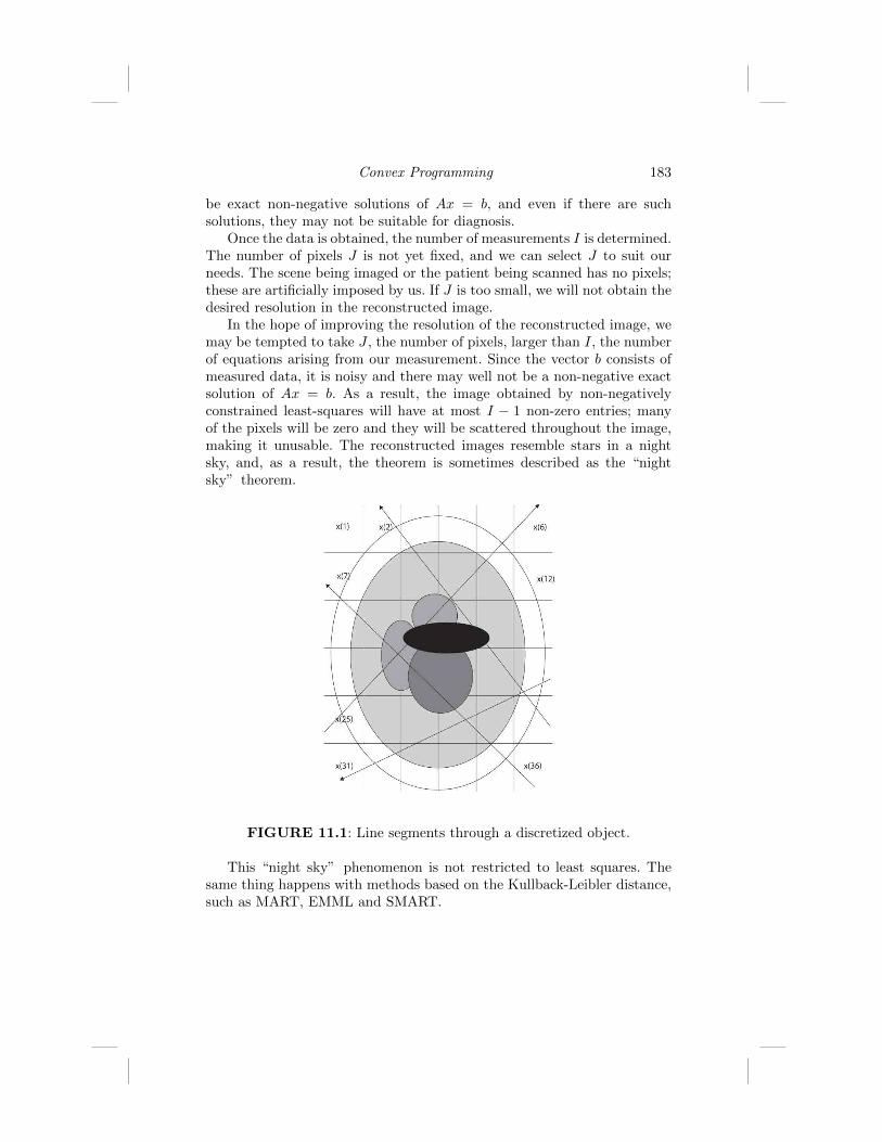
Convex Programming 183
be exact non-negative solutions of Ax = b, and even if there are suchsolutions, they may not be suitable for diagnosis.
Once the data is obtained, the number of measurements I is determined.The number of pixels J is not yet fixed, and we can select J to suit ourneeds. The scene being imaged or the patient being scanned has no pixels;these are artificially imposed by us. If J is too small, we will not obtain thedesired resolution in the reconstructed image.
In the hope of improving the resolution of the reconstructed image, wemay be tempted to take J , the number of pixels, larger than I, the numberof equations arising from our measurement. Since the vector b consists ofmeasured data, it is noisy and there may well not be a non-negative exactsolution of Ax = b. As a result, the image obtained by non-negativelyconstrained least-squares will have at most I − 1 non-zero entries; manyof the pixels will be zero and they will be scattered throughout the image,making it unusable. The reconstructed images resemble stars in a nightsky, and, as a result, the theorem is sometimes described as the “nightsky” theorem.
FIGURE 11.1: Line segments through a discretized object.
This “night sky” phenomenon is not restricted to least squares. Thesame thing happens with methods based on the Kullback-Leibler distance,such as MART, EMML and SMART.

184 A First Course in Optimization
11.12 Solving the Dual Problem
In this section we use the KKT Theorem to derive an iterative algorithmto minimize the function
f(x) =1
2‖x‖22,
subject to Ax ≥ b, by solving the dual problem of maximizing h(λ), overλ ≥ 0.
11.12.1 The Primal and Dual Problems
Minimizing f(x) over x such that Ax ≥ b is the primal problem. Herewe let gi = bi − (Ax)i, for i = 1, ..., I, and the set C be all of RJ . TheLagrangian is then
L(x, λ) =1
2||x||22 − λTAx+ λT b. (11.55)
The infimum of L(x, λ) over all x occurs when x = ATλ and so
h(λ) = λT b− 1
2||ATλ||22. (11.56)
For any x satisfying Ax ≥ b and any λ ≥ 0 we have h(λ) ≤ f(x). If x∗ isthe unique solution of the primal problem and λ∗ any solution of the dualproblem, we have f(x∗) = h(λ∗). The point here is that the constraintsin the dual problem are easier to implement in an iterative algorithm, sosolving the dual problem is the simpler task.
The algorithm we present now calculates iteratively two sequences, {xk}and {λk}, such that f(xk)−h(λk) converges to zero. The limits of {xk} and{λk} will be the solutions of the primal and dual problems, respectively.
11.12.2 Hildreth’s Dual Algorithm
The iterative algorithm we describe here was originally published byHildreth [128], and later extended by Lent and Censor [147]. It is a row-action method in that, at each step of the iteration, only a single row ofthe matrix A is used. Having found xk and λk, we use i = k(mod I) + 1,Ai the i-th row of A, and bi to calculate xk+1 and λk+1.
We know that the optimal x∗ and λ∗ ≥ 0 must satisfy x∗ = ATλ∗.Therefore, the algorithm guarantees that, at each step, we have λk > 0and xk = ATλk.
Having found xk and λk, we proceed as follows. First, we select i =

Convex Programming 185
k(mod I) + 1. Since
h(λ) = bTλ− 1
2‖ATλ‖22,
we have∇h(λ) = b−AATλ.
A gradient ascent method to maximize h(λ) would then have the iterativestep
λk+1 = λk + γk(b−AATλk) = λk + γk(b−Axk),
for some γk > 0. A row-action variant of gradient ascent modifies only thei-th entry of λ at the k-th step, with
λk+1i = λki + γk(bi − (Axk)i). (11.57)
Since we require that λk+1 ≥ 0, when (bi − (Axk)i) < 0 we must select γkso that
γk(bi − (Axk)i) ≥ −λki .
We then havexk+1 = xk + γk(bi − (Axk)i)A
Ti ,
which is used in the next step, in forming ∇h(λk+1). Proof of convergenceof this algorithm is presented in [83].
11.13 Minimum One-Norm Solutions
When the system of linear equations Ax = b is under-determined, itis common practice to seek a solution that also minimizes some objectivefunction. For example, the minimum two-norm solution is the vector xsatisfying Ax = b for which the (square of the) two-norm,
||x||22 =J∑j=1
x2j ,
is minimized. Alternatively, we may seek the minimum one-norm solution,for which the one-norm,
||x||1 =
J∑j=1
|xj |,
is minimized.If the vector x is required to be non-negative, then the one-norm is
simply the sum of the entries, and minimizing the one-norm subject to
186 A First Course in Optimization
Ax = b becomes a linear programming problem. This is the situation inapplications involving image reconstruction.
In compressed sampling [98] one seeks a solution of Ax = b havingrelatively few non-zero entries. The vector x here is not assumed to be non-negative, and the solution is found by minimizing the one-norm, subject tothe constraints Ax = b. The one-norm is not a linear functional of x, butthe problem can still be converted into a linear programming problem.
11.13.1 Reformulation as an LP Problem
The entries of x need not be non-negative, so the problem is not yet alinear programming problem. Let
B =[A −A
],
and consider the linear programming problem of minimizing the function
cT z =
2J∑j=1
zj ,
subject to the constraints z ≥ 0, and Bz = b. Let z∗ be the solution. Wewrite
z∗ =
[u∗
v∗
].
Then, as we shall see, x∗ = u∗ − v∗ minimizes the one-norm, subject toAx = b.
First, we show that u∗jv∗j = 0, for each j. If, say, there is a j such that
0 < v∗j ≤ u∗j , then we can create a new vector z from z∗ by replacing theold u∗j with u∗j − v∗j and the old v∗j with zero, while maintaining Bz = b.
But then, since u∗j − v∗j < u∗j + v∗j , it follows that cT z < cT z∗, which is a
contradiction. Consequently, we have ‖x∗‖1 = cT z∗.Now we select any x with Ax = b. Write uj = xj , if xj ≥ 0, and uj = 0,
otherwise. Let vj = uj − xj , so that x = u− v. Then let
z =
[uv
].
Then b = Ax = Bz, and cT z = ‖x‖1. Therefore
‖x∗‖1 = cT z∗ ≤ cT z = ‖x‖1,
and x∗ must be a minimum one-norm solution.The reader is invited to provide an example showing that a minimum
one-norm solution of Ax = b need not be unique.

Convex Programming 187
11.13.2 Image Reconstruction
In image reconstruction from limited linear-functional data, the vectorx is non-negative and arises as a vectorization of a two-dimensional image.The data we have pertaining to x is linear and takes the form Ax = b, forsome matrix A and vector b. Typically, the problem is under-determined,since the number of entries of x is the number of pixels in the image, whichwe can make as large as we wish. The problem then is to select, fromamong all the feasible images, one particular one that has a good chanceof being near the correct image. One approach is to take the solution ofAx = b having the minimum Euclidean norm, ||x||2. Algorithms such as theprojected ART and projected Landweber iterative methods can be used tofind such solutions.
Another approach is to find the non-negative solution of Ax = b forwhich the one-norm,
||x||1 =
J∑j=1
|xj |,
is minimized [98]. Since the xj are to be non-negative, the problem becomesthe following: minimize
f(x) =
J∑j=1
xj ,
subject togi(x) = (Ax)i − bi = 0,
for i = 1, ..., I, andgi(x) = −xi−I ≤ 0,
for i = I + 1, ..., I + J .When the system Ax = b is under-determined, the minimum one-norm
solution tends to be sparser than the minimum two-norm solution. A simpleexample will illustrate this point.
Consider the equation x+ 2y = 1. The minimum two-norm solution is
(0.2, 0.4), with two-norm√55 , which is about 0.4472, but one-norm equal
to 0.6. The solution (0, 0.5) has two-norm and one-norm equal to 0.5, andthe solution (1.0, 0) has two-norm and one-norm equal to 1.0. Therefore,the minimum one-norm solution is (0, 0.5), not (0.2, 0.4).
We can write the one-norm of the vector x as
||x||1 =
J∑j=1
|xj |2
|xj |.
The PDFT approach to image reconstruction [53] selects the solution of

188 A First Course in Optimization
Ax = b that minimizes the weighted two-norm
||x||2w =
J∑j=1
|xj |2
pj=
J∑j=1
|xj |2wj ,
where pj > 0 is a prior estimate of the non-negative image x to be recon-structed, and wj = p−1j . To the extent that pj accurately models the mainfeatures of x, such as which xj are nearly zero and which are not, the twoapproaches should give similar reconstructions. The PDFT can be imple-mented using the ART algorithm (see [188, 189, 190]). For more discussionof one-norm minimization, see the chapter on compressed sensing.
11.14 Exercises
Ex. 11.1 Prove Proposition 11.1.
Ex. 11.2 Prove Corollary 11.1.
Ex. 11.3 Show that, although K(1, 1) = 0, which is the saddle value, thepoint (1, 1) is not a saddle point for the function K(x, y) = x2 − y2.
Ex. 11.4 Prove Theorem 11.3.
Ex. 11.5 Apply the gradient form of the KKT Theorem to minimize thefunction f(x, y) = (x+ 1)2 + y2 over all x ≥ 0 and y ≥ 0.
Ex. 11.6 ([112]) Consider the following problem : minimize the function
f(x, y) = |x− 2|+ |y − 2|,
subject tog(x, y) = y2 − x ≤ 0,
andh(x, y) = x2 + y2 − 1 = 0.
Illustrate this problem graphically, showing lines of constant value of f andthe feasible region of points satisfying the constraints. Where is the solutionof the problem? Where is the solution, if the equality constraint is removed?Where is the solution, if both constraints are removed?
Convex Programming 189
Ex. 11.7 ([175], Ex. 5.2.9 (a)) Minimize the function
f(x, y) =√x2 + y2,
subject tox+ y ≤ 0.
Show that the function MP (z) is not differentiable at z = 0.
Ex. 11.8 ([175], Ex. 5.2.9 (b)) Minimize the function
f(x, y) = −2x− y,
subject tox+ y ≤ 1,
0 ≤ x ≤ 1,
andy ≥ 0.
Again, show that the function MP (z) is not differentiable at z = 0.
Ex. 11.9 (Duffin; [175], Ex. 5.2.9 (c)) Minimize the function
f(x, y) = e−y,
subject to √x2 + y2 − x ≤ 0.
Show that the function MP (z) is not continuous at z = 0.
Ex. 11.10 Apply the theory of convex programming to the primalQuadratic Programming Problem (QP), which is to minimize the function
f(x) =1
2xTQx,
subject toaTx ≤ c,
where a 6= 0 is in RJ , c < 0 is real, and Q is symmetric, and positive-definite.
Ex. 11.11 Use Theorem 11.6 to prove that any real N by N symmetricmatrix has N mutually orthonormal eigenvectors.


Chapter 12
Iterative Optimization
12.1 Chapter Summary . . . . . . . . . . . . . . . . . . . . . . . . . . . . . . . . . . . . . . . . . . . . . . . 19212.2 The Need for Iterative Methods . . . . . . . . . . . . . . . . . . . . . . . . . . . . . . . . . 19212.3 Optimizing Functions of a Single Real Variable . . . . . . . . . . . . . . . . . 193
12.3.1 Iteration and Operators . . . . . . . . . . . . . . . . . . . . . . . . . . . . . . . . . 19312.4 Descent Methods . . . . . . . . . . . . . . . . . . . . . . . . . . . . . . . . . . . . . . . . . . . . . . . . . 19412.5 Optimizing Functions of Several Real Variables . . . . . . . . . . . . . . . . . 19512.6 Projected Gradient-Descent Methods . . . . . . . . . . . . . . . . . . . . . . . . . . . . 196
12.6.1 Using Auxiliary-Function Methods . . . . . . . . . . . . . . . . . . . . . . 19812.6.2 Proving Convergence . . . . . . . . . . . . . . . . . . . . . . . . . . . . . . . . . . . . 199
12.7 The Newton-Raphson Approach . . . . . . . . . . . . . . . . . . . . . . . . . . . . . . . . . 20012.7.1 Functions of a Single Variable . . . . . . . . . . . . . . . . . . . . . . . . . . . 20012.7.2 Functions of Several Variables . . . . . . . . . . . . . . . . . . . . . . . . . . . 201
12.8 Approximate Newton-Raphson Methods . . . . . . . . . . . . . . . . . . . . . . . . 20212.8.1 Avoiding the Hessian Matrix . . . . . . . . . . . . . . . . . . . . . . . . . . . . 202
12.8.1.1 The BFGS Method . . . . . . . . . . . . . . . . . . . . . . . . 20212.8.1.2 The Broyden Class . . . . . . . . . . . . . . . . . . . . . . . . . 203
12.8.2 Avoiding the Gradient . . . . . . . . . . . . . . . . . . . . . . . . . . . . . . . . . . . 20312.9 Derivative-Free Methods . . . . . . . . . . . . . . . . . . . . . . . . . . . . . . . . . . . . . . . . . 203
12.9.1 Multi-directional Search Algorithms . . . . . . . . . . . . . . . . . . . . 20412.9.2 The Nelder-Mead Algorithm . . . . . . . . . . . . . . . . . . . . . . . . . . . . 20412.9.3 Comments on the Nelder-Mead Algorithm . . . . . . . . . . . . . . 205
12.10 Rates of Convergence . . . . . . . . . . . . . . . . . . . . . . . . . . . . . . . . . . . . . . . . . . . . 20512.10.1 Basic Definitions . . . . . . . . . . . . . . . . . . . . . . . . . . . . . . . . . . . . . . . . . 20512.10.2 Illustrating Quadratic Convergence . . . . . . . . . . . . . . . . . . . . . 20512.10.3 Motivating the Newton-Raphson Method . . . . . . . . . . . . . . . 206
12.11 Feasible-Point Methods . . . . . . . . . . . . . . . . . . . . . . . . . . . . . . . . . . . . . . . . . . 20612.11.1 The Projected Gradient Algorithm . . . . . . . . . . . . . . . . . . . . . 20712.11.2 Reduced Gradient Methods . . . . . . . . . . . . . . . . . . . . . . . . . . . . . 20712.11.3 The Reduced Newton-Raphson Method . . . . . . . . . . . . . . . . 208
12.11.3.1 An Example . . . . . . . . . . . . . . . . . . . . . . . . . . . . . . . . 20812.11.4 A Primal-Dual Approach . . . . . . . . . . . . . . . . . . . . . . . . . . . . . . . . 209
12.12 Simulated Annealing . . . . . . . . . . . . . . . . . . . . . . . . . . . . . . . . . . . . . . . . . . . . . 21012.13 Exercises . . . . . . . . . . . . . . . . . . . . . . . . . . . . . . . . . . . . . . . . . . . . . . . . . . . . . . . . . 211
191

192 A First Course in Optimization
12.1 Chapter Summary
Now we begin our discussion of iterative methods for solving optimiza-tion problems. Topics include the role of the gradient operator, the Newton-Raphson (NR) method, and various computationally simpler variants of theNR method.
12.2 The Need for Iterative Methods
We know from beginning calculus that, if we want to optimize a differ-entiable function g(x) of a single real variable x, we begin by finding theplaces where the derivative is zero, g′(x) = 0. Similarly, if we want to opti-mize a differentiable function g(x) of a real vector variable x, we begin byfinding the places where the gradient is zero, ∇g(x) = 0. Generally, though,this is not the end of the story, for we still have to solve an equation forthe optimal x. Unless we are fortunate, solving this equation algebraicallymay be computationally expensive, or may even be impossible, and we willneed to turn to iterative methods. This suggests that we might use iterativemethods to minimize g(x) directly, and not solve an equation.
For example, suppose we wish to solve the over-determined system oflinear equations Ax = b, but we don’t know if the system has solutions. Inthat case, we may wish to minimize the function
g(x) =1
2‖Ax− b‖22,
to get a least-squares solution. We know from linear algebra that if thematrix ATA is invertible, then the unique minimizer of g(x) is given by
x∗ = (ATA)−1AT b.
In many applications, the number of equations and the number of unknownsmay be quite large, making it expensive even to calculate the entries of thematrix ATA. In such cases, we can find x∗ using an iterative method suchas Landweber’s Algorithm, which has the iterative step
xk+1 = xk + γAT (b−Axk).
The sequence {xk} converges to x∗ for any value of γ in the interval(0, 2/λmax), where λmax is the largest eigenvalue of the matrix ATA.

Iterative Optimization 193
12.3 Optimizing Functions of a Single Real Variable
Suppose g : R→ R is differentiable and attains its minimum value. Wewant to minimize the function g(x). Solving g′(x) = 0 to find the optimalx = x∗ may not be easy, so we may turn to an iterative algorithm forfinding roots of g′(x), or one that minimizes g(x) directly. In the lattercase, we may consider an iterative procedure
xk+1 = xk − γkg′(xk), (12.1)
for some sequence {γk} of positive numbers. Such iterative procedures arecalled descent algorithms because, if g′(xk) > 0, then we want to move tothe left of xk, while, if g′(xk) < 0, we want to move to the right.
We shall be particularly interested in algorithms in which γk = γ forall k. We denote by T the operator
Tx = x− γg′(x). (12.2)
Then, using g′(x∗) = 0, we find that
|x∗ − xk+1| = |Tx∗ − Txk|. (12.3)
12.3.1 Iteration and Operators
The iterative methods we shall consider involve the calculation of asequence {xk} of vectors in RJ , according to the formula xk+1 = Txk,where T is some function T : RJ → RJ ; such functions are called operatorson RJ . The operator Tx = x− g′(x) above is an operator on R.
Definition 12.1 An operator T on RJ is continuous at x in the interiorof its domain if
limz→x‖Tz − Tx‖ = 0.
All the operators we shall consider are continuous.The sequences generated by iterative methods can then be written
{T kx0}, where x = x0 is the starting point for the iteration and T k meansapply the operator T k times. If the sequence {xk} converges to a limitvector x in the domain of T , then, taking the limit, as k → +∞, on bothsides of
xk+1 = Txk,
and using the continuity of the operator T , we have
x = T x,
that is, the limit vector x is a fixed point of T .

194 A First Course in Optimization
Definition 12.2 A vector x in the domain of the operator T is a fixedpoint of T if T x = x. The set of all fixed points of T is denoted Fix(T ).
We have several concerns, when we use iterative methods:
• Does the operator T have any fixed points?
• Does the sequence {T kx0} converge?
• Does convergence depend on the choice of x0?
• When the sequence {T kx0} converges, is the limit a solution to ourproblem?
• How fast does the sequence {T kx0} converge?
• How difficult is it to perform a single step, going from xk to xk+1?
• How does the limit depend on the starting vector x0?
To answer these questions, we will need to learn about the properties ofthe particular operator T being used. We begin our study of iterative op-timization algorithms with the gradient descent methods, particularly asthey apply to convex functions.
12.4 Descent Methods
Suppose that g(x) is convex and the function f(x) = g′(x) is L-Lipschitz. If g(x) is twice differentiable, this would be the case if
0 ≤ g′′(x) ≤ L, (12.4)
for all x. If γ is in the interval (0, 2L ), then the operator Tx = x − γg′(x)
is an averaged operator; from the KMO Theorem 15.2, we know that theiterative sequence {T kx0} converges to a minimizer of g(x), whenever aminimizer exists.
If g(x) is convex and f(x) = g′(x) is L-Lipschitz, then 1Lg′(x) is non-
expansive, so that, by Theorem 10.20 1Lg′(x) is fne and g′(x) is 1
L -ism.Then, as we shall see later, the operator
Tx = x− γg′(x) (12.5)
is av whenever 0 < γ < 2L , and so the iterative sequence xk+1 = Txk =
xk − γg′(xk) converges to a minimizer of g(x), whenever minimizers exist.In the next section we extend these results to functions of several vari-
ables.
Iterative Optimization 195
12.5 Optimizing Functions of Several Real Variables
Suppose g : RJ → R is differentiable and attains its minimum value. Wewant to minimize the function g(x). Solving ∇g(x) = 0 to find the optimalx = x∗ may not be easy, so we may turn to an iterative algorithm forfinding roots of ∇g(x), or one that minimizes g(x) directly. From Cauchy’sInequality, we know that the directional derivative of g(x), at x = a, andin the direction of the vector unit vector d, satisfies
|g′(a; d)| = |〈∇g(a), d〉| ≤ ‖∇g(a)‖2 ‖d‖2,
and that g′(a; d) attains its most positive value when the direction d is apositive multiple of ∇g(a). This suggests steepest descent optimization.
Steepest descent iterative optimization makes use of the fact that thedirection of greatest increase of g(x) away from x = xk is in the directiond = ∇g(xk). Therefore, we select as the next vector in the iterative sequence
xk+1 = xk − γk∇g(xk), (12.6)
for some γk > 0. Ideally, we would choose γk optimally, so that
g(xk − γk∇g(xk)) ≤ g(xk − γ∇g(xk)), (12.7)
for all γ ≥ 0; that is, we would proceed away from xk, in the direction of−∇g(xk), stopping just as g(x) begins to increase. Then we call this pointxk+1 and repeat the process.
Lemma 12.1 Suppose that xk+1 is chosen using the optimal value of γk,as described by Equation (12.7). Then
〈∇g(xk+1),∇g(xk)〉 = 0. (12.8)
In practice, finding the optimal γk is not a simple matter. Instead, onecan try a few values of α and accept the best of these few, or one can tryto find a constant value γ of the parameter having the property that theiterative step
xk+1 = xk − γ∇g(xk)
leads to a convergent sequence. It is this latter approach that we shallconsider here.
We denote by T the operator
Tx = x− γ∇g(x). (12.9)
Then, using ∇g(x∗) = 0, we find that
‖x∗ − xk+1‖2 = ‖Tx∗ − Txk‖2. (12.10)
196 A First Course in Optimization
We would like to know if there are choices for γ that imply convergence ofthe iterative sequence. As in the case of functions of a single variable, forfunctions g(x) that are convex, the answer is yes.
If g(x) is convex and F (x) = ∇g(x) is L-Lipschitz, then G(x) = 1L∇g(x)
is firmly non-expansive. Then, as we shall see later, for γ > 0, the operator
Tx = x− γ∇g(x) (12.11)
is averaged, whenever 0 < γ < 2L . It follows from the KMO Theorem 15.2
that the iterative sequence xk+1 = Txk = xk − γ∇g(xk) converges to aminimizer of g(x), whenever minimizers exist.
For example, the function g(x) = 12‖Ax− b‖
22 is convex and its gradient
isf(x) = ∇g(x) = AT (Ax− b).
A steepest descent algorithm for minimizing g(x) then has the iterativestep
xk+1 = xk − γkAT (Axk − b),where the parameter γk should be selected so that
g(xk+1) < g(xk).
The linear operator that transforms each vector x into ATAx has the prop-erty that
‖ATAx−ATAy‖2 ≤ λmax‖x− y‖2,where λmax is the largest eigenvalue of the matrix ATA; this operator isthen L-Lipschitz, for L = λmax. Consequently, the operator that transformsx into 1
LATAx is non-expansive.
12.6 Projected Gradient-Descent Methods
As we have remarked previously, one of the fundamental problems incontinuous optimization is to find a minimizer of a function over a subset ofRJ .The following propositions will help to motivate the projected gradient-descent algorithm.
Proposition 12.1 Let f : RJ → R be convex and differentiable and letC ⊆ RJ be closed, non-empty and convex. Then x ∈ C minimizes f overC if and only if
〈∇f(x), c− x〉 ≥ 0, (12.12)
for all c ∈ C.
Iterative Optimization 197
Proof: Since f is convex, we know from Theorem 10.16 that
f(b)− f(a) ≥ 〈∇f(a), b− a〉 ,
for all a and b. Therefore, if
〈∇f(x), c− x〉 ≥ 0,
for all c ∈ C, then f(c)− f(x) ≥ 0 for all c ∈ C also.Conversely, suppose that f(c)− f(x) ≥ 0, for all c ∈ C. For each c ∈ C,
let d = c−x‖c−x‖2 , so that
〈∇f(x), d〉 =1
‖c− x‖2〈∇f(x), c− x〉
is the directional derivative of f at x, in the direction of c. Because f(c)−f(x) ≥ 0, for all c ∈ C, this directional derivative must be non-negative.
Proposition 12.2 Let f : RJ → R be convex and differentiable and letC ⊆ RJ be closed, non-empty and convex. Then x ∈ C minimizes f overC if and only if
x = PC(x− γ∇f(x)),
for all γ > 0.
Proof: By Proposition 6.4, we know that x = PC(x− γ∇f(x)) if and onlyif
〈x− (x− γ∇f(x)), c− x〉 ≥ 0,
for all c ∈ C. But this is equivalent to
〈∇f(x), c− x〉 ≥ 0,
for all c ∈ C, which, by the previous proposition, is equivalent to x mini-mizing the function f over all c ∈ C.
This leads us to the projected gradient-descent algorithm. According tothe previous proposition, we know that x minimizes f over C if and onlyif x is a fixed point of the operator
Tx = PC(x− γ∇f(x)).
We provide an elementary proof of the following theorem:
Theorem 12.1 Let f : RJ → R be convex and differentiable, with ∇fL-Lipschitz. Let C be any closed, convex subset of RJ . For 0 < γ < 1
L , letT = PC(I − γ∇f). If T has fixed points, then the sequence {xk} given byxk = Txk−1 converges to a fixed point of T , which is then a minimizer off over C.

198 A First Course in Optimization
The iterative step is given by
xk = PC(xk−1 − γ∇f(xk−1)). (12.13)
Any fixed point of the operator T minimizes the function f(x) over x in C.It is a consequence of the KMO Theorem 15.2 for averaged operators
that convergence holds for 0 < γ < 2L . The proof given here employs
sequential unconstrained minimization and avoids using the non-trivial re-sults that, because the operator 1
L∇f is non-expansive, it is firmly non-expansive (see Theorem 10.20), and that the product of averaged operatorsis again averaged (see Proposition 15.1).
12.6.1 Using Auxiliary-Function Methods
We can use auxiliary-function (AF) methods to prove Theorem 12.1.For each k = 1, 2, ... let
Gk(x) = f(x) +1
2γ‖x− xk−1‖22 −Df (x, xk−1), (12.14)
where
Df (x, xk−1) = f(x)− f(xk−1)− 〈∇f(xk−1), x− xk−1〉. (12.15)
Since f(x) is convex, Df (x, y) ≥ 0 for all x and y and is the Bregmandistance formed from the function f [25].
The auxiliary function
gk(x) =1
2γ‖x− xk−1‖22 −Df (x, xk−1) (12.16)
can be rewritten as
gk(x) = Dh(x, xk−1), (12.17)
where
h(x) =1
2γ‖x‖22 − f(x). (12.18)
Therefore, gk(x) ≥ 0 whenever h(x) is a convex function.We know that h(x) is convex if and only if
〈∇h(x)−∇h(y), x− y〉 ≥ 0, (12.19)
for all x and y. This is equivalent to
1
γ‖x− y‖22 − 〈∇f(x)−∇f(y), x− y〉 ≥ 0. (12.20)
Since ∇f is L-Lipschitz, the inequality (12.20) holds whenever 0 < γ < 1L .

Iterative Optimization 199
Lemma 12.2 The xk that minimizes Gk(x) over x ∈ C is given by Equa-tion (12.13).
Proof: We know that
〈∇Gk(xk), x− xk〉 ≥ 0,
for all x ∈ C. With
∇Gk(xk) =1
γ(xk − xk−1) +∇f(xk−1),
we have〈xk − (xk−1 − γ∇f(xk−1)), x− xk〉 ≥ 0,
for all x ∈ C. We then conclude that
xk = PC(xk−1 − γ∇f(xk−1)).
12.6.2 Proving Convergence
A relatively simple calculation shows that
Gk(x)−Gk(xk) =1
2γ‖x− xk‖22 +
1
γ〈xk − (xk−1 − γ∇f(xk−1)), x− xk〉.
(12.21)
From Equation (12.13) it follows that
Gk(x)−Gk(xk) ≥ 1
2γ‖x− xk‖22, (12.22)
for all x ∈ C, so that
Gk(x)−Gk(xk) ≥ 1
2γ‖x− xk‖22 −Df (x, xk) = gk+1(x). (12.23)
Now let x minimize f(x) over all x ∈ C. Then
Gk(x)−Gk(xk) = f(x) + gk(x)− f(xk)− gk(xk)
≤ f(x) +Gk−1(x)−Gk−1(xk−1)− f(xk)− gk(xk),
so that(Gk−1(x)−Gk−1(xk−1)
)−(Gk(x)−Gk(xk)
)≥ f(xk)−f(x)+gk(xk) ≥ 0.

200 A First Course in Optimization
Therefore, the sequence {Gk(x)−Gk(xk)} is decreasing and the sequences{gk(xk)} and {f(xk)− f(x)} converge to zero.
From
Gk(x)−Gk(xk) ≥ 1
2γ‖x− xk‖22,
it follows that the sequence {xk} is bounded. Let {xkn} converge to x∗ ∈ Cwith {xkn+1} converging to x∗∗ ∈ C; we then have f(x∗) = f(x∗∗) = f(x).
Replacing the generic x with x∗∗, we find that {Gkn+1(x∗∗) −Gkn+1(xkn+1)} is decreasing. By Equation (12.21), this subsequence con-verges to zero; therefore, the entire sequence {Gk(x∗∗)−Gk(xk)} convergesto zero. From the inequality in (12.22), we conclude that the sequence{‖x∗∗ − xk‖22} converges to zero, and so {xk} converges to x∗∗. This com-pletes the proof of the theorem.
12.7 The Newton-Raphson Approach
The Newton-Raphson approach to minimizing a real-valued functionf : RJ → R involves finding x∗ such that ∇f(x∗) = 0.
12.7.1 Functions of a Single Variable
We begin with the problem of finding a root of a function g : R→ R. Ifx0 is not a root, compute the line tangent to the graph of g at x = x0 andlet x1 be the point at which this line intersects the horizontal axis; that is,
x1 = x0 − g(x0)/g′(x0). (12.24)
Continuing in this fashion, we have
xk+1 = xk − g(xk)/g′(xk). (12.25)
This is the Newton-Raphson algorithm for finding roots. Convergence, whenit occurs, is usually more rapid than gradient descent, but requires that x0
be sufficiently close to the solution.Now suppose that f : R → R is a real-valued function that we wish
to minimize by solving f ′(x) = 0. Letting g(x) = f ′(x) and applying theNewton-Raphson algorithm to g(x) gives the iterative step
xk+1 = xk − f ′(xk)/f ′′(xk). (12.26)
This is the Newton-Raphson optimization algorithm. Now we extend theseresults to functions of several variables.

Iterative Optimization 201
12.7.2 Functions of Several Variables
The Newton-Raphson algorithm for finding roots of functions g : RJ →RJ has the iterative step
xk+1 = xk − [J (g)(xk)]−1g(xk), (12.27)
where J (g)(x) is the Jacobian matrix of first partial derivatives, ∂gm∂xj(xk),
for g(x) = (g1(x), ..., gJ(x))T .To minimize a function f : RJ → R, we let g(x) = ∇f(x) and find a
root of g. Then the Newton-Raphson iterative step becomes
xk+1 = xk − [∇2f(xk)]−1∇f(xk), (12.28)
where∇2f(x) = J (g)(x) is the Hessian matrix of second partial derivativesof f .
The quadratic approximation to f(x) around the point xk is
f(x) ≈ f(xk) + 〈∇f(xk), x− xk〉+1
2(x− xk)T∇2f(xk)(x− xk).
The right side of this equation attains its minimum value when
0 = ∇f(xk) +∇2f(xk)(x− xk),
that is, when x = xk+1 as given by Equation (12.28).If f(x) is a quadratic function, that is,
f(x) = xTQx+ xT b+ c,
for constant invertible matrix Q and constant vectors b and c, then theNewton-Raphson iteration converges to the answer in one step. Therefore,if f(x) is close to quadratic, the convergence should be reasonably rapid.This leads to the notion of self-concordant functions, for which the thirdderivative of f(x) is small, relative to the second derivative [163].
From the quadratic approximation
f(xk+1) ≈ f(xk)+〈∇f(xk), xk+1−xk〉+ 1
2(xk+1−xk)T∇2f(xk)(xk+1−xk),
and the formula for the iterative NR step we find that
f(xk+1)− f(xk) ≈ −1
2∇f(xk)T [∇2f(xk)]−1∇f(xk).
If the Hessian matrix ∇2f(xk) is always positive-definite, which may notbe the case, then its inverse will also be positive-definite and the NR stepwill reduce the value of the objective function f(x). One area of researchin the intersection of numerical linear algebra and optimization focuses onfinding positive-definite approximations of the Hessian matrix [202].

202 A First Course in Optimization
12.8 Approximate Newton-Raphson Methods
To use the NR method to minimize f(x), at each step of the iterationwe need to solve a system of equations involving the Hessian matrix for f .There are many iterative procedures designed to retain much of the advan-tages of the NR method, while avoiding the use of the Hessian matrix, or,indeed, while avoiding the use of the gradient. These methods are discussedin most texts on numerical methods [163]. We sketch briefly some of theseapproaches.
12.8.1 Avoiding the Hessian Matrix
Quasi-Newton methods, designed to avoid having to calculate the Hes-sian matrix, are often used instead of the Newton-Raphson algorithm. Theiterative step of the quasi-Newton methods is
xk+1 = xk −B−1k ∇f(xk), (12.29)
where the matrix Bk is an approximation of ∇2f(xk) that is easier tocompute.
In the case of g : R→ R, the second derivative of g(x) is approximately
g′′(xk) ≈ g′(xk)− g′(xk−1)
xk − xk−1. (12.30)
This suggests that, for the case of functions of several variables, the matrixBk should be selected so that
Bk(xk − xk−1) = ∇f(xk)−∇f(xk−1). (12.31)
In addition to satisfying Equation (12.31), the matrix Bk should also besymmetric and positive-definite. Finally, we should be able to obtain Bk+1
relatively easily from Bk.
12.8.1.1 The BFGS Method
The Broyden, Fletcher, Goldfarb, and Shanno (BFGS) method uses therank-two update formula
Bk+1 = Bk −(Bks
k)(Bksk)T
(sk)TBksk+yk(yk)T
(yk)T sk, (12.32)
with
sk = xk+1 − xk, (12.33)

Iterative Optimization 203
and
yk = ∇f(xk+1)−∇f(xk). (12.34)
12.8.1.2 The Broyden Class
A general class of update methods, known as the Broyden class, usesthe update formula
Bk+1 = Bk −(Bks
k)(Bksk)T
(sk)TBksk+yk(yk)T
(yk)T sk+ φ((sk)TBks
k)uk(uk)T ,(12.35)
with φ a scalar and
uk =yk
(yk)T sk− Bks
k
(sk)TBksk. (12.36)
When φ = 0 we get the BFGS method, while the choice of φ = 1 gives theDavidon, Fletcher, and Powell (DFP) method.
Note that for the updates in the Broyden class, the matrix Bk+1 hasthe form
Bk+1 = Bk + ak(ak)T + bk(bk)T + ck(ck)T ,
for certain vectors ak, bk and ck. Therefore, the inverse of Bk+1 can be ob-tained easily from the inverse of Bk, with three applications of the Sherman-Morrison-Woodbury Identity (see Exercise 8.4).
12.8.2 Avoiding the Gradient
Quasi-Newton methods use an approximation of the Hessian matrixthat is simpler to calculate, but still employ the gradient at each step.For functions g : R → R, the derivative can be approximated by a finitedifference, that is,
g′(xk) ≈ g(xk)− g(xk−1)
xk − xk−1. (12.37)
In the case of functions of several variables, the gradient vector can beapproximated by using a finite-difference approximation for each of thefirst partial derivatives.
12.9 Derivative-Free Methods
In many important applications, calculating values of the function tobe optimized is expensive and calculating gradients impractical. In such

204 A First Course in Optimization
cases, it is common to use direct-search methods. Generally, these are iter-ative methods that are easy to program, do not employ derivatives or theirapproximations, require relatively few function evaluations, and are usefuleven when the measurements are noisy.
12.9.1 Multi-directional Search Algorithms
Methods such as the multi-directional search algorithms begin with thevalues of the function f(x) at J + 1 points, where x is in RJ , and thenuse these values to move to a new set of points. These points are chosento describe a simplex pattern in RJ , that is, they do not all lie on a singlehyperplane in RJ . For that reason, these methods are sometimes calledsimplex methods, although they are unrelated to Dantzig’s method of thesame name. The Nelder-Mead algorithm [164, 142, 155] is one such simplexalgorithm.
12.9.2 The Nelder-Mead Algorithm
For simplicity, we follow McKinnon [155] and describe the Nelder-Mead(NM) algorithm only for the case of J = 2. The NM algorithm begins withthe choice of vertices:
ORDER: obtain b, s, and w, with
f(b) ≤ f(s) ≤ f(w).
Then take
m =1
2(b+ s).
Let the search line be
L(ρ) = m+ ρ(m− w),
andr = L(1) = 2m− w.
• {if f(r) < f(b)} let e = L(2). If f(e) < f(b) accept e; otherwiseaccept r.
• {if f(b) ≤ f(r)} then
– {if f(r) < f(s)} accept r.
– {if f(s) ≤ f(r)}∗ {if f(r) < f(w)} let c = L(0.5)
· {if f(c) ≤ f(r)} accept c;
Iterative Optimization 205
· {if f(r) < f(c)} go to SHRINK.
∗ {if f(w) ≤ f(r)} let c = L(−0.5).
· {if f(c) < f(w)} accept c; otherwise go to SHRINK.
Replace w with the accepted point and go to ORDER.SHRINK: Replace s with 1
2 (s+ b) and w with 12 (w + b); go to ORDER.
12.9.3 Comments on the Nelder-Mead Algorithm
Although the Nelder-Mead algorithm is quite popular in many areas ofapplications, relatively little of a theoretical nature is known. The interestedreader is directed to the papers [142, 155], as well as to more recent work byMargaret Wright of NYU. A good treatment of the Nelder-Mead algorithm,along with a number of other derivative-free techniques, is the new bookby Conn, Scheinberg and Vicente [89].
12.10 Rates of Convergence
In this section we illustrate the concept of rate of convergence [30] byconsidering the fixed-point iteration xk+1 = g(xk), for the twice continu-ously differentiable function g : R→ R. We suppose that g(z) = z and weare interested in the distance |xk − z|.
12.10.1 Basic Definitions
Definition 12.3 Suppose the sequence {xk} converges to z. If there arepositive constants λ and α such that
limk→∞
|xk+1 − z||xk − z|α
= λ, (12.38)
then {xk} is said to converge to z with order α and asymptotic error con-stant λ. If α = 1, the convergence is said to be linear; if α = 2, the conver-gence is said to be quadratic.
12.10.2 Illustrating Quadratic Convergence
According to the Extended Mean Value Theorem,
g(x) = g(z) + g′(z)(x− z) +1
2g′′(c)(x− z)2, (12.39)

206 A First Course in Optimization
for some c between x and z. Suppose now that xk → z and, in addition,g′(z) = 0. Then we have
xk+1 = g(xk) = z +1
2g′′(ck)(xk − z)2, (12.40)
for some ck between xk and z. Therefore,
|xk+1 − z| =1
2|g′′(ck)| |xk − z|2, (12.41)
and the convergence is quadratic, with λ = |g′′(z)|.
12.10.3 Motivating the Newton-Raphson Method
Suppose that we are seeking a root z of the function f : R → R. Wedefine
g(x) = x− h(x)f(x), (12.42)
for some function h(x) to be determined. Then f(z) = 0 implies thatg(z) = z. In order to have quadratic convergence of the iterative sequencexk+1 = g(xk), we want g′(z) = 0. From
g′(x) = 1− h′(x)f(x)− h(x)f ′(x), (12.43)
it follows that we want
h(z) = 1/f ′(z). (12.44)
Therefore, we choose
h(x) = 1/f ′(x), (12.45)
so that
g(x) = x− f(x)/f ′(x). (12.46)
The iteration then takes the form
xk+1 = g(xk) = xk − f(xk)/f ′(xk), (12.47)
which is the Newton-Raphson iteration.
12.11 Feasible-Point Methods
We consider now the problem of minimizing the function f(x) : RJ → R,subject to the equality constraints Ax = b, where A is an I by J real matrix,with rank I and I < J . The methods we consider here are feasible-pointmethods, also called interior-point methods.

Iterative Optimization 207
12.11.1 The Projected Gradient Algorithm
Let C be the set of all x in RJ such that Ax = b. For every z in RJ , wehave
PCz = PNS(A)z +AT (AAT )−1b, (12.48)
where NS(A) is the null space of A. Using
PNS(A)z = z −AT (AAT )−1Az, (12.49)
we have
PCz = z +AT (AAT )−1(b−Az). (12.50)
The iteration in Equation (12.13) becomes
ck = ck−1 − γPNS(A)∇f(ck−1), (12.51)
which converges to a solution for any γ in (0, 1L ), whenever solutions exist.
We call this method the projected gradient algorithm.In the next subsection we present a somewhat simpler approach.
12.11.2 Reduced Gradient Methods
Let c0 be a feasible point, that is, Ac0 = b. Then c = c0 + p is alsofeasible if p is in the null space of A, that is, Ap = 0. Let Z be a J byJ − I matrix whose columns form a basis for the null space of A. We wantp = Zv for some v. The best v will be the one for which the function
φ(v) = f(c0 + Zv)
is minimized. We can apply to the function φ(v) the steepest descentmethod, or Newton-Raphson or any other minimization technique.
The steepest descent method, applied to φ(v), is called the reducedsteepest descent method [163]. The gradient of φ(v), also called the reducedgradient, is
∇φ(v) = ZT∇f(c),
where c = c0 + Zv. We choose the matrix Z so that ρ(ZTZ) ≤ 1, so thatthe gradient operator ∇φ is L-Lipschitz.
For the reduced gradient algorithm, the iteration in Equation (12.13)becomes
vk = vk−1 − γ∇φ(vk−1), (12.52)
so that the iteration for ck = c0 + Zvk is
ck = ck−1 − γZZT∇f(ck−1). (12.53)
The vectors ck are feasible and the sequence {ck} converges to a solution,whenever solutions exist, for any 0 < γ < 1
L .

208 A First Course in Optimization
12.11.3 The Reduced Newton-Raphson Method
The next method we consider is a modification of the Newton-Raphsonmethod, in which we begin with a feasible point and each NR step is inthe null space of the matrix A, to maintain the condition Ax = b. Thediscussion here is taken from [163].
Once again, our objective is to minimize φ(v). The Newton-Raphsonmethod, applied to φ(v), is called the reduced Newton-Raphson method.The Hessian matrix of φ(v), also called the reduced Hessian matrix, is
∇2φ(v) = ZT∇2f(x)Z,
where x = x+Zv, so algorithms to minimize φ(v) can be written in termsof the gradient and Hessian of f itself.
The reduced NR algorithm can then be viewed in terms of the vectors{vk}, with v0 = 0 and
vk+1 = vk − [∇2φ(vk)]−1∇φ(vk); (12.54)
the corresponding xk isxk = x+ Zvk.
12.11.3.1 An Example
Consider the problem of minimizing the function
f(x) =1
2x21 −
1
2x23 + 4x1x2 + 3x1x3 − 2x2x3,
subject tox1 − x2 − x3 = −1.
Let x = [1, 1, 1]T . Then the matrix A is A = [1,−1,−1] and the vector b isb = [−1]. Let the matrix Z be
Z =
1 11 00 1
. (12.55)
The reduced gradient at x is then
ZT∇f(x) =
[1 1 01 0 1
]820
=
[108
], (12.56)
and the reduced Hessian matrix at x is
ZT∇2f(x)Z =
[1 1 01 0 1
]1 4 34 0 −23 −2 −1
1 11 00 1
=
[9 66 6
]. (12.57)

Iterative Optimization 209
Then the reduced Newton-Raphson equation yields
v =
[−2/3−2/3
], (12.58)
and the reduced Newton-Raphson direction is
p = Zv =
−4/3−2/3−2/3
. (12.59)
Since the function φ(v) is quadratic, one reduced Newton-Raphson stepsuffices to obtain the solution, x∗ = [−1/3, 1/3, 1/3]T .
12.11.4 A Primal-Dual Approach
Once again, the objective is to minimize the function f(x) : RJ → R,subject to the equality constraints Ax = b. According to the Karush-Kuhn-Tucker Theorem 11.5, ∇L(x, λ) = 0 at the optimal values of x and λ, wherethe Lagrangian L(x, λ) is
L(x, λ) = f(x) + λT (b−Ax).
Finding a zero of the gradient of L(x, λ) means that we have to solve theequations
∇f(x)−ATλ = 0
andAx = b.
We define the function G(x, λ) taking values in RJ × RI to be
G(x, λ) = (∇f(x)−ATλ,Ax− b)T .
We then apply the NR method to find a zero of the function G. The Jaco-bian matrix for G is
JG(x, λ) =
[∇2f(x) −ATA 0
],
so one step of the NR method is
(xk+1, λk+1)T = (xk, λk)T − JG(xk, λk)−1G(xk, λk). (12.60)
We can rewrite this as
∇2f(xk)(xk+1 − xk)−AT (λk+1 − λk) = ATλk −∇f(xk), (12.61)

210 A First Course in Optimization
and
A(xk+1 − xk) = b−Axk. (12.62)
It follows from Equation (12.62) that Axk+1 = b, for k = 0, 1, ... , so thatthis primal-dual algorithm is a feasible-point algorithm.
In Quadratic Programming the Equations 12.61 and 12.62 producedby each step of the NR method are also precisely the conditions that theKKT Theorem gives for a solution to a particular quadratic-programmingproblem. Since every quadratic-programming problem can be reformulatedas a linear programming problem, each step of the primal-dual iterationcan be computed using the simplex algorithm. This primal-dual algorithmcan be used to solve linear-programming problems.
12.12 Simulated Annealing
In this chapter we have focused on the minimization of convex functions.For such functions, a local minimum is necessarily a global one. For non-convex functions, this is not the case. For example, the function f(x) =x4 − 8x3 + 20x2 − 16.5x + 7 has a local minimum around x = 0.6 and aglobal minimum around x = 3.5. The descent methods we have discussedcan get caught at a local minimum that is not global, since we insist onalways taking a step that reduces f(x). The simulated annealing algorithm[1, 157], also called the Metropolis algorithm, is sometimes able to avoidbeing trapped at a local minimum by permitting an occasional step thatincreases f(x). The name comes from the analogy with the physical problemof lowering the energy of a solid by first raising the temperature, to bringthe particles into a disorganized state, and then gradually reducing thetemperature, so that a more organized state is achieved.
Suppose we have calculated xk. We now generate a random directionand a small random step length. If the new vector xk + ∆x makes f(x)smaller, we accept the vector as xk+1. If not, then we accept this vector,with probability
Prob(accept) = exp(f(xk)− f(xk + ∆x)
ck
),
where ck > 0, known as the temperature, is chosen by the user. As the iter-ation proceeds, the temperature ck is gradually reduced, making it easierto accept increases in f(x) early in the process, but harder later. How toselect the temperatures is an art, not a science.

Iterative Optimization 211
12.13 Exercises
Ex. 12.1 Prove Lemma 12.1.
Ex. 12.2 Apply the Newton-Raphson method to obtain an iterative pro-cedure for finding
√a, for any positive a. For which x0 does the method
converge? There are two answers, of course; how does the choice of x0
determine which square root becomes the limit?
Ex. 12.3 Apply the Newton-Raphson method to obtain an iterative proce-dure for finding a1/3, for any real a. For which x0 does the method converge?
Ex. 12.4 Extend the Newton-Raphson method to complex variables. Redothe previous exercises for the case of complex a. For the complex case, ahas two square roots and three cube roots. How does the choice of x0 affectthe limit? Warning: The case of the cube root is not as simple as it mayappear, and has a close connection to fractals and chaos; see [185].
Ex. 12.5 Use the reduced Newton-Raphson method to minimize the func-tion 1
2xTQx, subject to Ax = b, where
Q =
0 −13 −6 −3−13 23 −9 3−6 −9 −12 1−3 3 1 −1
,
A =
[2 1 2 11 1 3 −1
],
and
b =
[32
].
Start with
x0 =
1100
.
Ex. 12.6 Use the reduced steepest descent method with an exact line searchto solve the problem in the previous exercise.


Chapter 13
Solving Systems of LinearEquations
13.1 Chapter Summary . . . . . . . . . . . . . . . . . . . . . . . . . . . . . . . . . . . . . . . . . . . . . . . 21413.2 Arbitrary Systems of Linear Equations . . . . . . . . . . . . . . . . . . . . . . . . . . 214
13.2.1 Under-determined Systems of Linear Equations . . . . . . . . 21413.2.2 Over-determined Systems of Linear Equations . . . . . . . . . . 21513.2.3 Landweber’s Method . . . . . . . . . . . . . . . . . . . . . . . . . . . . . . . . . . . . 21613.2.4 The Projected Landweber Algorithm . . . . . . . . . . . . . . . . . . . 21613.2.5 The Split-Feasibility Problem . . . . . . . . . . . . . . . . . . . . . . . . . . . 21713.2.6 An Extension of the CQ Algorithm . . . . . . . . . . . . . . . . . . . . . 21913.2.7 The Algebraic Reconstruction Technique . . . . . . . . . . . . . . . 21913.2.8 Double ART . . . . . . . . . . . . . . . . . . . . . . . . . . . . . . . . . . . . . . . . . . . . . 220
13.3 Regularization . . . . . . . . . . . . . . . . . . . . . . . . . . . . . . . . . . . . . . . . . . . . . . . . . . . . 22113.3.1 Norm-Constrained Least-Squares . . . . . . . . . . . . . . . . . . . . . . . 22113.3.2 Regularizing Landweber’s Algorithm . . . . . . . . . . . . . . . . . . . . 22113.3.3 Regularizing the ART . . . . . . . . . . . . . . . . . . . . . . . . . . . . . . . . . . . 222
13.4 Non-Negative Systems of Linear Equations . . . . . . . . . . . . . . . . . . . . . 22213.4.1 The Multiplicative ART . . . . . . . . . . . . . . . . . . . . . . . . . . . . . . . . . 223
13.4.1.1 MART I . . . . . . . . . . . . . . . . . . . . . . . . . . . . . . . . . . . . 22313.4.1.2 MART II . . . . . . . . . . . . . . . . . . . . . . . . . . . . . . . . . . . 224
13.4.2 The Simultaneous MART . . . . . . . . . . . . . . . . . . . . . . . . . . . . . . . 22413.4.3 The EMML Iteration . . . . . . . . . . . . . . . . . . . . . . . . . . . . . . . . . . . . 22413.4.4 Alternating Minimization . . . . . . . . . . . . . . . . . . . . . . . . . . . . . . . 22513.4.5 The Row-Action Variant of EMML . . . . . . . . . . . . . . . . . . . . . 225
13.4.5.1 MART I . . . . . . . . . . . . . . . . . . . . . . . . . . . . . . . . . . . . 22613.4.5.2 MART II . . . . . . . . . . . . . . . . . . . . . . . . . . . . . . . . . . . 22613.4.5.3 EM-MART I . . . . . . . . . . . . . . . . . . . . . . . . . . . . . . . 22613.4.5.4 EM-MART II . . . . . . . . . . . . . . . . . . . . . . . . . . . . . . 226
13.5 Regularized SMART and EMML . . . . . . . . . . . . . . . . . . . . . . . . . . . . . . . . 22713.5.1 Regularized SMART . . . . . . . . . . . . . . . . . . . . . . . . . . . . . . . . . . . . . 22713.5.2 Regularized EMML . . . . . . . . . . . . . . . . . . . . . . . . . . . . . . . . . . . . . . 227
13.6 Block-Iterative Methods . . . . . . . . . . . . . . . . . . . . . . . . . . . . . . . . . . . . . . . . . 22813.7 Exercises . . . . . . . . . . . . . . . . . . . . . . . . . . . . . . . . . . . . . . . . . . . . . . . . . . . . . . . . . 228
213

214 A First Course in Optimization
13.1 Chapter Summary
Optimization plays an important role in solving systems of linear equa-tions. In many applications the linear system is under-determined, meaningthat there are multiple, indeed, infinitely many, solutions to the system. Itis natural, then, to seek a solution that is optimal, in some sense. Whenthe system involves measured data, as is often the case, there may be noexact solution, or an exact solution to the system may be too noisy. Then,an approximate solution, or a solution to a related, regularized, system issought. In this chapter, we discuss briefly both of these situations, focusingon iterative algorithms that have been designed for such problems. For amore in-depth analysis of these problems, see [60].
13.2 Arbitrary Systems of Linear Equations
We begin by considering systems of the form Ax = b, where A is a realM by N matrix, b a real M by 1 vector, and x is the N by 1 solutionvector being sought. If the system has solutions, if there are no additionalconstraints being imposed on x, and if M and N are not too large, standardnon-iterative methods, such as Gauss elimination, can be used to find asolution. When one or more of these conditions is not met, iterative methodsare usually needed.
13.2.1 Under-determined Systems of Linear Equations
Suppose that Ax = b is a consistent linear system of M equations inN unknowns, where M < N . Then there are infinitely many solutions.A standard procedure in such cases is to find that solution x having thesmallest two-norm
||x||2 =
√√√√ N∑n=1
|xn|2.
As we shall see shortly, the minimum two-norm solution of Ax = b is avector of the form x = AT z, where AT denotes the transpose of the matrixA. Then Ax = b becomes AAT z = b. Typically, (AAT )−1 will exist, and weget z = (AAT )−1b, from which it follows that the minimum norm solutionis x = AT (AAT )−1b. When M and N are not too large, forming the matrixAAT and solving for z is not prohibitively expensive and time-consuming.

Solving Systems of Linear Equations 215
However, in image processing the vector x is often a vectorization of a two-dimensional (or even three-dimensional) image and M and N can be onthe order of tens of thousands or more. The ART algorithm gives us a fastmethod for finding the minimum norm solution without computing AAT .
We begin by describing the minimum two-norm solution of a consistentsystem Ax = b.
Theorem 13.1 The minimum two-norm solution of Ax = b has the formx = AT z for some M -dimensional complex vector z.
Proof: Let the null space of the matrix A be all N -dimensional complexvectors w with Aw = 0. If Ax = b then A(x+ w) = b for all w in the nullspace of A. If x = AT z and w is in the null space of A, then
||x+ w||22 = ||AT z + w||22 = (AT z + w)T (AT z + w)
= (AT z)T (AT z) + (AT z)Tw + wT (AT z) + wTw
= ||AT z||22 + (AT z)Tw + wT (AT z) + ||w||22= ||AT z||22 + ||w||22,
sincewT (AT z) = (Aw)T z = 0T z = 0
and(AT z)Tw = zTAw = zT 0 = 0.
Therefore, ||x+ w||2 = ||AT z + w||2 > ||AT z||2 = ||x||2 unless w = 0. Thiscompletes the proof.
13.2.2 Over-determined Systems of Linear Equations
When the system Ax = b has no solutions, we can look for approximatesolutions. For example, we can calculate a vector x for which the function
f(x) =1
2‖Ax− b‖22
is minimized; such a vector is called a least-squares solution. Setting thegradient equal to zero, we obtain
0 = ∇f(x) = AT (Ax− b),
so thatx = (ATA)−1AT b,
provided that ATA is invertible, which is usually the case.

216 A First Course in Optimization
13.2.3 Landweber’s Method
Landweber’s iterative method [143] has the following iterative step: fork = 0, 1, ... let
xk+1 = xk + γAT (b−Axk), (13.1)
where AT denotes the transpose of the matrix A. If the parameter γ ischosen to lie within the interval (0, 2/L), where L is the largest eigenvalueof the matrix ATA, then the sequence {xk} converges to the solution ofAx = b for which ‖x − x0‖2 is minimized, provided that solutions exist.If not, the sequence {xk} converges to a least-squares solution: the limit isthe minimizer of the function ‖b−Ax‖2 for which ‖x− x0‖2 is minimized.
A least-squares solution of Ax = b is an exact solution of the system
ATAx = AT b.
One advantage to using Landweber’s algorithm is that we do not have touse the matrix ATA, which can be time-consuming to calculate when Mand N are large. As discussed in [60], reasonable estimates of L can alsobe obtained without knowing ATA.
13.2.4 The Projected Landweber Algorithm
Suppose that C is a non-empty, closed and convex subset of RN , andwe want to find an exact or approximate solution of Ax = b within C. Theprojected Landweber algorithm (PLW) has the following iterative step:
xk+1 = PC
(xk + γAT (b−Axk)
), (13.2)
where PCx denotes the orthogonal projection of x onto C.
Theorem 13.2 If the parameter γ is chosen to lie within the interval(0, 2/L), the sequence {xk} converges to an x in C that solves Ax = b,provided that solutions exist in C. If not, the sequence {xk} converges toa minimizer, over x in C, of the function ‖b − Ax‖, if such a minimizerexists.
Proof: Suppose that z ∈ C minimizes f(x) = 12‖b−Ax‖
2, over all x ∈ C.Then we have
z = PC(z − γAT (Az − b)).
Therefore,
‖z − xk+1‖2 = ‖PC(z − γAT (Az − b))− PC(xk − γAT (Axk − b))‖2
≤ ‖(z−γAT (Az−b))−(xk−γAT (Axk−b))‖2 = ‖z−xk+γAT (Axk−Az)‖2
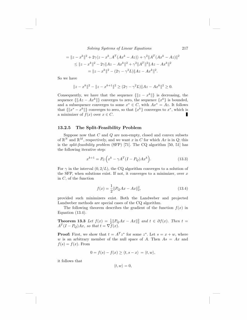
Solving Systems of Linear Equations 217
= ‖z − xk‖2 + 2γ〈z − xk, AT (Axk −Az)〉+ γ2‖AT (Axk −Az)‖2
≤ ‖z − xk‖2 − 2γ‖Az −Axk‖2 + γ2‖AT ‖2‖Az −Axk‖2
= ‖z − xk‖2 − (2γ − γ2L)‖Az −Axk‖2.
So we have
‖z − xk‖2 − ‖z − xk+1‖2 ≥ (2γ − γ2L)‖Az −Axk‖2 ≥ 0.
Consequently, we have that the sequence {‖z − xk‖} is decreasing, thesequence {‖Az − Axk‖} converges to zero, the sequence {xk} is bounded,and a subsequence converges to some x∗ ∈ C, with Ax∗ = Az. It followsthat {‖x∗ − xk‖} converges to zero, so that {xk} converges to x∗, which isa minimizer of f(x) over x ∈ C.
13.2.5 The Split-Feasibility Problem
Suppose now that C and Q are non-empty, closed and convex subsetsof RN and RM , respectively, and we want x in C for which Ax is in Q; thisis the split-feasibility problem (SFP) [71]. The CQ algorithm [50, 51] hasthe following iterative step:
xk+1 = PC
(xk − γAT (I − PQ)Axk
). (13.3)
For γ in the interval (0, 2/L), the CQ algorithm converges to a solution ofthe SFP, when solutions exist. If not, it converges to a minimizer, over xin C, of the function
f(x) =1
2‖PQAx−Ax‖22, (13.4)
provided such minimizers exist. Both the Landweber and projectedLandweber methods are special cases of the CQ algorithm.
The following theorem describes the gradient of the function f(x) inEquation (13.4).
Theorem 13.3 Let f(x) = 12‖PQAx − Ax‖22 and t ∈ ∂f(x). Then t =
AT (I − PQ)Ax, so that t = ∇f(x).
Proof: First, we show that t = AT z∗ for some z∗. Let s = x + w, wherew is an arbitrary member of the null space of A. Then As = Ax andf(s) = f(x). From
0 = f(s)− f(x) ≥ 〈t, s− x〉 = 〈t, w〉,
it follows that〈t, w〉 = 0,

218 A First Course in Optimization
for all w in the null space of A, from which we conclude that t is in therange of AT . Therefore, we can write t = AT z∗.
Let u be chosen so that ‖A(u− x)‖ = 1, and let ε > 0. We then have
‖PQAx−A(x+ ε(u− x))‖2 − ‖PQAx−Ax‖2 ≥
‖PQ(Ax+ ε(u− x))−A(x+ ε(u− x))‖2 − ‖PQAx−Ax‖2 ≥ 2ε〈t, u− x〉.
Therefore, since
‖PQAx−A(x+ε(u−x))‖2 = ‖PQAx−Ax‖2−2ε〈PQAx−Ax,A(u−x)〉+ε2,
it follows that
ε
2≥ 〈PQAx−Ax+ z∗, A(u− x)〉 = −〈AT (I − PQ)Ax− t, u− x〉.
Since ε is arbitrary, it follows that
〈AT (I − PQ)Ax− t, u− x〉 ≥ 0,
for all appropriate u. But this is also true if we replace u with v = 2x− u.Consequently, we have
〈AT (I − PQ)Ax− t, u− x〉 = 0.
Now we select
u− x = (AT (I − PQ)Ax− t)/‖AAT (I − PQ)Ax−At‖,
from which it follows that
AT (I − PQ)Ax = t.
Corollary 13.1 The gradient of the function
f(x) =1
2‖x− PCx‖2
is ∇f(x) = x− PCx, and the gradient of the function
g(x) =1
2
(‖x‖22 − ‖x− PCx‖22
)is ∇g(x) = PCx.
Extensions of the CQ algorithm have been applied recently to problemsin intensity-modulated radiation therapy [69, 73].
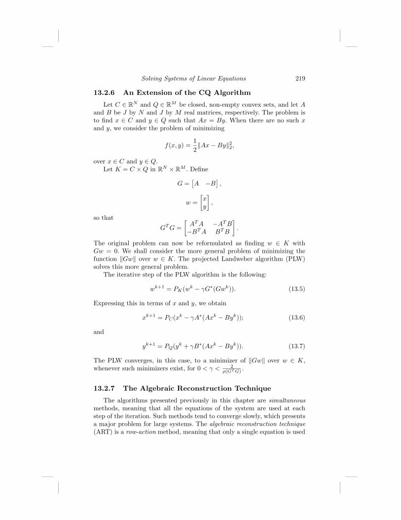
Solving Systems of Linear Equations 219
13.2.6 An Extension of the CQ Algorithm
Let C ∈ RN and Q ∈ RM be closed, non-empty convex sets, and let Aand B be J by N and J by M real matrices, respectively. The problem isto find x ∈ C and y ∈ Q such that Ax = By. When there are no such xand y, we consider the problem of minimizing
f(x, y) =1
2‖Ax−By‖22,
over x ∈ C and y ∈ Q.Let K = C ×Q in RN × RM . Define
G =[A −B
],
w =
[xy
],
so that
GTG =
[ATA −ATB−BTA BTB
].
The original problem can now be reformulated as finding w ∈ K withGw = 0. We shall consider the more general problem of minimizing thefunction ‖Gw‖ over w ∈ K. The projected Landweber algorithm (PLW)solves this more general problem.
The iterative step of the PLW algorithm is the following:
wk+1 = PK(wk − γG∗(Gwk)). (13.5)
Expressing this in terms of x and y, we obtain
xk+1 = PC(xk − γA∗(Axk −Byk)); (13.6)
and
yk+1 = PQ(yk + γB∗(Axk −Byk)). (13.7)
The PLW converges, in this case, to a minimizer of ‖Gw‖ over w ∈ K,whenever such minimizers exist, for 0 < γ < 2
ρ(GTG).
13.2.7 The Algebraic Reconstruction Technique
The algorithms presented previously in this chapter are simultaneousmethods, meaning that all the equations of the system are used at eachstep of the iteration. Such methods tend to converge slowly, which presentsa major problem for large systems. The algebraic reconstruction technique(ART) is a row-action method, meaning that only a single equation is used

220 A First Course in Optimization
at each step of the iteration. The ART has the following iterative step: fork = 0, 1, ... and m = k(modM) + 1, let
xk+1n = xkn +Amn(bm − (Axk)m)/
N∑j=1
|Amj |2. (13.8)
We can describe the ART geometrically as follows: once we have xk andm, the vector xk+1 is the orthogonal projection of xk onto the hyperplaneHm given by
Hm = {x|(Ax)m = bm}.
The Landweber algorithm can be similarly described: the vector xk+1 is aweighted sum of the orthogonal projections of xk onto each of the hyper-planes Hm, for all m.
In the consistent case, when the system Ax = b has solutions, the ARTconverges to the solution for which ‖x−x0‖ is minimized. Unlike the simul-taneous methods, when no solution exists, the ART sequence {xk} does notconverge to a single vector, but subsequences do converge to members of alimit cycle consisting of (typically) M distinct vectors. Generally speaking,the ART will converge, in the consistent case, faster than the Landwebermethod, especially if the equations are selected in a random order [127].
13.2.8 Double ART
Because the ART is significantly faster to converge than the Landwebermethod in the consistent case, we would like to be able to use the ART inthe inconsistent case, as well, to get a least-squares solution. To avoid thelimit-cycle behavior of ART in this case, we can use double ART (DART).
We know from basic linear algebra that the vector b can be written as
b = Ax+ w,
where xminimizes the function ‖b−Ax‖2 and w = w minimizes the function‖b − w‖2, subject to ATw = 0. Said another way, Ax is the orthogonalprojection of b onto the range of A and w is the orthogonal projection of bonto the null space of AT .
In DART we apply the ART algorithm twice, first to the consistentlinear system ATw = 0, with w0 = b, so that the limit is w, and then tothe consistent system Ax = b− w. The result is the minimizer of ‖b−Ax‖for which ‖x− x0‖ is minimized.

Solving Systems of Linear Equations 221
13.3 Regularization
In many applications in which systems of linear equations must besolved, the entries of the vector b are measured data and Ax = b is amodel that attempts to describe, in a somewhat simplified way, how b de-pends on the unknown vector x. The statistical noise in the measured dataintroduces one type of error, while the approximate nature of the modelitself introduces another. Because the model is simplified, but the data b isnoisy, an exact solution x itself usually ends up noisy. Also, it is commonfor the system to be ill-conditioned, that is, for small changes in b to leadto large changes in the exact solution x. This happens when the ratio ofthe largest to smallest eigenvalues of the matrix ATA is large. In such caseseven a minimum-norm solution of Ax = b can have a large norm. Conse-quently, we often do not want an exact solution of Ax = b, even when suchsolutions exist. Instead, we regularize the problem.
13.3.1 Norm-Constrained Least-Squares
One way to regularize the problem is to minimize not ‖b − Ax‖2, but,say,
f(x) = ‖b−Ax‖22 + ε2‖x‖22, (13.9)
for some small ε > 0. Now we are still trying to make ‖b−Ax‖2 small, butmanaging to keep ‖x‖2 from becoming too large in the process. This leadsto a norm-constrained least-squares solution.
The minimizer of f(x) is the unique solution xε of the system
(ATA+ ε2I)x = AT b. (13.10)
When M and N are large, we need ways to solve this system without havingto deal with the matrix ATA + ε2I. The Landweber method allowed usto avoid ATA in calculating the least-squares solution. Is there a similarmethod to use now? Yes, there is.
13.3.2 Regularizing Landweber’s Algorithm
Our goal is to minimize the function f(x) in Equation (13.9). Noticethat this is equivalent to minimizing the function
F (x) = ||Bx− c||22, (13.11)
for
B =
[AεI
], (13.12)

222 A First Course in Optimization
and
c =
[b0
], (13.13)
where 0 denotes a column vector with all entries equal to zero. The Landwe-ber iteration for the problem Bx = c is
xk+1 = xk + αBT (c−Bxk), (13.14)
for 0 < α < 2/ρ(BTB), where ρ(BTB) is the largest eigenvalue, or thespectral radius, of BTB. Equation (13.14) can be written as
xk+1 = (1− αε2)xk + αAT (b−Axk). (13.15)
13.3.3 Regularizing the ART
We would like to get the regularized solution xε by taking advantage ofthe faster convergence of the ART. Fortunately, there are ways to find xε,using only the matrix A and the ART algorithm. We discuss two methodsfor using ART to obtain regularized solutions of Ax = b. The first one ispresented in [53], while the second one is due to Eggermont, Herman, andLent [105].
In our first method we use ART to solve the system of equations givenin matrix form by [
AT εI] [uv
]= 0. (13.16)
We begin with u0 = b and v0 = 0. Then, the lower component of the limitvector is v∞ = −εxε, while the upper limit is u∞ = b−Axε.
The method of Eggermont et al. is similar. In their method we use ARTto solve the system of equations given in matrix form by[
A εI] [xv
]= b. (13.17)
We begin at x0 = 0 and v0 = 0. Then, the limit vector has for its uppercomponent x∞ = xε, and εv∞ = b−Axε.
13.4 Non-Negative Systems of Linear Equations
We turn now to non-negative systems of linear equations, which we shalldenote by y = Px, with the understanding that P is an I by J matrix with

Solving Systems of Linear Equations 223
non-negative entries Pij , such that, for each j, the column sum
sj =
I∑i=1
Pij
is positive, y is an I by 1 vector with positive entries yi, and we seek asolution x with non-negative entries xj . We say that the system is consistentwhenever such non-negative solutions exist. Denote by X the set of all non-negative x for which the vector Px has only positive entries. In what follows,all vectors x will lie in X and the initial vector x0 will always be positive.
13.4.1 The Multiplicative ART
Both the algebraic reconstruction technique (ART) and the multiplica-tive algebraic reconstruction technique (MART) were introduced by Gor-don, Bender and Herman [121] as two iterative methods for discrete imagereconstruction in transmission tomography. It was noticed somewhat laterthat the ART is a special case of Kaczmarz’s algorithm [134].
Both methods are what are called row-action methods, meaning thateach step of the iteration uses only a single equation from the system. TheMART is limited to non-negative systems for which non-negative solutionsare sought. In the under-determined case, both algorithms find the solutionclosest to the starting vector, in the two-norm or weighted two-norm sensefor ART, and in the cross-entropy sense for MART, so both algorithmscan be viewed as solving optimization problems. We consider two differentversions of the MART.
13.4.1.1 MART I
The iterative step of the first version of MART, which we call MARTI, is the following: for k = 0, 1, ..., and i = k(mod I) + 1, let
xk+1j = xkj
( yi(Pxk)i
)Pij/mi
,
for j = 1, ..., J , where the parameter mi is defined to be
mi = max{Pij |j = 1, ..., J}.
The MART I algorithm converges, in the consistent case, to the non-negative solution for which the KL distance KL(x, x0) is minimized.

224 A First Course in Optimization
13.4.1.2 MART II
The iterative step of the second version of MART, which we shall callMART II, is the following: for k = 0, 1, ..., and i = k(mod I) + 1, let
xk+1j = xkj
( yi(Pxk)i
)Pij/sjni
,
for j = 1, ..., J , where the parameter ni is defined to be
ni = max{Pijs−1j |j = 1, ..., J}.
The MART II algorithm converges, in the consistent case, to the non-negative solution for which the KL distance
J∑j=1
sjKL(xj , x0j )
is minimized. Just as the Landweber method is a simultaneous cousin ofthe row-action ART, there is a simultaneous cousin of the MART, called,not surprisingly, the simultaneous MART (SMART).
13.4.2 The Simultaneous MART
The SMART minimizes the cross-entropy, or Kullback-Leibler distance,f(x) = KL(Px, y), over nonnegative vectors x [93, 81, 184, 39].
Having found the vector xk, the next vector in the SMART sequence isxk+1, with entries given by
xk+1j = xkj exp
(s−1j
I∑i=1
Pij log( yi
(Pxk)i
)). (13.18)
As with MART II, when there are non-negative solutions of y = Px, theSMART converges to the solution for which the KL distance
J∑j=1
sjKL(xj , x0j )
is minimized.
13.4.3 The EMML Iteration
The expectation maximization maximum likelihood algorithm (EMML)minimizes the function f(x) = KL(y, Px), over nonnegative vectors x [186,

Solving Systems of Linear Equations 225
144, 199, 145, 39]. Having found the vector xk, the next vector in the EMMLsequence is xk+1, with entries given by
xk+1j = xkj s
−1j
( I∑i=1
Pij
( yi(Pxk)i
)). (13.19)
The iterative step of the EMML is closely related to that of the SMART,except that the exponentiation and logarithm are missing. When there arenon-negative solutions of the system y = Px, the EMML converges toa non-negative solution, but no further information about this solution isknown. Both the SMART and the EMML are slow to converge, particularlywhen the system is large.
13.4.4 Alternating Minimization
In [39] the SMART and the EMML were derived using the followingalternating minimization approach.
For each x ∈ X , let r(x) and q(x) be the I by J arrays with entries
r(x)ij = xjPijyi/(Px)i, (13.20)
and
q(x)ij = xjPij . (13.21)
In the iterative step of the SMART we get xk+1 by minimizing the function
KL(q(x), r(xk)) =
I∑i=1
J∑j=1
KL(q(x)ij , r(xk)ij)
over x ≥ 0. Note that KL(Px, y) = KL(q(x), r(x)). Similarly, the iterativestep of the EMML is to minimize the function KL(r(xk), q(x)) to get x =xk+1. Note that KL(y, Px) = KL(r(x), q(x)).
13.4.5 The Row-Action Variant of EMML
When there are non-negative solutions of y = Px, the MART con-verges faster than the SMART, and to the same solution. The SMARTinvolves exponentiation and a logarithm, and the MART a non-integralpower, both of which complicate their calculation. The EMML is consider-ably simpler in this respect, but, like SMART, converges slowly. We wouldlike to have a row-action variant of the EMML that converges faster thanthe EMML in the consistent case, but is easier to calculate than the MART.The EM-MART is such an algorithm. As with the MART, we distinguish

226 A First Course in Optimization
two versions, EM-MART I and EM-MART II. When the system y = Pxhas non-negative solutions, both EM-MART I and EM-MART II convergeto non-negative solutions, but nothing further is known about these solu-tions. To motivate these algorithms, we rewrite the MART algorithms asfollows:
13.4.5.1 MART I
The iterative step of MART I can be written as follows: for k = 0, 1, ...,and i = k(mod I) + 1, let
xk+1j = xkj exp
((Pijmi
)log( yi
(Pxk)i
)),
or, equivalently, as
log xk+1j =
(1− Pij
mi
)log xkj +
(Pijmi
)log(xkj
yi(Pxk)i
). (13.22)
13.4.5.2 MART II
Similarly, the iterative step of MART II can be written as follows: fork = 0, 1, ..., and i = k(mod I) + 1, let
xk+1j = xkj exp
(( Pijsjni
)log( yi
(Pxk)i
)),
or, equivalently, as
log xk+1j =
(1− Pij
sjni
)log xkj +
( Pijsjni
)log(xkj
yi(Pxk)i
). (13.23)
We obtain the EM-MART I and EM-MART II simply by removing thelogarithms in Equations (13.22) and (13.23), respectively.
13.4.5.3 EM-MART I
The iterative step of EM-MART I is as follows: for k = 0, 1, ..., andi = k(mod I) + 1, let
xk+1j =
(1− Pij
mi
)xkj +
(Pijmi
)(xkj
yi(Pxk)i
). (13.24)
13.4.5.4 EM-MART II
The iterative step of EM-MART II is as follows:
xk+1j =
(1− Pij
sjni
)xkj +
( Pijsjni
)(xkj
yi(Pxk)i
). (13.25)

Solving Systems of Linear Equations 227
13.5 Regularized SMART and EMML
As with the Landweber algorithm, there are situations that arise inpractice in which, because of noisy measurements, the exact or approximatesolutions of y = Px provided by the SMART and EMML algorithms arenot suitable. In such cases, we need to regularize the SMART and theEMML, which is usually done by including a penalty function.
13.5.1 Regularized SMART
As we have seen, the iterative step of the SMART is obtained by mini-mizing the function KL(q(x), r(xk)) over non-negative x, and the limit ofthe SMART minimizes KL(Px, y). We can regularize by minimizing
KL(Px, y) +KL(x, p),
where the vector p with positive entries pj is a prior estimate of the solution.To obtain xk+1 from xk, we minimize
KL(q(x), r(xk)) +
J∑j=1
δjKL(xj , pj).
There are many penalty functions we could use here, but the one we havechosen permits the minimizing xk+1 to be obtained in closed form.
The iterative step of the regularized SMART is as follows:
log xk+1j =
δjδj + sj
log pj +1
δj + sjxkj
I∑i=1
Pij log( yi
(Pxk)i
). (13.26)
13.5.2 Regularized EMML
As we have seen, the iterative step of the EMML is obtained by mini-mizing the function KL(r(xk), q(x)) over non-negative x, and the limit ofthe EMML minimizes KL(y, Px). We can regularize by minimizing
KL(y, Px) +KL(p, x).
To obtain xk+1 from xk, we minimize
KL(r(xk), q(x)) +
J∑j=1
δjKL(pj , xj).
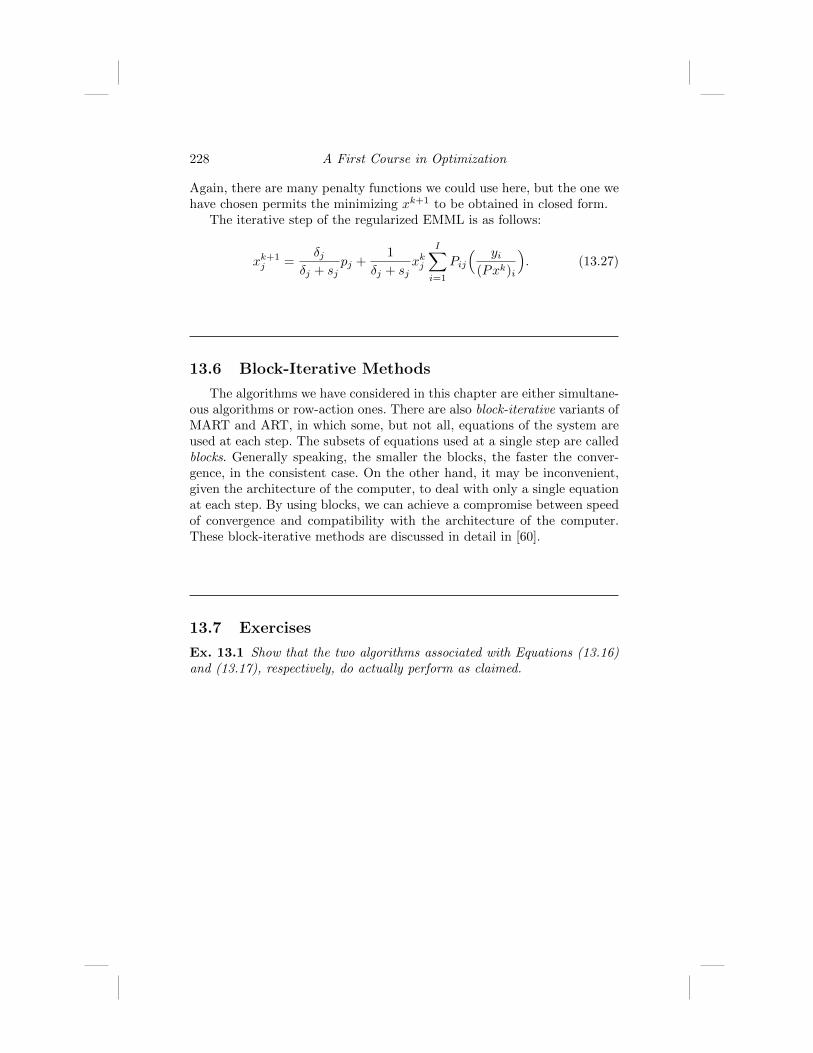
228 A First Course in Optimization
Again, there are many penalty functions we could use here, but the one wehave chosen permits the minimizing xk+1 to be obtained in closed form.
The iterative step of the regularized EMML is as follows:
xk+1j =
δjδj + sj
pj +1
δj + sjxkj
I∑i=1
Pij
( yi(Pxk)i
). (13.27)
13.6 Block-Iterative Methods
The algorithms we have considered in this chapter are either simultane-ous algorithms or row-action ones. There are also block-iterative variants ofMART and ART, in which some, but not all, equations of the system areused at each step. The subsets of equations used at a single step are calledblocks. Generally speaking, the smaller the blocks, the faster the conver-gence, in the consistent case. On the other hand, it may be inconvenient,given the architecture of the computer, to deal with only a single equationat each step. By using blocks, we can achieve a compromise between speedof convergence and compatibility with the architecture of the computer.These block-iterative methods are discussed in detail in [60].
13.7 Exercises
Ex. 13.1 Show that the two algorithms associated with Equations (13.16)and (13.17), respectively, do actually perform as claimed.

Chapter 14
Conjugate-Direction Methods
14.1 Chapter Summary . . . . . . . . . . . . . . . . . . . . . . . . . . . . . . . . . . . . . . . . . . . . . . . 22914.2 Iterative Minimization . . . . . . . . . . . . . . . . . . . . . . . . . . . . . . . . . . . . . . . . . . . 22914.3 Quadratic Optimization . . . . . . . . . . . . . . . . . . . . . . . . . . . . . . . . . . . . . . . . . . 23014.4 Conjugate Bases for RJ . . . . . . . . . . . . . . . . . . . . . . . . . . . . . . . . . . . . . . . . . . 233
14.4.1 Conjugate Directions . . . . . . . . . . . . . . . . . . . . . . . . . . . . . . . . . . . . 23314.4.2 The Gram-Schmidt Method . . . . . . . . . . . . . . . . . . . . . . . . . . . . . 234
14.5 The Conjugate Gradient Method . . . . . . . . . . . . . . . . . . . . . . . . . . . . . . . . 23514.5.1 The Main Idea . . . . . . . . . . . . . . . . . . . . . . . . . . . . . . . . . . . . . . . . . . . 23514.5.2 A Recursive Formula . . . . . . . . . . . . . . . . . . . . . . . . . . . . . . . . . . . . 236
14.6 Krylov Subspaces . . . . . . . . . . . . . . . . . . . . . . . . . . . . . . . . . . . . . . . . . . . . . . . . 23714.7 Extensions of the CGM . . . . . . . . . . . . . . . . . . . . . . . . . . . . . . . . . . . . . . . . . . 23714.8 Exercises . . . . . . . . . . . . . . . . . . . . . . . . . . . . . . . . . . . . . . . . . . . . . . . . . . . . . . . . . 237
14.1 Chapter Summary
Finding the least-squares solution of a possibly inconsistent system oflinear equations Ax = b is equivalent to minimizing the quadratic functionf(x) = 1
2 ||Ax − b||22 and so can be viewed within the framework of opti-
mization. Iterative optimization methods can then be used to provide, orat least suggest, algorithms for obtaining the least-squares solution. Theconjugate gradient method is one such method. Proofs for the lemmas inthis chapter are exercises for the reader.
14.2 Iterative Minimization
Iterative methods for minimizing a real-valued function f(x) over thevector variable x usually take the following form: having obtained xk−1,a new direction vector dk is selected, an appropriate scalar αk > 0 is
229

230 A First Course in Optimization
determined and the next member of the iterative sequence is given by
xk = xk−1 + αkdk. (14.1)
Ideally, one would choose the αk to be the value of α for which the functionf(xk−1 +αdk) is minimized. It is assumed that the direction dk is a descentdirection; that is, for small positive α the function f(xk−1 +αdk) is strictlydecreasing. Finding the optimal value of α at each step of the iteration isdifficult, if not impossible, in most cases, and approximate methods, usingline searches, are commonly used.
Lemma 14.1 When xk is constructed using the optimal α, we have
∇f(xk) · dk = 0. (14.2)
Proof: Differentiate the function f(xk−1+αdk) with respect to the variableα.
Since the gradient ∇f(xk) is orthogonal to the previous direction vectordk and also because −∇f(x) is the direction of greatest decrease of f(x),the choice of dk+1 = −∇f(xk) as the next direction vector is a reasonableone. With this choice we obtain Cauchy’s steepest descent method [150]:
xk+1 = xk − αk+1∇f(xk).
The steepest descent method need not converge in general and even whenit does, it can do so slowly, suggesting that there may be better choicesfor the direction vectors. For example, the Newton-Raphson method [163]employs the following iteration:
xk+1 = xk −∇2f(xk)−1∇f(xk),
where ∇2f(x) is the Hessian matrix for f(x) at x. To investigate furtherthe issues associated with the selection of the direction vectors, we considerthe more tractable special case of quadratic optimization.
14.3 Quadratic Optimization
Let A be an arbitrary real I by J matrix. The linear system of equationsAx = b need not have any solutions, and we may wish to find a least-squaressolution x = x that minimizes
f(x) =1
2||b−Ax||22. (14.3)

Conjugate-Direction Methods 231
The vector b can be written
b = Ax+ w,
where AT w = 0 and a least squares solution is an exact solution of thelinear system Qx = c, with Q = ATA and c = AT b. We shall assumethat Q is invertible and there is a unique least squares solution; this is thetypical case.
We consider now the iterative scheme described by Equation (14.1) forf(x) as in Equation (14.3). For now, the direction vectors dk are arbitrary.For this f(x) the gradient becomes
∇f(x) = Qx− c.
The optimal αk for the iteration can be obtained in closed form.
Lemma 14.2 The optimal αk is
αk =rk · dk
dk ·Qdk, (14.4)
where rk = c−Qxk−1.
Lemma 14.3 Let ||x||2Q = x · Qx denote the square of the Q-norm of x.Then
||x− xk−1||2Q − ||x− xk||2Q = (rk · dk)2/dk ·Qdk ≥ 0
for any direction vectors dk.
If the sequence of direction vectors {dk} is completely general, the iter-ative sequence need not converge. However, if the set of direction vectorsis finite and spans RJ and we employ them cyclically, convergence follows.
Theorem 14.1 Let {d1, ..., dJ} be any basis for RJ . Let αk be chosen ac-cording to Equation (14.4). Then, for k = 1, 2, ..., j = k(mod J), and anyx0, the sequence defined by
xk = xk−1 + αkdj
converges to the least squares solution.
Proof: The sequence {||x−xk||2Q} is decreasing and, therefore, the sequence
{(rk · dk)2/dk · Qdk must converge to zero. Therefore, the vectors xk arebounded, and for each j = 1, ..., J , the subsequences {xmJ+j , m = 0, 1, ...}have cluster points, say x∗,j with
x∗,j = x∗,j−1 +(c−Qx∗,j−1) · dj
dj ·Qdjdj .

232 A First Course in Optimization
SincermJ+j · dj → 0,
it follows that, for each j = 1, ..., J ,
(c−Qx∗,j) · dj = 0.
Therefore,x∗,1 = ... = x∗,J = x∗
with Qx∗ = c. Consequently, x∗ is the least squares solution and the se-quence {||x∗ − xk||Q} is decreasing. But a subsequence converges to zero;therefore, {||x∗ − xk||Q} → 0. This completes the proof.
There is an interesting corollary to this theorem that pertains to amodified version of the ART algorithm. For k = 0, 1, ... and i = k(modM)+1 and with the rows of A normalized to have length one, the ART iterativestep is
xk+1 = xk + (bi − (Axk)i)ai,
where ai is the ith column of AT . When Ax = b has no solutions, theART algorithm does not converge to the least-squares solution; rather,it exhibits subsequential convergence to a limit cycle. However, using theprevious theorem, we can show that the following modification of the ART,which we shall call the least squares ART (LS-ART), converges to the least-squares solution for every x0:
xk+1 = xk +rk+1 · ai
ai ·Qaiai.
In the quadratic case the steepest descent iteration has the form
xk = xk−1 +rk · rk
rk ·Qrkrk.
We have the following result.
Theorem 14.2 The steepest descent method converges to the least-squaressolution.
Proof: As in the proof of the previous theorem, we have
||x− xk−1||2Q − ||x− xk||2Q = (rk · dk)2/dk ·Qdk ≥ 0,
where now the direction vectors are dk = rk. So, the sequence {||x−xk||2Q}is decreasing, and therefore the sequence {(rk ·rk)2/rk ·Qrk} must convergeto zero. The sequence {xk} is bounded; let x∗ be a cluster point. It followsthat c−Qx∗ = 0, so that x∗ is the least-squares solution x. The rest of theproof follows as in the proof of the previous theorem.
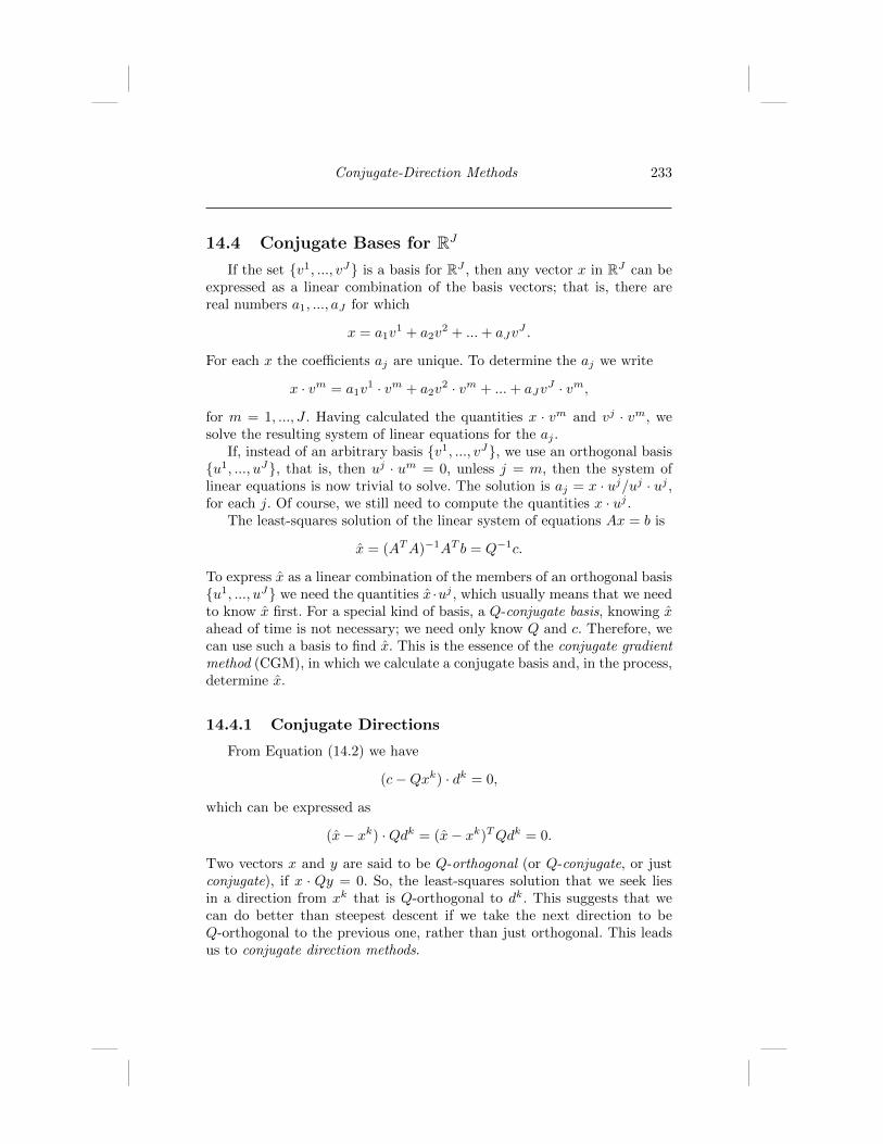
Conjugate-Direction Methods 233
14.4 Conjugate Bases for RJ
If the set {v1, ..., vJ} is a basis for RJ , then any vector x in RJ can beexpressed as a linear combination of the basis vectors; that is, there arereal numbers a1, ..., aJ for which
x = a1v1 + a2v
2 + ...+ aJvJ .
For each x the coefficients aj are unique. To determine the aj we write
x · vm = a1v1 · vm + a2v
2 · vm + ...+ aJvJ · vm,
for m = 1, ..., J . Having calculated the quantities x · vm and vj · vm, wesolve the resulting system of linear equations for the aj .
If, instead of an arbitrary basis {v1, ..., vJ}, we use an orthogonal basis{u1, ..., uJ}, that is, then uj · um = 0, unless j = m, then the system oflinear equations is now trivial to solve. The solution is aj = x · uj/uj · uj ,for each j. Of course, we still need to compute the quantities x · uj .
The least-squares solution of the linear system of equations Ax = b is
x = (ATA)−1AT b = Q−1c.
To express x as a linear combination of the members of an orthogonal basis{u1, ..., uJ} we need the quantities x ·uj , which usually means that we needto know x first. For a special kind of basis, a Q-conjugate basis, knowing xahead of time is not necessary; we need only know Q and c. Therefore, wecan use such a basis to find x. This is the essence of the conjugate gradientmethod (CGM), in which we calculate a conjugate basis and, in the process,determine x.
14.4.1 Conjugate Directions
From Equation (14.2) we have
(c−Qxk) · dk = 0,
which can be expressed as
(x− xk) ·Qdk = (x− xk)TQdk = 0.
Two vectors x and y are said to be Q-orthogonal (or Q-conjugate, or justconjugate), if x · Qy = 0. So, the least-squares solution that we seek liesin a direction from xk that is Q-orthogonal to dk. This suggests that wecan do better than steepest descent if we take the next direction to beQ-orthogonal to the previous one, rather than just orthogonal. This leadsus to conjugate direction methods.

234 A First Course in Optimization
Definition 14.1 We say that the set {p1, ..., pn} is a conjugate set for RJif pi ·Qpj = 0 for i 6= j.
Lemma 14.4 A conjugate set that does not contain zero is linearly inde-pendent. If pn 6= 0 for n = 1, ..., J , then the least-squares vector x can bewritten as
x = a1p1 + ...+ aJp
J ,
with aj = c · pj/pj ·Qpj for each j.
Proof: Use the Q-inner product 〈x, y〉Q = x ·Qy.
Therefore, once we have a conjugate basis, computing the least squaressolution is trivial. Generating a conjugate basis can obviously be done usingthe standard Gram-Schmidt approach.
14.4.2 The Gram-Schmidt Method
Let {v1, ..., vJ} be a linearly independent set of vectors in the spaceRM , where J ≤ M . The Gram-Schmidt method uses the vj to create anorthogonal basis {u1, ..., uJ} for the span of the vj . Begin by taking u1 = v1.For j = 2, ..., J , let
uj = vj − u1 · vj
u1 · u1u1 − ...− uj−1 · vj
uj−1 · uj−1uj−1.
To apply this approach to obtain a conjugate basis, we would simply replacethe dot products uk · vj and uk · uk with the Q-inner products, that is,
pj = vj − p1 ·Qvj
p1 ·Qp1p1 − ...− pj−1 ·Qvj
pj−1 ·Qpj−1pj−1. (14.5)
Even though the Q-inner products can always be written as x · Qy =Ax ·Ay, so that we need not compute the matrix Q, calculating a conjugatebasis using Gram-Schmidt is not practical for large J . There is a way out,fortunately.
If we take p1 = v1 and vj = Qpj−1, we have a much more efficientmechanism for generating a conjugate basis, namely a three-term recursionformula [150]. The set {p1, Qp1, ..., QpJ−1} need not be a linearly indepen-dent set, in general, but, if our goal is to find x, and not really to calculatea full conjugate basis, this does not matter, as we shall see.
Theorem 14.3 Let p1 6= 0 be arbitrary. Let p2 be given by
p2 = Qp1 − Qp1 ·Qp1
p1 ·Qp1p1,

Conjugate-Direction Methods 235
so that p2 ·Qp1 = 0. Then, for n ≥ 2, let pn+1 be given by
pn+1 = Qpn − Qpn ·Qpn
pn ·Qpnpn − Qpn−1 ·Qpn
pn−1 ·Qpn−1pn−1. (14.6)
Then, the set {p1, ..., pJ} is a conjugate set for RJ . If pn 6= 0 for each n,then the set is a conjugate basis for RJ .
Proof: We consider the induction step of the proof. Assume that{p1, ..., pn} is aQ-orthogonal set of vectors; we then show that {p1, ..., pn+1}is also, provided that n ≤ J − 1. It is clear from Equation (14.6) that
pn+1 ·Qpn = pn+1 ·Qpn−1 = 0.
For j ≤ n− 2, we have
pn+1 ·Qpj = pj ·Qpn+1 = pj ·Q2pn − apj ·Qpn − bpj ·Qpn−1,
for constants a and b. The second and third terms on the right side arethen zero because of the induction hypothesis. The first term is also zerosince
pj ·Q2pn = (Qpj) ·Qpn = 0
because Qpj is in the span of {p1, ..., pj+1}, and so is Q-orthogonal to pn.
The calculations in the three-term recursion formula Equation (14.6)also occur in the Gram-Schmidt approach in Equation (14.5); the point isthat Equation (14.6) uses only the first three terms, in every case.
14.5 The Conjugate Gradient Method
14.5.1 The Main Idea
The main idea in the conjugate gradient method (CGM) is to build theconjugate set as we calculate the least squares solution using the iterativealgorithm
xn = xn−1 + αnpn. (14.7)
The αn is chosen so as to minimize f(xn−1 + αpn), as a function of α. Sowe have
αn =rn · pn
pn ·Qpn,

236 A First Course in Optimization
where rn = c − Qxn−1. Since the function f(x) = 12 ||Ax − b||22 has for
its gradient ∇f(x) = AT (Ax − b) = Qx − c, the residual vector rn =c − Qxn−1 is the direction of steepest descent from the point x = xn−1.The CGM combines the use of the negative gradient directions from thesteepest descent method with the use of a conjugate basis of directions, byusing the rn+1 to construct the next direction pn+1 in such a way as toform a conjugate set {p1, ..., pJ}.
14.5.2 A Recursive Formula
As before, there is an efficient recursive formula that provides the nextdirection: let p1 = r1 = (c−Qx0) and for j = 2, 3, ...
pj = rj − βj−1pj−1, (14.8)
with
βj−1 =rj ·Qpj−1
pj−1 ·Qpj−1. (14.9)
Note that it follows from the definition of βj−1 that
pjQpj−1 = 0. (14.10)
Since the αn is the optimal choice and
rn+1 = −∇f(xn),
we have, according to Equation (14.2),
rn+1 · pn = 0. (14.11)
In theory, the CGM converges to the least squares solution in finitelymany steps, since we either reach pn+1 = 0 or n + 1 = J . In practice, theCGM can be employed as a fully iterative method by cycling back throughthe previously used directions.
An induction proof similar to the one used to prove Theorem 14.3 es-tablishes that the set {p1, ..., pJ} is a conjugate set [150, 163]. In fact, wecan say more.
Theorem 14.4 For n = 1, 2, ..., J and j = 1, ..., n− 1 we have
• a) rn · rj = 0;
• b) rn · pj = 0; and
• c) pn ·Qpj = 0.
The proof presented here through a series of exercises at the end of thechapter is based on that given in [163].

Conjugate-Direction Methods 237
14.6 Krylov Subspaces
Another approach to deriving the conjugate gradient method is to useKrylov subspaces. If we select x0 = 0 as our starting vector for the CGM,then p1 = r1 = c, and each pn+1 and xn+1 lie in the Krylov subspaceKn(Q, c), defined to be the span of the vectors {c,Qc,Q2c, ..., Qnc}.
For any x in RJ , we have
‖x− x‖2Q = (x− x)TQ(x− x).
Minimizing ‖x− x‖2Q over all x in Kn(Q, c) is equivalent to minimizing the
same function over all x of the form x = xn + αpn+1. This, in turn, isequivalent to minimizing
−2αpn+1 · rn+1 + α2pn+1 ·Qpn+1,
over all α, which has for its solution the value α = αn+1 used to calculatexn+1 in the CGM.
14.7 Extensions of the CGM
The convergence rate of the CGM depends on the condition number ofthe matrix Q, which is the ratio of its largest to its smallest eigenvalues.When the condition number is much greater than one convergence can beaccelerated by preconditioning the matrix Q; this means replacing Q withP−1/2QP−1/2, for some positive-definite approximation P of Q (see [7]).
There are versions of the CGM for the minimization of non-quadraticfunctions. In the quadratic case the next conjugate direction pn+1 is builtfrom the residual rn+1 and pn. Since, in that case, rn+1 = −∇f(xn), thissuggests that in the non-quadratic case we build pn+1 from −∇f(xn) andpn. This leads to the Fletcher-Reeves method. Other similar algorithms,such as the Polak-Ribiere and the Hestenes-Stiefel methods, perform betteron certain problems [163].
14.8 Exercises
Ex. 14.1 There are several lemmas in this chapter whose proofs are onlysketched. Complete the proofs of these lemma.

238 A First Course in Optimization
The following exercises refer to the Conjugate Gradient Method.
Ex. 14.2 Show that
rn+1 = rn − αnQpn, (14.12)
so Qpn is in the span of rn+1 and rn.
Ex. 14.3 Prove that rn = 0 whenever pn = 0, in which case we havec = Qxn−1, so that xn−1 is the least-squares solution.
Ex. 14.4 Show that rn · pn = rn · rn, so that
αn =rn · rn
pn ·Qpn. (14.13)
The proof of Theorem 14.4 uses induction on the number n. Throughoutthe following exercises assume that the statements in Theorem 14.4 holdfor some fixed n with 2 ≤ n < J and for j = 1, 2, ..., n− 1. We prove thatthey hold also for n+ 1 and j = 1, 2, ..., n.
Ex. 14.5 Show that pn ·Qpn = rn ·Qpn, so that
αn =rn · rn
rn ·Qpn. (14.14)
Hints: use Equation (14.8) and the induction assumption concerning c) ofthe Theorem.
Ex. 14.6 Show that rn+1·rn = 0. Hint: use Equations (14.14) and (14.12).
Ex. 14.7 Show that rn+1 · rj = 0, for j = 1, ..., n − 1. Hints: write outrn+1 using Equation (14.12) and rj using Equation (14.8), and use theinduction hypotheses.
Ex. 14.8 Show that rn+1 · pj = 0, for j = 1, ..., n. Hints: use Equations(14.12) and (14.8) and induction assumptions b) and c).
Ex. 14.9 Show that pn+1 ·Qpj = 0, for j = 1, ..., n−1. Hints: use Equation(14.12), the previous exercise, and the induction assumptions.
The final step in the proof is to show that pn+1 · Qpn = 0. But thisfollows immediately from Equation (14.10).

Chapter 15
Operators
15.1 Chapter Summary . . . . . . . . . . . . . . . . . . . . . . . . . . . . . . . . . . . . . . . . . . . . . . . 24015.2 Operators . . . . . . . . . . . . . . . . . . . . . . . . . . . . . . . . . . . . . . . . . . . . . . . . . . . . . . . . . 24015.3 Contraction Operators . . . . . . . . . . . . . . . . . . . . . . . . . . . . . . . . . . . . . . . . . . . 240
15.3.1 Lipschitz Continuous Operators . . . . . . . . . . . . . . . . . . . . . . . . . 24115.3.2 Non-Expansive Operators . . . . . . . . . . . . . . . . . . . . . . . . . . . . . . . 24115.3.3 Strict Contractions . . . . . . . . . . . . . . . . . . . . . . . . . . . . . . . . . . . . . . 242
15.3.3.1 The Banach-Picard Theorem: . . . . . . . . . . . . . 24315.3.4 Eventual Strict Contractions . . . . . . . . . . . . . . . . . . . . . . . . . . . . 24315.3.5 Instability . . . . . . . . . . . . . . . . . . . . . . . . . . . . . . . . . . . . . . . . . . . . . . . . 244
15.4 Orthogonal Projection Operators . . . . . . . . . . . . . . . . . . . . . . . . . . . . . . . . 24415.4.1 Properties of the Operator PC . . . . . . . . . . . . . . . . . . . . . . . . . . 245
15.4.1.1 PC is Non-expansive . . . . . . . . . . . . . . . . . . . . . . . 24515.4.1.2 PC is Firmly Non-expansive . . . . . . . . . . . . . . . 24515.4.1.3 The Search for Other Properties of PC . . . . 246
15.5 Two Useful Identities . . . . . . . . . . . . . . . . . . . . . . . . . . . . . . . . . . . . . . . . . . . . 24615.6 Averaged Operators . . . . . . . . . . . . . . . . . . . . . . . . . . . . . . . . . . . . . . . . . . . . . . 24715.7 Gradient Operators . . . . . . . . . . . . . . . . . . . . . . . . . . . . . . . . . . . . . . . . . . . . . . 249
15.7.1 The Krasnosel’skii-Mann-Opial Theorem . . . . . . . . . . . . . . . 25015.8 Affine Linear Operators . . . . . . . . . . . . . . . . . . . . . . . . . . . . . . . . . . . . . . . . . . 251
15.8.1 The Hermitian Case . . . . . . . . . . . . . . . . . . . . . . . . . . . . . . . . . . . . . 25115.9 Paracontractive Operators . . . . . . . . . . . . . . . . . . . . . . . . . . . . . . . . . . . . . . . 252
15.9.1 Linear and Affine Paracontractions . . . . . . . . . . . . . . . . . . . . . 25215.9.2 The Elsner-Koltracht-Neumann Theorem . . . . . . . . . . . . . . . 254
15.10 Matrix Norms . . . . . . . . . . . . . . . . . . . . . . . . . . . . . . . . . . . . . . . . . . . . . . . . . . . . 25515.10.1 Induced Matrix Norms . . . . . . . . . . . . . . . . . . . . . . . . . . . . . . . . . . 25515.10.2 Condition Number of a Square Matrix . . . . . . . . . . . . . . . . . . 25615.10.3 Some Examples of Induced Matrix Norms . . . . . . . . . . . . . . 25715.10.4 The Euclidean Norm of a Square Matrix . . . . . . . . . . . . . . . 258
15.11 Exercises . . . . . . . . . . . . . . . . . . . . . . . . . . . . . . . . . . . . . . . . . . . . . . . . . . . . . . . . . 260
239
240 A First Course in Optimization
15.1 Chapter Summary
In a broad sense, all iterative algorithms generate a sequence {xk} ofvectors. The sequence may converge for any starting vector x0, or mayconverge only if the x0 is sufficiently close to a solution. The limit, when itexists, may depend on x0, and may, or may not, solve the original problem.Convergence to the limit may be slow and the algorithm may need to beaccelerated. The algorithm may involve measured data. The limit may besensitive to noise in the data and the algorithm may need to be regularizedto lessen this sensitivity. The algorithm may be quite general, applying toall problems in a broad class, or it may be tailored to the problem at hand.Each step of the algorithm may be costly, but only a few steps generallyneeded to produce a suitable approximate answer, or, each step may beeasily performed, but many such steps needed. Although convergence of analgorithm is important, theoretically, sometimes in practice only a few iter-ative steps are used. In this chapter we consider several classes of operatorsthat play important roles in optimization.
15.2 Operators
For most of the iterative algorithms we shall consider, the iterative stepis
xk+1 = Txk, (15.1)
for some operator T . If T is a continuous operator (and it usually is), andthe sequence {T kx0} converges to x, then T x = x, that is, x is a fixed pointof the operator T . We denote by Fix(T ) the set of fixed points of T . Theconvergence of the iterative sequence {T kx0} will depend on the propertiesof the operator T .
Our approach here will be to identify several classes of operators forwhich the iterative sequence is known to converge, to examine the conver-gence theorems that apply to each class, to describe several applied prob-lems that can be solved by iterative means, to present iterative algorithmsfor solving these problems, and to establish that the operator involved ineach of these algorithms is a member of one of the designated classes.
Operators 241
15.3 Contraction Operators
Contraction operators are perhaps the best known class of operatorsassociated with iterative algorithms.
15.3.1 Lipschitz Continuous Operators
Definition 15.1 An operator T on RJ is Lipschitz continuous, with re-spect to a vector norm || · ||, or L-Lipschitz, if there is a positive constantL such that
||Tx− Ty|| ≤ L||x− y||, (15.2)
for all x and y in RJ .
For example, if f : R→ R, and g(x) = f ′(x) is differentiable, the MeanValue Theorem tells us that
g(b) = g(a) + g′(c)(b− a),
for some c between a and b. Therefore,
|f ′(b)− f ′(a)| ≤ |f ′′(c)||b− a|.
If |f ′′(x)| ≤ L, for all x, then g(x) = f ′(x) is L-Lipschitz. More generally, iff : RJ → R is twice differentiable and ‖∇2f(x)‖2 ≤ L, for all x, then T =∇f is L-Lipschitz, with respect to the 2-norm. The 2-norm of the Hessianmatrix ∇2f(x) is the largest of the absolute values of its eigenvalues.
15.3.2 Non-Expansive Operators
An important special class of Lipschitz continuous operators are thenon-expansive, or contractive, operators.
Definition 15.2 If L = 1, then T is said to be non-expansive (ne), or acontraction, with respect to the given norm. In other words, T is ne for agiven norm if, for every x and y, we have
‖Tx− Ty‖ ≤ ‖x− y‖.
Lemma 15.1 Let T : RJ → RJ be a non-expansive operator, with respectto the 2-norm. Then the set F of fixed points of T is a convex set.

242 A First Course in Optimization
Proof: Select two distinct points a and b in F , a scalar α in the openinterval (0, 1), and let c = αa+ (1− α)b. We show that Tc = c. Note that
a− c =1− αα
(c− b).
We have
‖a−b‖ = ‖a−Tc+Tc−b‖ ≤ ‖a−Tc‖+‖Tc−b‖ = ‖Ta−Tc‖+‖Tc−Tb‖
≤ ‖a− c‖+ ‖c− b‖ = ‖a− b‖;
the last equality follows since a − c is a multiple of (c − b). From this, weconclude that
‖a− Tc‖ = ‖a− c‖,
‖Tc− b‖ = ‖c− b‖,
and that a − Tc and Tc− b are positive multiples of one another, that is,there is β > 0 such that
a− Tc = β(Tc− b),
or
Tc =1
1 + βa+
β
1 + βb = γa+ (1− γ)b.
Then inserting c = αa+ (1− α)b and Tc = γa+ (1− γ)b into
‖Tc− b‖ = ‖c− b‖,
we find that γ = α and so Tc = c.
The reader should note that the proof of the previous lemma dependsheavily on the fact that the norm is the two-norm. If x and y are any non-negative vectors then ‖x+ y‖1 = ‖x‖1 + ‖y‖1, so the proof would not hold,if, for example, we used the one-norm instead.
We want to find properties of an operator T that guarantee that thesequence of iterates {T kx0} will converge to a fixed point of T , for any x0,whenever fixed points exist. Being non-expansive is not enough; the non-expansive operator T = −I, where Ix = x is the identity operator, has thefixed point x = 0, but the sequence {T kx0} converges only if x0 = 0.
15.3.3 Strict Contractions
One property that guarantees not only that the iterates converge, butthat there is a fixed point is the property of being a strict contraction.

Operators 243
Definition 15.3 An operator T on RJ is a strict contraction (sc), withrespect to a vector norm || · ||, if there is r ∈ (0, 1) such that
||Tx− Ty|| ≤ r||x− y||, (15.3)
for all vectors x and y.
For strict contractions, we have the Banach-Picard Theorem [103].
15.3.3.1 The Banach-Picard Theorem:
Theorem 15.1 Let T be sc. Then, there is a unique fixed point of T and,for any starting vector x0, the sequence {T kx0} converges to the fixed point.
The key step in the proof is to show that {xk} is a Cauchy sequence,therefore, it has a limit.
Corollary 15.1 If Tn is a strict contraction, for some positive integer n,then T has a fixed point.
Proof: Suppose that Tnx = x. Then
TnT x = TTnx = T x,
so that both x and T x are fixed points of Tn. But Tn has a unique fixedpoint. Therefore, T x = x.
In many of the applications of interest to us, there will be multiplefixed points of T . Therefore, T will not be sc for any vector norm, andthe Banach-Picard fixed-point theorem will not apply. We need to considerother classes of operators. These classes of operators will emerge as weinvestigate the properties of orthogonal projection operators.
15.3.4 Eventual Strict Contractions
Consider the problem of finding x such that x = e−x. We can see fromthe graphs of y = x and y = e−x that there is a unique solution, which weshall denote by z. It turns out that z = 0.56714329040978.... Let us try tofind z using the iterative sequence xk+1 = e−xk , starting with some realx0. Note that we always have xk > 0 for k = 1, 2, ..., even if x0 < 0. Theoperator here is Tx = e−x, which, for simplicity, we view as an operatoron the non-negative real numbers.
Since the derivative of the function f(x) = e−x is f ′(x) = −e−x, wehave |f ′(x)| ≤ 1, for all non-negative x, so T is non-expansive. But we donot have |f ′(x)| ≤ r < 1, for all non-negative x; therefore, T is a not astrict contraction, when considered as an operator on the non-negative realnumbers.

244 A First Course in Optimization
If we choose x0 = 0, then x1 = 1, x2 = 0.368, approximately, and so on.Continuing this iteration a few more times, we find that after about k = 14,the value of xk settles down to 0.567, which is the answer, to three decimalplaces. The same thing is seen to happen for any positive starting points x0.It would seem that T has another property, besides being non-expansive,that is forcing convergence. What is it?
From the fact that 1− e−x ≤ x, for all real x, with equality if and onlyif x = 0, we can show easily that, for r = max{e−x1 , e−x2},
|z − xk+1| ≤ r|z − xk|,
for k = 3, 4, .... Since r < 1, it follows, just as in the proof of the Banach-Picard Theorem, that {xk} is a Cauchy sequence and therefore converges.The limit must be a fixed point of T , so the limit must be z.
Although the operator T is not a strict contraction, with respect to thenon-negative numbers, once we begin to calculate the sequence of iteratesthe operator T effectively becomes a strict contraction, with respect to thevectors of the particular sequence being constructed, and so the sequenceconverges to a fixed point of T . We cannot conclude from this that T hasa unique fixed point, as we can in the case of a strict contraction; we mustdecide that by other means.
We note in passing that the operator Tx = e−x is paracontractive, sothat its convergence is also a consequence of the Elsner-Koltracht-NeumannTheorem 15.3, which we discuss later in this chapter.
15.3.5 Instability
Suppose we rewrite the equation e−x = x as x = − log x, and defineTx = − log x, for x > 0. Now our iterative scheme becomes xk+1 = Txk =− log xk. A few calculations will convince us that the sequence {xk} isdiverging away from the correct answer, not converging to it. The lessonhere is that we cannot casually reformulate our problem as a fixed-pointproblem and expect the iterates to converge to the answer. What mattersis the behavior of the operator T .
15.4 Orthogonal Projection Operators
If C is a closed, non-empty convex set in RJ , and x is any vector,then, as we have seen, there is a unique point PCx in C closest to x, withrespect to the 2-norm. This point is called the orthogonal projection ofx onto C. If C is a subspace, then we can get an explicit description of

Operators 245
PCx in terms of x; for general convex sets C, however, we will not beable to express PCx explicitly, and certain approximations will be needed.Orthogonal projection operators are central to our discussion, and, in thisoverview, we focus on problems involving convex sets, algorithms involvingorthogonal projection onto convex sets, and classes of operators derivedfrom properties of orthogonal projection operators.
15.4.1 Properties of the Operator PC
Although we usually do not have an explicit expression for PCx, wecan, however, characterize PCx as the unique member of C for which
〈PCx− x, c− PCx〉 ≥ 0, (15.4)
for all c in C; see Proposition 6.4.
15.4.1.1 PC is Non-expansive
It follows from Corollary 6.1 and Cauchy’s Inequality that the orthog-onal projection operator T = PC is non-expansive, with respect to theEuclidean norm, that is,
||PCx− PCy||2 ≤ ||x− y||2, (15.5)
for all x and y. Because the operator PC has multiple fixed points, PCcannot be a strict contraction, unless the set C is a singleton set.
15.4.1.2 PC is Firmly Non-expansive
Definition 15.4 An operator T is said to be firmly non-expansive (fne) if
〈Tx− Ty, x− y〉 ≥ ||Tx− Ty||22, (15.6)
for all x and y in RJ .
Lemma 15.2 An operator F : RJ → RJ is fne if and only if F = 12 (I+N),
for some operator N that is ne with respect to the two-norm.
Proof: Suppose that F = 12 (I +N). We show that F is fne if and only if
N is ne in the two-norm. First, we have
〈Fx− Fy, x− y〉 =1
2‖x− y‖22 +
1
2〈Nx−Ny, x− y〉.
Also,
‖1
2(I+N)x− 1
2(I+N)y‖22 =
1
4‖x−y‖2+
1
4‖Nx−Ny‖2+
1
2〈Nx−Ny, x−y〉.

246 A First Course in Optimization
Therefore,〈Fx− Fy, x− y〉 ≥ ‖Fx− Fy‖22
if and only if‖Nx−Ny‖22 ≤ ‖x− y‖22.
Corollary 15.2 For m = 1, 2, ...,M , let αm > 0, with∑Mm=1 αm = 1, and
let Fm : RJ → RJ be fne. Then the operator
F =
M∑m=1
αmFm
is also fne. In particular, the arithmetic mean of the Fm is fne.
Corollary 15.3 An operator F is fne if and only if I − F is fne.
From Equation (6.25), we see that the operator T = PC is not simplyne, but fne, as well. A good source for more material on these topics is thebook by Goebel and Reich [118].
15.4.1.3 The Search for Other Properties of PC
The class of non-expansive operators is too large for our purposes; theoperator Tx = −x is non-expansive, but the sequence {T kx0} does notconverge, in general, even though a fixed point, x = 0, exists. The classof firmly non-expansive operators is too small for our purposes. Althoughthe convergence of the iterative sequence {T kx0} to a fixed point doeshold for firmly non-expansive T , whenever fixed points exist, the productof two or more fne operators need not be fne; that is, the class of fneoperators is not closed to finite products. This poses a problem, since, aswe shall see, products of orthogonal projection operators arise in several ofthe algorithms we wish to consider. We need a class of operators smallerthan the ne ones, but larger than the fne ones, closed to finite products,and for which the sequence of iterates {T kx0} will converge, for any x0,whenever fixed points exist. The class we shall consider is the class ofaveraged operators. In all discussion of averaged operators the norm willbe the two-norm.
15.5 Two Useful Identities
The identities in the next two lemmas relate an arbitrary operator T toits complement, G = I − T , where I denotes the identity operator. These

Operators 247
identities will allow us to transform properties of T into properties of Gthat may be easier to work with. A simple calculation is all that is neededto establish the following lemma.
Lemma 15.3 Let T be an arbitrary operator T on RJ and G = I − T .Then
||x− y||22 − ||Tx− Ty||22 = 2(〈Gx−Gy, x− y〉) − ||Gx−Gy||22. (15.7)
Lemma 15.4 Let T be an arbitrary operator T on RJ and G = I − T .Then
〈Tx− Ty, x− y〉 − ||Tx− Ty||22 =
〈Gx−Gy, x− y〉 − ||Gx−Gy||22. (15.8)
Proof: Use the previous lemma.
15.6 Averaged Operators
The term ‘averaged operator’ appears in the work of Baillon, Bruckand Reich [28, 8]. There are several ways to define averaged operators. Oneway is based on Lemma 15.2.
Definition 15.5 An operator T : RJ → RJ is averaged (av) if there isan operator N that is ne in the two-norm and α ∈ (0, 1) such that T =(1− α)I + αN . Then we say that T is α-averaged.
It follows that T is fne if and only if T is α-averaged for α = 12 . Every aver-
aged operator is ne, with respect to the two-norm, and every fne operatoris av.
We can also describe averaged operators T is terms of the complementoperator, G = I − T .
Definition 15.6 An operator G on RJ is called ν-inverse strongly mono-tone (ν-ism)[119] (also called co-coercive in [86]) if there is ν > 0 suchthat
〈Gx−Gy, x− y〉 ≥ ν||Gx−Gy||22. (15.9)
Lemma 15.5 An operator T is ne, with respect to the two-norm, if andonly if its complement G = I −T is 1
2 -ism, and T is fne if and only if G is1-ism, and if and only if G is fne. Also, T is ne if and only if F = (I+T )/2is fne. If G is ν-ism and γ > 0 then the operator γG is ν
γ -ism.

248 A First Course in Optimization
Lemma 15.6 An operator T is averaged if and only if G = I−T is ν-ismfor some ν > 1
2 . If G is 12α -ism, for some α ∈ (0, 1), then T is α-av.
Proof: We assume first that there is α ∈ (0, 1) and ne operator N suchthat T = (1 − α)I + αN , and so G = I − T = α(I − N). Since N is ne,I − N is 1
2 -ism and G = α(I − N) is 12α -ism. Conversely, assume that G
is ν-ism for some ν > 12 . Let α = 1
2ν and write T = (1 − α)I + αN forN = I − 1
αG. Since I −N = 1αG, I −N is αν-ism. Consequently I −N is
12 -ism and N is ne.
An averaged operator is easily constructed from a given operator Nthat is ne in the two-norm by taking a convex combination of N and theidentity I. The beauty of the class of av operators is that it contains manyoperators, such as PC , that are not originally defined in this way. As weshall see shortly, finite products of averaged operators are again averaged,so the product of finitely many orthogonal projections is av.
We present now the fundamental properties of averaged operators, inpreparation for the proof that the class of averaged operators is closed tofinite products.
Note that we can establish that a given operator is av by showing thatthere is an α in the interval (0, 1) such that the operator
1
α(A− (1− α)I) (15.10)
is ne. Using this approach, we can easily show that if T is sc, then T is av.
Lemma 15.7 Let T = (1−α)A+αN for some α ∈ (0, 1). If A is averagedand N is non-expansive then T is averaged.
Proof: Let A = (1 − β)I + βM for some β ∈ (0, 1) and ne operator M .Let 1− γ = (1− α)(1− β). Then we have
T = (1− γ)I + γ[(1− α)βγ−1M + αγ−1N ]. (15.11)
Since the operator K = (1− α)βγ−1M + αγ−1N is easily shown to be neand the convex combination of two ne operators is again ne, T is averaged.
Corollary 15.4 If A and B are av and α is in the interval [0, 1], then theoperator T = (1 − α)A + αB formed by taking the convex combination ofA and B is av.
Corollary 15.5 Let T = (1 − α)F + αN for some α ∈ (0, 1). If F is fneand N is ne then T is averaged.

Operators 249
The orthogonal projection operators PH onto hyperplanes H = H(a, γ)are sometimes used with relaxation, which means that PH is replaced bythe operator
T = (1− ω)I + ωPH , (15.12)
for some ω in the interval (0, 2). Clearly, if ω is in the interval (0, 1), then Tis av, by definition, since PH is ne. We want to show that, even for ω in theinterval [1, 2), T is av. To do this, we consider the operator RH = 2PH − I,which is reflection through H; that is,
PHx =1
2(x+RHx), (15.13)
for each x.
Lemma 15.8 The operator RH = 2PH − I is an isometry; that is,
||RHx−RHy||2 = ||x− y||2, (15.14)
for all x and y, so that RH is ne.
Lemma 15.9 For ω = 1 + γ in the interval [1, 2), we have
(1− ω)I + ωPH = αI + (1− α)RH , (15.15)
for α = 1−γ2 ; therefore, T = (1− ω)I + ωPH is av.
The product of finitely many ne operators is again ne, while the productof finitely many fne operators, even orthogonal projections, need not be fne.It is a helpful fact that the product of finitely many av operators is againav.
If A = (1− α)I + αN is averaged and B is averaged then T = AB hasthe form T = (1−α)B+αNB. Since B is av and NB is ne, it follows fromLemma 15.7 that T is averaged. Summarizing, we have
Proposition 15.1 If A and B are averaged, then T = AB is averaged.
15.7 Gradient Operators
Another type of operator that is averaged can be derived from gra-dient operators. Let g(x) : RJ → R be a differentiable convex functionand f(x) = ∇g(x) its gradient. If ∇g is non-expansive, then, according to

250 A First Course in Optimization
Theorem 10.20, ∇g is fne. If, for some L > 0, ∇g is L-Lipschitz, for thetwo-norm, that is,
||∇g(x)−∇g(y)||2 ≤ L||x− y||2, (15.16)
for all x and y, then 1L∇g is ne, therefore fne, and the operator T = I−γ∇g
is av, for 0 < γ < 2L . From Corollary 13.1 we know that the operators PC
are actually gradient operators; PCx = ∇g(x) for
g(x) =1
2(‖x‖22 − ‖x− PCx‖22).
15.7.1 The Krasnosel’skii-Mann-Opial Theorem
For any operator T that is averaged, convergence of the sequence{T kx0} to a fixed point of T , whenever fixed points of T exist, is guar-anteed by the Krasnosel’skii-Mann-Opial (KMO) Theorem [139, 152, 172]:
Theorem 15.2 Let T be α-averaged, for some α ∈ (0, 1). Then, for anyx0, the sequence {T kx0} converges to a fixed point of T , whenever Fix(T )is non-empty.
Proof: Let z be a fixed point of T . The identity in Equation (15.7) is thekey to proving Theorem 15.2.
Using Tz = z and (I − T )z = 0 and setting G = I − T we have
||z − xk||22 − ||Tz − xk+1||22 = 2〈Gz −Gxk, z − xk〉 − ||Gz −Gxk||22.(15.17)
Since, by Lemma 15.6, G is 12α -ism, we have
||z − xk||22 − ||z − xk+1||22 ≥ (1
α− 1)||xk − xk+1||22. (15.18)
Consequently the sequence {xk} is bounded, the sequence {||z − xk||2} isdecreasing and the sequence {||xk−xk+1||2} converges to zero. Let x∗ be acluster point of {xk}. Then we have Tx∗ = x∗, so we may use x∗ in place ofthe arbitrary fixed point z. It follows then that the sequence {||x∗ − xk||2}is decreasing; since a subsequence converges to zero, the entire sequenceconverges to zero. The proof is complete.
A version of the KMO Theorem 15.2, with variable coefficients, appearsin Reich’s paper [177].
An operator T is said to be asymptotically regular if, for any x, thesequence {‖T kx−T k+1x‖} converges to zero. The proof of the KMO The-orem 15.2 involves showing that any averaged operator is asymptotically

Operators 251
regular. In [172] Opial generalizes the KMO Theorem, proving that, if T isnon-expansive and asymptotically regular, then the sequence {T kx} con-verges to a fixed point of T , whenever fixed points exist, for any x.
Note that, in the KMO Theorem, we assumed that T is α-averaged, sothat G = I−T is ν-ism, for some ν > 1
2 . But we actually used a somewhatweaker condition on G; we required only that
〈Gz −Gx, z − x〉 ≥ ν‖Gz −Gx‖2
for z such that Gz = 0. This weaker property is called weakly ν-ism.
15.8 Affine Linear Operators
It may not always be easy to decide if a given operator is averaged.The class of affine linear operators provides an interesting illustration ofthe problem.
The affine operator Tx = Bx+d will be ne, sc, fne, or av precisely whenthe linear operator given by multiplication by the matrix B is the same.
15.8.1 The Hermitian Case
When B is Hermitian, we can determine if B belongs to these classesby examining its eigenvalues λ:
• B is non-expansive if and only if −1 ≤ λ ≤ 1, for all λ;
• B is averaged if and only if −1 < λ ≤ 1, for all λ;
• B is a strict contraction if and only if −1 < λ < 1, for all λ;
• B is firmly non-expansive if and only if 0 ≤ λ ≤ 1, for all λ.
Affine linear operators T that arise, for instance, in splitting methodsfor solving systems of linear equations, generally have non-Hermitian linearpart B. Deciding if such operators belong to these classes is more difficult.Instead, we can ask if the operator is paracontractive, with respect to somenorm.

252 A First Course in Optimization
15.9 Paracontractive Operators
By examining the properties of the orthogonal projection operators PC ,we were led to the useful class of averaged operators. The orthogonal pro-jections also belong to another useful class, the paracontractions.
Definition 15.7 An operator T is called paracontractive (pc), with respectto a given norm, if, for every fixed point y of T , we have
||Tx− y|| < ||x− y||, (15.19)
unless Tx = x.
Paracontractive operators are studied by Censor and Reich in [80].
Proposition 15.2 The operators T = PC are paracontractive, with respectto the Euclidean norm.
Proof: It follows from Cauchy’s Inequality that
||PCx− PCy||2 ≤ ||x− y||2,
with equality if and only if
PCx− PCy = α(x− y),
for some scalar α with |α| = 1. But, because
0 ≤ 〈PCx− PCy, x− y〉 = α||x− y||22,
it follows that α = 1, and so
PCx− x = PCy − y.
When we ask if a given operator T is pc, we must specify the norm.We often construct the norm specifically for the operator involved, as wedid earlier in our discussion of strict contractions, in Equation (15.60). Toillustrate, we consider the case of affine operators.
15.9.1 Linear and Affine Paracontractions
Let the matrix B be diagonalizable and let the columns of V be aneigenvector basis. Then we have V −1BV = D, where D is the diagonalmatrix having the eigenvalues of B along its diagonal.

Operators 253
Lemma 15.10 A square matrix B is diagonalizable if all its eigenvaluesare distinct.
Proof: Let B be J by J . Let λj be the eigenvalues of B, Bxj = λjxj , and
xj 6= 0, for j = 1, ..., J . Let xm be the first eigenvector that is in the spanof {xj |j = 1, ...,m− 1}. Then
xm = a1x1 + ...am−1x
m−1, (15.20)
for some constants aj that are not all zero. Multiply both sides by λm toget
λmxm = a1λmx
1 + ...am−1λmxm−1. (15.21)
From
λmxm = Axm = a1λ1x
1 + ...am−1λm−1xm−1, (15.22)
it follows that
a1(λm − λ1)x1 + ...+ am−1(λm − λm−1)xm−1 = 0, (15.23)
from which we can conclude that some xn in {x1, ..., xm−1} is in the spanof the others. This is a contradiction.
We see from this Lemma that almost all square matrices B are diago-nalizable. Indeed, all Hermitian B are diagonalizable. If B has real entries,but is not symmetric, then the eigenvalues of B need not be real, and theeigenvectors of B can have non-real entries. Consequently, we must considerB as a linear operator on CJ , if we are to talk about diagonalizability. Forexample, consider the real matrix
B =
[0 1−1 0
]. (15.24)
Its eigenvalues are λ = i and λ = −i. The corresponding eigenvectors are(1, i)T and (1,−i)T . The matrix B is then diagonalizable as an operatoron C2, but not as an operator on R2.
Proposition 15.3 Let T be an affine linear operator whose linear part Bis diagonalizable, and |λ| < 1 for all eigenvalues λ of B that are not equal toone. Then the operator T is pc, with respect to the norm given by Equation(15.60).
Proof: This is Exercise 15.9.
We see from Proposition 15.3 that, for the case of affine operators Twhose linear part is not Hermitian, instead of asking if T is av, we can askif T is pc; since B will almost certainly be diagonalizable, we can answerthis question by examining the eigenvalues of B.
Unlike the class of averaged operators, the class of paracontractive op-erators is not necessarily closed to finite products, unless those factor op-erators have a common fixed point.

254 A First Course in Optimization
15.9.2 The Elsner-Koltracht-Neumann Theorem
Our interest in paracontractions is due to the Elsner-Koltracht-Neumann (EKN) Theorem [107]:
Theorem 15.3 Let T be pc with respect to some vector norm. If T hasfixed points, then the sequence {T kx0} converges to a fixed point of T , forall starting vectors x0.
We follow the development in [107].
Theorem 15.4 Suppose that there is a vector norm on RJ , with respectto which each Ti is a pc operator, for i = 1, ..., I, and that F = ∩Ii=1Fix(Ti)is not empty. For k = 0, 1, ..., let i(k) = k(mod I) + 1, and xk+1 = Ti(k)x
k.
The sequence {xk} converges to a member of F , for every starting vectorx0.
Proof: Let y ∈ F . Then, for k = 0, 1, ...,
||xk+1 − y|| = ||Ti(k)xk − y|| ≤ ||xk − y||, (15.25)
so that the sequence {||xk − y||} is decreasing; let d ≥ 0 be its limit. Sincethe sequence {xk} is bounded, we select an arbitrary cluster point, x∗.Then d = ||x∗ − y||, from which we can conclude that
||Tix∗ − y|| = ||x∗ − y||, (15.26)
and Tix∗ = x∗, for i = 1, ..., I; therefore, x∗ ∈ F . Replacing y, an arbitrary
member of F , with x∗, we have that ||xk − x∗|| is decreasing. But, a sub-sequence converges to zero, so the whole sequence must converge to zero.This completes the proof.
Corollary 15.6 If T is pc with respect to some vector norm, and T hasfixed points, then the iterative sequence {T kx0} converges to a fixed pointof T , for every starting vector x0.
Corollary 15.7 If T = TITI−1 · · · T2T1, and F = ∩Ii=1Fix (Ti) is notempty, then F = Fix (T ).
Proof: The sequence xk+1 = Ti(k)xk converges to a member of Fix (T ), for
every x0. Select x0 in F .
Corollary 15.8 The product T of two or more pc operators Ti, i = 1, ..., Iis again a pc operator, if F = ∩Ii=1Fix (Ti) is not empty.

Operators 255
Proof: Suppose that for T = TITI−1 · · · T2T1, and y ∈ F = Fix (T ), wehave
||Tx− y|| = ||x− y||. (15.27)
Then, since
||TI(TI−1 · · · T1)x− y|| ≤ ||TI−1 · · · T1x− y|| ≤ ...
≤ ||T1x− y|| ≤ ||x− y||, (15.28)
it follows that
||Tix− y|| = ||x− y||, (15.29)
and Tix = x, for each i. Therefore, Tx = x.
15.10 Matrix Norms
Any matrix can be turned into a vector by vectorization. Therefore, wecan define a norm for any matrix A by simply vectorizing the matrix andtaking a norm of the resulting vector; the 2-norm of the vectorized matrixA is the Frobenius norm of the matrix itself, denoted ‖A‖F . The Frobeniusnorm does have the property
‖Ax‖2 ≤ ‖A‖F |‖x‖2,
known as submultiplicativity so that it is compatible with the role of A as alinear transformation, but other norms for matrices may not be compatiblewith this role for A. For that reason, we consider compatible norms onmatrices that are induced from norms of the vectors on which the matricesoperate.
15.10.1 Induced Matrix Norms
One way to obtain a compatible norm for matrices is through the useof an induced matrix norm.
Definition 15.8 Let ‖x‖ be any norm on CJ , not necessarily the Euclideannorm, ‖b‖ any norm on CI , and A a rectangular I by J matrix. The in-duced matrix norm of A, simply denoted ‖A‖, derived from these two vectornorms, is the smallest positive constant c such that
‖Ax‖ ≤ c‖x‖, (15.30)

256 A First Course in Optimization
for all x in CJ . This induced norm can be written as
‖A‖ = maxx 6=0{‖Ax‖/‖x‖}. (15.31)
We study induced matrix norms in order to measure the distance ‖Ax−Az‖, relative to the distance ‖x− z‖:
‖Ax−Az‖ ≤ ‖A‖ ‖x− z‖, (15.32)
for all vectors x and z and ‖A‖ is the smallest number for which thisstatement can be made.
15.10.2 Condition Number of a Square Matrix
Let S be a square, invertible matrix and z the solution to Sz = h. Weare concerned with the extent to which the solution changes as the rightside, h, changes. Denote by δh a small perturbation of h, and by δz thesolution of Sδz = δh. Then S(z + δz) = h+ δh. Applying the compatibilitycondition ‖Ax‖ ≤ ‖A‖‖x‖, we get
‖δz‖ ≤ ‖S−1‖‖δh‖, (15.33)
and
‖z‖ ≥ ‖h‖/‖S‖. (15.34)
Therefore
‖δz‖‖z‖
≤ ‖S‖ ‖S−1‖‖δh‖‖h‖
. (15.35)
Definition 15.9 The quantity c = ‖S‖‖S−1‖ is the condition number ofS, with respect to the given matrix norm.
Note that c ≥ 1: for any non-zero z, we have
‖S−1‖ ≥ ‖S−1z‖/‖z‖ = ‖S−1z‖/‖SS−1z‖ ≥ 1/‖S‖. (15.36)
When S is Hermitian and positive-definite, the condition number of S, withrespect to the matrix norm induced by the Euclidean vector norm, is
c = λmax(S)/λmin(S), (15.37)
the ratio of the largest to the smallest eigenvalues of S.
Operators 257
15.10.3 Some Examples of Induced Matrix Norms
If we choose the two vector norms carefully, then we can get an explicitdescription of ‖A‖, but, in general, we cannot.
For example, let ‖x‖ = ‖x‖1 and ‖Ax‖ = ‖Ax‖1 be the 1-norms of thevectors x and Ax, where
‖x‖1 =
J∑j=1
|xj |. (15.38)
Lemma 15.11 The 1-norm of A, induced by the 1-norms of vectors in CJand CI , is
‖A‖1 = max {I∑i=1
|Aij | , j = 1, 2, ..., J}. (15.39)
Proof: Use basic properties of the absolute value to show that
‖Ax‖1 ≤J∑j=1
(
I∑i=1
|Aij |)|xj |. (15.40)
Then let j = m be the index for which the maximum column sum is reachedand select xj = 0, for j 6= m, and xm = 1.
The infinity norm of the vector x is
‖x‖∞ = max {|xj | , j = 1, 2, ..., J}. (15.41)
Lemma 15.12 The infinity norm of the matrix A, induced by the infinitynorms of vectors in RJ and CI , is
‖A‖∞ = max {J∑j=1
|Aij | , i = 1, 2, ..., I}. (15.42)
The proof is similar to that of the previous lemma.
Lemma 15.13 Let M be an invertible matrix and ‖x‖ any vector norm.Define
‖x‖M = ‖Mx‖. (15.43)
Then, for any square matrix S, the matrix norm
‖S‖M = maxx 6=0{‖Sx‖M/‖x‖M} (15.44)
is
‖S‖M = ‖MSM−1‖. (15.45)

258 A First Course in Optimization
Proof: The proof is left as an exercise.
In [7] Lemma 15.13 is used to prove the following lemma:
Lemma 15.14 Let S be any square matrix and let ε > 0 be given. Thenthere is an invertible matrix M such that
‖S‖M ≤ ρ(S) + ε. (15.46)
15.10.4 The Euclidean Norm of a Square Matrix
We shall be particularly interested in the Euclidean norm (or 2-norm)of the square matrix A, denoted by ‖A‖2, which is the induced matrix normderived from the Euclidean vector norms.
From the definition of the Euclidean norm of A, we know that
‖A‖2 = max{‖Ax‖2/‖x‖2}, (15.47)
with the maximum over all nonzero vectors x. Since
‖Ax‖22 = x†A†Ax, (15.48)
we have
‖A‖2 =
√max {x
†A†Ax
x†x}, (15.49)
over all nonzero vectors x.
Proposition 15.4 The Euclidean norm of a square matrix is
‖A‖2 =√ρ(A†A); (15.50)
that is, the term inside the square-root in Equation (15.49) is the largesteigenvalue of the matrix A†A.
Proof: Let
λ1 ≥ λ2 ≥ ... ≥ λJ ≥ 0 (15.51)
and let {uj , j = 1, ..., J} be mutually orthogonal eigenvectors of A†A with‖uj‖2 = 1. Then, for any x, we have
x =
J∑j=1
[(uj)†x]uj , (15.52)

Operators 259
while
A†Ax =
J∑j=1
[(uj)†x]A†Auj =
J∑j=1
λj [(uj)†x]uj . (15.53)
It follows that
‖x‖22 = x†x =
J∑j=1
|(uj)†x|2, (15.54)
and
‖Ax‖22 = x†A†Ax =
J∑j=1
λj |(uj)†x|2. (15.55)
Maximizing ‖Ax‖22/‖x‖22 over x 6= 0 is equivalent to maximizing ‖Ax‖22,subject to ‖x‖22 = 1. The right side of Equation (15.55) is then a con-vex combination of the λj , which will have its maximum when only thecoefficient of λ1 is non-zero.
It can be shown that
‖A‖22 ≤ ‖A‖1‖A‖∞;
see [60].If S is not Hermitian, then the Euclidean norm of S cannot be calculated
directly from the eigenvalues of S. Take, for example, the square, non-Hermitian matrix
S =
[i 20 i
], (15.56)
having eigenvalues λ = i and λ = i. The eigenvalues of the Hermitianmatrix
S†S =
[1 −2i2i 5
](15.57)
are λ = 3 + 2√
2 and λ = 3− 2√
2. Therefore, the Euclidean norm of S is
‖S‖2 =
√3 + 2
√2. (15.58)
Definition 15.10 An operator T is called an affine linear operator if Thas the form Tx = Bx + d, where B is a linear operator, and d is a fixedvector.

260 A First Course in Optimization
Lemma 15.15 Let T be an affine linear operator. Then T is a strict con-traction if and only if ||B||, the induced matrix norm of B, is less thanone.
Definition 15.11 The spectral radius of a square matrix B, written ρ(B),is the maximum of |λ|, over all eigenvalues λ of B.
Since ρ(B) ≤ ||B|| for every norm on B induced by a vector norm, Bis sc implies that ρ(B) < 1. When B is Hermitian, the matrix norm of Binduced by the Euclidean vector norm is ||B||2 = ρ(B), so if ρ(B) < 1,then B is sc with respect to the Euclidean norm.
When B is not Hermitian, it is not as easy to determine if the affineoperator T is sc with respect to a given norm. Instead, we often tailor thenorm to the operator T . Suppose that B is a diagonalizable matrix, thatis, there is a basis for RJ consisting of eigenvectors of B. Let {u1, ..., uJ}be such a basis, and let Buj = λju
j , for each j = 1, ..., J . For each x inRJ , there are unique coefficients aj so that
x =
J∑j=1
ajuj . (15.59)
Then let
||x|| =J∑j=1
|aj |. (15.60)
Lemma 15.16 The expression || · || in Equation (15.60) defines a normon RJ . If ρ(B) < 1, then the affine operator T is sc, with respect to thisnorm.
It is known that, for any square matrix B and any ε > 0, there is a vectornorm for which the induced matrix norm satisfies ||B|| ≤ ρ(B) + ε. There-fore, if B is an arbitrary square matrix with ρ(B) < 1, there is a vectornorm with respect to which B is sc.
15.11 Exercises
Ex. 15.1 Show that a strict contraction can have at most one fixed point.
Ex. 15.2 Let T be sc. Show that the sequence {T kx0} is a Cauchy se-quence. Hint: consider
||xk − xk+n|| ≤ ||xk − xk+1||+ ...+ ||xk+n−1 − xk+n||, (15.61)
Operators 261
and use
||xk+m − xk+m+1|| ≤ rm||xk − xk+1||. (15.62)
Since {xk} is a Cauchy sequence, it has a limit, say x. Let ek = x − xk.Show that {ek} → 0, as k → +∞, so that {xk} → x. Finally, show thatT x = x.
Ex. 15.3 Suppose that we want to solve the equation
x =1
2e−x.
Let Tx = 12e−x for x in R. Show that T is a strict contraction, when re-
stricted to non-negative values of x, so that, provided we begin with x0 > 0,the sequence {xk = Txk−1} converges to the unique solution of the equa-tion. Hint: use the mean value theorem from calculus.
Ex. 15.4 Prove Lemma 15.13.
Ex. 15.5 Prove Lemma 15.16.
Ex. 15.6 Show that, if the operator T is α-av and 1 > β > α, then T isβ-av.
Ex. 15.7 Prove Lemma 15.5.
Ex. 15.8 Prove Corollary 15.2.
Ex. 15.9 Prove Proposition 15.3.
Ex. 15.10 Show that, if B is a linear av operator, then |λ| < 1 for alleigenvalues λ of B that are not equal to one.
Ex. 15.11 An operator Q : RJ → RJ is said to be quasi-non-expansive(qne) if Q has fixed points, and, for every fixed point z of Q and for everyx, we have
‖z − x‖ ≥ ‖z −Qx‖.
We say that an operator R : RJ → RJ is quasi-averaged if, for someoperator Q that is qne with respect to the two-norm and for some α in theinterval (0, 1), we have
R = (1− α)I + αQ.
Show that the KMO Theorem 15.2 holds when averaged operators are re-placed by quasi-averaged operators.


Bibliography
[1] Albright, B. (2007) “An introduction to simulated annealing. ” TheCollege Mathematics Journal, 38(1), pp. 37–42.
[2] Anderson, A. and Kak, A. (1984) “Simultaneous algebraic reconstruc-tion technique (SART): a superior implementation of the ART algo-rithm.” Ultrasonic Imaging, 6 pp. 81–94.
[3] Attouch, H. (1984) Variational Convergence for Functions and Oper-ators, Boston: Pitman Advanced Publishing Program.
[4] Attouch, H., and Wets, R. (1989) “Epigraphical analysis.” Ann. Inst.Poincare: Anal. Nonlineaire, 6.
[5] Aubin, J.-P., (1993) Optima and Equilibria: An Introduction to Non-linear Analysis, Springer-Verlag.
[6] Auslander, A., and Teboulle, M. (2006) “Interior gradient and prox-imal methods for convex and conic optimization.” SIAM Journal onOptimization, 16(3), pp. 697–725.
[7] Axelsson, O. (1994) Iterative Solution Methods. Cambridge, UK: Cam-bridge University Press.
[8] Baillon, J.-B., Bruck, R.E., and Reich, S. (1978) “On the asymp-totic behavior of nonexpansive mappings and semigroups in Banachspaces.” Houston Journal of Mathematics, 4, pp. 1–9.
[9] Bauschke, H. (1996) “The approximation of fixed points of composi-tions of nonexpansive mappings in Hilbert space.”Journal of Mathe-matical Analysis and Applications, 202, pp. 150–159.
[10] Bauschke, H., and Borwein, J. (1993) “On the convergence of vonNeumann’s alternating projection algorithm for two sets.” Set-ValuedAnalysis, 1, pp. 185–212.
[11] Bauschke, H., and Borwein, J. (1996) “On projection algorithms forsolving convex feasibility problems.” SIAM Review, 38 (3), pp. 367–426.
263

264 Bibliography
[12] Bauschke, H., and Borwein, J. (1997) “Legendre functions and themethod of random Bregman projections.” Journal of Convex Analysis,4, pp. 27–67.
[13] Bauschke, H., and Borwein, J. (2001) “Joint and separate convexity ofthe Bregman distance.” in Inherently Parallel Algorithms in Feasibil-ity and Optimization and their Applications, edited by D. Butnariu,Y. Censor and S. Reich, pp. 23–36, Studies in Computational Mathe-matics 8. Amsterdam: Elsevier Publ.
[14] Bauschke, H., and Combettes, P. (2001) “A weak-to-strong conver-gence principle for Fejer monotone methods in Hilbert spaces.” Math-ematics of Operations Research, 26, pp. 248–264.
[15] Bauschke, H., and Combettes, P. (2003) “Iterating Bregman retrac-tions.” SIAM Journal on Optimization, 13, pp. 1159–1173.
[16] Bauschke, H., Combettes, P., and Noll, D. (2006) “Joint minimizationwith alternating Bregman proximity operators.” Pacific Journal ofOptimization, 2, pp. 401–424.
[17] Bauschke, H., and Lewis, A. (2000) “Dykstra’s algorithm with Breg-man projections: a convergence proof.” Optimization, 48, pp. 409–427.
[18] Becker, M., Yang, I., and Lange, K. (1997) “EM algorithms withoutmissing data.” Stat. Methods Med. Res., 6, pp. 38–54.
[19] Bertero, M., and Boccacci, P. (1998) Introduction to Inverse Problemsin Imaging Bristol, UK: Institute of Physics Publishing.
[20] Bertsekas, D.P. (1997) “A new class of incremental gradient methodsfor least squares problems.” SIAM J. Optim., 7, pp. 913-926.
[21] Bertsekas, D., and Tsitsiklis, J. (1989) Parallel and Distributed Com-putation: Numerical Methods. New Jersey: Prentice-Hall.
[22] Bliss, G.A. (1925) Calculus of Variations Carus Mathematical Mono-graphs, American Mathematical Society.
[23] Borwein, J. and Lewis, A. (2000) Convex Analysis and Nonlinear Op-timization. Canadian Mathematical Society Books in Mathematics,New York: Springer-Verlag.
[24] Boyd, S., and Vandenberghe, L. (2004) Convex Optimization. Cam-bridge, England: Cambridge University Press.
[25] Bregman, L.M. (1967) “The relaxation method of finding the commonpoint of convex sets and its application to the solution of problems inconvex programming.”USSR Computational Mathematics and Math-ematical Physics 7: pp. 200–217.

Bibliography 265
[26] Bregman, L., Censor, Y., and Reich, S. (1999) “Dykstra’s algorithm asthe nonlinear extension of Bregman’s optimization method.” Journalof Convex Analysis, 6 (2), pp. 319–333.
[27] Browne, J. and A. DePierro, A. (1996) “A row-action alternative tothe EM algorithm for maximizing likelihoods in emission tomogra-phy.”IEEE Trans. Med. Imag. 15, pp. 687–699.
[28] Bruck, R.E., and Reich, S. (1977) “Nonexpansive projections and re-solvents of accretive operators in Banach spaces.” Houston Journal ofMathematics, 3, pp. 459–470.
[29] Bruckstein, A., Donoho, D., and Elad, M. (2009) “From sparse solu-tions of systems of equations to sparse modeling of signals and images.”SIAM Review, 51(1), pp. 34–81.
[30] Burden, R.L., and Faires, J.D. (1993) Numerical Analysis, Boston:PWS-Kent.
[31] Butnariu, D., Byrne, C., and Censor, Y. (2003) “Redundant axiomsin the definition of Bregman functions.” Journal of Convex Analysis,10, pp. 245–254.
[32] Byrne, C. and Fitzgerald, R. (1979) “A unifying model for spectrumestimation.” In Proceedings of the RADC Workshop on SpectrumEstimation, Griffiss AFB, Rome, NY, October.
[33] Byrne, C. and Fitzgerald, R. (1982) “Reconstruction from partial in-formation, with applications to tomography.”SIAM J. Applied Math.42(4), pp. 933–940.
[34] Byrne, C., Fitzgerald, R., Fiddy, M., Hall, T., and Darling, A. (1983)“Image restoration and resolution enhancement.”J. Opt. Soc. Amer.73, pp. 1481–1487.
[35] Byrne, C. and Fitzgerald, R. (1984) “Spectral estimators that extendthe maximum entropy and maximum likelihood methods.”SIAM J.Applied Math. 44(2), pp. 425–442.
[36] Byrne, C., Levine, B.M., and Dainty, J.C. (1984) “Stable estimationof the probability density function of intensity from photon frequencycounts.”JOSA Communications 1(11), pp. 1132–1135.
[37] Byrne, C. and Fiddy, M. (1987) “Estimation of continuous objectdistributions from Fourier magnitude measurements.”JOSA A 4, pp.412–417.
[38] Byrne, C. and Fiddy, M. (1988) “Images as power spectra; reconstruc-tion as Wiener filter approximation.”Inverse Problems 4, pp. 399–409.

266 Bibliography
[39] Byrne, C. (1993) “Iterative image reconstruction algorithms based oncross-entropy minimization.”IEEE Transactions on Image ProcessingIP-2, pp. 96–103.
[40] Byrne, C. (1995) “Erratum and addendum to ‘Iterative image re-construction algorithms based on cross-entropy minimization’.”IEEETransactions on Image Processing IP-4, pp. 225–226.
[41] Byrne, C. (1996) “Iterative reconstruction algorithms based on cross-entropy minimization.”in Image Models (and their Speech ModelCousins), S.E. Levinson and L. Shepp, editors, IMA Volumes in Mathe-matics and its Applications, Volume 80, pp. 1–11. New York: Springer-Verlag.
[42] Byrne, C. (1996) “Block-iterative methods for image reconstructionfrom projections.”IEEE Transactions on Image Processing IP-5, pp.792–794.
[43] Byrne, C. (1997) “Convergent block-iterative algorithms for imagereconstruction from inconsistent data.”IEEE Transactions on ImageProcessing IP-6, pp. 1296–1304.
[44] Byrne, C. (1998) “Accelerating the EMML algorithm and related it-erative algorithms by rescaled block-iterative (RBI) methods.”IEEETransactions on Image Processing IP-7, pp. 100–109.
[45] Byrne, C. (1998) “Iterative algorithms for deblurring and deconvolu-tion with constraints.” Inverse Problems, 14, pp. 1455–1467.
[46] Byrne, C. (2000) “Block-iterative interior point optimization methodsfor image reconstruction from limited data.”Inverse Problems 16, pp.1405–1419.
[47] Byrne, C. (2001) “Bregman-Legendre multi-distance projection algo-rithms for convex feasibility and optimization.” in Inherently ParallelAlgorithms in Feasibility and Optimization and their Applications,edited by D. Butnariu, Y. Censor and S. Reich, pp. 87-100, Studies inComputational Mathematics 8. Amsterdam: Elsevier Publ.
[48] Byrne, C. (2001) “Likelihood maximization for list-mode emissiontomographic image reconstruction.”IEEE Transactions on MedicalImaging 20(10), pp. 1084–1092.
[49] Byrne, C., and Censor, Y. (2001) “Proximity function minimization us-ing multiple Bregman projections, with applications to split feasibilityand Kullback-Leibler distance minimization.” Annals of OperationsResearch, 105, pp. 77–98.

Bibliography 267
[50] Byrne, C. (2002) “Iterative oblique projection onto convex sets andthe split feasibility problem.”Inverse Problems 18, pp. 441–453.
[51] Byrne, C. (2004) “A unified treatment of some iterative algorithms insignal processing and image reconstruction.”Inverse Problems 20, pp.103–120.
[52] Byrne, C. (2005) “Choosing parameters in block-iterative or ordered-subset reconstruction algorithms.” IEEE Transactions on Image Pro-cessing, 14 (3), pp. 321–327.
[53] Byrne, C. (2005) Signal Processing: A Mathematical Approach, AKPeters, Publ., Wellesley, MA.
[54] Byrne, C. (2007) Applied Iterative Methods, AK Peters, Publ., Welles-ley, MA.
[55] Byrne, C. (2008) “Sequential unconstrained minimization algorithmsfor constrained optimization.” Inverse Problems, 24(1), article no.015013.
[56] Byrne, C. (2009) “Block-iterative algorithms.” International Transac-tions in Operations Research, 16(4), pp. 427–463.
[57] Byrne, C. (2009) “Bounds on the largest singular value of a matrixand the convergence of simultaneous and block-iterative algorithmsfor sparse linear systems.” International Transactions in OperationsResearch, 16(4), pp. 465–479.
[58] Byrne, C. (2013) “Alternating minimization as sequential uncon-strained minimization: a survey.” Journal of Optimization Theory andApplications, electronic 154(3), DOI 10.1007/s1090134-2, (2012), andhardcopy 156(3), February, 2013, pp. 554–566.
[59] Byrne, C. (2013) “An elementary proof of convergence of the forward-backward splitting algorithm.” to appear in the Journal of Nonlinearand Convex Analysis.
[60] Byrne, C. (2009) Applied and Computational Linear Algebra: A FirstCourse, available as a pdf file at my web site.
[61] Byrne, C., and Eggermont, P. (2011) “EM Algorithms.” in Handbookof Mathematical Methods in Imaging, Otmar Scherzer, ed., Springer-Science.
[62] Byrne, C., Censor, Y., A. Gibali, A., and Reich, S. (2012) “The splitcommon null point problem.” Journal of Nonlinear and Convex Anal-ysis, 13, pp. 759–775.

268 Bibliography
[63] Byrne, C. (2012) “Alternating minimization as sequential uncon-strained minimization: a survey.” Journal of Optimization Theory andApplications, electronic 154(3), DOI 10.1007/s1090134-2, (2012), andhardcopy 156(3), February, 2013, pp. 554–566.
[64] Byrne, C. (2013) “An elementary proof of convergence of the forward-backward splitting algorithm. ” to appear in the Journal of Nonlinearand Convex Analysis.
[65] Byrne, C., and Ward, S. (2005) “Estimating the largest singular valueof a sparse matrix.” unpublished notes.
[66] Candes, E., Romberg, J., and Tao, T. (2006) “Robust uncertainty prin-ciples: exact signal reconstruction from highly incomplete frequencyinformation.” IEEE Transactions on Information Theory, 52(2), pp.489–509.
[67] Candes, E., and Romberg, J. (2007) “Sparsity and incoherence in com-pressive sampling.” Inverse Problems, 23(3), pp. 969–985.
[68] Candes, E., Wakin, M., and Boyd, S. (2007) “Enhancingsparsity by reweighted l1 minimization.” preprint available athttp://www.acm.caltech.edu/ emmanuel/publications.html .
[69] Censor, Y., Bortfeld, T., Martin, B., and Trofimov, A. “A unified ap-proach for inversion problems in intensity-modulated radiation ther-apy.” Physics in Medicine and Biology 51 (2006), 2353-2365.
[70] Censor, Y., Eggermont, P.P.B., and Gordon, D. (1983) “Strongunderrelaxation in Kaczmarz’s method for inconsistent sys-tems.”Numerische Mathematik 41, pp. 83–92.
[71] Censor, Y. and Elfving, T. (1994) “A multi-projection algorithm usingBregman projections in a product space.” Numerical Algorithms, 8221–239.
[72] Censor, Y., Elfving, T., Herman, G.T., and Nikazad, T. (2008) “Ondiagonally-relaxed orthogonal projection methods.” SIAM Journal onScientific Computation, 30(1), pp. 473–504.
[73] Censor, Y., Elfving, T., Kopf, N., and Bortfeld, T. (2005) “Themultiple-sets split feasibility problem and its application for inverseproblems.” Inverse Problems, 21 , pp. 2071-2084.
[74] Censor, Y., Gibali, A., and Reich, S. (2010) “The split variationalinequality problem.” technical report.

Bibliography 269
[75] Censor, Y., Gibali, A., and Reich, S. (2010) “The subgradient extra-gradient method for solving variational inequalities in Hilbert space.”technical report.
[76] Censor, Y., Gordon, D., and Gordon, R. (2001) “Component averag-ing: an efficient iterative parallel algorithm for large and sparse un-structured problems.” Parallel Computing, 27, pp. 777–808.
[77] Censor, Y., Gordon, D., and Gordon, R. (2001) “BICAV: A block-iterative, parallel algorithm for sparse systems with pixel-relatedweighting.” IEEE Transactions on Medical Imaging, 20, pp. 1050–1060.
[78] Censor, Y., Iusem, A., and Zenios, S. (1998) “An interior point methodwith Bregman functions for the variational inequality problem withparamonotone operators.” Mathematical Programming, 81, pp. 373–400.
[79] Censor, Y., and Reich, S. (1998) “The Dykstra algorithm for Bregmanprojections.” Communications in Applied Analysis, 2, pp. 323–339.
[80] Censor, Y., and Reich, S. (1996) “Iterations of paracontractions andfirmly nonexpansive operators with applications to feasibility and op-timization.” Optimization, 37, pp. 323–339.
[81] Censor, Y. and Segman, J. (1987) “On block-iterative maximization.”J. of Information and Optimization Sciences 8, pp. 275–291.
[82] Censor, Y., and Zenios, S.A. (1992) “Proximal minimization algorithmwith D-functions.” Journal of Optimization Theory and Applications,73(3), pp. 451–464.
[83] Censor, Y. and Zenios, S.A. (1997) Parallel Optimization: Theory, Al-gorithms and Applications. New York: Oxford University Press.
[84] Cheney, W., and Goldstein, A. (1959) “Proximity maps for convexsets.” Proc. Amer. Math. Soc., 10, pp. 448–450.
[85] Cimmino, G. (1938) “Calcolo approssimato per soluzioni dei sistemidi equazioni lineari.”La Ricerca Scientifica XVI, Series II, Anno IX 1,pp. 326–333.
[86] Combettes, P. (2000) “Fejer monotonicity in convex optimization.”inEncyclopedia of Optimization, C.A. Floudas and P. M. Pardalos, edi-tors, Boston: Kluwer Publ.
270 Bibliography
[87] Combettes, P. (2001) “Quasi-Fejerian analysis of some optimizationalgorithms.” in Inherently Parallel Algorithms in Feasibility and Op-timization and their Applications, edited by D. Butnariu, Y. Censorand S. Reich, pp. 87-100, Studies in Computational Mathematics 8.Amsterdam: Elsevier Publ.
[88] Combettes, P., and Wajs, V. (2005) “Signal recovery by proximalforward-backward splitting.” Multiscale Modeling and Simulation,4(4), pp. 1168–1200.
[89] Conn, A., Scheinberg, K., and Vicente, L. (2009) Introduction toDerivative-Free Optimization: MPS-SIAM Series on Optimization.Philadelphia: Society for Industrial and Applied Mathematics.
[90] Csiszar, I. (1975) “I-divergence geometry of probability distributionsand minimization problems.”The Annals of Probability 3(1), pp. 146–158.
[91] Csiszar, I. (1989) “A geometric interpretation of Darroch and Ratcliff’sgeneralized iterative scaling.”The Annals of Statistics 17(3), pp. 1409–1413.
[92] Csiszar, I. and Tusnady, G. (1984) “Information geometry and alter-nating minimization procedures.”Statistics and Decisions Supp. 1,pp. 205–237.
[93] Darroch, J. and Ratcliff, D. (1972) “Generalized iterative scaling forlog-linear models.”Annals of Mathematical Statistics 43, pp. 1470–1480.
[94] Dempster, A.P., Laird, N.M. and Rubin, D.B. (1977) “Maximum like-lihood from incomplete data via the EM algorithm.”Journal of theRoyal Statistical Society, Series B 37, pp. 1–38.
[95] De Pierro, A. and Iusem, A. (1990) “On the asymptotic behavior ofsome alternate smoothing series expansion iterative methods.”LinearAlgebra and its Applications 130, pp. 3–24.
[96] Deutsch, F., and Yamada, I. (1998) “Minimizing certain convex func-tions over the intersection of the fixed point sets of non-expansivemappings.” Numerical Functional Analysis and Optimization, 19, pp.33–56.
[97] Dines, K., and Lyttle, R. (1979) “Computerized geophysical tomogra-phy.” Proc. IEEE, 67, pp. 1065–1073.
[98] Donoho, D. (2006) “Compressed sampling” IEEE Transactions onInformation Theory, 52 (4). (download preprints at http://www.stat.stanford.edu/ donoho/Reports).
Bibliography 271
[99] Dorfman, R., Samuelson, P., and Solow, R. (1958) Linear Program-ming and Economic Analysis. New York: McGraw- Hill.
[100] Driscoll, P., and Fox, W. (1996) “Presenting the Kuhn-Tucker condi-tions using a geometric method.” The College Mathematics Journal,38 (1), pp. 101–108.
[101] Duffin, R., Peterson, E., and Zener, C. (1967) Geometric Program-ming: Theory and Applications. New York: Wiley.
[102] Duda, R., Hart, P., and Stork, D. (2001) Pattern Classification, Wi-ley.
[103] Dugundji, J. (1970) Topology Boston: Allyn and Bacon, Inc.
[104] Dykstra, R. (1983) “An algorithm for restricted least squares regres-sion.” J. Amer. Statist. Assoc., 78 (384), pp. 837–842.
[105] Eggermont, P.P.B., Herman, G.T., and Lent, A. (1981) “Iterativealgorithms for large partitioned linear systems, with applications toimage reconstruction. ”Linear Algebra and its Applications 40, pp.37–67.
[106] Eggermont, P., and LaRiccia, V. (2001) Maximum Penalized Likeli-hood Estimation. New York: Springer.
[107] Elsner, L., Koltracht, L., and Neumann, M. (1992) “Convergence ofsequential and asynchronous nonlinear paracontractions.” NumerischeMathematik, 62, pp. 305–319.
[108] Facchinei, F., and Pang, J.S. (2003) Finite Dimensional VariationalInequalities and Complementarity Problems, Volumes I and II. NewYork: Springer Verlag.
[109] Fang, S-C.,and Puthenpura, S. (1993) Linear Optimization and Ex-tensions: Theory and Algorithms. New Jersey: Prentice-Hall.
[110] Farkas, J. (1902) “Uber die Theorie der einfachen Ungleichungen.”J. Reine Angew. Math., 124, pp. 1–24.
[111] Farncombe, T. (2000) “Functional dynamic SPECT imaging using asingle slow camera rotation.” Ph.D. thesis, Dept. of Physics, Univer-sity of British Columbia.
[112] Fiacco, A., and McCormick, G. (1990) Nonlinear Programming: Se-quential Unconstrained Minimization Techniques. Philadelphia, PA:SIAM Classics in Mathematics (reissue).
[113] Fiddy, M. (2008) private communication.

272 Bibliography
[114] Fleming, W. (1965) Functions of Several Variables. Reading, MA:Addison-Wesley.
[115] Gale, D. (1960) The Theory of Linear Economic Models. New York:McGraw-Hill.
[116] Geman, S., and Geman, D. (1984) “Stochastic relaxation, Gibbs dis-tributions and the Bayesian restoration of images.”IEEE Transactionson Pattern Analysis and Machine Intelligence PAMI-6, pp. 721–741.
[117] Gill, P., Murray, W., Saunders, M., Tomlin, J., and Wright, M. (1986)“On projected Newton barrier methods for linear programming and anequivalence to Karmarkar’s projective method.” Mathematical Pro-gramming, 36, pp. 183–209.
[118] Goebel, K., and Reich, S. (1984) Uniform Convexity, Hyperbolic Ge-ometry, and Nonexpansive Mappings, New York: Dekker.
[119] Golshtein, E., and Tretyakov, N. (1996) Modified Lagrangians andMonotone Maps in Optimization. New York: John Wiley and Sons,Inc.
[120] Gordan, P. (1873) “Uber die Auflosungen linearer Gleichungen mitreelen Coefficienten.” Math. Ann., 6, pp. 23–28.
[121] Gordon, R., Bender, R., and Herman, G.T. (1970) “Algebraic recon-struction techniques (ART) for three-dimensional electron microscopyand x-ray photography.”J. Theoret. Biol. 29, pp. 471–481.
[122] Gordon, D., and Gordon, R.(2005) “Component-averaged row pro-jections: A robust block-parallel scheme for sparse linear systems.”SIAM Journal on Scientific Computing, 27, pp. 1092–1117.
[123] Gubin, L.G., Polyak, B.T. and Raik, E.V. (1967) “The method ofprojections for finding the common point of convex sets.” USSR Com-putational Mathematics and Mathematical Physics, 7: 1–24.
[124] Hager, W. (1988) Applied Numerical Linear Algebra, EnglewoodCliffs, NJ: Prentice Hall.
[125] Hager, B., Clayton, R., Richards, M., Comer, R., and Dziewonsky,A. (1985) “Lower mantle heterogeneity, dynamic typography and thegeoid.” Nature, 313, pp. 541–545.
[126] Herman, G. T. (1999) private communication.
[127] Herman, G. T. and Meyer, L. (1993) “Algebraic reconstruction tech-niques can be made computationally efficient.”IEEE Transactions onMedical Imaging 12, pp. 600–609.

Bibliography 273
[128] Hildreth, C. (1957) “A quadratic programming procedure.” NavalResearch Logistics Quarterly, 4, pp. 79–85. Erratum, ibid., p. 361.
[129] Hiriart-Urruty, J.-B., and Lemarechal, C. (2001) Fundamentals ofConvex Analysis. Berlin: Springer.
[130] Holte, S., Schmidlin, P., Linden, A., Rosenqvist, G. and Eriksson,L. (1990) “Iterative image reconstruction for positron emission to-mography: a study of convergence and quantitation problems.”IEEETransactions on Nuclear Science 37, pp. 629–635.
[131] Hudson, M., Hutton, B., and Larkin, R. (1992) “Accelerated EMreconstruction using ordered subsets.” Journal of Nuclear Medicine,33, p.960.
[132] Hudson, H.M. and Larkin, R.S. (1994) “Accelerated image recon-struction using ordered subsets of projection data.”IEEE Transactionson Medical Imaging 13, pp. 601–609.
[133] Jiang, M., and Wang, G. (2003) “Convergence studies on iterativealgorithms for image reconstruction.” IEEE Transactions on MedicalImaging, 22(5), pp. 569–579.
[134] Kaczmarz, S. (1937) “Angenaherte Auflosung von Systemen linearerGleichungen.”Bulletin de l’Academie Polonaise des Sciences et LettresA35, pp. 355–357.
[135] Kalman, D. (2009) “Leveling with Lagrange: An alternate view ofconstrained optimization.” Mathematics Magazine, 82(3), pp. 186–196.
[136] Karmarkar, N. (1984) “A new polynomial-time algorithm for linearprogramming.” Combinatorica, 4, pp. 373–395.
[137] Korner, T. (1996) The Pleasures of Counting. Cambridge, UK: Cam-bridge University Press.
[138] Korpelevich, G. (1976) “The extragradient method for finding saddlepoints and other problems.” Ekonomika i Matematcheskie Metody (inRussian), 12, pp. 747–756.
[139] Krasnosel’skii, M. (1955) “Two observations on the method of se-quential approximations.” Uspeki Mathematicheskoi Nauki (in Rus-sian), 10(1).
[140] Kuhn, H., and Tucker, A. (eds.) (1956) Linear Inequalities and Re-lated Systems. Annals of Mathematical Studies, No. 38. New Jersey:Princeton University Press.

274 Bibliography
[141] Kullback, S. and Leibler, R. (1951) “On information and suffi-ciency.”Annals of Mathematical Statistics 22, pp. 79–86.
[142] Lagarias, J., Reeds, J., Wright, M., and Wright, P. (1998) “Conver-gence properties of the Nelder-Mead simplex method in low dimen-sions.” SIAM Journal of Optimization, 9(1), pp. 112–147.
[143] Landweber, L. (1951) “An iterative formula for Fredholm integralequations of the first kind.”Amer. J. of Math. 73, pp. 615–624.
[144] Lange, K. and Carson, R. (1984) “EM reconstruction algorithms foremission and transmission tomography.”Journal of Computer AssistedTomography 8, pp. 306–316.
[145] Lange, K., Bahn, M. and Little, R. (1987) “A theoretical study ofsome maximum likelihood algorithms for emission and transmissiontomography.”IEEE Trans. Med. Imag. MI-6(2), pp. 106–114.
[146] Leahy, R. and Byrne, C. (2000) “Guest editorial: Recent developmentin iterative image reconstruction for PET and SPECT.”IEEE Trans.Med. Imag. 19, pp. 257–260.
[147] Lent, A., and Censor, Y. (1980) “Extensions of Hildreth’s row-actionmethod for quadratic programming.” SIAM Journal on Control andOptimization, 18, pp. 444–454.
[148] Levy, A. (2009) The Basics of Practical Optimization. Philadelphia:SIAM Publications.
[149] Lucet, Y. (2010) “What shape is your conjugate? A survey of compu-tational convex analysis and its applications.” SIAM Review, 52(3),pp. 505–542.
[150] Luenberger, D. (1969) Optimization by Vector Space Methods. NewYork: John Wiley and Sons, Inc.
[151] Luo, Z., Ma, W., So, A., Ye, Y., and Zhang, S. (2010) “Semidefiniterelaxation of quadratic optimization problems.” IEEE Signal Process-ing Magazine, 27 (3), pp. 20–34.
[152] Mann, W. (1953) “Mean value methods in iteration.”Proc. Amer.Math. Soc. 4, pp. 506–510.
[153] Marlow, W. (1978) Mathematics for Operations Research. New York:John Wiley and Sons. Reissued 1993 by Dover.
[154] Marzetta, T. (2003) “Reflection coefficient (Schur parameter) repre-sentation for convex compact sets in the plane.” IEEE Transactionson Signal Processing, 51 (5), pp. 1196–1210.

Bibliography 275
[155] McKinnon, K. (1998) “Convergence of the Nelder-Mead simplexmethod to a non-stationary point.” SIAM Journal on Optimization,9(1), pp. 148–158.
[156] McLachlan, G.J. and Krishnan, T. (1997) The EM Algorithm andExtensions. New York: John Wiley and Sons, Inc.
[157] Metropolis, N., Rosenbluth, A., Rosenbluth, M., Teller, A., andTeller, E. (1953) “Equation of state calculations by fast computingmachines” J. Chem. Phys. 21, pp. 1087–1091.
[158] Moreau, J.-J. (1962) “Fonctions convexes duales et points proximauxdans un espace hilbertien.” C.R. Acad. Sci. Paris Ser. A Math., 255,pp. 2897–2899.
[159] Moreau, J.-J. (1963) “Proprietes des applications ‘prox’.” C.R. Acad.Sci. Paris Ser. A Math., 256, pp. 1069–1071.
[160] Moreau, J.-J. (1965) “Proximite et dualite dans un espace hilbertien.”Bull. Soc. Math. France, 93, pp. 273–299.
[161] Narayanan, M., Byrne, C. and King, M. (2001) “An interior pointiterative maximum-likelihood reconstruction algorithm incorporatingupper and lower bounds with application to SPECT transmissionimaging.” IEEE Transactions on Medical Imaging TMI-20 (4), pp.342–353.
[162] Nasar, S. (1998) A Beautiful Mind. New York: Touchstone.
[163] Nash, S. and Sofer, A. (1996) Linear and Nonlinear Programming.New York: McGraw-Hill.
[164] Nelder, J., and Mead, R. (1965) “A simplex method for functionminimization” Computing Journal, 7, pp. 308–313.
[165] Nesterov, Y., and Nemirovski, A. (1994) Interior-Point PolynomialAlgorithms in Convex Programming. Philadelphia, PA: SIAM Studiesin Applied Mathematics.
[166] von Neumann, J., and Morgenstern, O. (1944) Theory of Games andEconomic Behavior. New Jersey: Princeton University Press.
[167] Niven, I. (1981) Maxima and Minima Without Calculus. Mathemat-ical Association of America.
[168] Noor, M.A. (1999) “Some algorithms for general monotone mixedvariational inequalities.” Mathematical and Computer Modelling, 29,pp. 1–9.

276 Bibliography
[169] Noor, M.A. (2003) “Extragradient methods for pseudomonotone vari-ational inequalities.” Journal of Optimization Theory and Applica-tions, 117 (3), pp. 475–488.
[170] Noor, M.A. (2004) “Some developments in general variational in-equalities.” Applied Mathematics and Computation, 152, pp. 199–277.
[171] Noor, M.A. (2010) “On an implicit method for nonconvex variationalinequalities.” Journal of Optimization Theory and Applications, 147,pp. 411–417.
[172] Opial, Z. (1967) “Weak convergence of the sequence of successiveapproximations for nonexpansive mappings.” Bulletin of the AmericanMathematical Society, 73, pp. 591–597.
[173] Ortega, J., and Rheinboldt, W. (2000) Iterative Solution of NonlinearEquations in Several Variables, Classics in Applied Mathematics, 30.Philadelphia, PA: SIAM, 2000
[174] Papoulis, A. (1977) Signal Analysis. New York: McGraw-Hill.
[175] Peressini, A., Sullivan, F., and Uhl, J. (1988) The Mathematics ofNonlinear Programming. New York: Springer-Verlag.
[176] Quinn, F. (2011) “A science-of-learning approach to mathematicseducation.” Notices of the American Mathematical Society, 58, pp.1264–1275; see also http://www.math.vt.edu/people/quinn/.
[177] Reich, S. (1979) “Weak convergence theorems for nonexpansive map-pings in Banach spaces.” Journal of Mathematical Analysis and Ap-plications, 67, pp. 274–276.
[178] Reich, S. (1980) “Strong convergence theorems for resolvents of accre-tive operators in Banach spaces.” Journal of Mathematical Analysisand Applications, pp. 287–292.
[179] Reich, S. (1996) “A weak convergence theorem for the alternatingmethod with Bregman distances.” Theory and Applications of Non-linear Operators, New York: Dekker.
[180] Renegar, J. (2001) A Mathematical View of Interior-Point Methodsin Convex Optimization. Philadelphia, PA: SIAM (MPS-SIAM Serieson Optimization).
[181] Rockafellar, R. (1970) Convex Analysis. Princeton, NJ: PrincetonUniversity Press.

Bibliography 277
[182] Rockmore, A., and Macovski, A. (1976) “A maximum likelihoodapproach to emission image reconstruction from projections.” IEEETransactions on Nuclear Science, NS-23, pp. 1428–1432.
[183] Schelling, T. (1980) The Strategy of Conflict. Cambridge, MA: Har-vard University Press.
[184] Schmidlin, P. (1972) “Iterative separation of sections in tomographicscintigrams.” Nucl. Med. 15(1).
[185] Schroeder, M. (1991) Fractals, Chaos, Power Laws, W.H. Freeman,New York.
[186] Shepp, L., and Vardi, Y. (1982) “Maximum likelihood reconstructionfor emission tomography.” IEEE Transactions on Medical Imaging,MI-1, pp. 113–122.
[187] Shermer, M. (2008) “The Doping Dilemma” Scientific American,April 2008, pp. 82–89.
[188] Shieh, M., Byrne, C., and Fiddy, M. (2006) “Image reconstruction:a unifying model for resolution enhancement and data extrapolation:Tutorial.” Journal of the Optical Society of America, A, 23(2), pp.258–266.
[189] Shieh, M., Byrne, C., Testorf, M., and Fiddy, M. (2006) “Iterativeimage reconstruction using prior knowledge.” Journal of the OpticalSociety of America, A, 23(6), pp. 1292–1300.
[190] Shieh, M., and Byrne, C. (2006) “Image reconstruction from limitedFourier data.” Journal of the Optical Society of America, A, 23(11),pp. 2732–2736.
[191] Simmons, G. (1972) Differential Equations, with Applications andHistorical Notes. New York: McGraw-Hill.
[192] Stevens, S. (2008) Games People Play. A course on DVD availablefrom The Teaching Company, www.TEACH12.com.
[193] Stiemke, E. (1915) “Uber positive Losungen homogener linearer Gle-ichungen.” Math. Ann, 76, pp. 340–342.
[194] Tanabe, K. (1971) “Projection method for solving a singular systemof linear equations and its applications.”Numer. Math. 17, pp. 203–214.
[195] Teboulle, M. (1992) “Entropic proximal mappings with applicationsto nonlinear programming.” Mathematics of Operations Research,17(3), pp. 670–690.

278 Bibliography
[196] Tucker, A. (1956) “Dual systems of homogeneous linear relations.”in [140], pp. 3–18.
[197] van der Sluis, A. (1969) “Condition numbers and equilibration ofmatrices.” Numer. Math., 14, pp. 14–23.
[198] van der Sluis, A., and van der Vorst, H.A. (1990) “SIRT- and CG-type methods for the iterative solution of sparse linear least-squaresproblems.” Linear Algebra and its Applications, 130, pp. 257–302.
[199] Vardi, Y., Shepp, L.A. and Kaufman, L. (1985) “A statistical modelfor positron emission tomography.”Journal of the American StatisticalAssociation 80, pp. 8–20.
[200] Woeginger, G. (2009) “When Cauchy and Holder met Minkowski.”Mathematics Magazine, 82(3), pp. 202–207.
[201] Wright, M. (2005) “The interior-point revolution in optimization: his-tory, recent developments, and lasting consequences.” Bulletin (NewSeries) of the American Mathematical Society, 42(1), pp. 39–56.
[202] Wright, M. (2009) “The dual flow between linear algebra and opti-mization.” view-graphs of talk given at the History of Numerical Lin-ear Algebra Minisymposium - Part II, SIAM Conference on AppliedLinear Algebra, Monterey, CA, October 28, 2009.
[203] Yang, Q. (2004) “The relaxed CQ algorithm solving the split feasi-bility problem.” Inverse Problems, 20, pp. 1261–1266.

Index
AT , 90, 214A†, 90LU factorization, 93QR factorization, 92S⊥, 60ιC(x), 149λmax(S), 256ν-ism, 247‖ A ‖1, 257‖ A ‖2, 258‖ A ‖F , 17‖ A ‖∞, 257ρ(B), 260
Accessability Lemma, 70aff(C), 62affine hull of a set, 62algebraic reconstruction technique,
219Arithmetic Mean-Geometric Mean
Inequality, 8ART, 215, 219av operator, 247averaged operator, 194, 247
Banach-Picard Theorem, 243basic feasible solution, 100, 105basic variable, 89, 105basis, 86BFGS method, 202binding constraint, 172Bolzano-Weierstrass Theorem, 41boundary of a set, 58boundary point, 58bounded sequence, 39Bregman distance, 150
Broyden class, 203
canonical form, 101Cauchy sequence, 41Cauchy’s Inequality, 57Cauchy-Schwarz Inequality, 57Cholesky Decomposition, 96closed convex function, 148closed set, 58closure of a function, 149closure of a set, 58cluster point of a sequence, 59co-coercive operator, 247coercive function, 144complementary slackness, 172complementary slackness condition,
102, 175compressed sampling, 186condition number, 256conjugate gradient method, 229,
235conjugate set, 234constant-sum game, 122continuous function, 41, 143contraction, 241converge to infinity, 39convex combination, 59, 78convex function, 68, 139convex function of several variables,
148convex hull, 60convex programming, 166convex set, 59core of a set, 152covariance matrix, 16CP, 166
279
280 Index
CQ algorithm, 217critical point, 145
DART, 220Decomposition Theorem, 66descent algorithm, 193DFP method, 203differentiable function of several
variables, 143direct-search methods, 204direction of unboundedness, 62directional derivative, 48distance from a point to a set, 58dot product, 24double ART, 220dual feasibility, 175dual geometric programming
problem, 28dual problem, 101dual problem in CP, 179duality gap, 102duality gap for CP, 180
effective domain, 69eigenvalue, 16, 91eigenvector, 16, 91eigenvector/eigenvalue
decomposition, 17EKN Theorem, 254Elsner-Koltracht-Neumann
Theorem, 254EM-MART, 225EMML algorithm, 224EMVT, 136entry of a vector, 38epi(f), 68epi-graph of a function, 68Euclidean distance, 56Euclidean length, 56Euclidean norm, 56Ext(C), 62Extended Mean Value Theorem,
136extreme point, 62
Farkas’ Lemma, 72, 103feasible points, 166feasible set, 100feasible-point methods, 206filter gain, 16firmly non-expansive operator, 158,
245fixed point, 193, 240fne, 158, 245Frechet derivative, 51Frobenius norm, 17, 255full-rank property, 181
Gateaux derivative, 50Gale’s Strong Duality Theorem, 103gauge function, 162generalized AGM Inequality, 9Geometric Hahn-Banach Theorem,
69geometric programming problem,
26glb, 37Gram-Schmidt method, 234greatest lower bound, 37
Holder’s Inequality, 11harmonic mean, 22Helly’s Theorem, 75Hermitian matrix, 91Hessian matrix, 143Hilbert space, 56hyperplane, 60
indicator function, 68, 149induced matrix norm, 255inf, 37inferior limit, 43, 44infimum, 37inner product, 13, 56integer programming, 111interior of a set, 58interior point, 58interior-point methods, 206Intermediate Value Theorem, 136
Index 281
inverse of a matrix, 88inverse strongly monotone, 247invertible matrix, 88ism operator, 247IVT, 136
Karush-Kuhn-Tucker Theorem, 171KKT Theorem, 171KL distance, 31KMO Theorem, 250Krasnosel’skii-Mann-Opial
Theorem, 250Krylov subspace, 237Kullback-Leibler distance, 31
Lagrange multiplier, 167Lagrangian, 168Landweber algorithm, 216least squares ART, 232least squares solution, 215, 230least upper bound, 38lim inf, 43, 44lim sup, 42, 44limit of a sequence, 39, 58lineality space, 153linear combination, 84linear convergence, 205linear independence, 86linear manifold, 60linear programming, 99Lipschitz continuity, 241Lipschitz continuous function, 138,
143Lipschitz continuous operator, 158Lipschitz function, 138, 143lower semi-continuous function, 44,
147LS-ART, 232lub, 38
MART, 31, 223matrix game, 121matrix inverse, 88Mean Value Theorem, 136
Metropolis algorithm, 210minimum norm solution, 214minimum one-norm solution, 185minimum two-norm solution, 185Minkowski’s Inequality, 12multi-directional search algorithms,
204multiplicative algebraic
reconstruction technique,31, 223
mutually orthogonal vectors, 57MVT, 136MVT for integrals, 136
Nash equilibrium, xvine, 158, 241Nelder-Mead algorithm, 204Newton-Raphson algorithm, 200,
230non- expansive operator, 158non-expansive, 241non-negative definite, 17norm of a vector, 13normal cone, 63normal vector, 63
objective function, xvone-norm, 38, 79, 185open set, 58operator, 193operator on RJ , 158order of convergence, 205orthogonal complement, 60orthogonal matrix, 16orthogonal projection, 63, 244
Polya-Szego Inequality, 14paracontractive, 252Parallelogram Law, 57partial derivative, 49pc, 252polyhedron, 61polytope, 62positive definite, 17

282 Index
positive homogeneous function, 153posynomials, 26preconditioned conjugate gradient,
237primal feasibility, 175primal problem in CP, 166primal-dual algorithm, 102, 210projected gradient algorithm, 207projected Landweber algorithm,
216proper function, 68
quadratic convergence, 205quadratic programming, 189quasi-Newton methods, 202quasi-non-expansive, 261
rank of a matrix, 88rate of convergence, 205reduced cost vector, 112reduced gradient algorithm, 207reduced Hessian matrix, 208reduced Newton-Raphson method,
208reduced steepest descent method,
207regularization, 221relative interior, 62ri(C), 62Rolle’s Theorem, 136row-action algorithm, 184
saddle point, 169sc, 243self-concordant function, 201semi-continuous convex function,
148sensitivity vector, 167Separation Theorem, 69SFP, 217Sherman-Morrison-Woodbury
Identity, 113simplex multipliers, 112simulated annealing algorithm, 210
simultaneous MART, 224slack variable, 101Slater point, 166SMART, 224span, 86spanning set, 86spectral radius, 260split-feasibility problem, 217standard form, 101steepest descent algorithm, 195steepest descent method, 230strict contraction, 243strictly convex function, 139, 148Strong Duality Theorem, 103sub-additive function, 153sub-differential, 151sub-gradient, 151sub-linear function, 153submultiplicativity, 255subsequential limit point, 59subspace, 60, 84sup, 38, 169super-consistent, 166superior limit, 42, 44support function, 80Support Theorem, 69supremum, 169symmetric game, 127symmetric matrix, 91symmetric square root, 17
Theorems of the Alternative, 71trace of a matrix, 17, 24transpose, 214transpose of a matrix, 56Triangle Inequality, 57two-norm, 38, 185, 214
upper semi-continuous function, 45
value of a game, 126vector space, 84
Weak Duality Theorem, 102weakly ism, 251

Index 283
zero-sum games, 122