A egy‑ r‑ thquak Europe · 2020-05-21 · Vol.:(0123456789) Bulletin of Earthquake Engineering ...

Vol.:(0123456789)

Bulletin of Earthquake Engineeringhttps://doi.org/10.1007/s10518-020-00869-1

1 3

ORIGINAL RESEARCH

A regionally‑adaptable ground‑motion model for shallow crustal earthquakes in Europe

Sreeram Reddy Kotha1,2 · Graeme Weatherill1 · Dino Bindi1 · Fabrice Cotton1,3

Received: 30 January 2020 / Accepted: 12 May 2020 © The Author(s) 2020

AbstractTo complement the new European Strong-Motion dataset and the ongoing efforts to update the seismic hazard and risk assessment of Europe and Mediterranean regions, we propose a new regionally adaptable ground-motion model (GMM). We present here the GMM capable of predicting the 5% damped RotD50 of PGA, PGV, and SA(T = 0.01 − 8 s) from shallow crustal earthquakes of 3 ≤ MW ≤ 7.4 occurring 0 < RJB ≤ 545 km away from sites with 90 ≤ Vs30 ≤ 3000m s−1 or 0.001 ≤ slope ≤ 1mm−1 . The extended applicabil-ity derived from thousands of new recordings, however, comes with an apparent increase in the aleatory variability (σ). Firstly, anticipating contaminations and peculiarities in the dataset, we employed robust mixed-effect regressions to down weigh only, and not elimi-nate entirely, the influence of outliers on the GMM median and σ. Secondly, we region-alised the attenuating path and localised the earthquake sources using the most recent models, to quantify region-specific anelastic attenuation and locality-specific earthquake characteristics as random-effects, respectively. Thirdly, using the mixed-effect variance–covariance structure, the GMM can be adapted to new regions, localities, and sites with specific datasets. Consequently, the σ is curtailed to a 7% increase at T < 0.3 s, and a sub-stantial 15% decrease at T ≥ 0.3 s, compared to the RESORCE based partially non-ergodic GMM. We provide the 46 attenuating region-, 56 earthquake localities-, and 1829 site-spe-cific adjustments, demonstrate their usage, and present their robustness through a 10-fold cross-validation exercise.

Keywords Ground-motion model · Response spectra · Robust mixed-effects regression · Regionally adaptable · Seismic hazard and risk · Europe

* Sreeram Reddy Kotha [email protected]

1 Helmholtz Centre Potsdam, GFZ German Research Centre for Geosciences, 14467 Potsdam, Germany

2 Univ. Grenoble Alpes, Univ. Savoie Mont Blanc, CNRS, IRD, IFSTTAR, ISTerre, 38000 Grenoble, France

3 Institute of Geosciences, University of Potsdam, Potsdam, Germany

http://orcid.org/0000-0002-4874-3730

http://crossmark.crossref.org/dialog/?doi=10.1007/s10518-020-00869-1&domain=pdf

Bulletin of Earthquake Engineering

1 3

1 Introduction

Ground-Motion Models (GMMs) characterise the random distribution of ground-motions at site for a combination of earthquake source, wave travel-path, and the affected site’s geo-logical properties. Typically, GMMs are regressed over a compendium of strong ground-motion recordings collected from several earthquakes recorded at multiple sites scattered across a variety of geographical regions. The necessity of compiling such large datasets is to expand the range of magnitude and distance, and diversity of site-types, in order to derive a GMM capable of predicting realistic ground-motions for prospective seismic risk scenarios, e.g. large magnitudes at short distances from a reference rock site. NGA-West2 (Ancheta et al. 2014) is one such dataset compiled of ground-motion observations recorded around the globe—primarily from Western US, and in smaller fractions from Alaska, China, Italy, Japan, Taiwan, Turkey, etc. Several GMMs have been derived from this data-set for application in probabilistic seismic hazard (PSHA) and risk assessments. Given the clear tectonic and geological diversity of the data, possible regional differences in observed ground-motions needed to be quantified (Douglas 2004). Four of the NGA-West2 GMMs (Abrahamson et al. 2014; Boore et al. 2014; Campbell and Bozorgnia 2014; Chiou and Youngs 2014) accounted for regional differences in ground-motions through region-spe-cific regression coefficients. Through region-specific adjustments, these GMMs were able to capture and predict, for example, the faster attenuation of short-period ground-motions with distance in Japan compared to Western US, and the relatively slower attenuation in China. Earlier GMMs were not capable of such predictions simply owing to the lack of suf-ficient data from individual regions to quantify the differences.

In case of Europe and the Middle-East, RESORCE (Akkar et al. 2014b) is one such dataset compiled of data from Italy, Turkey, Greece, and other active seismic regions in pan-Europe. Using mixed-effects regression algorithms (Abrahamson and Youngs 1992), a few GMMs (Akkar et al. 2014a; Bindi et al. 2014) were derived and used in regional (Grünthal et al. 2018) and continental PSHA (Giardini et al. 2018; Woessner et al. 2015). However, these GMMs were not regionalised despite known geological differences between Italy and Turkey. In fact, even the regionalised GMMs (Bora et al. 2017; Kale et al. 2015; Kotha et al. 2016; Kuehn and Scherbaum 2016) limited the distinction to geo-political boundaries, yet the geological diversity within these regions is far more complex. In essence, quantification of regional differences requires, first, a regionalisation scheme, and then, sufficient data from each region. With the arrival of the new European Strong-Motion (ESM) dataset (Bindi et al. 2018b; Lanzano et al. 2019a) and regionalisation mod-els, and ongoing efforts to update the pan-European PSHA, a revision of the regionalised pan-European GMMs is proposed.

In this study, we present an upgrade of the RESORCE dataset based region- and site-specific GMM (Kotha et al. 2016, 2017) for shallow crustal earthquakes using the new ESM dataset. We often see GMMs evolve with progressively larger datasets, and supersede their older versions in terms of applicability (Bommer et al. 2010). However, with increas-ing data and complex parametrization, a reduction in the apparent aleatory variability (σ) of GMMs could not be achieved (Douglas and Edwards 2016; Strasser et al. 2009). Of course, increasing amount of data comes with increasing the spatiotemporal diversity of ground-motion observations, and thus an increasing σ. One approach would be to intro-duce new predictor variables into the GMM, but then, uncertainty or unavailability of predictor values then becomes an issue during application (Bindi et al. 2017; Kuehn and Abrahamson 2017). With this in mind, this revision of the Kotha et al. (2016) GMM will


1 3

attempt to regionalise and refine the aleatory variability, while maintaining its original par-ametrization. In addition, assuming a possible contamination of data and deviation from the assumption of log-normality, instead of the usual ordinary least-square estimates of GMM median and variances we compute their robust counterparts; while flagging outlier events, stations, and records in the dataset. Table 1 summarizes the additional features we introduced in this new GMM (abbreviated K20) with respect to the recent pan-European GMMs: AK14 (Akkar et al. 2014a), B14 (Bindi et al. 2014), K16 (Kotha et al. 2016), L19 (Lanzano et al. 2019b).

2 Ground‑motion data and selection criteria

Figure 1 compares the data distribution between the RESORCE and ESM datasets. The increase in amount of data between 2014 and 2018 for GMM development is dramatic. While the K16 GMM was regressed over 1251 records, the proposed revision (K20) derives from 18,222 records. One striking feature of the ESM dataset is the number of sta-tions with ≥ 3 ground-motion recordings. RESORCE dataset had about 150 stations with ≥ 3 records, while ESM has 1077. This increase is highly sought in empirical site-specific GMM, PSHA, and seismic risk applications (Faccioli et al. 2015; Kohrangi et al. 2020; Kotha et al. 2017; Rodriguez-Marek et al. 2013).

Another feature is the remarkable increase in the number of small earthquakes with MW ≤ 4.5 . This could imply an increase in σ of the revised GMM over K16, similar to the reported increase for NGA-West2 GMMs with respect to their superseded NGA-West counterparts. Nevertheless, ground-motions from frequent small-moderate sized earth-quakes drive the hazard in low-moderate seismicity regions of Europe, such as France (Drouet et al. 2020) and Germany (Grünthal et al. 2018). It is necessary that the GMM is well behaved in these small-moderate magnitude ranges. Moreover, if the site-specific terms �S2Ss were to be estimated with low uncertainty, data from several small-moderate sized earthquakes is indispensable.

The distance (Joyner-Boore metric, RJB) range and density of data is also superior to RESORCE. The region-specific anelastic attenuation terms of K16, NGA-West2 and other GMMs (Sedaghati and Pezeshk 2017) were estimated from records at RJB ≥ 80 km. This revised GMM aims to refine the regionalisation of K16, and therefore, such increase in far-source data is quite useful. In addition, advanced studies on spatial and temporal variability of attenuation are now possible (Bindi et al. 2018a; Dawood and Rodriguez-Marek 2013; Kotha et al. 2019; Landwehr et al. 2016; Piña-Valdés et al. 2018; Sahakian et al. 2019).

The data visualized in Fig. 1 are from shallow crustal earthquakes in the ESM dataset. The full dataset contains ground-motions from other tectonic regimes as well, such as sub-duction interface, subduction in-slab, Vrancea, etc. To filter out these and other records not suitable for a shallow crustal GMM development, we adopt the following selection criteria:

1. To keep only the shallow crustal earthquakes, we select only those events classified as non-subduction events by Weatherill et al. (2020d). The selection removes in-slab, interface, outer-rise, and upper-mantle events from the regression dataset. The resulting 927 events with event depth 0 < D ≤ 39 km are located in regions with 14 ≤ Moho depth ≤ 49 km , as per the Moho map of Grad et al. (2009)

2. Only those events with ≥ 3 records in the dataset are used in regression. Also, wherever available, the harmonised MW estimates from the European Mediterranean Earthquake


1 3

Tabl

e 1

Com

paris

on o

f fea

ture

s be

twee

n th

e re

cent

pan

-Eur

opea

n G

MM

s: A

K14

(Akk

ar e

t al.

2014

a), B

14 (B

indi

et a

l. 20

14),

K16

(Kot

ha e

t al.

2016

), L1

9 (L

anza

no e

t al.

2019

b), a

nd K

20 is

the

new

mod

el

GM

M fe

atur

eA

K14

B14

K16

L19

K20

Even

t-to-

even

t var

iabi

lity

Even

t loc

ality

-to-lo

calit

yva

riabi

lity

Site

-to-s

ite v

aria

bilit

y

30ba

sed

linea

r site

-res

pons

e

30ba

sed

nonl

inea

r site

-res

pons

e

Topo

grap

hic

slop

e ba

sed

site

-res

pons

e

Dep

th d

epen

dent

atte

nuat

ion

Reg

iona

lised

ane

last

ic a

ttenu

atio

n

Scal

ar st

yle-

of-f

aulti

ng a

djus

tmen

ts

Ani

sotro

pic

radi

atio

n pa

ttern

Med

ian

epis

tem

ic u

ncer

tain

ty

Het

eros

ceda

stic

var

ianc

es

Rob

ust v

aria

nce

estim

ates

Out

lier d

etec

tion

Shad

ed c

ell i

f bla

ck in

dica

tes a

feat

ure

incl

uded

, whi

te fo

r a fe

atur

e no

t inc

lude

d, a

nd g

rey

for a

feat

ure

teste

d bu

t not

incl

uded

in th

e fin

al G

MM


1 3

Catalogue [EMEC] (Grünthal and Wahlström 2012) are preferred over the ESM default values

3. We keep all sites in the dataset irrespective of whether their VS30 , measured from geo-technical investigations, is provided or not in ESM. This is to estimate the site-specific terms ( �S2Ss ) at as many sites as possible, and then explore various site-response proxies to characterize them (Kotha et al. 2018; Weatherill et al. 2020b)

4. Choice of distance metric is RJB where available, otherwise the epicentral distance Repi—but only for events with MW ≤ 6.2 . The distance range is not truncated and extends up to RJB = 545 km

5. Only those records with high-pass filter frequency fhp ≤ 0.8∕T , where T is the period, for both horizontal components are kept in the regression of spectral accelerations SA(T). This is to ensure that the filter does not significantly affect the response spectral values. As a result the dataset varies with the T (Abrahamson and Silva 1997). Further detail on waveform processing can be found in Lanzano et al. (2019a).

Following the above criteria, the number of records available for GMM regression is 18,222, from 927 events ( 3.1 ≤ Mw ≤ 7.4 ) recorded at 1829 stations ( 0 ≤ RJB < 545 km ). These numbers decrease to 9698, 491, and 1341 respectively due to the high-pass filter criteria (#5) when T = 8 s.

3 Regionalisation datasets

In order to attempt GMM regionalisation, we first need to define regions, classify the data into regions, and quantify the regional variabilities through regression. The mixed-effects regression estimates first the group random-variances, and then the random-effects for indi-vidual levels in the group (Bates et al. 2014). For instance, in estimating the well-known between-event term ( �Be ), the preliminary step is to quantify observed event-to-event ground-motion variability as the between-event random-variance (τ2). Following this,

Fig. 1 Data distribution comparing RESORCE (yellow) and ESM (black) datasets


1 3

the between-event random-effects for each event are estimated from the total-residuals. The procedure is similar for the between-site terms ( �S2Ss ), and other random-effects in a mixed-effects regression. Essentially, within the event group, individual events are the levels. It is important to note that random-effect values for the levels (in a group) can be used in three ways: (1) in level-specific predictions accounting the epistemic uncertainty of level-specific adjustment, (2) investigated for any physical phenomena and proxy param-eters or (3) ignored, while treating the group random-variance as an aleatory variability or an epistemic uncertainty in a GMM logic-tree (Douglas 2018a, b; Weatherill et al. 2020c).

We emphasize that an exploratory analysis on random-effects (of levels in a group) is to evaluate if they concur with known geophysical properties. If yes, the random-effect group remains in the regression; otherwise the grouping needs revision. In this study, we aim to capture variabilities among events, event sources (e.g. fault systems), attenuating regions, and recording sites. Anticipating significant random-variances, we first describe the vari-ous regionalisation datasets used to formulate the random-effect groups.

3.1 Attenuation regionalisation

Recent GMMs have demonstrated a strong between-region variability of anelastic attenu-ation, which is partially attributed to spatial variability in crustal characteristics, e.g. the 1 Hz Lg-coda Q values (Cong and Mitchell 1998), shear-wave velocity (Lu et al. 2018), etc. The first generation of regionalised GMMs, however, relied on national administrative boundaries for regionalisation of anelastic attenuation (e.g. Italy, Turkey, Japan, California, etc.)—which could yield incongruous estimates of random-variances. For example, spatial variability of attenuation imaged by 1 Hz coda Q maps of regions within Italy, Turkey (Cong and Mitchell 1998), France (Mayor et al. 2018), and Europe in general (Pilz et al. 2019) is rather high. Such spatial variability cannot be contained within political bound-aries. Therefore, in this study, we adopt a more geological-geophysical regionalisation developed by Basili et al. (2019) under the purview of the TSUMAPS-NEAM project.

Figure 2 shows the regionalisation and the number of records within each region poly-gon, as decided by the recording site location. Assuming that the anelastic attenuation is

Fig. 2 Number of records in each of the 46 attenuation regionalisation polygons


1 3

a phenomenon dominant at far-source distances and in near-surface crustal layers, we let the recording site location decide to which region a particular record is to be assigned. Alternatively, regionalising records based on event location would cause some inconsisten-cies concerning event depth. Seismic waves from shallow and deep events sample differ-ent depths of the crust and upper mantle. TSUMAPS-NEAM regions used in this study are surficial only, and cannot accommodate depth dependence of attenuation. Therefore, records are allotted to the regions based on the recording surface site location.

There are 46 regions in this map (Fig. 2), which is substantially larger than K16 with Italy, Turkey, and rest of Europe as the three attenuating regions. This regionalisation scheme splits Turkey into at least eight regions, East and West Anatolia being the largest. Italy is highly fragmented as well. Figure 2 indicates that there are regions with a few thou-sand records (e.g. Central and Northern Apennines), and a few with less than a hundred records (e.g. only 13 records from Rhine Graben). Thus, random-variance of the attenu-ation regions group will be a quantification of the observed region-to-region variability in anelastic attenuation across these regions (each region is a level). A finer or coarser regionalisation may yield a different estimate of between-region variance. Customarily, only if the random-variance for this group is significant it would mean the regionalisation is appropriate, and that there is a significant regional variability in anelastic attenuation. Subsequently, we will inspect whether the region-specific random-effect values resemble any physical phenomenon.

3.2 Event localisation

Traditionally, earthquake-to-earthquake variability is captured by the between-event ran-dom-variance (τ2), and the event-specific random-effect values ( �Be ) are estimated for each event in this group. Based on earlier works on fault-maturity (Bohnhoff et al. 2016; Manighetti et al. 2007; Radiguet et al. 2009), we hypothesized that events associated to particular earthquake source (or a fault system) show systematic differences in their ground-motions, and that event-to-event ground-motion variability is similar across various fault-systems.

In this study, we introduced an additional random-effect to quantify earthquake local-ity-to-locality variability, similar to the location-to-location variability ( �L2Ll ) defined in Al Atik et al. (2010). We assign the ESM shallow crustal events to seismotectonic zones defined in the European Seismic Hazard Model 2020 (ESHM20) towards development of seismic source models. The seismotectonic source zonation (referred to as ‘TECTO’) is designed to be large-scale and does not attempt to resolve smaller scale seismogenic fea-tures. As such it is intended to reflect the local tectonics influencing the seismic source generation but not to resolve highly localised features, which makes it a good candidate for our purpose—and more appropriate for source localisation than the TSUMAPS-NEAM model used for attenuation regionalisation.

The random-effects group will be referred to as between-locality ( �L2Ll ) from hereon, with each level (locality l) being a tectonic locality with allotted shallow crustal events. Figure 3 shows the distribution of recordings across the tectonic localities with at least one shallow crustal event associated to them. Once again, this group is introduced to quantify the earthquake locality-to-locality variability of ground-motion in the dataset through the between-locality variance ( �2

L2L ), which if close to zero indicates no regional variability of

earthquake characteristics.


1 3

4 Functional form

A mixed-effects GMM is composed of fixed-effects and random-effects. Fixed-effects part of the GMM predicts generic ground-motions as a continuous function of predic-tor variables, which in this case are event magnitude MW and distance metric RJB (in km). Random-effects can serve as adjustments to the generic fixed-effects regression coefficients in order to produce ground-motion predictions specific to an event, tectonic locality, region, and site. Equation (1) illustrates the decomposition of observed ground-motion values into mixed-effects. We note that Eq. (1) is not an exact mixed-effects formula, but is used here only as an aid to explain the approach.

In the LHS of Eq. (1), ln(GMe,l,s,r

) is the natural-log of ground-motion ( GMe,l,s,r ,

which are rotD50 measures of SA(T) here) produced by an event (e) originating in a tectonic locality (l in Fig. 3), and recorded by a site (s) located in region (r in Fig. 2). These observed ground-motions are decomposed into mixed-effects. Since events are exclusive to tectonic localities, and sites to regions, the formulation contains nested mixed-effect grouping. Alongside, since events in a locality can be recorded by sites in multiple surrounding regions, the formulation contains crossed mixed-effect grouping as well. Therefore, this GMM is developed using a crossed and nested mixed-effects approach (Stafford 2014).

In the RHS of Eq. (1), ln(�) is the generic fixed-effects formula without any spe-cificities related to event, locality, site, and region. The �B0

e,l, �L2Ll, �S2Ss , and �c

3,r are random-effect adjustments to the coefficients of the fixed-effect ln(�) ; and are aimed to be specific to the event (e), locality (l), site (s), and region (r), respectively. ϕ is the standard-deviation of the left-over residuals � = N

(0,�2

) , which contain phenomenon

(1)ln�GMe,l,s,r

�∼ N

⎛⎜⎜⎜⎝ln (�) +

��

�B0

e,l

�L2Ll�S2Ss�c

3,r

��,�2

⎞⎟⎟⎟⎠

Fig. 3 Distribution of records from shallow crustal events in each of the 56 event localisation polygons (tec-tonic localities)


1 3

that could not be contained in the crossed and nested mixed-effects. Subsequent sections will explain these terms in more detail.

4.1 Fixed‑effects

Equations (2) through (5) present the fixed-effects formula of the GMM. In Eq. (2), ln(�) is the generic median prediction as a function of MW and RJB; where, e1 is the generic offset, fR,g

(MW ,RJB

) represents the geometric spreading, fR,a

(RJB

) represents the apparent anelas-

tic attenuation, and fM(MW

) represents the magnitude scaling of ground-motion prediction.

The ln(�) is the predicted natural-log of RotD50 (Boore 2010) measures of PGA (in gal) and PGV (in cm s−1), and the 5% damped elastic response spectral ordinates in acceleration (SA, in gal) at 34 periods ranging from 0.01 to 8 s. Therefore, the fixed-effects coefficients e1, b

1, b

2, b

3, c

1, c

2, c

3 in Eqs. (2–5) change with the period, PGA and PGV, and are generic

to all events, tectonic localities, attenuating regions, and sites.

The fixed-effects component of this GMM remains similar to that of K16, but with a few minor changes based on non-parametric analyses. In Fig. 4, the top row of the plot shows non-parametric scaling of SA(T = 0.1s) with RJB; wherein, for clarity, the data is split into magnitude bins and plotted in separate panels. The bottom row of the plot shows non-parametric scaling of SA(T = 0.1 s) with MW; where, the data is split into distance bins and plotted in separate panels. The smooth (coloured) curves are the loess fits (Jacoby 2000) illustrating non-parametric scaling of SA(T = 0.1 s) with mag-nitude and distance. Given the variety of hypocentral depths in the dataset, and that we are using the depth-insensitive RJB, we categorized the events into three depth bins ( D < 10 km, 10 km ≤ D < 20 km, 20 km ≤ D ), and plotted unique non-parametric attenua-tion curves for each bin. We note that, although the non-parametric plots presented here are for SA(T = 0.1 s) and the shape of loess fits varies gradually with periods, the differences were not large enough to make changes to the GMM functional form. Based on such plots we introduced some changes into the GMM with respect to K16:

1. In the SA(T = 0.1 s) versus RJB panels, it is evident that deeper events ( 20 km ≤ D ) have a longer near-source saturation plateau—a feature controlled by the so-called h-param-eter in GMMs (hD in Eqs. 3 and 4). Shallower events have a shorter near-source satu-ration plateau, and a steeper decay with distance. However, these differences are only prominent at RJB ≤ 30 km.

(2)ln (�) = e1+ fR,g

(MW ,RJB

)+ fR,a

(RJB

)+ fM

(MW

)

(3)fR,g = (c1+ c

2⋅

(MW −Mref

)) ⋅ ln

2

√(R2

JB+ h2

D)∕

(R2

ref+ h2

D

)

(4)fR,a =c3

100⋅

(2

√R2

JB+ h2

D− 2

√R2

ref+ h2

D

)

(5)fM =

{b1⋅

(MW −Mh

)+ b

2⋅

(MW −Mh

)2MW ≤ Mh

b3⋅

(MW −Mh

)Mh < MW


1 3

The marginally larger SA(T = 0.1 s) values of 20 km ≤ D event at RJB > 30 km are also reasonable (Derras et al. 2012). Deeper events are closer to Moho; producing weaker surface ground-motions in the epicentral zone due to longer travel paths of direct arriv-als, and relatively stronger ground-motions at far-source distances from the more effi-cient propagation in deeper crustal layers.

Based on these observations, we allowed the h-parameter to vary with the depth bins, as indicated by the subscript D in h2

D of Eqs. (3) and (4). In K16 GMM, this param-

eter was depth-independent, and had no subscript. Moreover, instead of making this parameter a regression coefficient, we keep the regression linear by assigning a priori values (based on preliminary non-parametric analyses and nonlinear regression trials), which are independent of magnitude and period: hD = 12 km for deep 20 km ≤ D events, hD = 8 km for events of intermediate depth 10 km ≤ D < 20 km , and for shallow events with D < 10 km we assign hD = 4 km

2. In addition to the above, since ground-motions appear reasonably depth independent at RJB ≥ 30 km , we set Rref = 30 km instead of the 1 km in K16. Mref in Eq. (3) is the reference magnitude, and remains the same as in K16 i.e., Mref = 4.5

3. In the SA(T = 0.1s) versus MW panels, although the depth dependence of near-source attenuation is not evident, we do observe saturation towards large magnitudes. In the panel showing non-parametric ground-motion scaling with MW, the evidence sug-gests that saturation begins at MW ≥ 6.2. However, this is a feature most noticeable at RJB ≤ 30 km and at short periods; here SA(T = 0.1 s) . Towards longer periods and at longer distances, the saturation is less pronounced. Therefore, unlike in K16 where the hinge-magnitude was set as Mh = 6.75 , in this GMM we set Mh = 6.2 . Mh is period independent; saturation or otherwise beyond Mh is captured by b3 in Eq. (5).

Fig. 4 Non-parametric plots of SA(T = 0.1s) versus RJB (top panels) for various magnitude ranges, and SA(T = 0.1s) versus MW (bottom panels) for various distance ranges. The smoothed curves are loess fits to the data, color-coded to distinguish scaling for events in three hypocentral depth bins


1 3

4.2 Random‑effects

In the mixed-effects formulation of Eq. (1), ln(�) is the fixed-effects component. Equa-tions (2) through (5) describe its constituents, wherein e

1, b

1, b

2, b

3, c

1, c

2, c

3 are the fixed-

effects regression coefficients. These generic fixed-effect coefficients can be adjusted using random-effect estimates to predict event, tectonic locality, attenuation region, and site spe-cific ground-motions. Regarding the random-effects components:

1. �c3 quantifies the between-region variability of anelastic attenuations across the attenu-ation region group described earlier (in Fig. 2). This means that, along with a generic c3 and random-variance �2

c3 , region-specific adjustments �c

3,r are estimated as random-effects. These random-effects follow a Gaussian distribution Δc

3= N

(0, �2

c3

).

The generic fixed-effect coefficient c3 in Eq. (4) can be adjusted with a region’s �c3,r

to achieve region-specific coefficient for that region r, as in c3,r = c

3+ �c

3,r . Unlike the generic c3, c

3,r is the apparent anelastic attenuation term that varies with region (subscript r identifies regions in Fig. 2). In K16, r identified the regions Italy, Turkey, and the rest of pan-Europe as Other. This grouping ensured that each of the regions had sufficient data to estimate statistically reliable �c

3,r . Accordingly, �c3 quantified the regional variability of anelastic attenuation when RESORCE dataset is grouped into Italy, Turkey, and Other. ESM contains much more data from Italy and Turkey, and also several other nations. Since the number of regions is 15 times (46 regions) that of K16 (three regions), the quantified regional variability in anelastic attenuation, in terms of �c3 , is also larger than that of K16. Regions with sufficient data also benefit from a well-constrained region-specific adjustment �c

3,r

2. Between-locality variability of observed ground-motions are captured by the random-effect ΔL2L = N

(0, �2

L2L

) , where the mixed-effects regression quantifies the variability

as �L2L , at each T, and earthquake locality-specific terms as �L2Ll (subscript l identifies regions in Fig. 3). This random-effect can be used to adjust the fixed-effect coefficient e1 in Eq. (2), as in e

1,l = e1+ �L2Ll , to achieve ground-motion predictions specific to

the tectonic locality of the events’ origin3. Event-to-event variability in this GMM is the traditional between-event random-effects

ΔBe = N(0, �2

) filtered for between-locality variability ΔL2L = N

(0, �2

L2L

) , and is now

captured by the ΔB0

e= N

(0, �2

0

) ; where, for an event e located in tectonic locality l, the

event-specific term can be seen as �B0

e,l≈ �Be − �L2Ll . �0 is the generic event-to-event

variability corrected for locality-to-locality variability, and does not vary with tectonic locality l

4. Site-to-site response variability is captured by the site-specific random-effects ΔS2S = N

(0,�2

S2S

) . The potential of �S2Ss in site-specific GMMs is well-known, and

are useful in studying regional differences in site-response scaling with VS30 (time-averaged shear-wave velocity in 30 m top-soil) as in K16 or other site-response proxies (Kotha et al. 2018; Weatherill et al. 2020b)

5. The left-over residuals � = N(0,�2

) contain the unexplained natural variability of

ground-motion observations, and thus represent the apparent aleatory variability of the model. These residuals can be investigated for less dominant phenomenon, such as the anisotropic shear-wave radiation pattern (Kotha et al. 2019)

In all, this GMM has four random-effect groups, i.e. one degree-of-freedom more than K16, to explain more than 15 times the data. Those common with K16 are refined with a


1 3

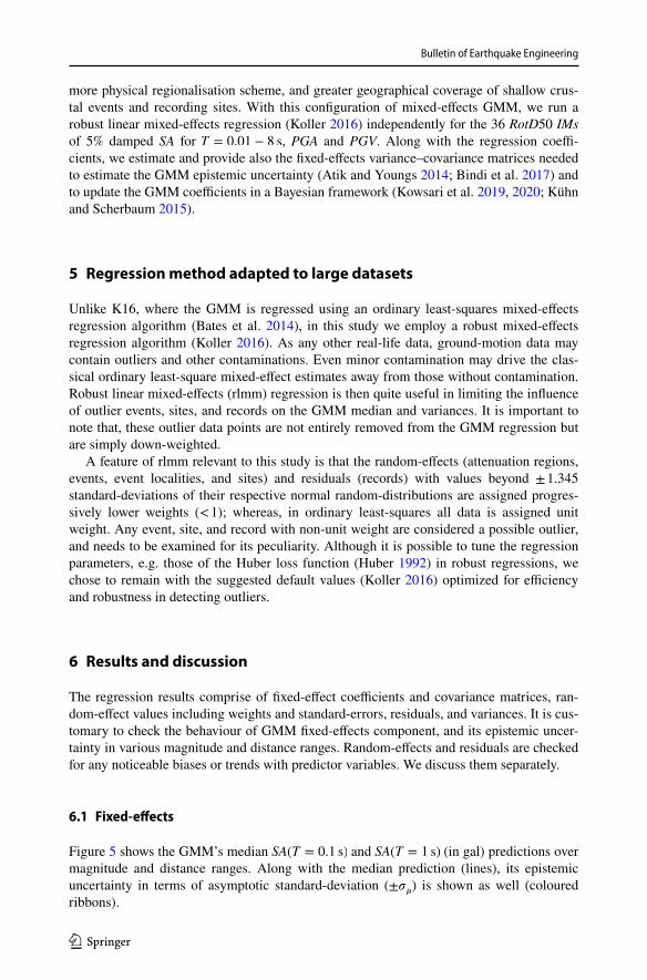
more physical regionalisation scheme, and greater geographical coverage of shallow crus-tal events and recording sites. With this configuration of mixed-effects GMM, we run a robust linear mixed-effects regression (Koller 2016) independently for the 36 RotD50 IMs of 5% damped SA for T = 0.01 − 8 s , PGA and PGV. Along with the regression coeffi-cients, we estimate and provide also the fixed-effects variance–covariance matrices needed to estimate the GMM epistemic uncertainty (Atik and Youngs 2014; Bindi et al. 2017) and to update the GMM coefficients in a Bayesian framework (Kowsari et al. 2019, 2020; Kühn and Scherbaum 2015).

5 Regression method adapted to large datasets

Unlike K16, where the GMM is regressed using an ordinary least-squares mixed-effects regression algorithm (Bates et al. 2014), in this study we employ a robust mixed-effects regression algorithm (Koller 2016). As any other real-life data, ground-motion data may contain outliers and other contaminations. Even minor contamination may drive the clas-sical ordinary least-square mixed-effect estimates away from those without contamination. Robust linear mixed-effects (rlmm) regression is then quite useful in limiting the influence of outlier events, sites, and records on the GMM median and variances. It is important to note that, these outlier data points are not entirely removed from the GMM regression but are simply down-weighted.

A feature of rlmm relevant to this study is that the random-effects (attenuation regions, events, event localities, and sites) and residuals (records) with values beyond ± 1.345 standard-deviations of their respective normal random-distributions are assigned progres-sively lower weights (< 1); whereas, in ordinary least-squares all data is assigned unit weight. Any event, site, and record with non-unit weight are considered a possible outlier, and needs to be examined for its peculiarity. Although it is possible to tune the regression parameters, e.g. those of the Huber loss function (Huber 1992) in robust regressions, we chose to remain with the suggested default values (Koller 2016) optimized for efficiency and robustness in detecting outliers.

6 Results and discussion

The regression results comprise of fixed-effect coefficients and covariance matrices, ran-dom-effect values including weights and standard-errors, residuals, and variances. It is cus-tomary to check the behaviour of GMM fixed-effects component, and its epistemic uncer-tainty in various magnitude and distance ranges. Random-effects and residuals are checked for any noticeable biases or trends with predictor variables. We discuss them separately.

6.1 Fixed‑effects

Figure 5 shows the GMM’s median SA(T = 0.1 s) and SA(T = 1 s) (in gal) predictions over magnitude and distance ranges. Along with the median prediction (lines), its epistemic uncertainty in terms of asymptotic standard-deviation ( ±�� ) is shown as well (coloured ribbons).


1 3

6.1.1 Distance scaling

First, we discuss the predicted SA(T = 0.1 s) and SA(T = 1 s) scaling with RJB in the left panel of Fig. 5. Looking at the curves for M4, we notice the impact of depth-dependent hD in rendering a shorter near-source saturation (plateau ~ 0 to 3 km) for shallower events, compared to the intermediate depth events (plateau ~ 0 to 5 km) and deeper events (pla-teau ~ 0 to 10 km). The three curves merge at about 30 km, which is our Rref. Beyond Rref = 30 km , the depth-dependence of distance scaling is non-existent. The predictions show good agreement with the non-parametric trends in Fig. 4.

Beyond the Rref, we see the region-dependent anelastic adjustments coming into play, which show the impact of adjusting c3 with �c

3,r = 0,−�c3,+�c3 . A region with faster than average attenuation will have a c

3,r more negative (with �c3,r = −�c3 ) than generic average,

and vice versa for slower attenuation (with �c3,r = +�c3 ). Which of the 46 regions in pan-

Europe apparently attenuate faster or slower than pan-European average (with �c3,r = 0 )

will be discussed in the following sections, and elaborated in a follow-up study. Effect of

Fig. 5 GMM median predictions of SA(T = 0.1 s) and SA(T = 1 s) . The left panel shows predicted scaling of SA(T = 0.1 s) . (top row) and SA(T = 1 s) (bottom row) with distance, for shallow (D < 10 km) , interme-diate (10 km ≤ D < 20 km) , and deep (20 km ≤ D) events in regions with average, slower, and faster than median anelastic decay at long distances. The right panel shows scaling of ground-motion with magnitude for the same combinations. In both panels, the epistemic uncertainty on GMM median is shown by the orange ribbon around prediction for intermediate depth events in average attenuating regions. Also shown are ground-motion observations corrected for �L2Ll, �B0

e,l , and �S2SS random-effects as grey markers


1 3

�c3,r at Rref < 30 km is negligible, as it should be. The 27 curves appear as three on either

side of Rref = 30 km , because near-source (hD) and far-source ( �c3,r ) adjustments have their

exclusive domains of influence.In Fig. 5, we also show the epistemic uncertainty on median predictions. The orange

ribbon is almost too thin to be noticeable for M4 and M5.5 predictions. Only for M7 and larger events, the ribbon is visibly wide because of the limited data from large magnitude events at near-source distances in the ESM dataset, and the uncertainty on the coefficient b3, which describes the magnitude scaling beyond Mh = 6.2.

6.1.2 Magnitude scaling

In the right panels of Fig. 5 we show the SA(T = 0.1 s) and SA(T = 1 s) scaling with MW. Here as well we show 27 curves, but this time for RJB = 10, 50, 150 km instead of the three MW values. The features in scaling with distance discussed in reference to the left panels also prevail here; �c

3,r is effective at RJB = 150 km , while hD is effective at RJB = 5 km , and neither are at RJB = 50 km . More important in this context, is the difference in scaling with magnitude at RJB = 10 km compared to RJB = 50, 150 km . Evidently, the scaling of SA(T = 0.1 s) is more gradual (less steep) at near-source distance for MW < Mh and over-saturates for MW ≥ Mh . This is a known physical behaviour wherein, near-source ground-motions, especially the short period SAs, are less sensitive to MW (Campbell 1981; Schme-des and Archuleta 2008). A few previous GMMs observed the same with various datasets. Boore et al. (2014) and K16 allowed oversaturation at large magnitudes ( MW ≥ 6.75) , but whether this is realistic or not needs to be verified with specially compiled near-source ground-motion datasets, e.g. the one recently made available by Pacor et al. (2018). The oversaturation effect, however, disappears at longer periods, as shown here for SA(T = 1 s).

Figure 6 shows the predicted response spectra for the same scenarios shown in Fig. 5. The effect of event depth and regionalized anelastic attenuation are the same as in Fig. 5. An interesting feature is that the peak of the response spectra shifts towards longer peri-ods for larger magnitude events, reflecting the decreasing corner-frequency with increasing magnitude of a Brune (1970) source spectra.

Fig. 6 Predicted response spectra of the GMM for various scenarios, differentiated by colour for shal-low ( D < 10 km ), intermediate ( 10 km ≤ D < 20 km ), and deep ( 20 km ≤ D ) events in the left panel. In the right panel are the response spectra differentiated by regional anelastic attenuation (Slower, Average, Faster)


1 3

An oddity in the response spectra is the kink appearing between T = 3.5 s and T = 4.5 s , which is most likely from the sudden loss of approximately 3000 usable records (in regres-sion) due to the high-pass filtering frequency criterion #5 in Ground-Motion Data and Selection Criteria. Similar kinks can be seen in a few other subsequent plots as well. Tra-ditionally, GMM fixed-effect regression coefficients are smoothened in a post-processing step, in order to smoothen the predicted response spectra and to constrain the GMM behav-iour in sparsely sampled magnitude-distance ranges, e.g. Abrahamson et al. (2014). How-ever, in this study we chose not to alter the fixed-effect coefficients, and to maintain full consistency with their variance–covariance matrices; which will be necessary in testing and updating of the GMM.

6.2 Random‑effects and residuals

Figure 7 shows the random-effect and residual standard-deviations of the GMM. The total ergodic standard-deviation of the GMM is � =

√�2L2L

+ �20+ �2

S2S+ �2 , when considering

all source and site variabilities as aleatory. The solid lines in this plot correspond to the variance estimates of the GMM from ESM dataset (this study), while the dashed lines indi-cate those of the K16 GMM from RESORCE dataset. Note that the K16 GMM does not regionalise the events, and thus between-locality variability component �L2L is absent. For the sake of comparison between the two models, we combine the two source related ran-dom-variances of this study into the traditional between-event variability � =

√�2L2L

+ �20

We show that the total standard-deviation σ of the new GMM is considerably larger than that of K16 GMM. The largest increase in σ is at short-moderate periods, and is from the increase in between-event τ and between-site �S2S variabilities. The increase in between-event variability can be attributed to the increased regional diversity of earthquakes, the increase of number of 4 ≤ MW ≤ 5.5 events from 164 in RESORCE to 778 in ESM, and the additional 76 events with 3 ≤ MW < 4 in ESM. Between-site variability is clearly from the increase in number of recording sites from 385 in RESORCE to 1829 in ESM. The residual variability � of the new GMM, however, is equal or smaller than that of K16, despite the increase in regional diversity, the sample size, and the recording distance range

Fig. 7 Residual and random-effect variance estimates of the GMM for T = 0.01 − 8 s (solid lines). The colours identify the various random-effect and resid-ual components. For comparison, variance estimates for the K16 GMM from RESORCE dataset (Kotha et al. 2016) are overlain in dashed lines


1 3

from 300 to 545 km. In our view, this plot emphasizes the need to move from ergodic to partially non-ergodic region- and site-specific ground-motion predictions to inhibit the effect of increased σ on PSHA (Anderson and Brune 1999; Bommer and Abrahamson 2006; Kotha et al. 2017; Rodriguez-Marek et al. 2013).

6.2.1 Anelastic attenuation variability

Figure 8 shows the region-specific �c3,r adjustments (coloured lines and ribbons) of the

45 regions for T = 0.01 − 8 s . Most of these curves lay within the ±�c3 (red lines) bounds. As indicated by �c3 , the region-to-region variability of apparent anelastic attenuation is the highest at short periods, and decreases gradually towards longer periods. High-frequency ground-motions are more susceptible to strong anelastic decay in the crust, which could be related to the crustal properties. Long period SAs are not effected as much by anelastic attenuation, therefore regional differences are relatively smaller, and �c3 is smaller by ~ 50% at T ≥ 1 s.

In RESORCE dataset, K16 observed that short period SAs attenuate faster in Italy than in Turkey, which was observed earlier in NGA-West2 dataset by Boore et al. (2014), and confirmed later in Fourier domain by Bora et al. (2017). However, these observations were based on distinguishing regions by administrative boundaries and not geological or geophysical features. Since �c3 estimated from the new regionalisation is not zero, we can assert that regional variability of anelastic attenuation exists. Of course, regions with fewer data have larger epistemic uncertainty (standard-error) on their δc

3,r , but the largest epis-

temic uncertainty is always lower than the aleatory τc3

, and decreases with increasing data.Figure 9 shows the spatial variability of apparent anelastic attenuation as captured by

the regionalisation model of Fig. 2. In this figure, red polygons identify regions with slower than pan-European average of anelastic attenuation c3 i.e. δc

3,r> 0 , and δc

3,r< 0 for the

faster attenuating blue regions. Regions with insufficient data, and thereby large epistemic uncertainty on their δc

3,r , are white in color, and given δc

3,r= 0 . There are few interesting

features in these maps:

1. Regions with similar attenuation characteristics are spatially clustered, although this is period dependent. In general, regions characterized with high seismic activity (e.g. Italy

Fig. 8 δc3,r

for T = 0.01 − 8 s . Each line corresponds to one of the 46 attenuation regions, with colours indicating their weight in robust regression. Overlain red curves mark the ±τ

c3 values.

Regions with δc3,r

(T) beyond ±1.345τ

c3(T) are given lower than a unit weight


1 3

and Greece) show strong attenuation compared to those with lower seismic activity (e.g. central Europe).

A Bayesian clustering of regions with similar attenuation characteristics is proposed in the companion paper by Weatherill et al. (2020c); wherein, similar regions (r) are clustered (cl) and assigned cluster-specific δc

3,cl with lower standard-error and smaller

cluster-specific τc3,cl

. The epistemic uncertainty (standard-error) on cluster-specific δc3,cl

is smaller than that of δc

3,r due to the accumulation of data from multiple regions; while

the cluster-specific τc3,cl

is smaller than the overall τc3

due to a smaller within-cluster variability of region-specific δc

3,r

2. The best-sampled regions are in central Italy with 5703 records from Northern and cen-tral Apennines W (West), 3438 records from Northern and central Apennines E (East). While attenuating faster than the pan-European average, there appears to be a strong contrast between these adjacent regions

Fig. 9 Variation of �c3,r across the 46 attenuating regions (r) for T = 0.1 s (top panel) and T = 1 s (bottom

panel). Blue polygons identify regions with anelastic attenuation faster than the pan-European average, red polygons locate regions with slower attenuation, and white polygons are regions close to the average. Regions with fewer ground-motion observations, thereby larger epistemic error on �c

3,r , are more transpar-ent and appear white. Note that the color scale is limited to vary between ±3 ∗ �c3(T) for each period T


1 3

3. The fastest attenuation in the Aegean Sea is observed in the Gulf of Corinth, where the sites record highly attenuated ground-motions traversing across the Aegean volcanic arc

A contrast in short period attenuation is apparent around the Alps regions. In addition, some differences are noticeable between west, north, and central Anatolia. Although not conclusive, rapidly changing crustal thickness (Grad et al. 2009) and associated crustal properties may partially explain the rapid change in attenuation properties in these regions. Regional variability of anelastic attenuation may in fact be a combination of variability of crustal shear-wave velocity, crustal quality factor (e.g. coda Q), mantle temperature influ-encing the rigidity of the crust, and other parameters. Further elaboration is preferred in Fourier domain, rather than with response spectra here, in a follow-up study.

6.2.2 Source variability

Earthquake source variability is split in two random-effect groups: between-event ΔB0

e= N

(0, �2

0

) and between-locality ΔL2L = N

(0, �2

L2L

) . Between-event terms can be

estimated for the recorded earthquakes, but are difficult to predict for prospective earth-quakes because of their spatiotemporal variability. Even when correlated with stress-drop or a source parameter that can explain the relative differences in ground-motions, predic-tion of stress-drop for the next event is not yet possible. Traditionally therefore, between-event variability is considered purely aleatory. Between-locality random-effect is intended to quantify a portion of the between-event spatial variability into tectonic localities.

Figure 10 shows the �L2Ll(T = 0.01 − 8 s) for 56 tectonic localities. As always, the standard-error (or epistemic uncertainty) of �L2Ll values is smaller than the �L2L . �L2L val-ues are non-negligible, and the GMM fit improves (based on analysis of variance) with introduction of between-locality random-effect group. Therefore, we consider it an effec-tive random-effect grouping. Although it is tempting to relate �L2Ll to some source param-eter, it is preferably done in the Fourier domain in a follow-up study.

Figure 11 maps the various tectonic localities (indexed l) color coded to their δL2Ll(T = 0.1 s) and δL2Ll(T = 1 s) values. In the top panel, corresponding to δL2Ll(T = 0.1 s) , a clear difference between central Italy and north-western Anato-lia can be seen. Apparently, earthquakes located in central Apennine region produce substantially lower short period ground-motions than those in north-western Anatolia.

Fig. 10 δL2Ll for T = 0.01 − 8 s . Each line corresponds to one of the 56 tectonic localities, with colours indicating their weight in robust regression. Overlain red curves mark the ±τL2L values. Tectonic localities with δL2Ll(T) beyond ±1.345τL2L(T) are given a lower weight than one


1 3

Similarly, there is an apparent distinction between the central Apennines and Po-plain earthquakes. The central Apennines tectonic locality contains the recent M6.5 Nor-cia earthquake (2016) and associated shocks, and several historic earthquakes in that region. The Po-plain locality contains data from the substantially stronger M6.45 Friuli earthquake (1976) and a few recent earthquakes. At a first glance, it may appear as if the spatial patterns are due to the predominant focal mechanisms in the regions, but the diversity of focal mechanisms within each region (especially among smaller events) dis-suades this hypothesis. Spectral decomposition of the ESM dataset by Bindi and Kotha (2020) revealed a much larger stress-drop of the M6.45 Friuli earthquake compared to M6.5 Norcia earthquake—the δL2Ll of regions containing these earthquakes also con-trast similarly (Bindi et al. 2019). Once again, correlating the random-effects obtained in response spectra domain (as here) to the earthquake parameters (such as stress-drop)

Fig. 11 Variation of �L2Ll across the 56 tectonic locality (l) for T = 0.1 s (top panel) and T = 1 s (bottom panel). Blue polygons identify tectonic localities that produced earthquakes less energetic than the pan-European average, red polygons identify localities with more energetic earthquakes, and white polygons are localities close to the average. Tectonic localities with fewer ground-motion observations, thereby larger epistemic error on �L2Ll , are more transparent and appear white. Note that the color scale is limited to vary between ±3 ∗ �L2L(T) for each period T


1 3

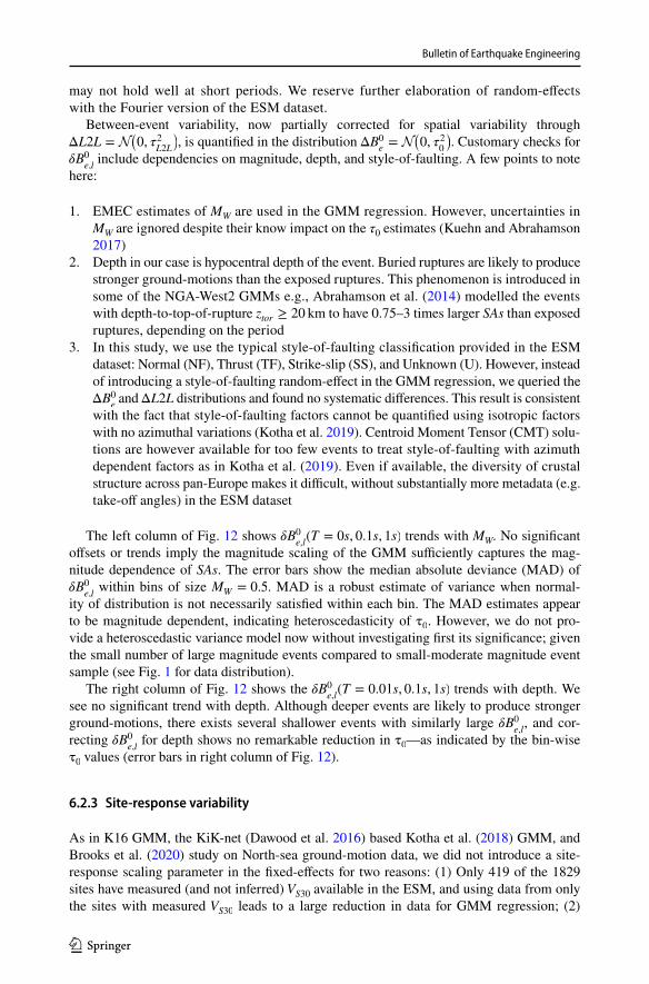
may not hold well at short periods. We reserve further elaboration of random-effects with the Fourier version of the ESM dataset.

Between-event variability, now partially corrected for spatial variability through ΔL2L = N

(0, �2

L2L

) , is quantified in the distribution ΔB0

e= N

(0, �2

0

) . Customary checks for

�B0

e,l include dependencies on magnitude, depth, and style-of-faulting. A few points to note

here:

1. EMEC estimates of MW are used in the GMM regression. However, uncertainties in MW are ignored despite their know impact on the τ0 estimates (Kuehn and Abrahamson 2017)

2. Depth in our case is hypocentral depth of the event. Buried ruptures are likely to produce stronger ground-motions than the exposed ruptures. This phenomenon is introduced in some of the NGA-West2 GMMs e.g., Abrahamson et al. (2014) modelled the events with depth-to-top-of-rupture ztor ≥ 20 km to have 0.75–3 times larger SAs than exposed ruptures, depending on the period

3. In this study, we use the typical style-of-faulting classification provided in the ESM dataset: Normal (NF), Thrust (TF), Strike-slip (SS), and Unknown (U). However, instead of introducing a style-of-faulting random-effect in the GMM regression, we queried the ΔB0

e and ΔL2L distributions and found no systematic differences. This result is consistent

with the fact that style-of-faulting factors cannot be quantified using isotropic factors with no azimuthal variations (Kotha et al. 2019). Centroid Moment Tensor (CMT) solu-tions are however available for too few events to treat style-of-faulting with azimuth dependent factors as in Kotha et al. (2019). Even if available, the diversity of crustal structure across pan-Europe makes it difficult, without substantially more metadata (e.g. take-off angles) in the ESM dataset

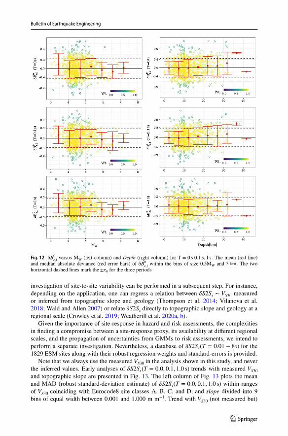
The left column of Fig. 12 shows �B0

e,l(T = 0s, 0.1s, 1s) trends with MW. No significant

offsets or trends imply the magnitude scaling of the GMM sufficiently captures the mag-nitude dependence of SAs. The error bars show the median absolute deviance (MAD) of �B0

e,l within bins of size MW = 0.5 . MAD is a robust estimate of variance when normal-

ity of distribution is not necessarily satisfied within each bin. The MAD estimates appear to be magnitude dependent, indicating heteroscedasticity of τ

0 . However, we do not pro-

vide a heteroscedastic variance model now without investigating first its significance; given the small number of large magnitude events compared to small-moderate magnitude event sample (see Fig. 1 for data distribution).

The right column of Fig. 12 shows the �B0

e,l(T = 0.01s, 0.1s, 1s) trends with depth. We

see no significant trend with depth. Although deeper events are likely to produce stronger ground-motions, there exists several shallower events with similarly large �B0

e,l , and cor-

recting �B0

e,l for depth shows no remarkable reduction in τ

0—as indicated by the bin-wise

τ0 values (error bars in right column of Fig. 12).

6.2.3 Site‑response variability

As in K16 GMM, the KiK-net (Dawood et al. 2016) based Kotha et al. (2018) GMM, and Brooks et al. (2020) study on North-sea ground-motion data, we did not introduce a site-response scaling parameter in the fixed-effects for two reasons: (1) Only 419 of the 1829 sites have measured (and not inferred) VS30 available in the ESM, and using data from only the sites with measured VS30 leads to a large reduction in data for GMM regression; (2)


1 3

investigation of site-to-site variability can be performed in a subsequent step. For instance, depending on the application, one can regress a relation between �S2Ss ∼ VS30 measured or inferred from topographic slope and geology (Thompson et al. 2014; Vilanova et al. 2018; Wald and Allen 2007) or relate �S2Ss directly to topographic slope and geology at a regional scale (Crowley et al. 2019; Weatherill et al. 2020a, b).

Given the importance of site-response in hazard and risk assessments, the complexities in finding a compromise between a site-response proxy, its availability at different regional scales, and the propagation of uncertainties from GMMs to risk assessments, we intend to perform a separate investigation. Nevertheless, a database of �S2Ss(T = 0.01 − 8s) for the 1829 ESM sites along with their robust regression weights and standard-errors is provided.

Note that we always use the measured VS30 in the analysis shown in this study, and never the inferred values. Early analyses of �S2Ss(T = 0.0, 0.1, 1.0 s) trends with measured VS30 and topographic slope are presented in Fig. 13. The left column of Fig. 13 plots the mean and MAD (robust standard-deviation estimate) of �S2Ss(T = 0.0, 0.1, 1.0 s) within ranges of VS30 coinciding with Eurocode8 site classes A, B, C, and D, and slope divided into 9 bins of equal width between 0.001 and 1.000 m m−1. Trend with VS30 (not measured but)

Fig. 12 δB0

e,l versus MW (left column) and Depth (right column) for T = 0 s 0.1 s, 1 s . The mean (red line)

and median absolute deviance (red error bars) of δB0

e,l within the bins of size 0.5M

W and 5 km . The two

horizontal dashed lines mark the ±τ0 for the three periods


1 3

inferred from a VS30 ∼ slope correlation model of Wald and Allen (2007) is comparable to the trend with slope from which it is inferred in the right column of Fig. 13.

The correlation �S2Ss ∼ VS30 (measured only) at short-periods T = 0.0, 0.1 s is rather poor, as indicated by similar mean and MAD (the robust standard-deviation) for VS30 < 800m/s in the left column of Fig. 13. It appears that short-period site-responses of soft rock, stiff, and soft soils (EC8 class B, C, D) in this dataset are not adequately distinguishable. However, it is interesting to see that the mean of EC8 class A ‘rock’ sites with VS30 ≥ 800m/s is much lower than the rest, along with a considerably larger vari-ability. Short-period linear soil-response of rock sites is known to be highly variable com-pared to softer soils, whose nonlinear soil-response may suppress the otherwise high variability from linear-only amplification (Bazzurro and Cornell 2004). On the contrary, the long-period site-response of rock sites is less variable than that of softer soils (e.g. 180m/s ≤ VS30 < 800m/s) . Similar inferences can be drawn from the �S2Ss ∼ slope plots in the right column of Fig. 13, where higher slopes are (usually) indicative of rock sites on steep hillsides, and lower slopes at softer sites located on flatter sediments.

Fig. 13 Plot showing the trend of δS2Ss(T = 0, 0.1, 1 s) (from top to bottom rows) with V

S30 (left column)

and topographic slope at site location (right column). Note that, only 419 sites have measured VS30

, com-pared to 1829 sites with slope. At short-moderate periods (T = 0, 0.1 s), the binned mean and MAD (red error bars) show a poor non-parametric trend, which improves at longer periods (T = 1 s). The blue line represents the parametric forms (Eqs. 6 and 7) fit to the data


1 3

For completeness, along with a database of �S2Ss(T = 0.0 − 8.0 s) for the 1829 ESM sites, we derive a continuous empirical models for both �S2Ss ∼ VS30(measured) and �S2Ss ∼ slope correlations seen in Fig. 13. We chose a quadratic functional form instead of the traditional piecewise linear function; as shown in Eqs. (6) and (7). Here, the measured VS30 is in m s−1 and slope in m m−1, the regression coefficients g

0, g

1, g

2 are different for

SRVs30 and SRslope , and change with period. The residuals from �S2Ss ∼ VS30 (measured) and �S2Ss ∼ slope regressions are �S2SVS30

s and �S2Sslopes , with robust standard-deviations �VS30

S2S

and �slope

S2S , respectively.

Robust linear fits using an M estimator (Venables and Ripley 2002), at each of 34 peri-ods between T = 0.01s − 8 s,PGA(T = 0 s) and PGV, are derived for δS2S

s∼ VS30 cor-

relation of 419 sites with measured VS30 available, and δS2Ss∼ slope of the 1829 sites

with slope derived from digital elevation models provided by Shuttle Radar Topography Mission.

Although heteroscedastic models of �VS30

S2S and �slope

S2S appear reasonable in Fig. 13, we

chose not to propose one without testing its significance; given the uneven distribution of sites in different bins. Figure 13 shows the reduction in between-site variance from using VS30 and slope as site-response proxies (Eqs. 6 and 7) in the GMM. For comparison, the variances of K16 GMM are also shown in this plot. Note that the K16 GMM comes in two variants: one without a site-response component, and another with measured VS30 as a proxy for linear site-response. Note that, the K16 standard-deviations shown in Fig. 7 are those when not using VS30 as a parameter, while those in Fig. 14 are when using VS30 as site-response proxy—hence, lower in the latter.

(6)SRVs30 = g0+ g

1⋅ ln

(VS30

800

)+ g

2⋅

(ln

(VS30

800

))2

(7)SRslope = g0+ g

1⋅ ln

(slope

0.1

)+ g

2⋅

(ln

(slope

0.1

))2

Fig. 14 Between-site and total variance estimates (�S2S, �) of the GMM for T = 0.01–8 s (solid lines) compared with those of K16 GMM from RESORCE dataset (dashed lines). Reduc-tion of ( �S2S, �) to (�VS30

S2S, �VS30 )

using VS30 , and to (�slope

S2S, �slope)

using Slope as site-response proxies is shown here. Note that the (�S2S, �) of K16 GMM are those using VS30 as site-response proxy, and are smaller than those shown in Fig. 7, which are from the K16 GMM version without a site-response parameter


1 3

A significant reduction in between-site standard-deviation can be achieved using an efficient site-response proxy or a combination of proxies. Since only a few sites are pro-vided with measured VS30 values, �VS30

S2S is substantially smaller than �slope

S2S . For a new site

with VS30 or slope available, Eq. (6) or (7) can be appended to the ln(�) in Eq. (2), while replacing �S2S (when estimating σ) with �VS30

S2S or �slope

S2S , respectively. For site with nei-

ther site-response proxy available, but with sufficient strong ground-motion recordings, the site-specific �S2Ss term can be estimated and used for site-specific ground-motion predictions.

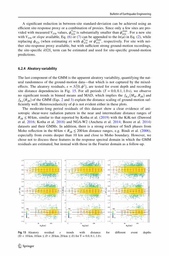
6.2.4 Aleatory variability

The last component of the GMM is the apparent aleatory variability, quantifying the nat-ural randomness of the ground-motion data—that which is not captured by the mixed-effects. The aleatory residuals, � = N

(0,�2

), are tested for event depth and recording

site distance dependencies in Fig. 15. For all periods ( T = 0.0, 0.1, 1.0 s ), we observe no significant trends in binned means and MAD, which implies the fR,g

(MW ,RJB

) and

fR,a(RJB

) of the GMM (Eqs. 2 and 3) explain the distance scaling of ground-motion suf-

ficiently well. Heteroscedasticity of � is not evident either in these plots.The moderate-long period residuals of this dataset show a clear evidence of ani-

sotropic shear-wave radiation pattern in the near and intermediate distance ranges of RJB ≤ 80 km , similar to that reported by Kotha et al. (2019) with the KiK-net (Dawood et al. 2016; Kotha et al. 2018) and NGA-W2 (Ancheta et al. 2014; Boore et al. 2014) datasets and their GMMs. In addition, there is a strong evidence of SmS phases from Moho reflection in the 60 km < RJB ≤ 200 km distance ranges, e.g. Bindi et al. (2006), especially from events deeper than 10 km and close to Moho boundary. However, we chose not to discuss these features in the response spectral domain in which the GMM residuals are estimated, but instead with those in the Fourier domain as a follow-up.

Fig. 15 Aleatory residual ε trends with distance for different event depths ( D < 10 km, 10 km ≤ D < 20 km, 20 km ≤ D ) for T = 0.0, 0.1, 1.0 s


1 3

7 Application

The GMM presented in this study has no new explanatory parameters in its functional form compared to previous pan-European GMMs. The median predictions rely only on the two generic parameters MW and RJB, which constitute the fixed-effects. Of course, the standard-deviation estimates of the new model are significantly larger than those of K16, but this is to be expected given the 15-fold increase in data: from a greater variety of sites, tectonic locali-ties, MW ≤ 5.5 events, etc. To explain the variability, without introducing new parameters, we instead resolved the apparent aleatory variability into various possible contributions. There-fore, the model can be used ignoring the region-to-region, locality-to-locality, and site-to-site variabilities, but at the cost of increased aleatory variability. We provide three application possibilities:

7.1 Ergodic application

The first approach is by ignoring all repeatable effects, i.e. the region, locality, and site-spe-cific adjustments. The between-locality, between-event, between-site, residual standard-devia-tions can be combined into an ergodic, total standard-deviation � =

√�2L2L

+ �20+ �2

S2S+ �2 ,

as shown in Fig. 7. In this case, the regional differences in anelastic attenuation, quantified by �c3 , will be treated as an epistemic uncertainty on far-source distance scaling. The epistemic uncertainty on the regionalised anelastic attenuation coefficient c3 in Eq. (4) is �c3 . This uncer-tainty can be handled with a GMM logic tree consisting of a slower

(c3,r = c

3+ �.�c3

) , aver-

age (c3,r = c

3

) , and faster

(c3,r = c

3− �.�c3

) attenuating branches. Following the Miller III

and Rice (1983) three point approximation of a Gaussian distribution, with � ≈ 1.732 one can use logic tree branch weights of 0.167, 0.666, and 0.167, respectively for slower, average, and faster branches. Consequently, the ground-motion prediction is a weighted mixture of three Gaussian distributions N

(ln(�), �2

) , where ln(�) is estimated from Eq. (2) for three values of

c3,r ∈

(c3, c

3+ � ⋅ �c3, c3 − � ⋅ �c3

).

Within the context of an ergodic application, if a site has either the measured VS30 or slope information available, but no site-specific ground-motion recordings, then the �S2S in the esti-mation of � =

√�2L2L

+ �20+ �2

S2S+ �2 can be replaced with �VS30

S2S and �slope

S2S , whilst append-

ing the fixed-effects of Eq. (2) with Eqs. (6) and (7), respectively. Figure 14 shows the conse-quent reduction of σ to �VS30 and �slope values, when using site-response proxies VS30 and slope, respectively. Consequently, the ground-motion predictions follow the mixed Gaussian distri-bution N

(ln(�) + SRVs30 , �VS30

2) or N

(ln(�) + SRslope, �slope2

) , where ln(�) is estimated

from Eq. (2) for three values of c3,r ∈

[c3, c

3+ � ⋅ �c3, c3 − � ⋅ �c3

] , and SRVs30 or SRslope are

estimated from Eq. (6) or (7). The reduced aleatory variability from using a site-response proxy is beneficial until when enough ground-motion data can be collected at a site, and then �S2Ss for the new site can be estimated using equations provided in Kotha et al. (2017); Rodri-guez-Marek et al. (2013); Sahakian et al. (2018); Villani and Abrahamson (2015), etc.

7.2 Region‑specific application

For region-specific applications, the predictions can be upgraded with the region-specific anelastic attenuation and tectonic locality specific adjustments. Anelastic attenuation is regionalised by adjusting the generic coefficient c3 in Eq. (4) with a region-specific value


1 3

�c3,r , as in c

3,r = c3+ �c

3,r, where region r is decided by the location of the site. Since �c3,r

are estimated from a smaller region-specific sample of ground-motion recordings, it should be treated as epistemically uncertain. For this purpose, standard-error on �c

3,r are pro-vided as well, and these are always smaller than �c3 . Treating the SE

(�c

3,r

) as uncertainty

on mean of a normally distributed sample, the 95% confidence interval of �c3,r would be

�c3,r ± 1.6SE

(�c

3,r

).

Similarly, depending on the tectonic locality of the earthquake, the GMM predictions can be further regionalised by adjusting e1 in Eq. (2) to e

1,l = e1+ �L2Ll , where l identifies

locality tectonic locality of the earthquake. Since �L2Ll is estimated from a smaller local-ity-specific ground-motion sample, the 95% confidence interval is bounded by �L2Ll ± 1.6.SE

(�L2Ll

) . A reduction of up to 10% in σ is achieved by dropping the �L2L

from aleatoric variance, resulting in a smaller �r =√

�20+ �2

S2S+ �2 , as shown in Fig. 16.

Further reductions to �Sloper are �Vs30

r possible if the site-response scaling with slope and Vs30 (Eqs. 6 and 7) are used in predictions, respectively.

It is interesting to compare the total standard-deviation σ (dashed line in Fig. 16) of the regionalised, Vs30 based K16 GMM with �Vs30

r of this study. At T ≤ 0.3s , the �Vs30

r is about 6% larger than its K16 counterpart; while at T > 0.3 s, �Vs30

r is as much as 14% smaller. Despite the enormous increase in data, it appears that regionalisation has helped in sub-stantially curtailing the increase in apparent aleatory variability.

7.3 Region‑ and site‑specific application

Partially non-ergodic region- and site-specific ground-motion predictions are possible for those sites with �S2Ss provided with this GMM or for new sites with sufficient ground-motion data. �S2Ss for the 1829 sites in the ESM dataset are provided, along with the �c

3,r

Fig. 16 Reduction in total standard deviation estimates (σ) of the GMM for T = 0.01–8 s (solid lines) from ergodic with and without site-response proxy, region-specific with and without site-response proxy, and region- and site-specific values. Standard deviation estimates when using site-response proxies are indi-cated by the annotations with corresponding superscript, i.e. ( �VS30 ) with VS30 , and to ( �slope) with slope. Annotations with subscript r correspond to the variances for regionalized predictions, i.e. from discounting region-to-region variability �L2L from σ. Values annotated with subscript r, s correspond to region- and site-specific predictions discounting also the �S2S . The black dashed line is the total standard-deviation (same as in Fig. 14) of the regionalized and Vs30 based Kotha et al. (2016) GMM, and compares with the �VS30

r of this study


1 3

of their region, and �L2Ll of nearby tectonic localities (earthquake sources). Since between-site and between-locality variabilities do not apply for site-specific predictions, the reduc-tion in apparent aleatory variability is enormous, i.e. �r,s =

√�20+ �2 is about 40% smaller

than � =

√�2l2l

+ �20+ �2

S2S+ �2 , as shown in Fig. 16. However, the reduction in aleatory

variability will be accompanied by additional epistemic uncertainty. In addition to those in region-specific predictions, uncertainty on (the mean) �S2Ss should be accounted with ±1.6.SE

(�S2Ss

). Region- and site-specific predictions therefore are a mixture of 27 Gauss-

ian distributions N(ln(�r,s

), �2

r,s

) , where ln

(�r,s

) is estimated from Eq. (1) for three values

of c3,r ∈

[c3+ �c

3,r, c3 + �c3,r + 1.6SE

(�c

3,r

), c

3+ �c

3,r − 1.6SE(�c

3,r

)] , three values of

e1,l,s ∈

[e1,l + �S2Ss, e1,l + �S2Ss + 1.6SE

(�S2Ss

), e

1,l + �S2Ss − 1.6SE(�S2Ss

)], wherein

e1,l ∈

[e1+ �L2Ll, e1 + �L2Ll + 1.6SE

(�L2Ll

), e

1+ �L2Ll − 1.6SE

(�L2Ll

)].

In complement, a more practical application is presented in the companion study by Weatherill et al. (2020c), where a more thorough comparison of this GMM with contempo-rary models is provided. Weatherill et al. (2020c) also provides a more complete discussion on how the various epistemic uncertainties in this GMM can be handled in the logic tree framework of a PSHA.

7.4 Towards non‑ergodic ground‑motion predictions

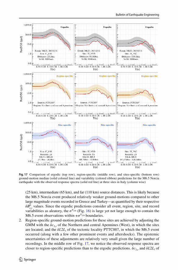
For tectonic localities, attenuating regions, and sites with sufficient amount of recordings the epistemic uncertainty on the random-effect adjustments are negligible with respect to the random-effect and standard-deviations. Collecting more ground-motion recordings is principal in moving towards non-ergodic predictions. The benefits in resolving the ergodic assumption and progressing towards region- and site-specific in ground-motion prediction is demonstrated Fig. 17. In this plot, predictions for the M6.5 Norcia event of the central Italy sequence, which occurred on 30th October, 2016, are compared to the response spec-tra recorded at three sites covered by the Italian strong motion network (Gorini et al. 2010). These sites are identified by the network code IT in the ESM dataset: (1) permanent, free-field station LSS (Leonessa) with VS30 = 1091m/s located 25 km from the event epicentre, (2) permanent, free-field station MVB (Marsciano Monte Vibiano) with VS30 = 1046m/s located 65 km from the event epicentre and, (3) permanent, free-field station PSC (Pes-casseroli) with VS30 = 1000m/s located 110 km from the event epicentre. The three col-umns in Fig. 17 correspond to the three stations.

These event and stations are selected to demonstrate progressively (in Fig. 17) the impact of moving from ergodic prediction relying on VS30 as site-response proxy (top row), through region-specific predictions (middle row) considering regional (Northern and cen-tral Apennines West) anelastic attenuation ( c

3,r = c3+ �c

3,r ) and adjustment specific to the tectonic locality ( e

1,l = e1+ �L2Ll ) containing the event (locality ID: “PTTC007”), to

region- and site-specific predictions (bottom row) from an additional site-specific adjust-ment ( e

1,l,s = e1+ �L2Ll + �S2Ss ). Both the median prediction and standard-deviation

change in process, which is reflected by the width of the coloured ribbon in Fig. 17. The �S2Ss(T = 0.01 − 8s) of these sites are estimated from 29, 15, and 20 records from pre-dominantly small-moderate earthquakes (details in the Fig. 17 panels). A few comments on this figure:

1. The ergodic median predictions (central line) and one �VS30 interval (ribbon) are sys-tematically above the observed response spectra at the three rock sites, located at near


1 3

(25 km), intermediate (65 km), and far (110 km) source distances. This is likely because the M6.5 Norcia event produced relatively weaker ground-motions compared to other large magnitude events recorded in Greece and Turkey—as quantified by their respective �B0

e,l values. Since the ergodic predictions consider all event, region, site, and record

variabilities as aleatory, the �VS30 (Fig. 16) is large yet not large enough to contain the M6.5 event observations within ±�VS30 boundaries.

2. Region-specific ground-motion predictions for these sites are achieved by adjusting the GMM with the �c

3,r of the Northern and central Apennines (West), in which the sites are located; and the �L2Ll of the tectonic locality PTTC007, in which the M6.5 event occurred (along with a few other prominent events and aftershocks). The epistemic uncertainties of these adjustments are relatively very small given the large number of recordings. In the middle row of Fig. 17, we notice the observed response spectra are closer to region-specific predictions than to the ergodic predictions. �c

3,r and �L2Ll of

Fig. 17 Comparison of ergodic (top row), region-specific (middle row), and sites-specific (bottom row) ground-motion median (solid colored line) and variability (colored ribbon) predictions for the M6.5 Norcia earthquake with the observed response spectra (solid red line) at three sites in Italy (column wise)


1 3

these regions are both lower than the pan-European average (which is zero), meaning the region attenuates short-period ground-motions faster and the events on average produce weaker ground-motions than elsewhere in pan-European region.

It is interesting to note that, at short distances (site IT_LSS) the �c3,r has no effect on

region-specific predictions, and the shift is mostly from �L2Ll—and so is at intermediate distance (site IT_MVB). At far-source distances (site IT_PSC), the combined effect of �c

3,r and �L2Ll worked well to capture the observed response spectra within the narrower ±�

VS30

r (Fig. 16) range about the region-specific median.3. Region- and site-specific predictions (site-specific in short) for the three sites are shown

in the bottom row of Fig. 17. Along with the curves, details on the number of record-ings, magnitude and distance ranges (1st and 3rd quantile) of the recordings are pro-vided. The additional adjustment to the preceding region-specific predictions is through e1,l,s = e

1+ �L2Ll + �S2Ss . While most of the data in estimating the �S2Ss of these

sites is from small-moderate sized earthquakes, the site-specific predictions fit quite well with the observations for the large M6.5 event. Since �S2Ss are used to adjust the region-specific ground-motions, the VS30 becomes irrelevant, and �VS30

S2S is dropped from

�VS30

r resulting in a smaller �r,s.

In the above example, we demonstrated that applying region-specific adjustments noticeably improved the match between observations and predictions. The best agree-ment was clearly from using region- and site-specific adjustments. To substantiate this claim, we performed a 10-fold cross-validation exercise to verify if the introduction of the various random-effects into GMM functional form indeed improves its prediction capabilities. In doing so, we re-run the regression with three functional forms:

• Ergodic model with no regionalisation of anelastic attenuation, no localisa-tion of event terms, and no site-specific adjustments, i.e. no random-effects �c

3,r, �L2Ll, �S2Ss• Regional model with regionalisation of anelastic attenuation and tectonic localisa-

tion of events, leaving out the random-effect to capture site-to-site variability, i.e. only the random-effects �c

3,r and �L2Ll , but no �S2Ss• Site-specific model identical to the GMM presented here i.e., regionalisation of ane-

lastic attenuation, localisation event terms, and the site-to-site random-effect

To perform the cross-validation, the dataset is split into 10 parts with non-overlap-ping events. Meaning, earthquakes (and records) are exclusive to their subsets and do not feature in any other subset. We perform regression of the three models on any nine subsets combined, and test the predictions on the tenth subset. Root-mean-squared-errors are estimated for each trial and then averaged over the ten trials. This exercise is repeated for IMs:PGA,PGV , SA(T = 0.1, 0.2, 0.5, 1, 2, 4 s).

Figure 18 shows a histogram of RMSE for each IM, from the three models. The reduction in RMSE from ergodic to region-specific GMMs is clear and most prominent at short periods. Towards longer periods, the improvement is less pronounced but is still substantial. This is because the regionalisation random-effects are focused on the capturing variabilities in short-period ground-motions. In Fig. 7, we notice the overall variability σ peaks at short periods. In Figs. 8 and 10, the largest regional variability of anelastic attenuation �c3 and tectonic localities �L2L is also at short periods T ≤ 0.3 s . Without regionalisation, along with the increased the short period ground-motion


1 3

prediction variability and reduced precision of an ergodic median, the predictive capa-bility (measured as RMSE) of the GMM is reduced as well.

Across all the periods, i.e. the entire response spectra, the best predictive capabilities are those of region- and site-specific GMM. In Fig. 16, the largest reduction in σ is achieved not from using VS30 or slope as the site-response proxy, but from using �S2Ss as the site-specific adjustment. However, it is unlikely that every site has sufficient ground-motion data to estimate it’s site-specific �S2Ss . In that case, alternative site-response proxies are sought to predict the �S2Ss , as in Kotha et al. (2018); Weatherill et al. (2020b). However, even in these studies, while the long period site-response could be partially explained using some geotechnical parameters, short-period site-response is much more variable—even among the so-called reference rock sites (Bard et al. 2019; Pilz et al. 2020).

8 Summary

In this study, we present the update of the Kotha et al. (2016) region- and site-specific GMM, using the recently published European Strong Motion dataset (ESM) by Lanzano et al. (2019a) and Bindi et al. (2018b). The update derived from a dataset 15 times larger than the older RESORCE dataset (Akkar et al. 2014b), with only minor changes to fixed-effects formula, and one additional random-effect grouping. Leveraging on the recently developed regionalisation datasets, TSUMAPS-NEAM by Basili et al. (2019) and the tec-tonic zonation defined in the purview of European Seismic Hazard Model 2020 project, we have regionalised the ground-motion data to capture spatial variation of anelastic attenua-tion and earthquake characteristics, respectively.

Due to the increased spatial and temporal diversity of the data, the random-effect and residual variances are larger than the older pan-European GMMs. This increased vari-ance motivates the development of region-dependent ground-motion models since a larger ergodic σ will severely affect the probabilistic seismic hazard and risk assessments. We propose making use of the attenuation region, tectonic locality, and site-specific terms (random-effects), along with their epistemic uncertainty, to develop partially non-ergodic ground-motion predictions with a reduced σ. The improved predictive power of the region- and site-specific version of the GMM is substantiated with a 10-fold cross-validation. All the random-effect values will be provided on request, along with the fixed-effects

Fig. 18 10-fold cross valida-tion statistics comparing the predictive capabilities of ergodic, regionalized, and site-specific GMM versions at various periods


1 3

coefficients, and the variance–covariance matrices needed to update the model in a Bayes-ian framework.

Only the customary random-effect and residual analyses are presented here, leaving out their physical evaluation for a follow-up study. A similar exercise is actually carried out on the Fourier amplitude version of the ESM dataset. Random-effects and residuals of the Fourier GMM are easier to associate to geophysical and geological parameters that are not involved in the GMM regression. If indeed the spatial variability of source, path, and site random-effects can be attributed to a globally available parameter, e.g. a crustal velocity map, we can attempt migrating the GMM developed from seismically active regions to the less active regions with sparse ground-motion recordings. The GMM is developed with the intention of perpetual updates, when and wherever new datasets become available. Further elaboration on random-effect analyses, GMM update and application procedures are ongo-ing, and will complement this study. Meanwhile, this new GMM has the widest applicabil-ity yet for the pan-European region; as it is derived from a dataset stretching from Pyrenees in the west to Iran in the east, Rhine-Graben in the north to Hellenic arc in the south, and constituted of manually processed ground-motion data shallow crustal earthquakes of 3 ≤ MW ≤ 7.4 recorded at 0 ≤ RJB ≤ 545km.

9 Data and resources

The European Strong Motion flatfile is available at https ://esm.mi.ingv.it//flatfi le-2018/ with persistent identifier PID: 11099/ESM_flatfile_2018. The analyses in this study have been performed in R software (Team 2013). In particular, we used the libraries rlmm (Koller 2016), dplyr (Wickham et al. 2019b), ggplot2 (Wickham et al. 2019a), ggmap (Kahle et al. 2019), viridis (Garnier 2019), etc. The electronic supplement provides all the data used, derived, and presented in this study. We further encourage readers to contact the authors for more details, GMM implementation in OpenQuake™ (Pagani et al. 2014), regression scripts, etc.

Acknowledgements Open Access funding provided by Projekt DEAL. We are grateful to the swift and insightful reviews by Prof. Sinan Akkar and an anonymous reviewer, and Prof. John Douglas in his capacity as the handling editor of this manuscript at Bulletin of Earthquake Engineering. The contributions of the Sreeram Reddy Kotha (corresponding author) in this research are funded by the SIGMA2 consortium (EDF, CEA, PG&E, SwissNuclear, Orano, CEZ, CRIEPI) under Grant—2017–2021. The model development has benefitted immensely from feedbacks provided by Dr. Paolo Traversa, SIGMA2 scientific committee, and the collaborators in Horizon 2020 (Grant No. 730900) “Seismology and Earthquake Engineering Research Infrastructure Alliance for Europe (SERA)” project.

Open Access This article is licensed under a Creative Commons Attribution 4.0 International License, which permits use, sharing, adaptation, distribution and reproduction in any medium or format, as long as you give appropriate credit to the original author(s) and the source, provide a link to the Creative Com-mons licence, and indicate if changes were made. The images or other third party material in this article are included in the article’s Creative Commons licence, unless indicated otherwise in a credit line to the material. If material is not included in the article’s Creative Commons licence and your intended use is not permitted by statutory regulation or exceeds the permitted use, you will need to obtain permission directly from the copyright holder. To view a copy of this licence, visit http://creat iveco mmons .org/licen ses/by/4.0/.

https://esm.mi.ingv.it//flatfile-2018/

http://creativecommons.org/licenses/by/4.0/


1 3

References

Abrahamson N, Silva WJ (1997) Empirical response spectral attenuation relations for shallow crustal earth-quakes. Seismol Res Lett 68:94–127

Abrahamson N, Youngs R (1992) A stable algorithm for regression analyses using the random effects model. Bull Seismol Soc Am 82:505–510

Abrahamson NA, Silva WJ, Kamai R (2014) Summary of the ASK14 ground motion relation for active crustal regions. Earthq Spectra 30:1025–1055. https ://doi.org/10.1193/07091 3eqs1 98m

Akkar S, Sandıkkaya M, Bommer J (2014a) Empirical ground-motion models for point-and extended-source crustal earthquake scenarios in Europe and the Middle East. Bull Earthq Eng 12:359–387

Akkar S et al (2014b) Reference database for seismic ground-motion in Europe (RESORCE). Bull Earthq Eng 12:311–339. https ://doi.org/10.1007/s1051 8-013-9506-8

Al Atik L, Abrahamson N, Bommer JJ, Scherbaum F, Cotton F, Kuehn N (2010) The variability of ground-motion prediction models and its components. Seismol Res Lett 81:794–801

Ancheta TD et al (2014) NGA-West2 database. Earthq Spectra 30:989–1005Anderson JG, Brune JN (1999) Probabilistic seismic hazard analysis without the ergodic assumption. Seis-

mol Res Lett 70:19–28Atik LA, Youngs RR (2014) Epistemic uncertainty for NGA-West2 models. Earthq Spectra 30:1301–1318Bard P, Bora SS, Hollender F et al (2019) Are the standard VS-Kappa host-to-target adjustments the

only way to get consistent hard-rock ground motion prediction? Pure Appl Geophys. https ://doi.org/10.1007/s0002 4-019-02173 -9

Basili R et al (2019) NEAMTHM18 documentation: the making of the TSUMAPS-NEAM Tsunami Hazard Model 2018

Bates D, Mächler M, Bolker B, Walker S (2014) Fitting linear mixed-effects models using lme4. arXiv pre-print arXiv :14065 823

Bazzurro P, Cornell CA (2004) Nonlinear soil-site effects in probabilistic seismic-hazard analysis. Bull Seismol Soc Am 94:2110–2123. https ://doi.org/10.1785/01200 30216

Bindi D, Kotha SR (2020) Spectral decomposition of the Engineering Strong Motion (ESM) flat file: regional attenuation, source scaling and Arias stress drop. Bull Earthq Eng 18:2581–2606. https ://doi.org/10.1007/s1051 8-020-00796 -1

Bindi D, Parolai S, Grosser H, Milkereit C, Karakisa S (2006) Crustal attenuation characteristics in north-western Turkey in the range from 1 to 10 Hz. Bull Seismol Soc Am 96:200–214

Bindi D, Massa M, Luzi L, Ameri G, Pacor F, Puglia R, Augliera P (2014) Pan-European ground-motion prediction equations for the average horizontal component of PGA, PGV, and 5%-damped PSA at spectral periods up to 3.0 s using the RESORCE dataset. Bull Earthq Eng 12:391–430

Bindi D, Cotton F, Kotha SR, Bosse C, Stromeyer D, Grünthal G (2017) Application-driven ground motion prediction equation for seismic hazard assessments in non-cratonic moderate-seismicity areas. J Seis-mol 21:1201–1218. https ://doi.org/10.1007/s1095 0-017-9661-5

Bindi D, Cotton F, Spallarossa D, Picozzi M, Rivalta E (2018a) Temporal variability of ground shaking and stress drop in Central Italy: a hint for fault healing? Bull Seismol Soc Am 108:1853–1863

Bindi D, Kotha S, Weatherill G et al (2018b) The pan-European engineering strong motion (ESM) flatfile: consistency check via residual analysis. Bull Earthq Eng 17:583–602. https ://doi.org/10.1007/s1051 8-018-0466-x

Bindi D, Picozzi M, Spallarossa D, Cotton F, Kotha SR (2019) Impact of magnitude selection on aleatory variability associated with ground-motion prediction equations: part II—analysis of the between-event distribution in Central Italy. Bull Seismol Soc Am 109:251–262

Bohnhoff M, Martínez-Garzón P, Bulut F, Stierle E, Ben-Zion Y (2016) Maximum earthquake magnitudes along different sections of the North Anatolian fault zone. Tectonophysics 674:147–165

Bommer JJ, Abrahamson NA (2006) Why do modern probabilistic seismic-hazard analyses often lead to increased hazard estimates? Bull Seismol Soc Am 96:1967–1977

Bommer JJ, Douglas J, Scherbaum F, Cotton F, Bungum H, Fäh D (2010) On the selection of ground-motion prediction equations for seismic hazard analysis. Seismol Res Lett 81:783–793

Boore DM (2010) Orientation-independent, nongeometric-mean measures of seismic intensity from two horizontal components of motion. Bull Seismol Soc Am 100:1830–1835

Boore DM, Stewart JP, Seyhan E, Atkinson GM (2014) NGA-West2 equations for predicting PGA, PGV, and 5% damped PSA for shallow crustal earthquakes. Earthq Spectra 30:1057–1085

Bora SS, Cotton F, Scherbaum F, Edwards B, Traversa P (2017) Stochastic source, path and site attenua-tion parameters and associated variabilities for shallow crustal European earthquakes. Bull Earthq Eng 15:4531–4561. https ://doi.org/10.1007/s1051 8-017-0167-x

https://doi.org/10.1193/070913eqs198m

https://doi.org/10.1007/s10518-013-9506-8

https://doi.org/10.1007/s00024-019-02173-9

https://doi.org/10.1007/s00024-019-02173-9

http://arxiv.org/abs/14065823

https://doi.org/10.1785/0120030216

https://doi.org/10.1007/s10518-020-00796-1

https://doi.org/10.1007/s10518-020-00796-1

https://doi.org/10.1007/s10950-017-9661-5

https://doi.org/10.1007/s10518-018-0466-x

https://doi.org/10.1007/s10518-018-0466-x

https://doi.org/10.1007/s10518-017-0167-x


1 3

Brooks C, Douglas J, Shipton Z (2020) Improving earthquake ground-motion predictions for the North Sea. J Seismol. https ://doi.org/10.1007/s1095 0-020-09910 -x

Brune JN (1970) Tectonic stress and the spectra of seismic shear waves from earthquakes. J Geophys Res 75:4997–5009

Campbell KW (1981) Near-source attenuation of peak horizontal acceleration. Bull Seismol Soc Am 71:2039–2070

Campbell KW, Bozorgnia Y (2014) NGA-West2 ground motion model for the average horizontal compo-nents of PGA, PGV, and 5% damped linear acceleration response spectra. Earthq Spectra 30:1087–1115. https ://doi.org/10.1193/06291 3eqs1 75m

Chiou BS-J, Youngs RR (2014) Update of the Chiou and Youngs NGA model for the average horizontal component of peak ground motion and response spectra. Earthq Spectra 30:1117–1153

Cong L, Mitchell B (1998) Lg coda Q and its relation to the geology and tectonics of the Middle East. In: Mitchell BJ, Romanowicz B (eds) Q of the Earth: global, regional, and laboratory studies. Pageoph topical volumes, Birkhäuser, Basel. https ://doi.org/10.1007/978-3-0348-8711-3_15

Crowley H et al (2019) Methods for estimating site effects in risk assessments, vol Deliverable 26.4, Final edn. Seismology and Earthquake Engineering Research Infrastructure Alliance for Europe (SERA)

Dawood HM, Rodriguez-Marek A (2013) A method for including path effects in ground-motion predic-tion equations: an example using the Mw 9.0 Tohoku earthquake aftershocks. Bull Seismol Soc Am 103:1360–1372

Dawood HM, Rodriguez-Marek A, Bayless J, Goulet C, Thompson E (2016) A flatfile for the KiK-net database processed using an automated protocol. Earthq Spectra 32:1281–1302

Derras B, Bard PY, Cotton F, Bekkouche A (2012) Adapting the neural network approach to PGA pre-diction: an example based on the KiK-net data. Bull Seismol Soc Am 102:1446–1461

Douglas J (2004) An investigation of analysis of variance as a tool for exploring regional differences in strong ground motions. J Seismol 8:485–496. https ://doi.org/10.1007/s1095 0-004-3094-7

Douglas J (2018a) Calibrating the backbone approach for the development of earthquake ground motion models. Best practice in physics-based fault rupture models for seismic hazard assessment of nuclear installations: issues and challenges towards full seismic risk analysis

Douglas J (2018b) Capturing geographically-varying uncertainty in earthquake ground motion models or what we think we know may change. In: Pitilakis K (ed) Recent advances in earthquake engi-neering in Europe: 16th European conference on earthquake engineering—Thessaloniki. Springer, Cham, pp 153–181. https://doi.org/10.1007/978-3-319-75741-4_6

Douglas J, Edwards B (2016) Recent and future developments in earthquake ground motion estimation. Earth Sci Rev 160:203–219

Drouet S, Ameri G, Le Dortz K et al (2020) A probabilistic seismic hazard map for the metropolitan. France. Bull Earthq Eng 18:1865–1898. https ://doi.org/10.1007/s1051 8-020-00790 -7

Faccioli E, Paolucci R, Vanini M (2015) Evaluation of probabilistic site-specific seismic-hazard methods and associated uncertainties, with applications in the Po Plain, northern Italy. Bull Seismol Soc Am 105:2787–2807

Garnier S (2019) Viridis: default color maps from “matplotlib”. 2018. https ://githu b.com/sjmga rnier /virid is. R package version 03 4:27

Giardini D et al (2018) Seismic hazard map of the Middle East. Bull Earthq Eng 16:3567–3570Gorini A et al (2010) The Italian strong motion network. Bull Earthq Eng 8:1075–1090Grad M, Tiira T, Group EW (2009) The Moho depth map of the European Plate. Geophys J Int

176:279–292Grünthal G, Wahlström R (2012) The European-Mediterranean earthquake catalogue (EMEC) for the

last millennium. J Seismol 16:535–570Grünthal G, Stromeyer D, Bosse C, Cotton F, Bindi D (2018) The probabilistic seismic hazard assess-

ment of Germany—version 2016, considering the range of epistemic uncertainties and aleatory variability. Bull Earthq Eng 16:4339–4395

Huber PJ (1992) Robust estimation of a location parameter. In: Kotz S, Johnson NL (eds) Breakthroughs in statistics. Springer series in statistics (perspectives in statistics). Springer, New York, NY. https ://doi.org/10.1007/978-1-4612-4380-9_35

Jacoby WG (2000) Loess: a nonparametric, graphical tool for depicting relationships between variables. Electoral Stud 19:577–613

Kahle D, Wickham H, Kahle MD (2019) Package ‘ggmap’Kale Ö, Akkar S, Ansari A, Hamzehloo H (2015) A ground-motion predictive model for Iran and Turkey

for horizontal PGA, PGV, and 5% damped response spectrum: investigation of possible regional effects. Bull Seismol Soc Am 105:963–980

https://doi.org/10.1007/s10950-020-09910-x

https://doi.org/10.1193/062913eqs175m

https://doi.org/10.1007/978-3-0348-8711-3_15

https://doi.org/10.1007/s10950-004-3094-7

https://doi.org/10.1007/s10518-020-00790-7

https://github.com/sjmgarnier/viridis

https://github.com/sjmgarnier/viridis

https://doi.org/10.1007/978-1-4612-4380-9_35

https://doi.org/10.1007/978-1-4612-4380-9_35


1 3

Kohrangi M, Kotha SR, Bazzurro P (2020) Impact of partially non-ergodic site-specific probabilistic seismic hazard on risk assessment of single buildings. Earthq Spectra (in-review)

Koller M (2016) robustlmm: an R package for robust estimation of linear mixed-effects models. J Stat Softw 75:1–24

Kotha SR, Bindi D, Cotton F (2016) Partially non-ergodic region specific GMPE for Europe and Mid-dle-East. Bull Earthq Eng 14:1245–1263

Kotha SR, Bindi D, Cotton F (2017) From ergodic to region- and site-specific probabilistic seismic haz-ard assessment: method development and application at European and Middle Eastern sites. Earthq Spectra 33:1433–1453. https ://doi.org/10.1193/08101 6EQS1 30M

Kotha SR, Cotton F, Bindi D (2018) A new approach to site classification: mixed-effects ground motion prediction equation with spectral clustering of site amplification functions. Soil Dyn Earthq Eng. https ://doi.org/10.1016/j.soild yn.2018.01.051

Kotha SR, Cotton F, Bindi D (2019) Empirical models of shear-wave radiation pattern derived from large datasets of ground-shaking observations. Sci Rep 9:1–11. https ://doi.org/10.1038/s4159 8-018-37524 -4

Kowsari M, Halldorsson B, Hrafnkelsson B, Snæbjörnsson JÞ, Jónsson S (2019) Calibration of ground motion models to Icelandic peak ground acceleration data using Bayesian Markov chain Monte Carlo simulation. Bull Earthq Eng 17:2841–2870

Kowsari M, Sonnemann T, Halldorsson B, Hrafnkelsson B, Snæbjörnsson JÞ, Jónsson S (2020) Bayesian inference of empirical ground motion models to pseudo-spectral accelerations of south Iceland seismic zone earthquakes based on informative priors. Soil Dyn Earthq Eng 132:106075

Kuehn NM, Abrahamson NA (2017) The effect of uncertainty in predictor variables on the estima-tion of ground-motion prediction equations. Bull Seismol Soc Am 108:358–370. https ://doi.org/10.1785/01201 70166

Kuehn NM, Scherbaum F (2016) A partially non-ergodic ground-motion prediction equation for Europe and the Middle East. Bull Earthq Eng 14:2629–2642

Kühn NM, Scherbaum F (2015) Ground-motion prediction model building: a multilevel approach. Bull Earthq Eng 13:2481–2491

Landwehr N, Kuehn NM, Scheffer T, Abrahamson N (2016) A nonergodic ground-motion model for Cali-fornia with spatially varying coefficients. Bull Seismol Soc Am 106:2574–2583

Lanzano G, Sgobba S, Luzi L et al (2019a) The pan-European engineering strong motion (ESM) flatfile: compilation criteria and data statistics. Bull Earthq Eng 17:561–582. https ://doi.org/10.1007/s1051 8-018-0480-z

Lanzano G, Luzi L, Pacor F, Felicetta C, Puglia R, Sgobba S, D’Amico M (2019b) A revised ground-motion prediction model for shallow crustal earthquakes in Italy. Bull Seismol Soc Am 109:525–540

Lu Y, Stehly L, Paul A, Group AW (2018) High-resolution surface wave tomography of the European crust and uppermost mantle from ambient seismic noise. Geophys J Int 214:1136–1150

Manighetti I, Campillo M, Bouley S, Cotton F (2007) Earthquake scaling, fault segmentation, and structural maturity. Earth Planet Sci Lett 253:429–438

Mayor J, Traversa P, Calvet M, Margerin L (2018) Tomography of crustal seismic attenuation in Metropoli-tan France: implications for seismicity analysis. Bull Earthq Eng 16:2195–2210

Miller AC III, Rice TR (1983) Discrete approximations of probability distributions. Manag Sci 29:352–362Pacor F et al (2018) NESS1: a worldwide collection of strong-motion data to investigate near-source effects.

Seismol Res Lett 89:2299–2313Pagani M et al (2014) OpenQuake engine: an open hazard (and risk) software for the global earthquake

model. Seismol Res Lett 85:692–702. https ://doi.org/10.1785/02201 30087 Pilz M, Cotton F, Zaccarelli R, Bindi D (2019) Capturing regional variations of hard-rock attenuation in

Europe. Bull Seismol Soc Am 109:1401–1418. https ://doi.org/10.1785/01201 90023 Pilz M, Cotton F, Kotha SR (2020) Data-driven and machine learning identification of seismic reference sta-

tions in Europe. Geophys J Int. https ://doi.org/10.1093/gji/ggaa1 99Piña-Valdés J, Socquet A, Cotton F, Specht S (2018) Spatiotemporal variations of ground motion in

Northern Chile before and after the 2014 M w 8.1 iquique megathrust event. Bull Seismol Soc Am 108:801–814

Radiguet M, Cotton F, Manighetti I, Campillo M, Douglas J (2009) Dependency of near-field ground motions on the structural maturity of the ruptured faults. Bull Seismol Soc Am 99:2572–2581

Rodriguez-Marek A et al (2013) A model for single-station standard deviation using data from various tec-tonic regions. Bull Seismol Soc Am 103:3149–3163

Sahakian V, Baltay A, Hanks T, Buehler J, Vernon F, Kilb D, Abrahamson N (2018) Decomposing lefto-vers: event, path, and site residuals for a small-magnitude Anza region GMPE. Bull Seismol Soc Am 108:2478–2492

https://doi.org/10.1193/081016EQS130M

https://doi.org/10.1016/j.soildyn.2018.01.051

https://doi.org/10.1038/s41598-018-37524-4

https://doi.org/10.1038/s41598-018-37524-4

https://doi.org/10.1785/0120170166

https://doi.org/10.1785/0120170166

https://doi.org/10.1007/s10518-018-0480-z

https://doi.org/10.1007/s10518-018-0480-z

https://doi.org/10.1785/0220130087

https://doi.org/10.1785/0120190023

https://doi.org/10.1093/gji/ggaa199


1 3

Sahakian V, Baltay AS, Hanks TC, Buehler J, Vernon FL, Kilb D, Abrahamson NA (2019) Ground-motion residuals, path effects, and crustal properties: a pilot study in Southern California. J Geophys Res 124:5738–5753

Schmedes J, Archuleta RJ (2008) Near-source ground motion along strike-slip faults: insights into magni-tude saturation of PGV and PGA. Bull Seismol Soc Am 98:2278–2290

Sedaghati F, Pezeshk S (2017) Partially nonergodic empirical ground-motion models for predicting horizon-tal and vertical PGV, PGA, and 5% damped linear acceleration response spectra using data from the Iranian Plateau. Bull Seismol Soc Am 107:934–948

Stafford PJ (2014) Crossed and nested mixed-effects approaches for enhanced model development and removal of the ergodic assumption in empirical ground-motion models. Bull Seismol Soc Am 104:702–719

Strasser FO, Abrahamson NA, Bommer JJ (2009) Sigma: issues, insights, and challenges. Seismol Res Lett 80:40–56

Team RC (2013) R foundation for statistical computing. Team RC, Vienna, p 3Thompson E, Wald DJ, Worden C (2014) A VS30 map for California with geologic and topographic con-

straints. Bull Seismol Soc Am 104:2313–2321Venables W, Ripley B (2002) Modern applied statistics (Fourth S., editor). Springer, New YorkVilanova SP et al (2018) Developing a geologically based VS30 site-condition model for portugal: meth-

odology and assessment of the performance of proxies developing a geologically based VS30 site-condition model for Portugal. Bull Seismol Soc Am 108:322–337

Villani M, Abrahamson NA (2015) Repeatable site and path effects on the ground-motion sigma based on empirical data from southern California and simulated waveforms from the CyberShake platform. Bull Seismol Soc Am 105:2681–2695. https ://doi.org/10.1785/01201 40359

Wald DJ, Allen TI (2007) Topographic slope as a proxy for seismic site conditions and amplification. Bull Seismol Soc Am 97:1379–1395

Weatherill G, Crowley H, Lemoine A, Roullé A, Tourlière B, Kotha SR, Cotton F (2020a) Modelling seis-mic site response at regional scale for the 2020 European Seismic Risk Model (ESRM20). Bull Eng (in-preparation)

Weatherill G, Kotha SR, Cotton F (2020b) Re-thinking site amplification in regional seismic risk assess-ment. Earthq Spectra. https ://doi.org/10.1177/87552 93019 89995 6

Weatherill G, Kotha SR, Cotton F (2020c) A regionally-adaptable “Scaled-Backbone” ground motion logic tree for shallow seismicity in europe: application in the 2020 European seismic hazard model. Bull Earthq Eng (in-review)

Weatherill G, Kotha SR, Cotton F, Bindi D, Danciu L (2020d) Updated GMPE logic tree and rock/soil parameterisation for ESHM18. vol Deliverable 25.4. Seismology and Earthquake Engineering Research Infrastructure Alliance for Europe (SERA)

Wickham H, Chang W, Henry L, Pedersen T, Takahashi K, Wilke C, Woo K (2019a) R package ‘ggplot2’v. 3.1. 1. Cran R

Wickham H, François R, Henry L, Müller K (2019b) dplyr: a grammar of data manipulation. R package version 0.8. 0.1. ed

Woessner J et al (2015) The 2013 European seismic hazard model: key components and results. Bull Earthq Eng 13:3553–3596. https ://doi.org/10.1007/s1051 8-015-9795-1

Publisher’s Note Springer Nature remains neutral with regard to jurisdictional claims in published maps and institutional affiliations.

https://doi.org/10.1785/0120140359

https://doi.org/10.1177/8755293019899956

https://doi.org/10.1007/s10518-015-9795-1

A egy‑ r‑ thquak Europe · 2020-05-21 · Vol.:(0123456789) Bulletin of Earthquake Engineering ...

Documents

Transcript of A egy‑ r‑ thquak Europe · 2020-05-21 · Vol.:(0123456789) Bulletin of Earthquake Engineering ...