A Dynamic Kick for the Nao Robot

Inge BechtMaarten de JongeRichard Pronk

University of Amsterdam

June 5, 2013

1 Introduction

Our research is concerned with making a dynamic, closed loop, stabilized kickfor the Nao robot. The Nao is a humanoid robot made by Aldebaran Robotics1.It is used in the Standard Platform League of the RoboCup2, an organizationwhich organizes football (soccer) competitions for autonomous robots.

Kicking, of course, is an important part of football, and thus a good kick isvital to achieving good results in the RoboCup. There are essentially two waysof making a humanoid robot kick a ball:

1. Positioning the robot in a specific place relative to the ball, then executinga manually specified series of movements to kick the ball

2. Using the location of the ball and the direction you want the ball to go todynamically determine a trajectory for the robot to follow

The first one is referred to as a keyframe motion, while the second one is thesubject of this paper. In addition to just making a dynamic kick which onlybalances its own trajectory, it was also attempt to negate external forces fromother robots.

2 Related Works

Seeing as the Nao robots were introduced to the Standard Platform League(SPL) of the RoboCup in 2007, this of course is not the first attempt at makinga kicking motion for them. Notable publications in this area by other SPL teamsinclude team B-Human ([8]) and Nao Team Humboldt ([10]).

One possible approach to kick generation is through machine learning, asdone by [6].

A related, and very common task in humanoid robotics, is the creationof a walking gait. This shares a number of important subproblems with thetask of kicking; most notably, balancing and inverse kinematics. The B-Human

1http://www.aldebaran-robotics.com/en/2http://wiki.robocup.org/wiki/Standard Platform League

1

team released an important paper in 2009 featuring not only a walk, but alsoa complete analytical inverse kinematics solution ([4]). Further techniques forbalancing are proposed by [9], [5] and [1].

3 Basic information about the Nao

The Nao is a 58 cm high humanoid robot with a total of 21 degrees of free-dom developed by Aldebaran Robotics. The Nao is equipped with all kinds ofhardware that can be used to solve our problem. Here we will discuss the mostimportant elements of the Nao that are useful for understanding the report. Allexperiments have been conducted on a RoboCup Nao H21, version 3.3 and 4.0.

3.1 Foot sensors

Figure 1: The force-sensitive resistors under Nao’s feet (courtesy of AldebaranRobotics)

There are different hardware implementations for the Nao that can be usedto figure out how stable it is in its current position. The one we use in thisreports are the force-sensitive foot sensors. There are four of these sensors oneither foot (as shown in Figure 3.1) which give a constant reading of the currentpressure on each of the sensors.

3.2 The coordinate space

Figure 3.2 shows the way in which the coordinate system works that we applyin our report. The x-axis point to the fron of the Nao, while the y-axis pointsto the side and the z-axis upwards. All mentions of these axis in this report willbe around this same coordinate frame.

4 Motivation for this project

While the Dutch Nao Team[3] (the team that represents the Netherlands inthe Standard Platform League of the RoboCup) has achieved some degree of

2

Figure 2: A schematic drawing of the Nao, showing his axis (courtesy of Alde-baran Robotics)

success with simple keyframe motions, they are clearly not optimal; a lot of timeis wasted positioning the robot at just the right angle relative to kick the balltowards the goal. Furthermore, if the ball gets moved after the kicking motionhas started, it is impossible for the robot to correct its kicking path. These areall problems that can be reduced with a dynamically generated motion, whichis why we attempt to create one.

4.1 Stability in a match

Since there is more than one player on the field chasing after the ball, lotsof interference can be expected from pushing Naos while trying to perform akick. Due to the instability of the Nao this results in falling down quite often,even more so when there is no compensation for it when executing a motion. Adynamic kick keeps track of how stable Naos current position is and compensatesfor outside disturbances while kicking.

4.2 Harder kicks and better stability

Being able to define when a kick is stable enough to execute we can make atrade-off between how far the ball is kicked and the stableness of the robot,resulting in harder kicks then when using keyframe motions.

4.3 Helping the Dutch Nao Team

Working on this project will help the Dutch Nao Team in their competition. Thecurrent keyframe motion used by DNT is very brittle. With our dynamic kick wecreate a more robust kick that can give our universities team a bigger chance ofwinning in competitions. This integration makes this project a valuable activity

3

in the long run, and not just a one time experiment that would not be furtherdeveloped.

5 Methodology

The task of kicking a ball requires a couple of things: We need to plan a path forthe foot to travel, then we need a way to calculate the joint angles correspondingto the required position of the foot (inverse kinematics), and all the while wehave to make sure the robot doesn’t fall over.

5.1 Automatic balancing during the kicking motion

The Nao should be balanced during its kick, regardless of the motion of thekicking leg. For this a center of mass-based approach ([10]) is used along witha proportional controller3.

5.1.1 Center of mass and support polygon

This balancing approach requires knowledge of 2 concepts; the center of mass,and the support polygon. The center of mass (CoM ) is the weighted averagelocation of the Nao’s mass, while the support polygon is the location on the floorover which the center of mass must be located to achieve stability. In the caseof a robot standing on the ground, the support polygon is the convex hull of thefeet touching the ground. Because the CoM is only used in conjuction with aproportional controller (which only requires a single target point) and the robotwill only be balancing on one foot, the support polygon can be simplified to bea single point slightly in front of the location of the support leg’s ankle joint.

The center of mass is defined as the sum of each component’s centroid (itsown center of mass) multiplied by its mass, divided by the total weight (equation1). This of course requires each centroid to be described in the same coordinatesystem. ∑

i ~cimi

m(1)

In the Nao’s documentation, each component’s centroid is described relative toits own coordinate system, and offsets are included to convert between adjacentcomponents coordinate systems. To handle this, we construct a chain of trans-formations to walk through each component recursively while calculating thecenter of mass of the entire robot.

5.1.2 The proportional controller

The goal of the proportional controller (P-controller) is to keep the CoM asclose as possible to the center of the support polygon at all times. The CoMis calculated relative to the standing leg’s ankle joint, and we define the centerof the support polygon to be “about 3 cm in front of that”. Thus the error-calculation becomes: [

errorxerrory

]=

[30

]− ~CoMxy (2)

3http://www.societyofrobots.com/programming PID.shtml

4

The z-axis is ignored, because the height is irrelevant in this case (the CoMbalancer only accounts for gravity, not other phenomena such as momentum).

The proportional control equation with two arbitrary gain parameters isshown in (3) and (4). The use of a different gain parameter for the x- and y-directions allows compensation for the fact that the Nao’s feet (and really, feetin general) are rather elongated in the forward direction, making them far morestable to forces along the x-axis as opposed to the y-axis.

Poutx = gainx ∗ errorx (3)

Pouty = gainy ∗ errory (4)

The value of Poutx is inverted when balancing on the left leg because of thedirection the joint rotates.

Actuation is achieved solely through the ankle’s pitch and roll of the supportleg. The rotation angles are obtained by searching through the set

{(θpitch, θroll) | θpitch ∈ {0, Poutx}, θroll ∈ {0, Pouty}}

and selecting the pair of angles with the largest reduction in error. This avoidssituations where both components of the actuation interfere with each other andactually make the robot more unstable. This approach is acceptably fast whenactuating two joints, but has the downside of having a complexity of O(2n) inamount of actuated joints.

5.2 Using force-sensitive resistors to keep balance

Although the CoM-based balancing allows for good convergence to a stable po-sition, it does not react to external influences. Using the force-sensitive resistorsunder Nao’s feet, these external influences can be measured and neutralized.

Figure 3: The force-sensitive resistors

The foot of the support leg will be divided into four sections (Front, Left, Rightand Back).

• Frontt = (1− s) ∗ Frontt−1 + s ∗ (LFsrFL + LFsrFR)

5

• Leftt = (1− s) ∗ Leftt−1 + s ∗ (LFsrFL + LFsrRL)

• Rightt = (1− s) ∗ Rightt−1 + s ∗ (LFsrFR + LFsrRR)

• Backt = (1− s) ∗ Backt−1 + s ∗ (LFsrRL + LFsrRR)

Where s is the smoothing parameter and t is the present time.

5.2.1 Proportional-Derivative controller

The Proportional-Derivative controller (PD-controller) is a special case of theProportional-Integral-Derivative controller (PID controller) where the integralterm (I) is not used. The PD-controller has 2 terms, the proportional (P) andthe derivative (D) term. The response of each term can be tweaked using theirown tweaking parameter, the proportional gain Kp and the derivative gain Kd.The proportional term is given by:

Pout = Kpe(t)

and the derivative term is given by:

Dout = Kdd

dte(t)

The hip pitch is used to compensate for the error in the x direction (Front andBack) while the hip roll compensates for the error in the y direction (Right andLeft). The angle offsets for the hip joints are calculated by

• e(t)x = (Frontt − Backt)

• e(t)y = (Rightt − Leftt)

• Poutx = e(t)xKp

• Pouty = e(t)yKp

• Doutx = e(t)x−e(t−1)xtimeTaken Kd

• Douty =e(t)y−e(t−1)y

]textittimeTakenKd

• Offset Hip Pitch = Poutx+Doutx

• Offset Hip Roll = Pouty +Douty

Where timeTaken = timet − timet−1(the time taken between the current andprevious execution).

Using an error band allows for a range of stable points and therefore betterconvergence. Without this range the robot would diverge and finally fall due tooscillation. When the error is within this range it will be set to 0, this allowsthe robot to converge to a stable position. Due to the robot’s build the forwardand sideways stabilization act differently, different error bands are needed foreither side. The function of the proportional term becomes:

Poutx =

{e(t)xKp if e(t)x < ThresminX or e(t)x > ThresmaxX

0 Otherwise

6

Pouty =

{e(t)yKp if e(t)y < ThresminY or e(t)y > ThresmaxY

0 Otherwise

Where Thresmin is the lower bound of the error band, Thresmax is the upperbound and Kp is the first tweak parameter of the PD-controller.ThresminX = −ThresmaxX and ThresminY = −ThresmaxY .

Doutx =

{e(t)x−e(t−1)xtimeTaken Kd if e(t)x < ThresminX or e(t)x > ThresmaxX

0 Otherwise

Douty =

{e(t)y−e(t−1)ytimeTaken Kd if e(t)y < ThresminY or e(t)y > ThresmaxY

0 Otherwise

5.2.2 Sampling Rate Issues

Using the balancer as it is now requires different parameters for every samplingrate. Since the sampling rate is determent by the available CPU power, a fix isneeded that will added the sampling rate in the calculation. Doing this allowsthe same parameters to be used regardless of the background processes or CPUtype. The follow fix is applied:

• Offset Hip Pitch = (Poutx+Doutx) ∗ timeTaken

• Offset Hip Roll = (Pouty +Douty) ∗ timeTaken

With this fix the angle offsets will be relative to timeTaken, giving a biggeroffset when the time between the executions is larger and vice versa. Thisgives us a timing-independent compensation architecture which adapts to theavailable CPU power.

5.2.3 The setup error

As the script runs the first measurements of timeTaken are relative big in somecases even a factor 100 from the normal value. This big value will change the an-gles in such a way the robot will overshoot and possibly even fall. Therefore dis-regarding these values will be necessary, adding a low-pass filter to ∆timeTakenallows finding these measurements. When the threshold of the low-pass filterhas been exceeded the angle offsets will be set to 0, ignoring the large values.

Offset Hip Pitch =

{(Poutx+Doutx) ∗ timeTaken if ∆timeTaken < Threslow−pass0 Otherwise

Offset Hip Roll =

{(Pouty +Douty) ∗ timeTaken if ∆timeTaken < Threslow−pass0 Otherwise

Where Threslow−pass is the threshold value for the low-pass filter.

5.3 The kinematics problem

We want to be able to specify a location for the foot, then have the foot auto-matically move there, which means that the we’ll need to be able calculate therequired joint angles. This is known as inverse kinematics. There is a numberof potential solutions to this problem, for example:

7

• analytically solve the inverse kinematics chain using goniometry (as doneby [4])

• use an iterative algorithm to approach the desired location over a numberof iterations ([2])

We wound up going with an iterative, Jacobian-based solution as decribedby [7] and [2]. To see a short summary of other experimentations, see appendixA.

5.3.1 Problem specification and terminology

Let:

• θ be a 1× n vector describing the angles of n joints (θ =[θ1 . . . θn

]T)

• ~t the vector containing the goal position for each end effector

• ~s the vector of the end effectors’ current positions

~t and ~s are both of size 1 × f where f is the desired amount of degreesof freedom in the end effectors (generally 3 if you only care about the spatiallocation, or 6 if you take the rotation into account too). Thus, if you have kend effectors and 3 degrees of freedom in your position:

~t =[t1, . . . , tk

]T~s =

[s1, . . . , sk

]Twhere

ti =[tix , tiy , tiz

]Tsi =

[six , siy , siz

]TViewing the end effectors locations as a function of the joint angles, we want

to find values for θ such that ~t = ~s(θ). One way to do this is by taking a linearapproximation of the function with respect to the joint angles, and slightlyadjusting the angles to get closer to the solution. Over a number of iterations,the end effectors will hopefully converge to the desired position. This linearapproximation is done using the Jacobian matrix J , defined as:

J(θ)i,j =∂si∂θj

(5)

∂si∂θj

= vj × (si − pj) (6)

In the case of a rotational joint (as is the case with every joint on the Naorobot), the the entries of the Jacobian are given by (6), where vj is a unit vectordescribing the axis of rotation of the joint belonging to θj and pj is the locationof that joint in space.

Using the Jacobian matrix, the change in end effector locations correspond-ing with a certain change in joints angles can be described as:

∆~s ≈ J∆θ

8

∆~s should be as close as possible to the error ~e = ~t − ~s, which means that theequation we’re looking for is:

∆θ = J−1~e

Since the Jacobian will generally not be invertable, its inverse will have tobe approximated. Some methods of approximation include the Jacobian trans-pose method, the Moore-Penrose pseudo-inverse, and the Levenberg-Marquardtdamped least squares method (see [2]).

5.3.2 The algorithm

We opted to go for a 3-dimensional positioning, without regards for the rotationof the end-effector (see section 5.4 for motivation). Because the ankle joint istaken as end-effector, the ankle itself has no influence on the location. Thisleaves us with 4 joints; the pitch, roll and yaw of the hip, along with the knee’spitch.

Because the Jacobian only gives a linear approximation, the joints tend tobehave erratically when a target location is far away. This is counteracted bymoving the target closer if the distance exceeds a certain threshold. This is doneaccording to (7).

~e =

{~t− ~s if ||~t− ~s|| < Dmax

Dmax~t−~s||~t−~s||

(7)

Pseudocode for the entire algorithm can be seen in algorithm 1.When updating the joint angles (θ), take care to restrict them to their actual

range to avoid a solution with impossible angles.

5.4 The Kick

With the solutions to the previous aspects of the dynamic kick constructed, wecan start to calculate the optimal kicking trajectory. This kick is composed ofdifferent stages, loosely based on the approach of [10].

• Initial pose

• Retraction point

• Contact point

For all these stages we assume we have knowledge about the coordinates ofthe ball in some coordinate system relative to the Nao or a fixed point in space,the size of the ball to hit and which way we want to kick the ball.

5.4.1 Initial pose

The first stage is the initial pose. The Nao positions its center of mass on topof its standing leg. This is done by setting the Nao in NormalPose (a keyframemotion made by the Dutch Nao Team) and turning on the CoM-balancer.

9

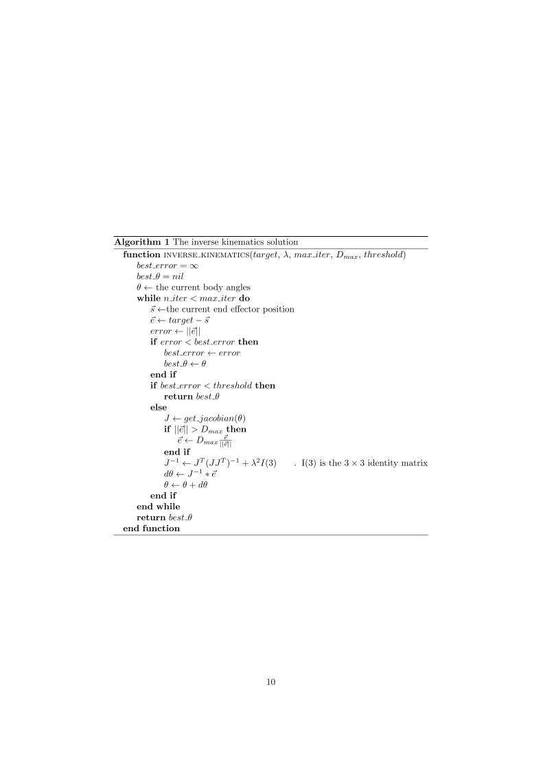
Algorithm 1 The inverse kinematics solution

function inverse kinematics(target, λ, max iter, Dmax, threshold)best error =∞best θ = nilθ ← the current body angleswhile n iter < max iter do

~s←the current end effector position~e← target− ~serror ← ||~e||if error < best error then

best error ← errorbest θ ← θ

end ifif best error < threshold then

return best θelse

J ← get jacobian(θ)if ||~e|| > Dmax then

~e← Dmax~e||~e||

end ifJ−1 ← JT (JJT )−1 + λ2I(3) . I(3) is the 3× 3 identity matrixdθ ← J−1 ∗ ~eθ ← θ + dθ

end ifend whilereturn best θ

end function

10

5.4.2 Contact point

The contact point is the point on the ball that has to be hit by the Nao to moveit in the desired direction. [10] uses the following calculation to find this, whichseems to work exactly as we would like:

~c− (~e ∗ r)

where ~c is the location of the center of mass of the ball, r is the ball radius (inthe case of the SPL balls this is 33.42 mm) and ~e is the force destination (thedirection of where we want the ball to end up in coordinates).

5.4.3 Retraction point

After the initial pose the Nao calculates its optimal retraction point. This isthe rearmost point from which the kick commences, and has two criteria thatshould be satisfied to be considered a good starting position:

• The retraction point should be far away from the ball (to make the kickas hard as possible)

• The retraction point should be accurate

To meet both criteria as good as possible there should be a trade off betweenthe two.

Firstly, to determine the point between the ball and a possible retractionpoint we use the following calculation:

dr = ~ex ∗ ||~px − ~pxc ||+ ~ey ∗ ||~py − ~pyc ||+ ||~pz − ~pzc || ∗ 0.3 (8)

Where ~pc is the contact point where the ball should be hit, ~p is a possibleretraction point, ~e is the unit vector pointing to the desired desination and ~drthe distance between both points. The importance of the x and y distancebetween the contact point and a possible retraction point relies on how much ofthe unit vector points to that direction. The z is held artificially high so thatthe leg will never be stretched to the ground.

Finding the accuracy of a given retraction point is less straightforward. Thisproblem can be seen as the closeness of a given point to the line, where the pointconsists of a possible retraction point and the line consits of the contact pointand the destination point. See Figure 4 for a visualisation of the problem. Thisidea makes for a basic linear algebra4 problem that needs to be resolved.

da =||(~pxy − ~pc

xy)× (~pxy − ~fdxy

)||‖ ~fd

xy− ~pc

xy‖

The distance to the line is only important in the xy direction, but a crossproduct can only be taken in 3D so this is solved by taking the xy values fromthe original points in space but adding a 0 value in the z direction. Now that wehave a way to calculate both the distance to the contact point and the accuracy

4The intuition behind this calculation can be found onhttp://mathworld.wolfram.com/Point-LineDistance3-Dimensional.html

11

~pc ~fd

da

~c

~p

Figure 4: Visualisation of the accuracy problem. the contact point (~pc) and the

preferable force direction ( ~fd) form a line in 3D space. A possible retraction point ~pcan be somewhere around this line. To find its accuracy the distance da should besolved. Note that this only concerns the x and y direction as the z dimension does notinfluence the accuracy. ~c denotes the center of mass location on the ball and is onlyshown for clarification.

towards the force direction, we are able to make a balanced decision towardswhat a good retraction point is.

~p = (1− δ) ∗ dr + δ ∗ 100

da(9)

We take the multiplicative inverse of da so that the value gets bigger whenthe retraction point is close to the line and rescale it by multiplying it with 100to make the value dr and da more in the same range. The value δ could beexperimented with to find the optimal result.Accuracy is more important thana big distance between ball and retraction point, something that will becomeevident in the results section.

All possible positions ~p should be considered to solve this equation. Todetermine what is possible the Nao is set in different positions and using aforward kinematics chain the end effector of each leg where the origin is thesupporting foot can be retrieved. This way roughly all possible positions are setand can be looped through to find the point that maximizes above equation.By also retrieving the location of the standing leg we make sure that there isno overlap in the reachable space and the position of the other leg.

6 Experiments and Results

6.1 Using force sensitive resistors for balancing

Since balancing in the y direction is the biggest challenge to stabilize we usedanother Nao to push the balancing Nao in this direction (see Figure 5). We ranthe script twice, one time with the balancer on and the second time where theoffsets of the angles where forced to 0 (keeping the plotting function but killingthe balance system)

12

Figure 5: Nao (right) pushing the other Nao (left) in the sideways (y) direction

Figure 6: With the balancer turned off (The Nao falls at 22 seconds)

13

Figure 7: With the balancer turned on (The Nao falls at 104 seconds)

As seen in the plots (Figure 6 and Figure 7), using the balancer helps to stayup longer (twice as long) but still can’t fully handle the external influences fromthe pushing Nao. The problem is that there aren’t many stable poses in thesideways direction and even a small change will have a relative large influenceon the sensor data. Due to this the sideways balancing tends to overshoot andthen start to oscillate. Taking a low Kp and Kd values gives a long settlingtime but minimizes the overshoot. The system now converges relative slow to astable position but is still able to negate external influences, providing a morestable and reliable balancer.

6.2 Inverse kinematics

Since our inverse kinematics solution relies on two parameters (λ and Dmax,see section 5.3), some testing needs to be done to optimize these. For testing,3 reasonable target positions were chosen, where the parameters were chosenfrom the set {λ,Dmax | λ ∈ (0.1, 0.25, 0.5, 1, 5), Dmax ∈ (10, 20, 30, 40, 50)}.The results can be seen in figures 8, 9 and 10. The error in the plots is definedas ||~t−~s||. Due to the large number of colored squiggly lines, each plot has beenrestricted to only parameter combinations which converged relatively quickly toaid in readability.

14

Figure 8: The first position, with the positional error set out against the time.

Figure 9: The second position, with the positional error set out against thetime.

15

Figure 10: The third position, with the positional error set out against the time.

In each case, the optimal value for λ was 5, while Dmax was either 50 or 20,which is a relatively large difference given the range of values. Of course, threetests isn’t enough to conclusively determine the optimal parameters, but theyoffer a nice starting point for further practical testing.

6.3 Calculating the retraction point

16

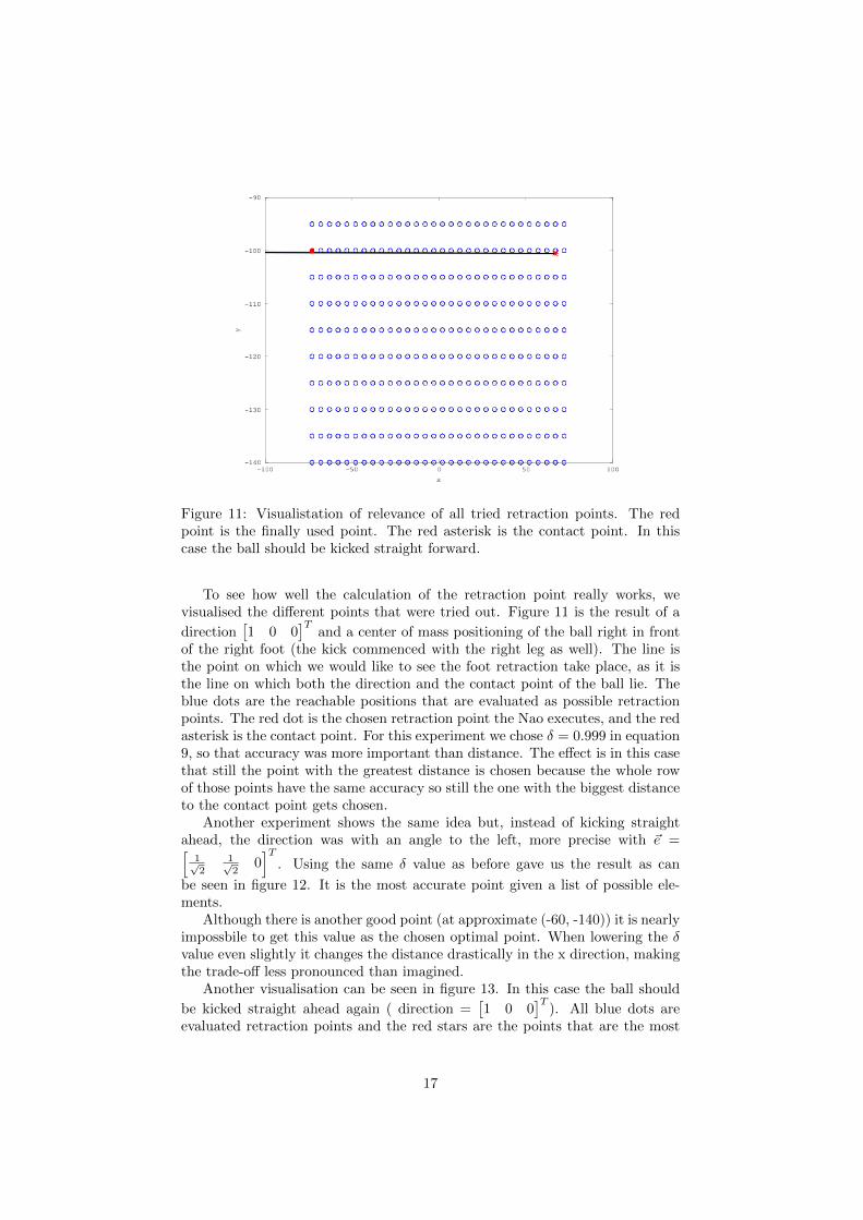
Figure 11: Visualistation of relevance of all tried retraction points. The redpoint is the finally used point. The red asterisk is the contact point. In thiscase the ball should be kicked straight forward.

To see how well the calculation of the retraction point really works, wevisualised the different points that were tried out. Figure 11 is the result of a

direction[1 0 0

]Tand a center of mass positioning of the ball right in front

of the right foot (the kick commenced with the right leg as well). The line isthe point on which we would like to see the foot retraction take place, as it isthe line on which both the direction and the contact point of the ball lie. Theblue dots are the reachable positions that are evaluated as possible retractionpoints. The red dot is the chosen retraction point the Nao executes, and the redasterisk is the contact point. For this experiment we chose δ = 0.999 in equation9, so that accuracy was more important than distance. The effect is in this casethat still the point with the greatest distance is chosen because the whole rowof those points have the same accuracy so still the one with the biggest distanceto the contact point gets chosen.

Another experiment shows the same idea but, instead of kicking straightahead, the direction was with an angle to the left, more precise with ~e =[

1√2

1√2

0]T

. Using the same δ value as before gave us the result as can

be seen in figure 12. It is the most accurate point given a list of possible ele-ments.

Although there is another good point (at approximate (-60, -140)) it is nearlyimpossbile to get this value as the chosen optimal point. When lowering the δvalue even slightly it changes the distance drastically in the x direction, makingthe trade-off less pronounced than imagined.

Another visualisation can be seen in figure 13. In this case the ball should

be kicked straight ahead again ( direction =[1 0 0

]T). All blue dots are

evaluated retraction points and the red stars are the points that are the most

17

Figure 12: Visualistation of relevance of all tried retraction points. The redpoint is the finally used point, the red asterisk is the contact point. In this casethe ball is kicked with an angle.

accurate(all have the same value). The data is set out over the xy axis, whichis the added length of the x and y direction, the z axis and the distance is thedistance as we measure it in 8 between contact point and the ball. The fact thatsometimes multiple of the same xy and z combinations have different distancesto the contact point is to be understood from the fact that although in the axisboth the real value of x and y are added to each other, equation 8 only considersthe value of x when the ball should go straight ahead.

18

Figure 13: Plot where the length of the xy direction between the contact pointand the retraction point are set out against the z direction and the distancefrom equation 8. The red points indicate the most accurate position

6.4 Integration of the Center of Mass balancers with thekick

Because of the limited ranges of both legs when it comes to reaching a ball wewould like the Nao to stand straight as much as possible while performing akick. When executing the initial pose we use the CoM balancer to seek themost balanced position, but it makes a lot of difference as to which joints in thesupport leg are used for balance. At first we experimented with the HipRoll andHipPitch to move to the most stable position. This however made for quite anunnatural pose, as you can see in Figure 14(a). Because executing a kick onlyuses the kicking leg, it can reach less of the relevant places.

Using the angle of the AnkleRoll and AnklePitch in the initial pose delivers amore natural position as seen in Figure 14(b), which makes it a better deicisionfor the initial pose.

7 Conclusion

Although the individual components mostly work as planned, integrating themall into an actual kick has proven harder than expected, which has left us unableto test the interactions between all of the components. For instance, using onlythe hip to compensate for balance is effective in the sense that it’s good atbalancing, but it results in poses where the kicking leg is unable to reach evennear the ground. Using the ankle however works just as well for balance, anddoesn’t suffer from the same problem. Unfortunately, there was no time forfurther testing in this regard.

Generation of the kick trajectory appears to work properly, although ithasn’t been thoroughly tested (only in a few directions) due to time contraints.Similarly, there is no data regarding the strength or stability of the kick, simplybecause there is no final kick yet.

19

The balancing system seems to work quite well and has been quite vigorouslytested. Still interferences from the side stay problematic, but only playing a realmath with the balancing turned on will show if it will work decent enough.

In the end, we’ve ended up with a nice motion framework which needs a bitmore work in order to have a completely functioning kick, which will hopefullyfunction as a basis for further motion-related tasks for the Dutch Nao Team(such as a new walking motion).

7.1 The retractionpoint

The above experimentations with finding a retractionpoint while making atrade-off between accuracy and distance seems to conclude that the retractioncalculation works as was expected for the basic cases. Due to time constraints,and the fact that less straightforward kicks are hard to visualise on a graphthere are still cases left out, but it already makes for a succesful kick in themost basic of situations.

8 Future works

Now that all subproblems of making a dynamic kick seem to be solved succes-fully, there are still some future improvements we would like to work on.

8.1 Wrapping up our current work

Firstly, we would like to integrate all elements talked about to make a succesfulkick. This was something we wanted to complete by the time this projectended, but in hindsight was a little too advanced for the limited timeframe.Nevertheless, we were still able to find solutions to every problem and can takeour time to combine both controllers and the kicking motion into a worthy finalresult.

8.2 Porting everything to C++

Many components were written in Python to aid in rapid prototyping, with helpfrom the Numpy module to allow for acceptable speeds. This works decently,but we unfortunately don’t have a way of running Numpy on our robots. Seeingas the Dutch Nao Team plans on switching to C++ for their codebase in thenear future, porting everything to C++ seems like the best option.

A Experimentations with solving the inverse kine-matics problem.

Before we arrived at our final inverse kinematics solution, we tried a numberof different (seemingly easier) options first. This section details some of theseexperimentations and why we have abandoned them.

20

A.1 Using built-in functions

The Naoqi framework running on the Nao robots offers a Cartesion ControlAPI 5 which contains a number of inverse kinematics function for setting andrequesting end effector locations in a specified coordinate system. The possiblecoordinate systems were “world” (where the origin was somewhere arbitrarilyaround the Nao), the torso and one between the legs. Because both the torsocoordinate system and the one between the legs are dependent of the postureof the Nao, we tried to work with the coordinate somewhere in space. Todetermine the range of the legs we took the Nao by hand and set the legs in themost stretched positions and retrieved the maximum and minimum x ,y and zvalues. These were taken as absolute ranges relative to a starting position. Inthe end this approach didn’t work as making a request for the current position aswell as setting a new position in this coordinate frame was not reliable enough.It seemed that the sensor values used to find these positions weren’t well enoughto use for such an operation. Another big problem is that actuation appearedto be quite slow; far too slow for a powerful football kick.

A.2 Using a simulator to find all reachable positions

We also tried to use the Cartesion Control API in a simulated environment6 toobtain a table containing all reachable locations of a given leg, within a certainresolution. Throughout a given range of world positions, the Nao was made tomove its foot there, after which the position of the foot was requested to see ifthe position had been reaches. In the end this was not as reliable as hoped dueto the same issues as spoken in the last section.

A.3 Making a lookup-table using Forward Kinematics

Because we already had a workable solution for forward kinematics, we thoughtabout creating a lookup table by iterating through a collection of joint angles andsaving them in a hashmap along with the corresponding end effector position.Integrating this using the balancing system however became a bit harder becausewe needed to track the position of the hip angles (these were, at the time usedfor changing the pose of the Nao) in the support leg, and in the end constructingthe inverse kinematics ourselves was an easier solution.

References

[1] JJ Alcaraz-Jimenez, M Missura, H Martinez-Barbera, and S Behnke. Lat-eral Disturbance Rejection for the Nao Robot. Proceedings of the 16thRoboCup Symposium, Mexico, June 2012, 2012.

[2] Samuel R Buss. Introduction to Inverse Kinematics with Jaco-bian Transpose , Pseudoinverse and Damped Least Squares methods.http://math.ucsd.edu/ sbuss/ResearchWeb/ikmethods/iksurvey.pdf, 2009.

5http://www.aldebaran-robotics.com/documentation/naoqi/motion/control-cartesian.html

6The environment used can be found on http://www.nao.sandern.com

21

[3] Dutch Nao Team. Dutch Nao Team - Team Description for Robocup 2012- Mexico City, Mexico. Technical report, 2012. to be published on theProceedings CD of the 16th RoboCup Symposium, Mexico, June 2012.

[4] Colin Graf, Alexander Hartl, Thomas Rofer, and Tim Laue. A RobustClosed-Loop Gait for the Standard Platform League Humanoid. Proceed-ings of the Fourth Workshop on Humanoid Soccer Robots in conjunctionwith the 2009 IEEE-RAS International Conference on Humanoid Robots,pages 30–37, 2009.

[5] Colin Graf and Thomas Rofer. A closed-loop 3D-LIPM gait for theRoboCup Standard Platform League humanoid. Fourth Workshop on Hu-manoid Soccer Robots in, 2010.

[6] Christiaan Meijer. Getting a kick out of humanoid robotics - Using rein-forcement learning to shape a soccer kick. Master’s thesis at the Universityof Amsterdam, 2012.

[7] Michael Meredith and Steve Maddock. Real-time inverse kine-matics: The return of the jacobian. Technical report, 2004.http://www.dcs.shef.ac.uk/intranet/research/resmes/CS0406.pdf.

[8] Judith Muller, Tim Laue, and Thomas Rofer. Kicking a Ball ModelingComplex Dynamic Motions for Humanoid Robots. RoboCup 2010: RobotSoccer World Cup XIV, pages 109–120, 2011.

[9] Johannes Strom and George Slavov. Omnidirectional walking using zmpand preview control for the nao humanoid robot. RoboCup 2009: RobotSoccer World Cup, pages 378–389, 2010.

[10] Yuan Xu and Heinrich Mellmann. Adaptive motion control: Dynamic kickfor a humanoid robot. KI 2010: Advances in Artificial Intelligence, pages392–399, 2010.

22

(a) Using the HipRoll and HipPitch tobalance the Nao

(b) Using the AnklePitch and An-kleRoll to balance the Nao

Figure 14: Experimentation with the influence of joint choice on the balancer

23