A Dissection of Trading Capital: Trade in the Aftermath of ...
35
A Dissection of Trading Capital: Trade in the Aftermath of the Fall of the Iron Curtain Matthias Beesterm¨ oller and Ferdinand Rauch *† This version: January 12, 2017 Abstract We study trade in Europe after the fall of the Iron Curtain, and show that the countries of the former Austro-Hungarian monarchy trade significantly more with one another after 1989 than predicted by a standard gravity model. This surplus trade declines linearly and monotonically over time. We suggest that the surplus comes from a mixture of increased trust, as well as better communication and information given Austria’s relationship with its eastern neighbors before the wars and during isolation. Trading capital, established under Habsburg rule and maintained in the period of the Iron Curtain, seems to have survived over four decades of separation and gives an initial boost to trade. This surplus trade disappeared rapidly after 1990 as countries rearranged themselves with the new geopolitical circumstances. We document the rate of decay of these forces. Keywords: Trade, Gravity, Habsburg Empire JEL codes: F14, F15, N33, N34, N94 * This paper has been improved by the comments and suggestions of numerous colleagues and seminar partic- ipants including but not limited to James Anderson, Franz Baltzarek, Felix Butschek, Daniel Baumgarten, Tibor Besedes, Johannes Van Biesebroeck, Felix Butschek, Mary Cox, Carsten Eckel, Peter Egger, P´ eter Es¨ o, Robert Evans, Thibault Fally, Gabriel Felbermayr, Lisandra Flach, Lionel Fontagn´ e, James Harrigan, Keith Head, Harald Heppner, Michael Irlacher, Beata Javorcik, Amid Khandelwaal, Helmut Konrad, Anna Koukal, Christopher Long, Thierry Mayer, Guy Michaels, Peter Neary, Volker Nitsch, Jana Osterkamp, Kevin O’Rourke, Chris Parsons, Steven Poelhekke, Monika Schnitzer, Jens S¨ udekum, Pierre-Louis Vezina, Daniel Wissmann as well as seminar and conference participants from the LETC conference in Slovenia, EGIT D¨ usseldorf, Paris, G¨ ottingen, ETSG Munich, Vienna and Zurich. We particularly thank two very helpful anonymous referees. Matthias Beesterm¨ oller gratefully acknowledges financial support from the DFG through GRK 1928 and the Egon-Sohmen-Foundation. † Affiliations: Rauch (corresponding author): Oxford University, [email protected]; Beesterm¨ oller: Ludwig-Maximilians-University of Munich, [email protected]. 1
Transcript of A Dissection of Trading Capital: Trade in the Aftermath of ...

A Dissection of Trading Capital:
Trade in the Aftermath of the Fall of the
Iron Curtain
Matthias Beestermoller and Ferdinand Rauch∗†
This version: January 12, 2017
Abstract
We study trade in Europe after the fall of the Iron Curtain, and show that the countries
of the former Austro-Hungarian monarchy trade significantly more with one another after
1989 than predicted by a standard gravity model. This surplus trade declines linearly and
monotonically over time. We suggest that the surplus comes from a mixture of increased
trust, as well as better communication and information given Austria’s relationship with
its eastern neighbors before the wars and during isolation. Trading capital, established
under Habsburg rule and maintained in the period of the Iron Curtain, seems to have
survived over four decades of separation and gives an initial boost to trade. This surplus
trade disappeared rapidly after 1990 as countries rearranged themselves with the new
geopolitical circumstances. We document the rate of decay of these forces.
Keywords: Trade, Gravity, Habsburg Empire
JEL codes: F14, F15, N33, N34, N94
∗This paper has been improved by the comments and suggestions of numerous colleagues and seminar partic-ipants including but not limited to James Anderson, Franz Baltzarek, Felix Butschek, Daniel Baumgarten,Tibor Besedes, Johannes Van Biesebroeck, Felix Butschek, Mary Cox, Carsten Eckel, Peter Egger, PeterEso, Robert Evans, Thibault Fally, Gabriel Felbermayr, Lisandra Flach, Lionel Fontagne, James Harrigan,Keith Head, Harald Heppner, Michael Irlacher, Beata Javorcik, Amid Khandelwaal, Helmut Konrad, AnnaKoukal, Christopher Long, Thierry Mayer, Guy Michaels, Peter Neary, Volker Nitsch, Jana Osterkamp,Kevin O’Rourke, Chris Parsons, Steven Poelhekke, Monika Schnitzer, Jens Sudekum, Pierre-Louis Vezina,Daniel Wissmann as well as seminar and conference participants from the LETC conference in Slovenia,EGIT Dusseldorf, Paris, Gottingen, ETSG Munich, Vienna and Zurich. We particularly thank two veryhelpful anonymous referees. Matthias Beestermoller gratefully acknowledges financial support from theDFG through GRK 1928 and the Egon-Sohmen-Foundation.
†Affiliations: Rauch (corresponding author): Oxford University, [email protected];Beestermoller: Ludwig-Maximilians-University of Munich, [email protected].
1

1 Introduction
In 1989 the Iron Curtain fell quickly and unexpectedly, ending the separation between Western
Europe and the Soviet Union. After 44 years of an almost completely sealed border, trade
was suddenly free to reconnect. Despite the political and economic turmoil within the Eastern
regimes, trade between West and East almost doubled within five years after 1990. By the year
2000 it had almost tripled. We study this trade in the aftermath of the collapse of the Soviet
Union. We pay special attention to Austria, a country that has engaged in trading opportunities
beyond what would be expected given its size and geographic location, and might have been
the main western beneficiary of Europe’s economic expansion eastwards.
In a standard gravity equation setting we document that Austria indeed trades more with
countries east of the Iron Curtain after 1990 than gravity would predict. However, we find that
this effect is only found for the members of the former Habsburg Empire1. It declines linearly
and monotonically, and in our preferred specification becomes statistically insignificant after
a decade while the predicted magnitude becomes zero after two decades. This trade surplus
is not visible for trade relationships between Austria and the other countries east of the Iron
Curtain once we additionally control for the Habsburg effect. The magnitude of the Habsburg
surplus trade in 1990 is very large, about four times the effect of a monetary union. We find
no similar surplus trade for other western countries with the East.
We argue that these results can best be explained by assuming a deterioration of specific com-
ponents of ‘trading capital’ built up during the Habsburg years and maintained throughout
the Cold War period. The 44 years of Iron Curtain division severed all formal and business
relationships, almost all trade between East and West, and made personal contacts difficult.
However, historical legacies and cultural linkages persist, facilitated by some low level economic
ties during the Cold War. The decline of this surplus after 1990 reflects the continued disso-
lution of trading capital and the build-up of trading capital with other countries in Western
Europe.
The term ‘trading capital’ is introduced by Head, Mayer and Ries (2010, from here on we refer
to this paper as HMR) who show that after independence former colonies continue to trade for a
long period with their colonizers, at a declining rate. They suggest that this observation might
point to the presence of trading capital that is built up during colonization, and deteriorates
1Throughout this paper we use the terms ‘Habsburg monarchy’, ‘Habsburg Empire’ and ‘Austro-Hungarianmonarchy’ interchangeably, knowing that Austro-Hungary is only valid since 1867. We usually refer to theEmpire in its extension shortly before World War I, as displayed in Figure 1. Former Habsburg membersinclude Austria, Bosnia and Herzegovina, Croatia, Czech Republic, Hungary, Italy, Poland, Romania, Serbia,Slovakia, Slovenia and the Ukraine to differing degrees as detailed in Table 2 and Figure 1.
2

after independence. Trading capital consists of various components, that we can divide into
three broad categories that facilitate trade: (i) physical capital, such as roads, railway lines or
pipelines that connect countries and directly facilitate trade through reduced bilateral trade
costs; (ii) capital relating to personal communication, direct human interaction and contacts
or trust built up in repeated games, such as provided in structures of multi-national firms,
joint ventures or by frequent personal contacts and trust won through repeated interaction;
and (iii) all other variables that facilitate trade, that are not based on personal interaction and
formal or physical structures. These include all notions of cultural familiarity, such as those
facilitated by cultural norms, language, history, consumers’ familiarity with products, trust
based on similarity and familiarity of people with each other. Category (iii) may include past
decisions on institutional design and standards as basic as which side of the road to drive on
or what type of electric plug design to adopt.
We argue that the declining surplus trade of Habsburg countries after 1989 is comparable to
the dissolving trading capital described by HMR, but given the history of Central Europe only
relates to that part of trading capital that was not isolated by the Iron Curtain, which are
mainly the elements described in point (iii). At the beginning of the century the Habsburg
monarchy was a politically and economically well integrated country. In the second half of
the century it was split into two parts that were strictly separated for 44 years by the Iron
Curtain. During the separation all formal institutions of the Empire ceased to exist as there
were several waves of drastic institutional changes especially east of the Iron Curtain. Personal
relationships were hard to maintain, and multinational firms connecting East and West as well
as other formal institutions were broken apart. Physical transport capital such as railway lines,
pipelines and roads – already badly damaged in WWII – were deliberately destroyed, or left to
deteriorate. At the same time institutions and norms converged both within the East and within
the West of the Iron Curtain into two distinct blocks. The historical circumstances thus offer
a natural experiment setting in which we can observe some components of trading capital only
between members of the former Habsburg Empire. In particular, any surplus trade observed
after 1989 will overwhelmingly include those parts of trading capital that relate to point (iii)
above. Comparing these effects to HMR we find that these forces explain a quantitatively large
part of trading capital, and that they deteriorate at a rate smaller than suggested for all trading
capital by HMR.
We add direct evidence for this hypothesis in five ways. First, we show that this surplus trade
appears for the Habsburg countries, but not for a number of placebo combinations between
western and eastern countries in Europe. We also verify that our main finding, the declining
surplus trade for Habsburg countries is highly robust to alternative empirical strategies. When
3

looking at product level, we see the effect mainly for homogeneous rather than heterogeneous
goods. We would expect this if countries follow a heuristic not based on economic rationale
alone, since homogeneous goods make substitution less costly. Forth, we see that the effect
is stronger for those goods that were traded in the Habsburg Monarchy. Fifth, we rule out a
number of possible alternative explanations. We present evidence that information, trust and
relationships are most likely to explain the findings.
Our paper adds to the literature showing that the degree to which such cultural forces influence
trade seems to be large (for example Algan et al. 2010, Disdier and Mayer 2007, and Michaels
and Zhi 2010), linkages between countries are highly persistent once built up and trade once
interrupted takes a long time to recover (Felbermayr and Groschl 2013, Nitsch and Wolf 2013).
There have been suggestions that culture matters more for trade than either institutions or
borders (Becker et al. 2014). Our paper also adds to a growing literature which emphasizes
the long persistent effects of borders, institutions and culture. For example Guiso et al. (2009)
establish the importance of trust and cultural similarity on economic exchange. Meanwhile, Eg-
ger and Lassmann (2013) and Melitz and Toubal (2012) document the importance of common
languages. However, it is difficult to distinguish between cultural similarity and ease of com-
munication. Cultural proximity is inherently difficult to measure. A number of recent studies
have thus used proxy measures for cultural proximity such as voting behavior in the Eurovision
Song Contest (Felbermayr and Toubal 2010) or the United Nations General Assembly (Dixon
and Moon 1993, Umana Dajud 2012). Lameli et al. (2013) show that the similarity of German
dialects is an important predictor of trade within Germany. We add to this literature by pro-
viding an example and new measure of both the resilience of such historic and cultural effects
on trade, as well as its decline.
Our paper’s methodology is related to Redding and Sturm (2008), who study the development
of towns in West Germany and use the fall of the Iron Curtain as a natural experiment. Nitsch
and Wolf (2013) document that it takes between 33 to 40 years to eliminate the impact of the
Iron Curtain on trade within Germany. Our paper mirrors Nitsch and Wolf (2013): While they
show that borders remain visible in trade statistics long after they have been abolished, we
demonstrate that borders take a long time to diminish trade when newly constructed. Djankov
and Freund (2002) document that Russian regions continued to trade with each other 60 per
cent more in the period from 1994 to 1996, which is broadly consistent with our findings. Other
studies that use a similar setting to our paper are Schulze and Wolf (2009) who examine trade
within the Habsburg monarchy in the late 19th century and find that borders that later emerge
become visible in price data long before the collapse of the Empire. Thom and Walsh (2002)
study the trade effect of Anglo-Irish monetary dissolution and find little effect on trade. Becker
4

et al. (2014) also present evidence on the importance of the Habsburg Empire on cultural norms.
When comparing individuals living east and west of the long-gone Habsburg border, they find
that people living on territory of the former Habsburg Monarchy have higher trust in courts and
police. They argue that the former Empire had an enduring effect on people’s values through
it’s decentralized, honest and widely accepted state bureaucracy.
Trade is only one of many possible measures that could be influenced by historical legacies
and cultural persistence. Migration and FDI might be others. Like HMR we choose to discuss
this effect in terms of trade given that trade is recorded in a more consistent way and at a
higher frequency than the aforementioned other measures. It is also less influenced by political
decisions. For example migration in Europe remained highly politically regulated until the EU
enlargement, and migration numbers are thus politically constrained.
This paper proceeds as follows: after a brief historical overview concerning the decline of the
Habsburg Empire, the Iron Curtain and the reunion of the continent as far as these events
concern our study in Section 2, we discuss our empirical strategy in Section 3. We then present
our estimates of the surplus trade and its decline among former Habsburg countries in Section 4
and Section 5, which focuses on product level results. Section 6 discusses the implications of the
trade boost and Section 7 concludes. The Appendix provides more details on the construction
of the dataset, and shows a few additional results and robustness tests.
2 Historical overview
In this paper, we take the borders of the Habsburg Empire as they were just before the outbreak
of World War I, displayed in Figure 1. While the Habsburg family had ruled the Empire for
many centuries with changing borders, unification attempts and the introduction of a centralized
administration came fairly late in the course of the 18th century.2 For our purposes, it is
important that the monarchy maintained a large, stable and well integrated market with large
internal trade flows throughout its last decades.
In 1913 the Austro-Hungarian Empire had a large degree of ethnic and linguistic diversity. All
parts of the monarchy were linked by a common official language, common legal institutions
2In the 13th century Rudolf von Habsburg acquired the thrones of Austria and Styria, which his family helduntil the first half of the 20th century. The Habsburg monarchy expanded over the centuries mainly throughskilful marriage policy, but also frequently lost territory in battle. The territory ruled by this family alwaysincorporated different languages, customs and religions, which especially in the early years were allowed toflourish locally. There was little superstructure until the reforms under Maria Theresia and Josef II. helpedby chancellors Kaunitz and Metternich in the course of the 18th.
5

Figure 1Austro-Hungarian Empire in 1910 and modern country boundaries
Source: Habsburg map is from Jeffreys (2007), and the modern country boundaries come fromEurostat (2013).
and administration, as well as an expanding rail network. A strong emphasis on free trade
strengthened the economic integration and trade flows within the country throughout the 19th
century (Good 1984). The monarchy possessed a fully integrated monetary union with full
control maintained by the Austro-Hungarian Bank in Vienna. Fiscal policy of the Empire was
run as a joint operation, with separate budgets in Austria and Hungary contributing to the
same common imperial expenditures and debt services (Eddie 1989).
The monarchy consisted of 53 million people, numbering 13 per cent of the total European
population and producing 10 per cent of Europe’s GDP. As these figures imply, the economic
condition of the Austro-Hungarian monarchy in its final decades prior to 1913 was poor in
comparison to other European countries.3 Before the collapse of the Empire, some internal
trade barriers became visible in price data at the end of the 19th century, and nationalism
3For example Schulze (2010) documents poor performance in terms of GDP per capita growth for the monarchybetween 1870 and 1913, and even uses the term ‘great depression’ to describe the situation in the westernhalf of the Empire in 1873.
6

was on the rise long before the collapse, contributing to it (Schulze and Wolf 2009 and 2012).
Yet these studies highlight that the Empire possessed a heavily integrated internal market
at the beginning of the 20th century regardless of these tendencies. The monarchy further
consisted of a well-functioning administration that unified the workings of many institutions
across the countries it governed. The importance of the attachment of people to the imperial
administration and its government, and the political, economic and cultural integration of its
parts is highlighted by Clark (2013)4 and Boyer (1989)5 among other historians.
The end of World War I brought about a number of declarations of independence, which
were sealed by the treaties of Saint Germain (1919) and Trianon (1920). New borders were
drawn and new countries appeared, following considerations of ethnicity, language and trade
networks. All the newly founded democracies on the territory of the former monarchy now
included large numbers of ethnic and linguistic minorities. The newly founded Republic of
Austria was left with 23 per cent of the population of the former monarchy. Trade between
countries of the former monarchy remained high in the 1920s. De Menil and Maurel (1994)
present some evidence for strong trade in the years 1924-26 among successor states of the former
monarchy, roughly of the magnitude of trade within the British Empire at that time. They
explain the persistence of trade pointing to common history, shared linguistic and cultural
ties, and mention the importance of business and personal relations as well as networks – all
parts of trading capital. Institutional drift, however, started. New and different currencies
were introduced. For example, Hungary replaced the Austro-Hungarian korona by its own
korona after independence only to replace it again by the pengo in 1925 and forint in 1946
following hyperinflation. The Austrian-Hungarian national railways was also split into multiple
corporations, though traffic across the former monarchy continued at a significant pace.
World War II disrupted trade substantially, and it did not recover in the aftermath. Beginning
in 1947, communist regimes in Central and Eastern Europe emerged under Soviet rule. The
Sovietization of these economies caused a breakdown of their trade relations with the West,
and foreign trade was organised as a strict state monopoly. Much of this remaining trade was
arranged from Moscow, and negotiated at the highest political level, often as part of political
4“[The administration] was an apparatus of repression, but a vibrant entity commanding strong attachments, abroker among manifold social, economic and cultural interests. [...] most inhabitants of the empire associatedthe Habsburg state with the benefits of orderly government: public education, welfare, sanitation, the ruleof law and the maintenance of a sophisticated infrastructure.”
5“ [...] competing popular and ethnic groups all had access to these public institutions [...] and these socialgroups quietly obtained some of their most sought after cultural attainments by means of these mechanisms,one might argue that the political and institutional history of the Empire presents [...] a state system thatwas not only more than the sum of its social parts, but was also psychologically consubstantial with thoseparts.”
7

bargains. An example for this was the export of goods worth 6.6 billion Austrian schillings in the
aftermath of its independence in 1955 to the Soviet Union (Resch 2010). Pogany (2010) writes
on the relationship between Austria and Hungary: ”Economic ties [...] became insignificant in
the years following World War II. Centuries-old relations were reduced to a minimal level [...].”
While Moscow took control of trade in the Eastern countries, on the western side trade was
also heavily politically influenced. The main driver of this was the Co-ordinating Committee
for Multilateral Export Controls (COCOM), established in 1949, an institution to organise
embargoes against Soviet countries. Austria did not formally become a COCOM member, but
its Eastern trade was influenced heavily by it under the obligations coming with Marshall aid
(Resch 2010). Economic cooperation was politically motivated and largely symbolic.
Large parts of infrastructure, especially the railways, were destroyed by the war - they would
only partially be rebuilt taking into account the new borders that had emerged. An anecdote
might highlight the poor recovery of infrastructure: The two capitals closest to each other in
Europe are Vienna and Bratislava, at a distance of less than 60 kilometers. During the time of
the monarchy there was a tramway that connected both cities, the “Pressburger Bahn”. There
has been no similar connection attempt since 1990, and thus the time to travel from one city
to the other is now larger than it was in 1900.6
The Iron Curtain was an ideological boundary, but also primarily a geographical border. The
most substantial cut to trade relations was brought about by the erection of the physical Iron
Curtain, whose construction begun in 1949. The new border ran right through the former
Habsburg countries, splitting Austria and the formerly Austrian parts of Italy from the rest.
After the Hungarian Uprising of 1956 the already very limited possibility of transit ceased and
all activity crossing this border was further suppressed. The border was sealed by barbed wire,
land mines, high voltage fences, self shot systems and other means. Only few people with
special permissions were allowed close to the border. As such the Iron Curtain thus presented
a completely sealed border that cut off all former local economic activity between the two sides
(Redding and Sturm 2008).
Furthermore, the economies of Hungary and Czechoslovakia switched to central planning.
Multinational companies were split, personal interaction and communication over the border
became increasingly difficult and rare. Table 1 shows the development of imports and exports
from Austria to former Habsburg countries, and Germany.7 The table shows a big decline of
both imports and exports between Austria and the other former Habsburg countries after 1920
6In the discussion of the results below we provide further examples of abandoned infrastructure between Eastand West.
7The numbers are from Butschek (2012), Tables 75 and 76.
8
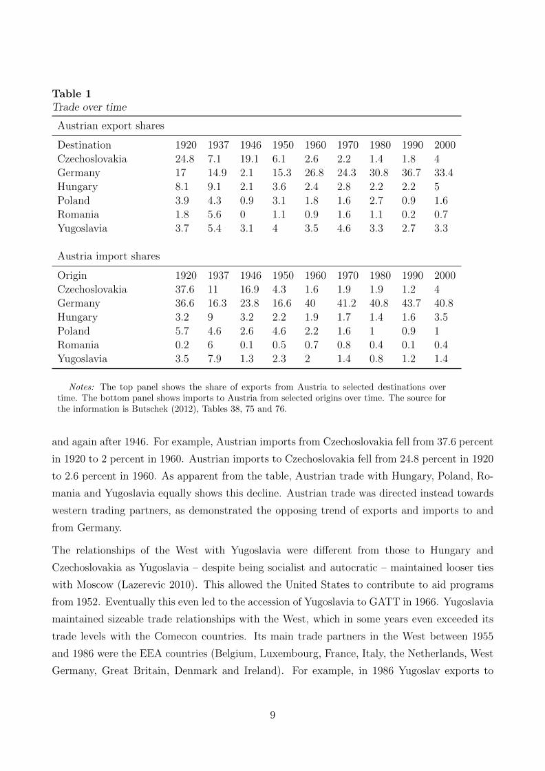
Table 1Trade over time
Austrian export shares
Destination 1920 1937 1946 1950 1960 1970 1980 1990 2000
Czechoslovakia 24.8 7.1 19.1 6.1 2.6 2.2 1.4 1.8 4
Germany 17 14.9 2.1 15.3 26.8 24.3 30.8 36.7 33.4
Hungary 8.1 9.1 2.1 3.6 2.4 2.8 2.2 2.2 5
Poland 3.9 4.3 0.9 3.1 1.8 1.6 2.7 0.9 1.6
Romania 1.8 5.6 0 1.1 0.9 1.6 1.1 0.2 0.7
Yugoslavia 3.7 5.4 3.1 4 3.5 4.6 3.3 2.7 3.3
Austria import shares
Origin 1920 1937 1946 1950 1960 1970 1980 1990 2000
Czechoslovakia 37.6 11 16.9 4.3 1.6 1.9 1.9 1.2 4
Germany 36.6 16.3 23.8 16.6 40 41.2 40.8 43.7 40.8
Hungary 3.2 9 3.2 2.2 1.9 1.7 1.4 1.6 3.5
Poland 5.7 4.6 2.6 4.6 2.2 1.6 1 0.9 1
Romania 0.2 6 0.1 0.5 0.7 0.8 0.4 0.1 0.4
Yugoslavia 3.5 7.9 1.3 2.3 2 1.4 0.8 1.2 1.4
Notes: The top panel shows the share of exports from Austria to selected destinations overtime. The bottom panel shows imports to Austria from selected origins over time. The source forthe information is Butschek (2012), Tables 38, 75 and 76.
and again after 1946. For example, Austrian imports from Czechoslovakia fell from 37.6 percent
in 1920 to 2 percent in 1960. Austrian imports to Czechoslovakia fell from 24.8 percent in 1920
to 2.6 percent in 1960. As apparent from the table, Austrian trade with Hungary, Poland, Ro-
mania and Yugoslavia equally shows this decline. Austrian trade was directed instead towards
western trading partners, as demonstrated the opposing trend of exports and imports to and
from Germany.
The relationships of the West with Yugoslavia were different from those to Hungary and
Czechoslovakia as Yugoslavia – despite being socialist and autocratic – maintained looser ties
with Moscow (Lazerevic 2010). This allowed the United States to contribute to aid programs
from 1952. Eventually this even led to the accession of Yugoslavia to GATT in 1966. Yugoslavia
maintained sizeable trade relationships with the West, which in some years even exceeded its
trade levels with the Comecon countries. Its main trade partners in the West between 1955
and 1986 were the EEA countries (Belgium, Luxembourg, France, Italy, the Netherlands, West
Germany, Great Britain, Denmark and Ireland). For example, in 1986 Yugoslav exports to
9

the EEA countries were over 7 times as large as exports to EFTA (Austria, Norway, Portugal,
Sweden and Switzerland) (Lazerevic 2010), which suggests that trade between Yugoslavia and
Austria was not particularly developed during the Cold War.
Table 2Habsburg Members
Country Share of land East Year of EU Year of Euro
that was Habsburg accession adoption
Austria 1 1995 1999
Bosnia and Herzegovina 1 1
Croatia 1 1 2013
Czech Republic 1 1 2004
Hungary 1 1 2004
Italy 0.05 1952 1999
Poland 0.12 1 2004
Romania 0.44 1 2007
Serbia 0.25 1
Slovakia 1 1 2004 2009
Slovenia 1 1 2004 2007
Ukraine 0.12 1
Notes: Share of land that was Habsburg denotes the share of the area of the modern country thatwas part of the Habsburg monarchy in the year 1910. The Habsburg dummy consists of countrieswith values of 1 in Column 1. Missing values in the last two columns indicate no membership in2013.
We mention only two properties of the fall of the Iron Curtain which are important here, namely
that it happened fast and that it was noted by almost everyone on either side of the border
with surprise (Redding and Sturm 2008).
These large changes of the map of Central Europe in the course of the 20th century are displayed
in Figure 1. The map displays modern country boundaries and a map of the Habsburg Empire
as of 1910. Table 2 shows the percentage of modern territory that was part of the Austro-
Hungarian Empire for modern countries. Most of the countries that were part of the Empire
are in the east, by which we indicate countries that were on the eastern side of the Iron
Curtain, to which we count the countries of former Yugoslavia. These countries are Bosnia
and Herzegovina, Croatia, the Czech Republic, Hungary, Slovakia, Slovenia as well as parts of
Poland, Romania, Serbia and the Ukraine. On the western side of the Iron Curtain we only
find Austria and South Tyrol, which is now part of Italy.
10

3 Empirical strategy and data
To investigate persistence after decades of Cold War of Austrian trade with countries east
of the Curtain (Austria-East8) and members of the former Habsburg monarchy, we largely
follow the methodology applied by HMR. They develop a method to address a closely related
question, and the similarity allows us to compare our estimates to theirs. We estimate gravity
equations, to which we add (Austria× East)× year and Habsburg × year dummies, which
are our principal variables of interest. We run the estimations once jointly with Austria-East
and Habsburg dummies, and once separately only including one set of dummies interacted with
year. We use the boundaries of the Habsburg Empire in its last days. The gravity framework
captures the counterfactual multinational trade had there been no Habsburg relationship. The
(Austria×East)× year and Habsburg × year indicators capture any trade in excess of what
the gravity model alone would predict.
The well-known empirical and theoretical formulations of the gravity equation can be repre-
sented in the following form:Xint = Cex
it Cimnt φint (1)
where Xint denotes importer n’s total expenditure on imports from origin i in year t, Cexit
and Cimnt are origin and destination attributes in a specific year, and φint measures bilateral
effects on trade.9 Since there is no set of parameters for which equation 1 will hold exactly,
the conventional approach is to add a stochastic term and estimate after log-linearizing. We
follow the commonly practiced gravity approach. Head and Mayer 2013 or Egger 2000 provide
overviews of this technique including a number of theoretical foundations which yield gravity
equations. In particular, we estimate the equation
ln(Xint) = µit + µnt + γDint + δ(Aus×East)(Aus× East)int + δHint + δeastHeastint + εint, (2)
where µit and µnt denote origin × year and destination × year fixed effects respectively and
δ coefficients to be estimated. The inclusion of sets of fixed effects interacted with year makes
separate time fixed effects as in equation 1 multicollinear and thus redundant. Matrix Dint
denotes pairwise covariates that may be time varying or not. In an effort to distill the main effect
of interest as precisely as possible, we include as detailed fixed effects as possible. In particular,
we include the variables shared border, common official and spoken language and common
legal institutions as time varying dummy variables to flexibly account for the many possible
changes in the cultural and political climate in Europe during this period. These sets of control
8A variable indicating a trade flow between Austria and a country east of the Iron Curtain9We follow HMRs notation here.
11

variables make it redundant to control for the standard right hand side variables measuring the
size of countries, such as population and income, and allow only to include bilateral variables
that vary over time. We include bilateral indicators for the distance between both countries,
indicators for a shared border, an officially joint language, a joint spoken language, common legal
institutions, common religion, common currency, the presence of a regional trade agreement as
well as indicators if both are members of the EU, the Euro zone, or on the east of the Iron
Curtain. All these standard bilateral control variables are taken from the standard source for
this type of estimation, and precise definitions are given there (Mayer and Zignago 2011). A
brief description of these measures is given in Appendix A.
The main variables of interest are the bilateral coefficients on the interaction term (Aus ×East)int, dummies indicating if the observed flow is between Austria and a country east of the
former Iron Curtain, and Hint, which indicates if both countries were once part of the Austro-
Hungarian monarchy in year t. Since we are only interested in Habsburg trade that crosses
the Iron Curtain, we also include a Heastint variable, which captures all trade east of the Curtain
(there is only Austria west of the Curtain in our baseline specification). Intuitively we estimate
how the fraction of Austria-East and Habsburg surplus trade evolves over time. We use a
comprehensive set of indicators to capture the different types of Habsburg trade. For our main
variable we restrict our measure of Habsburg economies to only those which were fully part of
the Habsburg monarchy: Austria, Hungary and former Czechoslovakia. We argue that this is
the safest approach as including other economies which were only partly part of the Empire,
such as Italy, may pick up effects not specific to the Habsburg relationship. In the appendix
we show robustness to different choices of this Habsburg definition.
If we were to control for attributes of the exporter and importer using GDP per capita and
populations our specification would suffer from bias caused by omission of “multilateral resis-
tance” terms (Anderson and van Wincoop 2003). Multilateral resistance terms are functions
of the entire set of φint from equation 1. We thus adopt the preferred method of the literature,
which is to introduce exporter-year and importer-year fixed effects.10 This full fixed effects
approach absorbs the exporting and importing specific effects.11 Exporter- and importer-year
fixed effects do not work for unbalanced two-way panels as pointed out by Baltagi (1995). If
actual bilateral data are not balanced, as is the case in HMR, one should use the least square
dummy variable (LSDV) approach. However, this concern is not relevant to our aggregated
European data set which is balanced.12 We therefore adopt the full fixed effects approach, even
10See Feenstra (2004) who addresses different techniques to take care of multilateral resistance within the gravityframework.
11See Egger (2000).12Appendix A lists our data sources and discusses our approach to minimize data inaccuracies.
12

though this approach has the disadvantage that we cannot observe the coefficients of some the
right-hand side variables typically used in gravity models.
We also address the issue of missing and zero trade observations. Zero and missing observations
may be due to mistakes or reporting thresholds, but bilateral trade can actually be zero. We
treat all missing trade observations as zero trade. Our linear-in logs specification of equation
2 removes all observations of zero trade, thus introducing a potential selection bias. In the
literature, it has been common to either drop the pairs with zero trade or estimate the model
using Xint = 1 for observations with Xint = 0 as the dependent variable.13 In our baseline
specification we choose to drop the zero pairs, but also run a robustness check replacing zeros
as ones. We also adopt the Poisson Pseudo-Maximum-Likelihood (PPML) estimation tech-
nique. A natural step would be to use Tobit which incorporates the zeros, but it assumes log
normality and homoskedasticity on the error term, so we prefer PPML. PPML incorporates
zeros and parameters can be estimated consistently with structural gravity as long as the data
are consistent, i.e. provided the expectation of ε conditional on the covariates equals one.14
The estimation method is consistent in the presence of heteroskedasticity.15 Thus, it provides
a natural way to deal with zero values of the dependent variable. We believe this preferable
to other estimators without further information on the heteroskedasticity. However, it may be
severely biased when large numbers of zeros are handled in this way (Martin and Pham 2009).
There are only 53 missing trade observations out of 13,200 observations in our data since we
focus on estimating trade among European economies. The majority of missing trade values
involve Albania as a trading partner for which trade may indeed be zero or so small that it falls
below a minimum reporting threshold.16
The estimation equation for the Poisson Pseudo-Maximum-Likelihood (PPML) estimator ex-
presses equation 2 as
Xint = exp(µit + µnt + γDint + δ(Aus×East)(Aus× East)int + δHint + δeastHeast
int
)uint, (3)
where uint = exp(εint).
Even though we include all the usual controls, our vector of bilateral variables may remain
incomplete, so unobserved linkages end up in the error term. To capture possible omitted
variables in εint, we estimate two additional econometric techniques: a lag dependent variable
13See, for example, Felbermayr and Kohler (2006).14See Silva and Tenreyro (2006).15Consistency of estimating equation 2 depends critically on the assumption that εint is statistically independent
of the explanatory variables.16See the Data Appendix for more details on the data set.
13

specification and a specification with origin-destination (bilateral or dyad) fixed effects. The
lagged dependent variable would absorb unobserved influences on trade that evolve gradually
over time. Including a lagged dependent variable biases coefficient estimates in short panel
models.17 Monte Carlo experiments suggest that the bias can be non-negligible with panel
lengths of T=10 or even T=15 (Dell et al. 2013). However, the time series dimension of our
panel (T=22) is likely long enough such that biases can be safely considered second-order.
Furthermore, the lagged dependent variable technique will not deliver consistent estimates if
there is a fixed component in the error term that is correlated with the control variables.
We thus also run a specification with bilateral fixed effects. We can still obtain estimates of
our coefficients of interest as our variation of interest is also varying over time (the Habsburg
and Austria-East dummies are interacted by year). The bilateral fixed effects specification
identifies the effect of Habsburg membership based on temporal (within-bilateral) variation. In
the bilateral fixed effects specification, all time invariant bilateral variables drop out.
To summarize, we estimate the Habsburg and Austria-East coefficients of interest using four
different estimation techniques closely following HMR: simple OLS, Poisson Pseudo Maximum
Likelihood (PPML), lag dependent variable specification and bilateral fixed effects (Dyad FE),
each with a strong set of fixed effects. Our typical estimation has in excess of 13,000 obser-
vations, and is robust to heteroskedasticity. We run these four estimations on the joint set of
Habsburg and Austria-East dummies and separately with one set of dummies interacted with
year. In the product level regressions we run the same specifications, but restrict the set of
products for which we run the regression in various ways. For example, we analyze homogeneous
and heterogeneous products separately to compare estimates.
The sources and details related to the construction of our dataset are documented in Appendix
A. All data we use and our treatment of them is standard throughout the related literature.
Here we just summarize a few decisions that we take. The dataset we use contains all European
countries in the years from 1990 until 2011, the first year for which Comtrade data is available
for all the countries of Europe after the fall of the Iron Curtain and the last year for which we
found a complete set of data when we embarked on this project. We clean Comtrade data using
the methodology of Feenstra et al. (2005). Trade data for the years before 1990 are available
from sources other than Comtrade, which we do not use given concerns about the comparability
of data. We use data for Europe only as we think that it provides a cleaner sample of countries
to run the proposed tests than the entire world would, given greater similarity of shipping and
other technology in Europe. The first OLS assumption that the correct model is specified is
easier to justify in a sample of more similar countries. We aggregate a few countries to maintain
17Nickell (1981) shows that the bias declines at rate 1T .
14

a balanced panel, see details of this in Table 1 in the Appendix. For the product regressions
we use the well known BACI dataset from CEPII, details described in Appendix A. CEPII
provided a BACI version that starts in 1992 for our countries, thus our product level analyses
begin only in 1993 throughout.
Figure 2Descriptive GDP and trade ratios(ratios on year)
Czechoslovakia
0
2
4
6
8
10
12
14
1990 1995 2000 2005 2010
GDP ratio: (GDPGER) / (GDPAUS)
Trade ratio to CZE: (XCZE,GER) / (XCZE,AUS)
Hungary
0
2
4
6
8
10
12
14
1990 1995 2000 2005 2010
GDP ratio: (GDPGER) / (GDPAUS)
Trade ratio to HUN: (XHUN,GER) / (XHUN,AUS)
Poland
0
2
4
6
8
10
12
14
1990 1995 2000 2005 2010
GDP ratio: (GDPGER) / (GDPAUS)
Trade ratio to POL: (XPOL,GER) / (XPOL,AUS)
Before turning to the regression results, we present some descriptive statistics which document
the Habsburg trading surplus relative to Germany.18 Figure 2 considers trade of Germany and
Austria with Czechoslovakia, Poland and Hungary. Czechoslovakia borders on both Germany
(both East and West) and Austria, thus differences in distance seem negligible. Moreover,
changes in multilateral resistance should also be fairly similar.19 We plot the ratio of German
18We later use Germany as a placebo as it shares the language with Austria, and also directly borders manyeastern countries. A risk of using that placebo might be that Germany could have also integrated faster withthe East for its own particular history. However, as Nitsch and Wolf (2013) observe, there was “remarkablepersistence in intra-German trade patterns along the former East-West border”.
19A surge in French or Spanish GDP would have similar effects on Germany and Austria.
15

to Austrian GDP(
GDPGt
GDPAt
)and the ratio of German trade with Czechoslovakia to Austrian
trade with Czechoslovakia(
XGer,Cze,t
XAus,Cze,t
). If Habsburg did not matter, we would expect the ratio
of trade to mirror the ratio of GDP (using GDP as measure for market and production size).
However, we observe a large gap. In 1990 the German economy is roughly ten times as large as
the Austrian economy. At the end of our sample period this ratio falls to about 8.5. However,
trade with Czechoslovakia is only three times as large for Germany and this ratio rises to just
over 6 over the sample period. We also conduct the same exercise for Hungary and Poland. On
the one hand, Hungary – yet another core Habsburg member – displays an even starker gap.
The trade ratio rises from approximately 2 to 4.5. These graphs highlight that Austria’s trade
with these two eastern countries was highly over-proportional given its size relative to Germany,
but that this surplus steadily lowered over time. Even Poland, which we do not regard as a
Habsburg member, since only 10 per cent of its mass belonged to the monarchy, and which does
not share a border with Austria, exported less than ten times its Austrian exports to Germany
in 1990. All the countries show the central empirical finding in this figure, a strong Austrian
trade surplus that weakens over time. We now turn to a more rigorous exploration of these
suggested observations.
4 Results
We run three sets of regressions. First, we restrict the sample to Habsburg countries. Second,
we include Austria-East dummies to investigate surplus trade with all of the East. Third, we
control for Austria-East and Habsburg jointly and find that the effect for Austria-East becomes
insignificant once we control for Habsburg. The first of these specifications is most important
for our conclusion. We present it in detail and focus on the main elements of the other two.20 It
is worth emphasizing that we use origin interacted with year fixed effects and destination times
year fixed effects separately in all of these regressions. The Habsburg surplus trade coefficients
are bilateral and vary annually by construction. Thus, they are not multicollinear with the
inclusion of this strong set of control variables and fixed effects.
In Table 4 we plot the Habsburg × year coefficients, which we interpret to be the surplus
trade of Habsburg countries relative to what we would expect if trade followed our gravity
model. These coefficients are also depicted in Figure 3. All four estimation methods display
a steady decrease of the Habsburg surplus trade over time. We confirm that the first and last
20Tables reporting coefficients of control variables and the exact Habsburg and Austria-East coefficients areomitted for length but available upon request.
16

estimated coefficients are statistically significantly different to each other.21 The downward
slope of the trend given in Figure 3 is strongly significant in all of the specifications, and the
slope is remarkably similar. It shows a strongly statistically significant, monotonic decline with
a slope of around -0.044. Thus the main results, namely that the cultural component of trading
capital declines over time, is insensitive to our estimation method. Note that the Habsburg
trade bonus is large in the first year after the collapse of the Iron Curtain. For example, in
the specification of column (1) the additional trade in the year 1990 is 0.69, which is about
three times as large as the trade bonus from two countries having a regional trade agreement
(0.24), two times as large as both countries having the same religion (0.34) and 1.6 times as
large as both countries being located in Eastern Europe. This magnitude also corresponds to
additional trade by a factor of e0.69, which is close to two. The surplus trade declines steadily
and becomes statistically insignificant about ten years after the fall of the Iron Curtain. Note
that the coefficients with Habsburg alone show stronger effects, smaller margins of error, and
are more precisely estimated than the Austria-East coefficients.
Figure 4 displays the Austria-East by year interaction terms from an estimation with Austria-
East coefficients. These results show a statistically significant effect in 1990 which declines
linearly and monotonically in both OLS and PPML estimation techniques. The other two tech-
niques show no significant results. Once we add controls for the Habsburg × year coefficients,
this trend becomes insignificant in our preferred specification. A weak downward slope re-
mains only in the PPML specification, statistically insignificant from zero, see Figure 5. These
graphs suggest that Austria-East does not play a pronounced role once we control for Habsburg
membership.
In Table 3 we proceed to estimate equations 2 and 3 from above with only coefficients for
Habsburg membership. As expected, distance negatively impacts trade in all specifications
where we can include this control variable. The displayed time varying dyadic effects tend
to show the expected sign, but coefficients vary across specifications. The latter is expected,
as these specifications differ in many respects, for example the PPML code is written to be
estimated using levels rather than natural logarithms on the left hand side variable. Silva and
Tenreyro (2006) also find a significantly smaller effect of geographical distance. Some of the
coefficients show unexpected signs, such as negative coefficients for common currency and “Both
EU”. This might reflect that some wealthy economies such as Norway and Switzerland are not
part of EU and Eurozone. The PPML coefficient of distance exactly corresponds with that of
HMR.
21F-test Probability > F values are OLS: .008; PPML: .001; Lag DV: .768; and Dyad FE: .000.
17

Table 3Estimation with Habsburg - year fixed effects onlyCoefficients of control variables
(1) (2) (3) (4)OLS PPML Lag DV Bilateral FE
Dependent variable: ln(xint) xint ln(xint) ln(xint)
Variable of interest:Habsburg - year fixed effects – Coefficients are reported in Table 4 and Figure 3 –
Time fixed dyadic effects:Log distance -1.181*** -0.641*** -0.213***
(0.0239) (0.0113) (0.0215)Common religion 0.344*** 0.108*** 0.0614***
(0.0336) (0.108) (0.0162)Both East 0.419*** 0.116*** -0.0358
(0.0491) (0.0455) (0.0304)Shared border - year Yes Yes Yes YesOfficial common language - year Yes Yes Yes YesCommon language spoken - year Yes Yes Yes YesCommon legal institutions - year Yes Yes Yes Yes
Time varying dyadic effects:Common currency -0.197*** 0.00541 -0.00482 -0.0192
(0.0358) (0.0339) (0.0188) (0.0307)Regional trade agreement 0.237*** 0.288*** 0.0576 0.344***
(0.0560) (0.0531) (0.0411) (0.0570)Both EU -0.0119 -0.108*** 0.0175 -0.00553
(0.0396) (0.0319) (0.0198) (0.0222)Both Euro -0.0862*** 0.271*** -0.0451*** -0.0302
(0.0280) (0.0311) (0.0157) (0.0363)Lagged exports 0.831***
(0.0126)
Origin country - year fixed effects Yes Yes Yes YesDestination country - year fixed effects Yes Yes Yes YesBilateral fixed effects No No No YesHabsburg - east - year fixed effects Yes Yes Yes Yes
Observations 13,147 13,200 12,518 13,147R-squared 0.937 0.966 0.982 0.976
Notes: This Table and Table 4 display different coefficients from the sameregressions. Columns 1, 2 and 4 provide estimates of equation 2, Column 2 fromequation 3. Table 4 shows the Habsburg × year coefficients. These coefficientsare depicted in Figure 3. Stars denote statistical significance on the level of one(***), five (**) and ten (*) per cent. Robust standard errors used.
18
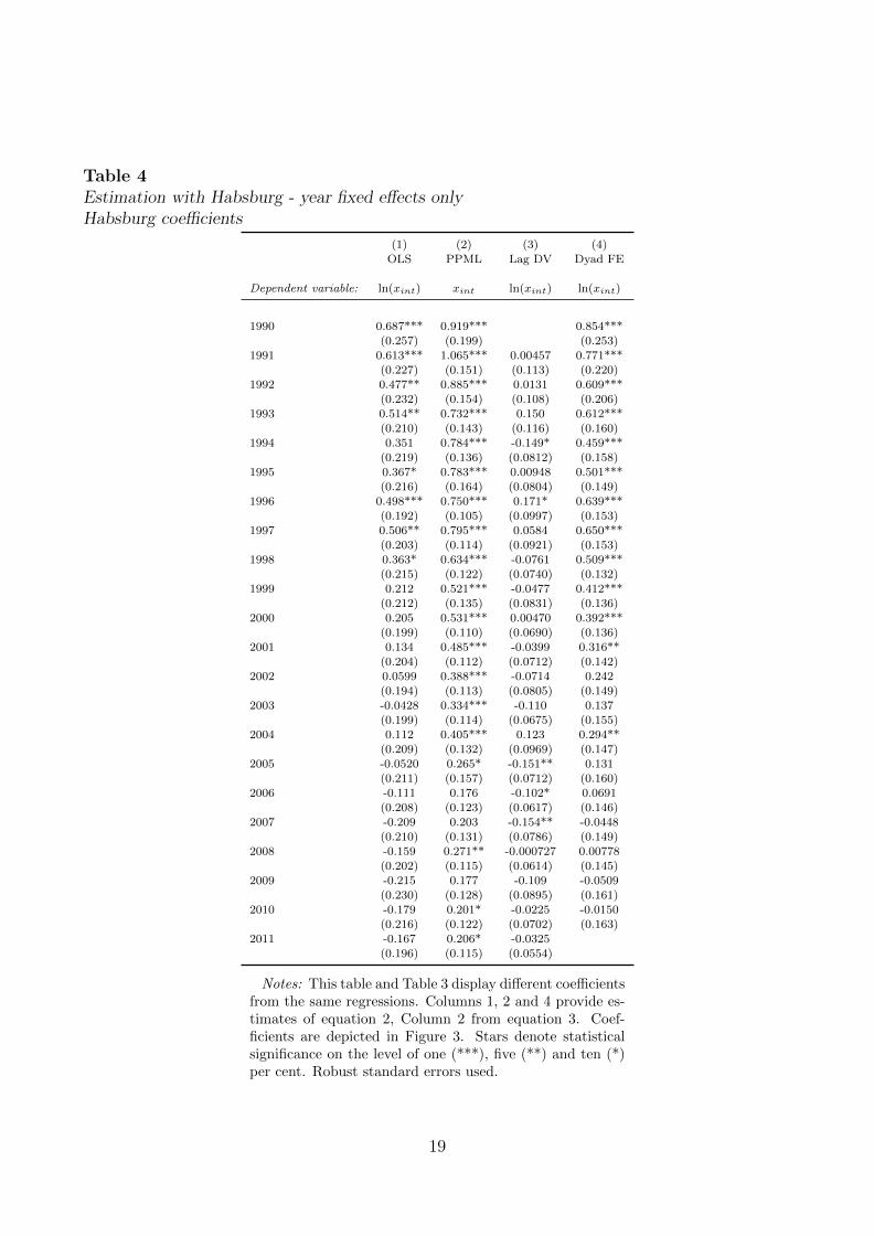
Table 4Estimation with Habsburg - year fixed effects onlyHabsburg coefficients
(1) (2) (3) (4)OLS PPML Lag DV Dyad FE
Dependent variable: ln(xint) xint ln(xint) ln(xint)
1990 0.687*** 0.919*** 0.854***(0.257) (0.199) (0.253)
1991 0.613*** 1.065*** 0.00457 0.771***(0.227) (0.151) (0.113) (0.220)
1992 0.477** 0.885*** 0.0131 0.609***(0.232) (0.154) (0.108) (0.206)
1993 0.514** 0.732*** 0.150 0.612***(0.210) (0.143) (0.116) (0.160)
1994 0.351 0.784*** -0.149* 0.459***(0.219) (0.136) (0.0812) (0.158)
1995 0.367* 0.783*** 0.00948 0.501***(0.216) (0.164) (0.0804) (0.149)
1996 0.498*** 0.750*** 0.171* 0.639***(0.192) (0.105) (0.0997) (0.153)
1997 0.506** 0.795*** 0.0584 0.650***(0.203) (0.114) (0.0921) (0.153)
1998 0.363* 0.634*** -0.0761 0.509***(0.215) (0.122) (0.0740) (0.132)
1999 0.212 0.521*** -0.0477 0.412***(0.212) (0.135) (0.0831) (0.136)
2000 0.205 0.531*** 0.00470 0.392***(0.199) (0.110) (0.0690) (0.136)
2001 0.134 0.485*** -0.0399 0.316**(0.204) (0.112) (0.0712) (0.142)
2002 0.0599 0.388*** -0.0714 0.242(0.194) (0.113) (0.0805) (0.149)
2003 -0.0428 0.334*** -0.110 0.137(0.199) (0.114) (0.0675) (0.155)
2004 0.112 0.405*** 0.123 0.294**(0.209) (0.132) (0.0969) (0.147)
2005 -0.0520 0.265* -0.151** 0.131(0.211) (0.157) (0.0712) (0.160)
2006 -0.111 0.176 -0.102* 0.0691(0.208) (0.123) (0.0617) (0.146)
2007 -0.209 0.203 -0.154** -0.0448(0.210) (0.131) (0.0786) (0.149)
2008 -0.159 0.271** -0.000727 0.00778(0.202) (0.115) (0.0614) (0.145)
2009 -0.215 0.177 -0.109 -0.0509(0.230) (0.128) (0.0895) (0.161)
2010 -0.179 0.201* -0.0225 -0.0150(0.216) (0.122) (0.0702) (0.163)
2011 -0.167 0.206* -0.0325(0.196) (0.115) (0.0554)
Notes: This table and Table 3 display different coefficientsfrom the same regressions. Columns 1, 2 and 4 provide es-timates of equation 2, Column 2 from equation 3. Coef-ficients are depicted in Figure 3. Stars denote statisticalsignificance on the level of one (***), five (**) and ten (*)per cent. Robust standard errors used.
19

Figure 3Estimation with Habsburg - year fixed effects onlyHabsburg coefficient plots
(1) OLSSlope: -.044 (.003)
-.5
0
.5
1
1.5
1990 1995 2000 2005 2010
(2) PPMLSlope: -.042 (.003)
0
.5
1
1.5
1990 1995 2000 2005 2010
(3) Lag DVSlope: -.006 (.003)
-.4
-.2
0
.2
.4
1990 1995 2000 2005 2010
(4) Dyad FESlope: -.043 (.003)
-.5
0
.5
1
1.5
1990 1995 2000 2005 2010
Notes: Coefficients of the Habsburg by year interaction term Hint in equation 2 and equation3 with 95 per cent confidence intervals. Line of best fit with slope and s.e. are also recorded.Restricted sample: includes only countries that were fully part of the Habsburg monarchy:Austria, Hungary and former Czechoslovakia. Coefficients of control variables are reported inTable 4.
One concern about these results might be that the opening of the trade relations between East
and West might be dynamic, increasing or decreasing, in the first years after the opening of the
Iron Curtain because of various reasons other than the decline of historic and cultural ties. For
example, the installation or reuse of transport infrastructure might suggest a dynamic trade
relationship between an eastern and a western country, or the slow establishment of personal
exchange and interaction. In both these examples we would expect an increasing relationship,
but there may be others. To mitigate concerns that such effects drive our results we run a
placebo exercise in which we estimate “Habsburg” effects on a relationship other than Habsburg,
for which we do not expect the same decay of cultural ties. We choose Germany as the placebo
country, which shares the language with Austria, and also a direct border with many eastern
20

Figure 4Estimation with Austria-East - year fixed effects onlyAustria-East coefficient plots
(1) OLSSlope: -.01 (.003)
0
.4
.8
1.2
1990 1995 2000 2005 2010
(2) PPMLSlope: -.027 (.002)
0
.5
1
1.5
1990 1995 2000 2005 2010
(3) Lag DVSlope: -.001 (.003)
-.2
0
.2
.4
.6
1990 1995 2000 2005 2010
(4) Dyad FESlope: -.008 (.003)
-.5
0
.5
1990 1995 2000 2005 2010
Notes: Coefficients of the (Aus× East)× year interaction term in equation 2 and equation 3with 95 per cent confidence intervals. Line of best fit with slope and s.e. are also recorded.
countries. When we estimate the trading relationship with Germany instead of Austria being
the “Habsburg” country west of the curtain, we do not find significant relationships. These
results are reported in Appendix B, and in this table we use the same specification as applied
in Tables 3 and 4. We also report results for similar placebo exercises using Switzerland, the
Netherlands, Belgium-Luxembourg and Italy as alternative placebo countries, and we find no
strong trend for either of these countries, with the exception of a moderate decrease in Italy,
which was partly Habsburg. We interpret this finding to cast doubt on the relevance of other
dynamic effects shaping initial trade relationships.
The appendix demonstrates robustness of these results for different estimation strategies, addi-
tional control variables, different choices for the Habsburg definition, aggregation of countries,
how to deal with missing and zero data, adding internal trade flows, and different treatment of
21

Figure 5Joint estimation with Austria-East dummies and Habsburg - year fixed effectsAustria-East coefficient plots
(1) OLSSlope: .002 (.004)
-1
0
1
1990 1995 2000 2005 2010
(2) PPMLSlope: -.01 (.003)
0
.5
1
1.5
1990 1995 2000 2005 2010
(3) Lag DVSlope: 0 (.004)
-.5
0
.5
1990 1995 2000 2005 2010
(4) Dyad FESlope: .004 (.004)
-.5
0
.5
1990 1995 2000 2005 2010
Notes: Coefficients of the (Aus× East)int interaction term in equation 2 and equation 3 with95 per cent confidence intervals. Line of best fit with slope and s.e. are also recorded.
standard errors. We find generally that this main trend is strongly robust to modifications of
this type.
5 Product level results
In this section we shed more light on the mechanism driving our main result by studying various
product categories separately. In Figure 6 we report the main OLS specification for each of the
two-digit HS product codes except for services for which no BACI data are available. In 13 of
the 15 plots the trend is downward sloping, and in 10 the downward trend is significant at 5%
level of significance. The graph is upward sloping for animal products and skins and leather,
both of which are small industries, accounting for 0.7 and 0.6 percent of all exports in Europe in
22

2000 respectively. This graph shows that our main results of a strong initial Habsburg surplus
that weakens over time is not driven by a few industries, but is observable for most industry
groups individually, to a varying degree however. The strongest effects in magnitude are found
for machinery, foodstuff and miscellaneous. The general trend within most groups implies that
industry composition changes alone cannot account for the observation of that effect.
If our results are driven by an instinct of going back to where things had been before the
wars, we might expect some correlation across industries from the monarchy to trade in the
1990s. We next run our main regression separately for products traded predominantly in the
monarchy and other products. Given changing boundaries, and changes in the product space
this can only be done on a broad level, and remains an exercise with noise. Eddie (1989)
characterises the dual monarchy as a marriage of wheat and textiles. Good (1984) lists as main
traded items in the monarchy from 1884 to 1913 food and beverages, crops, sugar, flourcrops,
sugar and flour originating in Hungary and industrial raw materials, textiles, machinery, and
manufactured products originating in Austria. Following these classifications we classify the
industries foodstuff, machinery, and textiles as main industries traded in the monarchy. We
find that both product classes show a significant, monotonic downward slope, which is not
surprising given that we find the downward slope for most individual HS2 product categories.
The initial trade bonus for the Habsburg traded goods is almost double that for the others, and
the slope in the plot showing the Habsburg traded goods is also 2.8 times larger. The trade
surplus becomes insignificant in both cases in the 2000s.
23

Product: 1 -- 5Slope: .021 (.013)
-1.5
-1
-.5
0
.5
1
1.5
1990 1995 2000 2005 2010
Product: 6 -- 15Slope: -.012 (.009)
-1.5
-1
-.5
0
.5
1
1.5
1990 1995 2000 2005 2010
Product: 16 -- 24Slope: -.047 (.008)
-1.5
-1
-.5
0
.5
1
1.5
1990 1995 2000 2005 2010
Product: 25 -- 27Slope: -.009 (.008)
-1.5
-1
-.5
0
.5
1
1.5
1990 1995 2000 2005 2010
Product: 28 -- 38Slope: -.016 (.004)
-1.5
-1
-.5
0
.5
1
1.5
1990 1995 2000 2005 2010
Product: 39 -- 40Slope: -.023 (.007)
-1.5
-1
-.5
0
.5
1
1.5
1990 1995 2000 2005 2010
Product: 41 -- 43Slope: .021 (.016)
-1.5
-1
-.5
0
.5
1
1.5
1990 1995 2000 2005 2010
Product: 44 -- 49Slope: -.01 (.006)
-1.5
-1
-.5
0
.5
1
1.5
1990 1995 2000 2005 2010
Product: 50 -- 63Slope: -.014 (.004)
-1.5
-1
-.5
0
.5
1
1.5
1990 1995 2000 2005 2010
Product: 64 -- 67Slope: -.007 (.006)
-1.5
-1
-.5
0
.5
1
1.5
1990 1995 2000 2005 2010
Product: 68 -- 71Slope: -.017 (.007)
-1.5
-1
-.5
0
.5
1
1.5
1990 1995 2000 2005 2010
Product: 72 -- 83Slope: -.034 (.006)
-1.5
-1
-.5
0
.5
1
1.5
1990 1995 2000 2005 2010
Product: 84 -- 85Slope: -.075 (.007)
-1.5
-1
-.5
0
.5
1
1.5
1990 1995 2000 2005 2010
Product: 86 -- 89Slope: -.026 (.008)
-1.5
-1
-.5
0
.5
1
1.5
1990 1995 2000 2005 2010
Product: 90 -- 97Slope: -.035 (.005)
-1.5
-1
-.5
0
.5
1
1.5
1990 1995 2000 2005 2010
Figure 6Main specification by HS2 product groups, in increasing numerical score: animal prods (1-5), vegetable prods (6-15), foodstuff(16-24), mineral prods (25-27), chemical industries (28-38), plastics (39-40), skins and leather (41-43), wood prods (44-49), textiles(50-63), footwear (64-67), stone and glass (68-71), metals (72-83), machinery (84-85), transportation (86-89), miscellaneous (90-97).
24

We next study the effect by heterogeneous and homogeneous products, following the standard
classification by Rauch (1999). We merge the classification at the level of HS4, keeping only
matched trade flows. These are fifteen per cent of total trade flows. We think that the Habsburg
bonus disappears over time as Europe adjusts to the new trading environment, and converges to
the new optimum. This suggests that initial deviations from the optimum, which here happen
to coincide with the gravity framework, were not the first best choice. We would expect to find
that the Habsburg bonuses are thus stronger for homogeneous goods, for which search costs
and the costs of not using the optimum product are smaller, and thus the temptation to follow
an intuitive heuristic when buying greater. As can be seen in the top panels of Figure 7, indeed
we find the bonus is stronger initially, and falls more rapidly for the homogeneous goods, while
there is not such a clear pattern for the differentiated products.
Figure 7By degree of heterogeneity and transport costs.
differentiatedSlope: -.011 (.009)
-1.5
-1
-.5
0
.5
1
1.5
1990 1995 2000 2005 2010
homogenousSlope: -.053 (.006)
-1.5
-1
-.5
0
.5
1
1.5
1990 1995 2000 2005 2010
costlySlope: -.025 (.004)
-1.5
-1
-.5
0
.5
1
1.5
1990 1995 2000 2005 2010
cheapSlope: -.051 (.004)
-1.5
-1
-.5
0
.5
1
1.5
1990 1995 2000 2005 2010
Notes: Coefficients of the Habsburg by year interaction term Hint in equation 2 and equation 3with 95 per cent confidence intervals. The top two panels compare trade of differentiated andhomogeneous goods. The bottom two panels consider the different transport costs.
25

If transport infrastructure surviving from the monarchy was an important driver of our findings,
we should expect to see a stronger effect for goods easier to transport. To measure this effect
we obtain data on unit values from the CEPII TUV dataset. This dataset gives Free on Board
(FoB) unit values per ton for each HS6 product. If, in line with some literature, we assume
that the costs to ship a ton of any good are fairly similar, then inverse unit value data can
serve as a proxy for transport costs, as the ratio of transport costs per value transported would
be smaller. Using this proxy we compare above and below median goods separately, in the
bottom two panels of Figure 7. The panel of ‘costly’ goods refers to above median transport
cost goods, while ‘cheap’ refers to below median ones. The standard pattern emerges, and
the initial surplus trade is similar in both specifications. If there was a difference, it would be
that the goods that are harder to transport adjust earlier. An explanation for this earlier drop
may be that for these goods the costs of a suboptimal country to import from are higher, so
adjustment may be quicker. In any case, this difference is not very strong, and coefficients rest
firmly within the confidence intervals of the other graph in both cases.
6 Discussion
We consider a number of possible explanations why the countries of the monarchy trade more
with each other in the first years after the collapse of the Iron Curtain, and why this initial
trade bonus declines over time. First we rule out a number of explanations we consider less
likely, before presenting explanations we find more plausible.
6.1 Less plausible explanations
First, this result might just be a consequence of a miss-specification of the gravity equation.
A highly structural approach of the kind we employ is easily prone to introduce noise when
looking at specific bilateral trade volumes. If, for example, we overestimate the distance between
Austria and the eastern countries, the residuals for these bilateral observations in a standard
gravity model would be positive.22 Or there might be some natural geographic advantage that
facilitates trade between these countries, and this reason might have brought about both the
Monarchy before 1918 and the surplus trade after 1989. Explanations and examples of this type
could cast doubt on the existence of a static Habsburg surplus trade. What we observe is a
trade bonus that declines linearly and monotonically over time, and it does so robustly across a
22Given the location of Vienna in the east of Austria we actually underestimate the distance relative to theharmonic mean suggested in Rauch (2016).
26

number of very different estimation methods. This dynamic result is hard to explain as a simple
statistical property of miss-specification or measurement error. If it was a purely mechanical
specification error, our placebo exercise, that replaces Austria with Germany, would be prone
to suffer from the same problem, and show the same downward slope. We verify that our main
specification is robust to the use of different measures of distance, such as the distance between
the most populated city, and two measures of weighted distances. Our numerous robustness
checks which vary estimation strategy, aggregation of countries and control variables should
also help to address this concern.
Second, this surplus trade may stem from better existing transport infrastructure dating back
to the times of the monarchy. However, most of this infrastructure was unused and laid bare
during the Cold War and by 1989 was derelict. The main rail lines connecting Austria with
the East were abandoned; for example in 1945 the track connecting Bratislava and Vienna, the
Pressburger Bahn, the rail to the Czech Republic via Laa an der Thaya and the connection
via Fratres-Slavonice were abandoned. All these lines were not revived until today. Transcon-
tinental connections such as Vienna-Hamburg or Vienna-Berlin have switched permanently to
run via Passau instead of Prague. There is also evidence that reconstruction and construction
of new networks was slow after 1990, as in Hungary “there were no significant changes in the
lengths of the linear transport network in the first half of the 1990s” (Erdosi 1999). Further,
even if a derelict rail line provides a strong advantage to trade, we would not expect this surplus
to contribute immediately given the time it takes to renovate such a network. Thus we would
expect a rise of the Habsburg bonus in the first years, as infrastructure is slowly brought back
to full capacity. In the product level section we do not find a big difference between products
that are cheap or expensive to transport, which should also address this concern.
Third, this trade bonus might just reflect the specific history of bilateral developments after
1989 that are unconnected to prior history. Austria might have had a starting advantage, after
all it was between Austria and Hungary that the Iron Curtain first opened. While it is true that
the Iron Curtain was symbolically opened first between Austria and Hungary, things moved
rapidly after that. The first symbolic opening on August 19th 1989 was less than three months
before the opening of borders within Germany on November 9th. The first time Germans could
flee was on September 10th and 11th. Most of the people who fled in the two months before the
broader opening were East Germans. Thus, the head start was neither long, nor specifically
beneficial to the Austrian economy.
Fourth, it may be that language barriers have initially favored trade from Austria to the East,
given that a higher fraction of citizens in the eastern countries still speak German than in other
27

European countries. This explanation is similar to the interpretation we favour, however the
placebo exercise using Germany and Switzerland suggest that the German language cannot
explain this surplus trade, and in fact does not seem to contribute to its decline.
Fifth, political factors such as Austria’s neutrality may have helped to win the trust of eastern
trading partners. This however should predict a general increase in trade for Austria with all
eastern countries, rather than the selected members of the former monarchy, and would be
absorbed by the interactions of Austria with all of Eastern Europe that we include. Further,
we would not expect this or similar effects to decline over time as Austria’s political neutrality
persists.23 The placebo exercise using neutral Switzerland may also help to address this con-
cern. As Butschek (2011) notes, the Austrian government contributed little to build friendly
relationships with its eastern neighbors in the first years after 1990.
6.2 More plausible explanations
Butschek’s economic history of Austria (2011) discusses the relationship between Austria and
the former Habsburg countries in the East in the 20th century. He describes the trade patterns
studied in this paper: strong economic ties during the monarchy, the strong trade links in
the inter-war period, drastic stagnation of trade in the period of the Iron Curtain, a trade
boom in the 1990s. He names Austria the greatest Western beneficiary from the economic
expansion towards the East. Butschek explicitly states that historic factors likely explain the
trade surplus after 1990. He also notes geographic proximity, and suggests that Austria may
have an informational advantage over other Western countries. He points out that the trade
boom happened without help from the Austrian government, in fact the Austrian government
slowed it through aggressive diplomacy towards the East in the 1990s.
Butschek’s key explanation for the surplus trade is given on page 405: “Austrian managers
seem to have been more familiar with the situation in the successor states than their colleagues
from other countries.”24 Here, we translate the original verb “vertraut sein” as “familiar with”.
However, it’s German form offers a wider meaning: “vertrauen” also means “to trust”, and
when used as a noun is the German word for “Trust”. In using this verb, Butschek suggests
two main positive explanations we share for the surplus trade: trust and information.
23Despite joining the EU and the Euro, neutrality remains an important part of the Austrian political identity,and is a core element of its constitution and political identity.
24Original German: “Die osterreischischen Unternehmer schienen mit der Situation in den Nachfolgestaatenbesser vertraut als ihre Kollegen in anderen Landern.”
28

First, there is some evidence that cultural proximity of the past leads to greater trust, better
communication and thus lower fixed costs of exporting for Austria. Durkheim (1912) is associ-
ated with the idea that memory can be social and inter-generational.25 Historic legacy may lead
to easier communication, greater trust, more similar preferences and thus lower trade costs. In
Hungary the Habsburg legacy was celebrated during communism, with ample space given to
it in the history school books. Also in the west, Wank (1997) describes a consensus view of
historians of the 90s that was nostalgic of Habsburg and run the risk of “distorting historical
reality [...] by emphasizing the monarchy’s positive qualities [...]”. Furthermore, historians of
the time also implied that “some substitute for Austria-Hungary in Central Europe must be
created” and “there is a legacy of positive lessons that the Habsburg Empire has bequeathed to
Europe.” Hartmuth (2011) writes that the monarchy was not remembered as ‘prison of nations’
any longer, but a multicultural empire. Dualism is described as the golden period in Hungarian
history. In the 1980s the Austrian Sisi movies, about the life of the empress of Austro-Hungary,
were shown on national Hungarian television, leading to a celebration of that empress among
Hungarian teenagers. Similarly, Emperor Franz Josef enjoys great popularity in Hungary to
this day, and did so all throughout communism. An episode that illustrates this celebration of
Habsburg was the return of the Holy Crown of Hungary, last worn by a Habsburg, in 1978, as
a gift from Jimmy Carter. This gift, a reminder of Hungary’s monarchic past, was welcomed
so enthusiastically by the Hungarian people that the Communist government went along with
it.
Conversely the reputation of the Germans was based on memories of the wars and less favourable.
Witnesses who were engaged with foreign investors in the early 1990’s from both sides of the
Iron Curtain told us that Austrian investors in the 1990s in the East were seen as culturally
closer than German investors. The eastern province of Austria, Burgenland, was handed to
Austria from Hungary in the 1920s. This too could have greatly helped communication two
generations later. As more quantitative evidence, we observe cultural proximity between the
Habsburg countries elsewhere, such as a positive bias in the Eurovision voting behavior.26 This
type of explanation accounts for the fact that the trade surplus we describe is visible for trade
of the former Habsburg countries, and not visible for trade between Austria and other eastern
countries.
25Jacobs (2010) gives examples of such inter-generational memory in the context of the holocaust.26In the Felbermayr and Toubal (2012) data available from Toubal’s website we compute the mean Eurovision
score given from country i to j and from j to i for each year and country pair. We define Habsburg asthe countries in their dataset that we count as part of the monarchy in our main measure. Conditional ontime fixed effects these Habsburg countries have a score that is 0.048 higher than the mean of the sample, adifference that is significant at the 5 percent level of significance.
29

Second, Austrians may have had better information and better contacts. Centrally planned
economies of the east did not turn into free markets immediately, and for quite some time central
planners may have greatly influenced business decisions well into the 1990s. While Austrian
trade with the East was at low levels, as described above, these volumes may have been sufficient
to maintain contacts with central decision makers. Austria had a couple of these information
advantages over other Western countries. In exchange for accepting Austria’s independence,
it had to export resources to Moscow. Pogany (2010) suggests that the smooth and punctual
delivery of these goods gave Austria a good reputation as business partner of Eastern decision
makers . The occupation of the Eastern parts of Austria by the Soviets until 1955 gave it direct
exposure to Eastern structures and decision processes. Following independence, diplomatic
and cultural ties were stronger than those of other Western countries. Austria was allowed to
maintain cultural centres in the East, and cultural and scientific exchanges between Austria
and the East were easier. While still at low levels, this may have been enough to generate a
significant advantage in 1990.
Cultural and historical memory as well as information advantages may, of course, jointly have
influenced trade, and reinforced one another. Austria’s exposure to the planned economies of
the East may have contributed to establish trust. Conversely, the joint history may have helped
to establish and maintain contacts during the Iron Curtain division.
Initial trust and communication advantages slowly fade out as the Habsburg countries integrate
in the new geopolitical reality after 1990. Equal, initial advantages from superior contacts can
help to win a head-start in the first years, but will give less and less advantage in the dynamic
economy in the medium run. Thus, both explanations can be plausibly reconciled with our
empirical finding: With the initial trust and communication advantage disappearing, Europe
converged towards the trade quantities predicted by the gravity model and the Habsburg surplus
trade disappeared.
6.3 Magnitudes
To compare these findings to HMR we conduct a few simple calculations using our estimates.
HMR write that on average trade remains 31 per cent higher after 60 years following their OLS
specification, which they obtain by exponentiating the surplus trade effect and subtracting
one. Using this same methodology and the numbers provided in their paper, this implies that
colonial relationships lead to a trade boost of 350 per cent in the year of colonial break up. We
can use our estimates directly to produce equivalent estimates. Following column (1) in Table 4
our corresponding numbers are surplus trade of 69 per cent in year zero and 21 per cent in year
30

10. We assume for mathematical convenience and sake of simplicity that the decay is linear.
This assumption is consistent with the graphs provided by HMR, and by our own Figure 3,
and implies a negative slope of 5.3 for the decay of trading capital, and 4.8 for the decay of
the cultural part of it.27 We can conclude that the decay of the cultural component of trading
capital is 10 per cent slower than the decay of all trading capital. This comparison does not
require us to specify the start year of the decay.
Remarks on the estimated share of the stock of trading capital that is cultural are less precise,
as we do not know which year we should use as the equivalent year for colonial break up of
the Habsburg monarchy. 1989 is not the end of the colonial relationship. In fact, we do not
know the end we should use in our example, as we do not know if the heavy involvement of the
Soviets in the East sped up cultural memory loss, or froze it compared to a situation in the free
market. Our analysis of trade flows before 1990, provided in the appendix does not suggest a
decline before 1990. We can estimate the year in which the stock of cultural trading capital is
exhausted, which is when the curves in Figure 3 become zero, around 2010. If we assume that
the Soviet Union worked as a freezer of cultural capital and count the years 1918 - 1945 and
1990-2010 as years of decay we end up with an expected boost of 225.6 per cent in year zero,
compared to 350 per cent implied in HMR, which would amount to 65 per cent. Assuming that
after the Iron Curtain fell people looked to the year before the wars and communism and that
the decay was only for 20 years (1990-2010) we estimate the historical and cultural component.
It amounts to 27 per cent of trading capital, if we normalize the start year such that trading
capital and its cultural component become zero at the same point in time, we estimate four
fifths. We include this exercise as a natural comparison, but of course it is rather crude.
7 Conclusion
The countries of the former Austro-Hungarian monarchy trade substantially more after the
fall of the Iron Curtain than a standard gravity model would predict. This initial Habsburg
surplus trade is large, about four times the effect of a currency union. It deteriorates rapidly,
in a monotonic and linear way, and disappears within one or two decades. This effect is
specific to the former Habsburg countries, and not found for either trade with Austria and other
countries in the East, or Eastern Habsburg countries and trade with Germany, Switzerland or
the Netherlands.
27As an additional robustness check, we repeat our analysis including a year trend and Habsburg × yearinteraction term. This is a more parametric analysis compared to our main specification as it forces theslope to be linear. We find a statistically significant negative slope on the interaction term in all specifications.
31

We suggest that the most likely explanation is that the trade advantage comes from a mixture
of increased trust, better communication and better information given the history between
Austria and its eastern neighbors, both before the wars and during isolation. Recently Head
and Mayer (2013) write that a legacy of historical isolation and conflict forged a world economy
in which neither tastes nor information are homogeneously distributed. “Cultural difference
and inadequate information manifest themselves most strongly at national borders”, causing
harm to trade. In this paper we document and measure the great benefit of better information
and cultural proximity for trade. We also measure the speed of convergence of countries that
did not have these starting advantages. Thus, this paper informs both the static and dynamic
benefits of good relationships on trade.
32

References
[1] Algan, Yann, and Pierre Cahuc, 2010, Inherited trust and growth, The American EconomicReview, 2060-2092.
[2] Anderson, James E., Van Wincoop, Eric, Gravity with Gravitas: A Solution to the BorderPuzzle, The American Economic Review, 93.1, 170-192.
[3] Baltagi, B.H., 1995. Econometric Analysis of Panel Data. Wiley.
[4] Becker, Sascha O., Boeckh, K., Hainz, C., and Woessmann, Ludger, The Empire Is Dead,Long Live the Empire! Long-Run Persistence of Trust and Corruption in the Bureaucracy,The Economic Journal, 2014.
[5] Boyer, John W. “Some Reflections on the Problem of Austria, Germany, and Mitteleuropa.”Central European History 22.3-4 (1989): 301-315.
[6] Butschek, Felix, 2012, Osterreichische Wirtschaftsgeschichte, 2. Edition, Bohlau Verlag,Vienna.
[7] Clark, Christopher, 2013, The Sleepwalkers, How Europe went to war in 1914, PenguinBooks.
[8] De Menil, Georges and Mathilde Maurel, 1994, Breaking up a Customs Union: the Case ofthe Austro-Hungarian Empire in 1919, Weltwirtschaftliches Archiv, 130, 553-75.
[9] Dell, Melissa, Benjamin F. Jones, and Benjamin A. Olken, 2013, What do we learn fromthe weather? The new climate-economy literature, National Bureau of Economic Research,w19578.
[10] Disdier, Anne-Celia, and Thierry Mayer, 2007, Je t’aime, moi non plus: Bilateral Opinionsand International Trade, European Journal of Political Economy, 23.4, 1140-1159.
[11] Dixon, William J., and Bruce E. Moon, 1993, Political similarity and American foreigntrade patterns, Political Research Quarterly, 46.1, 5-25.
[12] Djankov, Simeon and Caroline Freund, 2002, Trade Flows in the Former Soviet Union,1987 to 1996, Journal of Comparative Economics, 30, 76-90.
[13] Durkheim, Emile, 1912, ‘The Elementary Forms of the Religious Life’, translated fromFrench by Joseph Ward Swain, George Allen and Unwind Ltd, London.
[14] Eddie, S., 1989. Economic policy and economic development in Austria-Hungary, 1867-1913. The Cambridge economic history of Europe, 8, pp.814-886.
[15] Egger, Peter, 2000, A note on the proper econometric specification of the gravity equation,Economics Letters, 66.1, 25-31.
[16] Egger, Peter, and Andrea Lassmann, 2013, The Causal Impact of Common Native Lan-guage on International Trade: Evidence from a Spatial Regression Discontinuity Design,Centre for Economic Policy Research.
[17] Erdosi, Ferenc, ‘Regional Characteristics of the Development of the Transportation andTelecommunication during the Systematic Change’, in Hajdu (edt.) ‘Regional processes andspatial structures in Hungary in the 1990s’, Center for regional studies, Pecs 1999.
33

[18] Feenstra, R., 2004. Advanced International Trade. Princeton University Press, Princeton.
[19] Feenstra, Robert C., Robert E. Lipsey, Haiyan Deng, Alyson C. Ma, and Hengyong Mo,2005, World trade flows: 1962-2000, No. w11040, National Bureau of Economic Research.
[20] Felbermayr, Gabriel, and Jasmin Groschl, 2013, Within US Trade and the Long Shadowof the American Secession, Economic Inquiry.
[21] Felbermayr, Gabriel J., and Wilhelm Kohler, 2006, Exploring the intensive and extensivemargins of world trade, Review of World Economics, 142.4, 642-674.
[22] Felbermayr, G. J., and Toubal, F., 2010, Cultural proximity and trade, European EconomicReview, 54(2), 279-293.
[23] Good, D. F., 1984, The Economic Rise of the Habsburg Empire 1750-1918, Berkeley CA,University of California Press.
[24] Guiso, Luigi, Paola Sapienza, and Luigi Zingales, 2009, Cultural biases in economic ex-change?, The Quarterly Journal of Economics 124.3, 1095-1131.
[25] Hartmuth, Maximilian. Images of imperial legacy: Modern discourses on the social andcultural impact of Ottoman and Habsburg rule in Southeast Europe. Vol. 10. LIT VerlagMunster, 2011.
[26] Head, Keith and Thierry Mayer, 2013, Gravity Equations: Workhorse, Toolkit, and Cook-book, Handbook of International Economics, 4, Gopinath, Helpman and Rogoff (edts.).
[27] Head, Keith, Thierry Mayer and John Ries, 2010, The erosion of colonial trade linkagesafter independence, Journal of International Economics, 81, 1-14.
[28] Jacobs, Janet, 2010, ‘Memorializing the Holocaust: Gender, Genocide and Collective Mem-ory’, I.B.Tauris & Co. Ltd. Publishing, New York City.
[29] Jeffreys, Diarmuid, 2007, The Austro-Hungarian Empire - New Holland History Maps,New Holland Publishers Ltd.
[30] Lameli, Alfred, Volker Nitsch, Jens Sudekum and Nikolaus Wolf, 2013, Same Same ButDifferent: Dialects and Trade, IZA Discussion Paper No. 7397.
[31] Lazarevic, Zarko, 2010, Yugoslavia: Economic aspects of the position between East andWest, in Gaps in the Iron Curtain: Economic Relations between Neutral and Socialist Coun-tries in Cold War Europe. Edited by Gertrude Enderle-Burcel, Piotr Franaszek, DieterStiefel, and Alice Teichova. Krakow: Jagiellonian University Press, ISBN: 978-8-323-32532-1.
[32] Martin, W., Pham, C., 2009, Estimating the gravity model when zero trade flows arefrequent, World Bank manuscript.
[33] Mayer, Thierry, and Soledad Zignago. 2011, Notes on CEPII’s distances measures: TheGeoDist database.
[34] McCallum, John, 1995, National borders matter: Canada-US regional trade patterns, TheAmerican Economic Review, 85.3, 615-623.
[35] Melitz, Jacques, and Farid Toubal, 2012, Native language, spoken language, translationand trade.
34

[36] Michaels, G., and Zhi, X., 2010, Freedom fries, The American Economic Journal: AppliedEconomics, 2(3), 256-281.
[37] Nickell, Stephen, 1981, Biases in dynamic models with fixed effects, Econometrica, 49.6,1417-1426.
[38] Nitsch, V. and Wolf, N. (2013), Tear down this wall: on the persistence of borders in trade.Canadian Journal of Economics/Revue canadienne d’economique, 46: 154 - 179.
[39] Pogany, Agnes, 2010, Co-operation through the Iron Curtain: economic relations betweenAustria and Hungary after the Second World War, in Gaps in the Iron Curtain: EconomicRelations between Neutral and Socialist Countries in Cold War Europe. Edited by GertrudeEnderle-Burcel, Piotr Franaszek, Dieter Stiefel, and Alice Teichova. Krakow: JagiellonianUniversity Press, 2009. ISBN: 978-8-323-32532-1.
[40] Rauch, Ferdinand (2016), ‘The Geometry of the Distance Coefficient in Gravity Equationsin International Trade’. Review of International Economics, 24: 1167-1177.
[41] Rauch, J.E., 1999. Networks versus markets in international trade. Journal of internationalEconomics, 48(1), pp.7-35.
[42] Redding, Stephen J. and Daniel M. Sturm, 2008, The Costs of Remoteness: Evidence fromGerman Division and Reunification, The American Economic Review, 98(5), 1766-1797.
[43] Resch, Andreas, 2010, Forty years of foreign trade between Austria and the CMEA area,in Gaps in the Iron Curtain: Economic Relations between Neutral and Socialist Countriesin Cold War Europe. Edited by Gertrude Enderle-Burcel, Piotr Franaszek, Dieter Stiefel,and Alice Teichova. Krakow: Jagiellonian University Press, 2009. ISBN: 978-8-323-32532-1.
[44] Schulze, Max-Stephan, 2010, Patterns of growth and stagnation in the late nineteenthcentury Habsburg economy, European Review of Economic History, 4, 311-340.
[45] Schulze, Max-Stephan and Nikolaus Wolf, 2009, On the origins of border effects: insightsfrom the Habsburg Empire, Journal of Economic Geography, 9, 117-136.
[46] Schulze, Max-Stephan and Nikolaus Wolf, 2012, Economic nationalism and economic in-tegration: the Austro-Hungarian Empire in the late nineteenth century, Economic HistoryReview, 65, 2, 652-673.
[47] Silva, JMC Santos, and Silvana Tenreyro, 2006, The log of gravity, The Review of Eco-nomics and statistics, 88.4, 641-658.
[48] Thom, Rodney, and Brendan Walsh, 2002, The effect of a currency union on trade: Lessonsfrom the Irish experience, European Economic Review, 46.6, 1111-1123.
[49] Umana Dajud, C, 2013, Political Proximity and International Trade, Economics and Pol-itics, 25.3, 283-312.
[50] Wank, Solomon. “Some reflections on the Habsburg empire and its legacy in the national-ities question.” Austrian History Yearbook 28 (1997): 131-146.
35

![Dissection-BKW · 2018. 6. 1. · Dissection. Wereplaceournaive c -sumalgorithmbymoreadvancedtime-memorytechniqueslike Schroeppel-Shamir[34]anditsgeneralization,Dissection[11],toreducetheclassicrunningtime.Wecall](https://static.fdocuments.in/doc/165x107/5ffc5cc4c887922f656f708b/dissection-bkw-2018-6-1-dissection-wereplaceournaive-c-sumalgorithmbymoreadvancedtime-memorytechniqueslike.jpg)