A direction-sensitive model of atmospheric noise and its ...

A direction-sensitive model of atmospheric noise and its

application to the analysis of HF receiving antennas

C. J. Coleman

Electrical and Electronic Engineering Department, University of Adelaide, South Australia, Australia

Received 27 September 2000, revised 16 October 2001; accepted 16 October 2001; published 9 May 2002.

[1] Global maps of lightning occurrence are combined with ray tracing propagation calculations toform a direction-sensitive model of atmospheric noise. The model suggests a very complexdirectional behavior that can vary strongly with location, time, season, sunspot number, andfrequency. It is shown that the directional variability of noise, when coupled with the directionalvariability of antenna gain, can lead to marked changes in noise outcome between differentantennas. The implication of directional varying noise for the optimum choice of receiver antenna isexplored. INDEX TERMS: 6964 Radio Science: Radio wave propagation; 0609 Electromagnetics:Antennas; 6914 Radio Science: Electromagnetic noise and interference; KEYWORDS: radio noise,atmospheric noise, noise modeling

1. Introduction

[2] A radio receiving system is ideally designed so that

the external noise environment is the only limit to the

signals that can be received (i.e., the system is externally

noise limited). At HF the principal components of the

external noise are galactic, man-made, and atmospheric

in origin. All of these components exhibit variations with

frequency, but atmospheric noise can also have strong

variations with respect to location, season, and time.

During the daytime, noise is at its lowest level, with

strong ionospheric absorption removing most of the

nonlocal atmospheric component on the lower HF fre-

quencies. At night, however, absorption is greatly

reduced, and noise levels can rise considerably. In

particular, noise from thunderstorms (the dominant

source of atmospheric noise) can propagate very effec-

tively via the ionosphere and, as consequence, make

contributions on a global scale.

[3] The standard HF noise model is that produced by

the International Telecommunication Union (ITU )

[1999]. This is based on observations from a limited

number of stations and tends to provide a fairly coarse

picture of noise distribution. Kotaki [1984] has shown

that model estimates of noise can be greatly improved if

the atmospheric contributions are calculated from global

maps of thunderstorm activity [Kotaki and Katoh, 1984]

by means of suitable propagation calculations. It should

be noted, however, that the noise models of both Kotaki

and the International Radio Consultative Committee

(CCIR) fail to provide information about directional

variations. That atmospheric noise must be highly direc-

tional is clear from the significant global variation of

thunderstorm activity. Furthermore, a strong directional

dependence is supported by observations using direc-

tional arrays [Keller, 1991].

[4] It is the purpose of the current paper to describe a

model of atmospheric noise that addresses the directional

issue. Kotaki [1984] employed a simple estimate of

propagation effects, but the current work uses a far more

sophisticated propagation model [Coleman, 1998]. Such

an approach allows for the effects of anomalous prop-

agation (transequatorial propagation, for example) and is

essential if an accurate estimate of noise distribution, in

terms of both azimuth and elevation, is to result. Another

issue to be considered in this paper is the impact of

directional noise upon antenna performance. For noise

that is directional-dependent the total noise entering a

receiver will depend on the directional properties of the

antenna. Consequently, although it might seem sensible

to choose the antenna that has maximum directivity for

the desired signal, it is also possible that this antenna also

has a strong response in directions from which the

strongest noise arrives. The possible importance of the

directional properties of noise has been raised by CCIR

[1964] and is supported by some preliminary modeling

results given by Coleman [2000]. The current paper gives

a full account of the model used by Coleman and

explores the implications of such a model for the opti-

mum choice of receiver antenna.Copyright 2002 by the American Geophysical Union.

0048-6604/02/2000RS002567$11.00

RADIO SCIENCE, VOL. 37, NO. 3, 1031, 10.1029/2000RS002567, 2002

3 - 1

[5] Section 2 of this paper develops a directional noise

model that is suitable for the above purposes. The

section includes some examples of noise predictions

for a variety of receiver sites and considers the effect

of anomalous propagation upon the noise distribution.

Section 3 of this paper considers the effect of directional

noise upon antenna performance. It is demonstrated that

the directionality of noise, when coupled with the

directionality of the receiving antenna, can result in

noise levels far different from those observed using a

simple monopole antenna. Such a result has important

implications for the planning of communication systems.

The planner is normally forced to rely on predictions

produced by the CCIR model, a model that assumes that

the noise collected by a monopole is appropriate what-

ever the antenna system. As a consequence, the current

noise model has been developed into a full communica-

tion prediction tool that incorporates the effects of

antennas and directional noise. Section 4 draws some

conclusions from the work and suggests some future

developments.

2. Directional Noise Model

[6] The major source of atmospheric noise is lightning

strikes. These can occur anywhere across the globe but

are most frequent over the major landmasses. As pointed

out by Kotaki [1984], their contributions to noise will

consist of an ionospheric component (the radio energy of

lightning that propagates via the ionosphere) and a local

component (that which propagates directly or by ground

waves). The ionospheric component is the combination

of energy from many random discharges across the globe

and results in a fairly constant drizzle of noise. As such,

the ionospheric component sets the lower limit of noise

at any site. The local component is more erratic in nature

and consists of isolated bursts of noise from local strikes

(those within a few hundred kilometers of the receiver).

While increases in computing power might eventually

allow the local noise to be excised by means of adaptive

nulling [Carhoun, 1991], the ionospheric component

will always place a limit on the performance of an HF

system.

[7] The more or less continuous nature of ionospheric

noise density allows a model of this aspect to be derived

from global maps of lightning strike rates (the local

component needs to be dealt with in terms of the

probability of noise bursts). In the current work, the

model is based upon the strike rate database developed

by Kotaki and Katoh [1984]. (This has been trans-

formed into a suitable computer subroutine, and a

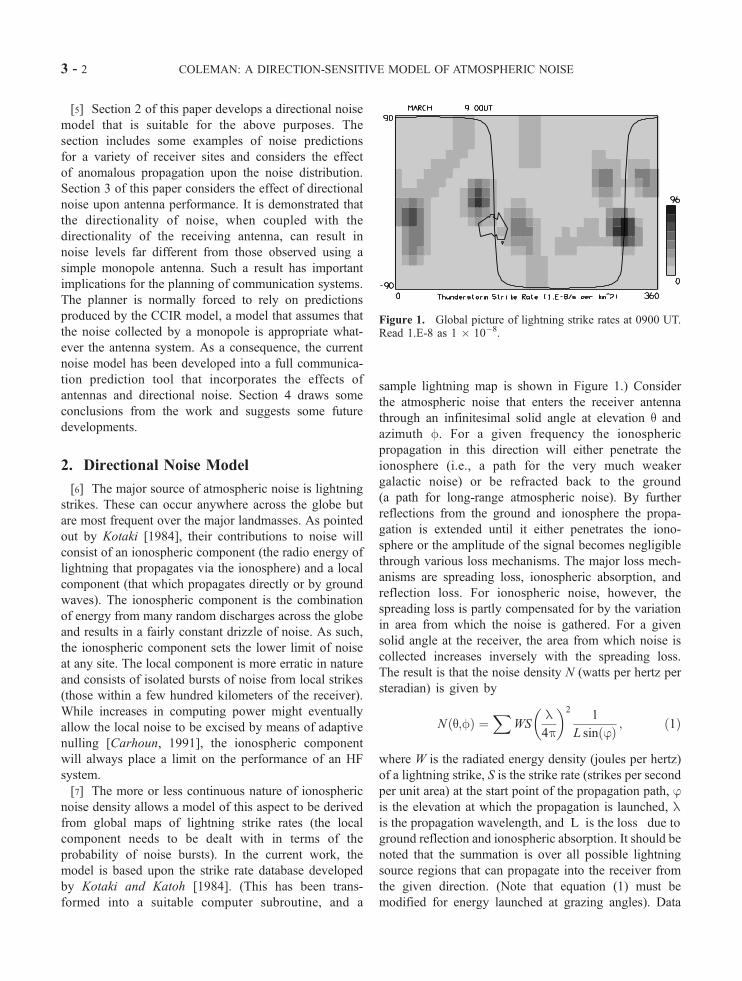
sample lightning map is shown in Figure 1.) Consider

the atmospheric noise that enters the receiver antenna

through an infinitesimal solid angle at elevation q and

azimuth f. For a given frequency the ionospheric

propagation in this direction will either penetrate the

ionosphere (i.e., a path for the very much weaker

galactic noise) or be refracted back to the ground

(a path for long-range atmospheric noise). By further

reflections from the ground and ionosphere the propa-

gation is extended until it either penetrates the iono-

sphere or the amplitude of the signal becomes negligible

through various loss mechanisms. The major loss mech-

anisms are spreading loss, ionospheric absorption, and

reflection loss. For ionospheric noise, however, the

spreading loss is partly compensated for by the variation

in area from which the noise is gathered. For a given

solid angle at the recei ver, the area from which noise is

collected increases inversely with the spreading loss.

The result is that the noise density N (watts per hertz per

steradian) is given by

N q;fð Þ ¼X

WSl4p

� �21

L sin jð Þ ; ð1Þ

where W is the radiated energy density (joules per hertz)

of a lightning strike, S is the strike rate (strikes per second

per unit area) at the start point of the propagation path, jis the elevation at which the propaga tion is launched , lis the propagation wavelength, and L is the loss due toground reflection and ionospheric absorption. It should be

noted that the summation is over all possible lightning

source regions that can propagate into the receiver from

the given direction. (Note that equation (1) must be

modified for energy launched at grazing angles). Data

Figure 1. Global picture of lightning strike rates at 0900 UT.Read 1.E-8 as 1 � 10�8.

3 - 2 COLEMAN: A DIRECTION-SENSITIVE MODEL OF ATMOSPHERIC NOISE

given by Jursa [1985] suggest a value of 2 � 10�6 J/Hz

for W at 10 MHz and 10�5 J/Hz at 2.5 MHz.[8] An important aspect of the noise model is the

ionospheric propagation tool that is used to estimate

the origin of energy arriving from a particular direction.

This tool is described by Coleman [1998] and employs a

two-dimensional (2-D) ray tracing tool together with an

ionospheric model [Coleman, 1997] in which the elec-

tron density is described by Chapman layers and layer

parameters are derived from the parameter maps of the

international reference ionsophere 1990 model [Bilitza,

1990]. Propagation calculations also provide the infor-

mation that is required to estimate the various losses. The

ground reflection part of the loss L is given by

Lr ¼ 10 log10Rvj j2þ Rhj j2

2

!; ð2Þ

where

Rv ¼n2 sinj� n2 � cos2 jð Þ1=2

n2 sinjþ n2 � cos2 jð Þ1=2;

Rh ¼sinj� n2 � cos2 jð Þ1=2

sinjþ n2 � cos2 jð Þ1=2;

with n2 = er � j18,000s/f, where er is the relative

dielectric constant of the Earth surface (80 for sea and an

assumed value of 15 for land), s is the conductivity of

the surface (5 S/m for sea and an assumed value of

0.01 S/m for land), and f is the propagation frequency. In

addition, the part of L due to ionospheric absorption is

calculated from the expression [Lucas and Haydon,

1966]

La ¼677:2 exp �2:937þ 0:8445f0Eð Þ � 0:04½

f þ fLð Þ1:98þ10:2h i

cosf100

; ð3Þ

where fL is the gyrofrequency, f0E is the E region critical

frequency, and f100 is the angle between the propagation

path and the vertical at an altitude of 100 km. The above

expression accounts for the absorption in the D and E

regions, but there will also be considerable deviative

absorption in the F region for some propagation. In the

present work, this additional absorption is estimated

according to 0.01(P0 � P) [Davies, 1990], where P0 and

P are the group and phase paths, respectively. (Note that

Lr and La are given in terms of decibels.)

[9] Figure 2 shows the distribution of lightning strikes

during dusk (0900 UT) for ranges up to 14,000 km out

from Alice Springs (central Australia). The circles on the

map denote range intervals of 2000 km, and strong

lightning sources in the equatorial regions of America,

Africa, and Southeast Asia will be noted. Figure 3 shows

the resulting noise distribution over the skyward hemi-

sphere for a frequency of 11 MHz, as calculated by the

above model. The Southeast Asian sources result in

strong noise from northwesterly directions, but it is clear

that ionospheric propagation limits the noise to the lower

elevations. Fairly strong noise is also evident from the

east and southeast, and this is a result of good nighttime

propagation across the Pacific Ocean. This propagation

causes the low-level sources in this region to have an

Figure 2. Lightning strike rates at dusk, centered on AliceSprings. SSN, sunspot number.

Figure 3. Directional noise distribution, as seen from AliceSprings at dusk.

COLEMAN: A DIRECTION-SENSITIVE MODEL OF ATMOSPHERIC NOISE 3 - 3

appreciable cumulative effect. Since radio waves from

sources in the direction of Africa must travel through a

significant amount of daylight, this noise is heavily

reduced by absorption. Consequently, there is very little

noise from the southwest sector. The effect of the losses

can be better seen in Figure 4, which shows the propaga-

tion gain (the combined effect of propagation losses such

as spreading, absorption, and reflection) for transmissions

from points out to 14,000 km. The above simulations are

supported by limited directional noise observations per-

formed using the frequency management system of the

Jindalee over the horizon radar at Alice Springs (P. S.

Whitham, Defense Science and Technology Organisation

Australia, private communication, 2000). These observa-

tions also show the strongest noise coming from the

northwest and southeast sectors with total variations of

more than 10 dB in azimuth. Figure 5 shows the simulated

noise distribution for a time later in the evening (1200UT),

from which it will be noted that there is increased noise

from Southeast Asia (to the northwest) due to the

increased nighttime propagation in this direction.

[10] Figure 6 shows some typical propagation paths to

the lightning sources in Southeast Asia (all of them

exclusively in nighttime and so little affected by absorp-

tion). The dashed curve indicates the lightning strike rate,

from which it is clear that there are good propagation

paths to the most active regions. This is not always the

case, as is illustrated by Figure 7. This figure shows

propagation from Darwin, in the north of Australia,

toward Southeast Asia. It will be noted that the effect of

the equatorial anomaly (the peaks of electron density to

the north and south of the geomagnetic equator) is to

cause a considerable portion of the propagation to skip

over the major thunderstorm sources. This will result in

noise holes at low elevations, as can be seen from the

directional noise distribution of Figure 8. The requisite

chordal propagation is a well-established, and frequent,

phenomenon in equatorial regions [Davies, 1990], and so

the possibility of such holes is strong. If they exist, they

could offer the possibility of low-power long-range com-

munication for a system with suitably limited elevation

response.

[11] An additional example of a noise distribution is

shown in Figure 9. The figure shows the simulated noise

for a receiver location slightly to the northwest of Boston

(United States) during a winter morning. This simulation

was chosen to coincide with the data collected by Keller

Figure 4. Propagation gain for signals reaching Alice Springsat dusk.

Figure 5. Directional noise distribution, as seen from AliceSprings in midevening.

Figure 6. Propagation paths from Alice Springs to lightningsources.


[1991] on an L-shaped directional receiving array. This

array geometry allowed Keller to infer the distribution of

noise over the skyward hemisphere. It will be noted that

the simulations show strong noise sources to the south

and to the northwest, but much reduced noise in the

northeast. This result is consistent with the observations

of Keller and strongly suggests that much of the observed

noise was atmospheric in origin. The simulated results

also show the atmospheric noise to be confined to

elevations below about 45�, strongly supporting Keller’s

inference that the higher noise levels were caused by

energy arriving through ionospheric reflections. Figure 10

shows the lightning sources that contribute to the

observed noise. It will be noted that there is a strong

density of strikes immediately to the south. The effect of

these sources will, however, be moderated by strong

daytime ionospheric absorption. Other sources farther to

the south and west will require several ionospheric hops to

Figure 7. Propagation paths from Darwin to lightning sources.

Figure 8. Directional noise distribution, as seen from Darwinin midevening.

Figure 9. Directional noise distribution, as seen from Bostonin the morning.


reach the receiver and so will be even more heavily

attenuated. Consequently, even though there are

extremely strong thunderstorm regions in South America,

these will have very little impact upon the noise spectrum

at this time of day. While the sources in the northeast

quadrant have a much lower strike rate than those imme-

diately to the south, the closer proximity to the day/night

transition will mean much lower signal attenuation and

hence a significant contribution to the noise environment.

The simulations of Figure 9 refer to a time that is well after

dawn, and the daytime attenuation has much reduced the

possible effects of ionospherically propagated noise. As a

consequence, the azimuthal variation of noise is little

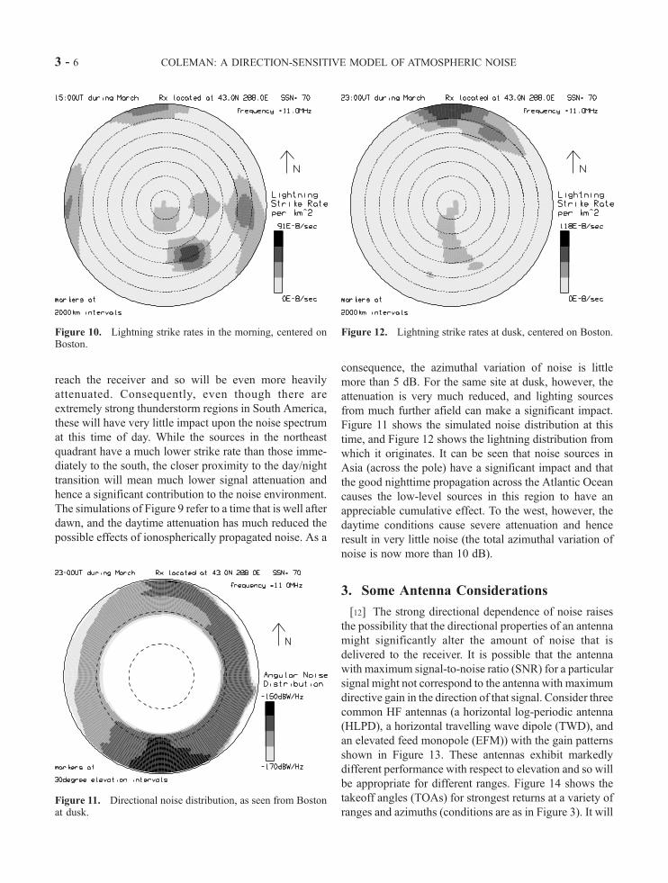
more than 5 dB. For the same site at dusk, however, the

attenuation is very much reduced, and lighting sources

from much further afield can make a significant impact.

Figure 11 shows the simulated noise distribution at this

time, and Figure 12 shows the lightning distribution from

which it originates. It can be seen that noise sources in

Asia (across the pole) have a significant impact and that

the good nighttime propagation across the Atlantic Ocean

causes the low-level sources in this region to have an

appreciable cumulative effect. To the west, however, the

daytime conditions cause severe attenuation and hence

result in very little noise (the total azimuthal variation of

noise is now more than 10 dB).

3. Some Antenna Considerations

[12] The strong directional dependence of noise raises

the possibility that the directional properties of an antenna

might significantly alter the amount of noise that is

delivered to the receiver. It is possible that the antenna

with maximum signal-to-noise ratio (SNR) for a particular

signal might not correspond to the antenna with maximum

directive gain in the direction of that signal. Consider three

common HF antennas (a horizontal log-periodic antenna

(HLPD), a horizontal travelling wave dipole (TWD), and

an elevated feed monopole (EFM)) with the gain patterns

shown in Figure 13. These antennas exhibit markedly

different performance with respect to elevation and so will

be appropriate for different ranges. Figure 14 shows the

takeoff angles (TOAs) for strongest returns at a variety of

ranges and azimuths (conditions are as in Figure 3). It will

Figure 10. Lightning strike rates in the morning, centered onBoston.

Figure 11. Directional noise distribution, as seen from Bostonat dusk.

Figure 12. Lightning strike rates at dusk, centered on Boston.


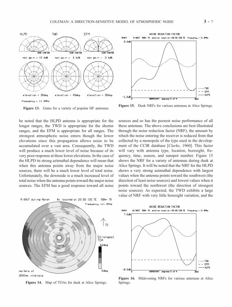
be noted that the HLPD antenna is appropriate for the

longer ranges, the TWD is appropriate for the shorter

ranges, and the EFM is appropriate for all ranges. The

strongest atmospheric noise enters though the lower

elevations since this propagation allows noise to be

accumulated over a vast area. Consequently, the TWD

will produce a much lower level of noise because of its

very poor response at these lower elevations. In the case of

the HLPD its strong azimuthal dependence will mean that

when this antenna points away from the major noise

sources, there will be a much lower level of total noise.

Unfortunately, the downside is a much increased level of

total noise when the antenna points toward the major noise

sources. The EFM has a good response toward all noise

sources and so has the poorest noise performance of all

these antennas. The above conclusions are best illustrated

through the noise reduction factor (NRF), the amount by

which the noise entering the receiver is reduced from that

collected by a monopole of the type used in the develop-

ment of the CCIR database [Clarke, 1960]. This factor

will vary with antenna type, location, boresight, fre-

quency, time, season, and sunspot number. Figure 15

shows the NRF for a variety of antennas during dusk at

Alice Springs. It will be noted that the NRF for the HLPD

shows a very strong azimuthal dependence with largest

values when the antenna points toward the southwest (the

direction of least noise sources) and lowest values when it

points toward the northwest (the direction of strongest

noise sources). As expected, the TWD exhibits a large

value of NRF with very little boresight variation, and the

Figure 13. Gains for a variety of popular HF antennas.

Figure 14. Map of TOAs for dusk at Alice Springs.

Figure 15. Dusk NRFs for various antennas at Alice Springs.

Figure 16. Midevening NRFs for various antennas at AliceSprings.


EFM has a noise performance that is very little different

from the CCIR monopole. Figure 16 shows the same site

during midevening, from which it will be noted that the

noise from Southeast Asia is now dominant. The worst

performance for the HLPD is still toward the northwest,

but there is a considerable improvement in virtually all

other directions. In addition, there is a small improvement

in the performance of the TWD. A further example is

given in Figure 17, which shows the early evening NRF

performance for antennas located at Darwin. It will be

noted that there is considerable change in antenna per-

formance from that exhibited at Alice Springs. This is a

direct result of the greatly changed propagation conditions

due to the proximity of the equatorial anomaly. In partic-

ular, it will be noted that there is a decreased performance

in the TWD due to the greater amount of noise that enters

through the higher elevation angles.

[13] A further issue arises when considering the recep-

tion of HF signals via an array-based antenna. Normal

beam-forming weights are calculated by optimizing the

SNR under the assumption that the noise is isotropic

(directionally white). For HF this is clearly not the best

approach, and the optimization should be based on

direction-varying (colored) noise (see Cox et al. [1987]

for examples of such beam-forming techniques). The

impact of such an optimization can be seen in

Figure 18, which shows the effective directivity (direc-

Figure 17. Midevening NRF for various antennas at Darwin.

Figure 18. Comparison of effective gains for arrays based onwhite and colored noise.

Figure 19. Directivity of a beam optimized on white noise.

Figure 20. Directivity of a beam optimized on mideveningcolored noise.


tivity plus noise reduction factor) for an 6 � 6 array of

monopole elements steered to an elevation of 15� and

swept around through 360�. (The array elements were

separated by 0.4 of a wavelength and, propagation

conditions were the same as for Figure 5.) Also included

is the effective gain that results when the beam forming is

achieved by constant phase increments between elements

in both array dimensions. It will be noted that there can

be considerable improvement in effective gain (2 to 5

dB) when the directional noise distribution is used for

optimization. Figures 19 and 20 show the directivity

patterns of the arrays when the beam is steered toward

the northeast. It will be noted from Figure 20 that the

array based on colored noise achieves its increase in SNR

by placing the sidelobes in directions where there is least

noise (the higher elevations in particular).

[14] An important aspect of the validation of the

current directional model has been the comparison of

its predictions of total noise with those of the CCIR

model (nonatmospheric contributions are taken from the

CCIR model). Kotaki [1984] considered some represen-

tative examples for which noise observations were avail-

able. Table 1 shows some comparisons of effective

antenna noise factor Fa for midevening at sites in Japan

(36.5�N, 140.5�E), the United States (40.1�N, 105.1�Wand 22.0�N, 159.7�W), Australia (30.6�S, 130.4�E),Sweden (59.5�, 17.3�E), and Singapore (1.3�S,103.8�E). The midevening time is when the effects of

atmospheric noise are at their strongest and so a good test

of the models. Included in Table 1 are noise factor results

derived from the CCIR model, the Kotaki model, the

current model, and some observations. The effective

antenna noise factor is defined by

Fa ¼ 10 log10Pn

kT0

� �;

where Pn is the noise collected by a lossless antenna in a

1 Hz bandwidth, k is the Boltzmann’s constant, and T0 is

a reference temperature of 288 K.

[15] It will be noted that the predictions of the current

model compare favorably with those of other models and

perform significantly better than the CCIR model in

several cases. Some comparisons with noise observations

on a frequency of 10 MHz for a site near Alice Springs in

central Australia (133.7�E, 23.5�S) are given in Table 2

(P. S. Whitham, private communication, 2000).

[16] It will be noted that the current model gives a fairly

accurate representation of all the above observed results

but that the CCIR model gives a significant overestimate

at the time of the dusk terminator. (It should be noted that

Kotaki [1984] also found situations where his model gave

significantly better predictions than CCIR estimates of

noise, as can be seen from Table 1.) In deriving the

estimates of noise for comparison with the CCIR model it

was necessary to add corrections due to the directive gain

of the antenna used in the CCIR observations (a broad-

band monopole over a radial ground system). The low-

elevation directive gains of this antenna were found to be

quite sensitive to the nature of the ground under the

antenna. Plausible variations in ground conductivity were

found to cause several decibels of deviation in noise

estimates for circumstances where there existed a large

amount of low-elevation noise. As a consequence, it is

likely that some of the seasonal variation in CCIR noise

could be a result of variations in site conditions. In the

current work, however, a representative value of 0.01 S/

m was assumed for ground conductivity, and 15 was

assumed for relative permittivity.

4. Conclusion

[17] The current paper has developed a model for the

atmospheric component of noise at HF frequencies. Not

only has this model given predictions that are in agree-

ment with the standard CCIR model in most of the test

cases, but it has also improved upon some of the

anomalous predictions. More importantly, however, the

model is able to address the issue of the directionality of

noise. This issue has been shown to be extremely

Table 1. Comparison Between Observation and Noise Model

Prediction for Various Locations Around the Worlda

Location Frequency,MHz

CCIRFa

Kotaki [1984]Fa

CurrentFa

ObservedFa

35�N, 141�E 2.5 57 60 53 5635�N, 141�E 5.0 50 51 53 5435�N, 141�E 10.0 40 40 42 441�S, 104�E 2.5 68 66 63 6131�S, 130�E 2.5 55 62 59 5960�N, 17�E 2.5 51 56 57 5222�N, 160�W 2.5 54 54 49 5040�N, 105�W 2.5 60 61 57 60

aFa values are given in decibels.

Table 2. Comparison Between Observation and Noise Model

Prediction for Alice Springsa

Local Time Current Fa CCIR Fa Observed Fa

1730 36 43 341900 45 46 452300 43 43 42

aFa values are given in decibels.


important when considering the performance of antennas

in receive applications. In particular, the directionality of

noise, when coupled with the directionality of the

antenna gain, can result in the system collecting an

amount of noise that is greatly different from the iso-

tropic case (the basis of CCIR estimates). In many cases

the amount by which CCIR noise must be adjusted has

been found to be quite large, and this serves to emphasize

the need for consideration of noise directionality in HF

system performance prediction.

[18] The directional noise model has been developed

into a performance prediction model for HF systems. The

model uses antenna gain patterns together with the

directional distribution of noise in order to estimate the

noise that enters the receiver. This is combined with

propagation predictions and other system parameters in

order to estimate the SNR that will be available at the

receiver. At present, the noise estimates are based on

median maps of thunderstorm activity and ionospheric

parameters. As a consequence, the current model will

only provide a median picture of noise that can, at best,

provide the planner with a ‘‘typical’’ system behavior. In

the future, however, it may be possible to use meteoro-

logical forecasts to provide more effective short-term

predictions of thunderstorms [Warber and Prasad,

1997] and hence of noise. If these predictions are coupled

with short-term forecasts of ionospheric behavior (based

on ionosonde observations), it should be possible to

derive effective short-term predictions of HF system

performance.

[19] Acknowledgments. The author would like to thankreferees for helpful comments.

References

Bilitza, D., International reference ionosphere 1990, Rep. 90–

22, Natl. Space Sci. Data Cent., Greenbelt, Md., 1990.

Carhoun, D. O., Adaptive nulling and spatial spectral estima-

tion using an iterated principle components decomposition,

paper presented at IEEE International Conference on Acous-

tics, Speech and Signal Processing, IEEE Signal Process.

Soc., Toronto, Canada, 1991.

Clarke, C., Atmospheric noise structure, Electron. Technol., 37,

197–204, 1960.

Coleman, C. J., On the simulation of backscatter ionograms, J.

Atmos. Sol. Terr. Phys., 59, 2089–2099, 1997.

Coleman, C. J., A ray tracing formulation and its application to

some problems in over-the-horizon radar, Radio Sci., 33,

1187–1197, 1998.

Coleman, C. J., The directionality of atmospheric noise and its

impact upon an HF receiving system, in Proceedings of the

8th International Conference on HF Radio Systems and

Techniques, IEE Conf. Publ., 474, 363–366, 2000.

Cox, H., R. M. Zeskind, and M. M. Owen, Robust adaptive

beamforming, IEEE Trans. Acoust. Speech Signal Process.,

ASSP-35, 1365–1375, 1987.

Davies, K., Ionospheric Radio, IEE Electromagn. Waves Ser.,

vol. 31, Peter Peregrinus, London, 1990.

International Radio Consultative Committee (CCIR), World

distribution and characteristics of atmospheric radio noise

data, Rep. 322, Int. Radio Consult. Comm., Int. Telecom-

mun. Union, Geneva, 1964.

International Telecommunication Union (ITU), Radio noise,

ITU-R Rep. P.372, Geneva, 1999.

Jursa, A. S. (Ed.), Handbook of Geophysics and the Space

Environment, Air Force Geophys. Lab., Air Force Syst.

Command, U.S. Air Force, Bedford, Mass., 1985.

Keller, C. M., HF noise environment models, Radio Sci., 26,

981–995, 1991.

Kotaki, M., Global distribution of atmospheric radio noise

derived from thunderstorm activity, J. Atmos. Terr. Phys.,

46, 867–877, 1984.

Kotaki, M., and C. Katoh, The global distribution of thunder-

storm activity observed by the Ionosphere Satellite (ISS-b),

J. Atmos. Terr. Phys., 45, 833–850, 1984.

Lucas, D. L., and G. W. Haydon, Predicting statistical perfor-

mance indexes for high frequency telecomunications sys-

tems, ESSA Tech. Rep. IER 1-ITSA, Natl. Oceanic and

Atmos. Admin., Silver Spring, Md., 1966.

Warber, C. R., and B. Prasad, Forecasting global lightning for

atmospheric noise prediction, Radio Sci., 32, 2027–2036,

1997.

��C. J. Coleman, Electrical and Electronic Engineering

Department, University of Adelaide, South Australia 5005,

Australia. ([email protected])


A direction-sensitive model of atmospheric noise and its ...

Documents

Transcript of A direction-sensitive model of atmospheric noise and its ...