A Covariance Estimator for Small Sample Size Classification Problems

and Its Application to Feature Extraction

Bor-Chen Kuo

School of Electrical and Computer Engineering

Purdue University, West Lafayette, Indiana 47907-1285

Tel: 765-494-9217

Email: borchen@ecn.purdue.edu

David A. Landgrebe,

School of Electrical and Computer Engineering

Purdue University, West Lafayette, Indiana 47907-1285

Tel: 765-494-3486

Email: landgreb@ecn.purdue.edu

Copyright © 2002 IEEE. Reprinted from IEEE Transactions on Geoscience andRemote Sensing. Vol. 40, No. 4, pp 814-819, April 2002. This material is postedhere with permission of the IEEE. Such permission of the IEEE does not in anyway imply IEEE endorsement of any of Purdue University's products or services.Internal or personal use of this material is permitted. However, permission toreprint/republish this material for advertising or promotional purposes or forcreating new collective works for resale or redistribution must be obtained fromthe IEEE by sending a blank email message to pubs-permissions@ieee.org.

By choosing to view this document, you agree to all provisions of the copyrightlaws protecting it.

- 1 -

June 20, 2002

A Covariance Estimator for Small Sample Size Classification Problems

and Its Application to Feature Extraction1

Bor-Chen Kuo, Member, IEEE and David A. Landgrebe, Life Fellow, IEEE

Abstract

A key to successful classification of multivariate data is the defining of an accurate

quantitative model of each class. This is especially the case when the dimensionality of the data

is high, and the problem is exacerbated when the number of training samples is limited. For the

commonly used quadratic maximum likelihood classifier the class mean vectors and covariance

matrices are required and must be estimated from the available training samples. In high

dimensional cases it has been found that feature extraction methods are especially useful, so as to

transform the problem to a lower dimensional space without loss of information, however, here

too, class statistics estimation error is significant. Finding a suitable regularized covariance

estimator is a way to mitigate these estimation error effects. The main purpose of this work is to

find an improved regularized covariance estimator of each class with the advantages of LOOC,

and BLOOC. Besides, using the proposed covariance estimator to improve the linear feature

extraction methods when the multivariate data is singular or nearly so is demonstrated. This

work is specifically directed at analysis methods for hyperspectral remote sensing data.

1 The work described in this paper was sponsored in part by the National Imagery and Mapping Agency undergrant NMA 201-01-C-0023

- 2 -

June 20, 2002

1 Introduction

As new sensor technology has emerged over the past few years, high dimensional

multispectral data with hundreds of bands have become available. For example, the AVIRIS

system2 gathers image data in 210 spectral bands in the 0.4-2.4 µm range. Compared to the

previous data of lower dimensionality (less than 20 bands), this hyperspectral data potentially

provides a wealth of information. However, it also raises the need for more specific attention to

the data analysis procedure if this potential is to be fully realized.

Among the ways to approach hyperspectral data analysis, a useful processing model that

has evolved in the last several years [1] is shown schematically in Figure 1. Given the

availability of data (box 1), the process begins by the analyst specifying what classes are desired,

usually by labeling training samples for each class (box 2). New elements that have proven

important in the case of high dimensional data are those indicated by boxes in the diagram

marked 3 and 4. These are the focus of this work and will be discussed in more detail shortly,

however the reason for their importance in this context is as follows. Classification techniques in

pattern recognition typically assume that there are enough training samples available to obtain

reasonably accurate class descriptions in quantitative form. Unfortunately, the number of training

samples required to train a classifier for high dimensional data is much greater than that required

for conventional data, and gathering these training samples can be difficult and expensive.

Therefore, the assumption that enough training samples are available to accurately estimate the

2 Airborne Visible and Infrared Imaging Spectrometer system, built and operated by the NASA Jet PropulsionCenter.

- 3 -

June 20, 2002

class quantitative description is frequently not satisfied for high dimensional data. There are

many types of classification algorithms used on such data. Perhaps the most common is the

quadratic maximum likelihood algorithm. For such a quadratic classifier, user classes must be

modeled by a set of subclasses, and the mean vector and covariance matrix of each subclass are

the parameters that must be estimated from training samples. Usually the ML estimator is used.

When the dimensionality of data exceeds the number of training samples, the ML covariance

estimate is singular and cannot be used, however even in cases where the number of training

samples is only two or three times the number of dimensions, estimation error can be a

significant problem.

Figure 1. A schematic diagram for a hyperspectral data analysis procedure.

There are several ways to overcome this difficulty. In [2], these techniques are categorized

into three groups:

5 FeatureSelection

1 MultispectralData

6 Classifier4 Class ConditionalFeature Extraction

2 Label TrainingSamples

3 Determine QuantitativeClass Descriptions

- 4 -

June 20, 2002

a. Dimensionality reduction by feature extraction or feature selection.

b. Regularization of sample covariance matrix (e.g. [3], [4], [5], [6], [7]).

c. Structurization of a true covariance matrix described by a small number of parameters

[2].

The purposes of this study are to find an improved regularized covariance estimator of each class

that is invertible and with the advantages of LOOC [5], [6] and BLOOC [7] (box 3 of the figure),

and show that linear feature extraction procedures (box 4) can be improved by using the

proposed regularized covariance estimator.

2 Previous methods for regularization

Several methods for regularization have appeared in the literature. Regularized

Discriminant Analysis (RDA) [3] is a two-dimensional optimization over four-way mixtures of

the sample covariance, common covariance, the identity matrix times the average diagonal

element of the common covariance, and the identity matrix times the average diagonal element

of the sample covariance. The pair of mixing parameters is selected by cross-validating on the

total number of misclassifications based on available training samples. Even though this

procedure has the benefit of directly relating to the classification accuracy, it is computationally

expensive, and the same mixing parameters must be used for all classes.

Leave-One-Out Covariance Estimator (LOOC; [5],[6] ) uses the following mixture scheme.

- 5 -

June 20, 2002

ˆ S i(ai ) =

(1 -a i)diag(Si ) + aiSi 0 £ ai £1(2 -a i)Si + (ai -1)S 1£ a i £ 2(3 - ai)S + (ai - 2)diag(S) 2 £ ai £ 3

Ï

Ì Ô Ô

Ó Ô Ô

(1)

The mean of class i, without sample k, is Â≠=-

=iN

kjj

jii

ki xN

m1

,/ 11 , where the notation /k

indicates the quantity is computed without sample k. The sample covariance of class i, without

sample k, is

( )( )Tkiji

N

kjj

kijii

ki mxmxN

i

/,1

/,/ 21

---

=S Â≠=

(2)

and the common covariance, without sample k from class i, is

ki

L

ijj

jki LLS /

1/

11S+

˜˜˜

¯

ˆ

ÁÁÁ

Ë

ÊS= Â

≠=

(3)

The proposed estimate for class i, without sample k, can then be computed as follows:

( )( ) ( )( ) ( )( ) ( )Ô

Ó

ÔÌ

Ï

£<-+-

£<-+S-

££S+S-

=

32 )(23

21 12

10 1

//

//

//

/

ikiikii

ikiikii

ikiikii

iki

SdiagS

S

diag

C

aaa

aaa

aaa

a (4)

The mixing parameter ai is determined by maximizing the average leave-one-out log likelihood

of each class:

)]( ,|(ln[1

//1

ikiki

N

kk

ii Cmxf

NLOOL

i

aÂ=

= (5)

- 6 -

June 20, 2002

As aforementioned, in the process of selecting the mixing parameter values by maximizing the

leave-one-out average log likelihood, the class covariance estimates can be determined

independently, and then each class can have a mixing parameter that is optimal in terms of

available training samples. Overall, classes with more training samples only need a small amount

of bias, while classes with very few training samples need more bias.

BLOOC [7] is a modification of LOOC. LOOC was found to work well for well-trained

classifiers, however, it is sensitive to outliers. In practice outliers frequently occur in cases where

the class list is not exhaustive, such that the missing classes constitute outliers to the defined

classes. Thus the following scheme was devised.

ÔÔÔ

Ó

ÔÔÔ

Ì

Ï

£<-+-

<£-+-

££+-

=S

32 )(

)2()3(

21 (t))1()2(

10 )(

)1(

)(ˆ *

iii

ipiii

iiii

i

ii

Ip

StrS

SS

SIp

Str

aaa

aaa

aaa

a

where t can be expressed as the function of ai , t =(ai -1) fi - ai( p +1)

2 - ai, where p is the

dimensionality and fi = Ni -1, which represents the degree of freedom in Wishart distributions,

and the pooled covariance matrices are determined under a Bayesian context and can be

represented as:

Sp*(t) =

fi

fi + t - p -1i =1

L

ÂÈ

Î Í Í

˘

˚ ˙ ˙

-1fiSi

fi + t - p -1i=1

L

 (6)

- 7 -

June 20, 2002

The first difference between LOOC and BLOOC is that LOOC uses the diagonal entries of

covariance matrices but BLOOC, like RDA, uses the trace of covariance matrices. Second, in

LOOC, the maximum likelihood common covariance estimator is used, but, in BLOOC, the

maximum a posterior common covariance estimator (Sp* ) is added. From [4], Sp

* tends to

mitigate the outlier problem, and so does BLOOC. The criterion function of BLOOC is the same

as that of LOOC.

A comparison of the performances of RDA, LOOC, and BLOOC is given in [8]. This

comparison shows that LOOC performance is better than RDA in most situations, and BLOOC

performs even better in special situations. In addition, computation time is decreasing in the

order RDA, BLOOC, and LOOC. According to both accuracy and computation, LOOC is a

better choice than the others. However, BLOOC has an advantage of being more resistant to

outliers in the training set.

3 Mixed Leave-One-Out Covariance (Mixed-LOOC) Estimators

3.1 Mixed-LOOC1

LOOC and BLOOC are the linear combination of two of the three matrices, and in some

situations, the difference between LOOC and BLOOC is in those matrices used to formulate the

regularized covariance estimator. Only using some of the six matrices will not perform well in all

situations. The basic idea of Mixed-LOOC is to use all six matrices to gain the advantages of

both LOOC and BLOOC. Hence the first proposed regularized covariance estimator, Mixed-

LOOC1, is

- 8 -

June 20, 2002

(pooled)matrix covariancecommon :

i class ofmatrix covariance :

dimensions ofnumber :

classes ofnumber :

,...,21 and 1 where

)()(

)()(

),,,,,(ˆ

S

S

p

L

L,ifedcba

SfSdiageIp

StrdScSdiagbI

p

Strafedcba

i

iiiiii

iiiiiiii

iiiiiiii

==+++++

+++++=S

(7)

The mixture parameters are determined by maximizing the average leave-one-out log

likelihood of each class:

))](ˆ ,|(ln[1

//1

ikiki

N

kk

ii mxf

NLOOL

i

qS= Â=

, where ),,,,,( iiiiiii fedcba=q (8)

3.2 Mixed-LOOC2

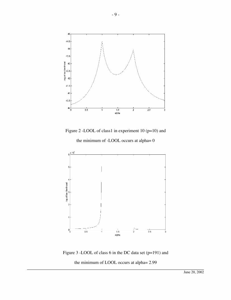
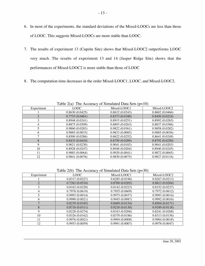
Since using Mixed-LOOC1 is computationally intensive, finding a more simplified

estimator will be more practical. It is shown in [8] that given two known matrices, the ML (not

Leave-One-Out) estimate of mixture parameters in LOOC and BLOOC are at the end points

( ia =0, 1, 2, or 3). Figures 2, and 3 illustrate the relationship between LOOL and the mixture

parameter, ai. The first figure is generated from a simulated data set; Figure 3 is based on a real

data set [8]. The detailed information about simulated and real data set is in the experiment

design section (section 4). In the case of Figure 2, the sample size is greater than the

dimensionality. For Figure 3, the sample size is less than the dimensionality. Figure 3 shows that

when the ML covariance estimator is singular, the optimal choice of LOOC parameter under

LOOL criteria is around the boundary points.

- 9 -

June 20, 2002

Figure 2 -LOOL of class1 in experiment 10 (p=10) and

the minimum of -LOOL occurs at alpha= 0

Figure 3 -LOOL of class 6 in the DC data set (p=191) and

the minimum of LOOL occurs at alpha= 2.99

- 10 -

June 20, 2002

Since a closed form solution for the parameter ai under the LOOL criteria is not available,

and based on the above observations, one of the six support matrices is chosen to be the

covariance estimator to reduce the computation time. The Mixed-LOOC2 is proposed as the

following form:

B)1(A)(ˆi iii aaa -+=S (9)

where SSdiagIp

StrSSdiagI

p

Strii

i or ),( ,)(

, ,)( ,)(

A = , )(or , B SdiagSi= and ia is close to

1. )(or , B SdiagSi= is chosen because if a class sample size is large, iS will be a better choice.

If total training sample size is less than the dimensionality, then the common (pooled) covariance

S is singular but has much less estimation error than iS . For reducing estimation error and

avoiding singularity, )(Sdiag will be a good choice. The selection criteria is the log leave-one-

out likelihood function:

))](ˆ ,|(ln[1

//1

ikiki

N

kk

ii mxf

NLOOL

i

aS= Â=

(10)

The algorithm to decide the Mixed-LOOC2 of each class is to compute LOOL of the 12

covariance estimator combinations, then choose the maximal one. This method needs less

computation time than the LOOC proposed in [5].

4 Experiment Design for Comparing LOOC, Mixed-LOOC1, and Mixed-LOOC2

In the following experiments, the grid method is used to estimate the mixture parameters of

LOOC and Mixed-LOOC1. The range of the parameter a in LOOC is from 0 to 3 and the grids

- 11 -

June 20, 2002

are a = [0, 0.25, 0.5, …, 2.75, 3]. There are six parameters in Mixed-LOOC1 and the ranges of

them are from 0 to 1. The grids of Mixed-LOOC1 are [0, 0.25, 0.5, 0.75, 1]. For Mixed-LOOC2,

the parameter a is set to 0.05. In the simulation experiments, performances of all three

covariance estimators are compared. Based on computational consideration, only the

performances of LOOC and Mixed-LOOC2 are compared for the real data experiments.

Experiments 1 to 12 are based on simulated data sets. Experiments 1 to 6 and experiments

7 to 12 are generated from the same normal distributions respectively. The mean vectors and

covariance matrices of experiments 1 to 6 (and 7 to 12) are the same as those six experiments in

[3]. See also Appendix B of [8]. The only difference between these two sets of experiments is

that experiment 1 to 6 are with equal training sample sizes in each class but experiments 7 to 12

are with different sample sizes in each class. Training and testing sample sizes of these

experiments are in Table 1. There are three different dimensionalities, p=10, 30, 60, in every

experiment. At each situation, 10 random training and testing data sets are generated for

computing the accuracies of algorithms, and the standard deviations of the accuracies.

Table 1 The Design of Sample SizeExperiments 1 ~ 6 Experiments 7 ~ 12

Sample Size Class 1 Class 2 Class 3 Class 1 Class 2 Class 3Training 10 10 10 30 10 5Testing 200 200 200 600 200 100

There are four different real data sets, the Cuprite site in western Nevada, an area of

geologic interest; Jasper Ridge in California, an ecological site; Indian Pine in NW Indiana, an

agricultural/forestry site; and the Washington, DC Mall, an urban site; in experiment 13 to 16

respectively. All real data sets have 191 bands. There are 8, 6, 6, and 7 classes used in the

- 12 -

June 20, 2002

Cuprite Site, Jasper Ridge Site, Indian Pine Site, and DC Mall, respectively. There are 20

training samples in each class. At each experiment, 10 training and testing data sets are selected

for computing the accuracies of algorithms, and the standard deviations of the accuracies.

5 Experiment Results

The simulated data results are displayed in Table 2(a), 2(b), 2(c). The real data results are

displayed in Table 2(d). They show the following.

1. In Table 2(a), (b), (c), the shadowed parts indicate that the differences of performances of

LOOC and Mixed-LOOC2 are larger than the standard deviation of Mixed-LOOC2. If the

difference is smaller than the standard deviation, we assume that the performances of these

methods have no significant difference.

2. All the experiments with significant differences (the shaded parts) indicate that Mixed-

LOOC outperformed LOOC.

3. The results of shaded parts show that the differences between Mixed-LOOC and LOOC

increase as the number of dimensions increases.

4. When the training sample sizes of the classes are unbalanced, Mixed-LOOC performed better

than LOOC in more situations.

5. Significant differences most often occurred in experiments 2, 7, and 8. Those are the

situations in which BLOOC has better performances than LOOC. Since the Mixed-LOOCs

are the union version of LOOC and BLOOC, based on these findings, we conclude that the

Mixed-LOOCs have advantages over LOOC and BLOOC and can avoid their disadvantages.

- 13 -

June 20, 2002

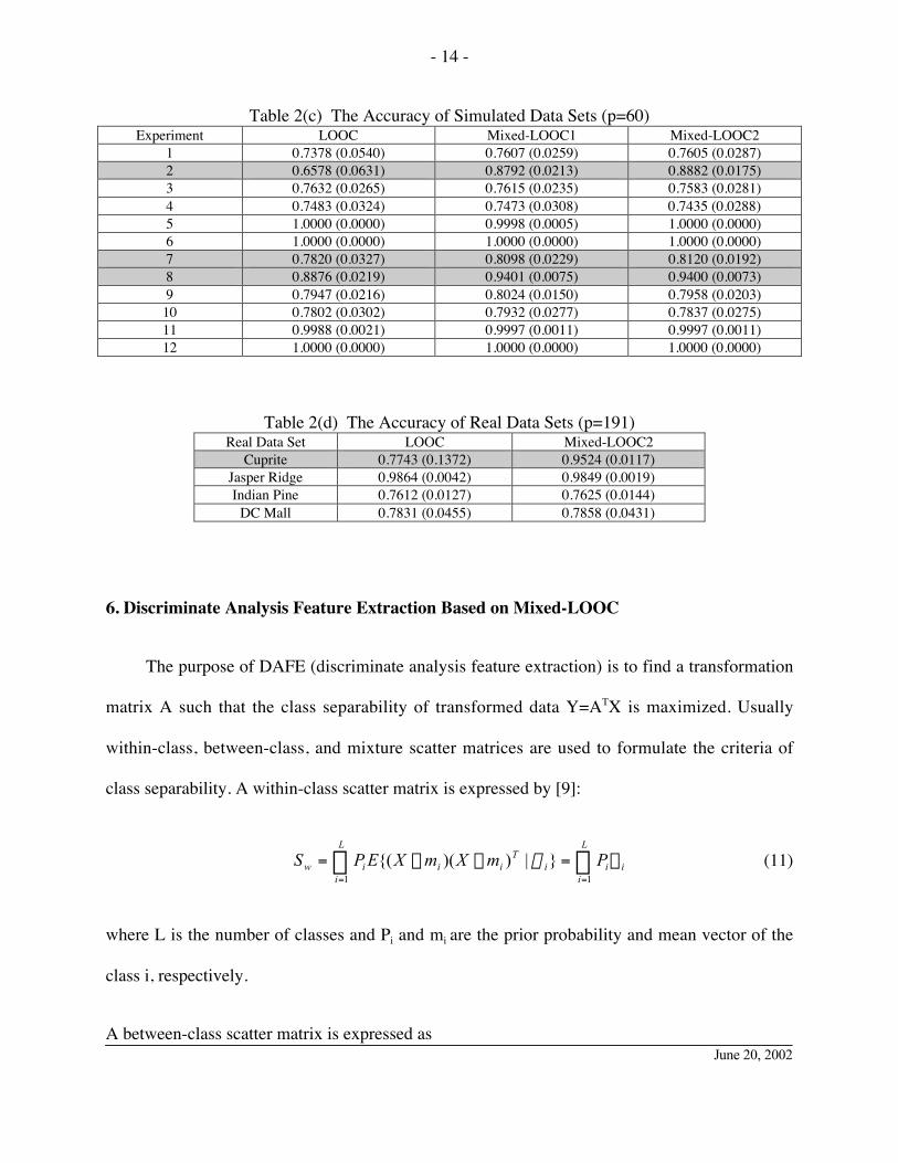
6. In most of the experiments, the standard deviations of the Mixed-LOOCs are less than those

of LOOC. This suggests Mixed-LOOCs are more stable than LOOC.

7. The results of experiment 13 (Cuprite Site) shows that Mixed-LOOC2 outperforms LOOC

very much. The results of experiment 13 and 14 (Jasper Ridge Site) shows that the

performances of Mixed-LOOC2 is more stable than those of LOOC

8. The computation time decreases in the order Mixed-LOOC1, LOOC, and Mixed-LOOC2.

Table 2(a) The Accuracy of Simulated Data Sets (p=10)Experiment LOOC Mixed-LOOC1 Mixed-LOOC2

1 0.8630 (0.0425) 0.8632 (0.0243) 0.8602 (0.0466)2 0.7753 (0.0481) 0.8373 (0.0180) 0.8450 (0.0224)3 0.8948 (0.0241) 0.8915 (0.0251) 0.8992 (0.0265)4 0.8875 (0.0309) 0.8893 (0.0263) 0.8837 (0.0386)5 0.9860 (0.0283) 0.9822 (0.0361) 0.9858 (0.0282)6 0.9885 (0.0033) 0.9833 (0.0085) 0.9885 (0.0036)7 0.8500 (0.0286) 0.8622 (0.0252) 0.8641 (0.0249)8 0.8433 (0.0410) 0.8750 (0.0289) 0.8792 (0.0250)9 0.9021 (0.0230) 0.9041 (0.0183) 0.9041 (0.0203)10 0.8928 (0.0247) 0.8948 (0.0204) 0.8940 (0.0245)11 0.9883 (0.0064) 0.9920 (0.0041) 0.9872 (0.0065)12 0.9841 (0.0076) 0.9830 (0.0075) 0.9827 (0.0116)

Table 2(b) The Accuracy of Simulated Data Sets (p=30)Experiment LOOC Mixed-LOOC1 Mixed-LOOC2

1 0.8317 (0.0227) 0.8285 (0.0196) 0.8267 (0.0213)2 0.7263 (0.0510) 0.8700 (0.0205) 0.8813 (0.0204)3 0.8162 (0.0220) 0.8142 (0.0223) 0.8152 (0.0237)4 0.7978 (0.0619) 0.7955 (0.0609) 0.7972 (0.0612)5 0.9993 (0.0014) 0.9975 (0.0037) 0.9993 (0.0014)6 0.9990 (0.0021) 0.9945 (0.0087) 0.9992 (0.0016)7 0.8239 (0.0345) 0.8469 (0.0154) 0.8504 (0.0171)8 0.8718 (0.0311) 0.9210 (0.0130) 0.9189 (0.0118)9 0.8228 (0.0274) 0.8343 (0.0206) 0.8241 (0.0268)10 0.8326 (0.0162) 0.8370 (0.0186) 0.8313 (0.0156)11 0.9976 (0.0021) 0.9994 (0.0008) 0.9984 (0.0018)12 0.9953 (0.0059) 0.9991 (0.0007) 0.9978 (0.0047)

- 14 -

June 20, 2002

Table 2(c) The Accuracy of Simulated Data Sets (p=60)Experiment LOOC Mixed-LOOC1 Mixed-LOOC2

1 0.7378 (0.0540) 0.7607 (0.0259) 0.7605 (0.0287)2 0.6578 (0.0631) 0.8792 (0.0213) 0.8882 (0.0175)3 0.7632 (0.0265) 0.7615 (0.0235) 0.7583 (0.0281)4 0.7483 (0.0324) 0.7473 (0.0308) 0.7435 (0.0288)5 1.0000 (0.0000) 0.9998 (0.0005) 1.0000 (0.0000)6 1.0000 (0.0000) 1.0000 (0.0000) 1.0000 (0.0000)7 0.7820 (0.0327) 0.8098 (0.0229) 0.8120 (0.0192)8 0.8876 (0.0219) 0.9401 (0.0075) 0.9400 (0.0073)9 0.7947 (0.0216) 0.8024 (0.0150) 0.7958 (0.0203)10 0.7802 (0.0302) 0.7932 (0.0277) 0.7837 (0.0275)11 0.9988 (0.0021) 0.9997 (0.0011) 0.9997 (0.0011)12 1.0000 (0.0000) 1.0000 (0.0000) 1.0000 (0.0000)

Table 2(d) The Accuracy of Real Data Sets (p=191)Real Data Set LOOC Mixed-LOOC2

Cuprite 0.7743 (0.1372) 0.9524 (0.0117)Jasper Ridge 0.9864 (0.0042) 0.9849 (0.0019)Indian Pine 0.7612 (0.0127) 0.7625 (0.0144)

DC Mall 0.7831 (0.0455) 0.7858 (0.0431)

6. Discriminate Analysis Feature Extraction Based on Mixed-LOOC

The purpose of DAFE (discriminate analysis feature extraction) is to find a transformation

matrix A such that the class separability of transformed data Y=ATX is maximized. Usually

within-class, between-class, and mixture scatter matrices are used to formulate the criteria of

class separability. A within-class scatter matrix is expressed by [9]:

i

L

iii

Tii

L

iiw PmXmXEPS S=--= ÂÂ

== 11

}|))({( w (11)

where L is the number of classes and Pi and mi are the prior probability and mean vector of the

class i, respectively.

A between-class scatter matrix is expressed as

- 15 -

June 20, 2002

Tii

L

iib mmmmPS ))(( 00

1

--= Â=

=Â Â-

= +=

--1

1 1

))((L

i

Tjiji

L

ijji mmmmPP (12)

where m0 represents the expected vector of the mixture distribution and is given by

i

L

ii mPXEm Â

=

==1

0 }{ (13)

Let XAY T= , then we have

ASAS wXT

wY = and ASAS bXT

bY = (14)

The optimal features are determined by optimizing the criterion given by

)( 11 bYwY SStrJ -= (15)

The optimum A must satisfy

)()( 11bYwYbXwX SSAASS -- = (16)

This is a generalized eigenvalue problem [10] and usually can be solved by the QZ algorithm.

But if the covariance is singular, the result will have a poor and unstable performance on

classification. In this section, the ML covariance estimate will be replaced by Mixed-LOOC

when it is singular. Then the problem will become a simple eigenvalue problem.

For convenience, denote DAFE based on ML estimators as DAFE, DAFE based on Mixed-

LOOC2 as DAFE-Mix2, Gaussian classifier based on ML estimators as GC, and Gaussian

classifier based on Mixed-LOOC2 estimators as GC-Mix2. Experiments 17 to 19 are for

determining the performances of DAFE-Mix2. The classification process in experiment 17 is to

- 16 -

June 20, 2002

use DAFE then GC, in experiment 18 use DAFE-Mix2 then GC, and in experiment 19 use

DAFE-Mix2 then GC-Mix2. The class sample sizes of experiment 18 and 19 are the same as

those of experiments 13 to 16 (Ni=20). Since using those sample sizes in DAFE will cause very

poor results, we increase the sample size of each class in Cuprite, Jasper Ridge, Indian Pine, and

DC Mall data sets up to 40. The number of features extracted from the original space is set to the

number of classes minus 1. The results of those experiments are shown in Table 3 and Figure 4.

Table 3 The Mean Accuracies and Standard Deviations of ExperimentsReal Data Set Exp17 DAFE+GC Exp18 DAFE-Mix2+GC Exp19 DAFE-Mix2+GC-Mix2

Cuprite 0.8943 (0.0205) 0.9474 (0.0194) 0.9627 (0.0196)Jasper Ridge 0.9127 (0.0243) 0.9782 (0.0120) 0.9876 (0.0036)Indian Pine 0.5727 (0.0156) 0.7547 (0.0316) 0.7562 (0.0191)

DC Mall 0.7392 (0.0530) 0.8691 (0.0282) 0.8600 (0.0345)

0.5

0.6

0.7

0.8

0.9

1

Cuprite JasperRidge

IndianPine

DCMall

Acc

urac

y

Exp17 DAFE+GC (Ni=40)

Exp18 DAFE-Mix2+GC(Ni=20)Exp19 DAFE-Mix2+GC-Mix2 (Ni=20)

Figure 4 The Mean Accuracies of Three Classification Procedures

From above results we find the following.

1. Using DAFE-Mix2 provides higher accuracy and, in most cases, smaller standard

deviation than using only DAFE.

- 17 -

June 20, 2002

2. Comparing Table 2(d) and Table 3, we find that in all data sets except the DC Mall sets,

using DAFE-Mix2 then GC or GC-Mix2 have similar results with only using GC-Mix2.

But the results for DC Mall show that using DAFE-Mix2 then GC or GC-Mix2 gave a

significant improvement.

3. From Table 3 and Figure 4, DAFE-Mix2 -GC-Mix2 looks like the best choice.

7 Concluding Comments

The singularity or near-singularity problem often occurs in the case of high dimensional

classification. From the above discussion, we know that finding a suitable regularized covariance

estimator is a way to mitigate this problem. Further, Mixed-LOOC2 has advantages over LOOC

and BLOOC and needs less computation than those two. The problems of class statistics

estimation error resulting from training sets of finite size grows rapidly with dimensionality, thus

making it desirable to use no larger feature space dimensionality than necessary for the problem

at hand, and therefore the importance of an effective, case-specific feature extraction procedure.

Usually DAFE cannot be used when the training sample size is less than dimensionality. The

new procedure, DAFE-Mix2, overcomes this shortcoming, and can provide higher accuracy

when the sample size is limited.

- 18 -

June 20, 2002

References

[1] David Landgrebe, "Information Extraction Principles and Methods for Multispectral and

Hyperspectral Image Data," Chapter 1 of Information Processing for Remote Sensing, edited

by C. H. Chen, published by the World Scientific Publishing Co., Inc., 1060 Main Street,River Edge, NJ 07661, USA 1999*.

[2] S. Raudys and A. Saudargiene, “Structures of the Covariance Matrices in Classifier Design”,

Advances in Pattern Recognition, A. Amin, D. Dori, P. Pudil, and H. Freeman, ed., BerlinHeidelberg: Springer-Verlag pp.583-592,1998.

[3] J.H. Friedman, “ Regularized Discriminant Analysis,” Journal of the American Statistical

Association, vol. 84, pp. 165-175, March 1989

[4] W. Rayens and T. Greene, “ Covariance pooling and stabilization for classification.”

Computational Statistics and Data Analysis, vol. 11, pp. 17-42, 1991

[5] J. P. Hoffbeck and D.A. Landgrebe, Classification of High Dimensional Multispectral Data,

Purdue University, West Lafayette, IN., TR-EE 95-14, May, 1995, pp.43-71*.

[6] J. P. Hoffbeck and D.A. Landgrebe, “ Covariance matrix estimation and classification with

limited training data” IEEE Transactions on Pattern Analysis & Machine Intelligence, vol

18, No. 7, pp. 763-767, July 1996*.

[7] S. Tadjudin and D.A. Landgrebe, Classification of High Dimensional Data with Limited

Training Samples, Purdue University, West Lafayette, IN., TR-EE 98-8, April, 1998, pp35-82*.

* Available for download in pdf format from http://dynamo.ecn.purdue.edu/~landgreb/publications.html.

- 19 -

June 20, 2002

[8] Bor-Chen Kuo and David Landgrebe, Improved Statistics Estimation And Feature Extraction

For Hyperspectral Data Classification, PhD Thesis and School of Electrical & ComputerEngineering Technical Report TR-ECE 01-6, December 2001 (88 pages)*,

[9] K. Fukunaga, Introduction to Statistical Pattern Recognition, San Diego: Academic PressInc., 1990.

[10] Moler, C. B. and G.W. Stewart, "An Algorithm for Generalized Matrix Eigenvalue

Problems", SIAM J. Numer. Anal., Vol. 10, No. 2, April 1973.

* Available for download in pdf format from http://dynamo.ecn.purdue.edu/~landgreb/publications.html.