A Conceptual Glacio-hydrological Model

HESSD2, 73–117, 2005

A conceptualglacio-hydrological

model

B. Schaefli et al.

Title Page

Abstract Introduction

Conclusions References

Tables Figures

J I

J I

Back Close

Full Screen / Esc

Print Version

Interactive Discussion

EGU

Hydrol. Earth Syst. Sci. Discuss., 2, 73–117, 2005www.copernicus.org/EGU/hess/hessd/2/73/SRef-ID: 1812-2116/hessd/2005-2-73European Geosciences Union

Hydrology andEarth System

SciencesDiscussions

A conceptual glacio-hydrological modelfor high mountainous catchmentsB. Schaefli, B. Hingray, M. Niggli, and A. Musy

Hydrology and Land Improvement Laboratory, Swiss Federal Institute of Technology,Lausanne, Switzerland

Received: 29 December 2004 – Accepted: 11 January 2005 – Published: 17 January 2005

Correspondence to: B. Schaefli ([email protected])

© 2005 Author(s). This work is licensed under a Creative Commons License.

73

http://www.copernicus.org/EGU/hess/hessd.htm

http://www.copernicus.org/EGU/hess/hessd/2/73/hessd-2-73_p.pdf

http://www.copernicus.org/EGU/hess/hessd/2/73/comments.php

http://www.copernicus.org/EGU/EGU.html

HESSD2, 73–117, 2005


model

B. Schaefli et al.

Title Page



Tables Figures

J I

J I

Back Close

Full Screen / Esc

Print Version


EGU

Abstract

In high mountainous catchments, the spatial precipitation and therefore the overall wa-ter balance is generally difficult to estimate. The present paper describes the structureand calibration of a semi-lumped conceptual glacio-hydrological model for the jointsimulation of daily discharge and annual glacier mass balance that represents a better5

integrator of the water balance. The model has been developed for climate change im-pact studies and has therefore a parsimonious structure; it requires three input timesseries – precipitation, temperature and potential evapotranspiration – and has 7 param-eters to calibrate. A multi-signal approach considering daily discharge and – if available– annual glacier mass balance has been developed for the calibration of these param-10

eters. The model has been calibrated for three different catchments in the Swiss Alpshaving glaciation rates between 37% and 52%. It simulates well the observed dailydischarge, the hydrological regime and some basic glaciological features, such as theannual mass balance.

1. Introduction15

Discharge estimation from highly glacierized catchments has always been a key hy-drological issue in the Swiss Alps, especially for the design and management of hy-dropower plants and for flood risk studies. However, the interest of scientists and civilengineers in this issue drastically decreased after the main period of dam constructionin the middle of the last century. Catchments subjected to a glacier regime show a20

very constant annual hydrological cycle, the start and the end of the melting seasonvarying little from year to year. For hydroelectricity production, the water managementtherefore rather relies on the long-term experience than on discharge simulations. Inthe nineties, land managers started asking for hydrological models able to simulaterunoff from these snow- and ice melt affected catchments for flood risk studies. In this25

context, the main interest was focused on rainfall and snowmelt induced processes and

74





HESSD2, 73–117, 2005


model

B. Schaefli et al.

Title Page



Tables Figures

J I

J I

Back Close

Full Screen / Esc

Print Version


EGU

on event-based discharge simulation (e.g. Consuegra et al., 1998). Recently, continu-ous runoff simulation from glacierized catchments has experienced a regain of interestamong scientists, hydropower and land managers, in particular in the context of climatechange impact studies (Willis and Bonvin, 1995; Singh and Kumar, 1997; Braun et al.,2000).5

In high mountainous catchments, discharge simulation is confronted with a majorchallenge: the available meteorological data is scarce – at high altitudes nearly inexis-tent – and the spatial variability of the meteorological phenomena very strong. A goodspatial interpolation of corresponding data series is therefore difficult and the prevailingextreme conditions imply an important measurement uncertainty. The objective of the10

present study was to develop a hydrological model that can be applied to these datascarce catchments - given that discharge data is available for calibration - and that canbe used for climate change impact studies (see Schaefli et al., submitted manuscript1).This context imposes a set of modelling constraints, the most important being that themodel input variables have to be derivable from current GCMs (Global Circulation Mod-15

els) outputs and that the model uncertainty has to be quantifiable. This means that themodel should be parsimonious in order to reduce the number of meteorological inputvariables and calibrated parameters to the strict minimum.

The mentioned difficulties in spatial interpolation of the meteorological time seriesare not easy to overcome and especially area-average precipitation is an important20

source of uncertainty for runoff and water balance simulation. In high mountainouscatchments, the glaciers represent the most important water storage reservoir and forwater balance simulation, any under- or overestimation of the area-average precipita-tion can be compensated by simulated ice melt. Glacier mass balance estimated overlong time periods is thus a good integrator of the overall water balance of the catch-25

ment. In Switzerland – as in all glacierized regions of the world (Haeberli et al., 2003)

1 Schaefli, B., Hingray, B., and Musy, A.: Climate change and hydropower production in theSwiss Alps: Quantification of potential impacts and related modelling uncertainties. submittedto Hydrol. and Earth Syst. Sci.; hereinafter referred to as Schaefli et al., submitted manuscript).

75





HESSD2, 73–117, 2005


model

B. Schaefli et al.

Title Page



Tables Figures

J I

J I

Back Close

Full Screen / Esc

Print Version


EGU

– the mass balance of a few glaciers is studied in some detail (Herren et al., 2002).Accordingly, the structure of the developed hydrological model has been chosen in or-der to enable a multi-signal calibration based on observed discharge and glacier massbalance data.

This paper presents the hydrological model that has been developed based on the5

above considerations. The need for a parsimonious structure led us to the develop-ment of a conceptual, reservoir-based model. The meteorological input variables arerestricted to those that – for high mountainous catchments – can be derived based oncurrent circulation model outputs, namely the temperature, precipitation and potentialevapotranspiration. The model simulates well the daily discharge, the hydrological cy-10

cle and some basic glaciological features as illustrated through the application to threeglacierized catchments in the Swiss Alps representing different glaciation rates andhydro-climatic areas. Based on one of these case studies, the calibration of the modeland its behaviour is presented in detail. The integration of glacier mass balance data inthe calibration process is discussed and corresponding results for the simulation of the15

mass balance as well as of other glaciological characteristics is illustrated. All theseresults are directly dependant on the estimated area-average precipitation. Its relation-ship with the simulated discharge and mass balance is therefore investigated beforepresenting the main conclusions of this study.

2. Model description20

The hydrological discharge simulation is carried out at a daily time step through aconceptual, semi-lumped model called GSM-SOCONT (Glacier and SnowMelt – SOilCONTribution model). The catchment is represented as a set of spatial units, eachof which is assumed to have a homogenous hydrological behaviour. For each unit,meteorological data series are computed from data observed at neighbouring meteo-25

rological stations. Based on these series, snow accumulation and snow- and ice meltare simulated. A reservoir based modelling approach is used to simulate the hydro-

76





HESSD2, 73–117, 2005


model

B. Schaefli et al.

Title Page



Tables Figures

J I

J I

Back Close

Full Screen / Esc

Print Version


EGU

logical response, i.e. the rainfall and melt water – runoff transformation of each unit(Fig. 1). The runoff contributions of all units are added to provide the total dischargeat the outlet of the entire catchment. No routing between the spatial units and the riveroutlet is carried out. In the present modelling context, this simplification is justified bythe fact that the studied catchments are relatively small and have rather steep slopes,5

the runoff delay due to routing in the river network is thus much smaller than the giventime step of one day.

In the following, the different modelling steps are described in detail. Additionally, theglacier mass balance computation based on the output of the snow accumulation andsnow- and ice melt submodel is presented.10

2.1. Catchment discretization

The model has two levels of discretization. The first level corresponds to the separationbetween the ice-covered part of the catchment and the not ice-covered part. Each ofthe two areas is characterized by its surface and its hypsometric curve. The surfacearea of the ice-covered part is supposed to be constant throughout a given short-term15

simulation period (a few years). Even for short simulation periods (several years),this assumption is a rough approximation; the ice-covered area varies throughout theyear and from year to year. In extreme years, glacier snouts can retire or advanceconsiderably. In the Swiss Alps more than 100 m of length change within single yearshave been observed (e.g. Herren et al., 2001). Such an extreme variation of the snout20

position concerns however only a small fraction of the total area of a glacier.The second level of discretization consists in dividing each part of the catchment in a

set of elevation bands. Precipitation and temperature time series and the correspond-ing runoff discharge are computed separately for each of the bands. The runoff modeldepends on whether the band forms part of the ice-covered area or not. For the total25

77





HESSD2, 73–117, 2005


model

B. Schaefli et al.

Title Page



Tables Figures

J I

J I

Back Close

Full Screen / Esc

Print Version


EGU

catchment, the mean specific runoff Q (mm/d) on a given day is therefore:

Q =1ac

2∑i=1

ni∑j=1

ai ,j ·Qi ,j , (1)

where i is an index for each of the two parts of the catchment and j an index for each ofthe ni elevation bands in part i . ai ,j (km2) is the area of an elevation band j belongingto the catchment part i and the Qi ,j (mm/d) the mean daily specific runoff from this5

spatial unit. ac (km2) is the area of the entire catchment.

2.2. Meteorological data pre-processing

The precipitation and temperature time series are interpolated for each elevation bandaccording to its mean elevation. The interpolation is based on an altitude dependentregression of the observations at meteorological measurement stations located in or10

nearby the study catchments. For the temperature time series a constant lapse rate isapplied to the temperature series measured at the closest meteorological station. Thislapse rate is fixed to −0.65◦C per 100 m of altitude increase (the mean gradient of ob-served temperature series in the studied area). The precipitation increase with altitudeis set to a fixed percentage of the amount observed at the considered measurement15

station. For a given catchment, this constant is estimated based on regressions be-tween the interannual mean precipitation amounts observed at several precipitationmeasurement stations located around the catchment.

2.3. Snow accumulation, snow- and ice melt

For each elevation band of the catchment, the temporal evolution of the snow pack20

is computed through an accumulation and a melt model. The aggregation state of

78





HESSD2, 73–117, 2005


model

B. Schaefli et al.

Title Page



Tables Figures

J I

J I

Back Close

Full Screen / Esc

Print Version


EGU

precipitation is determined based on a simple temperature threshold.

Psnow = Ptot, Pliq = 0, T ≤ T0Psnow = 0, Pliq = Ptot, T > T0

, (2)

where Ptot (mm/d) is the total precipitation on a given day, Psnow (mm/d) the solid andPliq (mm/d) the liquid precipitation. T (◦C) is the mean daily air temperature and T0 is thethreshold temperature that is set to 0◦C. The following consideration suggests not in-5

cluding the threshold temperature in the calibration process: for hydrological modellingpurposes, highly glacierized catchments are generally represented as open systems,ice storage being unlimited in the ice-covered spatial units. This implies that the cali-bration of the threshold temperature based on discharge or mass balance observationsis nearly impossible. Any lack of rainfall or of accumulated snow can be equilibrated10

by ice melt and the model suffers clearly from over-parameterisation. Theoretically,the threshold temperature could be calibrated using joint precipitation and tempera-ture measurements and corresponding records of rain- or snowfall occurrence. Theobtained results would however be difficult to interpolate spatially. More sophisticatedapproaches based on solid-liquid distribution functions or fuzzy rules (e.g. Klok et al.,15

2001) could potentially improve the model performance, but such an approach wouldincrease to number of difficult-to-estimate parameters.

The potential snowmelt Mp,snow (mm/d) is computed according to a degree-day ap-proach:

Mp,snow ={asnow(T − Tm) T > Tm0 T < Tm

, (3)20

where asnow is the degree-day factor for snowmelt (mm/d/◦C) and Tm the threshold tem-perature for melting that is set to 0 ◦C. The actual snowmelt Msnow (mm/d) is computeddepending on the available snow height Hs (mm water equivalent).

In the past, comparisons of snowmelt models showed that this simple, empiricalapproach has an accuracy comparable to more complex energy budget formulations25

79





HESSD2, 73–117, 2005


model

B. Schaefli et al.

Title Page



Tables Figures

J I

J I

Back Close

Full Screen / Esc

Print Version


EGU

(WMO, 1986). At a small time step, such as a daily time step, it should however onlybe used in connection with an adequate snowmelt-runoff transformation model (Rangoand Martinec, 1995) rather than considering the catchment runoff being directly equalto the computed snowmelt.

Recent work shows that the use of the degree-day method is justified more on phys-5

ical grounds than previously has been assumed (Ohmura, 2001). The incorporationof radiation data into the basic degree-day equation has been shown to give betterresults for snowmelt estimations (Kustas and Rango, 1994). However, data scarcityin high mountainous catchments and the need of a parsimonious model structure im-posed by the presented modelling context prevented us from applying such a more10

complex approach.For the ice-covered spatial units, the same degree-day approach is used for the ice

melt computation, replacing all subscripts snow of Eq. (3) by the subscript ice. Foreach elevation band, the actual ice melt Mice (mm/d) is calculated depending on thesnow pack, assuming that there is no ice melt if the glacier surface is covered by snow.15

As mentioned before, the ice storage is assumed to be infinite. The snow accumula-tion and snow- and ice melt computation submodel has 2 parameters to calibrate, thedegree-day factors for snow asnow and for ice aice.

2.4. Runoff model

2.4.1. Ice-covered area20

For the part of the catchment that is covered by glacier or isolated ice patches, therunoff model consists of a simple linear reservoir approach inspired by the model pre-sented by (Baker et al., 1982) who proposed to simulate glacier runoff through threedifferent linear reservoirs representing snow, firn and ice. For the present study, onlytwo linear reservoirs are used, one for snow and one for ice. Tests during the model25

development showed that no significant modelling improvement could be reached byadding a third reservoir.

80





HESSD2, 73–117, 2005


model

B. Schaefli et al.

Title Page



Tables Figures

J I

J I

Back Close

Full Screen / Esc

Print Version


EGU

The general linear reservoir equation for the snow reservoir can be written as follows(Eq. 4). For the ice reservoir, all subscripts snow of Eq. (4) are replaced by the subscriptice.

Qsnow(ti+1) = Qsnow(ti ) · e− ti+1−ti

ksnow +[Pliq,snow(ti+1) +Msnow(ti+1)

]·(

1 − e− ti+1−tiksnow

), (4)

where Qsnow(ti ) (mm/d) is the discharge from the snow reservoir at time step ti and5

Qsnow(ti+1) the discharge at the subsequent time step. ksnow (d) is the time constant ofthe reservoir. Pliq,snow (mm/d) is the liquid precipitation falling on snow.

The total runoff from the ice-covered catchment area corresponds to the sum of theice and snowmelt runoff components. The runoff model for the ice-covered area has 2parameters to calibrate, namely kice and ksnow.10

2.4.2. Area not covered by ice

For each elevation band of this part of the catchment, an equivalent rainfall Peq (mm/d)corresponding to the sum of liquid precipitation and snowmelt is computed (Eq. 5).

Peq = Pliq +Msnow. (5)

The equivalent rainfall-runoff transformation in this part of the catchment has to take15

into account soil infiltration processes and direct runoff. It is carried out through aconceptual reservoir-based model named SOCONT developed by Consuegra and Vez(1996) and similar to the GR-models (Edijatno and Michel, 1989). It is composedby two reservoirs, a linear reservoir for the slow contribution of soil and undergroundwater and a non-linear reservoir for direct runoff. The equivalent rainfall is divided into20

infiltrated and effective rainfall, supplying water to the slow respectively the direct runoffreservoir.

The slow reservoir has two possible outflows, the base flow Qbase and actual evap-otranspiration ET . The effective rainfall as well as the actual evapotranspiration is

81





HESSD2, 73–117, 2005


model

B. Schaefli et al.

Title Page



Tables Figures

J I

J I

Back Close

Full Screen / Esc

Print Version


EGU

conditioned by the filling rate Sslow/A of the slow reservoir according to the followingequations.

Peff = Ptot · (Sslow/A)y (6)

ET = ET0 · (Sslow/A)x, (7)

where ET (mm/d), ET0 (mm/d), Peff (mm/d) and Ptot (mm/d) are the actual and potential5

evapotranspiration, the effective and total rainfall respectively. In the present applica-tion, the total rainfall corresponds to the equivalent rainfall. x and y are exponents tobe calibrated. A (mm) is the maximum storage capacity of the reservoir and Sslow (mm)the actual storage. The base flow Qbase (m3/s) is related linearly to the actual storagethe reservoir coefficient kslow (Eq. 8)10

Qbase = kslow · Sslow · ac, (8)

where ac (m2) is the catchment area.The quick flow component Qquick (m3/s) is modelled by a non-linear storage-

discharge relationship (Eq. 9):

Qquick = β · J1/2 · H5/3, (9)15

where J is the slope of the catchment, H (mm) the actual storage and β a parameterto calibrate.

The total runoff from the not ice-covered part of the catchment corresponds to thesum of the quick and the base flow. The runoff model for the not ice-covered part has5 parameters A, k, x, y and β. According to previous studies (Consuegra and Vez,20

1996), the exponent x and y can be set to 0.5 and 2, respectively. The parametersA, k and β have to be calibrated. Several applications of the SOCONT model to non-glacierized catchments (Consuegra et al., 1998). Guex et al. (2002) have shown thatthis model is able to reproduce all the major characteristics of the discharge such asfloods, flow-duration-curves or the hydrological regime.25

82





HESSD2, 73–117, 2005


model

B. Schaefli et al.

Title Page



Tables Figures

J I

J I

Back Close

Full Screen / Esc

Print Version


EGU

2.5. Annual mass balance computation

The annual mass balance at a given point of a glacier is defined as the sum of wateraccumulation in form of snow and ice minus the corresponding ablation over the wholeyear (Paterson, 1994):

ba = aa + ca =

t1∫t0

[c(t) + a(t)]dt, (10)5

where ba (m) is the annual mass balance at a given point, ca (m) the annual accumu-lation, aa (m) the annual ablation, c(t) (m/d) the accumulation rate at time t, a(t) (m/d)the ablation rate at time t, to the start date of the measurement year (here 1 October)and t1 the end of the measurement year (30 September the following year). The annualmass balance of the whole glacier corresponds to the integration of the point balance10

over the whole glacier area.

Ba =∫sg

bads =∫sac

bads +∫Sab

bads, (11)

where Ba (m3) is the total annual mass balance of the glacier, sg (m2) the area of

the glacier, sac (m2) the accumulation area of the glacier and sab (m2) the ablationarea of the glacier. Different glaciological methods exist to determine the annual mass15

balance at a representative set of points in the accumulation area and the ablationarea (Paterson, 1994). The results can be spatially interpolated and superimposed totopographic information in order to obtain the total annual mass balance of the entireglacier. In addition to this so-called direct method, the annual balance can also bedetermined through photogrammetric methods that estimate the change in volume for20

the whole glacier based on photographs taken at a given time interval.The presented hydrological model enables the estimation of the annual mass bal-

ance based on the hydrological simulation outputs. For each elevation band, the mean83





HESSD2, 73–117, 2005


model

B. Schaefli et al.

Title Page



Tables Figures

J I

J I

Back Close

Full Screen / Esc

Print Version


EGU

annual mass balance is calculated based on the simulated snow accumulation and thesimulated snow- and ice melt (Eq. 12).

ba,i =

t1∫t0

[Psnow(t) −Msnow(t) −Mice(t)]dt, (12)

where ba,i (m) is the annual mass balance of the elevation band i . The annual massbalance of the entire glacier is estimated as the area-weighted sum of the mass bal-5

ance of all elevation bands (Eq. 13).

B′a =

1sg

n∑i=1

(ba,i · si ), (13)

where B′a (m) is the simulated total annual mass balance of the glacier and si (m2) is

the area of elevation band i .

3. Case studies: Site description and data collection10

In the present study, GSM-SOCONT has been applied to three different gauged catch-ments situated in the Southern Swiss Alps: the Lonza at Blatten, the Rhone at Gletschand the Drance at the inflow into the dam of Mauvoisin. The hydrological regime ofthese rivers is strongly influenced by glacier and snowmelt. It is of the so-called a-glacier type (Spreafico et al., 1992): the maximum monthly discharge takes place in15

July and August and the minimum monthly discharge (up to 100 times less) in Februaryand March.

These three catchments have been chosen because they represent different catch-ment sizes and have different glaciation ratios (Table 1). Additionally, even though theyare all located in the same relatively small geographic area (Fig. 2), the meteorological20

conditions vary considerably (Table 2).

84





HESSD2, 73–117, 2005


model

B. Schaefli et al.

Title Page



Tables Figures

J I

J I

Back Close

Full Screen / Esc

Print Version


EGU

3.1. Data collection

The spatial discretization of the catchment is carried out based on a digital elevationmodel with a resolution of 25 m (SwissTopo, 1995) and on topographic maps with ascale of 1:25 000 (SwissTopo, 1997). The hydrological model needs daily mean val-ues of temperature, precipitation and potential evapotranspiration as meteorological5

input and daily mean discharge measurements for the model calibration. The precipita-tion and temperature time series are obtained from the Swiss Meteorological Instituteat measurement stations located within a few kilometres distance of the catchments(Table 3). The potential evapotranspiration time series are calculated based on thePenman-Monteith version given by (Burman and Pochop, 1994).10

Daily discharge data for the Rhone and the Lonza catchments were provided by theSwiss Federal Office for Water and Geology (see Table 4 for the used time periods).For the Drance catchment, the reference daily discharges are the daily inflows into theaccumulation lake of Mauvoisin (used for hydropower production since 1959). Thesedaily inflows are recalculated based on the observed lake level and outflow, both ob-15

tained from the Forces Motrices de Mauvoisin. The measurement uncertainty inherentin the inflow estimation is difficult to quantify but it is known to be higher for the vali-dation period than for the calibration period due to a modification of the measurementmethod. We nevertheless include this catchment in the present study, as the relativeuncertainty on observed discharges is not significant during high-flow periods and no20

undisturbed gauged catchment is available in this particular area of the Swiss Alps.The calibration procedure for the Rhone catchment uses a second data set, the

observed annual mass balance of the Rhone glacier given for the hydrological years1979/1980 to 1981/1982 by (Funk, 1985).

85





HESSD2, 73–117, 2005


model

B. Schaefli et al.

Title Page



Tables Figures

J I

J I

Back Close

Full Screen / Esc

Print Version


EGU

4. Model set-up and calibration

The model has 7 parameters to calibrate: two degree-day factors (aice, asnow), three lin-ear reservoir coefficients (kslow, kice, ksnow), the maximum storage capacity of the slowreservoir (A) and one non-linear reservoir coefficient for the direct runoff (β). Note thatin the present study, these parameters do not vary in space. The calibration proce-5

dure is based on the assumption that during certain periods, some parameters have amuch stronger influence on the discharge signal than others and that accordingly, it ispossible to define appropriate discriminant calibration criteria.

The overall water balance of the system is conditioned by the timing and intensity ofsnow- and ice melt, i.e. by the degree-day factors for snow and ice. The slow reservoir10

parameters (A, kslow) are the determinant parameters for reproduction of the base flowduring winter months. The reservoir coefficients ksnow and kice have a major influenceon the simulation quality during summer months, whereas the direct runoff coefficientβ acts on the model ability to simulate discharge during precipitation events. Basedon these considerations, we have developed a multi-signal / multi-objective calibration15

procedure based on random generation and stepwise local parameter refinement.The simulation quality is also highly dependent on the used spatial discretization.

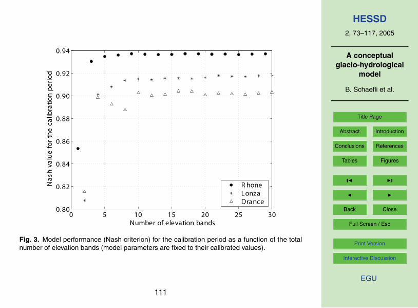
The number of elevation bands is proportionally distributed between the two types ofland cover (ice- and not ice-cover) in accordance to their percentage of the total catch-ment area. The total number determines the altitudinal resolution of the meteorological20

time series and of the corresponding simulated snow cover evolution. It has thereforea strong influence on the model performance. It can be shown through simulation, thatthere is a threshold value beyond which an increase in the number of elevation bandsdoes not result in a model performance increase (Fig. 3). For all 3 catchments, thethreshold corresponds to around 10 elevation bands (Fig. 3). The corresponding mean25

altitudinal intervals vary between 192 m (Rhone catchment) and 242 m (Drance catch-ment). Consequently, only 10 elevation bands are used for the simulations presentedin this paper.

86





HESSD2, 73–117, 2005


model

B. Schaefli et al.

Title Page



Tables Figures

J I

J I

Back Close

Full Screen / Esc

Print Version


EGU

For all simulations, the first two years are assumed to initialise the system and aretherefore discarded before the calibration criteria computation. Note that in the fol-lowing, if nothing else is stated, the numerical examples and illustrations refer to theRhone catchment.

4.1. Selection of an initial parameter set by random generation5

An initial “good” parameter set is chosen among 10 000 randomly generated parametersets. The underlying criteria are the bias between simulated and observed discharge(Eq. 14) and the classical Nash criterion (Nash and Sutcliffe, 1970).

BiasD =n∑

i=1

(Qobs,i −Qsim,i ) ·(

n∑i=1

Qobs,i

)−1

(14)

where Qobs,j is the observed discharge and Qsim,j the simulated discharge on day j .10

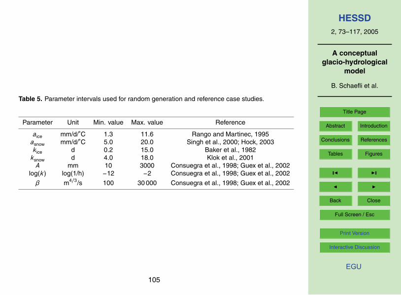
For the random generation, the parameters are supposed to be uniformly distributedwithin an interval that can be defined based on some theoretical considerations and onthe results of other case studies reported in the literature (Table 5).

Note that the value of the degree-day factor depends on the calculation procedureand especially on the time step chosen (Braithwaite and Olesen, 1989) for an numerical15

example). The above ranges must therefore be considered with care. The degree-dayfactor for ice can be assumed to be higher than for snow because of a higher albedo,meaning that the utilization of the available energy is lower for snow than for ice (Braith-waite and Olesen, 1989; Rango and Martinec, 1995). This theoretical considerationhas been confirmed by hydro-glaciological studies (Singh et al., 2000).20

The random generation within these intervals leads to Nash values higher than 0.9.For highly glacierized catchments, such high Nash values are easy to achieve as longas the model reproduces the strong seasonality of the discharge. A very simple modelcorresponding just to the mean observed discharge for each calendar day would yielda Nash value of 0.85 for the calibration period (1981–1990) and a value of 0.81 for the25

87





HESSD2, 73–117, 2005


model

B. Schaefli et al.

Title Page



Tables Figures

J I

J I

Back Close

Full Screen / Esc

Print Version


EGU

validation period (1991–1999). This means that the classical Nash criterion calculatedover the entire calibration period is not sensitive enough for further calibration.

4.2. Local refinement

Based on this first good parameter set, all the parameters are optimised by varyingone or two of them and keeping the others constant. For each parameter or couple5

of parameters an appropriate optimisation criterion is defined. The order of fine-tuningis motivated by the model sensitivity to the 7 model parameters. An initial sensitivityanalysis showed that the model performance is the most sensitive to the values of thedegree-day factors and the time constant k of the base flow component of the dis-charge. Accordingly, the degree-day factors are the first parameter couple to optimise.10

The higher the aice value is, the higher is the simulated ice melt contribution to the totalrunoff. On the other hand, ice melt only occurs when the ice surfaces are not snowcovered. The length of these time periods is directly dependent on the asnow value.The higher it is, the faster the snow cover disappears. It follows that the overall wa-ter balance - and consequently the bias between simulated and observed discharge15

and between simulated and observed annual mass balance of the glaciers - mainlydepend on these two parameters. Accordingly, the mean interannual discharge bias(BiasD, (Eq. 14) is used as an objective function for their fine-tuning. If data is avail-able, the bias between simulated and observed annual mass balance (BiasM ) is usedas a second objective function (Eq. 15).20

BiasM =1n

n∑i=1

[abs(Ba,i − B′a,i ) · abs(Ba,i )

−1] (15)

where Ba,i (m) is the observed and B′a,i (m) the estimated annual mass balance.

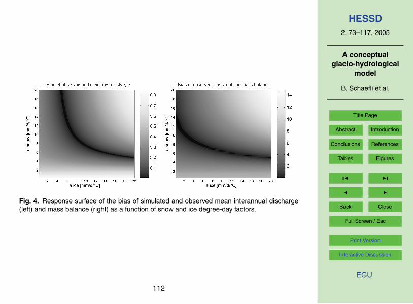
For each of these functions, a response surface is generated by varying the twodegree-day parameters. For the Rhone catchment, both surfaces show a strong corre-lation between the two parameters (Fig. 4), the local optima describing a power func-25

88





HESSD2, 73–117, 2005


model

B. Schaefli et al.

Title Page



Tables Figures

J I

J I

Back Close

Full Screen / Esc

Print Version


EGU

tion of the type asnow=α×aβice+γ where α, β and γ are constants. Hock (1999) found a

similar relationship between these two parameters. The curves described by the localoptima of both response surfaces have one intersection point. This result has an impor-tant implication: by choosing this intersection point for the calibrated values of asnow andaice, the model yields good results for the mean interannual discharge of the catchment5

and for the mass balance of the glacier. This ensures that the overall water balanceof the system is respected and that the estimated precipitation time series representswell the area-average precipitation. The estimation of this area-average precipitationin high mountainous catchments remains a very difficult task. Aellen and Funk (1990)and Kuhn (2003) pointed out that the total annual snow and ice storage change has10

about the same order of magnitude as the error committed on area-average precipita-tion estimation.

We could not find any study in the literature that uses glacier mass balance data forrigorous parameter estimation of a hydrological model for discharge simulation. Sucha cross-calibration for river discharge and glacier mass balance has been proposed15

in the past by Braun and Renner (1992) but for subjective manual calibration of thehydrological model: the mass balance data helped rejecting unrealistic parameter val-ues. Verbunt et al. (2003) used some long-term glacier mass balance aspects for aqualitative model validation.

If no glacier mass balance data is available, the choice of the parameter couple aice20

and asnow has to be based on an additional calibration criterion for simulated dailydischarge. We use the classical Nash criterion that – if computed for all local optima ofthe bias response surface – has a global optimum.

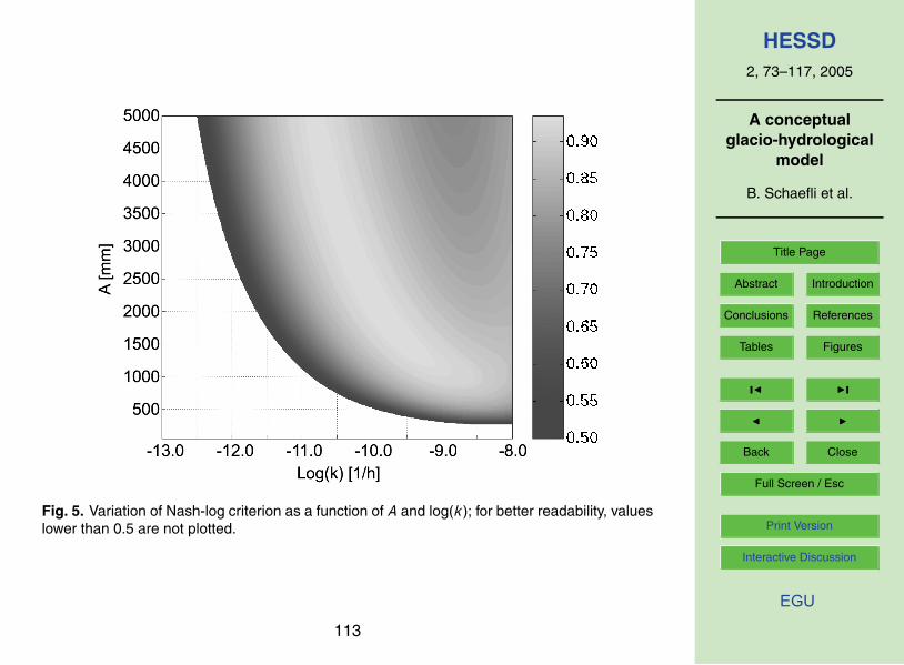
All other parameters are optimised following a similar approach. For the slow reser-voir constants A and k, the objective function corresponds to the Nash-log criterion25

89





HESSD2, 73–117, 2005


model

B. Schaefli et al.

Title Page



Tables Figures

J I

J I

Back Close

Full Screen / Esc

Print Version


EGU

(Eq. 16) as these two parameters have the most important influence on the base flow.

R2ln = 1 −

n∑i=1

[ln(Qobs,i ) − ln(Qsim,i )]2 ·

n∑i=1

[ln(Qobs,i ) −1n

n∑j=1

ln(Qobs,j )]2

−1

(16)

The response surface shows also a strong correlation between the local optima (Fig. 5).This correlation between A and k has already been highlighted in previous studies(Niggli et al., 2001; Guex et al., 2002) for catchments located at much lower elevations.5

The choice of a parameter couple is not unambiguous, for further calibration, the globaloptimum is retained. The identified relationship between the two parameters could beuseful for further sensitivity analysis.

The reservoirs coefficients ksnow and kice are optimised using the Nash criterion cal-culated for the period of snow- and ice melt (called hereafter Nash-melt criterion). This10

period has been fixed to the days between i.e. 15 July and 15 September. This ob-jective function has a global optimum. The values of these two parameters can beinterpreted as the elapsed time between the moment when melt takes place and themoment when the corresponding water volume reaches the outlet of the catchment.The ice melt water can be assumed to arrive quicker at the outlet, as the internal15

drainage systems of the glaciers are well developed when ice melt starts taking place.The snowmelt water in contrast can be stored within the snow pack leading to high timeintervals between melt and arrival at the outlet.

The remaining model parameter β influences the model quality during precipitationevents that involve direct runoff in the not ice-covered part of the catchment. These20

events are generally characterized by a sudden increase of the mean daily discharge.The chosen objective function corresponds therefore to the classical Nash criterioncalculated over all days that satisfy the following condition: the ratio between the maxi-mum discharge and the minimum discharge observed during the 3 day period includingthe preceding, the current and the following day is higher than 1.5 and the total spatial25

rainfall over the same period is higher than 10 mm. Note that the so identified days

90





HESSD2, 73–117, 2005


model

B. Schaefli et al.

Title Page



Tables Figures

J I

J I

Back Close

Full Screen / Esc

Print Version


EGU

can also include runoff events caused by other phenomena than direct runoff. Thisobjective function is called Nash peak and its response curve has a global optimum.

The elaborated parameter optimisation procedure represents a rapid and consistentcalibration tool for the glacio-hydrological model in use. Its application is subjected tothe constraint that an initial, good parameter set has been previously identified.5

5. Calibration and simulation results

5.1. Simulation of daily discharge and the hydrological regime

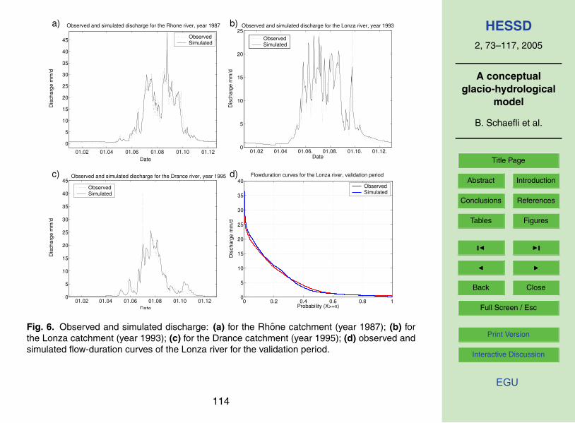
The model has been calibrated and validated for the three catchments Rhone, Lonzaand Drance. For the last two, only discharge data was available for calibration. For themodel validation, the glaciation rates of the catchments had to be updated (Table 7).10

This update is based on available topographic data. For the Drance catchment, noestimate of the glacier surface evolution was available; the used value corresponds tothe year 1995 for both periods.

The calibrated model parameters for all 3 catchments respect the theoretic consid-erations stated in Sect. 4, namely aice>asnow and kice<ksnow (Table 6). Despite its15

parsimonious structure, the model shows a good overall performance for the daily dis-charge simulation over the calibration and the validation periods (Table 7). The modelperforms particularly well for low flow situations during the winter months (Fig. 6) butalso for the periods of snowmelt in late spring and for snow- and ice melt induced highflow situations during the summer months (see the following section for further dis-20

cussion of high flow simulation). Accordingly, the model reproduces well the observedflow-duration curves (Fig. 6d).

For the Rhone and the Lonza catchment, the model performs equally well for thevalidation period as for the calibration period (Table 7). This implies in particular that theestimated mean ice-covered areas reflect sufficiently well their contribution to the total25

runoff during both periods. The Drance catchment has to be considered separately. As

91





HESSD2, 73–117, 2005


model

B. Schaefli et al.

Title Page



Tables Figures

J I

J I

Back Close

Full Screen / Esc

Print Version


EGU

mentioned before (Sect. 3), the quality of the observed discharge is considerably lowerthan for the other two other catchments, (especially during low flow situations) andthe measurement uncertainty is higher for the validation period than for the calibrationperiod, explaining partly the difference of the model performance for the two periods.

In the considered hydro-climatic region, water managers are especially interested in5

the simulation of high discharge events as they lead regularly to flood situations. Thewater management implications of these high flow situations depend on to the seasonaltiming of their appearance. Critical situations can occur during the snow- and ice meltseason when the highest annual discharges occur. These high flow events are wellsimulated by the presented discharge model (Fig. 6). At this time of the year, potential10

flood situations are generally easily managed especially through the numerous accu-mulation lakes that have been built for hydropower production all over the Swiss Alps.High discharge events occurring between mid-September and mid-October (Fig. 6b)can induce more critical situations as at this season the accumulation lakes are usuallyfilled up and cannot mitigate the floods. These situations are generally caused by im-15

portant rainfall events. In high mountainous catchments, such events can be extremelylocalized and consequently, the simulation of the corresponding discharge is stronglydependant on the representativeness of the precipitation recorded at the measurementstation (see, e.g. the high flow event in Fig. 6c, for which no rainfall was recorded). Afurther discussion of the problem of spatial representativeness of the precipitation fol-20

lows hereafter.

5.2. Simulation of glacier characteristics for the Rhone glacier

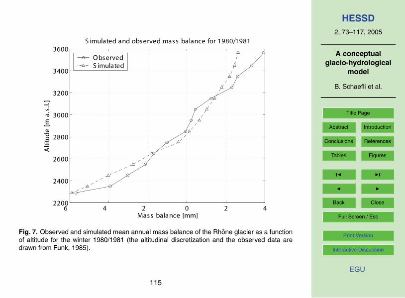
In catchments where glacier mass balance data is available, the GSM-SOCONT canbe calibrated on this data. For the Rhone catchment, the mean annual mass balanceof the Rhone glacier has been used for the calibration of the degree-day factors. Ac-25

cordingly, its total annual mass balance is well simulated (Table 8), except for the winter1981/1982, where it is considerably underestimated. The simulated value results froman ablation simulation in the lower part of the glacier up to −9 m. This unrealistic value

92





HESSD2, 73–117, 2005


model

B. Schaefli et al.

Title Page



Tables Figures

J I

J I

Back Close

Full Screen / Esc

Print Version


EGU

is due to the model assumption that the available stock of ice in a given point is infinitewhereas in reality the ice in the considered part would disappear.

The presented glacio-hydrological model reproduces also well the observed altitudi-nal distribution of the mean annual glacier mass balance (Fig. 7). This result showsthat for the studied system, the processes of snow- and ice accumulation and abla-5

tion are sufficiently well simulated through the chosen modelling approach consideringonly precipitation and temperature as underlying driving forces. In other climatic andtopographic conditions, snow redistribution by wind and avalanches could also stronglyinfluence the snow accumulation – and consequently the mass balance – at a givenpoint (see, e.g. Hartman et al., 1999; Kuhn, 2003) for an attempt to include this redistri-10

bution in a hydrological model). On the other hand, the good simulation of the altitudinaldistribution of the mean annual mass balance also indicates that the used spatial inter-polation of the meteorological time series can be assumed to be representative of thereal conditions.

Two other important descriptors are usually used to characterize a glacier: the equi-15

librium line altitude (ELA) and the accumulation area ratio (AAR). The ELA is the lineconnecting all points with zero balance at the end of a fixed year (Anonymous, 1969).It separates the ablation area from the accumulation area. The AAR is the ratio be-tween the accumulation area and the entire glacier surface. According to Ohmura etal. (1992), the equilibrium line represents the lowest boundary of the climatic glacier-20

ization, i.e. the climatic conditions which prevail at the glacier equilibrium line are con-sidered to be just sufficient to maintain the existence of ice. Ohmura et al. (1992) alsopoint out that knowledge about the ELA is essential for understanding the relation-ship between climatic changes and glacier variations. The correct simulation of theELA (respectively the AAR values) is therefore a major objective for the present hy-25

drological model that has been developed for an application in climate change impactstudies. The observed ELA and AAR values are well reproduced by the hydrologicalmodel (Table 8). For the winter 1981/1982 – even though the total annual mass bal-ance is considerably underestimated – the ELA is very well simulated. The model also

93





HESSD2, 73–117, 2005


model

B. Schaefli et al.

Title Page



Tables Figures

J I

J I

Back Close

Full Screen / Esc

Print Version


EGU

reproduces the typical linear relationship between the ELA and the total annual massbalance (Fig. 8) that is characteristic for a given glacier (Aellen and Funk, 1990; Kulka-rni, 1992; Herren et al., 2002). The simulated slope is close to the one observed in thepast.

This model feature enables its use for a glacier surface evolution model based on5

the AAR concept. This concept is classically used to reconstruct paleoclimatic glaciersurfaces (see, e.g. Porter, 1975; Torsnes et al., 1993). As shown by (Schaefli et al.,submitted manuscript) it can be used – in an extended form – for the prediction of theglacier surface for future climate conditions.

5.3. Simulation results and area-average precipitation10

As mentioned earlier in this paper, the estimation of area-average precipitation for highmountainous catchments is a considerable source of modelling uncertainty. Due to thehigh spatial variability of precipitation in such catchments, two main problems arise:i) the precipitation events recorded at the measurement station(s) are not necessarilyrepresentative for the events effectively occurred in the catchment and ii) the amount15

of precipitation at a given catchment point based on the precipitation records is difficultto estimate.

In the present modelling context, the first problem can be assumed to have an impor-tant influence on the daily discharge simulation for rainfall-induced high-flow events. Adetailed analysis would require more spatially distributed precipitation data (e.g. based20

on radar measurements) and is therefore beyond the study context. The second prob-lem is taken into account by the interpolation of the precipitation for each elevationband based on a constant altitudinal increase (cprecip) of the precipitation observedat the measurement station. In high mountainous areas, the value of cprecip is highlydifficult to estimate and it could even be justifiable to calibrate this parameter as it25

is frequently done in hydro-glaciological studies (Kuhn, 2000). Its calibration basedon discharge and glacier mass balance data would however clearly suffer from over-parameterisation, as the two degree-day factors and cprecip are mutually interdepen-

94





HESSD2, 73–117, 2005


model

B. Schaefli et al.

Title Page



Tables Figures

J I

J I

Back Close

Full Screen / Esc

Print Version


EGU

dent. The curve of optimal values of aice and asnow in terms of discharge or mass bal-ance bias undergoes a shift when varying cprecip (Fig. 9a). This shift is in the oppositedirection for the discharge bias than for the mass balance bias and consequently theintersection points between these two curves also describe a power function (Fig. 9a).If cprecip is higher than 3.6%/100 m, the value of aice of the intersection point is lower5

than the value of asnow. Such couples of degree-day factors are contrary to the basictheoretic considerations stated in Sect. 4. The smaller cprecip is, the closer are the twocurves at their right-hand tails and the less well defined is the best parameter coupleaice/asnow (Fig. 9b). For small values of cprecip the intersection point corresponds tounreasonable aice values (higher than 20 mm/d/◦C) or does not exist.10

This leads to the conclusion that it is not possible to fix a unique best value forcprecip. The multiresponse calibration through the joint use of discharge and glaciermass balance data enables however the definition of an interval of possible valuesfor cprecip that for the Rhone catchment corresponds to [2.3%/100 m, 3.8%/100 m]. Adetailed analysis of the influence of cprecip on the model ability to simulate the presented15

glaciological characteristics (AAR, ELA and altitudinal mass balance distribution) couldpossibly lead to some further conclusions.

6. Conclusions

The presented hydrological model is based on a simple reservoir approach that in-cludes the basic glacio-hydrological features, namely soil infiltration and melt water20

storage in the snow cover and the glacier. The model gives good results for meandaily discharge simulation from highly glacierized catchments as illustrated throughits application to three catchments in the Swiss Alps. It simulates well the hydrologi-cal regime and reproduces some basic glaciological features such as the total annualglacier mass balance or the accumulation area ratio. This characteristic makes the25

model particularly interesting for applications in climate change impact studies as thesimulation results can be used for glacier surface evolution studies (Schaefli et al.,

95





HESSD2, 73–117, 2005


model

B. Schaefli et al.

Title Page



Tables Figures

J I

J I

Back Close

Full Screen / Esc

Print Version


EGU

submitted manuscript). The parsimonious model structure is also adapted to such ap-plications: all required climatic input variables can be obtained from current climatemodels. Given the simplicity of the model structure and its effectiveness for dischargeand mass balance simulations, the model represents also an easy to use simulationtool to study highly glacierized alpine catchments in other contexts, such as water re-5

sources management.The elaborated procedure of parameter calibration represents a rapid and consis-

tent calibration tool for the model. The presented multisignal calibration of the riverdischarge and the glacier mass balance constitutes an interesting approach for the es-timation of the total water balance of highly glacierized catchments. In mountainous10

areas, the spatial distribution of precipitation represents an important source of uncer-tainty. Calibrated rainfall-runoff models can give good estimates of the discharge evenif the spatial precipitation is estimated poorly. Differences between simulated and realprecipitation can typically be compensated by simulated evapotranspiration or as in thepresent model by simulated ice melt. This does not represent a real problem for appli-15

cations where the main interest lies in short-term prediction of the daily discharge. Inlong-term projections however, a wrong overall water balance simulation can be signif-icantly misleading, especially in the present context where the ice melt contribution tothe runoff could be completely under- or overestimated.

The model does not account for seasonal variations of the physical system even if20

the subglacial drainage system is known to undergo a strong evolution throughout themelt season. The drainage network as well as the channel sizes vary in response tochanging water inputs (Rothlisberger, 1972; Hubbard and Nienow, 1997). This evolu-tion of the internal drainage system can be assumed to have a notable influence onthe discharge. In order to improve the discharge simulations, further investigation in25

the time-dependency of the parameters could be interesting, considering especiallypotential links between the parameters and climate variables.

It should be kept in mind that the proposed parameter calibration approach – ran-dom search completed by local refinement – guarantees neither that the globally best

96





HESSD2, 73–117, 2005


model

B. Schaefli et al.

Title Page



Tables Figures

J I

J I

Back Close

Full Screen / Esc

Print Version


EGU

parameter set nor that all possibly good parameter sets are found. A quantitative pa-rameter and model uncertainty analysis such as the one presented by Kuczera andParent 1998) would complete the current results (Schaefli et al., to be submitted2)Such an uncertainty analysis could in particular make use of the identified relation-ships between some of the model parameters and produce confidence intervals on the5

simulated daily discharge and annual glacier mass balance.

Acknowledgements. We wish to thank the Forces Motrices de Mauvoisin and the Swiss FederalOffice for Water and Geology for providing the discharge data and the national weather serviceMeteoSwiss for providing the meteorological time series. The model was developed in the con-text of the European project SWURVE (Sustainable Water: Uncertainty, Risk and Vulnerability10

in Europe, funded under the EU Environment and Sustainable Development programme, grantnumber EVK1-2000-00075) that analyses climate change impacts on water resources systemsin Europe. The Swiss part of this project was funded by the Federal Office for Education andScience, contract number 00.0117.

References15

Aellen, M. and Funk, M.: Bilan hydrologique du bassin versant de la Massa et bilan de massedes glaciers d’Aletsch (Alpes Bernoises, Suisse), In: Hydrology in Mountainous Regions I:Hydrological Measurements; the Water Cycle, edited by Lang, H. and Musy, A., IAHS Publ.No. 193, Wallingford, Oxfordshire UK, 89–98, 1990.

Anonymous: Mass-balance terms, J. Glaciol., 8, 3–7, 1969.20

Baker, D., Escher-Vetter, H., Moser, H., Oerter, H., and Reinwarth, O.: A glacier dischargemodel based on results from field studies of energy balance, water storage and flow, In:Hydrological Aspects of Alpine and High-Mountain Areas, edited by Glenn, J. W., IAHS Publ.no. 138, Wallingford, Oxfordshire UK, 103–112, 1982.

Braithwaite, R. J. and Olesen, O. B.: Calculation of glacier ablation from air temperature, West25

Greenland, In: Glacier fluctuations and climatic change, edited by Oerlemans, J., Proceed-

2Schaefli, B., Talamba, D., and Musy, A.: Quantifying hydrological modelling errors throughfinite mixture distributions, J. Hydrol., to be submitted.

97





HESSD2, 73–117, 2005


model

B. Schaefli et al.

Title Page



Tables Figures

J I

J I

Back Close

Full Screen / Esc

Print Version


EGU

ings of the Symposium on Glacier Fluctuations and Climatic Change, held in Amsterdam, 1–5 June 1987, Glaciology and quaternary geology. Kluwer Academic Publishers, Dordrecht,219–233, 1989.

Braun, L. N. and Renner, C. B.: Application of a conceptual runoff model in different physio-graphic regions of Switzerland, Hydrolog. Sci. J., 37, 217–231, 1992.5

Braun, L. N., Weber, M., and Schulz, M.: Consequences of climate change for runoff fromAlpine regions. Ann. Glaciol., 31, 19-25, 2000.

Burman, R. and Pochop, L. O.: Evaporation, evapotranspiration and climatic data, Elsevier,Amsterdam, 278, 1994.

Chen, J. and Funk, M.: Mass balance of Rhonegletscher during 1882/1983–1986/1987, J.10

Glaciol., 36, 199–209, 1990.Consuegra, D., Niggli, M., and Musy, A.: Concepts methodologiques pour le calcul des crues,

application au bassin versant superieur du Rhone, Eau, energie, air, 9/10, 223–231, 1998.Consuegra, D. and Vez, E.: AMIE – Analyse et Modelisation Integrees du cheminement des

Eaux en zones habitees, modelisation hydrologique, Application au bassin versant de la15

Haute Broye, IATE/HYDRAM, Swiss Institute of Technology, Lausanne, Lausanne, 1996.Edijatno and Michel, C.: Un modele pluie-debit journalier a trois parametres, La Houille

Blanche, 2, 113–121, 1989.Funk, M.: Raumliche Verteilung der Massenbilanz auf dem Rhonegletscher und ihre Beziehung

zu Klimaelementen, Doctoral Thesis, Eidgenossische Technische Hochschule Zurich,20

Zurich, 183, 1985.Guex, D., Guex, F., Pugin, S., Hingray, B., and Musy, A.: Regionalisation of hydrological pro-

cesses in view of improving model transposability. WP3 Final Report of the Pan-EuropeanFRHYMAP Project (Flood Risk scenarios and Hydrological MAPping), No. Contract CE:3/NL/1/164/99 15 183 01., Swiss Institute of Technology, Lausanne, Lausanne, 2002.25

Haeberli, W., Frauenfelder, R., and Hoelzle, M. (eds.): Glacier mass balance bulletin no. 7(2000–2001). IAHS – UNEP – UNESCO – WMO, Zurich, Switzerland, 87, 2003.

Hartman, M. D., Baron, J. S., Lammers, R. B., Cline, D. W., Band, L. E., Liston, G. E., andTague, C.: Simulations of snow distribution and hydrology in a mountain basin, Water Resour.Res., 35, 1587–1603, 1999.30

Herren, E. R., Bauder, A., Hoelzle, M. and Maisch, M.: The Swiss Glaciers 1999/2000 and2001/2002. 121/122, Glaciological Commission (GC) of the Swiss Academy of Sciences(SAS), Zurich, 2002.

98





HESSD2, 73–117, 2005


model

B. Schaefli et al.

Title Page



Tables Figures

J I

J I

Back Close

Full Screen / Esc

Print Version


EGU

Herren, E. R., Hoelzle, M., and Maisch, M.: The Swiss Glaciers 1997/1998 and 1998/1999.119/120, Glaciological Commission (GC) of the Swiss Academy of Sciences (SAS), Zurich,2001.

Hock, R.: A distributed temperature-index ice- and snowmelt model including potential directsolar radiation, J. Glaciol., 45, 101–111, 1999.5

Hock, R.: Temperature index melt modelling in mountain areas, J. Hydrol., 282, 104–115, 2003.Hubbard, B. and Nienow, P.: Alpine subglacial hydrology, Quat. Sci. Rev., 16, 939–955, 1997.Klok, E. J., Jasper, K., Roelofsma, K. P., Gurtz, J., and Badoux, A.: Distributed hydrological

modelling of a heavily glaciated Alpine river basin, Hydrolog. Sci. J., 46, 553—570, 2001.Kuczera, G. and Parent, E.: Monte Carlo assessment of parameter uncertainty in conceptual10

catchment models: the Metropolis algorithm, J. Hydrol., 211, 69–85, 1998.Kuhn, M.: Verification of a hydrometeorological model fo glacierized basins, Ann. Glaciol., 31,

15—18, 2000.Kuhn, M.: Redistribution of snow and glacier mass balance from a hydrometeorological model,

J. Hydrol., 282, 95–103, 2003.15

Kulkarni, A. V.: Mass balance of Himalayan glaciers using AAR and ELA methods, J. Glaciol.,38, 101–104, 1992.

Kustas, W. P. and Rango, A.: A simple energy budget algorithm for the snowmelt runoff model,Water Resour. Res., 30, 1515–1527, 1994.

Nash, J. E. and Sutcliffe, J. V.: River flow forecasting through conceptual models, Part I, a20

discussion of principles, J. Hydrol., 10, 282–290, 1970.Niggli, M., Hingray, B., and Musy, A.: A Methodology for Producing Runoff Maps and Assessing

the Influence of Climat Change in Europe in WRINCLE (Water Resources: Influence ofClimate Change in Europe), Swiss Federal Institute of Technology Lausanne, Lausanne,2001.25

Ohmura, A.: Physical basis for the temperature-based melt-index method, J. Appl. Meteorol.,40, 753–761, 2001.

Ohmura, A., Kasser, P., and Funk, M.: Climate at the equilibrium line of glaciers, J. Glaciol., 38,397–411, 1992.

Paterson, W. S. B.: The Physics of Glaciers, Pergamon, Oxford, 480, 1994.30

Porter, S. C.: Equilibrium-line altitudes of late quaternary glaciers in southern alps, NewZealand, Quaternary Research, 5, 27–47, 1975.

Rango, A. and Martinec, J.: Revisiting the degree-day method for snowmelt computations,

99





HESSD2, 73–117, 2005


model

B. Schaefli et al.

Title Page



Tables Figures

J I

J I

Back Close

Full Screen / Esc

Print Version


EGU

Water Resour. Bull., 31, 657–669, 1995.Rothlisberger, H.: Water pressure in intra- and subglacial channels, J. Glaciol., 11, 177–203,

1972.Singh, P. and Kumar, N.: Impact assessment of climate change on the hydrological response of

a snow and glacier melt runoff dominated Himalayan river, J. Hydrol., 193, 316–350, 1997.5

Singh, P., Kumar, N., and Arora, M.: Degree-day factors for snow and ice for Dakriani Glacier,Garhwal Himalayas, J. Hydrol., 235, 1–11, 2000.

Spreafico, M., Weingartner, R., and Leibundgut, C.: Atlas hydrologique de la Suisse, ServiceHydrologique et Geologique National (SHGN), Bern, 1992.

SwissTopo: Digital height model of Switzerland – DHM25, Waber, Switzerland, 1995.10

SwissTopo: Digital National Maps of Switzerland – PM25, Waber, Switzerland, 1997.Torsnes, I., Rye, N., and Nesje, A.: Modern and little ice-age equilibrium-line altitudes on outlet

valley glaciers from Jostedalsbreen, Western Norway – an evaluation of different approachesto their calculation, Arctic and Alpine Research, 25, 106–116, 1993.

Verbunt, M., Gurtz, J., Jasper, K., Lang, H., Warmerdam, P., and Zappa, M.: The hydrological15

role of snow and glaciers in alpine river basins and their distributed modeling, J. Hydrol., 282,36–55, 2003.

Willis, I. and Bonvin, J.-M.: Climate change in mountain environments: hydrological and waterresource implications, Geography, 80, 247–261, 1995.

WMO: Intercomparison of models of snowmelt runoff, WMO, Geneva, 1986.20

100





HESSD2, 73–117, 2005


model

B. Schaefli et al.

Title Page



Tables Figures

J I

J I

Back Close

Full Screen / Esc

Print Version


EGU

Table 1. Main physiographic characteristics of the three catchments (reference year for glacia-tion: 1985) and the estimated precipitation increase with altitude (cprecip).

River Area Glaciation Mean altitude Altitude range Mean slope cprecip

(km2) (%) (m a.s.l.) (m a.s.l.) (◦) (%/100 m)

Rhone 38.9 52.2 2713 1755–3612 22.9 3.1Lonza 77.8 36.5 2601 1520–3890 30.0 7.9Drance 169.3 41.4 2940 1961–4305 26.7 2.2

101





HESSD2, 73–117, 2005


model

B. Schaefli et al.

Title Page



Tables Figures

J I

J I

Back Close

Full Screen / Esc

Print Version


EGU

Table 2. Meteorological conditions of the three catchments (reference altitude 2800 m a.s.l.,reference period 1974–1994).

River Estimated mean Estimated dailyannual precipitation (mm/yr) mean temperature (◦C)

Rhone 2005 −5.9Lonza 2304 −3.9Drance 1449 −3.2

102





HESSD2, 73–117, 2005


model

B. Schaefli et al.

Title Page



Tables Figures

J I

J I

Back Close

Full Screen / Esc

Print Version


EGU

Table 3. Meteorological measurement stations used for precipitation (P ) and temperature (T )time series and their spatial situation compared to the studied catchments.

River Station name Measured Station altitude Distance to Distance tovariable (m a.s.l.) catchment nearest, farthest

centroid (km) catchment point (km)

Rhone Oberwald P 1375 8.1 [3.0, 14.2]Rhone Ulrichen T 1345 12.3 [7.4, 18.4]Lonza Ried P , T 1480 6.8 [ 1.0, 13.7]Drance Mauvoisin P , T 1841 5.1 [ 0.7, 12.7]

103





HESSD2, 73–117, 2005


model

B. Schaefli et al.

Title Page



Tables Figures

J I

J I

Back Close

Full Screen / Esc

Print Version


EGU

Table 4. Time periods used for the model calibration and validation for the three catchments.

River Discharge Mass balance Dischargevalidation calibration calibration

Rhone 1981–1990 1991–1999 1979–1982Lonza 1974–1984 1985–1994 –Drance 1995–1999 1990–1994 –

104





HESSD2, 73–117, 2005


model

B. Schaefli et al.

Title Page



Tables Figures

J I

J I

Back Close

Full Screen / Esc

Print Version


EGU

Table 5. Parameter intervals used for random generation and reference case studies.

Parameter Unit Min. value Max. value Reference

aice mm/d/◦C 1.3 11.6 Rango and Martinec, 1995asnow mm/d/◦C 5.0 20.0 Singh et al., 2000; Hock, 2003kice d 0.2 15.0 Baker et al., 1982ksnow d 4.0 18.0 Klok et al., 2001A mm 10 3000 Consuegra et al., 1998; Guex et al., 2002

log(k) log(1/h) −12 −2 Consuegra et al., 1998; Guex et al., 2002

β m4/3/s 100 30 000 Consuegra et al., 1998; Guex et al., 2002

105





HESSD2, 73–117, 2005


model

B. Schaefli et al.

Title Page



Tables Figures

J I

J I

Back Close

Full Screen / Esc

Print Version


EGU

Table 6. Calibrated parameter values for the 3 catchments and the used glaciation rates.

Parameter Unit Rhone Lonza Drance

aice mm/d/◦C 11.5 7.1 8.0asnow mm/d/◦C 6.6 6.1 4.5A mm 2147 710 1464

log(k) log(1/h) −9.9 −7.4 −10.8kice d 4.7 1.7 4.6ksnow d 5.2 4.0 5.9

β m4/3/s 301 2342 1213

106





HESSD2, 73–117, 2005


model

B. Schaefli et al.

Title Page



Tables Figures

J I

J I

Back Close

Full Screen / Esc

Print Version


EGU

Table 7. Calibration criteria values (Nash, Nash-log and bias) for the 3 catchments for thecalibration and the validation period; for both periods, the used glaciation rates are indicated.

Criterion Period Rhone Lonza Drance

Nash Calibration 0.94 0.92 0.90Nash Validation 0.92 0.91 0.84

Nash-log Calibration 0.93 0.88 0.83Nash-log Validation 0.93 0.93 0.79

Bias Calibration −0.03 −0.02 0.00Bias Validation −0.00 0.03 0.05

Glaciation Calibration 0.52 0.38 0.41Glaciation Validation 0.50 0.36 0.41

107





HESSD2, 73–117, 2005


model

B. Schaefli et al.

Title Page



Tables Figures

J I

J I

Back Close

Full Screen / Esc

Print Version


EGU

Table 8. Simulated and observed total annual mass balance, AAR and ELA.

Mass balance (mm/yr) AAR (%) ELA (m a.s.l.)Year Observed Simulated Obs. Sim. Obs. Sim.

1979/1980 890 835 64 75 2764 26821980/1981 90 115 53 60 2875 28311981/1982 −380 −1110 45 36 3035 3023

108





HESSD2, 73–117, 2005


model

B. Schaefli et al.

Title Page



Tables Figures

J I

J I

Back Close

Full Screen / Esc

Print Version


EGU

Altitudinal interpolation

Temperature Precipitation

Rain

Rainfall - / snow fall separation

Snow

Unit icecovered?

Yes No

Computation of snow-and ice pack evolution

Meltwater - runoff transformation

Runoff

Computation of snowpack

Melt


Runoff

Snow heightMeltSnow height

Potential ET

Actual ET

Altitudinal interpolation

Temperature Precipitation

Rain

Rainfall - / snow fall separation

Snow

Unit icecovered?

Yes No

Computation of snow-and ice pack evolution


Runoff

Computation of snowpack

Melt


Runoff

Snow heightMeltSnow height

Potential ET

Actual ET

Fig. 1. Hydrological model structure for one spatial unit.

109





HESSD2, 73–117, 2005


model

B. Schaefli et al.

Title Page



Tables Figures

J I

J I

Back Close

Full Screen / Esc

Print Version


EGU

Fig. 2. Location of the case study catchments in the Swiss Alps (SwissTopo, 1997).

110





HESSD2, 73–117, 2005


model

B. Schaefli et al.

Title Page



Tables Figures

J I

J I

Back Close

Full Screen / Esc

Print Version


EGU

0 5 10 15 20 25 300.80

0.82

0.84

0.86

0.88

0.90

0.92

0.94

Number of elevation bands

Na

sh v

alu

e f

or

the

ca

libra

tion

pe

rio

d

R honeLonzaDrance

Fig. 3. Model performance (Nash criterion) for the calibration period as a function of the totalnumber of elevation bands (model parameters are fixed to their calibrated values).

111





HESSD2, 73–117, 2005


model

B. Schaefli et al.

Title Page



Tables Figures

J I

J I

Back Close

Full Screen / Esc

Print Version


EGU

Fig. 4. Response surface of the bias of simulated and observed mean interannual discharge(left) and mass balance (right) as a function of snow and ice degree-day factors.

112





HESSD2, 73–117, 2005


model

B. Schaefli et al.

Title Page



Tables Figures

J I

J I

Back Close

Full Screen / Esc

Print Version


EGU

0.90

0.85

0.80

0.75

0.70

0.65

0.60

0.55

0.50

Fig. 5. Variation of Nash-log criterion as a function of A and log(k); for better readability, valueslower than 0.5 are not plotted.

113





HESSD2, 73–117, 2005


model

B. Schaefli et al.

Title Page



Tables Figures

J I

J I

Back Close

Full Screen / Esc

Print Version


EGU

01.02 01.04 01.06 01.08 01.10 01.12

0

5

10

15

20

25

30

35

40

45

Date

Dis

charg

e m

m/d

Observed and simulated discharge for the Rhone river, year 1987

ObservedSimulated

01.02 01.04 01.06. 01.08. 01.10. 01.12.0

5

10

15

20

25Observed and simulated discharge for the Lonza river, year 1993

Dis

charg

e m

m/d

Date

ObservedSimulated

01.02 01.04 01.06 01.08 01.10 01.120

5

10

15

20

25

30

35

40

45

Date

Dis

charg

e m

m/d

ObservedSimulated

Observed and simulated discharge for the Drance river, year 1995

0 0.2 0.4 0.6 0.8 10

5

10

15

20

25

30

35

40Flowduration curves for the Lonza river, validation period

Dis

charg

e m

m/d

Probability (X>=x)

ObservedSimulated

a)

c)

b)

d)

Fig. 6. Observed and simulated discharge: (a) for the Rhone catchment (year 1987); (b) forthe Lonza catchment (year 1993); (c) for the Drance catchment (year 1995); (d) observed andsimulated flow-duration curves of the Lonza river for the validation period.

114





HESSD2, 73–117, 2005


model

B. Schaefli et al.

Title Page



Tables Figures

J I

J I

Back Close

Full Screen / Esc

Print Version


EGU

6 4 2 0 2 42200

2400

2600

2800

3000

3200

3400

3600S imulated and observed mass balance for 1980/1981

Mass balance [mm]

Alti

tud

e [

m a

.s.l.

]

ObservedS imulated

Fig. 7. Observed and simulated mean annual mass balance of the Rhone glacier as a functionof altitude for the winter 1980/1981 (the altitudinal discretization and the observed data aredrawn from Funk, 1985).

115





HESSD2, 73–117, 2005


model

B. Schaefli et al.

Title Page



Tables Figures

J I

J I

Back Close

Full Screen / Esc

Print Version


EGU

3000 2500 2000 1500 1000 500 0 500 10002600

2700

2800

2900

3000

3100

3200S imulated and observed E LA and mass balance

Mass balance [mm]

EL

A [

m a

.s.l.

]

Observed 1884/85-1907/08 & 1979/80-1981/82S imulated 1979/80-1998/99

Fig. 8. ELA versus annual mass balance: observed values for 1884/1885–1907/1908and 1979/1980–1981/1982 (Chen and Funk, 1990) and simulated values for 1979/1980–1998/1999.

116





HESSD2, 73–117, 2005


model

B. Schaefli et al.

Title Page



Tables Figures

J I

J I

Back Close

Full Screen / Esc

Print Version


EGU

0 5 10 15 200

2

4

6

8

10

12

14

16

18

20

a s

no

w [

mm

/d/°

C]

a ice [mm/d/°C ]

Optimal agl/an as a function of altitudinal interpolation of precipitation

B ’ Q (cprecip 2.5)

0 5 10 15 200

2

4

6

8

10

12

14

16

18

20

a s

no

w [

mm

/d/°

C]

a ice [mm/d/°C ]

Optimal agl/an as a function of altitudinal interpolation of precipitation






B ’ Q (cprecip 3.7)Intersections

a) b)

Fig. 9. Optimal curves of mass balance and discharge bias as a function of aice, asnow andcprecip; values of cprecip in brackets (unit: %/100 m).

117





A Conceptual Glacio-hydrological Model

Documents

Transcript of A Conceptual Glacio-hydrological Model